Download Installation Manual X3M-D Flash D

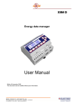
Flash D
Electrec Energy Analyzer
User Manual
Version 8 November 2005
The document can be modified without prior information.
Pag. 1 di 84
Index
INTRODUCTION ............................................................................................................................5
1.1 COPYRIGHT ......................................................................................................................5
1.2 WARRANTY .......................................................................................................................5
1.3 RETURN AND REPAIR FORMALITIES ..............................................................................5
1.3.1 RE-SHIPPING OF REPAIRED PRODUCT ..................................................................5
1.3.2 Return Material Authorization (RMA form) .................................................................6
2 Safety ......................................................................................................................................7
2.1 Operator safety..................................................................................................................7
3 Mounting .................................................................................................................................8
3.1 Instruments size (mm).......................................................................................................8
3.2 Optional modules size (mm)..............................................................................................8
3.3 Fixing and blocking............................................................................................................8
4 Wiring diagrams ......................................................................................................................9
4.1 Power supply.....................................................................................................................9
4.2 Measurement connections ................................................................................................9
4.2.1 Voltage connection .....................................................................................................9
4.2.2 Current connection .....................................................................................................9
4.2.3 4W Star connection (4 wire) .....................................................................................10
4.2.4 3W Delta connection (3 wire)....................................................................................11
4.2.4.1
Connection with 2 CTs on L1 and L3...............................................................11
4.2.4.2
Connection with 2 CTs on L1 and L2...............................................................12
4.2.5 2 Wire connection (single phase) .............................................................................12
4.2.6 2 Wire connection (bi-phase)....................................................................................13
4.3 Outputs connection .........................................................................................................13
4.4 Optional modules connection ..........................................................................................14
4.4.1 RS485 Option ...........................................................................................................14
4.4.2 RS232 Option ...........................................................................................................15
4.4.3 Dual 4-20 mA analog output option ..........................................................................15
5 Instrument use ......................................................................................................................16
5.1 Instrument set up.............................................................................................................16
5.1.1 Set up sequence.......................................................................................................17
5.1.2 Configuration procedure ...........................................................................................18
5.1.2.1
Electrical system configuration ........................................................................18
5.1.2.2
Communication characteristics configuration ..................................................20
5.1.2.3
Digital Outputs configuration ...........................................................................20
5.1.2.4
Pulse characteristics configuration ..................................................................21
5.1.2.4.1
5.1.2.5
5.1.2.5.1
5.1.2.6
5.1.2.6.1
5.1.2.6.2
Pulse output set up with Modbus registers.................................................................. 21
Alarm configuration..........................................................................................22
Alarm set up with Modbus registers. ........................................................................... 23
4-20 mA Analog Outputs configuration............................................................24
Analog output set up with Modbus registers. .............................................................. 25
Alarms and 4-20 mA output configuration for the average (AVG) parameters ........... 25
5.1.2.7
Contrast adjustment.........................................................................................25
5.1.3 Reset Procedure.......................................................................................................26
5.1.3.1
Average and Max Demand power Reset.........................................................26
5.1.3.2
Energy Reset ...................................................................................................26
5.2 Readings .........................................................................................................................27
5.2.1 Readings selection keys ...........................................................................................27
Pag. 2 di 84
5.2.1.1
5.2.1.1.1
5.2.1.1.2
5.2.1.1.3
5.2.1.1.4
5.2.1.1.5
5.2.1.1.6
5.2.1.2
5.2.1.2.1
5.2.1.2.2
5.2.1.2.3
5.2.1.2.4
5.2.1.2.5
5.2.1.3
5.2.1.3.1
5.2.1.3.2
5.2.1.3.3
5.2.1.3.4
5.2.1.3.5
5.2.1.4
5.2.1.4.1
5.2.1.4.2
5.2.1.4.3
5.2.1.4.4
Voltage and Frequency readings.....................................................................27
3P 4 W Configuration .................................................................................................. 27
3P 3 W Configuration .................................................................................................. 28
3P-b 4W Configuration ................................................................................................ 28
3P-b 3W Configuration ................................................................................................ 28
1P 2W Configuration ................................................................................................... 28
2P 2W Configuration ................................................................................................... 28
Current readings ..............................................................................................29
3P 4W Configuration ................................................................................................... 29
3P 3W Configuration ................................................................................................... 29
3P-b 4W Configuration ................................................................................................ 29
3P-b 3W Configuration ................................................................................................ 29
1P 2W and 2P 2W Configuration ................................................................................ 29
Powers.............................................................................................................30
3P 4W Configuration ................................................................................................... 30
3P 4W only Import Configuration................................................................................. 30
3P 3W / 3P-b 3W / 2P 2W Configuration .................................................................... 31
3P-b 4W Configuration ................................................................................................ 32
1P 2W Configuration ................................................................................................... 32
P.F. Visualization .............................................................................................33
3P 4W Configuration ................................................................................................... 33
3Pb 4W Configuration ................................................................................................. 33
3P 3W e 3Pb 3W Configuration................................................................................... 33
1P 2W e 2P 2W Configuration..................................................................................... 33
5.2.1.5
Life Time ..........................................................................................................33
5.2.1.6
Energies ..........................................................................................................34
5.2.1.7
Only Import Energy Display .............................................................................34
6 Instrument Description ..........................................................................................................35
6.1 Introduction......................................................................................................................35
6.2 Simplicity and versatility ..................................................................................................35
6.3 Total harmonic distortion Measurement (THD) ...............................................................36
6.4 Energy Measurement ......................................................................................................36
6.5 Calibration Led ................................................................................................................36
6.6 Digital Outputs.................................................................................................................36
6.7 Oulse Output ...................................................................................................................36
6.8 Alarms .............................................................................................................................36
6.9 Communication ...............................................................................................................37
6.10
Average and peak Energy............................................................................................37
7 System Architecture ..............................................................................................................37
7.1 General Features ............................................................................................................37
7.1.1 FLASH D...................................................................................................................37
7.1.2 Options .....................................................................................................................38
7.1.2.1
RS485 Port ......................................................................................................38
7.1.2.2
RS232 Port ......................................................................................................38
7.1.2.3
2 x 4-20 mA Analog Output .............................................................................38
8 Parameters and formulas ......................................................................................................39
8.1 3P 4W Three phase with 4 wire neutral .........................................................................39
8.1.1 Available Reading:....................................................................................................39
8.1.2 Measurement Formulas:...........................................................................................42
8.2 3P 3W Three phase without neutral ................................................................................44
8.2.1 Available Reading:....................................................................................................44
8.2.2 Measurement Formulas:...........................................................................................46
Pag. 3 di 84
8.3 3P-b 4W Balanced Three phase with neutral.................................................................48
8.3.1 Available Reading:....................................................................................................48
8.3.2 Measurements Formulas: .........................................................................................50
8.4 3P-b 3W Balanced three Phase without neutral 3 wires ...............................................51
8.4.1 Available Reading:....................................................................................................51
8.4.2 Measurement Formulas:...........................................................................................53
8.5 1P (2W) Single phase ....................................................................................................54
8.5.1 Available Reading:....................................................................................................54
8.5.2 Measurement Formulas:...........................................................................................56
8.6 2P (2W) Double phase ...................................................................................................57
8.6.1 Available Reading:....................................................................................................57
8.6.2 Measurements Formulas: .........................................................................................59
8.6.3 Sampling:..................................................................................................................60
8.6.4 Grid frequency Measurement: ..................................................................................60
8.7 Average values and energy Calculation..........................................................................60
8.7.1 Energy counting........................................................................................................60
8.7.2 Average Powers / maximum demand (m/Max).........................................................60
8.7.3 HOLD function ..........................................................................................................61
8.7.4 Synchronization ........................................................................................................61
9 MODBUS Protocol ...............................................................................................................62
9.1 Foreword: ........................................................................................................................62
9.2 “Device dependent” Functions ........................................................................................63
9.2.1 (0x11) Slave ID Report .............................................................................................63
9.2.2 (0x07) Exception Status Read ..................................................................................64
9.3 “User defined” Functions .................................................................................................64
9.3.1 (0x42) Slave Address Change..................................................................................64
9.4 Register Mapping ............................................................................................................65
9.4.1 Holding registers.......................................................................................................65
9.4.2 Parameter selection tables .......................................................................................69
9.4.3 Flas-D Input registers ...............................................................................................73
9.4.4 Input Registers (backward compatibility area) ..........................................................77
9.4.5 Coils (back compatibility) ..........................................................................................80
9.4.6 FLASH D coils ..........................................................................................................80
10
Technical Characteristics ..................................................................................................81
11
Firmware Revisions ...........................................................................................................83
12
Order codes .......................................................................................................................83
13
DECLARATION OF CONFORMITY ..................................................................................83
Pag. 4 di 84
INTRODUCTION
We thank you for choosing an Electrex instrument
We invite you to carefully read this instructions manual for the best use of the Flash D instruments.
1.1 COPYRIGHT
Electrex S.r.l. All rights are reserved.
It is forbidden to duplicate, adapt, transcript this document without Electrex written authorization, except
when regulated accordingly by the Copyright Laws.
Copyright© 2003-2004
1.2 WARRANTY
This product is covered by a warranty against material and manufacturing defects for a period of 36
months period from the manufacturing date
The warranty does not cover the defects that are due to:
• Negligent and improper use
• Failures caused by atmospheric hazards
• Acts of vandalism
• Wear out of materials
Electrex reserves the right, at its discretion, to repair or substitute the faulty products
The warranty is not applicable to the products that will result defective in consequence of a negligent and
improper use or an operating procedure not contemplated in this manual.
1.3 RETURN AND REPAIR FORMALITIES
Electrex accepts the return of instruments for repair only when authorized in advance. For instrument
purchased directly, the repair authorization must be requested to Electrex directly by using the enclosed
RMA form. We recommend otherwise to contact your local distributor for assistance on the return/repair
formalities. In both the cases, the following information must be supplied:
•
Company full data
•
Contact name for further communication
•
Product description
•
Serial number
•
Description of the returned accessories
•
Invoice / Shipping document number and date
•
Detailed description of the fault and of the operating condition when the fault occurred
The Electrex repair lab will send the authorization number to the customer directly or to the distributor as
per applicable case. The RMA authorization number shall be clearly marked on the packaging and on the
return transport document.
WARNING: Failure to indicate the RMA number on the external packaging will entitle our warehouse to
refuse the delivery upon arrival and to return the parcel at sender’s charge.
The material must be shipped:
- within 15 working days from the receipt of the return authorization number
- free destination i.e. all transport expenses at sender’s charge.
- to the following address:
Electrex S.r.l.
Via Claudia 96 - 41056 Savignano s/P (MO) - Italy
Atn. Repair laboratory
- the units covered by warranty must be returned in their original packaging.
1.3.1 RE-SHIPPING OF REPAIRED PRODUCT
The terms for re-shipment of repaired products are ex-works, i.e. the transport costs are at customer
charge.
Products returned as detective but found to be perfectly working by our laboratories, will be charged a
fixed fee (40.00 Euro + VAT where applicable) to account for checking and testing time irrespective of the
warranty terms.
Pag. 5 di 84
1.3.2 Return Material Authorization (RMA form)
Request for the authorization number for the return of goods
Date:
Company:
Contact name:
TEL:
FAX:
Product description:
Serial number:
Description of the returned accessories (if any):
Original purchase Invoice (or Shipping document) number and date.
NB: The proof of purchase must be provided by the customer. Failure to complete this area will automatically void all warranty.
Detailed description of the malfunction and of the operating conditions when the fault occurred
Tick off for a quotation
Should a product be found by our laboratories to be perfectly working, a fixed amount of 40 Euro (+VAT if applicable) will be charged
to account for checking and testing time irrespective of the warranty tems.
Space reserved to ELECTREX
R.M.A. No.
The RMA number shall be clearly indicated on the external packaging and on the shipping document:. Failure to observe this
requirement will entitle the ELECTREX warehouse to refuse the delivery.
Pag. 6 di 84
2 Safety
This instrument was manufactured and tested in compliance with IEC 61010 class 2 standards for
operating voltages up to 250 VAC rms phase to neutral.
In order to maintain this condition and to ensure safe operation, the user must comply with the indications
and markings contained in the following instructions:
• When the instrument is received, before starting its installation, check that it is intact and no
damage occurred during transport.
• Before mounting, ensure that the instrument operating voltages and the mains voltage are
compatible then proceed with the installation.
• The instrument power supply needs no earth connection.
• The instrument is not equipped with a power supply fuse; a suitable external protection fuse must
be foreseen by the contractor.
• Maintenance and/or repair must be carried out only by qualified, authorized personnel
• If there is ever the suspicion that safe operation is no longer possible, the instrument must be
taken out of service and precautions taken against its accidental use.
• Operation is no longer safe when:
1) There is clearly visible damage.
2) The instrument no longer functions.
3) After lengthy storage in unfavorable conditions.
4) After serious damage occurred during transport
The instruments FLASH D must be installed in respect of all the local regulations.
2.1
Operator safety
Warning:
-
-
-
Precautions:
-
Failure to observe the following instructions may lead to a serious danger of death.
During normal operation dangerous voltages can occur on instrument terminals and on
voltage and current transformers. Energized voltage and current transformers may
generate lethal voltages. Follow carefully the standard safety precautions while carrying
out any installation or service operation.
The terminals of the instrument must not be accessible by the user after the installation.
The user should only be allowed to access the instrument front panel where the display is
located.
Do not use the digital outputs for protection functions nor for power limitation functions.
The instrument is suitable only for secondary protection functions.
The instrument must be protected by a breaking device capable of interrupting both the
power supply and the measurement terminals. It must be easily reachable by the operator
and well identified as instrument cut-off device.
The instrument and its connections must be carefully protected against short-circuit.
Failure to respect the following instructions may irreversibly damage to the instrument.
The instrument is equipped with PTC current limiting device but a suitable external
protection fuse should be foreseen by the contractor.
The outputs and the options operate at low voltage level; they cannot be powered by any
unspecified external voltage.
The application of currents not compatible with the current inputs levels will damage to the
instrument.
Pag. 7 di 84
3 Mounting
3.1
Instruments size (mm)
6 DIN rail modules
3.2
Optional modules size (mm)
2 DIN rail modules.
3.3
Fixing and blocking
The instrument (as well as the optional modules) are fixed to the DIN rail by means of the spring clip
located on the rear side of the unit.
Pag. 8 di 84
4 Wiring diagrams
4.1
Power supply
The instrument is fitted with a separate power supply with extended
operating range. The power supply terminals are numbered (10) and (11).
Use cables with max cross-section of 4 mm2.
4.2
Measurement connections
4.2.1 Voltage connection
Use cables with max cross-section of 4 mm2 and connect them to the terminals marked VOLTAGE INPUT
on the instrument according to the applicable diagrams that follow.
4.2.2 Current connection
It is necessary to use external CTs with a primary rating adequate to the load to be metered and with a 5A
secondary rating. The number of CTs to be used (1, 2 or 3) depends upon the type of network.
Connect the CT output(s) to the terminals marked CURRENT INPUT of the instrument according to the
applicable diagrams that follow.
Use cables with cross-section adequate to the VA rating of the CT and to the distance to be covered. The
max cross-section for the terminals is 4 mm2.
N.B. The CT secondary must always be in short circuit when not connected to the instrument in order to
avoid damages and risks for the operator.
Warning: THE PHASE RELATIONSHIP AMONG VOLTAGE AND CURRENT SIGNALS MUST BE
CAREFULLY RESPECTED. ALL DISREGARD OF THIS RULE OR OF THE WIRING
DIAGRAM LEADS TO SEVERE MEASUREMENT ERRORS.
Pag. 9 di 84
4.2.3 4W Star connection (4 wire)
Low voltage
3 CTs
Configuration 3Ph/4W
High voltage
3 PTs 3 CTs
Configuration 3Ph/4W
Low Voltage
1 CT (symmetrical and balanced load)
Configuration 3Ph/4W-Bal
Pag. 10 di 84
4.2.4 3W Delta connection (3 wire)
Connection with 3 CTs
Connection with 1 CT
Low Voltage
3 CTs (unbalanced load)
Configuration 3Ph/3W
Low Voltage 1 CT (symmetrical and balanced load)
Configuration 3Ph/3W-Bal
4.2.4.1
Connection with 2 CTs on L1 and L3
Low Voltage
2 CTs
Configuration 3Ph/3W
High Voltage 2 PTs 2 CTs
Configuration 3Ph/3W
Pag. 11 di 84
4.2.4.2 Connection with 2 CTs on L1 and L2
Low Voltage
2 CTs
Configuration 3Ph/3W
High Voltage 2 PTs 2 CTs
Configuration 3Ph/3W
4.2.5 2 Wire connection (single phase)
Low Voltage (phase-neutral)
Configuration
1 CT
1Ph/2W
Pag. 12 di 84
4.2.6 2 Wire connection (bi-phase)
Low Voltage (phase-phase)
Configuration
4.3
1 CT
2Ph/2W
Outputs connection
The instrument is equipped with two opto-isolated transistor outputs rated 27 Vdc, 27 mA (DIN 43864
standards).
The outputs working mode is set by default to operate as pulse output proportional to the Active energy
(output 1) and to the Reactive energy (output 2). They support an output rate of 1.000 pulses per kWh (or
kvarh) referred to the instrument input range without any CT and PT multiplier.
In order to calculate the energy value of each pulse the following formula must be considered.
KP =
KCT × K PT
Pulse / kWh
Where: Kp = energy of each pulse; KCT = CT ratio ; KPT = PT ratio ;
Pulse/kWh = Pulse rate
Example: CT = 100/5; PT = 20.000/100 K P =
20 × 200
= 4kWh / pulse or kWh = Pulse count/4
1000
Other pulse rate settings may be however programmed as described in the instrument set up section.
The operating mode of the digital outputs may also be changed to work as alarm output or as remote
output device controlled by the Modbus protocol as described in the instrument set up section.
Pag. 13 di 84
4.4
Optional modules connection
The optional modules shall be placed beside of the instrument and shall be connected to the same by
means of the cable supplied with.
The optional modules are self-supplied; the instrument recognises the type of option(s) connected and the
applicable programming menu will automatically appear when necessary.
CN1 connector: suitable for the RS485 or RS232 optional modules
CN2 connector: suitable for the 4-20 mA optional module or for the Hardware up-date key
4.4.1 RS485 Option
RS485 pin out
1
2
3
Pag. 14 di 84
A +
B Shield
4.4.2 RS232 Option
RS232 pin out
1
2
3
4
5
6
DSR (Handshake to DTE)
CTS (Handshake to DTE)
RD (Data to DTE)
TD (Data from DTE)
RTS (Handshake from DTE)
GND
4.4.3 Dual 4-20 mA analog output option
4-20 mA pin out
1
2
3
CH1 Channel 1
CH2 Channel 2
Source Common +
NB. The outputs are self powered; do not use external power supply.
Pag. 15 di 84
5
Instrument use
5.1
Instrument set up
The set up procedure allows to program the instrument operating parameters.
Entry in the programming procedure is obtained by pressing the PROGRAM button that is located on the
upper right side of the instrument.
Program button
key allows to scroll the various entry fields within a set up page as well as to pass to the next
The
page upon scrolling all the fields of one page.
The
and
keys allow the modification of the flashing field being currently selected.
The content of a field can be either numeric or a parameter controlling the device behavior.
The
key advances to the next page, the
key returns to the previous page
By pressing the PROGRAM button (while in any configuration page) the menu is exited and the
configuration entries so far performed are saved.
Pag. 16 di 84
5.1.1 Set up sequence
Within the first page of the instrument set up menu, the following functions are available too.
- a pressure of the
key opens the energy counters reset page.
- a pressure of the
key opens the reset page of the average and maximum demand.
Here below the set up page formats and the programming flow diagram
NOTE: all new setting and/or alteration of the instrument programming parameters
become effective only upon exit from the programming session by pressing the
PROGRAM button located on the upper right side of the instrument.
Pag. 17 di 84
5.1.2 Configuration procedure
5.1.2.1 Electrical system configuration
The first programming page shows the configuration of the type of electrical system.
The first selection sets the type of electrical system and the type of wiring used:
- 3 phase 4 wire Star system [3Ph/4W]
- 3 phase 3 wire Delta system [3Ph/3W],
- balanced 3 phase 4 wire system (1 CT only) [3Ph/4W-Bal],
- balanced 3 phase 3 wire system [3Ph/3W-Bal],
Pag. 18 di 84
- single phase system [1Ph/2W]
- bi-phase system [2Ph/2W].
The second selection sets whether the operating mode is:
- Import only [Import (2Q)]
- Import-Export [Imp/Exp (4Q)].
The instrument is set by default to [3Ph/4W] and Import [Import (2Q)] mode. This configuration
automatically compensates all possible CT output reversal.
The following page enables to set the type of voltage measurement.
If the voltage measurement is direct in low voltage, select [Low]; the menu passes directly to the currents
setting page.
If the voltage measurement is made on the HT side and/or via a voltage transformer, select [High] and
proceed to the next page for setting the Volatge transformer (PT) primary and secondary values
Enter the PT rated primary and secondary values indicated on the PT label; the values taken by
measurement are unsuitable to this purpose.
The primary and the secondary values must be integers, the ratio can also be fractional.
The instrument is set by default to [Low]
After the voltage setting, the current set up page is prompted for programming the CT values; it requires
the entry of the CT primary rating and the CT secondary rating.
Ensure to enter the CT rated primary and secondary values as indicated on the CT label.
When using 2 or 3 current transformers ensure that all the current transformers have the same ratings.
The instrument is set by default to [00005/5].
The next page allows to set the integration time for calculating the Average and the Maximum Demand.
The value is expressed in minutes in a 1 to 60 min. range.
The instrument supports two average values: one calculated by using the sliding window method and the
other one calculated on a fixed time basis. The time setting that is programmed by keyboard is the
average demand integration time with the sliding window method. The Maximum Demand too is calculated
on the sliding window basis.
The integration time on a fixed time basis is used for storing the energy data however this setting is
available only as a MODBUS register via serial port setting.
Pag. 19 di 84
5.1.2.2 Communication characteristics configuration
This menu appear only upon connection to the instrument of an RS-485 or an RS-232 optional module.
The setting of the RS485 communication characteristics requires to scroll the programming pages with two
keys;
The
key advances to the next page, the
key returns to the previous page
The first page is the following:
This page enables the setting of respectively:
- communication speed
- number of data bits
- parity
- stop bits
All these data are correlated depending upon the stop bit value.
Additional parameters regarding the MODBUS communication protocol may be set in the next page:
Mode: it may be configured to RTU or to ASC
(ASCII) mode.
- Slave Address
- Transmission delay; it stands for the time delay
the instrument will wait prior to reply to a data
query. It is expressed in milliseconds, the
default value is 100 msec and a 0 setting is also possible.
-
5.1.2.3 Digital Outputs configuration
The instrument is equipped with 2 digital outputs that are set by default to operate as pulse outputs
proportional to P∑ (output 1) and Q∑ (output 2) at a rate of 1.000 pulses per kWh (or kvarh) referred to
the instrument range without any CT and PT multiplier.
The operating mode of digital outputs may be changed to operate as alarm output or as remote output
device controlled by the Modbus protocol.
When operating on the Modbus protocol, in order to ensure a protection to the outputs in case of
communication failure, it is possible to configure a watchdog timer (programmable from 0 to 60 minutes; 0
= disabled).
The following entry fields are prompted (example for output 1):
(1) Digital out number being programmed.
(2) Contact: it configures the rest state of the output transistor.
n.c. normally closed or
n.o. normally open:
(3) Mode of operation:
PULSE (default setting) for operation as pulse output
ALARM for operation as alarm contact output
Remote for operation as remote output device controlled via Modbus
Pag. 20 di 84
The procedure for programming the digital output 2 is identical.
5.1.2.4 Pulse characteristics configuration
If the PULSE selection is operated, the following page is shown allowing the configuration of the pulse
characteristics:
Where:
(1) Pulse output number being programmed.
(2) Pulse duration in mSec; programmable from 50 up to 900 in steps of 10.
(3) Parameter selected for pulse transmission: It may be selected among:
P imp
Import Active Power
QL imp
Reactive power (inductive) with import Active Power
Qc imp
Reactive power (capacitive) with import Active Power
S imp
Apparent power with import Active Power
P exp
Export Active Power
QL exp
Reactive power (inductive) with export Active Power
Qc exp
Reactive power (capacitive) with export Active Power
S exp
Apparent power with export Active Power
(4) Pri:
the pulses take into account the CT and PT ratio and are referred to their primary
readings
Sec: the pulses are referred to the CT (and PT) secondary reading without any multiplier .
(5) Pulse weight: programmable from 0,1 Wh up to 1 MWh through all the intermediate steps.
Example: 1.0 Wh = 1000 pulses/kWh.
5.1.2.4.1 Pulse output set up with Modbus registers.
To set up the pulse output the Modbus Holding Registers from 120 to 127 have to be used.
Refer to chapter 9 for the details.
Pag. 21 di 84
5.1.2.5 Alarm configuration
The Instrument is equipped with two alarms that are triggered by a programmable threshold on anyone of
the measured parameters.
The types of alarm available are: maximum, minimum and 1-of-3.
A minimum alarm is triggered when the selected parameter is lower than the alarm threshold.
A maximum alarm is triggered when the selected parameter exceeds the alarm threshold.
A 1-of-3 alarm is triggered when anyone of the phase readings, whichever the phase involved, trespasses
the alarm threshold – this alarm can be either maximum or minimum. On a 1-of-3 current alarm, the
threshold is expressed as percentage (rather than a value) that stands for the unbalance between the
phases. The alarm therefore triggers when the percent difference between two of the three phases
exceeds the threshold; it is calculated as 100 x (Imax – Imin)/Imax.
All alarms allow also the setting of an hysteresys and a delay time.
The hysteresys (in percent) sets the difference between the triggering threshold and the end threshold
(this prevents repeated alarm triggering when the reading oscillates around the trigger value). Example: a
5% hysteresys on a threshold of 100, triggers the alarm when the reading exceeds 100 but it will switch off
the alarm when the reading becomes lower than 95.
The delay time sets a time delay for triggering on the alarm after its actual occurrence (or triggering off
after its actual end).
The set up of each alarm is performed on two programming pages prompting the following entry fields
(example for Alarm 1).
(A) Alarm No. and page No. identification (AL1 = alarm 1 that may be associated to output 1)
(1) Parameter type applying to Alarm 1. The possible choices are:
None
Disabled
U
Voltage
f
Frequency
I
Current
P
Active Power
Q
Reactive Power
S
Apparent Power
PF
Power Factor
U THD
Total Harmonic Distortion (Voltage)
I THD
Total Harmonic Distortion (Current)
Pag. 22 di 84
(2) Parameter definition: The possible choices are:
LN
Average star value (applicable to voltage, current and THD only).
LL
Average system value (applicable to voltage and THD only).
N
Neutral value (applicable to current only)
Σ
Three phase value (applicable to active, reactive and apparent power only)
L1
Phase 1 value.
L2
Phase 2 value.
L3
Phase 3 value.
L1-L2
Phase-phase (L1-L2) value (applicable to system voltages and THD only)
L2-L3
Phase-phase (L2-L3) value (applicable to system voltages and THD only)
L3-L1
Phase-phase (L3-L1) value applicable to system voltages and THD only)
1÷3 LL
Value applicable to all the three phase-phase readings of voltage or THD.
1÷ 3 LN
Value applicable to all the three phase-neutral readings of current, voltage or THD.
AVG
Average value (applicable to average powers – demand - only).
(3) Alarm type
M = maximum
m = minimum
(4) Threshold value: programmable in the range –1999 +1999
(5) Decimal point: the parameter value may be scaled to the powers of ten by using the m, K, M
symbols and the decimal point. Range is between 10-3 a 109.
(6) Hysteresys: value, from 0% to 99%
(7) Delay time: from 0 to 99 seconds
(4) Output trigger mode:
Non-latching = normal (the relay is active for the duration of the alarm),
Pulsed = pulsed (the alarm triggering generates a pulse).
The Alarm 2 programming procedure is identical.
5.1.2.5.1 Alarm set up with Modbus registers.
To set up the alarm t the Modbus Holding Registers from 95 to 106 have to be used.
Refer to chapter 9 for the details.
Pag. 23 di 84
5.1.2.6 4-20 mA Analog Outputs configuration.
The instrument supports two 4-20 mA or 0-20 mA analog outputs with 500 ohms maximum load. Each
output is to one of the parameters handled by the instrument.
The output is updated every 10 cycles of the network frequency (i.e. every 200mSec with 50 Hz mains)
with a maximum delay of 50 mSec from the actual measurement.
(A) Output identification: A.o.1 = analog output 1.
(1) Parameter applying. The possible choices are:
None
Disabled
U
Voltage
f
Frequency
I
Current
P
Active Power
Q
Reactive Power
S
Apparent Power
PF
Power Factor
U THD
Total Harmonic Distortion (voltage)
I THD
Total Harmonic Distortion (current)
(2) Parameter definition: The possible choices are:
LN
Average star value (applicable to voltage, current and THD only).
LL
Average system value (applicable to voltage and THD only).
N
Neutral value (applicable to current only)
Σ
Three phase value (applicable to active, reactive and apparent power only)
L1
Phase 1 value.
Pag. 24 di 84
L2
L3
L1-L2
L2-L3
L3-L1
AVG
Phase 2 value.
Phase 3 value.
Phase-phase (L1-L2) value (applicable to system voltages and THD only)
Phase-phase (L2-L3) value (applicable to system voltages and THD only)
Phase-phase (L3-L1) value applicable to system voltages and THD only)
Average value (applicable to average powers - demand - only).
(3) Value to be associated to the 20 mA full scale signal; programmable in the range –1999 +1999
(4) Scale; the parameter value may be scaled to the powers of ten by using the m, K, M symbols and the
decimal point. Range is between 10-3 a 109.
(5) Value to be associated to the 4 mA (or 0 mA) signal; programmable in the range –1999 +1999.
(6) Scale; the parameter value may be scaled to the powers of ten by using the m, K, M symbols and the
decimal point. Range is between 10-3 a 109.
(7) Output type: 4-20 mA or 0-20 mA.
The procedure for programming of the Analogue output 2 is identical.
5.1.2.6.1 Analog output set up with Modbus registers.
To set up the analog output the Modbus Holding Registers from 80 to 91 have to be used.
Refer to chapter 9 for the details.
5.1.2.6.2
Alarms and 4-20 mA output configuration for the average (AVG) parameters
In the Import-Export operating mode, the instrument supports a 4 quadrant measurement, but the selection
can be made on one quadrant at a time.
When operating an AVG average selection, the following parameters are prompted.
P IMP AVG
QL IMP AVG
QC IMP AVG
S IMP AVG
P EXP AVG
QL EXP AVG
QC EXP AVG
S EXP AVG
Import Active Power
Reactive power (inductive) with import Active Power.
Reactive power (capacitive) with import Active Power
Apparent power with import Active Power
Export Active Power (export)
Reactive power (inductive) with export Active Power
Reactive power (capacitive) with export Active Power
Apparent power with export Active Power
5.1.2.7 Contrast adjustment
The
and
keys allow to adjust the display contract to the viewing angle in a 1 to 15 range.
The display illumination is automatically reduced 3 minutes after the last key pressure .
It will automatically becomes brighter whenever pressing a key again.
Pag. 25 di 84
5.1.3 Reset Procedure
5.1.3.1 Average and Max Demand power Reset
In order to reset the Average Powers, the Maximum Demand and the Energy counters it is necessary to:
-
Enter into the programming menu by pressing the PROGRAM button.
-
Press the
page.
-
Select YES to reset, NO to skip. Resetting is confirmed by pressing the
and returns automatically to the readings pages.
-
The reset operation clears all the average powers and the Maximum Demand.
key to display the powers reset page or the
key to display the energy counters reset
key that executes the reset
5.1.3.2 Energy Reset
It is also possible to exit the procedure, at any time without resetting, by pressing the PROGRAM button.
Pag. 26 di 84
5.2
5.2.1
Readings
Readings selection keys
The selection of the readings and of the reading pages is made by means of the following keys:
Voltage and frequency key
Currents key
Powers key
Power factor key
Energies key
Life time indicator key
Move the selection up and down in the readings pages
This key is disabled in the readings pages.
5.2.1.1 Voltage and Frequency readings
By pressing once the
key, a first voltage readings page is prompted showing the phase-neutral
voltages and, on the bottom right side of the display, the average 3-phase system voltage.
key, a second voltage readings page is prompted showing the phase-phase voltages
By pressing the
and, on the bottom right side of the display, the average phase-neutral system voltage.
Another pressure of the
phase.
By pressing again the
key prompts the total harmonic distortion readings of the voltage of each
key the frequency is shown on the lower right side on thedisplay.
5.2.1.1.1 3P 4 W Configuration
Pag. 27 di 84
5.2.1.1.2 3P 3 W Configuration
5.2.1.1.3 3P-b 4W Configuration
5.2.1.1.4 3P-b 3W Configuration
5.2.1.1.5 1P 2W Configuration
5.2.1.1.6 2P 2W Configuration
Pag. 28 di 84
5.2.1.2 Current readings
By pressing the
key, the current readings page is prompted showing the currents of each phase as
well as the neutral current.
A pressure of the
key prompts the total harmonic distortion readings of the current of each phase.
5.2.1.2.1 3P 4W Configuration
5.2.1.2.2 3P 3W Configuration
5.2.1.2.3 3P-b 4W Configuration
5.2.1.2.4 3P-b 3W Configuration
5.2.1.2.5 1P 2W and 2P 2W Configuration
Pag. 29 di 84
5.2.1.3 Powers
By pressing the
key the power reading pages for P Active Power, Q Reactive power and S Apparent
power are scrolled in sequence. By pressing the
and
(Demand and Maximum Demand readings) are displayed.
keys the average and the maximum powers
The displayed parameters are :
P
Active power of each phase and three phase
P IMP AVG
Import average Active Power
P EXP AVG
Export average Active Power
P IMP MD
Max Demand on import Active Power
P EXP MD
Max Demand on export Active Power
Q
QL IMP AVG
QC IMP AVG
QL EXP AVG
Qc EXP AVG
QL IMP MD
QC IMP MD
QL EXP MD
QC EXP MD
Reactive power of each phase and three phase
Average reactive (inductive) power with import Active Power
Average reactive (capacitive) power with import Active Power
Average reactive (inductive) power with export Active Power
Average reactive (capacitive) power with export Active Power
Max Demand on reactive (inductive) power with import Active Power
Max Demand on reactive (capacitive) power with import Active Power
Max Demand on reactive (inductive) power with export Active Power
Max Demand on reactive (capacitive) power with export Active Power
S
S IMP AVG
S EXP AVG
S IMP MD
S EXP MD
Apparent power of each phase and three phase
Average apparent power with import Active Power
Average apparent power with export Active Power
Max Demand on apparent power with import Active Power
Max Demand on apparent power with export Active Power
5.2.1.3.1 3P 4W Configuration
5.2.1.3.2 3P 4W only Import Configuration.
Pag. 30 di 84
5.2.1.3.3 3P 3W / 3P-b 3W / 2P 2W Configuration
Pag. 31 di 84
5.2.1.3.4 3P-b 4W Configuration
5.2.1.3.5 1P 2W Configuration
Pag. 32 di 84
5.2.1.4 P.F. Visualization
key, the power factor readings page is prompted showing the PF of each phase as
By pressing the
well as the 3-phase reading. Only one page is displayed.
The – sign ahead of the value identifies a capacitive (leading) reading.
5.2.1.4.1 3P 4W Configuration
5.2.1.4.2 3Pb 4W Configuration
5.2.1.4.3 3P 3W e 3Pb 3W Configuration
5.2.1.4.4 1P 2W e 2P 2W Configuration
5.2.1.5 Life Time
By pressing the
key the life time reading are displayed.
The life time is the instrument operating time (when powered on) since it was manufactured.
The readings is expressed in hours and hour hundredths; it can reach 99.999 hours equal to 11 years. The
life time reading reset is not possible.
Pag. 33 di 84
5.2.1.6 Energies
key, the several energy readings will be displayed consecutively on the
By pressing repeatedly the
lower right part of the screen.
The energy readings may be recalled at any time irrespective the readings page being displayed.
The energy readings will however disappear upon selection of another readings page but they may be
recalled, at any time, by pressing the
key.
Where:
+
( Ea )
−
( Ea )
Import active energy
Export active energy
+
r ind
) Reactive energy (inductive) with import Active Power
+
r cap
) Reactive energy (capacitive) with import Active Power
(E
−
r ind
) Reactive energy (inductive) with export Active Power
(E
−
r cap )
Reactive energy (capacitive) with export Active Power
+
s
Apparent energy with import Active Power
(E
(E
(E )
−
s
(E )
Apparent energy with import Active Power
5.2.1.7 Only Import Energy Display
Pag. 34 di 84
6 Instrument Description
6.1
Introduction
FLASH D is a microprocessor based energy analyzer with leading edge flexibility and accuracy.
The patented digital measuring system guarantees high performance with age and thermal stability. This is
achieved through sophisticated strategies of automatic offset compensation - used throughout the
measurement chain – and through a Phase Locked Loop (PLL) sampling probe.
The automatic rescaling feature on current inputs allows a wide measuring range - from 20mA to 6A in
direct connection.
All “true-RMS” measures are obtained with continuous sampling of the voltage and current waveforms: this
guarantees maximum precision even when rapidly changing loads are present (e.g. electric welding
machines).
FLASH D can be programmed to analyze three phase networks, both on three and four wires with low or
high voltage with 1, 2 or 3 CTs in addition to single phase measurements. The option of setting any
required conversion factor on the voltage and current inputs makes FLASH D suitable for use in both high
and low voltage networks.
It can measure the energy and the peak on the 4 quadrants (active, reactive and apparent).
The instrument firmware is kept in flash memory and can be updated through a serial port, using the same
communication protocol. The upgrade uses special security provisions to ensure continued operations
even in presence of communication failures.
All input, output, and power supply ports are electrically separated for maximum safety and noise reduction
under any operating conditions.
The in-house testing and calibration process is completely automated: a conformity certificate and
calibration report are supplied with each unit.
The LCD display has three 3 ½ digit lines and a 7 digit line and an extended symbol and character set,
allowing the simultaneous display of 4 measurements. Three 11-segment bar graphs give immediate
feedback on the overall measuring process.
The wide keyboard, with its 9 silicon rubber coated keys, clearly marked with function, allows a simple and
intuitive use of the instrument.
FLASH D is completely programmable, from either the keyboard or a PC remote connection (only for
models with communication port). It is therefore the ideal solution for all the power measurement and
management needs in the industrial environment.
The instrument is equipped with two optically insulated transistor driven outputs with capacity load of 27
Vdc 27 mA according to 43864 Din standard.
They can be used either as pulse output or as alarm and are fully programmable by the user on different
parameters and with different pulse frequency and duration.
The factory setting is with one output is proportional to the active energy, while the other to the reactive
energy and an output frequency of 1000 pulses per kWh (or kvarh) and 50 ms pulse time.
The pulses number is referred to the instrument end of range without the CT and VT scale factors.
6.2
Simplicity and versatility
Keyboard programming is extremely easy and allows setting of:
• Connection type (star and delta)
• Low Tension or Medium Tension
• Setting of CTs and VTs values (freely settable)
• Integration time (1-99 min.)
• RS485 features (speed, parity and data format)
• Alarm threshold
• Analog output.
• Pulses
• ...and all other functions available
The sameFunctions can be programmed via PC
Pag. 35 di 84
6.3
Total harmonic distortion Measurement (THD)
The instrument gives an evaluation of the energy quality by sampling the total harmonic distortion of the 3
voltages and 3 currents.
These functions are extremely useful to control the quality of the energy supplied by the Public Utility,
because of the large number of distorting loads in industrial plants.
6.4
Energy Measurement
Energy is displayed on a 6 digit display with floating point.
The energy counters are stored on counters with minimum definition equal to 0,1 Wh and maximum
counting equal to 99.999.999,9 kWh.
8 counters are available +Ea, -Ea, ++Er, -+Er, +-Er, --Er, +Es, -Es on 4 quadrant.
6.5
Calibration Led
A red led is located on the instrument front panel pulsing with a 1000 pulse/kWh (or kvarh) and 50 ms
pulse duration. The pulses number is referred to the instrument end of range without the CT and VT scale
factors.
6.6
Digital Outputs
The two outputs are (mostly) used as pulse output on active/reactive power or as output for the internal
triggers. In other configurations, where the instruments is controlled – by a PC or PLC - through the RS485
port, the outputs can be used for signaling remote activation/deactivation.
6.7
Oulse Output
The two outputs, if in association with pulse, can be referred to one of the 8 power value available on a 4
quadrant system.
The output pulse can be freely programmed both on frequency and duration and referred to the instrument
Full Scale or to the measuring cell (with CT and PT) Full Scale.
It is possible to program the output value either according to pulse number and pulse weight
The two outputs are factory programmed one proportional to the active energy while the other to the
reactive energy, the output frequency is 1000 pulses per kWh (or kvarh) and 50 ms pulse time.
The pulses number is referred to the instrument Full Scale without the CT and TV scale factors.
6.8
Alarms
FLASH D is triggered and programmed by switchboard and/or Holding registers with MODBUS protocol.
The advanced functions of the Energy Brain configuration software allow to customize each of the two
alarms on any available parameter either as a minimum or max alarm. Two different thresholds of the
same measurement can be programmed.
Minimum value and maximum value special alarms on voltage are available that can be applied on any of
the three phases, one maximum value alarm on current that can be applied on any of the three phases
and an unbalanced alarm on any of the three current phases.
A further flexibility in customization is provided by the possibility to program the alarm management
through:
• Delay time (between 1 and 59 sec.) that is activation delay. Example: avoid alarms due to short
signal peaks.
• Hysteresis, that is the cycle between the alarm activation value and the alarm deactivation value. It
is an extremely useful function to avoid ringing and false triggering. Example: Current alarm set on
100A Max with 5% Hysteresis. The alarm is activated at 100 A and is deactivated at 95 A. The two
alarms can be associated singularly to:
• Output relays. In this case the output relays are activated by the exceeded threshold
• RS485 data line. The relays are disabled and the alarm consolidation are disabled and the alarm
condition is available as information on information on RS485. data line.
Pag. 36 di 84
6.9
Communication
The device can be connected to a PC through an optional RS485 or RS232 port using the MODBUS
communication protocol (MODBUS, developed by AEG-MODICON, is a standard in the PLC industry and
widely utilized by SCADA systems for industrial plants management).
Data read by the device can be read as the content of numeric registers, in the standard
mantissa/exponent floating point IEEE format.
The communication port can be operated at any speed between 2400 bps through 38400 bps without wait
states between 2 requests with a limitation on the number of registers equal to 124 registers (62
parameters)
When using the optional RS485 port, the connection uses a standard telephone pair without need of signal
regeneration/amplification for distances up to 1,000 m. Up to 128 devices can be connected on the same
network branch. Using line amplifiers, it is possible to connect up to 247 instruments or 1,000 m network
segments.
6.10 Average and peak Energy
While the FLASH D was designed to measure energy consumption (the so called import mode), it can be
configured to work in import/export mode. When in import mode, the device automatically compensates
wiring errors on CTs (e.g. for current flow). On the other hand, when in import/export mode, all the energy,
average and peak counters are open for measures in the four quadrants.
7 System Architecture
7.1 General Features
7.1.1 FLASH D
Energy Analyzer
Very accurate and stable measurement system thanks to the digital signal elaboration;
Continuous sampling of the wave shape of voltages and currents;
Offset automatic compensation of the measurement chain;
Current inputs with automatic scale change;
True-RMS measurements (up to the 31 harmonic);
Class 1 on the Active Power in compliance with IEC EN 61036;
Neutral current calculation;
Working temperature -20/+60 °C.
Programmable digital outputs
Insertion on electric 3 phase unbalanced 3 or 4 wire networks, single phase networks and on
balanced symmetrical three phase 3or 4 wire networks
Software upgrade on line
Life Timer;
LCD display with white white LED baclight;
Calibration verification LED through optical devices;
Easy to use, thanks to the 9 button keyboard with explicit function indication;
To be used with low or high voltages (programmable relationship between VTs and CTs);
Extended range power supply (85 ÷ 265 Vac, 100 ÷ 374 Vdc) separated from the measurement
inputs;
2 slots for optional expansion modules:
− RS-232 o RS-485 Communication port;
− 4-20 mA Double analogue output;
− Further devices for future applications;
Galvanic insulation among all input and output ports;
Firmware which can be upgraded to support new functions;
6 unit Din rail mounting;
Compliant with all the international standards.
Measurement of the total harmonic distortion (THD) of voltages and currents;
Average and Max Demand powers (on 4 quadrants) with programmable integration time;
st
Pag. 37 di 84
Internal energy counters (on 4 quadrants).
2 digital outputs (DIN 43864) with programmable functions:
− Pulse outputs for energy counting;
− Event signaling (alarms);
− Remote control of external devices.
7.1.2 Options
7.1.2.1 RS485 Port
RS485 optically insulated interface module with programmable speed from 2400 bps to 38400 bps.
It is connected to the instrument via a connector and then can be easily fixed at the back with screws.
It can be network connected with other instruments up to 1000 m maximum distance and up to 128
instruments. For longer distances or more instruments, an amplifier is necessary.
7.1.2.2 RS232 Port
RS232 optically insulated interface module with programmable speed from 2400 bps to 38400 bps.
It is connected to the instrument via a connector and then can be easily fixed at the back with screws.
7.1.2.3 2 x 4-20 mA Analog Output
4-20 o 0-20 mA analogue double output, galvanically insulated with high precision and reliability.
The output is the result of a conversion from digital to analogue with definition higher than 10 bit,
maintaining the original measurement accuracy.
The two outputs can be linked to any measurement parameter with update every 200 ms on primary
parameters.
For the average power the output update is every minute due to the parameter itself.
It can be set to a 0 value (4 or 0 mA) a positive or negative value of the selected parameter and to
nevertheless set to 20 mA end of scale, a lower value than the instrument end of scale. The end of scale
provides for an operation margin up to 24 mA.
If the parameter has a value different from the set ones, the output will be 0 mA.
Pag. 38 di 84
8 Parameters and formulas
For each type of connection, the available readings as well as the formulas used for their calculation are
provided.
The readings not available will be displayed as
in place of the value.
8.1
3P 4W
Three phase with 4 wire neutral
I1
1
U1N
1
I1N
N
I3N
I2N
N
I3
3
3
2
U2N
I2
U3N
2
Voltage inputs
Current inputs
8.1.1 Available Reading:
1
Frequency:
1.1 Voltage frequency V1N :
2
f
RMS amplitude:
2.1 Phase Voltages:
U 1N , U 2 N , U 3 N
Uλ
U12 , U 23 , U 31
U∆
I1 , I 2 , I 3
IN
IΣ
2.2 Average Phase Voltages:
2.3 Phase-phase Voltages:
2.4 Mean Phase-phase Voltage:
2.5 Phase Current:
2.6 Neutral Current:
2.7 Mean three phase Current:
3
Total harmonic Distortion (in percentage):
3.1 Phase Voltages THD:
THDU1 N , THDU 2 N , THDU 3 N
3.2 Mean 3 phase voltage THD:
THDU λ
3.3 Phase Current THD:
THDI1 , THDI 2 , THDI 3
3.4 Mean 3 phase current THD:
4
THDI Σ
Power (on the short period):
4.1 Phase Active Powers:
P1 , P2 , P3
4.2 3 Phase Active Power:
PΣ
Q1 , Q2 , Q3
4.3 Phase reactive Powers:
Pag. 39 di 84
4.4 3 Phase Reactive Power:
4.5 Phase apparent Powers:
QΣ
S1 , S 2 , S3
4.6 3 Phase Apparent Power:
SΣ
5
Power Factor:
λ1 , λ2 , λ3
λΣ
5.1 Phase Power Factor:
5.2 3 Phase Power Factor:
6
Energies:
Ea+
6.1 Active Energy (import):
−
6.2 Active Energy (export): Ea
6.3 Inductive reactive Energy with import Active Power:
Er+ind
6.4 Capacitive reactive Energy with import Active Power:
Er+cap
6.5 Inductive reactive Energy with export Active Power:
Er−ind
6.6 Capacitive reactive Energy with export Active Power:
Er−cap
6.7 Apparent Energy with import Active Power:
Es+
6.8 Apparent Energy with export Active Power:
Es−
7
Average Power integrated over the programmed
integration period “Sliding Average”,
7.1 Average import Active Power:
+
PAVG
7.2 Average export Active Power:
−
PAVG
7.3 Average inductive reactive Power with import Active Power:
+
QAVG
ind
7.4 Average capacitive reactive Power with import Active Power:
+
QAVG
cap
7.5 Average inductive reactive Power with export Active Power:
−
QAVG
ind
7.6 Average capacitive reactive Power with export Active Power:
−
QAVG
cap
7.7 Average apparent Power with import Active Power:
+
S AVG
7.8 Average apparent Power with export Active Power:
−
S AVG
8
Maximum Demand:
8.1 M.D. of import Active Power
PM+ .D.
8.2 M.D. of export Active Power:
PM− .D.
8.3 M.D. of inductive reactive Power with import Active Power:
QM+ . D. ind
8.4 M.D. of capacitive reactive Power with import Active Power:
QM+ . D. cap
8.5 M.D. of inductive reactive Power with export Active Power:
QM− . D. ind
8.6 M.D. of capacitive reactive Power with export Active Power:
QM− . D. cap
8.7 M.D. of apparent Power with import Active Power:
S M+ . D.
8.8 M.D. of apparent Power with export Active Power:
S M− .D.
Pag. 40 di 84
9 Energy Values over the programmed integration period
9.1 Active Energy (import):
Ea+ H
9.2 Output Active Energy:
Ea− H
9.3 Inductive reactive energy with import Active Power:
Er+ind H
9.4 Capacitive reactive energy with import Active Power:
Er+cap H
9.5 Inductive reactive energy with export Active Power:
Er−ind H
9.6 Capacitive reactive Energy with export Active Power:
Er−cap H
9.7 Apparent Energy with import Active Power:
Es+H
9.8 Apparent Energy with export Active Power :
Es−H
10 Time:
10.1
Life Timer
t
Pag. 41 di 84
8.1.2 Measurement Formulas:
Phase Voltages:
1
M
U1N =
U 1N , U 2 N , U 3 N
M −1
∑U (n ) ;
n=0
U2N =
2
1N
M −1
∑U (n ) ;
1
M
n=0
U3N =
2
2N
1
M
M −1
∑U (n )
n=0
2
3N
Phase-phase Voltages: U12 , U 23 , U 31
U 12 =
1
M
M −1
∑ [U 1N (n) − U 2 N (n)]2 ; U 23 =
n =0
1
M
M −1
2
∑ [U 2 N (n ) − U 3 N (n )] ;
U 31 =
n =0
1
M
M −1
∑ [U (n ) − U (n )]
n =0
where:
U 1N (n ),U 2 N (n ),U 3 N (n ) are the star voltage samples;
M is the number of samples taken over a period (64);
M
Phase-Neutral Voltage THD THDU 1 N , THDU 2 N , THDU 3 N in %
N −1
THDU1 N = 100
∑U
n =0
2
1N
( n)
2
2
⎡ N −1
2 ⎪⎧⎡ N −1
⎛ 2πn ⎞⎤ ⎫⎪
⎛ 2πn ⎞⎤
⎟⎥ + ⎢∑ U 1N (n) sin ⎜
⎟⎥ ⎬
⎨⎢∑ U 1N (n) cos ⎜
N ⎪⎩⎣ n =0
⎝ N ⎠⎦
⎝ N ⎠⎦ ⎪⎭
⎣ n =0
−1
N −1
THDU 2 N = 100
∑U
n =0
2
2N
( n)
2
2
⎧⎪⎡ N −1
⎡ N −1
⎛ 2πn ⎞⎤ ⎫⎪
⎛ 2πn ⎞⎤
+
U
n
U
n
(
)
cos
(
)
sin
⎜
⎟
⎜
⎟
⎨⎢∑ 2 N
⎥ ⎬
⎢∑ 2 N
⎥
⎝ N ⎠⎦ ⎪⎭
⎝ N ⎠⎦
⎪⎩⎣ n =0
⎣ n =0
2
N
−1
N −1
THDU3 N = 100
∑U
n=0
2
N
2
3N
( n)
2
2
⎧⎪⎡ N −1
⎛ 2πn ⎞⎤ ⎡ N −1
⎛ 2πn ⎞⎤ ⎫⎪
⎟⎥ + ⎢∑ U 3 N (n) sin ⎜
⎟⎥ ⎬
⎨⎢∑ U 3 N (n) cos ⎜
⎝ N ⎠ ⎦ ⎣ n=0
⎝ N ⎠⎦ ⎪⎭
⎪⎩⎣ n=0
−1
Phase Currents (coincident with the phase currents): I1 , I 2 , I 3
I1 =
1
M
M −1
∑ I12 (n ) ;
I2 =
n =0
1
M
M −1
∑ I 22 (n ) ;
I3 =
n=0
I1 (n ), I 2 (n ), I 3 (n ) are the samples of the line currents.
1 M −1
[I1 (n ) + I 2 (n ) + I 3 (n )]2
∑
M n =0
Phase Currents THD: THDI1 , THDI 2 , THDI 3
Neutral Current
IN
IN =
N −1
THD I1 = 100
∑I
n =0
2
N
2
1
( n)
2
2
⎧⎪⎡ N −1
⎡ N −1
⎛ 2πn ⎞⎤
⎛ 2πn ⎞⎤ ⎫⎪
⎟⎥ + ⎢∑ I 1 (n) sin ⎜
⎟⎥ ⎬
⎨⎢∑ I 1 ( n) cos ⎜
⎝ N ⎠⎦
⎝ N ⎠⎦ ⎪⎭
⎪⎩⎣ n =0
⎣ n =0
−1
Pag. 42 di 84
1
M
M −1
∑ I (n )
n=0
2
3
2
3N
1N
N −1
THDI2 = 100
∑I
n =0
2
2
( n)
2 ⎧⎪⎡ N −1
⎛ 2πn ⎞⎤ ⎡ N −1
⎛ 2πn ⎞⎤
⎟⎥ + ⎢∑ I 2 (n) sin ⎜
⎟⎥
⎨⎢∑ I 2 (n) cos ⎜
N ⎪⎩⎣ n=0
⎝ N ⎠ ⎦ ⎣ n =0
⎝ N ⎠⎦
2
2
⎫⎪
⎬
⎪⎭
−1
N −1
THDI3 = 100
∑I
n =0
2
N
2
3
( n)
2
⎧⎪⎡ N −1
⎛ 2πn ⎞⎤ ⎡ N −1
⎛ 2πn ⎞⎤ ⎫⎪
(
)
cos
(
)
sin
I
n
I
n
+
⎜
⎟
⎜
⎟
⎨⎢∑ 3
⎥ ⎢∑ 3
⎥ ⎬
⎝ N ⎠ ⎦ ⎣ n =0
⎝ N ⎠⎦ ⎪⎭
⎪⎩⎣ n=0
2
−1
Phase Active Powers: P1 , P2 , P3 ;
P1 =
1
M
M −1
∑U1N (n ) I1 (n ) ;
n =0
Phase Reactive Powers:
1
M
1
Q3 =
M
Q1 =
P2 =
1
M
M −1
∑U 2 N (n) I 2 (n) ;
P3 =
n =0
1
M
M −1
∑U (n) I (n)
n =0
3N
3
Q1 , Q2 , Q3
M −1
∑U1N (n + M 4) I1 (n) ;
Q2 =
n =0
M −1
1
M
M −1
∑U (n + M 4) I (n) ;
n =0
2N
2
∑U (n + M 4) I (n )
n =0
3N
3
Phase Apparent Powers:
S1 = U1I1
S1 , S 2 , S 3
P1
sign (Q1 )
S1
where sign(x) is equal to 1 with x > 0, to -1 with x < 0.
Phase Power Factors:
λ1 , λ2 , λ3
λ1 =
Mean phase-neutral Voltage
Uλ
Mean phase-phase Voltage
U∆
Average THD of the star voltages:
Three phase Current
THDU λ
Average THD of the phase currents:
PΣ
Total reactive Power:
QΣ
P2
sign (Q2 )
S2
λ3 =
P3
sign (Q3 )
S3
U 1N + U 2 N + U 3 N
3
U 12 + U 23 + U 31
U∆ =
3
THDU1 N + THDU 2 N + THDU3 N
THDU λ =
3
IΣ =
SΣ
U∆ 3
THDIΣ =
THDIΣ
THDI1 + THDI 2 + THDI3
PΣ = P1 + P2 + P3
QΣ = Q1 + Q2 + Q3
S Σ = PΣ2 + QΣ2
Total apparent Power: S Σ
3 Phase Power Factor:
λ2 =
S3 = U 3 I 3
Uλ =
IΣ
Total Active Power:
S2 = U 2 I 2
λΣ
λΣ =
where sign(x) is equal to 1 with x > 0, to -1 with x < 0.
Pag. 43 di 84
PΣ
sign (QΣ )
SΣ
3
8.2
3P 3W Three phase without neutral
I1
1
1
U12
I12
I31
I23
I3
3
2
3
U23
I2
U31
2
Voltage inputs
Current inputs
8.2.1 Available Reading:
1
Frequency:
1.1 Voltage frequency
2
V1N :
f
RMS amplitude:
U 12 , U 23 , U 31
2.1 Phase-phase Voltages:
2.2 Mean Phase-phase Voltage:
U∆
2.3 Line Currents:
I1 , I 2 , I 3
2.4 Mean three phase Current:
IΣ
3
Total harmonic distortion (in percentage):
3.1 THD of the Phase to phase Voltages
THDU12 THDU 23 THDU 31
3.2 Average THD of the Phase to phase Voltages
THDU∆
3.3 THD of the line currents:
THD I1 THDI 2 THD I
,
,
THDIΣ
,
3.4 Average THD of the line currents
4
Power (on the short period):
4.1 3 Phase Active Power:
PΣ
4.2 3 Phase Reactive Power:
QΣ
4.3 3 Phase Apparent Power:
SΣ
5
Power Factor:
λΣ
5.1 3 Phase Power Factor:
6
Energies:
6.1 Active Energy (import):
Ea+
6.2 Active Energy (export):
E a−
6.3 Inductive reactive Energy with import Active Power:
Er+ind
6.4 Capacitive reactive Energy with import Active Power:
Er+cap
6.5 Inductive reactive Energy with export Active Power:
Er−ind
6.6 Capacitive reactive Energy with export Active Power:
Er−cap
Pag. 44 di 84
,
3
6.7 Apparent Energy with import Active Power:
Es+
6.8 Apparent Energy with export Active Power:
E s−
7
Average Power integrated over the programmed
integration period “Sliding Average”,:
+
PAVG
7.1 Import average Active Power:
−
PAVG
7.2 Export average Active Power:
7.3 Average inductive reactive Power with import Active Power:
7.4 Average capacitive reactive Power with import Active Power:
7.5 Average inductive reactive Power with export Active Power:
7.6 Average capacitive reactive Power with export Active Power:
7.7 Average apparent Power with import Active Power:
7.8 Average apparent Power with export Active Power:
8
+
QAVG
ind
+
QAVG
cap
−
QAVG
ind
−
QAVG
cap
+
S AVG
−
S AVG
Maximum demand:
8.1 M.D. of import Active Power:
PM+ .D.
8.2 M.D. of export Active Power:
PM− .D.
8.3 M.D. of inductive reactive Power with import Active Power:
QM+ . D. ind
8.4 M.D. of capacitive reactive Power with import Active Power:
QM+ . D. cap
8.5 M.D. of inductive reactive Power with export Active Power:
QM− . D. ind
8.6 M.D. of capacitive reactive Power with export Active Power:
QM− . D. cap
8.7 M.D. of apparent Power with import Active Power:
S M+ .D.
8.8 M.D. of apparent Power with export Active Power:
S M− .D.
9 Energy Values over the programmed integration period
Ea+ H
9.1 Active Energy (import):
9.2 Output Active Energy:
Ea− H
9.3 Inductive reactive energy with import Active Power Power:
Er+ind H
9.4 Capacitive reactive energy with import Active Power:
Er+cap H
9.5 Inductive reactive energy with export Active Power:
Er−ind H
9.6 Capacitive reactive Energy with export Active Power:
Er−cap H
9.7 Apparent Energy with import Active Power:
Es+H
9.8 Apparent Energy with export Active Power :
Es−H
10 Time:
10.1
t
Life Timer
Pag. 45 di 84
8.2.2 Measurement Formulas:
Phase-phase Voltages:
U12 =
U 12 ,U 23 ,U 31
M −1
∑U122 (n ) ;
1
M
n =0
1
M
U 23 =
M −1
∑U 232 (n ) ;
U 31 =
n=0
1
M
M −1
∑U (n )
2
31
n =0
U 12 (n ),U 23 (n ),U 31 (n ) are the Phase to phase Voltages samples.
M is the number of samples taken over a period (64)
Phase to phase Voltages THD
THDU12 , THDU 23 , THDU31 in %
N −1
THDU12 = 100
∑U
n=0
2
N
2
12
( n)
2
2
⎧⎪⎡ N −1
⎛ 2πn ⎞⎤ ⎡ N −1
⎛ 2πn ⎞⎤ ⎫⎪
⎟⎥ + ⎢∑U12 (n) sin ⎜
⎟⎥ ⎬
⎨⎢∑U12 (n) cos ⎜
⎝ N ⎠ ⎦ ⎣ n =0
⎝ N ⎠⎦ ⎪⎭
⎪⎩⎣ n=0
−1
N −1
THDU 23 = 100
∑U
n =0
2
N
2
23
( n)
2
2
⎧⎪⎡ N −1
⎛ 2πn ⎞⎤ ⎡ N −1
⎛ 2πn ⎞⎤ ⎫⎪
U
n
(
)
cos
+
(
)
sin
U
n
⎜
⎟
⎜
⎟
⎨⎢∑ 23
⎥ ⎢∑ 23
⎥ ⎬
⎝ N ⎠ ⎦ ⎣ n =0
⎝ N ⎠⎦ ⎪⎭
⎪⎩⎣ n=0
−1
N −1
THDU31 = 100
∑U
n =0
1
M
( n)
2 ⎧⎪⎡ N −1
⎛ 2πn ⎞⎤ ⎡ N −1
⎛ 2πn ⎞⎤
⎟⎥ + ⎢∑U 31 (n) sin ⎜
⎟⎥
⎨⎢∑U 31 (n) cos ⎜
N ⎪⎩⎣ n=0
⎝ N ⎠ ⎦ ⎣ n =0
⎝ N ⎠⎦
2
Phase Current:
I1 =
2
31
⎫⎪
⎬
⎪⎭
−1
I1 , I 2 , I 3
M −1
∑ I (n ) ;
n =0
2
2
1
I2 =
1
M
M −1
∑ I (n ) ;
n=0
I3 =
2
2
I1 (n ), I 2 (n ), I 3 (n ) are the line current samples.
Phase Current THD: THDI1 , THDI 2 , THDI 3
N −1
THD I1 = 100
∑I
n =0
2
N
2
1
( n)
2
2
⎧⎪⎡ N −1
⎡ N −1
⎛ 2πn ⎞⎤
⎛ 2πn ⎞⎤ ⎫⎪
⎟⎥ + ⎢∑ I 1 ( n) sin ⎜
⎟⎥ ⎬
⎨⎢∑ I 1 (n) cos ⎜
⎝ N ⎠⎦
⎝ N ⎠⎦ ⎪⎭
⎪⎩⎣ n =0
⎣ n =0
−1
N −1
THDI2 = 100
∑I
n =0
2
N
2
2
( n)
2
2
⎧⎪⎡ N −1
⎛ 2πn ⎞⎤ ⎫⎪
⎛ 2πn ⎞⎤ ⎡ N −1
I
n
(
)
cos
(
)
sin
I
n
+
⎟
⎜
⎟
⎜
⎨ ⎢∑ 2
⎥ ⎬
⎥ ⎢∑ 2
⎝ N ⎠⎦ ⎪⎭
⎝ N ⎠ ⎦ ⎣ n =0
⎪⎩⎣ n=0
Pag. 46 di 84
−1
1
M
M −1
∑ I (n )
n=0
2
3
N −1
THDI3 = 100
∑I
n =0
2
N
2
3
( n)
2
2
⎧⎪⎡ N −1
⎛ 2πn ⎞⎤ ⎫⎪
⎛ 2πn ⎞⎤ ⎡ N −1
⎟⎥ ⎬
⎟⎥ + ⎢∑ I 3 (n) sin ⎜
⎨⎢∑ I 3 (n) cos ⎜
⎝ N ⎠⎦ ⎪⎭
⎝ N ⎠ ⎦ ⎣ n =0
⎪⎩⎣ n=0
Mean phase-phase Voltage
Average THD of the Phase to phase Voltages:
Average THD of the phase Currents:
Three phase Active Power:
λΣ
SΣ
IΣ
IΣ =
THDIΣ
THDIΣ =
U∆ 3
THDI1 + THDI 2 + THDI3
3
M −1
⎤
1 ⎡
(
)
(
)
U
n
I
n
−
U 23 (n ) I 3 (n )⎥
∑
∑
12
1
⎢
M ⎣ n =0
n =0
⎦
M −1
M −1
⎤
1 ⎡
QΣ =
U12 (n + M 4) I1 (n ) − ∑ U 23 (n + M 4) I 3 (n )⎥
∑
⎢
M ⎣ n =0
n =0
⎦
PΣ =
S Σ = PΣ2 + QΣ2
Three phase apparent Power: S Σ
Three phase Power Factor:
THDU ∆
PΣ
Three phase reactive Power: QΣ
U 12 + U 23 + U 31
3
THDU12 + THDU 23 + THDU 31
THDU ∆ =
3
U∆ =
U∆
Three phase current:
−1
λΣ =
PΣ
sign (QΣ )
SΣ
where sign(x) is equal to 1 with x > 0, to -1 with x < 0.
Pag. 47 di 84
M −1
8.3
3P-b 4W
Balanced Three phase with neutral
I1
1
1
I1N
U1N
N
I3N
3
N
I2N
3
2
2
Voltage inputs
Current inputs
8.3.1 Available Reading:
1
Frequency:
1.1 Voltage frequency
2
V1N :
f
RMS Amplitude:
2.1 Star Voltage:
U 1N
2.2 Phase Current:
I1
3
Total harmonic Distortion (in percentage):
3.1 Star Voltage THD:
THDU1 N
3.2 Phase Current THD:
THDI1
4
Power (on the short period):
4.1 Phase Active Power:
P1
PΣ
Q1
QΣ
S1
SΣ
4.2 3 Phase Active Power:
4.3 Phase Reactive Power:
4.4 3 Phase Reactive Power:
4.5 Phase apparent Powers:
4.6 3 Phase Apparent Power:
5
Power Factor:
λ1
λΣ
5.1 Phase Power Factor:
5.2 Total Power Factor
6
Energies:
+
6.1 Active Energy (import): Ea
−
6.2 Active Energy (export): Ea
6.3 Inductive reactive Energy with import Active Power:
Er+ind
6.4 Capacitive reactive Energy with import Active Power:
Er+cap
6.5 Inductive reactive Energy with export Active Power:
Er−ind
Pag. 48 di 84
6.6 Capacitive reactive Energy with export Active Power:
Er−cap
6.7 Apparent Energy with import Active Power:
Es+
6.8 Apparent Energy with export Active Power:
Es−
7
Average Power integrated over the programmed
integration period “Sliding Average”,
7.1 Import average Active Power:
+
PAVG
7.2 Export average Active Power:
−
PAVG
7.3 Average inductive reactive Power with import Active Power:
+
QAVG
ind
7.4 Average capacitive reactive Power with import Active Power:
+
QAVG
cap
7.5 Average inductive reactive Power with export Active Power:
−
QAVG
ind
7.6 Average capacitive reactive Power with export Active Power:
−
QAVG
cap
7.7 Average apparent Power with import Active Power:
+
S AVG
7.8 Average apparent Power with export Active Power:
−
S AVG
8
Maximum Demand:
8.1 M.D. of import Active Power:
PM+ .D.
8.2 M.D. of export Active Power:
PM− .D.
8.3 M.D. of inductive reactive Power with import Active Power:
QM+ . D. ind
8.4 M.D. of capacitive reactive Power with import Active Power:
QM+ . D. cap
8.5 M.D. of inductive reactive Power with export Active Power:
QM− . D. ind
8.6 M.D. of capacitive reactive Power with export Active Power:
QM− . D. cap
8.7 M.D. of apparent Power with import Active Power:
S M+ .D.
8.8 M.D. of apparent Power with export Active Power:
S M− .D.
9 Energy Values over the programmed integration period
9.1 Active Energy (import):
Ea+ H
9.2 Output Active Energy:
Ea− H
9.3 Inductive reactive energy with import Active Power:
Er+ind H
9.4 Capacitive reactive energy with import Active Power:
Er+cap H
9.5 Inductive reactive energy with export Active Power:
Er−ind H
9.6 Capacitive reactive Energy with export Active Power:
Er−cap H
9.7 Apparent Energy with import Active Power:
Es+H
9.8 Apparent Energy with export Active Power :
Es−H
10 Time:
10.1
Life Timer
t
Pag. 49 di 84
8.3.2 Measurements Formulas:
Phase Voltages:
U1N =
U 1N
1
M
M −1
∑U (n )
n=0
2
1N
where:
U 1N (n ) are the samples of the star voltages;
M is the number of samples on a period (64);
Star voltages THD THDU 1 N in %
N −1
THDU1 N = 100
∑U
n =0
2
N
2
1N
( n)
2
2
⎧⎪⎡ N −1
⎡ N −1
⎛ 2πn ⎞⎤ ⎫⎪
⎛ 2πn ⎞⎤
⎟⎥ ⎬
⎟⎥ + ⎢∑ U 1N (n) sin ⎜
⎨⎢∑ U 1N ( n) cos ⎜
⎝ N ⎠⎦ ⎪⎭
⎝ N ⎠⎦
⎪⎩⎣ n =0
⎣ n =0
−1
I1 =
Line Current (coincident with the phase current ): I 1
I 1 (n ) are the samples of the line currents.
Phase current THD:
1
M
M −1
∑ I (n )
n=0
2
1
THDI1
N −1
THD I1 = 100
∑I
n =0
2
N
2
1
( n)
2
2
⎧⎪⎡ N −1
⎡ N −1
⎛ 2πn ⎞⎤ ⎫⎪
⎛ 2πn ⎞⎤
(
)
cos
(
)
sin
I
n
I
n
⎜
⎟⎥ ⎬
⎜
⎟ ⎥ + ⎢∑ 1
⎨ ⎢∑ 1
⎝ N ⎠⎦ ⎪⎭
⎝ N ⎠⎦
⎪⎩⎣ n =0
⎣ n =0
Phase Active Power: P1 ;
Phase reactive Power: Q1
Phase apparent Power: S1
Phase Power Factor:
1 M −1
∑U1N (n ) I1 (n )
M n =0
1 M −1
Q1 =
∑U1N (n + M 4) I1 (n)
M n =0
S1 = U1I1
P1 =
λ1
λ1 =
where sign(x) is equal to 1 with x > 0, to -1 with x < 0.
PΣ
Total Active Power:
Total reactive Power:
QΣ
Total apparent Power: S Σ
Total Power Factor:
λΣ
−1
P1
sign (Q1 )
S1
PΣ = P1 * 3
QΣ = Q1 * 3
S Σ = PΣ2 + QΣ2
λ Σ = λ1
where sign(x) is equal to 1 with x > 0, to -1 with x < 0.
Pag. 50 di 84
8.4
3P-b 3W
Balanced three Phase without neutral 3 wires
I1
1
1
U12
I12
I31
I23
I3
3
2
3
2
Voltage inputs
Current inputs
8.4.1 Available Reading:
1
Frequency:
1.1 Voltage frequency V23 :
2
f
RMS amplitude:
2.1 Phase-phase Voltages:
U 12
I3
2.2 Phase Current:
3
Total harmonic distortion (in percentage):
3.1 Phase to phase Voltages THD:
THDU12
3.2 Phase Current THD:
THDI 3
4
Power (on short period):
4.1 3 Phase Active Power:
4.2 Total reactive Power:
QΣ
4.3 Total apparent Power:
SΣ
5
PΣ
Power Factor:
λΣ
5.1 Total Power Factor:
6
Energies:
6.1 Active Energy (import):
Ea+
6.2 Active Energy (export):
Ea−
6.3 Inductive reactive Energy with import Active Power:
Er+ind
6.4 Capacitive reactive Energy with import Active Power :
Er+cap
6.5 Inductive reactive Energy with export Active Power:
Er−ind
6.6 Capacitive reactive Energy with export Active Power:
Er−cap
6.7 Apparent Energy with import Active Power:
Es+
6.8 Apparent Energy with export Active Power:
Es−
Pag. 51 di 84
7
Average Power integrated over the programmed
integration period “Sliding Average”,
7.1 Import average Active Power:
+
PAVG
7.2 Export average Active Power:
−
PAVG
7.3 Average inductive reactive Power with import Active Power:
+
QAVG
ind
7.4 Average capacitive reactive Power with import Active Power:
+
QAVG
cap
7.5 Average inductive reactive Power with export Active Power:
−
QAVG
ind
7.6 Average capacitive reactive Power with export Active Power:
−
QAVG
cap
7.7 Average apparent Power with import Active Power:
+
S AVG
7.8 Average apparent Power with export Active Power:
−
S AVG
8
Maximum demand:
8.1 M.D. of import Active Power:
PM+ .D.
8.2 M.D. of export Active Power:
PM− .D.
8.3 M.D. of inductive reactive Power with import Active Power:
QM+ . D. ind
8.4 M.D. of capacitive reactive Power with import Active Power:
QM+ . D. cap
8.5 M.D. of inductive reactive Power with export Active Power:
QM− . D. ind
8.6 M.D. of capacitive reactive Power with export Active Power:
QM− . D. cap
8.7 M.D. of apparent Power with import Active Power:
S M+ .D.
8.8 M.D. of apparent Power with export Active Power:
S M− .D.
9 Energy Values over the programmed integration period
9.1 Active Energy (import):
Ea+ H
9.2 Output Active Energy:
Ea− H
9.3 Inductive reactive energy with import Active Power:
Er+ind H
9.4 Capacitive reactive energy with import Active Power:
Er+cap H
9.5 Inductive reactive energy with export Active Power:
Er−ind H
9.6 Capacitive reactive Energy with export Active Power:
Er−cap H
9.7 Apparent Energy with import Active Power:
Es+H
9.8 Apparent Energy with export Active Power :
Es−H
10
10.1
Time:
Life Timer
t
Pag. 52 di 84
8.4.2 Measurement Formulas:
1
M
U12 =
Phase-phase Voltages: U12
Where: U12 (n ) are the samples of the chained values.
M is the number of sampling on a period (64)
M −1
∑U (n )
n =0
2
12
Phase to phase Voltages THD THDU 23 in %
N −1
THDU12 = 100
∑U
n =0
2
N
2
12
( n)
2
2
⎧⎪⎡ N −1
⎛ 2πn ⎞⎤ ⎫⎪
⎛ 2πn ⎞⎤ ⎡ N −1
⎟⎥ ⎬
⎟⎥ + ⎢∑U12 (n) sin ⎜
⎨⎢∑U12 (n) cos ⎜
⎝ N ⎠⎦ ⎪⎭
⎝ N ⎠ ⎦ ⎣ n =0
⎪⎩⎣ n=0
I3 =
Line Currents : I 3
I 1 (n ) are the samples of the line currents.
1
M
−1
M −1
∑ I (n )
2
3
n =0
THD of the phase currents: THDI 3
N −1
THDI3 = 100
∑I
n =0
2
N
2
3
( n)
2
2
⎧⎪⎡ N −1
⎛ 2πn ⎞⎤ ⎡ N −1
⎛ 2πn ⎞⎤ ⎫⎪
I
n
I
n
(
)
cos
(
)
sin
+
⎜
⎟
⎜
⎟
⎨ ⎢∑ 3
⎥ ⎢∑ 3
⎥ ⎬
⎝ N ⎠ ⎦ ⎣ n =0
⎝ N ⎠⎦ ⎪⎭
⎪⎩⎣ n=0
Three phase Active Power:
1 ⎡ M −1
⎤
U 23 (n + M 4) I 1 (n )⎥ 3
∑
⎢
M ⎣ n =0
⎦
M −1
1 ⎡
⎤
QΣ =
U 23 (n ) I 1 (n )⎥ 3
∑
⎢
M ⎣ n =0
⎦
PΣ =
PΣ
Three phase reactive Power: QΣ
S Σ = PΣ2 + QΣ2
Three phase apparent Power: S Σ
Three phase Power Factor:
−1
λΣ
λΣ =
where sign(x) is equal to 1 with x > 0, to -1 with x < 0.
Pag. 53 di 84
PΣ
sign (QΣ )
SΣ
8.5
1P (2W) Single phase
1
I1
U1N
1
I1N
N
Current inputs
Voltage inputs
8.5.1 Available Reading:
1
Frequency:
1.1 Voltage Frequency V1N :
2
f
RMS Amplitude:
2.1 Voltage:
U 1N
I1
2.2 Phase Current:
3
Total harmonic Distortion (in percentage):
3.1 Voltage THD:
THDU1 N
3.2 Phase Current THD:
4
THDI1
Power (on short period):
4.1 Active Power:
P1
Q1
S1
4.2 Reactive Power:
4.3 Apparent Power:
5
Power Factor:
λ1
5.1 Power Factor :
6
Energies:
+
6.1 Active Energy (import): Ea
−
6.2 Active Energy (export): Ea
6.3 Inductive reactive Energy with import Active Power:
Er+ind
6.4 Capacitive reactive Energy with import Active Power:
Er+cap
6.5 Inductive reactive Energy with export Active Power:
Er−ind
6.6 Capacitive reactive Energy with export Active Power:
Er−cap
6.7 Apparent Energy with import Active Power:
Es+
6.8 Apparent Energy with export Active Power:
Es−
Pag. 54 di 84
7
Average Power integrated over the programmed
integration period “Sliding Average”,
7.1 Import average Active Power:
+
PAVG
7.2 Export average Active Power:
−
PAVG
7.3 Average inductive reactive Power with import Active Power:
+
QAVG
ind
7.4 Average capacitive reactive Power with import Active Power:
+
QAVG
cap
7.5 Average inductive reactive Power with export Active Power:
−
QAVG
ind
7.6 Average capacitive reactive Power with export Active Power:
−
QAVG
cap
7.7 Average apparent Power with import Active Power:
+
S AVG
7.8 Average apparent Power with export Active Power:
−
S AVG
8
Maximum Demand:
8.1 M.D. of import Active Power:
PM+ .D.
8.2 M.D. of export Active Power:
PM− .D.
8.3 M.D. of inductive reactive Power with import Active Power:
QM+ . D. ind
8.4 M.D. of capacitive reactive Power with import Active Power:
QM+ . D. cap
8.5 M.D. of inductive reactive Power with export Active Power:
QM− . D. ind
8.6 M.D. of capacitive reactive Power with export Active Power:
QM− . D. cap
8.7 M.D. of apparent Power with import Active Power:
S M+ .D.
8.8 M.D. of apparent Power with export Active Power:
S M− .D.
9
Energy Values over the programmed integration period
9.1 Active Energy (import):
Ea+ H
9.2 Output Active Energy:
Ea− H
9.3 Inductive reactive energy with import Active Power:
Er+ind H
9.4 Capacitive reactive energy with import Active Power:
Er+cap H
9.5 Inductive reactive energy with export Active Power:
Er−ind H
9.6 Capacitive reactive Energy with export Active Power:
Er−cap H
9.7 Apparent Energy with import Active Power:
Es+H
9.8 Apparent Energy with export Active Power :
Es−H
10 Time:
10.1
Life Timer
t
Pag. 55 di 84
8.5.2 Measurement Formulas:
U1N =
Voltage: U 1N
U 1N (n ) are the samples of the star voltages;
M is the number of samples on a period (64);
M −1
∑U (n )
1
M
n=0
2
1N
Star voltages THD THDU 1 N in %
N −1
THDU1 N = 100
∑U
n =0
2
N
2
1N
(n)
2
2
⎧⎪⎡ N −1
⎡ N −1
⎛ 2πn ⎞⎤ ⎫⎪
⎛ 2πn ⎞⎤
⎟⎥ ⎬
⎟⎥ + ⎢∑ U 1N (n) sin ⎜
⎨⎢∑ U 1N (n) cos ⎜
⎝ N ⎠⎦ ⎪⎭
⎝ N ⎠⎦
⎪⎩⎣ n =0
⎣ n =0
I1 =
Phase Current: I 1
Where: I 1 (n ) are the samples of the line currents.
1
M
−1
M −1
∑ I (n )
n =0
2
1
Phase current THD: THDI1
N −1
THD I1 = 100
∑I
n =0
2
N
2
1
( n)
2
2
⎧⎪⎡ N −1
⎡ N −1
⎛ 2πn ⎞⎤
⎛ 2πn ⎞⎤ ⎫⎪
⎟⎥ ⎬
⎟⎥ + ⎢∑ I 1 (n) sin ⎜
⎨⎢∑ I 1 (n) cos ⎜
⎝ N ⎠⎦
⎝ N ⎠⎦ ⎪⎭
⎪⎩⎣ n =0
⎣ n =0
1 M −1
∑U1N (n ) I1 (n )
M n =0
1 M −1
Q1 =
∑U1N (n + M 4) I1 (n)
M n =0
P1 =
Phase Active Powers: P1
Phase reactive Powers : Q1
S1 = U1I1
Phase apparent Powers: S1
Phase Power Factors:
−1
λ1
λ1 =
where sign(x) is equal to 1 with x > 0, to -1 with x < 0.
Pag. 56 di 84
P1
sign (Q1 )
S1
8.6
2P (2W) Double phase
I1
1
U12
1
I1
2
Current inputs
Voltage inputs
8.6.1 Available Reading:
1
Frequency:
1.1 Voltage frequency V12 :
2
f
RMS amplitude:
2.1 Voltage:
U 12
I1
2.2 Phase Current:
3
Total harmonic distortion (in percentage):
3.1 Voltage THD :
THDU12
3.2 Phase Current THD:
4
THDI1
Power (on short period):
4.1 Active Power:
P∑
Q∑
S∑
4.2 Reactive Power:
4.3 Apparent Power:
5
Power Factor:
λ∑
5.1 Power Factor:
6
Energies:
+
6.1 Active Energy (import): Ea
−
6.2 Active Energy (export): Ea
6.3 Inductive reactive Energy with import Active Power:
Er+ind
6.4 Capacitive reactive Energy with import Active Power:
Er+cap
6.5 Inductive reactive Energy with export Active Power:
Er−ind
6.6 Capacitive reactive Energy with export Active Power:
Er−cap
6.7 Apparent Energy with import Active Power:
Es+
6.8 Apparent Energy with export Active Power:
Es−
Pag. 57 di 84
7
Average Power taken on a time interval (sliding
window) of programmable amplitude:
7.1 Import average Active Power:
+
PAVG
7.2 Export average Active Power:
−
PAVG
7.3 Average inductive reactive Power with import Active Power:
+
QAVG
ind
7.4 Average capacitive reactive Power with import Active Power:
+
QAVG
cap
7.5 Average inductive reactive Power with export Active Power:
−
QAVG
ind
7.6 Average capacitive reactive Power with export Active Power:
−
QAVG
cap
7.7 Average apparent Power with import Active Power:
+
S AVG
7.8 Average apparent Power with export Active Power:
−
S AVG
8
Maximum Demand:
8.1 M.D. of import Active Power:
PM+ .D.
8.2 M.D. of export Active Power:
PM− .D.
8.3 M.D. of inductive reactive Power with import Active Power:
QM+ . D. ind
8.4 M.D. of capacitive reactive Power with import Active Power:
QM+ . D. cap
8.5 M.D. of inductive reactive Power with export Active Power:
QM− . D. ind
8.6 M.D. of capacitive reactive Power with export Active Power:
QM− . D. cap
8.7 M.D. of apparent Power with import Active Power:
S M+ .D.
8.8 M.D. of apparent Power with export Active Power:
S M− .D.
9 Energy Values over the programmed integration period
9.1 Active Energy (import):
Ea+ H
9.2 Output Active Energy:
Ea− H
9.3 Inductive reactive energy with import Active Power:
Er+ind H
9.4 Capacitive reactive energy with import Active Power:
Er+cap H
9.5 Inductive reactive energy with export Active Power:
Er−ind H
9.6 Capacitive reactive Energy with export Active Power:
Er−cap H
9.7 Apparent Energy with import Active Power:
Es+H
9.8 Apparent Energy with export Active Power :
Es−H
10 Time:
10.1
t
Life Timer
Pag. 58 di 84
8.6.2 Measurements Formulas:
1
M
U 12 =
Voltage: U 12
U 12 (n ) are the samples of the star voltages;
M is the number of samples taken on a period (64);
M −1
∑ U (n )
n =0
2
12
Star voltage THD THDU12 in %
N −1
THDU12 = 100
∑U
n =0
2
N
2
12
( n)
−1
2
2
⎧⎪⎡ N −1
⎡ N −1
⎛ 2πn ⎞⎤
⎛ 2πn ⎞⎤ ⎫⎪
⎟⎥ + ⎢∑ U 12 ( n) sin ⎜
⎟⎥ ⎬
⎨⎢∑ U 12 ( n) cos ⎜
⎝ N ⎠⎦
⎝ N ⎠⎦ ⎪⎭
⎪⎩⎣ n =0
⎣ n =0
I1 =
Phase Current: I 1
1
M
M −1
∑ I (n )
n=0
2
1
I 1 (n ) are the samples of the line current.
Phase current THD: THDI1
N −1
THD I1 = 100
∑I
n =0
2
N
2
1
( n)
2
2
⎧⎪⎡ N −1
⎡ N −1
⎛ 2πn ⎞⎤
⎛ 2πn ⎞⎤ ⎫⎪
+
I
n
I
n
(
)
cos
(
)
sin
⎜
⎟⎥
⎜
⎟⎥ ⎬
⎨ ⎢∑ 1
⎢∑ 1
⎝ N ⎠⎦
⎝ N ⎠⎦ ⎪⎭
⎪⎩⎣ n =0
⎣ n =0
Active Power: P∑
P∑ =
1
M
Reactive Power : Q∑
Q∑ =
1
M
M −1
∑U (n ) I (n )
n =0
12
λ∑ =
λ∑
where sign(x) is equal to 1 with x > 0, to -1 with x < 0.
Pag. 59 di 84
1
M −1
∑U (n + M 4) I (n)
n =0
12
S ∑ = U12 I1
Phase apparent Power: S ∑
Phase Power Factor:
−1
P1
sign (Q1 )
S1
1
8.6.3 Sampling:
The signals to be measured are sampled with a sampling frequency f c equal to 64 times the network
frequency f : shortly, the number of samples per wave is fixed at 64 even with frequency variation.
The sampling is continuous on all waveform. Every 10 wave the samples are passed to the calculation part
and the sampling restart for the next 10 waves.
8.6.4 Grid frequency Measurement:
The minimum measurable frequency is about 38 Hz.
The A/D converter is stopped out of the range 45 ÷ 65 Hz.
The frequency measurement is taken on phase L1 voltage.
The instrument can measure the fundamental frequency even in presence of very distorted waveforms
and/or very low signal (few Volt).
8.7
Average values and energy Calculation.
8.7.1 Energy counting
FLASH D is equipped with 8 “non volatile” energy counters which can count up to a maximum of
99999999.9 kWh (either kvarh or kVAh) with a resolution equal to 0.1 kWh (either kvarh or kVAh). The
value of these counters can be read either by communication port or display. When the highest value
99999999.9 is reached, the counting starts again from zero (roll-over).
8.7.2 Average Powers / maximum demand (m/Max)
FLASH D has a sliding window integrator which computes the average value of each of the 8 power
measurements on an integration interval that is programmable in the range of 1 through 60 minutes in one
minute steps.
The integration interval slides on the time axis in one minute intervals (when all the values of the
measurements are updated). The settings of the integration intervals are not memorized when the
instrument is turned off. While the duration of the integration interval may differ from the HOLD period, the
two intervals are both aligned on the minute boundary. A command can be sent on the communication port
to synchronize the HOLD period (and therefore of the minute boundary of the integration interval) with an
external clock. The maximal value of each of the average power measurements is memorized in a nonvolatile register (maximum demand, MD).
Both the average and maximum demand values are available through the display and the communication
port. A command can be sent (either from the keyboard or the communication port) to reset the maximum
demand values to zero. Another command resets the average power values: it resets the measurements
taken during the last integration interval, but not the measurements taken in the last minute (the step with
which the integration window slides). This preserves the synchronization of the integration interval and of
the HOLD interval on the minute boundary.
Pag. 60 di 84
8.7.3 HOLD function
The HOLD function in the Flash holds the energy counters and can be used to draw the load curves with
data-logger devices or with appropriate consumption analysis software (Energy Brain). The energy counter
values are sampled and memorized in registers, readable through the communication port. The sampling
period programmable in the range of 1 through 60 minutes in one minute steps: the values are memorized
at the beginning of the hold interval and are available through the end of the interval. At the beginning of
the interval, the sampled values overwrite the old values: the hold period timer is reset when the
instruments is turned on.
At the beginning of the hold period and in addition to the energy counter values, the instrument also
memorizes:
The actual duration – in seconds – of the last period (this may differ from the programmed value if
sync commands have been sent);
A 16 bit integer value, indicating the number of periods that have passed since the instrument was
turned on (or since the last reset).
The time elapsed since the beginning of the current holding period can be read at any moment by
accessing directly the hold timer.
8.7.4 Synchronization
The synchronization command terminates the current hold interval and begins a new one. The energy
measurements taken in elapsed fraction are not accounted in the average power computations. When the
hold interval is changed, an implicit synchronization is performed, thereby losing the contribution of the
current interval to the average values. When the integration interval of the power averages is changed, all
the maximum demand values and the average computations are reset, but not the measurements taken in
the last minute (the step with which the integration window slides). This preserves the synchronization of
the integration interval and of the HOLD interval on the minute boundary.
The integration interval can be changed either from the keyboard or the network, while the HOLD interval
can only be changed from the network.
Pag. 61 di 84
9 MODBUS Protocol
9.1
Foreword:
The instrument modbus protocol is implemented according to the document “MODBUS Application
Protocol Specification V1.1”, available in www.modbus.org .
The following “Public functions” are implemented:
(0x01) Read Coils
(0x02) Read Discrete Inputs
(0x03) Read Holding Registers
(0x04) Read Input Registers
(0x05) Write Single Coil
(0x06) Write Single Register
(0x07) Read Exception Status
(0x08) Diagnostics
(0x0F) Write Multiple Coils
(0x10) Write Multiple Registers
(0x11) Report Slave ID
Regarding the “Diagnostics” function, the following “Sub-functions” are implemented:
−
−
−
(0x0000) Return Query Data
(0x0001) Restart Communications Option
(0x0004) Force Listen Only Mode
The only implemented function “User Defined” is marked “Change Slave Address” (function code 0x42).
Through two coils named SWAP BYTES and SWAP WORDS, it is possible to modify the memory area
organization where the modbus registers mapping are. The configuration [SWAP BYTES = FALSE, SWAP
WORDS = FALSE] correspond to a “Big-Endian” type organization (Motorola like): the most significant
data byte whose size is bigger than byte is allocated at the lower address.
The order of the bigger than byte data transmitted on the serial line depend on the memory organization.
In the “Big-Endian” organization type, the most significant byte is the one transmitted first (standard
modbus).
Vice versa, the configuration [SWAP BYTES = TRUE, SWAP WORDS = TRUE] corresponds to an “INTEL
like” memory organization (the most significant byte at the higher address, that is less significant byte
transmitted first on the serial line).
Note: In the released version, not all the listed commands are available, check in the following pages for
availability.
The default configuration is “Big-Endian” (Motorola like) as the modbus standard specify and not “LittleEndian” as the previous instruments.
Pag. 62 di 84
9.2 “Device dependent” Functions
9.2.1 (0x11) Slave ID Report
(0x11) Report Slave ID
Byte
Description
Value
0
address
1
function code
0x11
2
byte count
0x1F
3
slave ID
4
run indicator status
5
Application version major
6
Application version minor
7
Loader version major
8
Loader version minor
9
10
11
MSB
Serial number
12
13
14
15
16
17
18
19
20
21
22
23
LSB
tx delay (ms)
N coils
N discrete inputs (input status)
N holding registers
N input registers
CN1 option ID
25
CN2 option ID
26
28
- Swap bytes:
0 ≡ Standard;
1≡ Swapped
- Swap words:
0 ≡ Standard;
1≡ Swapped
- Swap doublewords:
0 ≡ Standard;
1≡ Swapped
- Swap words in float values:
0 ≡ Standard;
1≡ Swapped
- Not Allocated
(Must be set to 0)
byte/word swap
24
27
0xFF
MSB
LSB
MSB
LSB
MSB
LSB
MSB
LSB
MSB
LSB
0x00 = NONE
0x0D = DONGLE
0x0F = RS232
MSB
Application checksum
29
LSB
30
MSB
31
32
Loader Checksum
33
34
35
LSB
CRC
Pag. 63 di 84
0x0C = 2 x 4-20 mA
0x0E = RS485
0xFF = ERROR
9.2.2 (0x07) Exception Status Read
Not available.
9.3 “User defined” Functions
9.3.1 (0x42) Slave Address Change
The instruments accepts query with function code 0x42 (change slave address) only of “Broadcast” type
(address 0). Consequently, there is no answer.
Byte
0
1
2
3
4
5
6
7
8
Change Slave Address Query
Description
Broadcast Address
Function Code
MSB
Serial Number
LSB
New Slave Address
CRC
Pag. 64 di 84
Value
0x00
0x42
9.4 Register Mapping
9.4.1 Holding registers
Registers from address 0 to 7 are compatible with the registers of the old instrument, in order to assure the backwards compatibility. The one described are the ones
of the KILO (T).
Registers from address 70 to 79 specific for FLASH D.
Registers from address 8 to 69 and from 132 to 139 are reserved for future expansions.
Holding Registers
Addr.
0
1
2
Type
Integer Word
Integer Word
Integer Word
Description
CT Ratio
VT Ratio
AVG Integration Time
3
NOT USED
4
NOT USED
5
NOT USED
6
NOT USED
7
Integer Word
8
:
69
70
Digital
Watchdog
Range [Unit] or Bitmap
Return undefined valued, if read.
Written values will be ignored.
Return undefined valued, if read.
Written values will be ignored.
Return undefined valued, if read.
Written values will be ignored.
Return undefined valued, if read.
Written values will be ignored.
Outputs
0-65535 [min]
0 = Watchdog disabled
Return undefined valued, if read.
Don’t write in this area.
RESERVED
Bitmapped
Word
Words/Bytes
flags
swap
Swap bytes:
0 ≡ Standard;
1≡ Swapped
Swap words:
0 ≡ Standard;
1≡ Swapped
Swap doublewords: 0 ≡ Standard;
1≡ Swapped
Swap words in float values: 0 ≡ Standard;
Not Allocated
71
Integer Word
Tx delay time
Notes
1-9999 [A/A]
1-9999 [V/V]
1-60 [min]
(Must be set to 0)
0-100 [s/100]
Pag. 65 di 84
1≡ Swapped
Standard means Motorola like and
Swapped means Intel like.
The same bit combination must be written in
both low and high part of register.
In this manner the "byte swap" setting is
meaningless for this register.
Holding Registers
Addr.
Type
72
Bitmapped
Word
73
74
75
76
77
Integer Word
Integer Word
Integer
(4 bytes)
Integer Word
78
Integer Word
79
Integer Word
80
Integer Word
Description
Range [Unit] or Bitmap
Network type:
Network type
Import/Export:
CT Primary
CT Secondary
1-10000 [A]
1 or 5 [A]
VT Primary
1-400000 [V]
Notes
0 ≡ 4 wires (Star); 1 ≡ 3 wires (Delta)
0 ≡ Export disabled (2 quadrants);
1 ≡ Export enabled (4 quadrants)
Not Allocated
81
82
83
84
85
86
87
88
89
90
91
Integer Word
Float IEEE754
Float IEEE754
Integer Word
Integer Word
Float IEEE754
Float IEEE754
VT Secondary
1-999 [V]
AVG/MD
powers
1-60 [min]
integration time
Counters hold time
1-60 [min]
Analog out 1 - Quantity
index
Main Index:
(see tables on next paragraph)
Sub Index:
(see tables on next paragraph)
Accessing this register cause an exception
response if 4-20mA option is not present.
Accessing this register cause an exception
response if 4-20mA option is not present.
Accessing this register cause an exception
response if 4-20mA option is not present.
Analog out 1 - Mode
Analog out 1 - Scale
begin value
Analog out 1 - Scale
end value
Analog out 2 - Quantity
index
Accessing this register cause an exception
response if 4-20mA option is not present.
Main Index:
(see tables on next paragraph)
Sub Index:
(see tables on next paragraph)
Accessing this register cause an exception
response if 4-20mA option is not present.
Accessing this register cause an exception
response if 4-20mA option is not present.
Accessing this register cause an exception
response if 4-20mA option is not present.
Accessing this register cause an exception
response if 4-20mA option is not present.
Analog out 2 - Mode
Analog out 2 - Scale
begin value
Analog out 2 - Scale
end value
Pag. 66 di 84
Holding Registers
Addr.
Type
Description
Range [Unit] or Bitmap
01 ≡ Alarm;
11 ≡ Not allowed
Polarity: 0 ≡ Normally opened;
1 ≡ Normally closed
Mode:
92
Bitmapped
Word
Digital
out
Configuration
1
-
Notes
00 ≡ Pulse;
10 ≡ Remote;
Not Allocated
01 ≡ Alarm;
11 ≡ Not allowed
Polarity: 0 ≡ Normally opened;
1 ≡ Normally closed
Mode:
93
Bitmapped
Word
Digital
out
Configuration
2
-
00 ≡ Pulse;
10 ≡ Remote;
Not Allocated
94
Integer Word
Digital
Watchdog
95
Integer Word
Alarm
index
96
Bitmapped
Word
1
Outputs
-
Quantity
0-65535 [min]
0 = Watchdog disabled
Main Index:
(see tables on next paragraph)
Sub Index:
(see tables on next paragraph)
Alarm coil driving mode:
00 ≡ Normal
01 ≡ Pulsed
10 ≡ Not allowed
11 ≡ Not allowed
Alarm 1 - Mode
Alarm type:
0 ≡ Min; 1≡ Max
Not Allocated
97
Float IEEE754
Alarm 1 - Threshold
99
Integer Word
Alarm 1 - Histeresys
100
Integer Word
Alarm 1 - Latency
101
Integer Word
Alarm
index
2
-
Quantity
0-99
[%]
1-99
[s]
Main Index:
(see tables on next paragraph)
Sub Index:
(see tables on next paragraph)
Pag. 67 di 84
Holding Registers
Addr.
102
Type
Bitmapped
Word
Description
Alarm 2 - Mode
Range [Unit] or Bitmap
Notes
Alarm coil driving mode:
00 ≡ Normal
01 ≡ Pulsed
10 ≡ Not allowed
11 ≡ Not allowed
Alarm type:
0 ≡ Min; 1≡ Max
Not Allocated
103
105
106
107
:
118
119
Float IEEE754
Integer Word
Integer Word
Alarm 2 - Threshold
Alarm 2 - Histeresys
Alarm 2 - Latency
0-99 [%]
1-99 [s]
Return undefined valued, if read.
Don’t write in this area.
RESERVED
Bitmapped
Word
Network type
(extended)
Network type: 0-5
0 ≡ 1P 2W,
3 ≡ 3P_3W,
1 ≡ 2P 2W,
4 ≡ 3P-b 4W,
2 ≡ 3P 4W,
5 ≡ 3P-b 3W
Not Allocated
Import/Export:
0 ≡ Export disabled (2 quadrants);
1 ≡ Export enabled (4 quadrants)
120
Bitmapped
Word
Pulse Out 1 - Quantity
selection
Measurement scaling:
0=scaled to signal at primary side of CT/VT;
1=scaled to signal at secondary side of CT/VT;
Measurement selection: 0-7
0=P+,
1=P-,
2=Qind+, 3=Qcap+,
4=Qind-, 5=Qcap-, 6=S+,
7=SNot Allocated
121
Integer Word
Pulse Out 1 - Pulse
weight / Pulse Duration
Pulse Weight:
0-7 (weight = 10^ (n-1) Wh)
Pulse Width:
5-90 (mS * 10)
Pag. 68 di 84
Holding Registers
Addr.
122
Type
Bitmapped
Word
Description
Range [Unit] or Bitmap
Pulse Out 2 - Quantity
selection
Notes
Measurement scaling:
0=scaled to signal at primary side of CT/VT;
1=scaled to signal at secondary side of CT/VT;
Measurement selection: 0-7
0=P+,
1=P-,
2=Qind+, 3=Qcap+,
4=Qind-, 5=Qcap-, 6=S+,
7=SNot Allocated
123
124
:
127
Integer Word
Pulse Out 2 - Pulse
weight / Pulse Duration
Pulse Weight:
0-7 (weight = 10^ (n-1) Wh)
Pulse Width:
5-90 (mS * 10)
Return undefined valued, if read.
Don’t write in this area.
RESERVED
Mode:
128
Bitmapped
Word
Digital
out
Configuration
1
-
00 ≡ Pulse;
10 ≡ Remote;
01 ≡ Alarm;
11 ≡ Tariff
0 ≡ Normally opened;
Polarity:
RESERVED
1 ≡ Normally closed
Not Allocated
Mode:
129
Bitmapped
Word
Digital
out
Configuration
2
-
00 ≡ Pulse;
10 ≡ Remote;
Polarity:
01 ≡ Alarm;
11 ≡ Tariff
0 ≡ Normally opened;
1 ≡ Normally closed
Not Allocated
130
..
139
Return undefined valued, if read.
Don’t write in this area.
RESERVED
9.4.2 Parameter selection tables
The following tables allow the selection of the parameters to be associated to the alarms and to analog outputs.
The Main index and the Sub index have to be specified in binary format (HEX).
All cells identified with
are available only in Import/Export configuration.
Pag. 69 di 84
3Ph-4W
Main Index
Sub Index
0
1
2
3
4
5
6
7
8
9
10
11
12
13
14
15
16
17
18
0
OFF
×
×
×
×
×
×
×
×
×
×
×
×
×
×
×
×
×
×
1
×
×
×
U 1N
U 2N
U 3N
×
×
×
×
×
×
U 1 N ÷3 N
U 12÷31
2
f
×
×
×
×
×
×
×
3
×
×
×
IN
4
×
×
×
×
5
×
×
×
×
6
×
×
×
×
7
×
×
×
×
IΣ
PΣ
QΣ
SΣ
PFΣ
8
×
×
×
×
×
9
×
×
×
×
×
U LN U LL
U 12 U 23 U 31
I1
I2
I3
P1
P2
P3
Q1
Q2
Q3
S1
S2
S3
PF1
PF2
PF3
THDU1 N THDU 2 N THDU3 N
THDI1 THDI 2 THDI3
×
×
×
×
×
×
×
×
×
×
×
×
×
×
×
×
×
×
×
×
I 1÷3
×
×
×
×
×
×
×
×
×
×
×
×
×
×
×
×
×
×
×
×
×
×
×
×
×
PIMPAVG PEXPAVG
×
×
QL IMPAVG QC IMPAVG QL EXPAVG QC EXPAVG
S IMPAVG S EXPAVG
×
×
×
×
×
×
×
×
×
×
×
×
×
×
×
×
×
×
×
×
×
×
×
×
×
×
×
×
THDU1 N ÷3 N THDU12÷31
×
THDI1÷3
3Ph-3W
Main Index
Sub Index
0
1
2
3
4
5
6
7
8
9
10
11
12
13
14
15
16
17
18
0
OFF
×
×
×
×
×
×
×
×
×
×
×
×
×
×
×
×
×
×
1
×
×
U LL
×
×
×
×
×
U 12
U 23
U 31
×
×
×
×
×
×
×
U 12÷31
2
f
×
×
×
×
×
×
×
×
×
×
×
×
×
×
×
×
×
×
3
×
×
×
×
I1
I2
I3
×
×
×
×
×
×
×
×
×
I 1÷3
×
4
×
×
×
×
×
×
×
×
×
×
×
×
×
×
×
×
5
×
×
×
×
×
×
×
×
×
×
×
×
6
×
×
×
×
×
×
×
×
×
×
7
×
×
×
×
IΣ
PΣ
QΣ
SΣ
PFΣ
×
×
×
×
×
×
8
×
×
×
×
×
×
×
×
9
×
×
×
×
×
THDI1 THDI 2 THDI3
THDU12 THDU 23 THDU31
×
×
×
Pag. 70 di 84
PIMPAVG PEXPAVG
×
×
S IMPAVG S EXPAVG
QL IMPAVG QC IMPAVG QL EXPAVG QC EXPAVG
×
×
×
×
×
×
×
×
×
×
×
×
×
×
×
×
×
×
×
×
×
×
×
×
×
×
×
THDU12÷31
THDI1÷3
×
3Ph-4W Balanced
Main Index
Sub Index
0
1
2
3
4
5
6
7
8
9
10
11
12
13
14
15
16
17
18
0
OFF
×
×
×
×
×
×
×
×
×
×
×
×
×
×
×
×
×
×
1
×
×
×
×
×
U 1N
×
×
×
×
×
×
×
×
×
×
×
×
×
2
f
×
×
×
×
×
×
×
×
×
×
×
×
×
×
×
×
×
×
3
×
×
×
×
×
×
×
×
×
×
×
×
×
×
×
×
×
×
4
×
×
×
×
×
×
×
×
×
×
×
×
×
×
×
5
×
×
×
×
×
×
×
×
×
×
×
6
×
×
×
×
PΣ
QΣ
SΣ
×
×
×
×
×
7
×
×
×
×
×
×
×
×
×
×
8
×
×
×
×
×
×
×
×
×
9
×
×
×
×
×
I1
P1
Q1
S1
PF1
THDU1 N
THDI1
×
×
×
×
PIMPAVG PEXPAVG
×
×
S IMPAVG S EXPAVG
QL IMPAVG QC IMPAVG QL EXPAVG QC EXPAVG
×
×
×
×
×
×
×
×
×
×
×
×
×
×
×
×
×
×
×
×
×
×
×
×
×
×
×
×
×
×
×
×
3Ph-3W Balanced
Main Index
Sub Index
0
1
2
3
4
5
6
7
8
9
10
11
12
13
14
15
16
17
18
0
OFF
×
×
×
×
×
×
×
×
×
×
×
×
×
×
×
×
×
×
1
×
×
×
×
×
×
×
×
U 12
×
×
×
×
×
×
×
×
×
×
2
f
×
×
×
×
×
×
×
×
×
×
×
×
×
×
×
×
×
×
3
×
×
×
×
×
×
×
I3
×
×
×
×
×
×
×
×
×
×
×
4
×
×
×
×
×
×
×
×
×
×
×
×
×
×
×
×
5
×
×
×
×
×
×
×
×
×
×
×
×
6
×
×
×
×
PΣ
QΣ
SΣ
×
×
×
×
×
×
7
×
×
×
×
×
×
×
×
×
×
×
8
×
×
×
×
×
×
×
×
×
9
×
×
×
×
×
×
×
THDU12
THDI3
×
×
Pag. 71 di 84
PIMPAVG PEXPAVG
×
×
S IMPAVG S EXPAVG
QL IMPAVG QC IMPAVG QL EXPAVG QC EXPAVG
×
×
×
×
×
×
×
×
×
×
×
×
×
×
×
×
×
×
×
×
×
×
×
×
×
×
×
×
×
×
×
×
1Ph-2W
Main Index
Sub Index
0
1
2
3
4
5
6
7
8
9
10
11
12
13
14
15
16
17
18
0
OFF
×
×
×
×
×
×
×
×
×
×
×
×
×
×
×
×
×
×
1
×
×
×
×
×
U 1N
×
×
×
×
×
×
×
×
×
×
×
×
×
2
f
×
×
×
×
×
×
×
×
×
×
×
×
×
×
×
×
×
×
3
×
×
×
×
×
×
×
×
×
×
×
×
×
×
×
×
×
×
4
×
×
×
×
×
×
×
×
×
×
×
×
×
×
×
×
5
×
×
×
×
×
×
×
×
×
×
×
×
6
×
×
×
×
×
×
×
×
×
×
7
×
×
×
×
×
×
×
×
×
×
8
×
×
×
×
×
×
×
×
×
9
×
×
×
×
×
I1
P1
Q1
S1
PF1
THDU1 N
THDI1
×
×
×
×
PIMPAVG PEXPAVG
×
×
S IMPAVG S EXPAVG
QL IMPAVG QC IMPAVG QL EXPAVG QC EXPAVG
×
×
×
×
×
×
×
×
×
×
×
×
×
×
×
×
×
×
×
×
×
×
×
×
×
×
×
×
×
×
×
×
2Ph-2W
Main Index
Sub Index
0
1
2
3
4
5
6
7
8
9
10
11
12
13
14
15
16
17
18
0
OFF
×
×
×
×
×
×
×
×
×
×
×
×
×
×
×
×
×
×
1
×
×
×
×
×
×
×
×
U 12
×
×
×
×
×
×
×
×
×
×
2
f
×
×
×
×
×
×
×
×
×
×
×
×
×
×
×
×
×
×
3
×
×
×
×
×
×
×
×
×
×
×
×
×
×
×
×
×
×
4
×
×
×
×
×
×
×
×
×
×
×
×
×
×
×
×
5
×
×
×
×
×
×
×
×
×
×
×
×
6
×
×
×
×
×
×
×
×
×
×
7
×
×
×
×
×
I1
P1
Q1
S1
PF1
×
×
×
×
×
8
×
×
×
×
×
×
×
×
×
9
×
×
×
×
×
THDI1
×
×
THDU12
×
×
Pag. 72 di 84
PIMPAVG PEXPAVG
×
×
S IMPAVG S EXPAVG
QL IMPAVG QC IMPAVG QL EXPAVG QC EXPAVG
×
×
×
×
×
×
×
×
×
×
×
×
×
×
×
×
×
×
×
×
×
×
×
×
×
×
×
×
×
×
×
×
9.4.3 Flas-D Input registers
In this chapter the FLASH D original registers are listed with all the available measurements.
Addr.
Type
Description
Unit
Symbol
System config / Notes
THDU1 N
⇒
3P4W, 3P-b 4W, 1P2W
THDU12
⇒
3P3W, 3P-b 3W, 2P2W
THDU 2 N
⇒
3P4W
THDU 23
⇒
3P3W
THDU 3 N
⇒
3P4W
THDU 31
⇒
3P3W
%
THD I1
⇒
3P4W, 3P3W, 3P-b 4W, 1P2W
%
THDI 2
⇒
3P4W , 3P3W
%
THD I 3
⇒
3P4W , 3P3W, 3P-b 3W
f 1N
⇒
3P4W, 3P-b 4W, 1P2W
f12
⇒
3P3W, 3P-b 3W, 2P2W
V
U 1N
⇒
3P4W, 3P-b 4W, 1P2W
V
U 2N
⇒
3P4W
V
U 3N
⇒
3P4W
V
U 12
⇒
3P4W, 3P3W, 3P-b 3W, 2P2W
V
U 23
⇒
3P4W, 3P3W
V
U 31
⇒
3P4W, 3P3W
Line current, RMS Amplitude
A
I1
⇒
3P4W, 3P3W, 3P-b 4W, 1P2W
Line current, RMS Amplitude
A
I2
⇒
3P4W , 3P3W
Line current, RMS Amplitude
A
I3
⇒
3P4W , 3P3W, 3P-b 3W
Neutral Current, RMS Amplitude
A
IN
⇒
3P4W
Phase Active Power (+/-)
W
P1
⇒
3P4W, 3P-b 4W, 1P2W
Phase Active Power (+/-)
W
P2
⇒
3P4W
Phase Active Power (+/-)
W
P3
⇒
3P4W
Phase Reactive Power (+/-)
var
Q1
⇒
3P4W, 3P-b 4W, 1P2W
Phase Reactive Power (+/-)
var
Q2
⇒
3P4W
200
201
Phase to neutral Voltage, THD
Float
IEEE754 Phase to phase Voltage, THD
%
202
203
Phase to neutral Voltage, THD
Float
IEEE754 Phase to phase Voltage, THD
%
204
205
Phase to neutral Voltage, THD
Float
IEEE754 Phase to phase Voltage, THD
%
206
207
208
209
210
211
Float
Line current, THD
IEEE754
Float
Line current, THD
IEEE754
Float
Line current, THD
IEEE754
212
213
Float
Voltage Input Frequency
IEEE754
214
215
216
217
218
219
220
221
222
223
224
225
226
227
228
229
230
231
232
233
234
235
236
237
238
239
240
241
242
243
Float
IEEE754
Float
IEEE754
Float
IEEE754
Float
IEEE754
Float
IEEE754
Float
IEEE754
Float
IEEE754
Float
IEEE754
Float
IEEE754
Float
IEEE754
Float
IEEE754
Float
IEEE754
Float
IEEE754
Float
IEEE754
Float
IEEE754
Phase to Neutral
Amplitude
Phase to Neutral
Amplitude
Phase to Neutral
Amplitude
Phase to Phase
Amplitude
Phase to Phase
Amplitude
Phase to Phase
Amplitude
Hz
Voltage, RMS
Voltage, RMS
Voltage, RMS
Voltage, RMS
Voltage, RMS
Voltage, RMS
Pag. 73 di 84
Addr.
244
245
246
247
248
249
250
251
252
253
254
255
256
257
Type
Float
IEEE754
Float
IEEE754
Float
IEEE754
Float
IEEE754
Float
IEEE754
Float
IEEE754
Float
IEEE754
Description
Unit
Symbol
System config / Notes
Phase Reactive Power (+/-)
var
Q3
⇒
3P4W
Phase Apparent Power
VA
S1
⇒
3P4W, 3P-b 4W, 1P2W
Phase Apparent Power
VA
S2
⇒
3P4W
Phase Apparent Power
VA
S3
⇒
3P4W
Phase Power Factor (+/-)
-
λ1
⇒
3P4W, 3P-b 4W, 1P2W
Phase Power Factor (+/-)
-
λ2
⇒
3P4W
Phase Power Factor (+/-)
-
λ3
⇒
3P4W
THDU λ
⇒
3P4W
THDU ∆
⇒
3P3W
%
THDIΣ
⇒
3P4W, 3P3W
V
Uλ
⇒
3P4W
V
U∆
⇒
3P4W, 3P3W
A
IΣ
⇒
3P4W, 3P3W
Total Active Power (+/-)
W
PΣ
Total reactive power (+/-)
var
QΣ
Total apparent power
VA
SΣ
-
258
259
Float
Phase Voltage, Mean THD
IEEE754
260
261
262
263
264
265
266
267
268
269
270
271
272
273
274
275
276
277
278
279
280
281
282
283
Float
IEEE754
Float
IEEE754
Float
IEEE754
Float
IEEE754
Float
IEEE754
Float
IEEE754
Float
IEEE754
Float
IEEE754
Float
IEEE754
Float
IEEE754
Float
IEEE754
Float
IEEE754
284
285
%
Line current, Mean THD
Phase to Neutral Mean Voltage,
RMS Amplitude
Phase to Phase Mean Voltage,
RMS Amplitude
Three phase current, RMS
Amplitude
⇒
3P4W, 3P-b 4W, 1P2W, 3P3W,
3P-b 3W, 2P2W
⇒
3P4W, 3P-b 4W, 1P2W, 3P3W,
3P-b 3W, 2P2W
⇒
3P4W, 3P-b 4W, 1P2W, 3P3W,
3P-b 3W, 2P2W
λΣ
⇒
3P4W, 3P-b 4W, 1P2W, 3P3W,
3P-b 3W, 2P2W
W
Pm +
⇒
3P4W, 3P-b 4W, 1P2W, 3P3W,
3P-b 3W, 2P2W
var
Qm ind +
⇒
3P4W, 3P-b 4W, 1P2W, 3P3W,
3P-b 3W, 2P2W
var
Qm cap +
⇒
3P4W, 3P-b 4W, 1P2W, 3P3W,
3P-b 3W, 2P2W
VA
Sm +
⇒
3P4W, 3P-b 4W, 1P2W, 3P3W,
3P-b 3W, 2P2W
Float
Total exported Active Power,
IEEE754 AVG
W
Pm −
⇒
3P4W, 3P-b 4W, 1P2W, 3P3W,
3P-b 3W, 2P2W
Import/ Export only
286
287
Float
Total exported inductive power,
IEEE754 AVG
var
Qm ind −
⇒
288
289
Float
Total exported capacitive power,
IEEE754 AVG
var
290
291
Float
Total exported apparent power,
IEEE754 AVG
VA
Total power factor (+/-)
Total
AVG
Total
AVG
Total
AVG
Total
AVG
imported Active Power,
imported inductive power,
imported capacitive power,
imported apparent power,
⇒
⇒
Qm cap −
⇒
⇒
Sm −
Pag. 74 di 84
⇒
⇒
3P4W, 3P-b 4W, 1P2W, 3P3W,
3P-b 3W, 2P2W
Import/ Export only
3P4W, 3P-b 4W, 1P2W, 3P3W,
3P-b 3W, 2P2W
Import/ Export only
3P4W, 3P-b 4W, 1P2W, 3P3W,
3P-b 3W, 2P2W
Import/ Export only
Addr.
292
293
294
295
296
297
298
299
Type
Float
IEEE754
Float
IEEE754
Float
IEEE754
Float
IEEE754
Total
MD
Total
MD
Total
MD
Total
MD
Description
imported Active Power,
imported inductive power,
imported capacitive power,
imported apparent power,
Unit
W
PMax +
var
QMax ind +
⇒
3P4W, 3P-b 4W, 1P2W, 3P3W,
3P-b 3W, 2P2W
var
QMax cap +
⇒
3P4W, 3P-b 4W, 1P2W, 3P3W,
3P-b 3W, 2P2W
VA
S Max +
⇒
3P4W, 3P-b 4W, 1P2W, 3P3W,
3P-b 3W, 2P2W
PMax −
⇒
3P4W, 3P-b 4W, 1P2W, 3P3W,
3P-b 3W, 2P2W
Import/ Export only
QMax ind −
⇒
Float
Total exported Active Power,
IEEE754 MD
W
302
303
Float
Total exported inductive power,
IEEE754 MD
var
304
305
Float
Total exported capacitive power,
IEEE754 MD
var
306
307
Float
Total exported apparent power,
IEEE754 MD
VA
308
309
310
311
312
313
314
315
316
317
318
319
320
321
322
323
324
325
326
327
328
Hold counters, in progress
interval elapsed time
Hold counters, last expired
interval duration
Hold counters, last expired
interval ID
Hold counter, imported active
energy
QMax cap −
S Max −
⇒
3P4W, 3P-b 4W, 1P2W, 3P3W,
3P-b 3W, 2P2W
Import/ Export only
3P4W, 3P-b 4W, 1P2W, 3P3W,
3P-b 3W, 2P2W
Import/ Export only
3P4W, 3P-b 4W, 1P2W, 3P3W,
3P-b 3W, 2P2W
Import/ Export only
s
Ea + H
⇒
3P4W, 3P-b 4W, 1P2W, 3P3W,
3P-b 3W, 2P2W
E r ind + H
⇒
3P4W, 3P-b 4W, 1P2W, 3P3W,
3P-b 3W, 2P2W
⇒
3P4W, 3P-b 4W, 1P2W, 3P3W,
3P-b 3W, 2P2W
⇒
3P4W, 3P-b 4W, 1P2W, 3P3W,
3P-b 3W, 2P2W
Ea − H
⇒
3P4W, 3P-b 4W, 1P2W, 3P3W,
3P-b 3W, 2P2W
E r ind − H
⇒
3P4W, 3P-b 4W, 1P2W, 3P3W,
3P-b 3W, 2P2W
E r cap − H
⇒
3P4W, 3P-b 4W, 1P2W, 3P3W,
3P-b 3W, 2P2W
⇒
3P4W, 3P-b 4W, 1P2W, 3P3W,
3P-b 3W, 2P2W
kWh/10
kvarh/10 E r cap +
kWh/10
kvarh/10
Hold counter, exported apparent
kVAh/10 E S − H
energy
Imported active energy
⇒
3P4W, 3P-b 4W, 1P2W, 3P3W,
3P-b 3W, 2P2W
s
Hold counter, exported inductive
kvarh/10
energy
Hold counter, exported
capacitive energy
⇒
⇒
Hold counter, imported apparent
kVAh/10 E S + H
energy
Hold counter, exported active
energy
⇒
⇒
Hold counter, imported inductive
kvarh/10
energy
Hold counter, imported
capacitive energy
System config / Notes
⇒
300
301
Integer
Word
Integer
Word
Integer
Word
Integer
Double
Word
Integer
Double
Word
Integer
Double
Word
Integer
Double
Word
Integer
Double
Word
Integer
Double
Word
Integer
Double
Word
Integer
Double
Word
Integer
(4 bytes)
Symbol
kWh/10
Ea +
Pag. 75 di 84
⇒
3P4W, 3P-b 4W, 1P2W, 3P3W,
3P-b 3W, 2P2W
Addr. Type
Description
329
Integer
Imported inductive energy
330 (4 bytes)
331
Integer
Imported capacitive energy
332 (4 bytes)
333
Integer
Imported apparent energy
334 (4 bytes)
Unit
Symbol
System config / Notes
kvarh/10 E r ind +
⇒
3P4W, 3P-b 4W, 1P2W, 3P3W,
3P-b 3W, 2P2W
kvarh/10 E r cap +
⇒
3P4W, 3P-b 4W, 1P2W, 3P3W,
3P-b 3W, 2P2W
kVAh/10 E S +
⇒
3P4W, 3P-b 4W, 1P2W, 3P3W,
3P-b 3W, 2P2W
Ea −
⇒
3P4W, 3P-b 4W, 1P2W, 3P3W,
3P-b 3W, 2P2W
Import/ Export only
335
336
Integer
Exported active energy
(4 bytes)
kWh/10
337
338
Integer
Exported inductive energy
(4 bytes)
kvarh/10 E r ind −
339
340
Integer
Exported capacitive energy
(4 bytes)
kvarh/10 E r cap −
341
342
Integer
Exported apparent energy
(4 bytes)
kVAh/10 E S −
343
344
345
346
347
348
349
350
351
352
353
354
355
356
357
358
359
360
361
362
363
364
365
366
367
368
369
370
371
372
373
374
375
376
Integer
Life Timer
(4 bytes)
⇒
⇒
⇒
⇒
⇒
S
Integer Imported
active
(8 bytes) (Hi Resolution)
energy
Integer Imported
inductive
(8 bytes) (Hi Resolution)
energy
Integer Imported
capacitive
(8 bytes) (Hi Resolution)
energy
Integer Imported
apparent
(8 bytes) (Hi Resolution)
energy
Integer Exported active energy
(8 bytes) (Hi Resolution)
Integer Exported
inductive
(8 bytes) (Hi Resolution)
energy
Integer Exported
capacitive
(8 bytes) (Hi Resolution)
energy
Integer Exported
apparent
(8 bytes) (Hi Resolution)
energy
⇒
⇒
3P4W, 3P-b 4W, 1P2W, 3P3W,
3P-b 3W, 2P2W
Import/ Export only
3P4W, 3P-b 4W, 1P2W, 3P3W,
3P-b 3W, 2P2W
Import/ Export only
3P4W, 3P-b 4W, 1P2W, 3P3W,
3P-b 3W, 2P2W
Import/ Export only
t
Wh/10
Ea +
⇒
3P4W, 3P-b 4W, 1P2W, 3P3W,
3P-b 3W, 2P2W
varh/10
E r ind +
⇒
3P4W, 3P-b 4W, 1P2W, 3P3W,
3P-b 3W, 2P2W
varh/10
E r cap +
⇒
3P4W, 3P-b 4W, 1P2W, 3P3W,
3P-b 3W, 2P2W
VAh/10
ES +
⇒
3P4W, 3P-b 4W, 1P2W, 3P3W,
3P-b 3W, 2P2W
Wh/10
Ea −
⇒
3P4W, 3P-b 4W, 1P2W, 3P3W,
3P-b 3W, 2P2W
Import/ Export only
E r ind −
⇒
varh/10
⇒
⇒
varh/10
E r cap −
⇒
⇒
VAh/10
ES −
Pag. 76 di 84
⇒
⇒
3P4W, 3P-b 4W, 1P2W, 3P3W,
3P-b 3W, 2P2W
Import/ Export only
3P4W, 3P-b 4W, 1P2W, 3P3W,
3P-b 3W, 2P2W
Import/ Export only
3P4W, 3P-b 4W, 1P2W, 3P3W,
3P-b 3W, 2P2W
Import/ Export only
9.4.4 Input Registers (backward compatibility area)
In this area the registers guaranteeing the compatibility with the previous ELECTREX products are listed.
This allows compatibility with written software. The considered registers are KILO (T)’s.
Addr.
0
1
2
3
4
5
6
7
8
9
10
11
12
13
14
15
16
17
18
19
20
21
22
23
24
25
26
27
Type
Float
IEEE754
Float
IEEE754
Float
IEEE754
Float
IEEE754
Float
IEEE754
Float
IEEE754
Float
IEEE754
Float
IEEE754
Float
IEEE754
Float
IEEE754
Float
IEEE754
Description
Three-phase
voltage,
amplitude
Three-phase
current,
amplitude
Unit
RMS
Symbol
Wirings / Notes
V
U∆
⇒
3P4W, 3P3W
A
IΣ
⇒
3P4W, 3P3W
Total Active Power (+/-)
W
PΣ
⇒
3P4W, 3P-b 4W, 1P2W, 3P3W,
3P-b 3W, 2P2W
Total reactive power (+/-)
var
QΣ
⇒
3P4W, 3P-b 4W, 1P2W, 3P3W,
3P-b 3W, 2P2W
Total apparent power
VA
SΣ
⇒
3P4W, 3P-b 4W, 1P2W, 3P3W,
3P-b 3W, 2P2W
-
λΣ
⇒
3P4W, 3P-b 4W, 1P2W, 3P3W,
3P-b 3W, 2P2W
W
Pm +
⇒
3P4W, 3P-b 4W, 1P2W, 3P3W,
3P-b 3W, 2P2W
VA
Sm +
⇒
3P4W, 3P-b 4W, 1P2W, 3P3W,
3P-b 3W, 2P2W
W
PMax +
⇒
3P4W, 3P-b 4W, 1P2W, 3P3W,
3P-b 3W, 2P2W
VA
S Max +
⇒
3P4W, 3P-b 4W, 1P2W, 3P3W,
3P-b 3W, 2P2W
Ea +
⇒
3P4W, 3P-b 4W, 1P2W, 3P3W,
3P-b 3W, 2P2W
RMS
Total power factor (+/-)
Total
AVG
Total
AVG
Total
MD
Total
MD
imported Active Power,
imported apparent power,
imported Active Power,
imported apparent power,
Imported active energy
KWh
NOT USED
Float
Imported inductive energy
IEEE754
Integer
Serial number
(4 bytes)
Return undefined valued, if read.
Kvarh
E r ind +
⇒
3P4W, 3P-b 4W, 1P2W, 3P3W,
3P-b 3W, 2P2W
U1N
⇒
3P4W, 3P-b 4W, 1P2W
U 12
U2N
⇒
3P3W, 3P-b 3W, 2P2W
⇒
3P4W
U 23
⇒
3P3W
U3N
⇒
3P4W
U 31
⇒
3P3W
S/N
28
29
Phase to neutral RMS Voltage
Float
IEEE754 Phase to phase RMS Voltage
V
30
31
Phase to neutral RMS Voltage
Float
IEEE754 Phase to phase RMS Voltage
V
32
33
Phase to neutral RMS Voltage
Float
IEEE754 Phase to phase RMS Voltage
V
34
35
Float
Line current, RMS amplitude
IEEE754
A
I1
⇒
3P4W, 3P3W, 3P-b 4W, 1P2W
36
37
Float
Line current, RMS amplitude
IEEE754
A
I2
⇒
3P4W , 3P3W
Pag. 77 di 84
Addr. Type
Description
38
Float
Line current, RMS amplitude
39 IEEE754
40
41
Float
Phase Active Power (+/-)
IEEE754
42
43
44
45
Float
Phase Active Power (+/-)
IEEE754
Float
Phase Active Power (+/-)
IEEE754
46
47
Float
Voltage Input Frequency
IEEE754
48
49
50
51
52
53
54
55
56
57
58
59
60
61
62
63
64
65
66
67
68
69
70
71
72
73
Float
IEEE754
Float
IEEE754
Float
IEEE754
Float
IEEE754
Float
IEEE754
Float
IEEE754
Float
IEEE754
Float
IEEE754
Float
IEEE754
Float
IEEE754
Float
IEEE754
Float
IEEE754
74
75
Float
Exported active energy
IEEE754
76
77
NOT USED
Unit
Symbol
Wirings / Notes
A
I3
⇒
3P4W , 3P3W, 3P-b 3W
W
P1
⇒
3P4W, 3P-b 4W, 1P2W
W
P2
⇒
3P4W
W
P3
⇒
3P4W
f 1N
⇒
3P4W
f12
⇒
3P3W
Hz
Phase reactive power (+/-)
var
Q1
⇒
3P4W, 3P-b 4W, 1P2W
Phase reactive power (+/-)
var
Q2
⇒
3P4W
Phase reactive power (+/-)
var
Q3
⇒
3P4W
Phase apparent power
VA
S1
⇒
3P4W, 3P-b 4W, 1P2W
Phase apparent power
VA
S2
⇒
3P4W
Phase apparent power
VA
S3
⇒
3P4W
Phase reactive power (+/-)
var
Q1
⇒
3P4W, 3P-b 4W, 1P2W
Phase reactive power (+/-)
var
Q2
⇒
3P4W
Phase reactive power (+/-)
var
Q3
⇒
3P4W
Phase power factor (+/-)
-
λ1
⇒
3P4W, 3P-b 4W, 1P2W
Phase power factor (+/-)
-
λ2
⇒
3P4W
Phase power factor (+/-)
-
λ3
⇒
3P4W
NOT AVAILABLE
Return undefined valued, if read.
kWh
Ea −
⇒
⇒
3P4W, 3P-b 4W, 1P2W, 3P3W,
3P-b 3W, 2P2W
Import/ Export only
Return undefined valued, if read.
78
79
Float
Exported capacitive energy
IEEE754
kvar
E r cap −
80
81
Float
Exported inductive energy
IEEE754
kvar
E r ind −
Pag. 78 di 84
⇒
⇒
⇒
⇒
3P4W, 3P-b 4W, 1P2W, 3P3W,
3P-b 3W, 2P2W
Import/ Export only
3P4W, 3P-b 4W, 1P2W, 3P3W,
3P-b 3W, 2P2W
Import/ Export only
Addr.
82
83
84
85
86
:
93
94
95
96
:
125
Type
Description
Unit
Symbol
NOT USED
Float
Total imported capacitive energy
IEEE754
Return undefined valued, if read.
kvar
E r cap +
NOT AVAILABLE
Float
Total imported inductive power,
IEEE754 AVG
Wirings / Notes
⇒
⇒
3P4W, 3P-b 4W, 1P2W, 3P3W,
3P-b 3W, 2P2W
Import/ Export only
Return undefined valued, if read.
var
Qm ind +
NOT AVAILABLE
⇒
⇒
3P4W, 3P-b 4W, 1P2W, 3P3W,
3P-b 3W, 2P2W
Import/ Export only
Return undefined valued, if read.
126
127
Phase to neutral Voltage, THD
Float
IEEE754 Phase to phase Voltage, THD
%
128
129
Float
Line current, THD
IEEE754
%
130
131
Phase to neutral Voltage, THD
Float
IEEE754 Phase to phase Voltage, THD
%
132
133
Float
Line current, THD
IEEE754
%
134
135
Phase to neutral Voltage, THD
Float
IEEE754 Phase to phase Voltage, THD
%
136
137
138
:
199
Float
Line current, THD
IEEE754
%
THDU 1 N
⇒
3P4W
THDU12
⇒
3P3W
THD I1
⇒
3P4W, 3P3W
THDU 2 N
⇒
3P4W
THDU 23
⇒
3P3W
THD I 2
⇒
3P4W, 3P3W
THDU 3 N
⇒
3P4W
THDU 31
⇒
3P3W
THD I 3
⇒
3P4W, 3P3W
RESERVED
Return undefined valued, if read.
Pag. 79 di 84
9.4.5 Coils (back compatibility)
Coils area compatible with the previous instruments:
Coils, back compatibility
Address
0
1
2
3
4
5
6
7
8
9
10
11
12
13
14
15
16
17
18
Description
Clear AVG (1,3)
Clear AVG (1,3)
Clear MD (1,3)
Clear MD (1,3)
Clear energy counters (1)
Warm boot (1)
AVG/MD synchronization (1,3)
Clear MD (1,3)
Not allocated
Out 1 (3)
Out 2 (3)
Not allocated
Digital outs watchdog enable (3)
Not allocated
Not allocated
Not allocated
Not allocated
Swap words & bytes (2, 4)
Not allocated
Note:
Reset all the power values in floating average
as 0001
Reset all the power peak values
as 0003
Reset all the energy counters
Reinitialize the instrument (does not reset the counters)
Synchronize the integration period
as 0003
Controls output nr. 1 (if the alarm use is inhibited)
Controls output nr. 2 (if the alarm use is inhibited)
Protection Timer on inputs in minutes
Format Control of the memory stored data
9.4.6 FLASH D coils
Proprietary FLASH D coils area.
FLASH D Coils
Address
Description
64
65
66
67
68
69
70
71
Swap bytes (5)
Swap words (5)
Reset (warm boot) (1,2)
Clear energy counters (1,2)
Power integration synchronization (1,2)
Clear AVG powers (1,2)
Clear MD powers (1,2)
NOT USED (1)
Note:
Data format control in memory
Data format control in memory
Reinitialize the device (does not reset the counters)
Reset all the energy counters
Synchronize the integration time.
Reset all the power value in moving average
Reset all the power peak values
(1) Reading the coil the result is always 1.
(2) The command is triggered on the leading edge, that is when the coil is set to 1 (TRUE). It is not necessary to
set the coil to 0 after setting it to 1.
(4) Negative logic, to be compatible with Kilo:
Coil = 1 Swap Bytes = Swap Words = FALSE (Motorola like, as Modbus standard)
Coil = 0 Swap Bytes = Swap Words = TRUE (Intel like).
The measurement resets “Swap Bytes” flag status (negative).
(5) If set to 1 (TRUE), it inverts the bytes order (or word order) respect to the modbus standard (Motorola like).
Pag. 80 di 84
10 Technical Characteristics
Measurement sections:
Voltmetric Inputs:
500 Vrms phase-phase (crest factor max 1.7);
Amperometric Inputs:
5 Arms (crest factor max 1.7);
Frequency: 45 ÷ 65 Hz Accuracy ± 0,1 Hz
Precision: Class 1 on active energy, compliant with CEI EN 61036;
Alternate Voltage Sensitivity,
Accuracy
Nominal
Range
Sensitivity1
Range
500 V
400 mV
500 V
Range
and
Accuracy2
0.06 Range ±
0.35 Reading
- Nota 1: Minimal Reading 20 V
- Nota 2: Guaranteed up to 50 V
Alternate Current Sensitivity,
Accuracy
Nominal
Sensitivity1 Range
Range
5A
5 mA
6A
1A
0.5 mA
1A
Range
and
Accuracy2
0.06 Range ±
0.35 Reading
0.06 Range ±
0.35 Reading
- Note 1: Minimal reading 10 mA
- Note 2: Accuracy guaranteed up to 100 mA
Overload:
Voltmetric Inputs: max 900 Vrms peak value for 1 second
Amperometric Inputs: max 100 Arms peak value for 1 s.
Maximum voltage to ground: for both voltage and current conductors the maximum voltage to
ground is 350 Vrms.
Power Supply: separated power supply 85-265Vac/100-374Vdc or 24Vac/18-60Vdc depending
on types. Maximum voltage to ground 265 Vrms
Power Consumption: 5 VA
Cabling: use category II cables.
Operating Temperature: from -20 to +60 °C
Relative Humidity (R.H.): max 95% without condensation
Applicable Regulations: Safety CEI EN 61010 class 2, category II, pollution class II. To be
positioned in a protective electrical enclosure making the cabling not accessible.
Electromagnetic Compatibility: CEI EN 61326-1 A
Display: Backlit LCD with white LED lamp.
Automatic range adjustment: 2 current ranges
Offset: automatic amplifier offset adjustment
Pag. 81 di 84
Counters: energy counters with 0.1 Wh resolution and maximum value 99,999,999.9 kWh.
Mount: 6 units Din Rail.
Weight: 360 g (460 g with packaging).
Protection: IP40 on front, IP20 elsewhere.
Size: 105 x 90 x 60 mm
Outputs: 2 digital outputs for pulses or alarms (Din 43864 27 Vdc 27 mA)
Options
Galvanically Isolated RS485
Output isolation 1000 Vrms
Galvanically Isolated RS232
Output isolation 1000 Vrms
Galvanically Isolated Analog Port 4-20 mA
Output isolation 1000 Vrms
Output: self supplied 0 to 20 mA on 500 Ohm max
Precision: < 0.2% Reading.
Stability: 200 ppm/°C
Latency: 50 ms maximum
Update frequency: 10 grid cycles frequency
Pag. 82 di 84
11 Firmware Revisions
v1.11
−
First release
12 Order codes
Instruments
Designator
Description
Code
Flash D ET
Three-phase energy analyzer (Power supply 100/230 V)
PFE 430-00
Flash D ET 24
Three-phase energy analyzer (Power supply 24 V)
PFE 430-04
Options
Designator
Description
Code
RS485 Interface (Din) Interface with optoinsulated RS485 port.
PFE 830-00
RS232 Interface (Din) Interface with optoinsulated RS232 port.
PFE 825-00
OUTPUT 2x 4-20 mA
(Din
Double analogue output 4-20 or 0-20 mA programmable on
any unit.
PFE 835-00
13 DECLARATION OF CONFORMITY
Electrex hereby declares that its range of products complies with the following directives
EMC 89/336/EEC
73/23CE
93/68 CE
and complies with the following product’s standard
CEI EN 61326 – IEC 61326
CEI EN 61010 – IEC 1010
The product has been tested in the typical wiring configuration and with peripherals conforming to the EMC
directive and the LV directive.
ELECTREX S.r.l.
Via Claudia 96
41056 Savignano sul Panaro (MO) ITALY
November 2005
Erminio Mazzoni
Technical Director
Pag. 83 di 84
Edition 8 November 2005
The document is subject to modification without prior notice.
This document belongs to ELECTREX; all rights are reserved.
Via Claudia, 96
41056 Savignano sul Panaro (MO)
ITALY
Telephone: +39 059 796372
Fax: +39 059 796378
E-mail: [email protected]
Internet: www.electrex.it
Pag. 84 di 84