1
PSS
Software for the Periodic Source Search
User Guide
Version 23/05/2013
Updated version in http://grwavsf.roma1.infn.it/pss/docs/PSS_UG.pdf
2
Contents
Introduction ................................................................................................................... 8
Typical pipelines .......................................................................................................... 10
Basic ................................................................................................................................................. 10
Old pipelines .................................................................................................................................. 12
Up to August 2008 .................................................................................................................... 12
Programming environments ........................................................................................ 14
Matlab .............................................................................................................................................. 14
The gw project ........................................................................................................................... 16
The pss folder ....................................................................................................................... 16
C ....................................................................................................................................................... 18
SFC formats ................................................................................................................. 19
Basics ............................................................................................................................................... 19
Compressed data formats ............................................................................................................. 20
LogX format .............................................................................................................................. 20
Sparse vector formats ............................................................................................................... 21
PSS SFC files .................................................................................................................................. 23
Data preparation .......................................................................................................... 26
Format change ............................................................................................................................... 26
Data selection ................................................................................................................................. 29
Basic sds operations .................................................................................................................. 29
Choice of periods ...................................................................................................................... 31
Search for events ........................................................................................................................... 33
Filtering in a ds framework ...................................................................................................... 33
The ev-ew structures ................................................................................................................ 33
Coincidences .............................................................................................................................. 34
Event periodicities .................................................................................................................... 35
SFDB ............................................................................................................................ 37
Theory ............................................................................................................................................. 37
Procedure ........................................................................................................................................ 38
Software [C environment] ............................................................................................................ 39
Routines ................................................................................................................................. 39
pss_sfdb ...................................................................................................................................... 39
Software [MatLab environment] ................................................................................................. 40
Time-frequency data quality ....................................................................................... 41
Peak map ..................................................................................................................... 43
Peak map creation ......................................................................................................................... 43
Other peak map creation procedures ..................................................................................... 45
Rough cleaning procedure............................................................................................................ 50
Frequency domain cleaning procedure....................................................................................... 51
Peak map analysis .......................................................................................................................... 54
Time-frequency cleaning .............................................................................................................. 57
Effectiveness of the procedure on peakmaps ....................................................................... 59
Hough transform (“classical”) .................................................................................... 62
Introduction ................................................................................................................................... 62
3
Theory ............................................................................................................................................. 62
Implementation.............................................................................................................................. 63
Function prototypes ...................................................................................................................... 69
User assigned parameters ............................................................................................................. 70
Performance issue.......................................................................................................................... 71
Results of gprof ......................................................................................................................... 71
Comments .................................................................................................................................. 76
Appendix......................................................................................................................................... 77
crea_input_file ........................................................................................................................... 77
create_db .................................................................................................................................... 77
pss_explorer ................................................................................................................................... 80
pss_hough ....................................................................................................................................... 80
Hough transform (“f/f_dot”) ...................................................................................... 81
Theory ............................................................................................................................................. 81
Implementation.............................................................................................................................. 81
Peak-map cleaning ......................................................................................................................... 82
Supervisor..................................................................................................................... 83
Basics ............................................................................................................................................... 83
Outline of the supervisor ............................................................................................................. 85
Implementation of the Supervisor .............................................................................................. 86
Candidate database and coincidences ........................................................................ 87
The database (FDF) ...................................................................................................................... 87
The old database (Old Hough) ................................................................................................... 89
Type 2 database ......................................................................................................................... 90
Type 3 database ......................................................................................................................... 91
Basic functions ............................................................................................................................... 92
Operating on files ..................................................................................................................... 92
Operating on candidate vector ................................................................................................ 93
Operating on candidate matrix ............................................................................................... 93
Other functions ......................................................................................................................... 94
Analyzing the PSC database ......................................................................................................... 95
Searching for coincidences in the PSC database ....................................................................... 96
Coincidence analysis ...................................................................................................................... 97
Coherent follow-up ...................................................................................................... 98
Known source ................................................................................................................................ 98
Extract the band in an sbl file ................................................................................................. 98
Create a uniformly sampled gd, corrected for the source Doppler and spin-down...... 100
Eliminate bad periods............................................................................................................. 101
Eliminate big events ............................................................................................................... 103
Create the “Wiener” filtered data ......................................................................................... 104
Spectral filter ............................................................................................................................ 104
Check the value with distribution ......................................................................................... 104
Some miscellanea Snag utilities for known source ............................................................. 105
Theory and simulation ................................................................................................108
Snag pss gw project ..................................................................................................................... 108
PSS detection theory ................................................................................................................... 108
Sampled data simulation ............................................................................................................. 108
Fake source simulation ............................................................................................................... 110
4
Time-frequency map simulation................................................................................................ 115
Peak map simulation ................................................................................................................... 116
Low resolution simulation ..................................................................................................... 116
High resolution simulation .................................................................................................... 118
Candidate simulation ................................................................................................................... 119
Time and astronomical functions.............................................................................................. 120
Time .......................................................................................................................................... 120
Astronomical coordinates ...................................................................................................... 121
Source and Antenna structures ............................................................................................. 122
Doppler effect ......................................................................................................................... 123
Sidereal response ..................................................................................................................... 128
Other analysis tools.....................................................................................................129
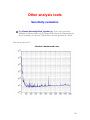
Sensitivity evaluation ................................................................................................................... 129
Sidereal analysis ............................................................................................................................ 132
Data preparation ..................................................................................................................... 132
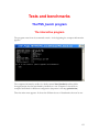
Tests and benchmarks ................................................................................................133
The PSS_bench program............................................................................................................ 133
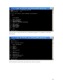
The interactive program ......................................................................................................... 133
The reports ............................................................................................................................... 135
Basic report.......................................................................................................................... 135
FFT report ........................................................................................................................... 136
SFDB ............................................................................................................................................. 138
Hough transform ......................................................................................................................... 138
Service routines ...........................................................................................................139
Matlab service routines ............................................................................................................... 139
pss_lib............................................................................................................................................ 140
pss_rog .......................................................................................................................................... 140
General parameter structure ....................................................................................... 141
Main pss_ structure ..................................................................................................................... 141
const_ structure ........................................................................................................................... 143
source_ structure ........................................................................................................................ 144
antenna_ structure ...................................................................................................................... 145
data_ structure ............................................................................................................................ 146
fft_ structure................................................................................................................................ 147
band_ structure ........................................................................................................................... 148
sfdb_ structure ............................................................................................................................ 149
tfmap_ structure ......................................................................................................................... 150
tfpmap_ structure ....................................................................................................................... 151
hmap_ structure .......................................................................................................................... 152
cohe_ structure ........................................................................................................................... 153
ss_ structure ................................................................................................................................ 154
candidate_ structure ................................................................................................................... 155
event_ structure .......................................................................................................................... 156
computing_ structure ................................................................................................................. 157
The Log Files ..............................................................................................................158
To read logfiles ............................................................................................................................ 161
Example of use of logfile data ................................................................................................... 162
Time events .............................................................................................................................. 163
5
Frequency events..................................................................................................................... 166
The PSS databases and data analysis organization....................................................173
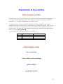
General structure of PSS databases .......................................................................................... 173
The h-reconstructed database .................................................................................................... 175
The sfdb database ........................................................................................................................ 176
The normalized spectra database .............................................................................................. 176
The peak-map database .............................................................................................................. 176
The candidate database ............................................................................................................... 176
The coincidence database ........................................................................................................... 176
Database Metadata ...................................................................................................................... 176
Server docs ............................................................................................................................... 176
Analysis docs............................................................................................................................ 176
Antenna docs ........................................................................................................................... 177
File System utilities ...................................................................................................................... 177
Organization of the workflow ................................................................................................... 178
Basic analysis periods.............................................................................................................. 178
Initial analysis steps ................................................................................................................. 178
hrec extraction .................................................................................................................... 178
sds creation and reshaping ................................................................................................ 178
sfdb creation ........................................................................................................................ 178
peakmap creation................................................................................................................ 178
Main analysis ............................................................................................................................ 179
Data quality.......................................................................................................................... 179
Hough map candidates ...................................................................................................... 179
Final analysis ............................................................................................................................ 179
Coincidence ......................................................................................................................... 179
Coherent analysis ................................................................................................................ 179
Other tasks organization............................................................................................................. 180
Known pulsar investigation ................................................................................................... 180
Known location investigation ............................................................................................... 180
Appendix ..................................................................................................................... 181
Doppler effect computation ...................................................................................................... 181
pss_astro ................................................................................................................................... 181
Theory: Astronomical Times ............................................................................................ 182
Theory: Contributions to the Doppler effect ................................................................. 183
Programming tips ........................................................................................................................ 185
Windows FrameLib ................................................................................................................ 185
Non standard file formats .......................................................................................................... 186
SFDB ........................................................................................................................................ 186
Peak maps ................................................................................................................................ 189
p05 ........................................................................................................................................ 189
p08 ........................................................................................................................................ 196
p09 ........................................................................................................................................ 197
Standard Reports ......................................................................................................................... 198
General ..................................................................................................................................... 198
Data preparation ..................................................................................................................... 199
Candidates ................................................................................................................................ 199
Coincidences ............................................................................................................................ 199
6
Issues ......................................................................................................................................... 199
Matlab procedures (résumé)....................................................................................................... 200
Batch procedures..................................................................................................................... 200
Preparation procedures .......................................................................................................... 200
Check procedures.................................................................................................................... 200
Analysis procedures ................................................................................................................ 201
C procedures (résumé) ................................................................................................................ 202
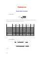
Reference ................................................................................................................... 203
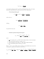
Some basic formulas ................................................................................................................... 203
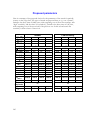
Proposed parameters................................................................................................................... 205
Papers and tutorials ..................................................................................................................... 206
7
Introduction
The PSS software is intended to process data of gravitational antennas to search for periodic
sources.
It is based on two programming environments: MatLab and C. The first is basically oriented
to interactive work, the second to batch or production work (in particular on the Beowulf
farms). There are also programs developed in Matlab, then compiled by the Matlab compiler
and run on the Grid environment.
The input gravitational antenna data on which the PSS software operates can be in various
formats, as the frame (Ligo-Virgo) format, the R87 (ROG) format, or the sds format (that
is one of the Snag-SFC formats). The data produced at the various stages of the processing
are stored in one of the Snag-SFC formats. The candidate database has a particular format.
There are some procedure to prepare data for processing. There is a basic check for timing
and basic quality control. A report is created.
Then the Short FFT Database (SFDB) is created. This is done in different way depending on
the antenna type. For interferometric antennas it is done for 4 bands, obtaining 4 SFDBs.
For bar antennas it is done for a single band.
The SFDB contains also a collection of “very short” periodograms. It has many uses, in
particular it is used for the time-frequency data quality.
From the SFDB the peak map is obtained; it is the starting point for the Hough transform.
The Hough transform (the “incoherent step” of a hierarchical procedure), that is the main
part of our procedure, is normally run on a Beowulf computer farm. A Supervisor program
creates and manages the set of tasks.
The Hough transform produces a huge number (from hundreds of millions to billions) of
candidate sources, each defined by a starting frequency, a position in the sky and a value of
the spin-down parameter. These are stored in a database and when there are independent
data analysis (for different periods or for different antennas), a coincidence search is
performed on them.
The "survived" candidates are then followed-up to verify their compliance with the
hypothesis of being a periodic gravitational source, to refine their parameters and to
compute other (like polarization).
An important part of the package is the simulation modules.
This guides ends with a report of various tests done of some parts of this package.
More information can be found on the programming guides and other documents:
8
Snag2_PG
PSS_PG
PSS_astro_PG
PSS_astro_UG
PSS_Hough_PG
Supervisor_PG
9
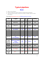
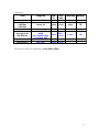
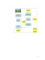
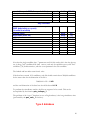
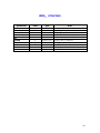
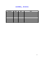
Typical pipelines
Basic
Times are only indicative.
Often the transfer time between computers is higher than processing time.
After each step check and pre-analysis time should be considered (and this could be
much longer).
In the table grid operations are in red, Matlab operations are in blue.
Task
Program
file in
file
out
time/day
Mb/day
hrec
extraction
Extract.tcsh
frame
frame
10 min
1500
frame-tosds
conversion
frame_util
hrec
frame
files
.sds
files
10 min
1400
sds
reshape
sds_reshape
.sds
.sds
15 min
1400
sfdb
crea_sfdb
.sds
.sfdb
30 min
3000
peakmap
crea_peakmap
.sfdb
.p08
15 min
450
p08 to vbl
p082vbl
(by
convert_peakfiles)
.p08
.vbl
30 min
300
cleaning
(mask
creation,
new p08,
new vbl)
clean_conv_peakfile
(using
clean_piapeak)
.vbl
.p08
.vbl
.p08
2 hours
750
input files
creation
create_input_file
.p08
.input
3 min
450
Sky Hough
map
pss_hough
.p08
.cand
4~16
hours
750~3000
(independent
of time)
f/fdot
Hough
map
pss_...
.vbl
.cand
10
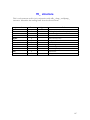
(continuing)
Task
Program
file
in
file
out
time/day Mb/day
single jobs
candidate
collection
create_db
.cand
.cand
4 min
750
psc type 2 db
(50-1050 Hz)
reshape_db2
(using
psc_reshape_db2)
or reshape_db3
.cand
242 x
.cand
1 hour
750
coincidences
psc_coin
.cand
.cand
All batch procedures are submitted by pss_batch_diary.
11
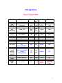
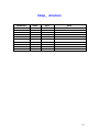
Old pipelines
Up to August 2008
Task
Program
file in
file
out
time/day
Mb/day
hrec
extraction
Extract.tcsh
frame
frame
10 min
1500
frame-tosds
conversion
frame_util
hrec
frame
files
.sds
files
10 min
1400
sds
reshape
sds_reshape
.sds
.sds
15 min
1400
sfdb
crea_sfdb
.sds
.sfdb
30 min
3000
peakmap
crea_peakmap
.sfdb
.p05
15 min
450
p05 to vbl
piapeak2vbl or
(by
convert_peakfiles)
.p05
.vbl
30 min
300
cleaning
(mask
creation,
new p05,
new vbl)
clean_conv_peakfile
(using
clean_piapeak)
.vbl
.p05
.vbl
.p05
2 hours
750
input files
creation
create_input_file
.p05
.input
3 min
450
.cand
4~16
hours
750~3000
(independent
of time)
Hough
map
pss_hough
.p05
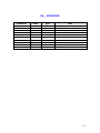
12
(continuing)
Task
Program
file
in
file
out
time/day Mb/day
single jobs
candidate
collection
create_db
.cand
.cand
4 min
750
psc type 2 db
(50-1050 Hz)
reshape_db2
(using
psc_reshape_db2)
or reshape_db3
.cand
242 x
.cand
1 hour
750
coincidences
psc_coin
.cand
.cand
13
Programming environments
Matlab
For the MatLab environment the Snag toolbox is used. It contains more than 800 m
functions (February 2004) and has PSS as one of the projects regarding the gravitational
waves (in snag\projects\gw\pss). It is almost completely independent from other
toolboxes.
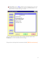
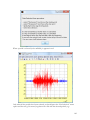
There are two useful interactive gui programs in Snag:
snag , provides a GUI access to the Snag functionalities. It can be used
“stand-alone”, or in conjunction with the normal Matlab prompt use of
Snag. At the Matlab command prompt, type snag . A window appears:
It has a text window, where are listed the gds that have been created and
some buttons.
For a more extensive description of this, see the Snag2_UG.
14
data_browser , that is a Snag application (part of the gw project) to access and
simulate gravitational antennas data. It is started by typing data_browser (or just
db, if the alias is activated). This opens a window
with a text window and some buttons. The text window shows the “status” of the
DataBrowser , as is due to the default and user’s settings.
The parts that are developed in this environment are labeled [MatLab environment].
15
The gw project
Inside Snag, a gravitational wave project has been developed. An important of this project is
the DataBrowser (showed in the preceding sub-section).
Other parts of this project are:
astro , on astronomical computations (coordinate conversion, doppler
computations)
time , with a set of functions dealing with the time. Among the others:
o conversions between mjd (modified julian date), gps and tai times
o sidereal time
o conversions between vectorial and string time formats
sources , about gravitational sources (pulses, chirps and periodic signals)
pss , specifically for the PSS software (see the sub-section)
pulse , regarding pulse detection
gw_sim, with data simulation
radpat , for the radiation pattern and response of antennas (sidereal response of an
antenna, sky coverage,…)
The pss folder
It contains about 200 functions (Feb 2007) divided in :
cohe , for coherent analysis
hough , for Hough transform
hough_exp , containing the Hough Explorer functions
other , service routines, mainly for peculiar file access
procedures , batch procedures
psc , periodic source candidate functions, for analysis and coincidence
sfdb , short FFT database and peak map
16
sim , simulation
theory , statistical and physical theoretical analysis
17
C
The C environment contains a library and some module. The library contains:
pss_snag : routines to operate with the snag objects (GD, DM, DS, RING, MCH)
pss_math : basic mathematical routines
pss_serv : service routine (among the others, vector utilities, string utilities, bit
utilities, interactive utilities, “simple file” management
pss_gw : physical parameters management
pss_astro : astronomical routines
pss_frame : routines for frame format access
pss_r87 : routines for r87 format access
pss_sfc : routines for the sfc file formats management
pss_snf : routines for snf format management (partially obsolete)
The other modules are:
pss_bench : for computer benchmarks
pss_math : basic mathematical routines
pss_sfdb : for short FFT data base and peak maps creation and management
pss_hough : for hough transform
pss_cohe : for the coherent step of the hierarchical search
pss_ss : Hough tasks management and supervision
The parts that are developed in this environment are labeled [C environment].
18
SFC formats
Basics
The basic feature of the file formats here collected is the ease of access to the data.
The "ease of access" means:
the software to access the data consists in a few lines of basic code
the data can be accessed easily by any environment and language
the byte level structure is immediately intelligible
no unneeded information is present
the number of pointers and structures is minimized
the structure fits the needs
the access is fast and, possibly, direct
the need for generality is tempered by the need for easiness.
The collection is composed by:
sds, simple data stream format, for finite or "infinite" number of equispaced samples,
in one or more channels, all with the same sampling time
sbl, simple block data format, in a more general case; a block can contain one or more
data types: any block have the same structure (i.e. the sequence and the format of the
channels is the same) and the same length (i.e. the number of data in a block for a
certain channel, is always the same).
vbl, varying length block data format, where the structure of all the blocks is the same,
but the length can be different.
gbl, general block data format: it is not a format, but practically a sequence of
superblocks, each following one of the preceding formats; it is a repository of data,
not necessary well structured for an effective analysis, but good for storage,
exchange, etc..
A set of files can be:
internally collected, i.e. ordered serially or in parallel using the internal file pointers (for
example subsequent data files, or to put together different sampling time channels)
externally collected, i.e. logically linked by a collection script file, as it happens for
internal collecting
embedded in a single file, with a toc at the beginning or at the end. This is the case of
the gbl files.
A file can be wrapped by adding one or more external headers (for example describing the
computer which wrote the file).
19
The SFC data formats are presented in the Snag2 Programming Guide (Snag2_PG.pdf).
Compressed data formats
These formats are not compulsory (they are not used for the first development phase).
LogX format
This is a format that can describe a real number (float) with little more than 16, 8, 4, 2 or 1 bits. X
indicates this number of bits.
It uses normally a logarithmic coding, but can use also linear coding and, in particular cases, the
normal floating 32-bit format. In the case that all the data to be coded are equal, only one data is
archived (plus the stat variable).
It best applies to sets of homogeneous numbers.
Let us divide the data in sets that are enough homogeneous, as a continuous stretch of sampled data.
The conversion procedure computes the minimum and the maximum of the set and the minimum
and the maximum of the absolute values of the set, checks if the numbers are all positive or negative,
or if are all equal, then computes the better way to describe them as a power of a certain base
multiplied by a constant (plus a sign). So, any non-zero number of the set is represented by
xi = Si * m * bEi
or, if all the number of the set have the same sign,
xi = S * m * bEi
where
Si is the sign (one bit)
m is the minimum absolute value of the numbers in the set
b is the base, computed from the minimum and the maximum absolute value of the
numbers of the set
Ei is the (positive) exponent (15 or 16 bits for Log16, 7 or 8 bits for Log8, and so on).
The coded datum 0 always codes the uncoded value 0 (also if such a value doesn’t exist).
m, b, and a control variable that says if all the number are positive, negative or mixed are stored in a
header. The data bits contain S and E or only E.
The minimum and maximum values can be imposed externally, as saturation values.
In case of mixed sign data, in order to have automatic computation of m and b, an epsval (a
minimum non-zero absolute value) should be defined. If this is put to 0, this value is substituted with
the minimum non-zero absolute datum.
The zero, in the case of mixed sign data, is coded as “111…11”, while “000…00” is the code for the
number m (“1000…00” is –m, “0111…11” is the maximum value and “111…110” the minimum).
20
The mean percentage error in the case of a gaussian white sequence is, in the case of Log16, better
then 10-4 .
Also a linear coding is possible:
xi = m + b * Ei
Also in this case, the coded datum 0 always codes the uncoded value 0 (also if such a value doesn’t
exist).
In case of linear coding, if the data are “mixed sign” (really or imposed) and X is 8 or 16, E is a
signed integer, otherwise it is an unsigned integer: normally, in the first case, m is 0.
In case of data dimension X less than 8 (4, 2 or 1: the sub-byte coding), the logarithmic format is
substituted by a look-up table format. In such case, a look-up table of (2X – 1) fixed thresholds tk
(0<k<2X – 2), in ascending order, must be supplied. Data < t0 are coded as 0, data between tk-1 and
tk are coded as k and data greater than the last threshold are coded as 11..1 . In the case of linear
sub-byte coding, the coded data are unsigned.
Here is a summary of the LogX format:
Number
of bits
32
16
8
4
Coding
float
2 linear
2 logarithmic
2 linear
2 logarithmic
linear
linear
linear
look-up look-up lookup
2
1
0
constant
Logarithmic coding can be done using X or X-1 bits for the exponent, depending if the last bit is
used for the sign. Linear coding can be (for X = 8 or 16) signed or unsigned integer coded.
Linear and logarithmic coding can be adaptive.
So, totally, we have 16 different LogX formats (7 linear, 4 logarithmic, 3 look-up table, 1 float and 1
constant float), 11 of which can be adaptive.
Sparse vector formats
Sparse vector is a vector where most of the elements are 0. We call “density” the percentage
of non-zero elements. Sparse matrixes are formed by sparse vectors.
Sometimes (binary matrices) the non-zero elements are all ones and sometimes they are also
aggregated. In this last case the binary derivative (0 if no variation, 1 if a variation is present)
is often a sparse vector with lower density value.
We represent sparse vectors with the “run-of-0 coding”. It consists in giving just the number
of subsequent zeros, followed by the value of the non-zero element. In the case of binary
vectors, the value of the non-zero element is not reported.
Examples:
{1.2 0 0 0 0 0 3.2 0 0 0 0 0 0 2.3 0 0 0 0 0 0 0 0 3.0 0 0 0 2.}
21
coded as {0 1.2 5 3.2 6 2.3 8 3.0 3 2.}
binary case:
{0 0 0 1 0 0 0 0 0 0 1 0 0 0 0 0 0 0 0 1 1 0 0 0}
coded as {3 6 8 0 3}
aggregate binary case:
{1 1 1 0 0 0 0 0 0 0 0 1 1 1 1 0 0 0 0 0 0 1 1 1 1 1 0 0 0 0 0 0 0 0 0 0 1 1 1}
binary derived as
{1 0 0 1 0 0 0 0 0 0 0 1 0 0 0 1 0 0 0 0 0 1 0 0 0 0 1 0 0 0 0 0 0 0 0 0 1 0 0}
coded as
{0 2 7 3 5 4 9 2}.
In practice the number of subsequent zeroes is expressed by an unsigned integer variable
with b = 4, 8, 16 or 32 bits; one is added to the coded values, in such a way that the value 0
is an escape character used if more than 2n-2 zeroes should be represented; in such case the
datum is put in a side array of uint32.
In practice, there are 5 different cases:
sparse, non-binary
sparse, binary
sparse, derived binary
non-sparse, non-binary
non-sparse, binary
the 0-runs and the non-zero elements
only the 0-runs of the sequence
only the 0-runs of the derived sequence
normal vector (a float per element)
one bit per element
22
PSS SFC files
The PSS (Periodic Source Search) project uses many different types of data to be stored.
Namely:
h-reconstructed sampled data, raw and purged
Short FFT data bases
Peak maps
Hough maps
PS candidates
Events
Each of these has a peculiar type of SFC.
h-reconstructed sampled data, raw and purged
This type of data are normally stored with simple SDS.
Short FFT data bases
The data are stored in a SBL file.
In the user field there are other information like:
[I] FFT length (number of samples of the time series)
[I] Interlacing size (number of interlaced samples)
[D] sampling time of the time series
[S] window (used on the time series)
The blocks contain:
o
o
o
o
one half of the FFT of purged sampled data
one short power spectrum
one one-minute mean vector
a set of parameters as:
1
[I] number of added zeros (for errors, holes or over-resolution)
[D] time stamp of the first time datum (mjd)
[D] time stamp of the first time datum (gps time)
[D] fraction of the FFT time that was padded with zeros
[D] velocity and position of the detector at time of the middle datum1
(vx_eq, vy_eq, vz_eq, px_eq, py_eq, pz_eq: coordinates in Equatorial reference
frame, fraction of c)
Middle datum means the LFFT / 2 1 datum.
23
[D] position of the detector at time the middle datum (x_eq, y_eq, z_eq:
coordinates in Equatorial reference frame, in meters of SSB)
Peak maps
The data are stored in a VBL file. The header is similar to that of the SFDB, but a peak
vector takes the place of the FFT. The format of the peak vector is a sparse binary vector, so
the real length of each block is not constant.
There are two versions of the vbl peak maps, derived from the non-standard format p05 and
p08:
up to August 2008:
There are 3 channels:
- the velocity of the vector (Cartesian, in the Ecliptic reference frame, fraction of c)
- the frequency bins of the peaks (integer)
- the equalized peak values.
starting from August 2008:
There are 5 channels:
- the velocity of the vector (Cartesian, in the Ecliptic reference frame, fraction of c)
- the short spectrum
- the index of the peaks array (for direct access to PEAKBIN)
- the frequency bins of the peaks (integer; can be negative for vetoed peaks)
- the equalized peak values.
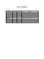
The channels have the following parameters:
CH
name
lenx
dx
type
1
DETV
3
double
2 SHORTSP length of short spectrum sh.sp. frequency step float
3
INDEX
length of short spectrum sh.sp. frequency step
int
4 PEAKBIN
length of half FFT
FFT. frequency step
int
5
PEAKCR
float
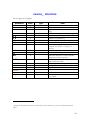
starting from November 2010:
There are 6 channels:
- the velocity of the vector (Cartesian, in the Ecliptic reference frame, fraction of c)
- the short spectrum
- the index of the peaks array (for direct access to PEAKBIN)
- the frequency bins of the peaks (integer; can be negative for vetoed peaks)
- the equalized peak values.
- the mean for the peaks
24
The channels have the following parameters:
CH
name
lenx
dx
type
1
DETV
3
double
2
SHORTSP
length of short spectrum sh.sp. frequency step float
3
INDEX
length of short spectrum sh.sp. frequency step
int
4
PEAKBIN
length of half FFT
FFT. frequency step
int
5
PEAKCR
float
6 PEAKMEAN
float
Hough maps
The data are stored in SBL or VBL files. The parameter to be stored in each block
(containing a single Hough map) are:
the length of the record
the parameters of the hough map (amin, da, na, dmin, da, nd)
the spin down parameters (nspin, spin1,spin2,…)
the number of used periodograms and the type (interlaced, windowed,…)
the initial times and length of each periodogram
the type and the parameters of the threshold
PS candidates and Events
These data could be stored in an SDS file, with many channels, but, for the
necessity of easy random access needed for such data bases, a peculiar format
will be used.
25
Data preparation
Format change
[C environment]
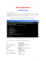
In order to use some Snag features in a more proficient way, the frame format data must be
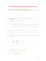
must be converted in the sds format. This can be accomplished by the interactive program
FrameUtil.exe. It can be run in two ways: interactive or batch:
Interactive (can be used also in batch mode in some systems)
Very useful are the two dump file facilities, that give a resume of all the frames.
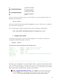
The program can be used also in batch, creating a batch file as this:
8
1
1
/home/federica/hrec-v2/
3
dL_20kHz
4
hrec
5
/home/federica/sds/
2
! ask batch mode
! sets batch mode
! ask item choice of the directory
! input directory
! ask channel choice
! channel
! ask item DataType file name block
! the block
! ask output directory
! output directory
! ask item File choice
hrec-710517600-3600.gwf
6
! the file
! creates the sds file
26
2
hrec-710521200-3600.gwf
6
2
hrec-710524800-3600.gwf
6
12
! ask item File choice
!
! creates the sds file
! ask item File choice
!
! creates the sds file
! exit
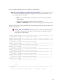
To create easily the batch file, create a list of the files to be converted and then edit it. In
Windows the command is
dir /b > list.txt
and can be issued with the command file to_list.bat ; it creates a file list.txt, to be edited to
create the batch command file.
To start the program a batch command can be created containing something like
D:\SF_Prog\C.NET\FrameUtil\Release\frameutil < batchwork.txt > out.txt
Simple batch mode
Alternatively the program can be run with the argument of a text file that contains the
configuration and the file names, in this way:
> frameutil
batch.txt
The text file (any name is possible) has the following format:
folder in
folder out
channel
antenna acronym
data type
frame file1
frame file2
frame file3
...
example:
example:
example:
example:
example:
example:
D:\Data\pss\virgo\sd\frame\
D:\Data\pss\virgo\sd\sds\
h_4kHz
VIR
hrec
HrecV-806888400-01-Aug-2005-01h40-600F.gwf
-------------------------------------------------------------------------------------------------------If we have a set of sds files, we can "concatenate" them, i.e. put in each of them the correct
values for filspre and filspost, so the data can be seen as a continuous stream, and one can
access at any of them pointing to any file of the chain (also not containing the given datum).
This concatenation is performed, for example, by the function
sds_concatenate(folder,filelist) , where folder is the folder containing the
files and filelist a file containing the file list (similar to the above list.txt) in the
correct order. Be sure that the files in the list are in the correct order !
27
A more complex operation on a set of sds files is performed by
sds_reshape(listin,maxndat,folderin,folderout) , that constructs a new set
of sds files with different maximum length and concatenates them. In this way a
more efficient data set is built.
o listin is a file containing the file list (similar to the above list.txt) in the
correct order
o maxndat is the maximum number of data for a channel
o folderin and folderout are the folders containing the input and output data
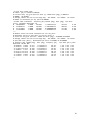
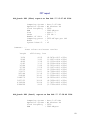
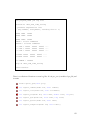
When all the files of a run are produced and concatenated (possibly with sds_reshape), they
should be checked by
check_sds_conc(outfile) , that analyzes the set of files, producing a report
in outfile (or on the screen, if outfile is absent). Here is an example of one of
these reports (c5-data.check):
VIR_hrec_20041203_004502_.sds 03-Dec-2004 00:45:02.000000
h_4kHz - err = 0.000000
1598.000000 s --> HOLE at 03-Dec-2004 01:48:12.000000
VIR_hrec_20041203_021450_.sds 03-Dec-2004 02:14:50.000000
h_4kHz - err = 0.000000
VIR_hrec_20041203_054310_.sds 03-Dec-2004 05:43:10.000000
h_4kHz - err = 0.000000
50.000000 s --> HOLE at 03-Dec-2004 06:15:39.000000
VIR_hrec_20041203_061629_.sds 03-Dec-2004 06:16:29.000000
h_4kHz - err = 0.000000
13172.000000 s --> HOLE at 03-Dec-2004 07:31:19.000000
VIR_hrec_20041203_111051_.sds 03-Dec-2004 11:10:51.000000
h_4kHz - err = 0.000000
57.000000 s --> HOLE at 03-Dec-2004 11:25:32.000000
VIR_hrec_20041203_112629_.sds 03-Dec-2004 11:26:29.000000
h_4kHz - err = 0.000000
23392.000000 s --> HOLE at 03-Dec-2004 11:39:52.000000
VIR_hrec_20041203_180944_.sds 03-Dec-2004 18:09:44.000000
h_4kHz - err = 0.000000
106.000000 s --> HOLE at 03-Dec-2004 18:22:40.000000
VIR_hrec_20041203_182426_.sds 03-Dec-2004 18:24:26.000000
h_4kHz - err = 0.000000
51.000000 s --> HOLE at 03-Dec-2004 21:02:00.000000
VIR_hrec_20041203_210251_.sds 03-Dec-2004 21:02:51.000000
h_4kHz - err = 0.000000
42.000000 s --> HOLE at 03-Dec-2004 21:03:06.000000
duration: 3790.000000 s
chs:
duration: 12500.000000 s
chs:
duration: 1949.000000 s
chs:
duration: 4490.000000 s
chs:
duration: 881.000000 s
chs:
duration: 803.000000 s
chs:
duration: 776.000000 s
chs:
duration: 9454.000000 s
duration: 15.000000 s
chs:
chs:
………………………………………………………
Summary
133 files start: 03-Dec-2004 00:45:02.000000
3.571748 days
129 holes
of total duration 141025.000000 s
end: 06-Dec-2004 14:28:21.000000
Tobs =
percentage = 0.456985
28
Data selection
[MatLab environment]
Basic sds operations
If the sampled data are in the sds format, it is easy to perform a variety of tasks. Here we will
speak of higher level tasks (lower levels are discussed in the programming guides). Among
the others, of particular interest for the PSS :
sfc_=sfc_open(file) , that outputs the sfc structure of the file
[chss,ndatatot,fsamp,t0,t0gps]=sds_getchinfo(file) , that shows the UTC
time and outputs channels (in a cell array), the total number of data, the sampling
frequency and the initial time both in MJD (modified julian date) and gps.
g=sds2gd_selt(file,chn,t) , creates a gd from file, channel number chn and t =
[initial time, duration]; if the parameters are not present, asks interactively.
sds_spmean(frbands,file,chn,fftlen,nmax) , creates an sds file, named
psmean.sds, containing the spectral means for many different bands. frbands is an
Nx2 matrix containing the bands; if it is not present, it can be input as a text file like,
for example,
0 20
20 48
48 52
52 70
70 98
98 102
102 200
200 500
500 1000
1000 2000
file and chn are the file and the channel number, fftlen is the length of the FFT and
nmax the maximum number of output data (put a big number and all the
concatenated files will be analyzed).
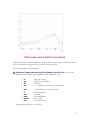
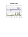
m=sds2mp(file,t) , creates an mp (multi-plot structure) from an sds file (the
command can be issued without parameter and asks interactively). For example, it
can be applied to the spectral mean sds file created by sds_spmean. The mp
structure can be showed by mp_plot(m,3) (m is the mp and 3 means log y),
obtaining (on E4 data of the CIF)
29
or else (among other choices)
The abscissa is in hours from the 0 hours of the first day.
crea_ps(sdsfile,chn,lfft,red) , creates an sbl file containing power spectra of
data (similar to that produced for the sfdb), from channel number chn, a "big FFT
length" lfft and a length of the power spectra lfft/red.
30
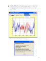
Choice of periods
[MatLab environment]
The choice of the periods on which the SFDB should be created (and then are to be
analyzed) can be done by the use of the Virgo data quality information and of the basic
instruments like those shown in the preceding section.
In Snag there are some useful interactive functions that helps in choosing prtiods:
xx=sel_absc(typ,y,x,file) , the easyest one, where typ (0,1,2,3) indicates the type
of plot (simple, logx, logy, logxy), y is a gd or an array, x is simply 0 (if y is a gd) or
the abscissa array, file (if present) is the file to put the output, i.e. the starting and
ending points of the chosen periods; xx is an (n,2) array with the bounds of the
chosen periods. This program is very simple to use: you can directly choose the start
and stop abscissa of as many periods you want; when you chose the stop point, the
chosen period is colored in red and you are prompted if you choose another period
The problem with this function is that it is not possible to zoom the plot for more
precise choice.
31
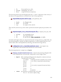
sel_absc_hp(typ,y,x) , permits the use of the zoom and so an high precision
choice. It uses global variables (ini9399, end9399, n9399 as the beginning times,
ending times and number of periods); The data of the periods are put in a file
named fil9399.txt. The input variables typ, y and x have the same use of the
function sel_absc.
There are some easy rules that appear at beginning:
32
Search for events
[MatLab environment]
Filtering in a ds framework
The ev-ew structures
The event management is done by the use of the ev-ew Snag structure (see the
programming guide Snag2_PG.pdf). An event is defined by a set of parameters, like
o
o
o
o
o
o
o
the (starting) time of the event (in days, normally mjd)
the time of the maximum (in days, normally mjd)
the channel
the amplitude
the critical ratio
the length (in seconds)
…
The difference between the ev and ew structures is that the first describes a single event (so
a set of events is an array of structures), the second describes a set of events. The ew
structure is normally more efficient, but the ev structure is more rich (it can contain also the
shape of the event). The two function ew2ev and ev2ew transform one type in the other
(losing the shape, if present).
A set of events is associated to a channel structure that describes the channels that produced
the events, constituting a new event/channel structure evch.
There is a number of auxiliary functions to manage events:
chstr=crea_chstr(nch) , creates a channel structure for events; nch is the
number of channels
evch=crea_ev(n,chstr,tobs) , creates an event-channel structure, simulating n
events in the time span tobs, and with the channel structure chstr
evch=crea_evch(chstr,evstr) , creates an event-channel structure, from a
channel structure and an event structure
[fil,dir,fid]=save_ech(ch,direv,fil,mode,capt) , save a channel structure in an
ascii file that can be edited; ch is the channel structure, direv and fil are the default
folder and file, mode is 0 for standard, 1 for the full evch, capt is the caption
[fil,dir]=save_ev(ev,direv,fil,mode,fid,capt) , save an event structure in an
ascii file that can be edited; ev is the event structure, direv and fil are the default
33
folder and file, mode is 0 for standard, 1 for the full evch, fid is the file identifier (or
0), capt is the caption
save_evch(evch) , saves an evch structure in Matlab format
load_evch , interactively loads an evch structure in Matlab format
eo=sort_ev(ei) , time sorts an event structure
out=ev_sel(in,ch,t,a,l) , selects events on the basis of the channel, time
occurrence, amplitude and length.
o
in and out are the input and output evch structure,
o ch , if it is an array, it is the probability selection of different channels (if < 0,
the channel disappear), otherwise is not used;
o t, a, l , if it is an array of length 2, defines the interval of acceptance; if the
first element is greater than the second, they defines the interval of rejection
chstr=stat_ev(evch) , statistics for events
dd=ev_dens(evch,selch,dt,n) , event densities;
o evch event/channel structure
o selch selection array for the channels (0 exclude, 1 include)
o dt time interval
o n number of time intervals
ev_plot(evch,type) , plots events. type is:
0.
1.
2.
3.
4.
5.
6.
simple
amplitude colored
length colored
both
stem3 amplitude
stem3 length
stem3 both
Coincidences
To study coincidences between events a set of functions is provided:
[dcp,ini3,len3,dens] = ev_coin(evch,selch,dt,n,type,coinfun) , creates a
delay coincidence plot (dcp) and finds coincident events (ini3, len3 are the initial
times and lengths, dens is the event density, if used). In input:
o evch is an event/channel structure
34
o selch is a selection array, with the dimension of the number of channels, that
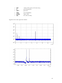
defines which channels are to be put in coincidence: every channels can be
0 excluded
1 put in the first group
2 put in the second group
3 put in both
o dt is the time resolution (s)
o n is the number of delays for each side
o type an array indicating the coincidence type:
type(1) : 1 only event maxima
2 whole length coincidences
type(2) : 1 normal
2 density normalized
type(3) : density time scale (s) for density normalization
o coinfun if exists, external coincidence function is enabled. The coincidence
function is > 0 if the events are "compatible"; the inputs are
(len1,len2,amp1,amp2), that are the lengths and amplitudes for the two
coincident event.
It produces the plot of the delay coincidences and its histogram.
[dcp,in3,len3]=vec_coin(in1,len1,in2,len2,dt,n,coinfun,a1,a2) , is one of
the coincidence engines used inside ev_coin. It considers the length of the events
[dcp,in3]=vec_coin_nolen(in1,in2,dt,n,coinfun,a1,a2) , is one of the
coincidence engines used inside ev_coin. It considers the length of the events as
dt.
ch=ev_corr(evch,dt,mode) , computes and visualize the correlation matrix
between all the channels. mode = 1 is for symmetric operation, mode = 0 is for
"time arrow" coincidence (causality). It produces also the map of the matrix.
evcho=cl_search(evchi,dt) , identifies cluster of events and labels the events
with the cluster index
Event periodicities
An important point in the event analysis is the study of periodicities. This is performed by
the following functions:
sp=ev_spec(evch,selev,minfr,maxfr,res) , that performs the event
spectrum; in input we need:
35
o
o
o
o
o
evch event/channel structure
selch channelt selection array (0 excluded channel)
minfr minimum frequency
maxfr maximum frequency
res
resolution (minimum 1, typical 6)
pd=ev_period(evch,selch,dt,n,mode,long,narm), event periodicity study
(phase diagram); in input we need:
o evch event/channel structure
o selch channel selection array (0 excluded channel)
o dt
period
o n
number of bins of the phase diagram (pd)
o mode = 0 simple events
= 1 density normalization; mode(1) = 1, mode(2) = bin width (s)
= 2 amplitude; mode(1) = 2, mode(2) = 0,1,2 (normal, abs, square)
o long longitude (for local periodicities (local solar and sidereal)
o narm number of harmonics
36
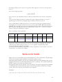
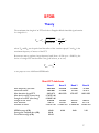
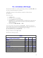
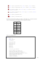
SFDB
Theory
The maximum time length of an FFT such that a Doppler shifted sinusoidal signal remains
in a single bin is
Tmax
c
1.1105
TE
s
4 2 RE G
G
where TE and RE are the period and the radius of the “rotation epicycle” and nG is the
maximum frequency of interest of the FFT.
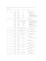
Because we want to explore a large frequency band (from ~10 Hz up to ~2000 Hz), the
choice of a single FFT time duration is not good because, as we saw,
Tmax G
1
2
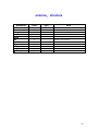
so we propose to use 4 different SFDB bands:
Short FFT data base
Max frequency per band
Observed bands
Max duration for an FFT
Max len for an FFT (max freq)
Length of an FFT (max freq)
Length of the FFTs
FFT duration
Number of FFTs
Band 1
2000.0000
1500.0000
2445.6679
9.7827E+06
8.3886E+06
8388608
2097.15
9.5367E+03
SFDB storage (GB)
Storage for sampled data (GB)
Total disk storage (GB)
160.00
80.00
292.50
Band 2
500.0000
375.0000
4891.3359
Band 3
125.0000
93.7500
9782.6717
Band 4
31.2500
23.4375
19565.3435
4194304
4194.30
4.7684E+03
2097152
8388.61
2.3842E+03
1048576
16777.22
1.1921E+03
40.00
10.00
2.50
37
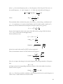
Procedure
o apply a frequency domain anti-aliasing filter and sub-sample (if 20 kHz data)
o high events identification and removal
o create a stream with low and high frequency attenuation
o identify the events on this stream (starting time and length) with the adaptive
procedure. After this, this stream is no more used.
o smooth removal of the events in the original stream (purged stream)
o estimate the power of the purged stream every minute (or so), creating the
PTS (power time series)
o for each of the 4 sub-bands of the SFDB :
o (not for the first band) apply anti-aliasing and subsample
o create the (windowed, interlaced) FFTs, both simple and double resolution:
the simple resolution are archived for the following steps, the double is used
for the peak map
o create a low resolution spectrum estimate (VSPS - Very Short Power
Spectrum, e.g. length 16384)
38
Software [C environment]
Routines
pss_sfdb
39
Software [MatLab environment]
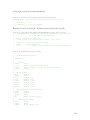
There is also a software to create a SFDB using Matlab. This can be used for checking and
particular purposes.
crea_sfdb(sdsfile,chn,lfft,red) , can be used also interactively without
arguments; sdsfile is the first sds file to be processed, chn is the channel number,
lfft is the length of the (non-reduced) ffts, red is the reduction factor for the
requested band (normally 1, 4, 16, 64). A file sfdb.sbl is created, with the fft
collection.
There are also some useful routines:
iok=piaspet2sbl(folder,piafilelist,filesbl) , extracts the “very short” spectra
from the Pia SFDB files.
folder
piafilelist
filesbl
folder containing the input pia files
pia file list (obtained with dir /b > list.txt)
file sbl to create
40
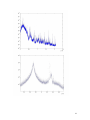
Time-frequency data quality
[MatLab environment]
The time-frequency data quality analysis is done using
a) the set of power spectra created together with the SFDB
b) the set of power spectra created by the function crea_ps
c) the high resolution periodograms obtained directly from the SFDB FFTs
In the cases a) and b), the time-frequency map can be imported in a gd2 with the function
g2=sbl2gd2_sel(file,chn,x,y) , where file is the sbl file containing the power
spectra (for example, an sfdb file), chn the channel number in the sbl file, x a 2
value array containing the min and the max block, y a 2 value array containing the
min and the max index of the spectrum frequencies
From this gd2 an array can be extracted and on it the map2hist and imap_hist can be
applied:
[h,xout]=map2hist(m,n,par,linlog) , creates a set of histograms, one for each
frequency bin, of the various spectral amplitudes of that bin at all the times. m is the
time-frequency spectral map, n is the number of bins for the histograms, linlog (=
0,1) determines if the histogram is done on the value spectral values of the spectra
or on their logarithms, par is the set of parameters to do the histograms:
o if m is an mx2 array, it contains the min and the max of the histograms
o if m = 0, the bounds of the histograms are computed automatically by taking
the minimum and the maximum of all the data
o if m = 1, the bounds of the histograms are computed automatically by taking
the minimum and the maximum of every bin.
imap_hist(h,x,y) , is used to plot the histogram map; h is the histogram map, x is
the frequency value, y the spectral values (if the scale is unique). Here are the two
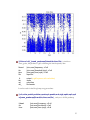
maps for the two cases of par=0 and par=1.
41
42
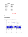
Peak map
From the SFDB we can obtain the "peak map", i.e. a time-frequency map containing the
relative maxima of the periodograms built taking the square modulus of the short FFTs.
To obtain the peak map, the procedure is the following:
o read a short FFT of the data from the database
o using this, construct an enhanced resolution periodogram
o equalize the periodogram, using, for example, the ps_autoequalize procedure
o find the maxima of the equalized spectrum above a given threshold (for
example 2)
The stored data can be just 1 and 0 (binary sparse matrix) or also the values of the maxima
of the not equalized spectra (this in order to evaluate the "physical" amplitude (instead of the
"statistical" amplitude).
The format of the file can be sbl or vbl, depending if a normal or compressed form is
chosen. The peak map file contains all the side information of the SFDB "parent" file.
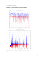
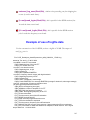
Peak map creation
[MatLab environment]
The peak map can be created by
crea_peakmap(sblfil,thresh,typ) , where sblfil is the SFDB file, thresh is the
threshold and typ is the type (0 normal with amplitudes, 1 compressed with
amplitudes, 2 normal only binary, 3 compressed only binary). Here there is an image
of the peak data (with zooms):
43
44
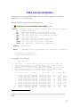
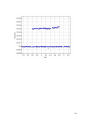
Other peak map creation procedures
Various techniques have been studied to construct effective peak maps. The main problem is
that of the presence of big peaks, that “obscure” the area around.
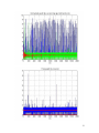
The basic procedure is the following:
[ind,fr,snr1,amp,peaks,snr]=sp_find_fpeaks(in,tau,thr,inv), based on the
gd_findev function idea, that is adaptive mean computation, with
o
o
o
o
o
o
o
o
o
o
o
in
tau
thr
inv
input gd or array
AR(1) tau (in samples)
threshold
1 -> starting from the end, 2 -> min of both
ind
fr
snr1
amp
peaks
snr
index of the peak (of the snr array)
peak frequencies
peak snr
peak amplitudes
sparse array
the total snr array
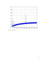
Applying this procedure to a plot like
45
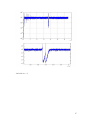
We have, with inv=0,
46
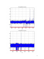
And with inv = 2,
47
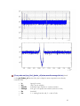
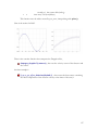
[i,fr,s,peaks,snr]=sp_find_fpeaks_nl(in,tau,maxdin,maxage,thr,inv), based
on the gd_findev_nl function idea, that is adaptive mean computation non-linearly
corrected, with
o
o
o
o
o
o
o
in
tau
maxdin
maxage
thr
inv
input gd or array
AR(1) tau (in samples)
maximum input variation to evaluate statistics
max age to not update the statistics (same size of tau)
threshold
1 -> starting from the end, 2 -> min of both
48
o
o
o
o
o
o
ind
fr
snr1
amp
peaks
snr
index of the peak (of the snr array)
peak frequencies
peak snr
peak amplitudes
sparse array
the total snr array
Applied to the same spectrum obtains:
49
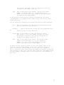
Rough cleaning procedure
These procedure is setup to eliminate spurious lines. It is based only on the peak frequency
histogram.
cd d:\data\pss\virgo\pm\c6
>> [spfr,sptim,peakfr,peaktim,npeak,splr,peaklr,mub,sigb]=…
ana_peakmap(0,0,0,0,'peakmap-c6_1.vbl');
>> mask=crea_cleaningmask_old(peakfr,5,1.6181);
>> clean_piapeak(mask,'peakmap-c6_1.dat');
>> piapeak2vbl(4000/4194304,4194304,…
'peakmap-c6_1_clean.dat','peakmap-c6_1_clean.vbl')
50
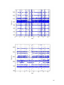
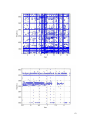
Frequency domain cleaning procedure
These procedure is based on the frequency histogram of peaks and the a priori knowledge
on lines.
The basic function is
mask=crea_cleaningmask(peakfr,nofr,nomfr,yesfr,thrblob,thratt) ,
with
peakfr
nofr
nomfr
yesfr
thrblob
thratt
peakfr (peak frequency histogram) gd
excluded frequencies; mat[nfr,3] with (centr. freq, band,
att.band) 0 -> no, <0 -> only attention band
excluded frequencies and harmonics; mat[nfr,3] with
(centr. freq, band, att.band). 0 -> no
not excluded frequencies; mat[nfr,2]
with (centr. freq,band). 0 -> no
threshold on unexpected blobs (def = 1.2)
threshold on attention band (def = 1.6)
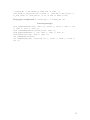
An example of use is by the procedure crea_mask :
% crea_mask
[spfr,sptim,peakfr,peaktim,npeak,splr,peaklr,mub,sigb]=ana_peakmap(0,0,
0,0,'peakmap-C7.vbl');
nofr=read_virgolines(10,2000);
[nl,i2]=size(nofr)
nofr(nl+1,1)=950;
nofr(nl+1,2)=-1;
nofr(nl+1,3)=6;
nofr(nl+2,1)=1002;
nofr(nl+2,2)=-1;
nofr(nl+2,3)=4;
nofr(nl+3,1)=1340;
nofr(nl+3,2)=-1;
nofr(nl+3,3)=10;
mask=crea_cleaningmask(peakfr,nofr,[[10 0 1];[99.1886 0 0.01]],0);
The read_virgolines function reads a lines file in Virgo format.
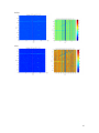
crea_cleaningmask produces also figures to check the mask creation:
51
52
53
Peak map analysis
In a “old” vbl-file the first channel is the parameters (as the detector velocity in AU/day),
the second the frequency bins number, the third the equalized amplitudes; other channels
can contain short spectra and other.
In the “new” vbl-file the first channel is the parameters (as the detector velocity normalized
to c), the second the short spectrum, the third the index for the peak vector, the fourth the
peak vector, i.e. the frequency bins number, the fifth the equalized amplitudes.
To take the data of the peak map, the following function can be used:
[x,y,z,tim1]=show_peaks(frband,thr,time,file) , where
frband
thr
time
file
[min,max] frequency; =0 all
[min,max] threshold (mjd); =0 all
[min,max] time (mjd); =0 all
input file
x,y,z
peaks data (time,frequency,amplitude)
It shows also the plot of the x,y points.
54
[A tim vel vbl_]=read_peakmap(frband,thr,time,file) , is similar to
show_peaks, but produces a gd2 containing the time-frequency data:
frband
thr
time
file
[min,max] frequency; =0 all
[min,max] threshold (mjd); =0 all
[min,max] time (mjd); =0 all
input file
A
tim
vel
vbl_
output (a gd2 sparse, with velocities)
times
velocities
file header
It can be used for the Hough map snag procedures.
[crfr,crtim,peakfr,peaktim,npeak,splr,peaklr,mub,sigb,sphis,spfr,spti
m]=ana_peakmap(frband,thr,time,res,file) , analyzes a vbl-file peakmap.
frband
thr
time
[min,max] frequency; =0 all
[min,max] threshold; =0 all
[min,max] time (mjd); =0 all
55
res
low-res
file
resolution reduction in frequency in low-res maps; =0 no
input file
crfr,crtim
mean cr vs freq and time
spfr,sptim
mean spectrum vs freq and time
peakfr,peaktim number of peaks vs freq and time
splr,peaklr
t-f peak maxima and number (low-res)
sphis
peak CR histogram
mub,sigm
mean,std of peaks in a spectrum
npeak
total number of peaks
56
Time-frequency cleaning
The idea is to histogram the peak map in a lower resolution 2D-grid (for example 12 h
starting from 6 for time and 0.01 Hz for frequency), then define the maximum allowable
value of this histogram for the “normal data” (e.g. 80) and finally cut away the peaks in notallowable spots. The cut-away procedure simply change to negative the sign of the
frequency of the peaks.
In practice the procedure, starting from the “dirty” vbl, is the following:
create the peakmap file list with e.g.: dir *.vbl /s/b > list_VSR2_pm.txt and edit
to eliminate blank lines etc.
edit and execute ana_peakmap_basic.m: this creates the PMC files (peakmap
maps).
This should be done for 5~8 sub-bands each time
create the PMH files list
edit and execute ana_PMH, fixing the threshold thresh: this creates the veto
array and the vetocell cell array
apply tfclean_vbl; this creates the new vbls, that have anyway the full information
of the cut peaks
concatenate new vbl files (if needed) with conc_vbl
check the effect with ana_peakmap_basic_cl.m .
Functions:
Script:
tfclean_vbl
read_peakmap
integralF_fromhist
plot_peaks
p2rgb
p2rgb_colormap
color_points
ana_peakmap_basic and ana_peakmap_basic_cl
% ana_peakmap_basic
Dfr=5;
VSR='VSR4'; % EDIT
for i = 17:26 % EDIT
band=[(i-1) i]*Dfr;
strtit=sprintf(' %s band %4.1f - %4.1f',VSR,band)
savestr=sprintf('PMH_%s_%03d_%03d',VSR,band);
57
eval(['[A tim vel vbl_]=read_peakmap(''list_' VSR
'_pm.txt'',band,0,0);'])
eval(['[x y v ' savestr ']=plot_peaks(A,1,0,1,strtit);'])
eval(['save(''' savestr ''',''' savestr ''');'])
end
ana_PMH Analyzes PMH and creates time-frequency veto structures
conc_vbl concatenates vbl files
58
Effectiveness of the procedure on peakmaps
(Using check_PMH)
Resolution 12 hours/0.01 Hz. Threshold 80
On VSR2 (blue all, red clean):
241748723 all peaks, 206402619 cleaned; perc 0.853790
59
On VSR4 (blue all, red clean):
122104240 all peaks, 102300423 cleaned; perc 0.837812
Important: it doesn’t cancel gravitational signals. Case of the Pulsar 3:
60
before:
after:
61
Hough transform (“classical”)
[C environment]
Introduction ................................................................................................................. 62
Theory .......................................................................................................................... 62
Implementation ........................................................................................................... 63
Function prototypes ..................................................................................................... 69
User assigned parameters ............................................................................................ 70
Performance issue ........................................................................................................ 71
Results of gprof.............................................................................................................................. 71
Comments ...................................................................................................................................... 76
Appendix ...................................................................................................................... 77
crea_input_file................................................................................................................................ 77
create_db......................................................................................................................................... 77
Introduction
This is the User Guide for the PSS_hough library.
PSS_hough is a C library which performs the first (full-sky) incoherent step in the
hierarchical procedure developed by the Virgo Rome group for the search of periodic
gravitational signals in the data of the Virgo interferometer. The input consists of a peak
map file, the output of a candidate file.
For performance reason, the program does not use as input the whole peak map produced
in the preceding step of the analysis but small portions of the peak map which are produced
at the beginning with the program crea_input_file which is described in the Appendix.
Once the candidates have been produced they are organized in a candidate database through
the program create_db which is also described in the Appendix..
Theory
The Hough transform is a robust parameter estimator for patterns in digital images.
It can be used to estimate the parameters of a curve which best fits a given set of points.
The basic idea is that of mapping the data into the parameter space and identifying the
For instance, suppose our data are distributed as a straight line: y=m*x+q. In this case the
parameters to be determined are the slope m and the intercepta q. To each point (x,y) a new
straight line in the parameter space with equation q=y-m*x corresponds. That is, we can
draw a line in the parameter space for each pair (x,y) and all these will intersect in a point
(m,q) identifying the parameters of the original line. If noise is present several “clusters” of
points will appear in the parameter space.
In our case, the original data are the points in the time-frequency peak map and the
62
transformed data are points in the source parameter space: , , f 0 , f0 , f0,... i.e. source
position, frequency and frequency derivatives.
Assuming that there is no spin-down, the relation among each point in the time-frequency
plane and the points in the parameter space is given by the Doppler effect equation
v n
fk f0 f0
c
where f k is the frequency of a peak, v is the detector velocity vector and n is the versor
identifying the direction of the source. From this equation we find that the locus of points in
the sky to which a source emitting a signal at frequency at f 0 could belong, if a peak at
frequency f k is found, is a circle with radius given by
fk f0
v
f0
c
and centered in the direction of the detector velocity vector.
Due to the frequency discretization, in fact we have an “annulus”, delimited by two circles
Peaks belonging to the same spectrum produce concentric annuli, while moving from one
spectrum to the following the center of the annuli moves on the celestial sphere around the
ecliptic. Moreover, also the circles radius changes in time, because of the variation of the
modulus of the detector velocity vector.
For a given value of the source reference frequency f 0 and spin-down, calculating the annuli
corresponding to all the peaks in the time-frequency map and properly summing them, in
order to take into account the source spin-down, we compute the Hough map.
For each value of the source reference frequency we have several Hough maps, depending
on the number of possible different values of the spin-down parameters.
The number of spin-down parameters that must be taken into account depends on the
f
minimum source decay time, 0 , which we search for. In order to limit the overall
f0
cos k
needed computing power to a reasonable value, min ~ 10 4 yr could be a reasonable choice
for the analysis of the whole frequency band over months. This would imply that
only the first spin-down parameter should be considered. For shorter observation period,
like C6 or C7 Commissioning Runs we can adopt a smaller value for the minimum decay
time.
The total number of Hough maps that are built is given by the product of the number of
frequencies to be searched for and of the number of values of the first order spin-down
parameter. N f 0 N f0 . On each map a number of candidates is selected putting a suitable
threshold.
Implementation
Pss_hough is divided in the following files:
pss_hough_drive.c: module containing the main function and all the functions
which are common (at most modulo the data type of the hough map and hough map
63
derivative) to “standard” and adaptive hough transform: parameters computation,
construction of the LUT, reading of the peakmap input file, selection of candidates.
pss_hough.h: header file containing type definitions, global variable declarations,
function prototypes, constants, declaration of structures.
pss_hough.c: module containing functions related to the computation of the
“standard” Hough transform.
pss_hough_adaptive.c: module containing functions related to the computation
of the adaptive Hough transform.
Makefile, MakefileAdaptive: makefiles for compiling and linking the library
respectively for the “standard” and adaptive Hough transform.
The library can be divided, from a logical point of view, into four parts.
–
Building of the Look Up Table (LUT).
For each search frequency a new LUT is computed (As a matter of fact, the
same LUT could be used for more frequencies but for the moment – i.e. as
long as observation times are short and then computing times are not too
much long - we take a “conservative” approach). Given a search frequency
and a spin-down value, we use the same LUT for all the times for which the
frequency shift respect to the original one is lower than a given number of
frequency bin, 4 in our current default choice. This value is somewhat
arbitrary and again conservative: it can be shown that using the LUT for 27
different frequency bins would be enough, and even more at low frequencies.
Given a frequency, the circles corresponding to all the possible peaks in the Doppler
band of the chosen frequency are computed. The ecliptic coordinate system is used. As a
consequence, the circles have centers in a narrow belt around the ecliptic. This belt is
discretized so that ordinates of the circle centers are taken in a discrete set (of 11 different
values) while the abscissa is assumed to be zero. Also the sky is discretized in a number of
pixels, then two circles with the same center are distinguishable only if their radii differ by
at least one pixel.
For each circle center and for each allowed radius, there is a loop on the ordinate values
and, correspondingly, the values of the abscissa (as real values) only for the left semicircle are computed. This is done for performance reasons, since it is then very simple to
determine the corresponding right semi-circle using simmetry arguments.
The computed abscissae are stored into an array which is the look-up table. Another array
is created, containing the index (along the vertical direction) of the pixels corresponding
to the minimum and the maximum ordinate of each circle and cumulative difference
between them.
–
Reading of the peak map
For each time read the portion of the peak map input file corresponding to the Doppler
band around the actual frequency (which takes into account the spin-down). Each read
peaks is “translated” into one or more peaks of the LUT: in this way we take into account
the fact that the LUT circles are computed for the largest possible velocity and then are
64
more numerous than the “true” ones (i.e. it may be possible that one peak of the peak
map corresponds to two circles of the LUT).
–
Calculation of the Hough Map (HM).
The HM is a histogram in the sky coordinates. For each selected peak, two semi-circles
are read from the LUT: one corresponding to the current peak and one corresponding to
the peak immediately before (in the LUT). This is done because each peak, in a
discretized space, produces an annulus of pixels, delimited by a pair of circles. The center
of each semicircle is properly shifted, depending on the time index, and the
corresponding right half is computed using simmetry; then for each peak we have four
semicircles. Semicircles with radius larger than 90 degrees are computed taking the
corresponding “opposite” circles with lambda rotated by 180 degrees and beta inversed.
To the pixels of the semicircle of each pair (left-right) are assigned values +1 and -1
respectively for the “external” one (and the reverse for the “inner” one), or real values,
properly determined, if the adaptive Hough map is computed.
This procedure is applied for each peak of the peak map and for each time the reference
frequency is properly shifted in order to take into account the source spin-down.
At the end we have a Hough map derivative (HMD) which is then integrated to produce
the final Hough map. For each assumed value of the source spin-down and for each
source reference frequency, a HM is obtained. An HM is simply an array of int (or float
for the adaptive) containing the number count of each pixel in the sky.
- Selection of candidates
In each HM, pixels where the number count is above a given threshold, are then selected
as candidates. Candidate parameters are written in candidate
files.
From the user point of view, the library takes at input a binary file containing a portion of
the time-frequency peak map and produces a binary file containing selected candidates.
The user can choose a number of parameters which will be described in detail in the next
section.
Each candidate is described by a set of parameters: frequency, position in the sky (in
ecliptical coordinates), first order spin-down value, critical ratio (depending on the number
count of its sky cell in the Hough map which it has been selected from, and on the mean and
standard deviation of the number count), mean value of the number count of the
corresponding Hough map and adimensional amplitude of the corresponding gravitational
wave. All these quantities are expressed as integer numbers of “unitary steps” which value is
chosen as described in the following table.
Frequency
Position
Spin-down
10 6 Hz
fixed
recomputed every time the
search frequency crosses a ten
depends on the assumed spin-down
decay time (it is computed once)
65
Critical ratio
Amplitude (adimensional)
Mean number count
0.001
1026
1
fixed
fixed
Fixed
The output file can be copied “locally”, i.e. on the directory where the executable has been
run, or to a remote destination (a Storage Element in the grid terminology) through the grid
command lcg-cp. The number of frequencies to be explored is set by the user and cannot
overcome the frequency range covered by the input file while the number of first order spindown values is computed on the basis of the minimum spin-down decay time, which is
assigned by the user, according to the relation
2 f 0m ax N FFT
N sd
2 m inf 2
where f 0m ax is the maximum searched frequency (default: 2kHz), N FFT is the number of
FFT (i.e. total observation time divided by the duration of a single FFT, multiplied by 2 for
taking into account the overlapping), m in is the minimum decay time at f 0m ax (default: 4000
years), f is the frequency bin width (inverse of the FFT duration). An over-resolution
factor of 2 has been also included. The above equation is obtained starting from the
definition we use for the minimum decay time
f
m in 0
f
m ax
The maximum frequency variation in the observation time is
f m ax fm ax Tobs
Then, the number of spin-down values of the first order is (considering a factor of 2 of overresolution)
f m ax
f 0 TFFT N FFT
2 f 0m ax N FFT
N sd 2
f m ax Tobs TFFT 2
TFFT
f
m in
2
2 m inf 2
The spin-down step is simply
f
f m ax
N sd
The sky grid is computed starting from the following relation for the mean number of bins
in the Doppler band of a given frequency
5v
5v
N db
LFFT
f 0 TFFT
8c
4c
v
where is the ratio of detector to light velocity 10 4 and LFFT is the FFT length. The
c
resolution is the inverse of this (the point is that covering the whole Doppler band means
covering the whole sky), taking as frequency the upper ten to the current frequency and also
a 20% over-resolution factor:
4 10 4 f
5 1.2 f 0sup
66
A log file is produced containing several information on the job and the environment where
it has run: parameters used, machine characteristics (OS, cpu type, etc.), timing, etc.
If the adaptive Hough transform must be computed, the user has to specify a detector
(default: Virgo); this is needed to calculate the detector response which is a function of the
detector geometry and its position and orientation on the Earth. At the moment, only the
Virgo and Nautilus detectors are supported.
To switch from the “standard” to the adaptive Hough transform computation some
modification to the source code must be done by hand:
- in the header file (pss_hough.h) change the data type of hough_t and houghD_t
from short int to float;
- in the main function (in pss_hough_drive.c) comment the call to houghBuild
and uncomment the call to houghRad and houghBuildAdap;
- compile the code with make –f MakefileAdaptive.
In the future we could decide to use only float type for Hough maps so that no data types
difference will exist between “standard” and adaptive computation. However tests have
shown that a strong loss of performance happens on machines with a second-level cache
(L2) less than 1MB if float data type is used. This means at least 1MB L2 cache is in any
case needed for the adaptive Hough transform to be fast enough.
The program assumes that the detector velocity vector, read from the input file, is in
ecliptical coordinates; however the possibility it is expressed in equatorial coordinates is also
foreseen but requires to comment few lines and uncomment few other lines in the function
readPeaks in pss_hough_drive.c (and, obviously, re-compile the program).
The program refers frequencies to the beginning of the observation period. However, it is
foreseen the possibility to refer frequencies to an epoch in the past (e.g. to Jan 1, 2000 at
00:00:00): this requires to uncomment a few lines in the function houghBuild in
pss_hough.c (or function houghBuildAdap in pss_hough_adaptive.c) and
re-compiling the program.
In the present implementation, for each search frequency the LUT is re-computed and for
each spin-down value a check is done, for every time, if the LUT has to be re-computed.
The check consists in measuring the frequency shift at a given time (and a given spin-down
value) and comparing it with the maximum allowed shift (as a number of bins). This value
can be set by the user. A reasonable value can be obtained in the following way (and
probably this computation should be done directly in the code).
The problem is that the LUT is computed initially for a given frequency. When the program
analyzes a different frequency, it should refer to a LUT computed for that. However, as we
will show, the error done using the “wrong” LUT (i.e computed for a different frequency) is
small as long as the difference between the frequencies is small. This means that we can use
the same LUT for a small range of different frequencies. To estimate this number, let us
compute the variation on the radius of circles as a function of the frequency and at the end
let us impose it is less than some reasonable value.
Let us start from the Doppler formula
f f0
cos k k
f0
67
where f 0 is the search frequency and f k is the frequency of the k-th peak. If we move to
the search frequency f 0 f 0 , keeping f k f 0 fixed, the circle radius will change as
cos k sin k k
fk f0
f 0
v
f 02
c
fk f0
f 0
v
f 02 sin k
c
The maximum radius variation takes place, for a fixed f 0 , when sin k is minimum and
k
Hence
f k f 0 is maximum, i.e. for circle of small radius, that is for thick annuli (“anelli ciotti”).
Moreover, the most distant allowed frequency from the search one is given by
v f
f extreme f 0 1
c 2
because the frequencies refer to the center of the bins (then, moving of half a bin from
f extreme we go to the end of the Doppler band).
In this situation we have
f k f 0 max f 0 v
c
f
cos min 1
v
2 f0
c
sin m in 1 cos 2 m in f
v
f0
c
2
where the second order term (f ) has been neglected.
Then, the maximum variation of circle radius can be written as
v
v
f 0
f 0 f 0
c
c
m ax
f
f 0f
2 v
f0
v
c
f0
c
Now, let us express the change in the search frequency as an integer number of frequency
bins
f 0 l f
and impose that the corresponding maximum variation of the circle radius is less than a
fraction of the sky pixel:
max v f l
c f0
with 1. From here we find a condition on the maximum shift on the search frequency in
order to have a small variation on the circle radius
68
l
v f
c f0
where “how much small” depends on the chosen value of .
For a given frequency band the most stringent limit is obtained using the minimum
frequency of the band and the maximum value of the v/c ratio which is
v
1.0222 10 4 . A reasonably conservative value for could be 0.1. With this
c
m ax
choices, and using standard parameters for the frequency and sky resolution we find that
l 28 would be enough on the wall frequency band [0,2kHz]. Larger values are allowed at
smaller frequencies.
For debugging and test purpose, it also possible (setting the variable WRITE to 1 in
pss_hough.h and re-compiling the program) to produce some ASCII files containing the
last computed Hough map derivative, “extended” Hough map (covering in lambda from –PI
to 3PI, i.e. before folding), and Hough map. Also the cumulative Hough map of the whole
job can be written (it is meaningful only if the sky grid does not change during the job).
As typical input files cover a small frequency range (a fraction of Hertz), see in Appendix for
more details, the analysis of a large frequency band implies the submission of a large number
of jobs each analyzing an input file. The management of this (submission, job status
checking, retrieval of the output, etc.) is done by the Supervisor program (PSS_SV) which is
described in detail in another guide.
Function prototypes
long readParameters(int argc, char *argv[], char *, char *, char
*, double *, float *,float *, double *, char *, int *, char *,
char *, char *);
void setParam(char *, double, double, float, double, long long
int *, double *, double *, int *, long long int *, float *,
double *, int *);
void gridInitialize(double);
void trigInitialize();
void lutBuild(float *,int *);
void DrawLeftCircle(float,float,float,float,int,int,float *);
void houghBuild(FILE *, int, double, double, int, float, float,
char *, double, int);
void houghBuildAdap(FILE *, int, double, double, int, float,
float, char *, double, int, float);
void * readPeaks(double, double, double, char *, double *, int *,
double *, float *, float *, int *, int *, int *, float *);
void DrawCircleNext(float,int,int,int,int,float *,float
*,houghD_t
*);
69
void DrawCirclePoles(float,int,int,int,int,float *,float
*,houghD_t *);
void DrawCircleInit(float,int,int,float *,houghD_t *);
void DrawCircleNextAdap(double, float,float,int,int,int,int,float
*,float
*,houghD_t *);
void DrawCircleInitAdap(double,float,float,int,int,float
*,houghD_t *);
void
DrawCircleNextOppAnomalousAdap(double,float,float,int,int,int,int
,float *,float *,float *, houghD_t *);
void hmd2hm(houghD_t *,hough_t *,hough_t *);
void writeMaps(houghD_t *,hough_t *,hough_t *);
int candidates(FILE *,float,double,short int,hough_t *);
void houghRad(char *, float *);
float *radpat_interf();
float *radpat_interf_eclip();
float *radpat_bar();
float *radpat_bar_eclip();
double localSiderealTime(double);
void print_cpu_time();
void get_sys_info();
void get_uname();
void hmcum(hough_t *);
void hmcum2(hough_t *);
void writehmcum();
User assigned parameters
These are the parameters that the user can set at command line:
tau_f0max=4000.;
thr=3.8;
F0start=49.735069;
format=1;
nfreq=100;
rec_fact=4;
strcpy(caption,”c6”);
strcpy(outdestbase,"gsiftp://virgose.roma1.infn.it/storage/virgo/gwave4t/cristiano/hough_cand/");
strcpy(outdestbase2,"gsiftp://gridse.pi.infn.it/flatfiles/SE00/
virgo/OUTPUT/");
strcpy(outdestbase3,"gsiftp://se01lcg.cr.cnaf.infn.it/storage/gpfs_virgo3/scratch/PSS/hough_cand/
virgo/");
strcpy(outdestdir,”local”);
strcpy(detector,”virgo”);
strcpy(fileinput,”/home/Palomba/InputData/”);
strcpy(lfnpath,"local");
70
strcpy(db_name,”PSC_DB1”);
strcpy(command_file,”nocommandfile”);
The parameter values are set through the following options:
-d <detector name>
-f <input file>
-x <input file logical file name (with path)>
-e <FFT duration (s)>
-s <spin-down age (yr)>
-t <threshold for candidate selection (units of sigma)>
-p <starting search frequency (Hz)>
-b <name of the candidate database>
-r <maximum allowed frequency shift (n. of bins) for re-computing LUT>
-c <caption>
-o <output destination> (local: retrieve locally)
-W <command file>
Usage example:
./pss_hough -f file_doppler_band_0 –x /grid/virgo/vsr1/file_doppler_band_0 -c
vsr1 -o local -e 1048.576 -p 49.735069 -s 4000.000000 -t 3.800000
A command line help is obtained with ./pss_hough --help
Performance issue
Performance is an important issue for the PSS_hough library. The computation of the
Hough transform is the heaviest part of the data analysis procedure and it is then important
to have a software as much efficient as possible. The present implementation of the Hough
transform computation is the fastest we have developed up to now. Possibly, faster versions
will be released in the future.
In the next subsections results of the timing and profiling of the library are given and
discussed.
Results of gprof
Machine: grwavcp.roma1.infn.it
Processor: Intel Pentium 4
L2 cache: 1MB
RAM: 1GB
The code has been compiled with options:
-pg -O3 -ffast-math -funroll-loops -fexpensive-optimizations
71
Program parameters:
Search frequency: 330Hz
Number of spectra: 4911 (corresponding to 6 months of data)
RAD=0 (non-adaptive Hough map)
The following profile has been obtained with the unix/linux tool gprof.
Flat profile:
Each sample counts as 0.01 seconds.
%
cumulative
self
time
seconds
seconds
calls
48.02
5.33
5.33
103601
45.95
10.43
5.10
106354
3.42
10.81
0.38
6270
1.71
11.00
0.19
1
0.36
11.04
0.04
1
0.27
11.07
0.03
1
0.09
11.08
0.01
799
0.09
11.09
0.01
1
0.09
11.10
0.01
1
0.00
11.10
0.00
169
0.00
11.10
0.00
1
0.00
11.10
0.00
1
0.00
11.10
0.00
1
0.00
11.10
0.00
1
0.00
11.10
0.00
1
%
time
self
s/call
0.00
0.00
0.00
0.19
0.04
0.03
0.00
0.01
0.01
0.00
0.00
0.00
0.00
0.00
0.00
total
s/call
0.00
0.00
0.00
0.19
10.53
0.03
0.00
0.01
0.01
0.00
0.00
0.00
0.38
0.00
0.00
name
DrawCircleNext
DrawCircleNextOpp
DrawLeftCircle
writeMaps
houghBuild
candidates
DrawCircleInit
hmd2hm
readPeaks
DrawCircleFin
gridInitialize
houghInitialize
lutBuild
readInfoPeakmap
readParameters
the percentage of the total running time of the
program used by this function.
cumulative a running sum of the number of seconds accounted
seconds
for by this function and those listed above it.
self
seconds
the number of seconds accounted for by this
function alone. This is the major sort for this
listing.
calls
the number of times this function was invoked, if
this function is profiled, else blank.
self
ms/call
the average number of milliseconds spent in this
function per call, if this function is profiled,
else blank.
total
ms/call
the average number of milliseconds spent in this
function and its descendents per call, if this
function is profiled, else blank.
name
the name of the function. This is the minor sort
for this listing. The index shows the location of
the function in the gprof listing. If the index is
in parenthesis it shows where it would appear in
the gprof listing if it were to be printed.
Call graph (explanation follows)
72
granularity: each sample hit covers 4 byte(s) for 0.09% of 11.10
seconds
index % time
self
children
called
name
<spontaneous>
0.00
11.10
main [1]
0.04
10.49
1/1
houghBuild [2]
0.00
0.38
1/1
lutBuild [6]
0.19
0.00
1/1
writeMaps [7]
0.00
0.00
1/1
readParameters [16]
0.00
0.00
1/1
readInfoPeakmap [15]
0.00
0.00
1/1
gridInitialize [13]
----------------------------------------------0.04
10.49
1/1
main [1]
[2]
94.9
0.04
10.49
1
houghBuild [2]
5.33
0.00 103601/103601
DrawCircleNext [3]
5.10
0.00 106354/106354
DrawCircleNextOpp [4]
0.03
0.00
1/1
candidates [8]
0.01
0.00
799/799
DrawCircleInit [9]
0.01
0.00
1/1
readPeaks [11]
0.01
0.00
1/1
hmd2hm [10]
0.00
0.00
169/169
DrawCircleFin [12]
0.00
0.00
1/1
houghInitialize [14]
----------------------------------------------5.33
0.00 103601/103601
houghBuild [2]
[3]
48.0
5.33
0.00 103601
DrawCircleNext [3]
----------------------------------------------5.10
0.00 106354/106354
houghBuild [2]
[4]
45.9
5.10
0.00 106354
DrawCircleNextOpp [4]
----------------------------------------------0.38
0.00
6270/6270
lutBuild [6]
[5]
3.4
0.38
0.00
6270
DrawLeftCircle [5]
----------------------------------------------0.00
0.38
1/1
main [1]
[6]
3.4
0.00
0.38
1
lutBuild [6]
0.38
0.00
6270/6270
DrawLeftCircle [5]
----------------------------------------------0.19
0.00
1/1
main [1]
[7]
1.7
0.19
0.00
1
writeMaps [7]
----------------------------------------------0.03
0.00
1/1
houghBuild [2]
[8]
0.3
0.03
0.00
1
candidates [8]
----------------------------------------------0.01
0.00
799/799
houghBuild [2]
[9]
0.1
0.01
0.00
799
DrawCircleInit [9]
----------------------------------------------0.01
0.00
1/1
houghBuild [2]
[10]
0.1
0.01
0.00
1
hmd2hm [10]
----------------------------------------------0.01
0.00
1/1
houghBuild [2]
[11]
0.1
0.01
0.00
1
readPeaks [11]
----------------------------------------------0.00
0.00
169/169
houghBuild [2]
[12]
0.0
0.00
0.00
169
DrawCircleFin [12]
----------------------------------------------[1]
100.0
73
0.00
0.00
1/1
main [1]
[13]
0.0
0.00
0.00
1
gridInitialize [13]
----------------------------------------------0.00
0.00
1/1
houghBuild [2]
[14]
0.0
0.00
0.00
1
houghInitialize [14]
----------------------------------------------0.00
0.00
1/1
main [1]
[15]
0.0
0.00
0.00
1
readInfoPeakmap [15]
----------------------------------------------0.00
0.00
1/1
main [1]
[16]
0.0
0.00
0.00
1
readParameters [16]
----------------------------------------------This table describes the call tree of the program, and was sorted by
the total amount of time spent in each function and its children.
Each entry in this table consists of several lines. The line with the
index number at the left hand margin lists the current function.
The lines above it list the functions that called this function,
and the lines below it list the functions this one called.
This line lists:
index A unique number given to each element of the table.
Index numbers are sorted numerically.
The index number is printed next to every function name so
it is easier to look up where the function in the table.
% time This is the percentage of the `total' time that was spent
in this function and its children. Note that due to
different viewpoints, functions excluded by options, etc,
these numbers will NOT add up to 100%.
self
This is the total amount of time spent in this function.
children
This is the total amount of time propagated into this
function by its children.
called This is the number of times the function was called.
If the function called itself recursively, the number
only includes non-recursive calls, and is followed by
a `+' and the number of recursive calls.
name
The name of the current function. The index number is
printed after it. If the function is a member of a
cycle, the cycle number is printed between the
function's name and the index number.
For the function's parents, the fields have the following meanings:
self
This is the amount of time that was propagated directly
from the function into this parent.
children
This is the amount of time that was propagated from
the function's children into this parent.
called This is the number of times this parent called the
function `/' the total number of times the function
74
was called. Recursive calls to the function are not
included in the number after the `/'.
name
This is the name of the parent. The parent's index
number is printed after it. If the parent is a
member of a cycle, the cycle number is printed between
the name and the index number.
If the parents of the function cannot be determined, the word
`<spontaneous>' is printed in the `name' field, and all the other
fields are blank.
For the function's children, the fields have the following meanings:
self
This is the amount of time that was propagated directly
from the child into the function.
children
This is the amount of time that was propagated from
the
child's children to the function.
called This is the number of times the function called
this child `/' the total number of times the child
was called. Recursive calls by the child are not
listed in the number after the `/'.
name
This is the name of the child. The child's index
number is printed after it. If the child is a
member of a cycle, the cycle number is printed
between the name and the index number.
If there are any cycles (circles) in the call graph, there is an
entry for the cycle-as-a-whole. This entry shows who called the
cycle (as parents) and the members of the cycle (as children.)
The `+' recursive calls entry shows the number of function calls that
were internal to the cycle, and the calls entry for each member shows,
for that member, how many times it was called from other members of
the cycle.
75
Index by function name
[12] DrawCircleFin
[9] DrawCircleInit
readInfoPeakmap
[3] DrawCircleNext
readParameters
[4] DrawCircleNextOpp
readPeaks
[5] DrawLeftCircle
writeMaps
[8] candidates
[13] gridInitialize
[6] lutBuild
[15]
[10] hmd2hm
[16]
[2] houghBuild
[11]
[14] houghInitialize
[7]
Comments
It is clear from the profiling that most of the time is spent in the functions DrawCircleNext
and DrawCircleNextOpp. This is due to two facts:
1. these functions are called a number of times equal to the number of circles which
must be ‘drawn’. The time spent in each call is about 50 microseconds.
2. In these functions a large array, the Hough map derivative, is accessed in a random
way and this results in a large number of cache misses. If we could access it in a
more regular way, a gain in performances of at least a factor of 2 could be obtained.
We will try to reduce this bottleneck in the next releases of the library.
Compiling the library with the pgcc compiler, performances improve by about 20%.
Similar results are obtained taking a search frequency in the highest frequency band (500Hz2kHz).
For lower bands (<31.25Hz; 31.25Hz-125Hz), the weight of the functions DrawCircleNext
and DrawCircleNextOpp gradually decreases because the dimension of the Hough map
derivatives becomes smaller and, consequently, decreases the number of cache misses.
A useful way to compare the code performances on different platforms is to compute the
“equivalent number of clock cycles” needed to increase by 1 the number count in a given
pixel of a Hough map.
In the following table some results are reported for different values of the search frequency
f. The other parameters are the same as those given at the beginning of the previous section.
CPU (GHz)
L2 cache (MB)
compiler
f=20Hz
f=80Hz
f=320Hz
Pentium 4
2.8
1
gcc 3.2
40
43
69
Pentium 4
2.8
1
pgcc 6.1
34
34
57
Xeon
2.4
.512
gcc 3.2
41
64
79
Opteron 64 bit
2.2
1
gcc 3.2
29
32
70
76
Appendix
In this Appendix we describe two programs that are to be meant as part of the PSS_hough
library: one, crea_input_file, produces the input files used by the Hough program
starting from the full peak map file; the other, create_db, collect candidates produced by
the Hough jobs in a database that is used in the next steps of the analysis.
crea_input_file
This is a program developed to produce input files for the Hough program. It starts from
the time-frequency peak map and produces a set of files each being a portion of the original
peak map covering a small frequency range. This is needed for two reasons:
1. if input file for the hough program is put in the grid sandbox, and then is copied to
the working node at submission, it cannot be larger than a few MB at most, to avoid
network problems;
2. even if input to the Hough program is already at the site where the job will run, it
proves not efficient to open several times the full big peak map and read the small
portion that a single job will analyze.
The frequency range covered by each input file is chosen on the basis of a compromise
between the need to not have too many files to be processed and to not have jobs lasting too
much. The choice adopted in the analysis of C6 and C7 during 2006 has been 0.1Hz for C6
and 0.5Hz for C7. For C6 this means more than 10000 jobs to cover the frequency range 501050Hz and for C7 2100 jobs over the same frequency range.
Input parameters
-l <file with the list of peak map files>
-f <overall start search frequency>
-g <start search frequency for the current job>
-u <number of files to be produced>
-q <number of frequencies covered by each file>
-o <location of output files>
-s <type>
normal: use input peak map (default)
flat: all peaks
random: uniform peak distribution
Usage example:
./crea_input_file -l lista_c7_clean.txt
48.609733 -u 2100 -q 500 -o
/home/palomba/InputData/c7_clean/prova/
-f 49.735069 -g
create_db
77
This is a program developed to perform 2 operations using the candidate files produced by
the Hough jobs:
1. creation of the candidates database structure;
2. fill the database with candidates files.
The candidate database structure is described in the PSS_UG to which the reader can refer
to for more details. Here we simply give the basic information needed to understand how
the program works. More details can be found in the programming guide
create_db_PG.doc.
The candidate database consists of a hierarchy of directories covering the frequency range
from 0 to 2kHz.
The ‘standard’ configuration consists of 20 directories each covering 100 Hz, each
containing 10 directories each covering 10Hz.
Each ‘10Hz’ directory contains one (standard) or more files containing candidates for that
frequency range.
Program schematic description
The program gives two possibilities:
1. create a new database and fill it with candidate files;
2. fill an existing database.
For each candidate, it checks, on the basis of its frequency, if it goes into the currently open
candidate file, or in a (currently close) already existing file or in a new file to be created. The
new candidate file is created if needed and some parameters are computed (and written in
the candidate file): frequency index respect to 0Hz (in units of freq_step), steps in
lambda, beta, and spin-down. Other parameters are read from the first file produced by the
Hough code.
The number of candidate files written and the total number of candidates are shown at the
output.
Input parameters
Options (./create_db –help):
-f <starting frequency (Hz)>
-g <FFT duration (s)>
-d <frequency band (Hz)>
-l <list of files to concatenate>
-q <number of files to concatenate>
-i <input files path>
-c <file caption>
-b <DB base name> (with /)
-e <file frequency width> (default: 10Hz)
-w <DB name caption> (e.g.: PSC-DB_c7-clean_<caption>)
-t <Maximum spin-down age (at 2kHz, yr)> (default: 4000)
-p <Number of spectra> (default: 556)
Usage example:
78
./create_db -f 49.735069 -g 1048.576 -d 1100. -l
list_cand_c7_sim_clean.txt -q 2100 -i ./PSC_DB-c7_sim_clean/ -c
c7_sim_clean -b ./PSC_DB-c7/ -e 10 -w new -t 4000 -p 556
The program is compiled with: cc create_db.c –o create_db –lm
Function prototypes
void readParameters(int, char *[], float *, float *, char *, int
*, char *, char *, char *);
void createDBStructure(float,float, char *);
void populateDB(char *, int, char *, char *, char *);
void extractDir(int, char *, char *);
int computeDecina(int);
int computeStep(int, long long int *, float *, float *, float *,
int *);
79
[MatLab environment]
pss_explorer
pss_hough
80
Hough transform (“f/f_dot”)
Theory
The Hough transform...
Implementation
As said in the previous section, …
81
Peak-map cleaning
The first step of the f/f_dot Hough transform is the analysis without Doppler shift, that
identifies the disturbance lines. This is done “once” for short runs and “per decades” in case
of long runs.
The found h-peaks are archived in ASCII files (one for each analysis: e.g. one per decade in
case of long runs) with the following format (described per lines):
- the decade or run
- the original sampling time
- the length of the original FFT
- the frequency step
- the spin-down epoch
- the spin down min, max and step
- the number of FFTs
Then, for each frequency decade:
- the frequency band with a “>Fr.Band:” at beginning
- the number of original peaks of the peak-map
- the mean value of the Hough map
- the total number of found h-peaks
- one line for each h-peak with: frequency, spin-down, Hough map peak amplitude
______________________________________________
On the basis of this file we can modify the vbl peakmap files, in order to “flag” the
disturbance peaks. This is achieved changing the “INDEX” vector (that gives the frequency)
to its negative values at the flagged peaks.
82
Supervisor
Basics
We call Supervisor (SV) the ensemble of services and programs we are developing for
farm/job management. It is built on top of a batch system which controls job scheduling
and load balancing (PBS, see later for a more detailed description). The batch system can be
customized according to the user’s needs; the SV in some cases uses the PBS API functions.
Let us see how the SV enters in the general scheme for the hierarchical procedure developed
for the periodic sources search.
Schematically, these are the main steps in the data analysis procedure:
1. build SFDB: construction of the SFDB from the h-reconstructed data;
2. peak selection: selection of peaks in the periodograms obtained from the SFDB;
3. incoherent step: the peaks are the input of the HT;
4. candidate selection: candidates in the output of the HT are selected;
5. coherent step: initial data are corrected, longer FFTs are calculated and a new peakmap is produced.
Steps 2-5 are repeated until the length of FFTs is equal to the total observation time.
The SV enters in:
peak selection: after peak selection, a service running on the master node, data_prod, will
produce input files for the HT; each input file will consist of lists of peaks corresponding to
a given frequency band (plus the components of the detector velocity vector).
incoherent step, coherent step: in these phases a service, job_sub, is dedicated to job
submission and workload management on the farm nodes. Note, concerning the coherent
part of the analysis, that at least the first coherent step will be performed on several
processors because the computing power needed, though small with respect to what we
need for the first incoherent step, is not negligible.
candidate selection: after candidate selection, a service running on the master node,
data_out, copies output files (two kinds of files, one containing candidates and the other
containing information on the jobs) on the storage.
steps (2,5]: a service, running on the master is dedicated to the monitoring of farm nodes
and of PSS-jobs; a service, running on “secondary masters”, is dedicated to the monitoring
of the master node.
In the following picture the relation between the main steps in the data analysis procedure
and the Supervisor services is outlined. In particular, monitoring services, i.e. farm_mon and
mast_mon, are not tied to a specific point of the analysis chain but act on the whole ‘space’
delimited by the ‘box’.
83
84
Outline of the supervisor
We call master the node where the active SV is running: it is the machine from where most
of the management is done; we call slave, or Computing Node (CN), a machine where
calculations are done; the master will be also a CN. We call Storage Element (SE) the
machine where data (both input and output) are stored.
We assume the cluster is on a private network, with the masters (both “primary” and
“secondary”) as the only interface to the LAN. Secondary masters are CN which can replace
the master if this fails. Moreover, some of the CN can be also part of a grid farm.
We distinguish two types of jobs: PSS_jobs , which are directly managed by the SV, and Njobs which run on the CN. In general, we can think a PSS-job as made of several
N-job, plus some information.
Now, we list the main steps in the SV activity:
1. supervisor start: SV starts on the master;
2. master monitoring start: SV starts the master monitoring service on “secondary”
masters; “secondary” masters are ordered according to the rank (active master has
rank 0, the second one has rank 1 and so on)
3. node status monitoring: SV periodically checks the status of all CN and produce a
report;
4. master status monitoring: on each “secondary” master a service periodically
checks the status of all the masters of greater rank and, if no active master exists, the
node where it is running becomes the new primary master and start farm
management;
5. input data production: The active SV produces input data on the master;
6. job submission: The active SV starts the PSS-job: creates a PSS-job folder on the SE
and manages the workload of the CNs;
7. job status monitoring: The status of a PSS-job is periodically monitored (querying
the node(s) where it is running), saved on a file and distributed among all the
secondary masters. This is needed if the active master crushes and must be replaced
by another one. The status of a PSS-job contains the information listed in ref A.
8. output file copy: The final results of each N-job are stored in the PSS-job folder on
the SE; a copy is kept also on the node where the job run.
ref A: the status of a PSS-job contain the following information:
-
the name of the submitting machine (the master);
the submission time;
on which CNs (one or more) and which of these, if any, have the (sleeping) SV;
the workload distribution (i.e. the N-jobs: name, submission time, input data,….);
all the important events (end time of a N-job, and the exit status, crashes,
problems,….).
All these information are collected in a file and also in a C structure.
85
Implementation of the Supervisor
The steps outlined in the last paragraph can be translated in a number of services
which “form” the SV program and which we have already introduced in the previous
section:
a. data_prod: Production of input data files starting from the SFDB;
b. job_sub: Job submission, workload management and retrieval of output
files;
c. data_out: Management of output files;
d. farm_mon: Monitoring of PSS-jobs and slave nodes;
e. mast_mon: Monitoring of master node.
The mapping between the SV steps and services is the following:
SV activity
node status monitoring
master status monitoring
input data production
job submission
job status monitoring
output file copy
Service
farm_mon
mast_mon
data_prod
job_sub
farm_mon
data_out
In the following figure a schematic view of the SV services and their relation with the
cluster environment is given.
In the implementation of the services we sometimes rely on the PBS batch system.
This has been conceived for job distribution and workload management and gives to
the user a set of commands also for job/node/queues monitoring. In particular, we
use the Batch Interface Library (IFL) which provides a set of user callable functions
with, approximately, a one to one correlation with client commands.
86
Candidate database and
coincidences
The database (FDF)
The candidates are stored in text files, with many check informations.
The relevant information contain:
ecl. long. λ
ecl. lat.
β
frequency ν
spin down d
amplitude A
CR (global)
Uncertainty on λ
Uncertainty on β
Starting from these files a practical database is created.
The parameters archived in the files are, for example:
% FrBand [Hz] 19.800000 23.800000
% VETO Average, Median and std of the hough map; 187.752249
197.579648
46.121870
% VETO Threshold thresC (n*sigma)
372.239727
% VETO Sel. of peaks to be vetoed with 0 s.d. CR Average, CR std 16.897884
10.074178
% % VETO frequency, spin down, Candidate Amplitude, CR
% % 19.999951
7.626998e-12
2175.503186
43.097796
% % 20.556470
7.626998e-12
1822.882285
35.452380
% % 20.999951
7.626998e-12
874.638571
14.892855
% % 21.337476
7.626998e-12
421.780901
5.074136
% % 21.999951
7.626998e-12
834.369456
14.019753
% % 22.999951
7.626998e-12
1104.227264
19.870726
% first file of the decade
/storage/gpfs_virgo4/virgo4/RomePSS/virgo/pm/VSR2/v3/256Hzhp20/CLEAN/peak_20090707-256Hz-1_cl.vbl
% original sampling time [s] 3.906250e-03
% lenght of the FFTs 2097152
% Peakmaps frequency step [Hz] 1.220703e-04
% Beginning mjd time of the analysis 55019.680150
% Used mjd epoch 55111.702702
% ====New Subband analyzed. Candidate Amplitude 1 7807138
% Coarse spin down min,max,step [Hz/s] -6.864298e-11 7.626998e-12 7.626998e-12
% Frequency over resolution factor 10
87
% Total FFTs number 3616
% FrBand [Hz] 19.799390 23.800610
% Fraction done; Sky grid position done (n) lambda beta [deg]; 0.001418 1
0.000000
28.428098
% Average, Median and std of the hough map; 187.358149
197.528903
43.597255
% Number of candidates per Sky patch 49.000000
% FIRST STEP candidates: frequency [Hz] lambda [deg] beta [deg] spin down
[Hz/s] Candidate Amplitude, CR
%
20.49836424
0.0000
28.4281
7.62699775e-12
395.162
4.766
%
21.80302732
0.0000
28.4281
-6.10159820e-11
384.591
4.524
%
22.73776853
0.0000
28.4281
0.00000000e+00
377.203
4.355
%
22.10618894
0.0000
28.4281
-3.81349887e-11
375.209
4.309
…….
% RESULTS around the found candidates for one Sky patch
% Refinement factor in Spin down; In the Sky Grid 5 2
% around the original position: lambda and beta [deg] = 0.000000 28.428098
% Average, Median and std of the hough map; 187.358149
197.528903
43.597255
% Spin down step [Hz/s] ; Ncandidates per patch 1.525400e-12 49.000000
% frequency [Hz] lambda [deg] beta [deg] frequency [Hz]
spin down [Hz/s] Cand
Amplitude CR DDl DDb
20.49844969
0.0000
21.80296629
0.0000
22.73778074 359.6078
22.10605467
0.3922
20.49771726 359.6078
21.68985594 359.6078
22.73787840
0.0000
22.77130125
0.3922
29.5139
29.5139
28.1208
28.1208
28.1208
28.1208
29.5139
28.1208
1.22031964e-11
-5.33889842e-11
-6.10159820e-12
-3.05079910e-11
-3.96603883e-11
-5.03381851e-11
-5.33889842e-11
-1.83047946e-11
447.301
205.011
381.483
302.401
208.130
230.063
239.638
360.222
5.962
0.405
4.453
2.639
0.476
0.980
1.199
3.965
0.786
0.786
0.786
0.786
0.786
0.786
0.786
0.786
1.388
1.388
1.388
1.388
1.388
1.388
1.388
1.388
….
88
The old database (Old Hough)
Periodic Source Candidates are stored in particular huge data bases, named PSC_DB. In this
case only one spin-down parameter is considered.
A PSC_DB is a collection of files and folders, contained in a folder with name
PSC_DBxxxxxx .
This folder contains
a readme.txt file,
a data-base creation log file psc.log,
a doc file psc.doc with the documentation,
a psc.dat file that is a script with peculiarities of that DB, like the starting time, the
sampling time, the length of the ffts, the number of spin-down parameters, the
antenna coordinates,…
20 folders named 0000, 0100, 0200,…., 1900
each of these folders contain 10 folders named 00, 10, 20,…., 90 and each of these last
contain 10 files, one for each hertz of starting frequency. The name of the files refer to the
name of the PSC_DB and to the covered frequency range, for example,
pss_cand_1394.cand or pss_cand_0101.cand .
This type of database is called “type 1” (db1)
Each file has the following structure:
Header
protocol (old: 1 normal, 2 coin 2nd group
new: 3 normal, 4 coin 2nd group)
caption
initial time (mjd)
sampling time
FFT length
initial frequency bin of the file
delta lambda
delta beta
delta sd (Hz/day)
delta CR
delta mean Hough map (mh)
delta h
number of spin-down
.prot
.capt
.initim
.st
.fftlen
.inifr
.dlam
.dbet
.dsd1
.dcr
.dmh
.dh
.nsd1
int4
1-4
char128
double
double
int8
int8
float
float
float
float
float
float
int4
5-132
133-140
141-148
149-156
157-164
165-168
169-172
173-176
177-180
181-184
185-188
189-192
89
epoch (1 = epoch 2000, 0 = epoch .initim)
free (now 15 int4)
.epoch
int4
193-196
197-256
uint4
1-4
uint2
uint2
int2
uint2
uint2
uint2
5-6
7-8
9-10
11-12
13-14
15-16
Any candidate
frequency (at epoch of initial time or epoch
2000, depending on .epoch)
(in units of microHz)
lambda index
beta index (from -90)
sd1 index
CR index
mh index
h index
Note that the single candidate have 7 parameters and 8 16-bit words: this is the why that we
use, in Snag, "raw" candidate 8*N uint2 vectors, used only for rapid disc access, and "fine"
candidate (7,N) double matrices, with the seven parameters for each candidate.
The lambda and beta index start from 0 value.
If the data-base contain 10^9 candidates, each file should contain about 500,000 candidates.
So the mean value for the dimension of the file is
500000*16+256 ~ 8 MB
and the total dimension of the data base should be about 16 GB.
To perform the coincidence analysis, the files are supposed to be sorted. This can be
accomplished by the function psc_reshape_1.
The problem of the “type 1” database, in case of big databases, is the long coincidence time
(performed by the psc_coin_ 1 function) .
Type 2 database
90
Better results can be achieved with the “type 2” database.
In this case, a single sorted file is created for each 10 Hz group (named e.g.
pss_cand_1390.cand or pss_cand_0100.cand). Then, from each of these, (24*10+2)=242
files. The number 1-240 are 15*15 degrees patches in the sky, the 241 is the 15 degrees
radius south pole zone and the last the 15 degrees radius north pole. These new files are
created by psc_reshape_db2. So the data for each 10 Hz band are both in a single file
(possibly, but not necessarily frequency sorted) and in the 242 sky patch files, allowing best
results for each type of search.
Regarding the sky patch files, note that now there is an asymmetry between the two
coincidence groups, and the second coincidence group should be a little larger (in
area), in order to perform coincidence with neighbors also at the edge of the patches.
Type 3 database
Another database structure is the "type 3". Also in this case, a single sorted file is created for
each 10 Hz group (named e.g. pss_cand_1390.cand or pss_cand_0100.cand). Then from
this a file for each spin-down value is created., e.g. pss_cand_0230_sd0002.cand or
pss_cand_0240_sd-022.cand (for negative spin-down). These new files are created by
psc_reshape_db3. So the data for each 10 Hz band are both in a single file (possibly, but
not necessarily frequency sorted) and in the n different spin-down files, allowing best results
for each type of search.
For coincidence purpose, all the database files are supposed to be sorted in
frequency.
91
Basic functions
The candidates are stored in vectors (of dimension 8*N), as they are read from files, or
matrices (of dimensions [7,N]), in physical units (remember that the frequency uses 2
variables). Normally the matrix is “wrapped” in a structure with other information, like the
epoch.
Operating on files
psc_wheader(fid,pss_cand_head) writes a psc file header
candstr=psc_rheader(fid) reads the header of candidate file, producing a
structure.
[A,nread,eofstat]=psc_readcand(fid,N) reads the candidates of candidate
file
fid
N
A
nread
eofstat
file identifier
desired number of candidates
candidate vector
number of obtained candidates
= 1 end of file
cand=psc_type(n1,n2,notype,file) produce a candidate matrix and types
candidates from file
n1,n2
notype
file
min,max sequence number
>0 no type
candidate file
head=check_psc_file checks the consistency of a pss candidate file
psc_reshape_1(dirin) pss candidate files post-processing, type 1 (obsolete)
psc_reshape_db2(op,dirin,dirout,infr1,infr2) type 2 pss candidate files
post-processing
op
operation:
0 -> sort input files
92
1 -> to 242 files (first coincidence group) (contains sort)
2 -> to 242 files (second coincidence group) (contains sort)
dirin
input directory (root)
dirout
output directory (root)
infr1,infr2 min,max value of frequency groups (def 1 - 200)
psc_reshape_single(op,prefilout,filin,dirout) pss candidate files postprocessing (type 2) - single input file
op
operation:
0 -> sort input files
1 -> to 242 files (first coincidence group) (contains sort)
2 -> to 242 files (second coincidence group) (contains sort)
prefilout
filin
dirout
first piece of output file names
input file)
output directory (root
Operating on candidate vector
fr=psc_readfr(candvect) reads frequencies from vector candidate; in the files
the data are read as UInt16
candvect contains single candidates information as groups of 8 uint16
the first 2 uint contain the frequency information
mcand=psc_vec2mat(vcand,head,nn) converts a candidate vector 8*n to a
candidate matrix (7,n)
vcand candidate vector
head candidate header structure
nn
how many candidates (at most)
Operating on candidate matrix
candout=psc_sel(candin,fr,lam,bet,sd,cr) candidate selection
93
candin
fr
lam
bet
sd
cr
input candidate matrix (7,n)
[frmin,frmax]; = 0 no selection
[lammin,lammax]; = 0 no selection
[betmin,betmax]; = 0 no selection
[sdmin,sdmax]; = 0 no selection
[crmin,crmax]; = 0 no selection
out=psc_show(cand,typ,pars) shows PSS candidates; the data can be
previously selected with psc_sel
cand candidate (7,n) matrix
typ
type of show: 'freq','freq0','sky','sd','cr','mh'
pars parameter structure, depending on type
out output result, depending on type
Other functions
k=psc_kfiles(lam,bet) which of the 242 files to take (vector version)
lam,bet ecliptic coordinates (degrees)
cand1=psc_sortcand(cand) sorts candidate arrays of different types
94
Analyzing the PSC database
95
Searching for coincidences in the PSC database
There are some Matlab procedures to search for coincidences between two candidate sets:
[c_cand1,c_cand2]=psc_coin(dircand1,dircand2,freq,searstr,resfile)
search for candidates in a complete type 2 data base, producing 2 candidate matrices
dircand1
dircand2
freq
searstr
resfile
candidate first directory (with last \)
candidate second directory (with last \)
[min max] frequencies; 0 all;
[fr1, fr2, .., frn] if n > 2 frx multiple of 10 Hz (start)
search structure
result file
type-2 psc-db is in files of 10 Hz, each group in 242 sky patches
[c_cand1,c_cand2]=psc_coin_single(dircand1,dircand2,searstr,resfil
e) analogous to the preceding one, but operating on a single file type 2 db
psc_coin_2fil(file1,file2,searstr,resdir) similar to the preceding ones, but
operating on two single files.
[c_cand1,c_cand2]=psc_coin_list(dircand,listcand,searstr,resfile)
search coincidences between a list of candidates (for example a list of known or fake
sources) and a type 2 candidate db.
96
Coincidence analysis
A coincidence file can be analyzed by the program psc_anacoin.
It produces a psc structure, whose elements are the following:
psc
.level
.width
psc structure
level (1 candidate, 2 coincidence
candidate, n n-groups coincidence
candidates)
normalized coincidence width
.sear
.diffr
.diflam
.difbet
.sd1
search structure
frequency difference
lambda difference
beta difference
sd1 difference
.N(n)
number of candidates
.initim(n) initial time
.fftlen(n) fft length
.dfr(n)
.dlam(n)
.dbet(n)
.dsd1(n)
.dcr(n)
.dmh(n)
.dh(n)
frequency quanta
lambda quanta
beta quanta
sd1 quanta
cr quanta
mh quanta
h quanta
.nfr(n)
.nlam(n)
.nbet(n)
.nsd1(n)
frequencies numbers
lambdas numbers
betas numbers
sd1s numbers
.fr(:,n)
.lam(:,n)
.bet(:,n)
.sd1(:,n)
.cr(:,n)
.mh(:,n)
.h(:,n)
frequencies
lambdas
betas
sd1s
crs (critical ratios)
mhs (mean Hough)
hs (h amplitudes)
97
Coherent follow-up
Known source
The basic pipeline for known source, starting from the decade SFDBs, is the following:
Extract the band in an sbl file
From this, create a uniformly sampled gd, corrected for the source Doppler and
spin-down
Eliminate bad periods
Eliminate big events
Create the “Wiener” filtered data
Do the maximum length power spectrum
Apply the matched filter and the coherence
Check the value at the expected frequency vs the distribution of the filtered
spectrum
The details are in the following sub-sections.
Extract the band in an sbl file
This step is done by
[iok sbl_]=sfdb09_band2sbl(freq,cont,folder,pialist,filesbl,simpar)
where
-
freq
cont
folder
pialist
filesbl
frequency band [min max] (rough); n -> whole band, n is the number of
blocks per file
output file content: 1 -> only data
2 -> data and velocity/position (double)
3 -> data, velocity/position (double) and short spectrum band
folder containing the input pia files
pia file list (obtained with dir /b/s > list.txt)
file sbl to create; if simX.sbl -> simulation :
sim0.sbl only sinusoid, classical
sim1.sbl only sinusoid, frequency domain
sim2.sbl data plus sinusoid
sim3.sbl white noise
98
- simpar
- iok
- head
sim4.sbl only source, naive
sim5.sbl only source, fine
simulation parameters (e.g.: [frequency amplitude])
= 0 -> error
header of the output file
An example is the following:
[iok sbl_]=sfdb09_band2sbl([22.25 22.5],2,'','O:\pss\virgo\sfdb\VSR1-v2\list2.txt','v_B.sbl');
In list2.txt there is the list of the sfdb09 files to work on. E.g., (the list is created by dir
/S/B/O > list2.txt then edit and check)
O:\pss\virgo\sfdb\VSR1-v2\deca_20070727\VIR_hrec_20070727_025306_1.SFDB09
O:\pss\virgo\sfdb\VSR1-v2\deca_20070727\VIR_hrec_20070727_171336_100.SFDB09
O:\pss\virgo\sfdb\VSR1-v2\deca_20070727\VIR_hrec_20070728_051336_200.SFDB09
O:\pss\virgo\sfdb\VSR1-v2\deca_20070727\VIR_hrec_20070728_175136_300.SFDB09
O:\pss\virgo\sfdb\VSR1-v2\deca_20070727\VIR_hrec_20070729_105745_400.SFDB09
O:\pss\virgo\sfdb\VSR1-v2\deca_20070727\VIR_hrec_20070730_045326_500.SFDB09
O:\pss\virgo\sfdb\VSR1-v2\deca_20070727\VIR_hrec_20070730_193526_600.SFDB09
O:\pss\virgo\sfdb\VSR1-v2\deca_20070727\VIR_hrec_20070731_085006_700.SFDB09
O:\pss\virgo\sfdb\VSR1-v2\deca_20070727\VIR_hrec_20070801_042216_800.SFDB09
O:\pss\virgo\sfdb\VSR1-v2\deca_20070727\VIR_hrec_20070803_133416_900.SFDB09
O:\pss\virgo\sfdb\VSR1-v2\deca_20070727\VIR_hrec_20070804_125026_1000.SFDB09
O:\pss\virgo\sfdb\VSR1-v2\deca_20070727\VIR_hrec_20070805_005026_1100.SFDB09
O:\pss\virgo\sfdb\VSR1-v2\deca_20070727\VIR_hrec_20070805_163616_1200.SFDB09
O:\pss\virgo\sfdb\VSR1-v2\deca_20070806\VIR_hrec_20070806_013606_1.SFDB09
O:\pss\virgo\sfdb\VSR1-v2\deca_20070806\VIR_hrec_20070806_133606_100.SFDB09
O:\pss\virgo\sfdb\VSR1-v2\deca_20070806\VIR_hrec_20070807_014426_200.SFDB09
O:\pss\virgo\sfdb\VSR1-v2\deca_20070806\VIR_hrec_20070807_194426_300.SFDB09
O:\pss\virgo\sfdb\VSR1-v2\deca_20070806\VIR_hrec_20070808_130726_400.SFDB09
……………….
It creates an sbl file with an user header, read by sfdb09_us=read_sfdb_userheader(sbl_),
containing the information of the sfdb09 header.
Note: in sbl_.dt there is the normal time between 2 ffts.
The program is rapid: 2 months of data are processed in about a quarter of an hour.
There is also the possibility to do different simulations (in some cases, much slower).
For sfdb09 files created before 15 Apr 2010, use sfdb09_band2sbl_rad2.
99
Create a uniformly sampled gd, corrected for the source
Doppler and spin-down
This step is done by
[g vv pp]=pss_band_recos(source,filein,nn0,gdname)
where
-
source
[frequency,alpha,delta] source (Hz,deg) easy source; 0 -> no correction
source structure: fine source
filein
input file (sbl file created at the preceding step)
nn0
imposed reduced fft length (a sub-multiple of original fft length)
gdname name of the saved gd (or nothing or 0)
g
vv
pp
output gd
detector velocity (in the SSB, in c units)
detector position (in the SSB, in light s)
The data produced are complex.
In the case of “fine source” (well known source), it uses the parameters of the source Snag
structure (Vela case):
a: 1.288358812083750e+002
d: -44.823645805527782
v_a: -49.680000000000000
v_d: 29.899999999999999
pepoch: 54157
f0: 22.382394913120621
df0: -3.125054539948422e-011
ddf0: 2.524864601014520e-021
fepoch: 54157
t00: 51544
eps: 1
psi: 0
h: 1.000000000000000e-023
snr: 1
fi: 0
coord: 0
chphase: 0
100
and for every SFT the structure (in practice frequency, position and epochs) is updated by
the function sourupd=new_posfr(sour,t).
The position of the Detector in the SSB is computed at each time sample, by the values of
the position and velocity at the central point of the data chunk that produced the SFT (this
information is inside the SFDB09 and in the sbl files).
If the nn0 is not provided, the programs computes the shortest possible value.
Eliminate bad periods
This step is accomplished interactively, by the help of the function
gd_null_absc(typ,g,gdoutname)
- The input data can be a gd or array
- The output is a gd or array
- typ
0 linear, 1 logx, 2 logy, 3 logx,y
- g
ordinate or gd or array
- gdoutname name of the output gd
The program is not standard: the out is not produced directly by it, but by a set of three
other programs that communicate with it by global variables (start_sel_9399.m,
stop_sel_9399.m and end_null_9399.m).
The help appears at start, as:
101
When a period is selected (to be nullified), it appears in red:
Only when all the periods have been selected, we should press the “End selection” menu
option and the new gd is created, together with a file with the selected periods, e.g.:
102
Operating on gb gd or array
Producing gou gd or array
tini tfin - iini ifin:
1748462.882278 1749764.369128
2270617.689045 2292445.264693
1060921.112908 1062486.537651
2448896.803872 2451522.136453
3653292.076651 3656007.448343
3667115.787082 3671312.270605
3721670.072888 3748823.789805
4080296.473596 4082828.398386
1738078 1739379
2260233 2282060
1050536 1052102
2438512 2441137
3642907 3645622
3656731 3660927
3711285 3738439
4069911 4072443
The file can be edited to cancel or add periods.
The new gd is “cleaned”and we should operate on it for the following step.
There are two utilities that operate on the generated file:
- gout=re_apply_null(gin,file) where gin is the original gd and file is the null period
file produced by the preceding program; gout is the “nullified” file.
- gdcell=extract_null(gin,file) where gin is the original gd and file is the null
period file produced by the preceding program; gdcell is a cell array containing the gds with
the nullified periods. A plot with the original data and the nullyfied data in read is produced.
Eliminate big events
This is accomplished by the program
[gout gsigmf]=ada_clip_c(gin,den,lenstat,cr,typ)
where:
-
gin
input gd or array
den
density of log bins (bins per unit interval, typically 10)
lenstat length of stationarity (number of samples)
cr
critical ratio for clipping
typ
type of clipping:
0 -> clipped value (default)
103
-
1 -> zero
2 -> interpolate ! NOT YET IMPLEMENTED
3 -> eliminate data ! NOT YET IMPLEMENTED
The output is the clipped gd and the estimated varying-time standard deviation. This
functions operates on complex gds.
Create the “Wiener” filtered data
The data produced are now cleaned, but their variance changes with time, and so the
sensitivity of the antenna in that frequency band.
In order to optimize the detection we should use a Wiener filter that gives a gain
proportional to the (quadratic) SNR. This however changes the spectral shape of the signal,
so the work of the spectral filter is affected. So, as a first step, we use a filter that depends
only on the noise, supposing constant the signal.
This is accomplished by
[gw nois]=ps_wiener(g,thr,source)
-
g
thr
source
gd with time series data, as obtained by pss_band_recos
cr threshold (typically 4.5)
source (if present); if source=-1 -> whitening
gw
nois
filtered gd
standard deviation of the noise
It is also possible to create “whitened” data.
On the created gw gd, we perform athe power spectrum (with the highest resolution).
Spectral filter
Check the value with distribution
104
Some miscellanea Snag utilities for known source
function [lfftout dtout]=bandrecos_check(dtout0,filein)
% BANDRECOS_CHECK checks for the best parameters for pss_bandrecos
%
%
dtout0
output preferred sampling time
%
filein
reduced band sbl file
For the choice of the lfftout pss_bandrecos parameter. Shows many other parameters.
function g=sds_bandextr(file,t,band,dt,gdout)
% SDS_BANDEXTR extracts a band from an sds stream; creates a gd and a
new unique sds
%
good for very narrow bands
%
LIMITATION: the sds are supposed to contain a single channel
%
%
g=sds_bandextr(file,t,band,dt,lfftout)
%
%
file
the first sds file or list (or 0 -> interactive choice)
%
the list is used in case of more decades. It is created by
%
dir /b/s > list.txt
%
and then edited taking only the first file of the each
decade, as
%
O:\pss\virgo\sd\sds\VSR2\sds_h_resh\deca_20090707\VIR_V1_h_4096Hz_20090
707_131945_.sds
%
O:\pss\virgo\sd\sds\VSR2\sds_h_resh\deca_20090717\VIR_V1_h_4096Hz_20090
717_010625_.sds
%
O:\pss\virgo\sd\sds\VSR2\sds_h_resh\deca_20090728\VIR_V1_h_4096Hz_20090
728_002625_.sds
%
O:\pss\virgo\sd\sds\VSR2\sds_h_resh\deca_20090807\VIR_V1_h_4096Hz_20090
807_002625_.sds
%
%
t
[tinit tfin] or 0 -> all
%
band
[frmin frmax]
%
dt
output sampling time
%
gdout
name of the output gd (in absence a default name)
Extracts a (narrow) band of signal from a collection of sds files (also for more decades).
function [out deld]=rough_clean(in,miny,maxy,nw)
% ROUGH_CLEAN rough cleaning of array or gd
%
%
[out deld]=rough_clean(in,miny,maxy,Dt)
%
%
in
input array or gd
%
miny,maxy
permitted interval
%
nw
window (in samples; def 4)
105
Cleans a gd (or an array) for burst disturbances.
function gout=rescale_gd(gin,newscalex,newscaley)
% RESCALE_GD rescales the abscissa and ordinate of a gd
%
%
newscalex
[a b]
%
newscaley
[a b] (if present)
Rescaling of x and y units for gds. Asimilar function is present also for gd2s.
function [dop del]=gd_dopplerfromsfdb(tim,vv,pp,source,cont)
% GD_DOPPLERFROMSFDB computes the percentual doppler shift and the delay
%
from the data in the sfdb files
%
% Extract vv,pp,tim for example by
%
[g vv pp tim]=pss_band_recos(vela,'pulsar_3.sbl',1024);
%
%
vv,pp,tim
velocity, position and time
%
source
source structure
%
cont
= 0 -> begins from the time 0 of the first day (default)
function p092vbl(piafile,filout)
%
%
p092vbl(piafile,filout)
%
% p09 format:
%
%
Header
% nfft
int32
% sfr
double (sampling frequency)
% lfft2
int32 (original length of fft divided by 2)
% inifr
double
%
%
Block header
% mjd
double
% npeak
int32
% velx
double (v/c)
% vely
double (v/c)
% velz
double (v/c)
% posx
double (x/c)
% posy
double (y/c)
% posz
double (z/c)
%
%
Short spectrum (in Einstein^2)
% spini
double
% spdf
double
% splen
int32
% sp
float (splen values)
%
%
Data (npeak times)
% bin
int32
% ratio
float
% xamed
float (mean of H)
106
function conv_p09_conc(folder,filelist)
%CONV_P09_CONC converts from p09 to vbl and concatenates
%
%
folder
folder containing the decades
%
filelist
file list file (in folder)
%
%
% to obtain the list, do "dir /s/b > list.txt" and edit to arrive at
%
% \deca_20070607\pm_VSR1_20070607-1.p09
% \deca_20070607\pm_VSR1_20070607-2.p09
% \deca_20070607\pm_VSR1_20070607-3.p09
% \deca_20070607\pm_VSR1_20070607-4.p09
% \deca_20070607\pm_VSR1_20070607-5.p09
% \deca_20070617\pm_VSR1_20070617-1.p09
% \deca_20070617\pm_VSR1_20070617-2.p09
% \deca_20070617\pm_VSR1_20070617-3.p09
%
% (without blank lines)
% the list is automatically sorted by the function.
107
Theory and simulation
Snag pss gw project
PSS detection theory
Sampled data simulation
The basic periodic simulation function is
sim_sds(sim_str,fdb_str,doptab) , that creates one or more sds data files. It
is based on two structures:
o sim_str , a simulation structure with elements
type = 0 stationary, 1 non-stationary
nss non-stationarity structure (if type=1)
ant
antenna structure (only for for signal simulation)
sour source structure (only for for signal simulation)
lfft fft length for simulation
t0
initial time (mjd)
dt
sampling time (s)
o fdb_str , a file database structure, with elements
folder database folder
head filename header (p.es. 'VIR_hrec_')
tail filename tail (p.es. '_crab')
ndat total number of data
fndat number of data per file
o doptab , the Doppler table (see Doppler effect page 123).
fileout=realsim_sds(sds_in,chn,sim_str,fdb_str,doptab) , that adds
simulated periodic source signal to a real data file. The parameters are:
o
sds_in , the input sds file to be used
o chn , the channel number
o sim_str , a simulation structure with elements
108
ant
sour
lchunk
antenna structure (only for for signal simulation)
source structure (only for for signal simulation)
chunk length for simulation
o fdb_str , a file database structure, with elements
folder database folder
o doptab , the Doppler table (see "Doppler effect", page 123).
These functions, to simulate the periodic source signals, use
[d,source,data]=ps_chunk(source,antenna,data,doptab) , were source,
antenna and data are the pss structures and doptab is the correct Doppler table (see
"Doppler effect", page 123). The data are simulated in chunks during which the
frequency and amplitude is standard (but the chunks can also last a single sample; it
is reasonable that last at least one or more seconds). The produced chunks can be
added to real data or data simulated with sim_sds (or other).
109
Fake source simulation
Fake sources can be simulated and added to real data. This is important to define the
sensitivity of a set of antenna data.
Fake sources are created with the MatLab function
fcand=pss_creasourcefile(sourstr,outfile) , where
sourstr
structure array for source creation; each structure contains:
.N
number of sources
.fr
[min max] frequency (at epoch 2000-1-1 0:0)
.sd1
[min max] first spin down parameter (Hz/day)
.sd2
[min max] second spin down parameter (Hz/day2)
.amp
[min max] amplitude
.eps
[min max] contents of linear polarization2
.psi
[min max] linear polarization angle
.alpha [min max] alpha (equatorial coordinates)
.delta [min max] delta (equatorial coordinates)
outfile
output file
fcand
candidate matrix (coordinates are converted to ecliptical)
all angles are in degrees
sources are frequency sorted
An example is the following:
!
Fake Source List
!
! 1 : 100 sources - fr: [50.000,1050.000] sd1: [0.000,0.000] sd2: [0.0000,0.000]
!
amp: [0.000100,1.000000] eps: [0.000000,0.000000] psi: [0.000000,0.000000]
!
alpha: [0.000000,360.000000] delta: [-90.000000,90.000000]
! 2 : 400 sources - fr: [50.000,1050.000] sd1: [0.000,0.001437] sd2: [0.000,0.000]
!
amp: [0.000100,0.500000] eps: [0.000000,0.000000] psi: [0.000000,0.000000]
!
alpha: [0.000000,360.000000] delta: [-90.000000,90.000000]
!
!
N
freq
sd1
sd2
amp
eps
psi
alpha
delta
!
1
50.2010 1.3501e-003 0.0000e+000
1.1991e-003 0.0000
0.0
6.78
-6.76
2
50.6941 0.0000e+000 0.0000e+000
1.4009e-004 0.0000
0.0
200.89
62.12
3
51.1881 3.8150e-004 0.0000e+000
1.4438e-002 0.0000
0.0
194.19 -14.11
4
51.3515 0.0000e+000 0.0000e+000
1.2793e-004 0.0000
0.0
128.52
38.01
5
52.9395 2.3869e-004 0.0000e+000
4.6262e-001 0.0000
0.0
10.29 -32.71
6
53.0087 0.0000e+000 0.0000e+000
1.3098e-003 0.0000
0.0
212.45 -34.62
7
53.6771 1.3127e-003 0.0000e+000
8.2358e-002 0.0000
0.0
273.64
51.68
8
56.0266 7.3225e-004 0.0000e+000
2.1763e-004 0.0000
0.0
241.99
28.50
9
56.5089 3.4526e-004 0.0000e+000
3.9523e-001 0.0000
0.0
316.17
37.88
10
57.2503 1.4212e-003 0.0000e+000
1.9581e-004 0.0000
0.0
281.76
61.42
11
60.3573 1.1635e-003 0.0000e+000
1.1067e-002 0.0000
0.0
31.75
-3.80
Defined as the difference between the semimajor and the semiminor axis of the normalized polarization
ellipse.
2
110
12
13
63.6015 4.9812e-004 0.0000e+000
64.0545 1.3731e-003 0.0000e+000
3.2904e-001 0.0000
3.7991e-004 0.0000
0.0
0.0
127.37
235.73
3.55
-16.15
This is the beginning of a list of 500 sources. There are
o 3 "frequency" parameters,
o 3 "amplitude and polarization" parameters (the amplitude is normally in units
of 1020 , is the parameter describing the contents of the linearly polarized
power3, so 0 means circularly polarized radiation, and is the angle of
the linear polarization with the local celestial meridian)
o 2 position parameters
Note that:
o the frequency is at epoch 1-1-2000 0:00 UT, while the frequency of candidates is
referred to the beginning time of the data
o the position is in equatorial coordinates, while the candidates position is in ecliptical
coordinates
o the sin-down first order parameter is Hz/day, as for candidates
Here are the characteristics of the 500 sources:
Defined as the difference between the semimajor and the semiminor axis of the normalized polarization
ellipse.
3
111
112
113
The files are created by an m-file driver called crea_fakesource_file.m .
There is also a function to read these files:
[fcand sour]=pss_readsourcefile(infile)
infile
output file (interactive if not present)
fcand
sour
candidate matrix (coordinates are converted to ecliptical)
complete matrix
114
Time-frequency map simulation
The functions to simulate time-frequency spectra are obtained by the same functions that
simulate the peak maps, with the input keyword tfspec set to 1.
115
Peak map simulation
There are two simulation functions, one, easier, that can be used for the first incoherent
step, when the data chunks have the length of no more than some hours, and another for
the subsequent analysis, when the data chunks can be of more than one day.
There are some function to create files to store peak map data:
pss_w_pm_0(pm,file) , that stores the peak map structure pf in the file file, in a
very easy format.
Low resolution simulation
pm=pss_sim_pm_lr(ant,sour,pmstr,doptab,nois,level,tfspec) , where:
o ant is an antenna structure, with elements:
lat
latitude (in degrees)
long longitude (in degrees)
azim azimuth
type antenna type (1 -> bar, 2 -> interferometer)
o sour
source structure array; elments used:
a
right ascension (degrees)
d
declination
(degrees)
eps contents of linear polarization4
psi
angle of linear polarization
f0
un-Dopplered frequency at start time
df0
coefficient of first power spin-down (Hz/day)
ddf0 coefficient of second power spin-down (Hz/day^2)
snr signal-to-noise ratio (linear; supposing white noise)
o pmstr peak map property structure
dt
sampling time (s)
lfft
fft length
frin initial frequency
nfr
number of frequency bins
res spectral resolution (in normalized units)
t0
initial time (mjd)
Defined as the difference between the semimajor and the semiminor axis of the normalized polarization
ellipse.
4
116
np
number of periodograms
thresh threshold (typically 2)
win window type (0 -> no, 1 -> pss);
o doptab
Doppler table (see "Doppler effect", page 123)
table containing the Doppler data (depends on antenna and year) (a
matrix (n*4) or (n*5) with:
first column
containing the times (normally every 10 min)
second col
x (in c units, in equatorial cartesian frame)
third col
y
fourth col
z
o nois a pmstr.np array with noise levels, in standard deviations;
if the dimension is not exact, the value 1 is given for all the
periodograms
o level simulation level:
1 no sid modulation, direct frequency computation, res=1
2 sid modulation, direct frequency computation, res=1
3 no sid modulation, fft frequency computation
4 sid modulation, fft frequency computation
o tfspec if = 1, time-frequency spectrum, otherwise only peak map; default 0
Output peak map structure:
o pm
output peak map structure; elements:
np
number of periodograms
frin initial frequency
nfr number of frequency bins
dt sampling time (s)
lfft fft length
dfr frequency bin width
res spectral resolution (in normalized units)
t0
initial time (mjd)
thresh threshold (typically 2)
win window type (0 -> no, 1 -> pss);
t(:) periodograms time
v(:,3) periodograms detector velocity
PM peak map (sparse matrix) or t-f spectrum (matrix)
117
High resolution simulation
118
Candidate simulation
[MatLab environment]
The basic candidate simulation function is
crea_pssfakecand, that creates a candidate database. The folder structure
should exist. It can be copied from the template that exists in the metadata subdirectory. The input data are:
o dircand, the candidate root directory, containing the folder structure
(containing up to 2000 files in 200 folders, grouped in 20 parent folders
o N, the number of candidates to create
o band, wich band (1,2,3 or 4)
o pss_cand_head, pss candidate file header structure and simulation
parameters
This function (no return values) can be launched by the m file batch_fakecreation (to be
edited), that creates two pss candidate databases.
The creation of a pss database of 108 candidates takes about 7 minutes on a 3GHz two-cpu
computer.
119
Time and astronomical functions
[MatLab environment]
Time
In Snag there is a number of time conversion functions.
The basic time used in Snag is MJD (Modified Julian Date). Other time used are TAI and
GPS time; the form of time (normally UTC time) is also string or vector.
t=s2mjd(str) and str=mjd2s(mjd) (str=mjds2s(mjd) for multiple
operations), converts string time to mjd (modified julian date) and viceversa;
example: mjd=s2mjd('25-Apr-2004 18:44:11') produces mjd = 53120.7806828704,
and str=mjd2s(mjd) produces 25-Apr-2004 18:44:11.000004 .
str=mjd2s(mjd) , converts a modified julian date to string time; example:
v=mjd2v(mjd) and t=v2mjd(v), converts a modified julian date to vectorial time
([year month day hour minute second]) and viceversa.
tgps=mjd2gps(mjd) and mjd=gps2mjd(tgps) , converts mjd to gps time
and viceversa.
tai=mjd2tai(mjd) and mjd=tai2mjd(tai) , converts mjd to tai and viceversa.
tdt=tai2tdt(tai) , conversion from TAI to Terrestrial Dynamical Time
tsid=sid_tim(mjd,long) , sidereal time (in hours);
o mjd
modified julian date (days)
o long
longitude (positive if west of Grenwich; degrees)
120
Astronomical coordinates
[ao,do]=astro_coord(cin,cout,ai,di) , astronomical coordinate conversion,
from cin to cout. Angles and tsid are in radiants. Local tsid and latitude is needed
for conversions to and from the horizon coordinates.
o cin and cout can be
'horizontal'
azimuth, altitude
'equatorial'
celestial equatorial: right ascension, declination
'ecliptical'
ecliptical: longitude, latitude
'galactic'
galactic longitude, latitude
epsilon = 23.4392911 deg is the aberration to right asc. and declination
if they are referred to the standard equinox of year 2000.
(epsilon = 23.4457889 deg, if they are referred to the standard equinox of
year 1950.)
121
Source and Antenna structures
All the functions that need antenna or source information, use the following structures:
source structure (interactive function sour=i_source )
o
o
o
o
o
o
o
o
o
o
o
o
a
d
v_a
v_d
eps
psi
f0
df0
ddf0
snr
pepoch
fepoch
right ascension (degrees; at pepoch)
declination (degrees; at pepoch)
velocity r.a. (marcs/y)
velocity dec. (marcs/y)
contents of linear polarization5
angle of linear polarization (respect to the source meridian)
frequency (at fepoch)
frequency first derivative (epoch 0) (frequency variation Hz/s)
frequency second derivative (epoch 0) (df0 variation Hz/s^2)
signal-to-noise ratio
position epoch
frequency epoch
antenna structure (interactive function sour=i_antenna )
o
o
o
o
o
o
type
lat
long
heig
azim
incl
bar (1), interferometer (2),…
latitude (degrees)
longitude (degrees)
heigth (m)
azimuth (degrees)
inclination (degrees)
Defined as the difference between the semimajor and the semiminor axis of the normalized polarization
ellipse.
5
122
Doppler effect
The computation of the motion of the Earth respect to the Solar System Barycenter is
computed by pss_astro, an adaptation and enhancement of a code from JPL and NOVAS
software. Among the other possible uses of pss_astro, there is the production of a table,
depending on the location of the antenna and the year, that contains the velocity vector of
the detector at certain times. The program, in C, is crea_table. For a given detector and a
given time interval, expressed in mjd, it gives an output file with the following information (1
minute step):
detector position vector p (in light s) in rectangolar Equatorial J2000 coordinates
referred to SSB
velocity vector v (normalized to c) in rectangolar Equatorial J2000 coordinates
referred to SSB
frequency variation, deinstein, due to the relativistic Einstein effect
For a given detector and source, emitting at f_s, the observed frequency f_obs is evaluated,
using the following formula:
f_obs = f_s * (1 + p • v ) - f_s*deinstein
(where p is the unitary position vector of the source, in rectangular equatorial J2000
coordinates).
The code asks for the name of the detector. Presently only the detectors Virgo, Explorer and
Nautilus are considered, but we plan to insert soon all the others (it is only a question of
inserting them in the "detector" structure)
Detector ? (virgo, explorer, nautilus)
Initial mjd, final mjd ? (from 1 Jan 1991 (48257)) e.g.: 48300 48500
The output is a file with the name table.dat. This is a typical output:
(Old format - up to December 2009)
An example of the tables is the following (tableVirgo_2000-2010.dat, beginning):
virgo: lat=43.631389,long=10.504444,azim=10.00000 (deg)
velx/C,vely/C,velz/C in rect. Equatorial coord., deinstein
Observed frequency at the detector = source_freq*(1-(source_pos x vel/C) - deinstein)
51544.00000000
51544.00694444
51544.01388889
51544.02083333
51544.02777778
51544.03472222
-0.000100557372253
-0.000100537101901
-0.000100514848156
-0.000100490649671
-0.000100464548820
-0.000100436591616
-0.000016371087845
-0.000016427927612
-0.000016483926814
-0.000016538999573
-0.000016593061781
-0.000016646031264
-0.000006927597163
-0.000006932417453
-0.000006937237591
-0.000006942057575
-0.000006946877404
-0.000006951697077
0.000000000335206537
0.000000000335208710
0.000000000335210877
0.000000000335213040
0.000000000335215197
0.000000000335217350
123
51544.00000000000 -8.766240286790882408e+01
1.005594224253043281e-04 -1.636496271528737326e-05
51544.00694444445 -8.772273260522965188e+01
1.005393663157707067e-04 -1.642188727661558401e-05
51544.01388888889 -8.778304971087420938e+01
1.005173228996161572e-04 -1.647798055565863706e-05
51544.02083333334 -8.784335300374574729e+01
1.004933304286778834e-04 -1.653315649320714868e-05
51544.02777777778 -8.790364132682076104e+01
1.004674308822955947e-04 -1.658733078549847525e-05
51544.03472222222 -8.796391354532063644e+01
1.004396698888862836e-04 -1.664042104205117249e-05
51544.04166666666 -8.802416856503934639e+01
1.004100966310433863e-04 -1.669234695752056720e-05
51544.04861111111 -8.808440531020198705e+01
1.003787637625690247e-04 -1.674303044404773660e-05
51544.05555555555 -8.814462274168157307e+01
1.003457273003731002e-04 -1.679239579503071303e-05
51544.06250000000 -8.820481985494413379e+01
1.003110465190569804e-04 -1.684036982642862426e-05
51544.06944444445 -8.826499568196952339e+01
1.002747838374623400e-04 -1.688688201683489839e-05
4.422321634805643953e+02
-6.927081511504855865e-06
4.422223273860927861e+02
-6.931901817589497444e-06
4.422124573819239686e+02
-6.936721971738497728e-06
4.422025539927288378e+02
-6.941541972484993859e-06
4.421926177942952449e+02
-6.946361818511266846e-06
4.421826494130957030e+02
-6.951181508327863460e-06
4.421726495224141331e+02
-6.956001041568368261e-06
4.421626188450650830e+02
-6.960820417052002920e-06
4.421525581493403934e+02
-6.965639634077823957e-06
4.421424682482065123e+02
-6.970458692102663023e-06
4.421323499977480083e+02
-6.975277590741961231e-06
1.918493328286056112e+02
0.000000000335206304
1.918451751335871052e+02
0.000000000335208477
1.918410145464313530e+02
0.000000000335210646
1.918368510672300147e+02
0.000000000335212809
1.918326846960754040e+02
0.000000000335214967
1.918285154333404137e+02
0.000000000335217120
1.918243432785596667e+02
0.000000000335219268
1.918201682321069654e+02
0.000000000335221411
1.918159902940771815e+02
0.000000000335223549
1.918118094645655276e+02
0.000000000335225682
1.918076257436675007e+02
0.000000000335227810
-
-
-
-
-
-
-
-
-
-
-
virgo: lat=43.631413,long=10.504497,azim=19.432600 (deg)
Rectangular equatorial: posx,posy,posz in light seconds , velx/C vely/C velz/C deinstein
(New format - since December 2009)
An example of the tables is the following (table20-virgo.dat,
beginning):
124
Notes and observation:
1. this code is based on the PSS_astro library, whose documentation is given in the
PSS_astro_UG.doc and PSS_astro_PG.doc
2. it uses the JPL ephemeris file DE405 and files from IERS for fine corrections of the
time and nutation. These fine corrections (use of UT1 and not UTC, application of
corrections to the nutation angles DPsi and DEpsilon) are provided by IERS only
up-to-date, with the file eopc04.62-now. In case these files are not present for the
time lag (or part of it) provided by the user, then the code does not use these fine
corrections and a message appears on the screen and also in the file which is created.
3. the deinstein corrections is at a level less than one part on one million.
4. As shown with details in the documentation, the Einstein effect is only a small
correction to the final Doppler effect, but, given the fact that it can be evaluated
using only information on the detector, that is it does not depend on the source
position, we have decided to store also this information. The Einstein effect gives a
contribution which is -roughly speaking- 5 orders of magnitude lower compared to
the revolution and 3 orders of magnitude lower compared to the rotation. On the
contrary, the Shapiro effect (which is even smaller) depends also on the source and
thus cannot be evaluated at this stage. There is a function in the PSS_astro code to
add the Shapiro effect, if a very high precision is needed. The Shapiro effect gives a
contribution which is -roughly speaking- 3 orders of magnitude lower compared to
the Einstein effect.
_______________________________________________________________________
The time is TT (Terrestrial Time) in the form of MJD. Interpolation from a table at 10
minutes (one year about 10 MB, in matlab format 3 MB), gives rise to an error on each
component less than 10^-13, so obtaining a maximum relative error of the order of 10^-9.
The problem for the exact computation of the Doppler effect is that it cannot be done in
advance, because the future Earth rotation is not completely known, so there is an error on
this component (that is about 0.01 of the total motion), that is, for the position, an error of
about 300 m (or 1 µs) per each leap second.
The Doppler table used by the software is a [ 8 x n] matrix, with the first column containing
the times (in TT days), then 3 columns containing the components of the position (in light
seconds) and then 3 components with the detector velocity divided by c. The eighth column
contains the Einstein effect (gravitational redshift), so
f_obs = f_s * (1 + p • v - deinstein)
The Doppler table is produced by the function
doptab=read_doppler_table(file,subsamp,fileout) , with
125
o file
o subsamp
o fileout
file created by crea_table
subsampling (one every...)
output file (can be not present)
The following function puts the Doppler table (the x, y, and z component of the velocity of
the detector in single precision) in an dds file (or sds, in 4-byte precision)
doptab2dds(doptab,sdsfile,capt), (or doptab2sds), with
o doptab
o sdsfile
o capt
the Doppler table
the sds file
the caption of the sds file
These sds files (that are tiny) can be read to produce the matrix doptab; the procedure to do
it is:
doptab=doptab_from_dds(subsamp,tim,file) (or doptab_from_sds), with
o subsamp
o tim
o file
the subsampling factor
[min max] time (mjd)
the dds file (like virgo_doptab.dds of 60 MB)
Normally the Doppler tables are computed and stored for long periods (e.g. 2000-2020), but
for practical purposes (typically for spline interpolation) it is more practical and fast to use
shorter tables. This is accomplished by extracting a sub-table from a big table by
subdoptab=reduce_doptab(doptab,tmin,tmax) , were doptab is the
original table, tmin and tmax the time interval of the sub-table.
The following function is a simple use of doptab:
dop=gw_doppler(doptab,source,t) , computes the percentage Doppler shift
for the Earth motion. It works with a single time or with a single source
o doptab
o
table containing the Doppler data (depends on antenna and year)
(a matrix (n*4) or (n*5) with:
1st column
containing the times (normally every 10 min)
2nd col
x (in c units, in equatorial cartesian frame)
3rd col
y
4th col
z
5th col
vx (in c units, in equatorial cartesian frame)
6th col
vy
7th col
vz
8th col
de-einstein)
source pss structures or a double array (n*2) with
first col the sources alpha (in deg)
126
o
t
second col the source delta (in deg)
time array TAI (in mjd days)
This function uses the tables created by pss_astro, interpolating with spline().
Here is the results for 2003:
There is also another function that computes the Doppler effect,
dop=gw_doppler1(v,source) , that uses the velocity vector of the detector and
the source.
Another example is
[v_x,v_y,v_z]=v_detector(doptab,t) , that creates the three arrays containing
the three components of the detector velocity at the times of the array t.
127
Sidereal response
Because of the radiation pattern of the antenna, the response to a gravitational source varies
depending on the sidereal hour. A number of functions dealing with these problem are
developed:
sr=sid_resp(antenna,source,n) , gives the sidereal response in energy; the
parameters are:
o antenna, an antenna structure
o source, a source structure
o n , the number of points in a sidereal day
128
Other analysis tools
Sensitivity evaluation
[h_eff,sens,dist,med]=effect_bg(chn,x,y) from a short spectra file
(normally in sfdb run folders of pss), computes the effective h background noise,
the pss sensitivity, the "horizon" and the mean (for each spectrum) in 3 bands.
Here are the plots for C7:
effective h background noise
129
pss sensitivity
Horizon (pc)
130
Mean of bands in each spectrum
131
Sidereal analysis
Here we present some procedure to detect circadian and sidereal periodicity in the noise
data.
Data preparation
We start from the sfdb data (also containing only the very short spectra, in the form of mean
of periodograms). Then create the list of the SFDB09 file with
dir /b/s > list.txt
and edit it in the standard way. In Matlab execute
iok=piavespet2sbl(list,filesbl)
Then, from the created sbl file, create the subband gd2s by a script like e.g.
% calc_cent_rawExpl
for i = 1:7
str=sprintf('Expl_raw07_%02d',i);
n1=num2str((i-1)*25);
n2=num2str(i*25);
eval([str '=sbl2gd2_sel_phys(''expl07.sbl'',1,[0 60000 1],['
n1 ' ' n2 ' 1])'])
eval(['save ' str ' ' str])
eval(['clear ' str])
end
This set of files are used for all analyses.
132
Tests and benchmarks
The PSS_bench program
The interactive program
The program starts from the command console. At the beginning the computer information
appears
The computer information resides in a header named local_header.h and should be
changed anytime that the benchmark is installed on a new computer. It should be recompiled and linked for different configuration (important is the no_optimization).
Then the main menu appears. It shows the different classes of benchmarks that can be run.
133
Then the menu of the particular class of benchmark appears. For example, for the basic
benchmark:
The benchmarks started from the main menu can be also reports.
134
The reports
Basic report
PSS_bench report on Tue Feb 17 15:07:17 2004
Computing System
Operative System
Clock Frequency
RAM
Disk
Cache
Number of CPUs
Computing power
Nodes
System identif.
:
:
:
:
:
:
:
:
:
:
Xeon 2.66 GHz
MS Windows XP
2658
2048 Mbytes
SCSI-3 ?
256 kB ?
2
2658 Mflops per CPU
1
sf
Comment: ...
Lower values are better results
Basic tests
Integer: rough1,rough2,sum,product
11.615460,16.187220,4.598340,27.005280
Float : rough1,rough2,sum,product
13.290000,6.219720,1.674540,1.249260
Double : rough1,rough2,sum,product 19.934999,7.894260,0.850560,-0.398700
Sines
: 203.337006
Vectors: length 100000 -> rough,sum = -7.043700,19.084440
Crazy : length 100000 -> no crazy,crazy =
4.173060,40.667400
FFT tests
Four1
: 54.664391 (length 1048576)
Hough tests
LUT
: 12.260115 (nalpha, ndelta = 720, 360)
135
FFT report
PSS_bench FFT (fftw) report on Tue Feb 17 15:07:42 2004
Computing System
Operative System
Clock Frequency
RAM
Disk
Cache
Number of CPUs
Computing power
Nodes
System identif.
:
:
:
:
:
:
:
:
:
:
Xeon 2.66 GHz
MS Windows XP
2658
2048 Mbytes
SCSI-3 ?
256 kB ?
2
2658 Mflops per CPU
1
sf
Comment: ...
Lower values are better results
length
1024
2048
4096
8192
16384
32768
65536
131072
262144
524288
1048576
2097152
4194304
8388608
efficiency loss
4.28
3.93
3.38
3.12
5.99
5.59
11.91
11.21
13.18
10.41
12.48
10.09
10.04
9.86
(8.2474e-005
(1.6667e-004
(3.1250e-004
(6.2500e-004
(2.5833e-003
(5.1667e-003
(2.3500e-002
(4.7000e-002
(1.1700e-001
(1.9500e-001
(4.9250e-001
(8.3600e-001
(1.7425e+000
(3.5780e+000
s/fft)
s/fft)
s/fft)
s/fft)
s/fft)
s/fft)
s/fft)
s/fft)
s/fft)
s/fft)
s/fft)
s/fft)
s/fft)
s/fft)
PSS_bench FFT (four1) report on Tue Feb 17 17:38:49 2004
Computing System
Operative System
Clock Frequency
RAM
:
:
:
:
Xeon 2.66 GHz
MS Windows XP
2658
2048 Mbytes
136
Disk
Cache
Number of CPUs
Computing power
Nodes
System identif.
:
:
:
:
:
:
SCSI-3 ?
256 kB ?
2
2658 Mflops per CPU
1
sf
Comment: ...
Lower values are better results
length
1024
2048
4096
8192
16384
32768
65536
131072
262144
524288
1048576
2097152
4194304
8388608
16777216
efficiency loss
840.26
729.80
535.14
169.10
5.99
5.59
43.60
50.34
54.58
59.61
60.20
64.78
69.76
77.66
79.28
(1.6186e-002
(3.0927e-002
(4.9479e-002
(3.3875e-002
(2.5833e-003
(5.1667e-003
(8.6000e-002
(2.1100e-001
(4.8450e-001
(1.1170e+000
(2.3750e+000
(5.3670e+000
(1.2110e+001
(2.8188e+001
(6.0047e+001
s/fft)
s/fft)
s/fft)
s/fft)
s/fft)
s/fft)
s/fft)
s/fft)
s/fft)
s/fft)
s/fft)
s/fft)
s/fft)
s/fft)
s/fft)
137
SFDB
Hough transform
138
Service routines
Matlab service routines
i_antenna
i_source
i_data
pss_par
ipss_par
source_tab
139
pss_lib
pss_rog
140
General parameter structure
All the parameters used for this software are organized in nested structures. Here all these
structures are described. Any parent structure can lack some children.
Main pss_ structure
This is the container for the other high level structures. The parameters are classified in 4
classes:
0
1
2
3
4
Structures
fixed
primary or input
derived
analysis results
other
Type
Mathematics, Physics and Astronomy constants
const_
source_
antenna_
may contain
arrays
may contain
arrays
tfmap_
tfpmap_
hmap_
may contain
arrays
may contain
arrays
may contain
arrays
may contain
arrays
event_
computing_
detector physical parameters
short fft data-base parameters
time-frequency map
time-frequency peak map
hough map parameters
coherent follow-up parameters
supervisor parameters
cohe_
ss_
candidate_
periodic source parameters
data parameters
fft parameters
band description
data_
fft_
band_
sfdb_
Use
may contain
arrays
may contain
arrays
periodic source candidates
event parameters
computing parameters
141
142
const_ structure
It contains:
constant
pi
e
c
G
deg2rad
Eorbv
Erotv
SY_s
SD_s
class
0
0
0
0
0
0
0
0
0
type
what
3.1415926535897932384626433832795
2.7182818284590452353602874713527
light velocity - 299792458
gravitational constant - 6.67259E-11
degree to radiants conversion
Earth orbital velocity
Earth rotational velocity (at the equator)
sidereal year seconds
sidereal day seconds
143
source_ structure
All the angles are in degrees.
parameter
class
name
a
1
1
d
v_a
v_d
pepoch
eps
psi
1
1
1
1
1
1
t00
f0
df0
1
1
1
ddf0
1
fepoch
h
snr
coord
n
chphase
1
1
1
1
1
4
type
?
what
rigth ascension or ecliptical longitude
(deg)
declination or ecliptical latitude (deg)
variation of a (marcs/y)
variation of d (marcs/y)
position epoch
contents of linear polarization 6
polarization angle; psi < 0 clockwise
rotation (also if eps = 0) and psi =
psi+90
f0 epoch (typically 1-1-2000)
initial (original) frequency
initial first derivative of the frequency
(frequency variation per day)
second derivative of the frequency
(df0 variation per day)
frequency parameters epoch
h amplitude
signal-to-noise ratio
0 -> equatorial, 1 -> ecliptical
number of sources
phase of the last chunk (used by
pss_chunk)
Defined as the difference between the semimajor and the semiminor axis of the normalized polarization
ellipse.
6
144
antenna_ structure
parameter
name
long
lat
azim
alt
incl
type
bar_
itf_
n
class
type
1
1
1
1
1
1
1
what
azimuth
altitude over sea level
inclination
structure
structure
1
number of antennas
145
data_ structure
parameter
dt
sf
tobs
t0
iniwin
finwin
nwin
t
class
1
2
1
1
1
1
1
4
type
double array
double array
what
sampling time (s)
sampling frequency
total observation time days)
initial time (mjd)
starting time of windows
ending time of windows
number of windows
time (mjd)
146
fft_ structure
This is a sub-structure used in (or in conjunction with) sfdb_, tfmap_ and tfpmap_
structures. It describes the working band. It can be also used alone.
parameter
len
tlen
N
onev
df
res
interl
wind
frin
tin
unit
class
1
2
1
1
2
1
1
1
1
1
1
type
what
fft length (number of samples)
fft time length
number of ffts
take one fft every...
frequency bin
resolution
interlacing
window type
initial frequency
initial time
unity
147
band_ structure
This is a sub-structure used in sfdb_, tfmap_ and tfpmap_ structures. It describes the
working band. It can be also used alone.
parameter
Bf1
Bf2
f0
df0
ddf0
errf0
natb
knatb
bf1
bf2
class
1
1
1
1
1
1
3
1
3
3
type
what
initial frequency of the full band
final frequency of the full band
supposed initial unshifted frequency
f0 first derivative
f0 second derivative
(band.f0-source.f0)/fft.df
"natural" sub-band (working band)
widening factor of natural sub-band
sub-band initial frequency
sub-band final frequency
148
sfdb_ structure
parameter
class
type
what
149
tfmap_ structure
parameter
class
type
what
150
tfpmap_ structure
parameter
class
type
what
151
hmap_ structure
parameter
class
type
what
152
cohe_ structure
parameter
class
type
what
153
ss_ structure
parameter
class
type
what
154
candidate_ structure
parameter
class
type
what
155
event_ structure
parameter
class
type
what
156
computing_ structure
parameter
class
type
what
157
The Log Files
Any production job produces a log file.
These log files have general standard format. Here are the main features:
the name is jobtype_yyyymmdd_hhmmss.log
they are text files (ASCII)
they are structured in
o explanatory lines, starting with “! ”
o header, with
starting date
parameters, a parameter for each line, starting with “(PAR) ” and
then the name of the parameter and its value
special parameters, namely arrays or matrices, written in blocks in
“user mode”. These blocks are marked by a first line with
“SPECIAL> label” and a last line with “ENDSPECIAL> label”
o body, with
events, starting with “--> XXX > ”, with XXX a 3-character code
of the event type
partial statistics and résumé, starting with “>>> XXX > ”, with XXX
a 3-character code of the stat type
errors, starting with “*** ERROR ! ”, followed by a string
o footer, with
end date
final statistics and résumé
Example of log file:
158
PSS program_name job log file
started at date_and_time_string
! possible explanation line
! (any number, everywhere, starting with "! ")
(PAR) PAR1 xxxxx
(PAR) PAR2 xxxxx
...
(PAR) PARn xxxxx
INPUT : filein comments
OUTPUT : fileout comments
--> ATT > xxxx1
--> ATT > xxxx1
--> FDS > xxxx1
>>>DSC> xxxx1
>>>VCX> xxxx1
xxxx2
xxxx2
xxxx2
xxxx2
xxxx2
xxxx3 ....
xxxx3 ....
xxxx3 ....
xxxx3 ....
xxxx3 ....
*** ERROR ! ssssss
stop at date_and_time_string
final results
There is a collection of function to create log files. It is in pss_serv (a module of pss_lib) and
contains:
FILE* logfile_open(char* prog)
int logfile_comment(FILE* fid, char* comment)
int logfile_error(FILE* fid, char* errcomment)
int logfile_par(FILE* fid, char* name, double value, int prec)
int logfile_ipar(FILE* fid, char* name, long value)
int logfile_special(FILE* fid, char* label)
int logfile_endspecial(FILE* fid, char* label);
159
int logfile_input(FILE* fid, char* inpfile, char* comment)
int logfile_output(FILE* fid, char* outfile, char* comment)
int logfile_ev(FILE* fid, char* type, int nvalues, double*
values, int* prec)
int logfile_stat(FILE* fid, char* type, int nvalues, double*
values, int* prec)
int logfile_stop(FILE* fid)
int logfile_close(FILE* fid)
Note that, for the functions logfile_par, logfile_ev and logfile_stat, we need not only the
values of the parameters for the output, but also the precision, namely
prec format
0
%g
1
%.3f
2
%.6f
3
%.9f
10
%.6e
100
%.0f
Here is an example of use:
void main()
{
FILE* fid;
double data[4];
int prec[4];
data[0]=123.434;
data[1]=123.533;
data[2]=123.67;
data[3]=123.34;
prec[0]=0;
prec[1]=1;
prec[2]=3;
prec[3]=10;
fid=logfile_open("PROVA");
logfile_comment(fid,"commento 1");
logfile_par(fid,"ASD",1234.567,0);
logfile_input(fid,"FILE_IN","CHANNEL 1");
logfile_output(fid,"FILE_OUT","scratch file");
logfile_ev(fid,"PYW",4,data,prec);
logfile_comment(fid,"commento 2");
logfile_stop(fid);
logfile_close(fid);
}
160
And this is the created file PROVA_20051230_171452.log :
PSS PROVA job log file
started at Mon Jan 30 14:01:57 2006
! commento 1
(PAR) ASD = 1234.57
INPUT : FILE_IN CHANNEL 1
OUTPUT : FILE_OUT scratch file
--> PYW > 123.434 123.533 123.670000000 1.233400e+002
! commento 2
stop at Mon Jan 30 14:01:57 2006
To read logfiles
Some functions has been developed in MatLab to “read” log files.
Here are some:
out=read_log(filout,filin) produces an output structure out, that contains 5
objects that can be sub-structures or cell arrays, each item of which refers to a log
line. The 5 objects are:
o com, a cell array for the comments,
o par, a structure for the parameters,
o ev, a structure for the events,
o stat, a structure for the stats,
o err, a cell array for the errors.
It shows also the comments and the parameters on the screen and can put them on a
file.
161
out=read_log_noev(filout,filin) , similar to the preceding one, but skipping the
events (it can be much faster).
[t a out]=read_logtev(filout,filin) , this is specific for the SFDB creation jobs.
It reads the time event found.
[t f a out]=read_logfev(filout,filin) , this is specific for the SFDB creation
jobs. It reads the frequency event found.
Example of use of logfile data
For the construction of the C6 SFDB, we have a logfile of 21 MB. The output of
read_log_noev is:
File D:\SF_DatAn\pss_datan\Reports\crea_sfdb_20060131_173851.log
started at Tue Jan 31 17:38:51 2006
even NEW: a new FFT has started
PAR1: Beginning time of the new FFT
PAR2: FFT number in the run
even EVT: time domain events
PAR1: Beginning time, in mjd
PAR2: Duration [s]
PAR3: Max amplitude*EINSTEIN
even EVF: frequency domain events, with high threshold
PAR1: Beginning frequency of EVF
PAR2: Duration [Hz]
PAR3: Ratio, in amplitude, max/average
PAR4: Power*EINSTEIN**2 or average*EINSTEIN (average if duration=0, when age>maxage)
stat TOT: total number of frequency domain events
par GEN: general parameters of the run
GEN_BEG is the beginning time (mjd)
GEN_NSAM the number of samples in 1/2 FFT
GEN_DELTANU the frequency resolution
GEN_FRINIT the beginning frequency of the FFT
EVT_CR is the threshold
EVT_TAU the memory time of the AR estimation
EVT_DEADT the dead time [s]
EVT_EDGE seconds purged around the event
EVF_THR is the threshold in amplitude
EVF_TAU the memory frequency of the AR estimation
EVF_MAXAGE [Hz] the max age of the process. If age>maxage the AR is re-evaluated
EVF_FAC is the factor for which the threshold is multiplied, to write less EVF in the log file
stop at Wed Feb 1 12:39:22 2006
162
Parameters
GEN_BEG
GEN_NSAM
GEN_DELTANU
GEN_FRINIT
EVT_CR
EVT_TAU
EVT_DEADT
EVT_EDGE
EVF_THR
EVF_TAU
EVF_MAXAGE
EVF_FAC
53580.583183
2097150.000000
0.000954
0.000000
6.000000
600.000000
1.000000
0.150000
2.500000
0.020000
0.020000
2.000000
Time events
With
>> [t a d]=read_logtev
we obtain the 8109 time events in the log. Here is the plot
163
164
165
Frequency events
Then, with
>> [t f a cr d]=read_logfev
we obtain the 379960 frequency events in the log. Here is the plot
166
and here are some zooms:
167
168
169
170
171
172
The PSS databases and data analysis
organization
General structure of PSS databases
The general organization of the PSS databases, i.e. the folder tree, is the following:
First level: antennas and general metadata (general, server and analysis)
Second level: data categories and antenna metadata. Data categories are:
sd – (sampled data) h-reconstructed or equivalent
sfdb - sfdb data
esp - equalized spectra
pm - peak maps
cand - candidate
metadata - antenna metadata
analysis – analysis reports
Third level (optional): different data types
Other level: optional internal organization of sub-databases
The naming of files is such that they are alphabetically ordered for the basic key (normally
time). A possible implementation is the following:
AntennaName_DataType_StartTime_Characteristics.FormatExt
where
AntennaName, for example:
Vir
Nau
Exp
DataType, for example:
raw
hrec
173
sfdb
esp
pm
StartTime, in the format YYMMDD_hhmmss
Characteristics depends on the category
FormatExt depends on the data format (frame, r87, sds,…)
The pss directory structure
174
The h-reconstructed database
Third level is: frame, r87, sds. Fourth level can be runs or years.
The naming is derived as easily as possible, by the original antenna name.
175
The sfdb database
The normalized spectra database
The peak-map database
The candidate database
See “Candidate database and coincidences”, page 87.
The coincidence database
See “Candidate database and coincidences”, page 87.
Database Metadata
Server docs
It should contain information on the available servers, how to reach them, what is supposed
to contain.
Analysis docs
This should contain the analysis batch log and where the results are stored.
176
Antenna docs
It should contain at least:
Antenna basic information (e.g. the position)
Channel names
Basic information on the runs
File System utilities
177
Organization of the workflow
Basic analysis periods
For short runs (up to about fifteen days), the analysis is done for each full run. This applies
to the sds, sfdb and peakmap creation. The subsequent analysis (Hough map, candidates,
coincidences,…) could be independent of this basic division.
For longer runs the analysis is divided in segments of 10 days (decades). Each decades
contains all the data contained in the original frame files starting from the 0 hour UTC of the
first day to the 24 hour of the tenth day. So we act as the real run is divided in sub-runs of
about ten days. The data (sds, sft, peakmaps) should be put in separated sub-folders with the
name convention deca_yyyymmdd.
As an example, this are the first decades for the VSR1_v2:
Decade
Beginning
End
1
18-May-2007 21:02:46 28-May-2007 03:59:46
2
28-May-2007 03:59:46 07-Jun-2007 01:55:06
3
07-Jun-2007 02:48:36 16-Jun-2007 01:46:26
Initial analysis steps
hrec extraction
sds creation and reshaping
sfdb creation
peakmap creation
178
Main analysis
Data quality
Hough map candidates
Final analysis
Coincidence
Coherent analysis
179
Other tasks organization
Known pulsar investigation
Known location investigation
180
Appendix
Doppler effect computation
pss_astro
PSS_astro, is a C code for the computation of various astrometric quantities, coordinate
transformations, evaluation of Doppler effect. It uses a JPL C code to read and manage the
ephemerides file DE405.
It also uses NOVAS (Naval Observatory Vector Astrometry Subroutines), a C code, for the
computation of a wide variety of common astrometric quantities.
The JPL Planetary and Lunar Ephemerides can be downloaded from the site
ftp://navigator.jpl.nasa.gov/pub/ephem/export/
by choosing the appropriate way, depending on the operating system (/unix is the directory
for unix users and /ascii for non-unix users).
The instructions are written is the description file, linked at
http://ssd.jpl.nasa.gov/eph_info.html
or directly at
ftp://navigator.jpl.nasa.gov/pub/ephem/export/usrguide
Each ascii file contains 20 years of data, while each unix binary file contains 50 years of data.
Anyway, we have experienced some problems with the binary UNIX files, while the ASCII
files work properly even on an UNIX machine.
Then, the procedure we have used to download the ephemerides DE405 for the years 19802020 is:
Then :
download, from the directory /ASCII, the files: ascp1980.405, ascp2000.405
download, from the directory /FORTRAN, the code asc2eph.f, which must
be used to convert the ASCII files into binary files and to merge them to form a
single ephemeris file.
in asc2eph.f, set the NRECL parameter to 4.
compile and link
(g77 -c asc2eph.f g77 -o asc2eph.out binmerge.o)
run the code, with the following syntax:
on Unix:
cat header.405 ascp1980.405 ascp2000.405 | ./asc2eph.out
on windows (using command console):
copy header.405 ascp1980.405 ascp2000.405 infile.405
and then run asc2eph.out infile.405
181
This procedure produces the binary file jpleph.
We have renamed it to Jpleph.405.
Theory: Astronomical Times
A good introduction to the definitions of the Astronomical times is given here:
http://www.gb.nrao.edu/~rfisher/Ephemerides/times.html
TAI is the International Atomic Time
UTC is the Coordinated Universal Time
UTC = TAI - (number of leap seconds)
TDT is the terrestrial dynamic time. It is not yet used for planetary motions calculations, but
it is only used to calculate TDB, which takes into account relativistic effects.
TDT = TAI + 32.184 = UTC + (number of leap seconds) + 32.184
it is tied to the atomic time by a constant offset of 32.184 seconds.
TDB is the Barycentric Dynamic Time
approximately:
TDB = TT + 0.001658 sin( g ) + 0.000014 sin( 2g ) seconds
where
g = 357.53 + 0.9856003 ( JD - 2451545.0 )
degrees
and JD is the Julian Date.
UT1 is the Universal Time, and it is a measure of the actual rotation of the Earth. Hence it is
not uniform.
It is the rotation of the Earth with respect to the mean position of the Sun.
UTC is incremented by integer seconds (leap seconds) to stay within 0.7 seconds of UT1.
Then he difference between UT1 and UTC is never greater than this.
Planetary motions are computed using TDB.
UT1 should be used to evaluate
GMST, Greenwich Mean Sidereal Time
but UTC can be used as a good approximation of UT1.
In the code, we can use either UTC or UT1, by setting a
flag.
Sidereal time is the measure of the Earth's rotation with respect to distant celestial objects.
182
Theory: Contributions to the Doppler effect
The Doppler shift, that is the frequency nu_doppler, observed at the detector, for a given
source whose intrinsic frequency, supposed to be constant, is source->frequency is mainly the
result of :
1)Earth revolution around the Sun
2)Rotation
and,
1)relativistic delay (Einstein effect)
2)light deflection in the Sun's field (Shapiro effect).
To get an idea of the relative weight of these effects, we
have run the code and we have written the separate contributions.
We have used: detector Parkes,
PSR 437 (supposed to be at rest, with ra and dec given at
Epoch J2000). Their coordinates are both defined in the header file, daspostare.h.
Let us consider the quantity
z=(source->frequency-nu_doppler)/source->frequency
At the MJD 49353.0833 (January 1th, 1994) we get:
1)Revolution: 2.916691723 *10^(-5)
2)Rotation:
-4.3508614 * 10^(-7)
3)Deinstein: -3.3540 * 10^(-10)
4)Dshapiro: -4.65 * 10^(-13)
Thus, the total value of the considered variable z is
2.87314952 * 10^(-5), including Einstein and Shapiro.
We have done a (not formal) comparison of these results with C. Cutler (Potsdam AEI). The
results of the comparison have been:
1)Cutler Revolution: 2.91669173 *10^(-5);
2)Cutler Rotation:
-4.3508340 * 10^(-7);
3)Cutler Deinstein: -3.3439 * 10^(-10);
4)Cutler Shapiro
-4.73 * 10^(-13);
Cutler total value is 2.87315000 * 10^(-5).
We have indicated in red those numbers that are different from Cutler's.
Hence the difference between our result and Cutler result is, for the considered variable z,
4.8 10^(-12).
We recall that this comparison has been done not formally,
on August 2000. In particular, we don' t know if Cutler now is
183
still getting these numbers.
We have done this, and other comparisons using TEMPO.
184
Programming tips
Windows FrameLib
[FrameLib 6r18] To construct the FrameLib.lib, we have to comment the line
#include <unistd.h>
in FrIO.c . The functions dup, open, close, write, read, lseek are not defined. They
are used if it is not defined FRIOCFILE.
185
Non standard file formats
SFDB
FORMAT of the SFDB files
Format of the SFDB files:
files are binary, in blocks. Each block has:
1
2
3
header;
Averages of the short power spectra (with time) in units EINSTEIN/Hz
AR short power spectra (obtianed with a subsampling factor which is written in
the header). They contain the amplitude, which has to be squared to get the very
short power spectrum. Units EINSTEIN/Sqrt(Hz);
4 FFTs (real and imag part) in units EINSTEIN/Sqrt(Hz).
The header contains all the relevant information which regards
the detector and information on how the Data-Base has been
done. Parameters written in the header are put in the structure HEADER_PARAM,
which is defined in pss_sfdb.h.
To read the files one has to read, in order:
o
o
o
o
HEADER
Averages of the short power spectra (with time)
AR short power spectrum
FFTs (real and imaginary part)
--------------------------------------------------------------------------
Open the file:
OUTH1=fopen(filename,"r");
Read the header_param :
186
fread((void*)&header_param->endian, sizeof(double),1,OUTH1);
fread((void*)&header_param->detector, sizeof(int),1,OUTH1);
fread((void*)&header_param->gps_sec, sizeof(int),1,OUTH1);
fread((void*)&header_param->gps_nsec, sizeof(int),1,OUTH1);
fread((void*)&header_param->tbase, sizeof(double),1,OUTH1);
fread((void*)&header_param->firstfreqindex, sizeof(in1,OUTH1);
fread((void*)&header_param->nsamples, sizeof(int),1,OUTH1);
fread((void*)&header_param->red, sizeof(int),1,OUTH1);
fread((void*)&header_param->typ, sizeof(int),1,OUTH1);
fread((void*)&header_param->n_flag, sizeof(int),1,OUTH1);
fread((void*)&header_param->einstein, sizeof(float),1,OUTH1
fread((void*)&header_param->mjdtime, sizeof(double),1,OUTH1);
fread((void*)&header_param->nfft, sizeof(int),1,OUTH1);
fread((void*)&header_param->wink, sizeof(int),1,OUTH1);
fread((void*)&header_param->normd, sizeof(int),1,OUTH1);
fread((void*)&header_param->normw, sizeof(int),1,OUTH1);
fread((void*)&header_param->frinit, sizeof(double),1,OUTH1);
fread((void*)&header_param->tsamplu, sizeof(double),1,OUTH1);
fread((void*)&header_param->deltanu, sizeof(double),1,OUTH1);
fread((void*)&header_param->vx_eq, sizeof(double,1,OUTH1);
fread((void*)&header_param->vy_eq, sizeof(double),1,OUTH1);
fread((void*)&header_param->vz_eq, sizeof(double),1,OUTH1);
fread((void*)&header_param->spare1, sizeof(double),1,OUTH1);
fread((void*)&header_param->spare2, sizeof(double),1,OUTH1);
fread((void*)&header_param->px_eq, sizeof(double),1,OUTH1);
fread((void*)&header_param->py_eq, sizeof(double),1,OUTH1);
fread((void*)&header_param->pz_eq, sizeof(double),1,OUTH1);
fread((void*)&header_param->n_zeroes, sizeof(int),1,OUTH1);
fread((void*)&header_param->sat_howmany, sizeof(double),1,OUTH1);
fread((void*)&header_param->spare1, sizeof(double),1,OUTH1);
fread((void*)&header_param->spare2, sizeof(double),1,OUTH1);
fread((void*)&header_param->spare3, sizeof(double),1,OUTH1);
fread((void*)&header_param->spare4, sizeof(float),1,OUTH1);
fread((void*)&header_param->spare5, sizeof(float),1,OUTH1);
fread((void*)&header_param->spare6, sizeof(float),1,OUTH1);
fread((void*)&header_param->spare7, sizeof(int),1,OUTH1);
fread((void*)&header_param->spare8, sizeof(int),1,OUTH1);
fread((void*)&header_param->spare9, sizeof(int),1,OUTH1);
Derive, from the header, parameters to read next data:
howmany=header_param->nsamples; //number of samples stored
howmany2=howmany*2;
// dimension of the total FFT
187
dx=header_param->deltanu; //frequency resolution
lenps= (int) howmany2/(header_param->red);
Read the averages of spectra with time
ps=(float *)malloc((size_t) (header_param->red)*sizeof(float));
for(ii=0;ii<header_param->red;ii++){
errorcode=fread((void*)&rpw, sizeof(float),1,OUTH1);
if (errorcode!=1) {
printf("Error in reading power ps data into SFT file! %d \n",ii);
return errorcode;
}
ps[ii]=rpw;
}
free(ps);
Read the AR subsampled short power spectrum
ps_short=(float *)malloc((size_t) (lenps/2)*sizeof(float));
for(ii=0; ii<lenps/2; ii++){
errorcode=fread((void*)&rpw, sizeof(float),1,OUTH1);
if (errorcode!=1) {
printf("Error in reading short FFTs into SFT file! %d \n",ii);
return errorcode;
}
ps_short[ii]=rpw;
}
free(ps_short);
Note:
the vectors ps and ps_short need to be defined only if one needs
to use them.
Read the FFTs data
kk=0;
norm=pow(header_param->normd,2)*pow(header_param->normw,2);
for(ii=0;ii< 2*howmany; ii+=2){
errorcode=fread((void*)&rpw, sizeof(float),1,OUTH1);
188
if (errorcode!=1) {
printf("Error in reading real data into SFT file! %d \n",ii);
return errorcode;
}
errorcode=fread((void*)&ipw, sizeof(float),1,OUTH1);
if (errorcode!=1) {
printf("Error in reading imag data into SFT file! %d \n",ii);
return errorcode;
}
freq=(float)(header_param->firstfreqindex+kk)*1.0/header_param->tbase;
sden=(rpw*rpw+ipw*ipw)*norm;
kk++;
}
Note:
header_param->normd is the normalization from FFT to spectra.
header_param->normw is the normalization for the window.
header_param->tbase is the duration in seconds of 1 FFT
Peak maps
p05
This is a non-standard format for the peak maps. It is translated in standard vbl format with
piapeak2vbl.
These files contain 3 arrays: the bins, the equalized values and the mean value of the
spectrum. The vbl files only the bins and values.
/***********Program to produce the peak map from the SFDB
files***************/
/***********Author:
Pia**************************/
/***********Last version 23 February 2005******************/
#include<stdio.h>
#include<math.h>
#include<string.h>
#include<stdlib.h>
/****** PSS libraries****************/
189
#include "../pss/PSS_lib/pss_math.h"
#include "../pss/PSS_lib/pss_serv.h"
#include "../pss/PSS_lib/pss_snag.h"
#include "../pss/PSS_lib/pss_sfc.h"
/****** Antenna libraries**************/
#include "pss_ante.h"
/****** SFDB libraries**************/
#include "pss_sfdb.h"
int main(void)
{
int k,ii;
int nmax;
/*number of FFT to be read*/
int errorcode;
char capt_gd[12];
GD *gd;
/*GD with SFDB data*/
GD *gd_short;
/*GD with the short SFDB data*/
GD *gd_time;
/*GD with h reconstructed*/
GD *gd_band;
/*GD with SFDB data, over a chosen subbandwidth*/
int go2time,iii,iband_extract,ipeak_extract;
char filetime[MAXLINE+1];
char filefreq[MAXLINE+1];
char filepeak[MAXLINE+1];
FILE *TIME;
FILE *FREQUENCY;
FILE *FINAL;
int c;
int ivign=0; //=1 if data are windowed before going back to the time
domain
int istart,i_band;
float total_band,initial_freq,band;
int len,len4,len2,inter;
int simulation;
float freq_sin,amp_sin;
double beg_mjd;
int isubsampling;
int write_filefreq,kkf,iif;
double fft2spectrum;
double phase; //phase of the sinusoidal signal added in the
simulation
int iw;
int fft_read;
int nfft_tot;
HEADER_PARAM *header_param; /*Structure with parameters which have
been written in the sfdb file*/
header_param=(HEADER_PARAM *)malloc(sizeof(HEADER_PARAM));
strcpy(capt_gd,"SFDB data");
gd=crea_gd(0.,0.,0.,capt_gd);
gd_short=crea_gd(0.,0.,0.,capt_gd);
printf("Number of FFTs to be read \n");
190
scanf("%d",&nmax);
printf("file with the peakmap (output) (binary)\n");
scanf("%s",filepeak);
PEAKMAP=fopen("appo.dat","w"); //appo file for the peakmap
AREST=fopen("arest.dat","w");
printf("Do you want to create the file with data in time domain ?
(1=yes)\n");
scanf("%d",&go2time);
if(go2time==1){
printf("file time domain (output) (ascii)\n");
scanf("%s",filetime);
TIME=fopen(filetime,"w");
printf("Time domain file opened %s \n",filetime);
}
printf("Do you want to create an ascii file with ALL data in
freq.domain (one 1/2 spectrum after the other)? (1=yes)\n");
scanf("%d",&write_filefreq);
if(write_filefreq==1){
printf("file frequency domain (output) (ascii)\n");
scanf("%s",filefreq);
FREQUENCY=fopen(filefreq,"w");
printf("Frequency domain file opened %s \n",filefreq);
}
istart=0;
printf("FFT number to be written on the two test files (0=first one)
?\n");
scanf("%d",&iw);
for(k=0;k<nmax;k++){
printf("FFT number (k+1) = %d \n",k+1);
errorcode=readfilesfdb(gd,gd_short,header_param,k,iw,&fft_read);
if (errorcode!=1){
printf("Error in reading data into SFT file!\n");
printf("Lette fft numero= %d \n",k);
if(go2time==1)printf("gd->n gd_time->n gd_time->dx %ld %ld
%f\n",gd->n,gd_time->n,gd_time->dx);
puts("ATT: Time data do not contain the normalization from
fft^2 to spectrum, because this depends on ");
puts("the sampling time, which is known, and the number of
data on which YOU will then to the FFT, which is unknown");
puts("zz=fft(data).*conj(fft(data))*norm where
norm=dt/nfft");
if(go2time==1){
fclose(TIME);
}
if(write_filefreq==1){
fclose(FREQUENCY);
}
fclose(PEAKMAP);
FINAL=fopen(filepeak,"w");
//final file for the peakmap
PEAKMAP=fopen("appo.dat","r"); //appo file for the peakmap
//Now write in peakmap the correct number of FFTs in the file
nfft_tot=fft_read; //numbers of read ffts
//fprintf(FINAL,"%d\n",nfft_tot); //se in ascii
fwrite((void*)&nfft_tot, sizeof(int),1,FINAL); ///per
Cristiano: in binario
while((c=getc(PEAKMAP)) !=EOF)putc(c,FINAL);
191
fclose(PEAKMAP);
fclose(FINAL);
fclose(AREST);
return errorcode;
}
fft2spectrum=sqrt((double) header_param>tsamplu/(2.0*header_param->nsamples));//to remove the normalization in
noise spectral density
//which depends on the sampling time and on the number
//of data on which the FFt is done. Both these parameters
//will change
printf("fft2spectrum= %f\n",fft2spectrum);
if(k==0){
beg_mjd=REFERENCE_MJD;
printf("First file mjdtime, gps time (s and ns) %15.10f %d
%d\n",header_param->mjdtime,header_param->gps_sec,header_param>gps_nsec);
total_band=gd->dx*gd->n/2; //the data are Real and Imag, so
there is a factor 2
printf("Initial frequency of the data - Bandwidth (positive
only)- total length %f %f %ld\n",gd->ini,total_band,gd->n);
if(header_param->detector==0)printf("Minus mode, plus mode,
calibration freq %f %f %f\n",header_param->freqm,header_param>freqp,header_param->frcal);
printf("Do you want to ADD sinusoidal signals ? (1=yes)\n");
scanf("%d",&simulation);
if(simulation==1){
printf("Frequency, Amplitude (times EINSTEIN) \n");
scanf("%f %f",&freq_sin,&_sin);
}
printf("Do you want to extract a bandwidth ? (1=yes)\n");
scanf("%d",&iband_extract);
if(iband_extract==1){
if(header_param->detector==0)printf("Minus mode, plus mode,
calibration freq %f %f %f\n",header_param->freqm,header_param>freqp,header_param->frcal);
printf("Initial frequency, bandwidth (positive band only)?\n");
scanf("%f %f",&initial_freq,&band);
gd_band=crea_gd(gd->n,(double) initial_freq,gd->dx,capt_gd);
}
if(header_param->detector>=1&&iband_extract==1){ //only for itf,
can be generalized to bars
printf("Peakmap only on the sub-bandwidth ? (1=yes;0= on the
whole bandwidth)\n");
scanf("%d",&ipeak_extract);
}
}
if(simulation==1){
add_sinusoids(gd,header_param,freq_sin,amp_sin,beg_mjd,&phase);
if(header_param->typ!=2){
beg_mjd=header_param->mjdtime+(header_param>tsamplu*(2*header_param->nsamples)/day2sec); //new start time to
192
evaluate the beginning phase
}
if(header_param->typ==2){
beg_mjd=header_param->mjdtime+(header_param>tsamplu*(header_param->nsamples)/day2sec); //new start time to
evaluate the beginning phase
}
}
if(iband_extract==1)printf("**initial freq, gd_band->dx= %f
%f\n",initial_freq,gd_band->dx);
if(iband_extract==1)gd_band->ini=(double) initial_freq;
if(iband_extract==1)i_band=band_extract(gd,gd_band,band);
/*Creation of the peak map*/
if(ipeak_extract==1)peakmap_from_ar(gd_band,header_param);
if(ipeak_extract!=1)peakmap_from_ar(gd,header_param);
//peakmap(gd,gd_short,header_param);
/*end of the creation of the peak map*/
/*Write, if required, the frequency domain file: */
if(write_filefreq==1){
if(iband_extract==1){
kkf=0;
for(iif=0;iif<gd_band->n;iif+=2){
fprintf(FREQUENCY,"%f %d %f %f \n",header_param>mjdtime,kkf,gd_band->ini+kkf*gd_band->dx,gd_band->y[iif]*gd_band>y[iif]+gd_band->y[iif+1]*gd_band->y[iif+1]);
kkf++;}
}
if(iband_extract!=1){
kkf=0;
for(iif=0;iif<gd->n;iif+=2){
fprintf(FREQUENCY,"%f %d %f %f \n",header_param>mjdtime,kkf,gd->ini+kkf*gd->dx,gd->y[iif]*gd->y[iif]+gd->y[iif+1]*gd>y[iif+1]);
kkf++;}
}
}
if(go2time==1&&k==0)strcpy(capt_gd,"h reconstructed");
if(iband_extract==1){
if(go2time==1&&k==0)gd_time=crea_gd(gd_band->n,0.,gd_band>dx,capt_gd);
}
if(iband_extract!=1){
if(go2time==1&&k==0)gd_time=crea_gd(gd->n,0.,gd->dx,capt_gd);
}
if(go2time==1){
puts("Copy from gd or gd_band to gd_time and call gdfreq2time.
If subsampled data have to be divided by isubsampling");
if(iband_extract==1){
printf("gd_band->n gd_time->n %ld %ld \n",gd_band->n,gd_time>n);
isubsampling=gd->n/gd_band->n;
for(ii=0;ii<gd_band->n;ii++)gd_time->y[ii]=gd_band>y[ii]/(isubsampling);
gd_time->dx=gd_band->dx; //the function gdfreq2time then
193
evaluates the proper dx
}
if(iband_extract!=1){
printf("gd->n gd_time->n %ld %ld \n",gd->n,gd_time->n);
for(ii=0;ii<gd->n;ii++)gd_time->y[ii]=gd->y[ii];
gd_time->dx=gd->dx; //the function gdfreq2time then evaluates
the proper dx
}
iii=gdfreq2time(gd_time,header_param,ivign);
if(k==0){
len=gd_time->n;
len4=len/4;
len2=len/2;
inter=0;
if(header_param->typ==2)inter=1; //data overlapped by the half
}
/*Remove window, if needed*/
if(header_param->wink>0){
wingd2gd(gd_time,header_param->wink);
}
printf("FFT number k, gd_time->dx, header_param->typ: %d %f %d
\n",k,gd_time->dx,header_param->typ);
if(k==0){
//write some information on the file at the beginning:
fprintf(TIME,"%s %s %s %s %s \n","%", "Beginning mjd days;",
"Gps s;", "Gps ns;", "Sampling time s.");
fprintf(TIME,"%s %s %s %s %s %s \n","%", "Beginning freq;",
"Half band;", "Samples in one stretch;","Subsampling;","2 if data were
overlapped");
fprintf(TIME,"%s %15.10f %d %d %f\n","%",header_param>mjdtime,header_param->gps_sec,header_param->gps_nsec,gd_time->dx);
if(iband_extract!=1)fprintf(TIME,"%s %f %f %ld %ld %d\n","%",gd>ini,total_band,gd->n,gd->n/gd->n,header_param->typ);
if(iband_extract==1)fprintf(TIME,"%s %f %f %ld %ld
%d\n","%",gd_band->ini,gd_band->n*gd_band->dx/2.0,gd_band->n,gd>n/gd_band->n,header_param->typ);
//for(ii=0;ii<(len-inter*len4);ii++)fprintf(TIME,"%d %f %f
\n",ii+istart,(ii+istart)*gd_time->dx,gd_time->y[ii]);
for(ii=0;ii<(len-inter*len4);ii++)fprintf(TIME,"%15.10f %f
\n",(header_param->mjdtime+ii*gd_time->dx/day2sec),gd_time>y[ii]/fft2spectrum);
}
if(k!=0){
//for(ii=inter*len4;ii<(len-inter*len4);ii++)fprintf(TIME,"%d %f
%f \n",ii+istart,(ii+istart)*gd_time->dx,gd_time->y[ii]);
for(ii=inter*len4;ii<(len-inter*len4);ii++)fprintf(TIME,"%15.10f
%f \n",(header_param->mjdtime+ii*gd_time->dx/day2sec),gd_time>y[ii]/fft2spectrum);
}
istart+=len-inter*len2; //in the first FFT, written 3/4 len
data. In the others, written len/2 data
}
}
if(go2time==1)printf("gd->n gd_time->n gd_time->dx %ld %ld %f\n",gd-
194
>n,gd_time->n,gd_time->dx);
puts("ATT: Time data do not contain the normalization from fft^2 to
spectrum, because this depends on ");
puts("the sampling time, which is known, and the number of data on
which YOU will then to the FFT, which is unknown");
puts("zz=fft(data).*conj(fft(data))*norm where norm=dt/nfft");
fclose(OUTH1);
if(go2time==1){
fclose(TIME);
}
if(write_filefreq==1){
fclose(FREQUENCY);
}
fclose(PEAKMAP);
FINAL=fopen(filepeak,"w");
//final file for the peakmap
PEAKMAP=fopen("appo.dat","r"); //appo file for the peakmap
//Now write in peakmap the correct number of FFTs in the file
nfft_tot=fft_read; //last fft which has been read
//fprintf(FINAL,"%d\n",nfft_tot); //se in ascii
fwrite((void*)&nfft_tot, sizeof(int),1,FINAL); ///per Cristiano: in
binario
while((c=getc(PEAKMAP)) !=EOF)putc(c,FINAL);
fclose(PEAKMAP);
fclose(FINAL);
fclose(AREST);
return errorcode;
}
195
p08
It is translated to vbl format by p082vbl, or with the pss_batch_diary with the script
cd y:\pss\virgo\pm\VSR1-v2;
conv_p08_conc('','list.txt');
Here is the format.
%
%
%
%
%
%
%
%
%
%
%
%
%
%
%
%
%
%
%
%
%
%
%
%
%
p08 format:
Header
nfft
int32
sfr
double (sampling frequency)
lfft2
int32 (original length of fft divided by 2)
inifr
double
Block header
mjd
double
npeak
int32
velx
double (AU/day)
vely
double (AU/day)
velz
double (AU/day)
Short spectrum (in Einstein^2)
spini
double
spdf
double
splen
int32
sp
float (splen values)
Data (npeak times)
bin
int32
ratio
float
xamed
float (mean of H)
196
p09
It is translated to vbl format by p092vbl or p092vbl_3 or with the pss_batch_diary with
the script
cd y:\pss\virgo\pm\VSR1-v2;
conv_p09_conc('','list.txt');
or conv_p09_conc_3('','list.txt');
Here is the format.
%
%
%
%
%
%
%
%
%
%
%
%
%
%
%
%
%
%
%
%
%
%
%
%
%
%
%
%
p09 format:
Header
nfft
int32
sfr
double (sampling frequency)
lfft2
int32 (original length of fft divided by 2)
inifr
double
Block header
mjd
double
npeak
int32
velx
double
vely
double
velz
double
posx
double
posy
double
posz
double
(v/c)
(v/c)
(v/c)
(x/c)
(y/c)
(z/c)
Short spectrum (in Einstein^2)
spini
double
spdf
double
splen
int32
sp
float (splen values)
Data (npeak times)
bin
int32
ratio
float
xamed
float (mean of H)
197
Standard Reports
Here are the standard reports for the pss data analysis.
There are also automatic reports
General
In Matlab the submission of batch procedures should be carried out by the use of the
function
pss_batch_diary :
pss_batch_diary(mscript,user,scriptin,outdir,repname)
mscript
user
scriptin
outdir
repname
m-file script to be submitted
user name
> 0 -> print script (default)
output directory (default pssreport)
report name (without extension, default pss_batch_diary)
Saves the previous report in .old and updates the .rep file.
Check and possibly edit the rep file !
It records the operation on a file. Example of a record:
START convert_peakfiles1
at 21-Aug-2006 18:14:37 by sf
% convert_peakfiles1
piapeak2vbl(4000/4194304,4194304,'peak100sfakeC7.p05','peak100sfakeC7.vbl')
piapeak2vbl(4000/4194304,4194304,'peak100fakeC7.dat','peak100fakeC7.vbl')
STOP
at
21-Aug-2006 21:33:56
-------------------------------------------
There is another procedure that is useful for documenting interactive (and also batch) work
with Matlab, that uses the Matlab Diary. It saves all the inputs and outputs of the Matlab
session:
snag_diary :
out=snag_diary(onoff,filnam)
or simply
onoff
filnam
198
snag_diary
1 or 0 to turn on or off (if different or absent, toggles)
filname (default diary_xxxxx in the snagout directory)
There is also an automatic Snag data analysis report creator function:
snag_pub
dir=snag_pub(mfile,typ,outputdir_or_options)
mfile
the m-file to publish
typ
format ('doc','html','latex','ppt','xml')
outputdir_or_options in case of options, the structure with elements:
.format
.outputDir
(should end with '\'; default tmp)
.showCode
true or false
.imageFormat
dir
output directory
It uses the Matlab publish function.
Data preparation
Candidates
Coincidences
Issues
On particular problems.
199
Matlab procedures (résumé)
Batch procedures
These are templates of batch Matlab procedures, to be edited.
do_base_run_sp creates a "standard" spectrum from sds data
two_run_sensitivity computes the sensitivity of coincidences of two runs.
Some coefficients computed with pss_run_basic_analysis.xls
save_pia_hist equalized spectra peak histogram
search_10Hz_peaks_with_ef search 10Hz peak with epoch folding
convert_peakfiles converts peak files with piapeak2vbl
candidate_coinc_1 single file candidate analysis
crea_lintfmap driver of crea_linpm (linear peak maps)
clean_conv_peakfile "cleans" p05 peak files using vbl files
aa_analysis anti-aliasing analysis
big_coin does big coincidence jobs
merge_coin merge coincidence matrices
Preparation procedures
Check procedures
200
Analysis procedures
201
C procedures (résumé)
202
Reference
Some basic formulas
o Limit on TFFT
TFFT
max
1
0
c
2 0 R0
where 0 is the radiation frequency and 0 and R0 are the parameters of the rotational
epicycle. Here is a table of some epicycles of interest
Period
Radius
R0 02
velocity
Rotation (equator)
Rotation (43° N)
Earth orbit
Moon
Jupiter
Saturn
s
m
86160
86160
31557600
2505600
3.72E+08
9.28E+08
6.38E+06
4.66E+06
1.49E+11
4.75E+06
7.39E+08
4.06E+08
4.65E+02
3.40E+02
2.97E+04
1.19E+01
1.25E+01
2.75E+00
R0 02
0.033928
0.024781
0.005906
2.99E-05
2.10E-07
1.86E-08
Max
Doppler %
3.10E-06
2.27E-06
1.98E-04
7.95E-08
8.32E-08
1.83E-08
o Sky resolution
R cos
d
1
0 0 0
d
c
2 TFFT
where
203
c
1
2 TFFT 0 0 R0 cos N D cos
Tmax a
2kHz
1.49E+03
1.74E+03
3.56E+03
5.01E+04
5.97E+05
2.01E+06
N D TFFT 0
2 0 R0
c
is the number of frequency bins "covered" by the Doppler effect. and is the angle
between the radiation direction and the rotation axis of the orbital epicycle.
o First order spin-down grid
sk
f0
1
SD
k s k
1
1
k
2 Tobs
2 Tobs TFFT
with k from 0 to
N SD
f0
min
SD s
1
2 f 0 Tobs TFFT
min
SD
defining
SD
0
f
0
0 f 0
the spin-down decay time.
o Number of points in the parameter space:
N tot
3
T
TFFT
FFT
10
t j t
8
j
Tobs
min
where
t, the sampling time (e.g. 0.00025, 0.001, 0.004 and 0.016 s for the four bands)
Tobs, the observation time (e.g. 4 months, 107 s)
TFFT, the duration of the FFTs (e.g. 1000, 4000, 8000 and 16000 s)
min, the minimum spin-down time (e.g. 104 years)
With min 104 years and TFFT chosen according to the standard bound, only the first
order spin-down parameter should be used and we have:
4
T T
T
Tobs 0.001s 10 years
Ntot 10 FFT obs 2.64 1014 FFT
t min
4000s 4months t min
4
8
204
4
4
Proposed parameters
Here is a summary of the proposed choices for the parameters of the search for periodic
sources on the Virgo data. Two types of search are proposed here, as e.g.: one “normal”,
limited to the decay time of 10000 years, with computing cost of about one teraflops, with
“high” sensitivity, and the other “low sensitivity”, limited to the decay time of 100 years,
with computing cost of about one half of the previous one. In this second search the
sensitivity is about a factor 2 lower in h.
Normal
Low sensitivity
-1/2
H [Hz ] 1.00E-22
Tobs [s] 10368000 months:
τmin [s] 3.16E+11 years:
4
10000
10368000 months:
3.16E+09 years:
Bands
t [s]
max [Hz]
4
100
Bands
0.00025
0.001
0.004
0.016
0.00025
0.001
0.004
0.016
2000
500
125
31.25
2000
500
125
31.25
Tfft [s]
Lfft
Nfft
1000
4000
8000
16000
4.00E+06 4.00E+06 2.00E+06 1.00E+06
1.04E+04 2.59E+03 1.30E+03 6.48E+02
100
400
800
1600
4.00E+05 4.00E+05 2.00E+05 1.00E+05
1.04E+05 2.59E+04 1.30E+04 6.48E+03
Ntot
2.64E+14 2.64E+14 1.65E+13 1.03E+12
1.14E+13 1.14E+13 3.57E+11 1.11E+10
2.28E+17 5.71E+16 1.78E+15 5.57E+13
Gflops 8.81E+02 2.20E+02 6.88E+00 2.15E-01
Gflops tot 1.11E+03
9.86E+16 2.46E+16 3.85E+14 6.02E+12
3.80E+02 9.51E+01 1.49E+00 2.32E-02
4.77E+02
Nbas.op.
h(HS)
SNR=1
4.43E-25 3.13E-25 2.64E-25 2.22E-25
7.88E-25 5.57E-25 4.69E-25 3.94E-25
Second
step factor
64
64
step)
N(II
tot
4.43E+21 4.43E+21 2.77E+20 1.73E+19
4.43E+17 4.43E+17 2.77E+16 1.73E+15
205
Papers and tutorials
206