Download EPA-454/B-95-003b USER'S GUIDE FOR THE INDUSTRIAL

EPA-454/B-95-003b
USER'S GUIDE FOR THE
INDUSTRIAL SOURCE COMPLEX (ISC3) DISPERSION MODELS
VOLUME II - DESCRIPTION OF MODEL ALGORITHMS
U.S. ENVIRONMENTAL PROTECTION AGENCY
Office of Air Quality Planning and Standards
Emissions, Monitoring, and Analysis Division
Research Triangle Park, North Carolina 27711
September 1995
DISCLAIMER
The information in this document has been reviewed in its
entirety by the U.S. Environmental Protection Agency (EPA), and
approved for publication as an EPA document. Mention of trade
names, products, or services does not convey, and should not be
interpreted as conveying official EPA endorsement, or
recommendation.
ii
PREFACE
This User's Guide provides documentation for the
Industrial Source Complex (ISC3) models, referred to hereafter
as the Short Term (ISCST3) and Long Term (ISCLT3) models. This
volume describes the dispersion algorithms utilized in the
ISCST3 and ISCLT3 models, including the new area source and dry
deposition algorithms, both of which are a part of Supplement C
to the Guideline on Air Quality Models (Revised).
This volume also includes a technical description for the
following algorithms that are not included in Supplement C:
pit retention (ISCST3 and ISCLT3), wet deposition (ISCST3
only), and COMPLEX1 (ISCST3 only). The pit retention and wet
deposition algorithms have not undergone extensive evaluation
at this time, and their use is optional. COMPLEX1 is
incorporated to provide a means for conducting screening
estimates in complex terrain. EPA guidance on complex terrain
screening procedures is provided in Section 5.2.1 of the
Guideline on Air Quality Models (Revised).
Volume I of the ISC3 User's Guide provides user
instructions for the ISC3 models.
iii
ACKNOWLEDGEMENTS
The User's Guide for the ISC3 Models has been prepared by
Pacific Environmental Services, Inc., Research Triangle Park,
North Carolina. This effort has been funded by the
Environmental Protection Agency (EPA) under Contract No. 68D30032, with Desmond T. Bailey as Work Assignment Manager
(WAM). The technical description for the dry deposition
algorithm was developed from material prepared by Sigma
Research Corporation and funded by EPA under Contract No. 68D90067, with Jawad S. Touma as WAM.
iv
CONTENTS
PREFACE . . . . . . . . . . . . . . . . . . . . . . . . . . iii
ACKNOWLEDGEMENTS
. . . . . . . . . . . . . . . . . . . . .
iv
FIGURES . . . . . . . . . . . . . . . . . . . . . . . . . . vii
TABLES
. . . . . . . . . . . . . . . . . . . . . . . . .
viii
SYMBOLS . . . . . . . . . . . . . . . . . . . . . . . . . .
1.0 THE ISC SHORT-TERM DISPERSION MODEL EQUATIONS . . . .
1.1 POINT SOURCE EMISSIONS . . . . . . . . . . . . .
1.1.1 The Gaussian Equation . . . . . . . . . .
1.1.2 Downwind and Crosswind Distances . . . .
1.1.3 Wind Speed Profile . . . . . . . . . . .
1.1.4 Plume Rise Formulas . . . . . . . . . . .
1.1.5 The Dispersion Parameters . . . . . . . .
1.1.6 The Vertical Term . . . . . . . . . . . .
1.1.7 The Decay Term . . . . . . . . . . . . .
1.2 NON-POINT SOURCE EMISSIONS . . . . . . . . . . .
1.2.1 General . . . . . . . . . . . . . . . . .
1.2.2 The Short-Term Volume Source Model . . .
1.2.3 The Short-Term Area Source Model . . . .
1.2.4 The Short-Term Open Pit Source Model . .
1.3 THE ISC SHORT-TERM DRY DEPOSITION MODEL . . . .
1.3.1 General . . . . . . . . . . . . . . . . .
1.3.2 Deposition Velocities . . . . . . . . . .
1.3.3 Point and Volume Source Emissions . . . .
1.3.4 Area and Open Pit Source Emissions . . .
1.4 THE ISC SHORT-TERM WET DEPOSITION MODEL . . . .
1.5 ISC COMPLEX TERRAIN SCREENING ALGORITHMS . . . .
1.5.1 The Gaussian Sector Average Equation . .
1.5.2 Downwind, Crosswind and Radial Distances
1.5.3 Wind Speed Profile . . . . . . . . . . .
1.5.4 Plume Rise Formulas . . . . . . . . . . .
1.5.5 The Dispersion Parameters . . . . . . . .
1.5.6 The Vertical Term . . . . . . . . . . . .
1.5.7 The Decay Term . . . . . . . . . . . . .
1.5.8 The Plume Attenuation Correction Factor .
1.5.9 Wet Deposition in Complex Terrain
. . .
1.6 ISC TREATMENT OF INTERMEDIATE TERRAIN . . . . .
.
.
.
.
.
.
2.0 THE ISC LONG-TERM DISPERSION MODEL EQUATIONS . .
2.1 POINT SOURCE EMISSIONS . . . . . . . . . . .
2.1.1 The Gaussian Sector Average Equation
2.1.2 Downwind and Crosswind Distances . .
2.1.3 Wind Speed Profile . . . . . . . . .
2.1.4 Plume Rise Formulas . . . . . . . . .
2.1.5 The Dispersion Parameters . . . . . .
2.1.6 The Vertical Term . . . . . . . . . .
2.1.7 The Decay Term . . . . . . . . . . .
.
.
.
.
.
.
.
.
.
v
.
.
.
.
.
.
.
.
.
.
.
.
.
.
.
.
.
.
ix
1-1
1-2
1-2
1-3
1-4
1-5
1-14
1-31
1-42
1-43
1-43
1-43
1-46
1-50
1-54
1-54
1-55
1-60
1-61
1-61
1-63
1-63
1-65
1-65
1-65
1-66
1-66
1-68
1-68
1-69
1-69
2-1
2-1
2-1
2-3
2-3
2-3
2-4
2-5
2-6
2.1.8 The Smoothing Function . . . . . .
2.2 NON-POINT SOURCE EMISSIONS . . . . . . . .
2.2.1 General . . . . . . . . . . . . . .
2.2.2 The Long-Term Volume Source Model .
2.2.3 The Long-Term Area Source Model . .
2.2.4 The Long-Term Open Pit Source Model
2.3 THE ISC LONG-TERM DRY DEPOSITION MODEL . .
2.3.1 General . . . . . . . . . . . . . .
2.3.2 Point and Volume Source Emissions .
2.3.3 Area and Open Pit Source Emissions
3.0 REFERENCES
INDEX
.
.
.
.
.
.
.
.
.
.
.
.
.
.
.
.
.
.
.
.
.
.
.
.
.
.
.
.
.
.
. 2-6
. 2-7
. 2-7
. 2-7
. 2-7
2-11
2-11
2-11
2-11
2-12
. . . . . . . . . . . . . . . . . . . . . . 3-1
. . . . . . . . . . . . . . . . . . . . . . . . INDEX-1
vi
FIGURES
Page
Figure
1-1
1-2
1-3
LINEAR DECAY FACTOR, A AS A FUNCTION OF EFFECTIVE
STACK HEIGHT, He. A SQUAT BUILDING IS ASSUMED FOR
SIMPLICITY. . . . . . . . . . . . . . . . . . . .
1-71
ILLUSTRATION OF TWO TIERED BUILDING WITH DIFFERENT
TIERS DOMINATING DIFFERENT WIND DIRECTIONS . . . .
1-72
THE METHOD OF MULTIPLE PLUME IMAGES USED TO SIMULATE
PLUME REFLECTION IN THE ISC MODEL . . . . . . . .
1-73
1-4
SCHEMATIC ILLUSTRATION OF MIXING HEIGHT INTERPOLATION
PROCEDURES . . . . . . . . . . . . . . . . . . . .
1-74
1-5
ILLUSTRATION OF PLUME BEHAVIOR IN COMPLEX TERRAIN
ASSUMED BY THE ISC MODEL . . . . . . . . . . . . .
1-75
ILLUSTRATION OF THE DEPLETION FACTOR FQ AND THE
CORRESPONDING PROFILE CORRECTION FACTOR P(x,z).
.
1-76
VERTICAL PROFILE OF CONCENTRATION BEFORE AND AFTER
APPLYING FQ AND P(x,z) SHOWN IN FIGURE 1-6 . . . .
1-77
1-6
1-7
1-8
EXACT AND APPROXIMATE REPRESENTATION OF LINE SOURCE BY
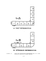
MULTIPLE VOLUME SOURCES . . . . . . . . . . . . . . 1-78
1-9
REPRESENTATION OF AN IRREGULARLY SHAPED AREA SOURCE
BY 4 RECTANGULAR AREA SOURCES . . . . . . . . . . .
1-79
1-10 EFFECTIVE AREA AND ALONGWIND LENGTH FOR AN OPEN PIT
SOURCE . . . . . . . . . . . . . . . . . . . . . . .
1-80
1-11 WET SCAVENGING RATE COEFFICIENT AS A FUNCTION OF PARTICLE
SIZE (JINDAL & HEINOLD, 1991) . . . . . . . . . . . 1-81
vii
TABLES
Page
Table
1-1
PARAMETERS USED TO CALCULATE PASQUILL-GIFFORD Fy . .
1-16
1-2
PARAMETERS USED TO CALCULATE PASQUILL-GIFFORD Fz . .
1-17
1-3
BRIGGS FORMULAS USED TO CALCULATE McELROY-POOLER Fy
1-19
1-4
BRIGGS FORMULAS USED TO CALCULATE McELROY-POOLER Fz
1-19
1-5
COEFFICIENTS USED TO CALCULATE LATERAL VIRTUAL
DISTANCES FOR PASQUILL-GIFFORD DISPERSION RATES
. .
1-21
SUMMARY OF SUGGESTED PROCEDURES FOR ESTIMATING
INITIAL LATERAL DIMENSIONS Fyo AND INITIAL VERTICAL
DIMENSIONS Fzo FOR VOLUME AND LINE SOURCES . . . . .
1-46
1-6
viii
SYMBOLS
Definition
Symbol
A
Linear decay term for vertical dispersion in
Schulman-Scire downwash (dimensionless)
Ae
Effective area for open pit emissions (dimensionless)
D
Exponential decay term for Gaussian plume equation
(dimensionless)
DB
Brownian diffusivity (cm/s)
Dr
Relative pit depth (dimensionless)
de
Effective pit depth (m)
dp
Particle diameter for particulate emissions (µm)
ds
Stack inside diameter (m)
Fb
Buoyancy flux parameter (m4/s3)
Fd
Dry deposition flux (g/m2)
Fm
Momentum flux parameter (m4/s2)
FQ
Plume depletion factor for dry deposition
(dimensionless)
FT
Terrain adjustment factor (dimensionless)
Fw
Wet deposition flux (g/m2)
f
Frequency of occurrence of a wind speed and stability
category combination (dimensionless)
g
Acceleration due to gravity (9.80616 m/s2)
hb
Building height (m)
he
Plume (or effective stack) height (m)
hs
Physical stack height (m)
hter
Height of terrain above stack base (m)
hs´
Release height modified for stack-tip downwash (m)
ix
hw
Crosswind projected width of building adjacent to a
stack (m)
k
von Karman constant (= 0.4)
L
Monin-Obukhov length (m)
Ly
Initial plume length for Schulman-Scire downwash
sources with enhanced lateral plume spread (m)
Lb
Lesser of the building height and crosswind projected
building width (m)
R
Alongwind length of open pit source (m)
P(x,y) Profile adjustment factor (dimensionless)
p
Wind speed power law profile exponent (dimensionless)
QA
Area Source pollutant emission rate (g/s)
Qe
Effective emission rate for effective area source for
an open pit source (g/s)
Qi
Adjusted emission rate for particle size category for
open pit emissions (g/s)
Qs
Pollutant emission rate (g/s)
QJ
Total amount of pollutant emitted during time period J
(g)
R
Precipitation rate (mm/hr)
Ro
Initial plume radius for Schulman-Scire downwash
sources (m)
R(z,zd)
Atmospheric resistance to vertical transport (s/cm)
r
Radial distance range in a polar receptor network (m)
ra
Atmospheric resistance (s/cm)
rd
Deposition layer resistance (s/cm)
s
Stability parameter = g
S
Smoothing term for smoothing across adjacent sectors in
the Long Term model (dimensionless)
Mθ/Mz
Ta
x
SCF
Splip correction factor (dimensionless)
Sc
Schmidt number = L/DB (dimensionless)
St
Stokes number =
Ta
Ambient temperature (K)
Ts
Stack gas exit temperature (K)
uref
( v g /g)
2
(u( /L) (dimensionless)
Wind speed measured at reference anemometer height
(m/s)
us
Wind speed adjusted to release height (m/s)
u*
Surface friction velocity (m/s)
V
Vertical term of the Gaussian plume equation
(dimensionless)
Vd
Vertical term with dry deposition of the Gaussian plume
equation (dimensionless)
vd
Particle deposition velocity (cm/s)
vg
Gravitational settling velocity for particles (cm/s)
vs
Stack gas exit velocity (m/s)
X
X-coordinate in a Cartesian grid receptor network (m)
xo
Length of side of square area source (m)
Y
Y-coordinate in a Cartesian grid receptor network (m)
2
Direction in a polar receptor network (degrees)
x
Downwind distance from source to receptor (m)
xy
Lateral virtual point source distance (m)
xz
Vertical virtual point source distance (m)
xf
Downwind distance to final plume rise (m)
x*
Downwind distance at which turbulence dominates
entrainment (m)
y
Crosswind distance from source to receptor (m)
z
Receptor/terrain height above mean sea level (m)
xi
zd
Dry deposition reference height (m)
zr
Receptor height above ground level (i.e. flagpole) (m)
zref
Reference height for wind speed power law (m)
zs
Stack base elevation above mean sea level (m)
zi
Mixing height (m)
z0
Surface roughness height (m)
$
Entrainment coefficient used in buoyant rise for
Schulman-Scire downwash sources = 0.6
$j
Jet entrainment coefficient used in gradual momentum
1 us
plume rise calculations ' %
3 vs
)h
Plume rise (m)
M2/Mz
Potential temperature gradient with height (K/m)
gi
Escape fraction of particle size category for open pit
emissions (dimensionless)
7
Precipitation scavenging ratio (s-1)
8
Precipitation rate coefficient (s-mm/hr)-1
B
pi = 3.14159
R
Decay coefficient = 0.693/T1/2 (s-1)
RH
Stability adjustment factor (dimensionless)
N
Fraction of mass in a particular settling velocity
category for particulates (dimensionless)
D
Particle density (g/cm3)
DAIR
Density of air (g/cm3)
Fy
Horizontal (lateral) dispersion parameter (m)
Fyo
Initial horizontal dispersion parameter for virtual
point source (m)
Fye
Effective lateral dispersion parameter including
effects of buoyancy-induced dispersion (m)
xii
Fz
Vertical dispersion parameter (m)
Fzo
Initial vertical dispersion parameter for virtual point
source (m)
Fze
Effective vertical dispersion parameter including
effects of buoyancy-induced dispersion (m)
L
Viscosity of air • 0.15 cm2/s
µ
Absolute viscosity of air • 1.81 x 10-4 g/cm/s
P
Concentration (µg/m3)
Pd
Concentration with dry deposition effects (µg/m3)
xiii
1.0 THE ISC SHORT-TERM DISPERSION MODEL EQUATIONS
The Industrial Source Complex (ISC) Short Term model
provides options to model emissions from a wide range of
sources that might be present at a typical industrial source
complex. The basis of the model is the straight-line,
steady-state Gaussian plume equation, which is used with some
modifications to model simple point source emissions from
stacks, emissions from stacks that experience the effects of
aerodynamic downwash due to nearby buildings, isolated vents,
multiple vents, storage piles, conveyor belts, and the like.
Emission sources are categorized into four basic types of
sources, i.e., point sources, volume sources, area sources, and
open pit sources. The volume source option and the area source
option may also be used to simulate line sources. The
algorithms used to model each of these source types are
described in detail in the following sections. The point
source algorithms are described in Section 1.1. The volume,
area and open pit source model algorithms are described in
Section 1.2. Section 1.3 gives the optional algorithms for
calculating dry deposition for point, volume, area and open pit
sources, and Section 1.4 describes the optional algorithms for
calculating wet deposition. Sections 1.1 through 1.4 describe
calculations for simple terrain (defined as terrain elevations
below the release height). The modifications to these
calculations to account for complex terrain are described in
Section 1.5, and the treatment of intermediate terrain is
discussed in Section 1.6.
The ISC Short Term model accepts hourly meteorological
data records to define the conditions for plume rise,
transport, diffusion, and deposition. The model estimates the
concentration or deposition value for each source and receptor
combination for each hour of input meteorology, and calculates
user-selected short-term averages. For deposition values,
either the dry deposition flux, the wet deposition flux, or the
total deposition flux may be estimated. The total deposition
1-1
flux is simply the sum of the dry and wet deposition fluxes at
a particular receptor location. The user also has the option
of selecting averages for the entire period of input
meteorology.
1.1 POINT SOURCE EMISSIONS
The ISC Short Term model uses a steady-state Gaussian
plume equation to model emissions from point sources, such as
stacks and isolated vents. This section describes the Gaussian
point source model, including the basic Gaussian equation, the
plume rise formulas, and the formulas used for determining
dispersion parameters.
1.1.1 The Gaussian Equation
The ISC short term model for stacks uses the steady-state
Gaussian plume equation for a continuous elevated source. For
each source and each hour, the origin of the source's
coordinate system is placed at the ground surface at the base
of the stack. The x axis is positive in the downwind
direction, the y axis is crosswind (normal) to the x axis and
the z axis extends vertically. The fixed receptor locations
are converted to each source's coordinate system for each
hourly concentration calculation. The calculation of the
downwind and crosswind distances is described in Section 1.1.2.
The hourly concentrations calculated for each source at each
receptor are summed to obtain the total concentration produced
at each receptor by the combined source emissions.
For a steady-state Gaussian plume, the hourly
concentration at downwind distance x (meters) and crosswind
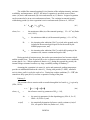
distance y (meters) is given by:
P '
QKVD
y
exp &0.5
2 B us Fy Fz
Fy
2
where:
1-2
(1-1)
Q
=
pollutant emission rate (mass per unit time)
K
=
a scaling coefficient to convert calculated
concentrations to desired units (default value of
1 x 106 for Q in g/s and concentration in µg/m3)
V
=
vertical term (See Section 1.1.6)
D
=
decay term (See Section 1.1.7)
Fy,Fz
=
standard deviation of lateral and vertical
concentration distribution (m) (See Section
1.1.5)
us
=
mean wind speed (m/s) at release height (See
Section 1.1.3)
Equation (1-1) includes a Vertical Term (V), a Decay Term
(D), and dispersion parameters (Fy and Fz) as discussed below.
It should be noted that the Vertical Term includes the effects
of source elevation, receptor elevation, plume rise, limited
mixing in the vertical, and the gravitational settling and dry
deposition of particulates (with diameters greater than about
0.1 microns).
1.1.2 Downwind and Crosswind Distances
The ISC model uses either a polar or a Cartesian receptor
network as specified by the user. The model allows for the use
of both types of receptors and for multiple networks in a
single run. All receptor points are converted to Cartesian
(X,Y) coordinates prior to performing the dispersion
calculations. In the polar coordinate system, the radial
coordinate of the point (r, 2) is measured from the
user-specified origin and the angular coordinate 2 is measured
clockwise from the north. In the Cartesian coordinate system,
the X axis is positive to the east of the user-specified origin
and the Y axis is positive to the north. For either type of
receptor network, the user must define the location of each
source with respect to the origin of the grid using Cartesian
coordinates. In the polar coordinate system, assuming the
1-3
origin is at X = Xo, Y = Yo, the X and Y coordinates of a
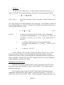
receptor at the point (r, 2) are given by:
X( R )
' r sin2 & Xo
(1-2)
Y( R )
' rcos2 & Y o
(1-3)
If the X and Y coordinates of the source are X(S) and Y(S), the
downwind distance x to the receptor, along the direction of
plume travel, is given by:
' &(X(R) & X(S))sin(WD) & (Y(R) & Y(S))cos(WD
(1-4)
where WD is the direction from which the wind is blowing. The
downwind distance is used in calculating the distance-dependent
plume rise (see Section 1.1.4) and the dispersion parameters
(see Section 1.1.5). If any receptor is located within 1 meter
of a point source or within 1 meter of the effective radius of
a volume source, a warning message is printed and no
concentrations are calculated for the source-receptor
combination. The crosswind distance y to the receptor from the
plume centerline is given by:
y ' (X(R) & X(S))cos(WD) & (Y(R) & Y(S))sin(WD)
(1-5)
The crosswind distance is used in Equation (1-1).
1.1.3 Wind Speed Profile
The wind power law is used to adjust the observed wind
speed, uref, from a reference measurement height, zref, to the
stack or release height, hs. The stack height wind speed, us,
is used in the Gaussian plume equation (Equation 1-1), and in
the plume rise formulas described in Section 1.1.4. The power
law equation is of the form:
u s ' uref
hs
p
(1-6)
z ref
1-4
where p is the wind profile exponent. Values of p may be
provided by the user as a function of stability category and
wind speed class. Default values are as follows:
Stability Category
Rural Exponent
Urban Exponent
A
0.07
0.15
B
0.07
0.15
C
0.10
0.20
D
0.15
0.25
E
0.35
0.30
F
0.55
0.30
The stack height wind speed, us, is not allowed to be less
than 1.0 m/s.
1.1.4 Plume Rise Formulas
The plume height is used in the calculation of the
Vertical Term described in Section 1.1.6. The Briggs plume
rise equations are discussed below. The description follows
Appendix B of the Addendum to the MPTER User's Guide (Chico and
Catalano, 1986) for plumes unaffected by building wakes. The
distance dependent momentum plume rise equations, as described
in (Bowers, et al., 1979), are used to determine if the plume
is affected by the wake region for building downwash
calculations. These plume rise calculations for wake
determination are made assuming no stack-tip downwash for both
the Huber-Snyder and the Schulman-Scire methods. When the
model executes the building downwash methods of Schulman and
Scire, the reduced plume rise suggestions of Schulman and Scire
(1980) are used, as described in Section 1.1.4.11.
1-5
1.1.4.1 Stack-tip Downwash.
In order to consider stack-tip downwash, modification of
the physical stack height is performed following Briggs (1974,
p. 4). The modified physical stack height hs´ is found from:
h s´
' h s % 2ds
vs
& 1.5
us
for v s < 1.5u
(1-7)
or
for vs $ 1.5
hs ´ ' h s
where hs is physical stack height (m), vs is stack gas exit
velocity (m/s), and ds is inside stack top diameter (m). This
hs´ is used throughout the remainder of the plume height
computation. If stack tip downwash is not considered, hs´ = hs
in the following equations.
1.1.4.2 Buoyancy and Momentum Fluxes.
For most plume rise situations, the value of the Briggs
buoyancy flux parameter, Fb (m4/s3), is needed. The following
equation is equivalent to Equation (12), (Briggs, 1975, p. 63):
Fb
)T
4Ts
2
' gv s ds
(1-8)
where )T = Ts - Ta, Ts is stack gas temperature (K), and Ta is
ambient air temperature (K).
For determining plume rise due to the momentum of the
plume, the momentum flux parameter, Fm (m4/s2), is calculated
based on the following formula:
Fm
2
2
' vs ds
Ta
(1-9)
4T s
1-6
1.1.4.3 Unstable or Neutral - Crossover Between Momentum
and Buoyancy.
For cases with stack gas temperature greater than or equal
to ambient temperature, it must be determined whether the plume
rise is dominated by momentum or buoyancy. The crossover
temperature difference, ()T)c, is determined by setting Briggs'
(1969, p. 59) Equation 5.2 equal to the combination of Briggs'
(1971, p. 1031) Equations 6 and 7, and solving for )T, as
follows:
for Fb < 55,
1/ 3
(
)T )c ' 0.0297 T s
vs
2/ 3
(1-10)
ds
and for Fb $ 55,
2/ 3
(
)T )c ' 0.00575 T s
vs
1/ 3
(1-11)
ds
If the difference between stack gas and ambient temperature,
)T, exceeds or equals ()T)c, plume rise is assumed to be
buoyancy dominated, otherwise plume rise is assumed to be
momentum dominated.
1.1.4.4 Unstable or Neutral - Buoyancy Rise.
For situations where )T exceeds ()T)c as determined above,
buoyancy is assumed to dominate. The distance to final rise,
xf, is determined from the equivalent of Equation (7), (Briggs,
1971, p. 1031), and the distance to final rise is assumed to be
3.5x*, where x* is the distance at which atmospheric turbulence
begins to dominate entrainment. The value of xf is calculated
as follows:
for Fb < 55:
x f
5/ 8
' 49Fb
(1-12)
1-7
and for Fb $ 55:
x f
2/ 5
' 119Fb
(1-13)
The final effective plume height, he (m), is determined
from the equivalent of the combination of Equations (6) and (7)
(Briggs, 1971, p. 1031):
for Fb < 55:
3/ 4
' h s ´ % 21.425
h e
Fb
(1-14)
us
and for Fb $ 55:
3/ 5
h e
' h s ´ % 38.71
Fb
(1-15)
us
1.1.4.5 Unstable or Neutral - Momentum Rise.
For situations where the stack gas temperature is less
than or equal to the ambient air temperature, the assumption is
made that the plume rise is dominated by momentum. If )T is
less than ()T)c from Equation (1-10) or (1-11), the assumption
is also made that the plume rise is dominated by momentum. The
plume height is calculated from Equation (5.2) (Briggs, 1969,
p. 59):
h e
' hs ´ % 3d s
vs
(1-16)
us
Briggs (1969, p. 59) suggests that this equation is most
applicable when vs/us is greater than 4.
1.1.4.6 Stability Parameter.
For stable situations, the stability parameter, s, is
calculated from the Equation (Briggs, 1971, p. 1031):
1-8
M2/Mz
(1-17)
Ta
As a default approximation, for stability class E (or 5) M2/Mz
is taken as 0.020 K/m, and for class F (or 6), M2/Mz is taken
as 0.035 K/m.
s
' g
1.1.4.7 Stable - Crossover Between Momentum and Buoyancy.
For cases with stack gas temperature greater than or equal
to ambient temperature, it must be determined whether the plume
rise is dominated by momentum or buoyancy. The crossover
temperature difference, ()T)c , is determined by setting
Briggs' (1975, p. 96) Equation 59 equal to Briggs' (1969, p.
59) Equation 4.28, and solving for )T, as follows:
(
)T) c ' 0.019582 Ts v s s
(1-18)
If the difference between stack gas and ambient temperature,
)T, exceeds or equals ()T)c, plume rise is assumed to be
buoyancy dominated, otherwise plume rise is assumed to be
momentum dominated.
1.1.4.8 Stable - Buoyancy Rise.
For situations where )T exceeds ()T)c as determined above,
buoyancy is assumed to dominate. The distance to final rise,
xf, is determined by the equivalent of a combination of
Equations (48) and (59) in Briggs, (1975), p. 96:
x f ' 2.0715
us
(1-19)
s
The plume height, he, is determined by the equivalent of
Equation (59) (Briggs, 1975, p. 96):
h e ' hs ´ % 2.6
Fb
1/ 3
(1-20)
us s
1-9
1.1.4.9 Stable - Momentum Rise.
Where the stack gas temperature is less than or equal to
the ambient air temperature, the assumption is made that the
plume rise is dominated by momentum. If )T is less than ()T)c
as determined by Equation (1-18), the assumption is also made
that the plume rise is dominated by momentum. The plume height
is calculated from Equation 4.28 of Briggs ((1969), p. 59):
h e
1/ 3
Fm
' h s ´ % 1.5
(1-21)
us s
The equation for unstable-neutral momentum rise (1-16) is also
evaluated. The lower result of these two equations is used as
the resulting plume height, since stable plume rise should not
exceed unstable-neutral plume rise.
1.1.4.10 All Conditions - Distance Less Than Distance to
Final Rise.
Where gradual rise is to be estimated for unstable,
neutral, or stable conditions, if the distance downwind from
source to receptor, x, is less than the distance to final rise,
the equivalent of Equation 2 of Briggs ((1972), p. 1030) is
used to determine plume height:
1/ 3
h e
' h s ´ % 1.60
Fb
x 2/ 3
(1-22)
us
This height will be used only for buoyancy dominated
conditions; should it exceed the final rise for the appropriate
condition, the final rise is substituted instead.
For momentum dominated conditions, the following equations
(Bowers, et al, 1979) are used to calculate a distance
dependent momentum plume rise:
a) unstable conditions:
1-10
h e
' hs ´ %
3F m x
2
$j
1/ 3
(1-23)
2
us
where x is the downwind distance (meters), with a maximum value
defined by xmax as follows:
x max
'
4ds (v s % 3us )2
for Fb ' 0
vs u s
5/ 8
for 0 < F b # 55m4 /s 3
' 49F b
2/ 5
(1-24)
for F b > 55m4 /s 3
' 119F b
b) stable conditions:
h e
' h s ´ % 3 Fm
sin(x s/u s )
1/ 3
2
$j u s s
(1-25)
where x is the downwind distance (meters), with a maximum value
defined by xmax as follows:
x max
' 0.5
Bus
(1-26)
s
The jet entrainment coefficient, $j, is given by,
$j '
u
1
% s
3
vs
(1-27)
As with the buoyant gradual rise, if the distance-dependent
momentum rise exceeds the final rise for the appropriate
condition, then the final rise is substituted instead.
1.1.4.10.1 Calculating the plume height for wake effects
determination.
The building downwash algorithms in the ISC models always
require the calculation of a distance dependent momentum plume
rise. When building downwash is being simulated, the equations
1-11
described above are used to calculate a distance dependent
momentum plume rise at a distance of two building heights
downwind from the leeward edge of the building. However,
stack-tip downwash is not used when performing this calculation
(i.e. hs´ = hs). This wake plume height is compared to the
wake height based on the good engineering practice (GEP)
formula to determine whether the building wake effects apply to
the plume for that hour.
The procedures used to account for the effects of building
downwash are discussed more fully in Section 1.1.5.3. The
plume rise calculations used with the Schulman-Scire algorithm
are discussed in Section 1.1.4.11.
1.1.4.11 Plume Rise When Schulman and Scire Building
Downwash is Selected.
The Schulman-Scire downwash algorithms are used by the ISC
models when the stack height is less than the building height
plus one half of the lesser of the building height or width.
When these criteria are met, the ISC models estimate plume rise
during building downwash conditions following the suggestion of
Scire and Schulman (1980). The plume rise during building
downwash conditions is reduced due to the initial dilution of
the plume with ambient air.
The plume rise is estimated as follows. The initial
dimensions of the downwashed plume are approximated by a line
source of length Ly and depth 2Ro where:
Ro
'
2AFz
x ' 3LB
(1-28)
Ly ' 2B (Fy & Fz )
x ' 3L B, Fy $ Fz
(1-29a)
Ly ' 0
x ' 3L B, Fy < Fz
(1-29b)
1-12
LB equals the minimum of hb and hw, where hb is the building
height and hw the projected (crosswind) building width. A is a
linear decay factor and is discussed in more detail in Section
1.1.5.3.2. If there is no enhancement of Fy or if the enhanced
Fy is less than the enhanced Fz, the initial plume will be
represented by a circle of radius Ro.
The
2 factor converts
the Gaussian Fz to an equivalent uniform circular distribution
2B converts Fy to an equivalent uniform rectangular
and
Both Fy and Fz are evaluated at x = 3LB, and are
taken as the larger of the building enhanced sigmas and the
sigmas obtained from the curves (see Section 1.1.5.3). The
value of Fz used in the calculation of Ly also includes the
linear decay term, A.
distribution.
The rise of a downwashed finite line source was solved in
the BLP model (Scire and Schulman, 1980). The neutral
distance-dependent rise (Z) is given by:
3
Z
%
3Ly
B$
%
3R o
Z
$
2
%
2
6R o Ly
3R o
%
B$2
Z '
$2
3
(1-30)
2
The stable distance-dependent rise is calculated by:
Z
3
3Ly
%
B$
%
3R o
Z
$
2
6R o Ly
%
B$2
2
%
3R o
$2
Z '
3F b x 2
(1-31a)
3
2$2 u s
with a maximum stable buoyant rise given by:
Z
3
%
3Ly
B$
%
3R o
$
Z
2
%
6R o Ly
B$
2
2
%
3R o
$
2
Z '
where:
Fb
= buoyancy flux term (Equation 1-8) (m4/s3)
1-13
(1-31b)
Fm
= momentum flux term (Equation 1-9) (m4/s2)
x
= downwind distance (m)
us
= wind speed at release height (m/s)
vs
= stack exit velocity (m/s)
ds
= stack diameter (m)
$
= entrainment coefficient (=0.6)
$j
= jet entrainment coefficient
s
= stability parameter
' g
'
1 us
%
3 vs
M2/Mz
Ta
The larger of momentum and buoyant rise, determined separately
by alternately setting Fb or Fm = 0 and solving for Z, is
selected for plume height calculations for Schulman-Scire
downwash. In the ISC models, Z is determined by solving the
cubic equation using Newton's method.
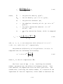
1.1.5 The Dispersion Parameters
1.1.5.1 Point Source Dispersion Parameters.
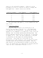
Equations that approximately fit the Pasquill-Gifford
curves (Turner, 1970) are used to calculate Fy and Fz (in
meters) for the rural mode. The equations used to calculate Fy
are of the form:
Fy ' 465.11628(x)tan(TH)
(1-32)
TH ' 0.017453293[c & d ln(x)]
(1-33)
where:
1-14
In Equations (1-32) and (1-33) the downwind distance x is in
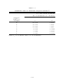
kilometers, and the coefficients c and d are listed in Table
1-1. The equation used to calculate Fz is of the form:
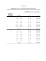
Fz ' ax b
(1-34)
where the downwind distance x is in kilometers and Fz is in
meters. The coefficients a and b are given in Table 1-2.
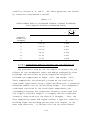
Tables 1-3 and 1-4 show the equations used to determine Fy
and Fz for the urban option. These expressions were determined
by Briggs as reported by Gifford (1976) and represent a best
fit to urban vertical diffusion data reported by McElroy and
Pooler (1968). While the Briggs functions are assumed to be
valid for downwind distances less than 100m, the user is
cautioned that concentrations at receptors less than 100m from
a source may be suspect.
1-15
TABLE 1-1
PARAMETERS USED TO CALCULATE PASQUILL-GIFFORD Fy
Fy = 465.11628 (x)tan(TH)
TH = 0.017453293 [c - d ln(x)]
Pasquill
Stability
Category
c
d
A
24.1670
2.5334
B
18.3330
1.8096
C
12.5000
1.0857
D
8.3330
0.72382
E
6.2500
0.54287
F
4.1667
0.36191
where Fy is in meters and x is in kilometers
1-16
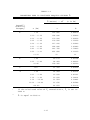
TABLE 1-2
PARAMETERS USED TO CALCULATE PASQUILL-GIFFORD Fz
Fz(meters) = axb
Pasquill
Stability
Category
x (km)
a
(x in km)
b
A*
<.10
0.10 - 0.15
0.16 - 0.20
0.21 - 0.25
0.26 - 0.30
0.31 - 0.40
0.41 - 0.50
0.51 - 3.11
>3.11
122.800
158.080
170.220
179.520
217.410
258.890
346.750
453.850
**
0.94470
1.05420
1.09320
1.12620
1.26440
1.40940
1.72830
2.11660
**
B*
<.20
0.21 - 0.40
>0.40
90.673
98.483
109.300
0.93198
0.98332
1.09710
C*
All
61.141
0.91465
D
<.30
0.31 - 1.00
1.01 - 3.00
3.01 - 10.00
10.01 - 30.00
>30.00
34.459
32.093
32.093
33.504
36.650
44.053
0.86974
0.81066
0.64403
0.60486
0.56589
0.51179
*
If the calculated value of Fz exceed 5000 m, Fz is set to
5000 m.
**
Fz is equal to 5000 m.
1-17
TABLE 1-2
(CONTINUED)
PARAMETERS USED TO CALCULATE PASQUILL-GIFFORD Fz
Fz(meters) = axb
Pasquill
Stability
Category
x (km)
a
(x in km)
b
E
<.10
0.10 - 0.30
0.31 - 1.00
1.01 - 2.00
2.01 - 4.00
4.01 - 10.00
10.01 - 20.00
20.01 - 40.00
>40.00
24.260
23.331
21.628
21.628
22.534
24.703
26.970
35.420
47.618
0.83660
0.81956
0.75660
0.63077
0.57154
0.50527
0.46713
0.37615
0.29592
F
<.20
0.21 - 0.70
0.71 - 1.00
1.01 - 2.00
2.01 - 3.00
3.01 - 7.00
7.01 - 15.00
15.01 - 30.00
30.01 - 60.00
>60.00
15.209
14.457
13.953
13.953
14.823
16.187
17.836
22.651
27.074
34.219
0.81558
0.78407
0.68465
0.63227
0.54503
0.46490
0.41507
0.32681
0.27436
0.21716
1-18
TABLE 1-3
BRIGGS FORMULAS USED TO CALCULATE McELROY-POOLER Fy
Pasquill
Stability
Category
*
Fy(meters)*
A
0.32 x (1.0 + 0.0004 x)-1/2
B
0.32 x (1.0 + 0.0004 x)-1/2
C
0.22 x (1.0 + 0.0004 x)-1/2
D
0.16 x (1.0 + 0.0004 x)-1/2
E
0.11 x (1.0 + 0.0004 x)-1/2
F
0.11 x (1.0 + 0.0004 x)-1/2
Where x is in meters
TABLE 1-4
BRIGGS FORMULAS USED TO CALCULATE McELROY-POOLER Fz
Pasquill
Stability
Category
*
Fz(meters)*
A
0.24 x (1.0 + 0.001 x)1/2
B
0.24 x (1.0 + 0.001 x)1/2
C
0.20 x
D
0.14 x (1.0 + 0.0003 x)-1/2
E
0.08 x (1.0 + 0.0015 x)-1/2
F
0.08 x (1.0 + 0.0015 x)-1/2
Where x is in meters.
1-19
1.1.5.2 Lateral and Vertical Virtual Distances.
The equations in Tables 1-1 through 1-4 define the
dispersion parameters for an ideal point source. However,
volume sources have initial lateral and vertical dimensions.
Also, as discussed below, building wake effects can enhance the
initial growth of stack plumes. In these cases, lateral (xy)
and vertical (xz) virtual distances are added by the ISC models
to the actual downwind distance x for the Fy and Fz
calculations. The lateral virtual distance in kilometers for
the rural mode is given by:
x y
'
Fyo
1/ q
(1-35)
p
where the stability-dependent coefficients p and q are given in
Table 1-5 and Fyo is the standard deviation in meters of the
lateral concentration distribution at the source. Similarly,
the vertical virtual distance in kilometers for the rural mode
is given by:
x z
'
Fzo
1/ b
(1-36)
a
where the coefficients a and b are obtained form Table 1-2 and
Fzo is the standard deviation in meters of the vertical
concentration distribution at the source. It is important to
note that the ISC model programs check to ensure that the xz
used to calculate Fz at (x + xz) in the rural mode is the xz
calculated using the coefficients a and b that correspond to
the distance category specified by the quantity (x + xz).
To determine virtual distances for the urban mode, the
functions displayed in Tables 1-3 and 1-4 are solved for x.
The solutions are quadratic formulas for the lateral virtual
distances; and for vertical virtual distances the solutions are
cubic equations for stability classes A and B, a linear
equation for stability class C, and quadratic equations for
1-20
stability classes D, E, and F. The cubic equations are solved
by iteration using Newton's method.
TABLE 1-5
COEFFICIENTS USED TO CALCULATE LATERAL VIRTUAL DISTANCES
FOR PASQUILL-GIFFORD DISPERSION RATES
x y
'
Pasquill
Stability
Category
p
q
A
209.14
0.890
B
154.46
0.902
C
103.26
0.917
D
68.26
0.919
E
51.06
0.921
F
33.92
0.919
Fyo
1/ q
p
1.1.5.3 Procedures Used to Account for the Effects of
Building Wakes on Effluent Dispersion.
The procedures used by the ISC models to account for the
effects of the aerodynamic wakes and eddies produced by plant
buildings and structures on plume dispersion originally
followed the suggestions of Huber (1977) and Snyder (1976).
Their suggestions are principally based on the results of
wind-tunnel experiments using a model building with a crosswind
dimension double that of the building height. The atmospheric
turbulence simulated in the wind-tunnel experiments was
intermediate between the turbulence intensity associated with
the slightly unstable Pasquill C category and the turbulence
intensity associated with the neutral D category. Thus, the
data reported by Huber and Snyder reflect a specific stability,
building shape and building orientation with respect to the
mean wind direction. It follows that the ISC wake-effects
1-21
evaluation procedures may not be strictly applicable to all
situations. The ISC models also provide for the revised
treatment of building wake effects for certain sources, which
uses modified plume rise algorithms, following the suggestions
of Schulman and Hanna (1986). This treatment is largely based
on the work of Scire and Schulman (1980). When the stack
height is less than the building height plus half the lesser of
the building height or width, the methods of Schulman and Scire
are followed. Otherwise, the methods of Huber and Snyder are
followed. In the ISC models, direction-specific building
dimensions may be used with either the Huber-Snyder or
Schulman-Scire downwash algorithms.
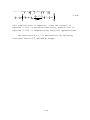
The wake-effects evaluation procedures may be applied by
the user to any stack on or adjacent to a building. For
regulatory application, a building is considered sufficiently
close to a stack to cause wake effects when the distance
between the stack and the nearest part of the building is less
than or equal to five times the lesser of the height or the
projected width of the building. For downwash analyses with
direction-specific building dimensions, wake effects are
assumed to occur if the stack is within a rectangle composed of
two lines perpendicular to the wind direction, one at 5Lb
downwind of the building and the other at 2Lb upwind of the
building, and by two lines parallel to the wind direction, each
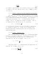
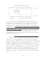
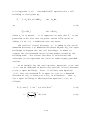
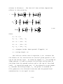
at 0.5Lb away from each side of the building, as shown below:
1-22
Wind direction )))))))))))))>
+)))))))))))))))))))))))))))))))))))))))))),
*
*
*
+)), ) ) ) ) ) ) ) ) ) ) ) ) *
+))- .)),
*
*
*Building*
*
*
*
*
*
*
.))))), *
*
*
* *
*
*
.))- ) ) ) ) ) ) ) ) ) ) ) *
*
*
*
.))))))))))))))))))))))))))))))))))))))))))*<))2Lb))>*
))
))
1/2 Lb
))
))
1/2 Lb
*<)))))))))5Lb)))))))))>*
Lb is the lesser of the height and projected width of the
building for the particular direction sector. For additional
guidance on determining whether a more complex building
configuration is likely to cause wake effects, the reader is
referred to the Guideline for Determination of Good Engineering
Practice Stack Height (Technical Support Document for the Stack
Height Regulations) - Revised (EPA, 1985). In the following
sections, the Huber and Snyder building downwash method is
described followed by a description of the Schulman and Scire
building downwash method.
1.1.5.3.1 Huber and Snyder building downwash procedures.
The first step in the wake-effects evaluation procedures
used by the ISC model programs is to calculate the gradual
plume rise due to momentum alone at a distance of two building
heights using Equation (1-23) or Equation (1-25). If the plume
height, he, given by the sum of the stack height (with no
stack-tip downwash adjustment) and the momentum rise is greater
than either 2.5 building heights (2.5 hb) or the sum of the
building height and 1.5 times the building width (hb + 1.5 hw),
the plume is assumed to be unaffected by the building wake.
Otherwise the plume is assumed to be affected by the building
wake.
1-23
The ISC model programs account for the effects of building
wakes by modifying both Fy and Fz for plumes with plume height
to building height ratios less than or equal to 1.2 and by
modifying only Fz for plumes from stacks with plume height to
building height ratios greater than 1.2 (but less than 2.5).
The plume height used in the plume height to stack height
ratios is the same plume height used to determine if the plume
is affected by the building wake. The ISC models define
buildings as squat (hw $ hb) or tall (hw < hb). The ISC models
include a general procedure for modifying Fz and Fy at
distances greater than or equal to 3hb for squat buildings or
3hw for tall buildings. The air flow in the building cavity
region is both highly turbulent and generally recirculating.
The ISC models are not appropriate for estimating
concentrations within such regions. The ISC assumption that
this recirculating cavity region extends to a downwind distance
of 3hb for a squat building or 3hw for a tall building is most
appropriate for a building whose width is not much greater than
its height. The ISC user is cautioned that, for other types of
buildings, receptors located at downwind distances of 3hb
(squat buildings) or 3hw (tall buildings) may be within the
recirculating region.
The modified Fz equation for a squat building is given by:
Fz ´ ' 0.7hb % 0.067(x&3h b )
for 3hb # x
(1-37)
or
' Fz {x % xz }
for x $ 10h b
where the building height hb is in meters. For a tall
building, Huber (1977) suggests that the width scale hw replace
1-24
hb in Equation (1-37). The modified Fz equation for a tall
building is then given by:
Fz ´ ' 0.7hw % 0.067(x&3h w)
for 3hw # x
(1-38)
or
' Fz {x % xz }
for x $ 10h w
where hw is in meters. It is important to note that Fz´ is not
permitted to be less than the point source value given in
Tables 1-2 or 1-4, a condition that may occur.
The vertical virtual distance, xz, is added to the actual
downwind distance x at downwind distances beyond 10hb for squat
buildings or beyond 10hw for tall buildings, in order to
account for the enhanced initial plume growth caused by the
building wake. The virtual distance is calculated from
solutions to the equations for rural or urban sigmas provided
earlier.
As an example for the rural options, Equations (1-34) and
(1-37) can be combined to derive the vertical virtual distance
xz for a squat building. First, it follows from Equation
(1-37) that the enhanced Fz is equal to 1.2hb at a downwind
distance of 10hb in meters or 0.01hb in kilometers. Thus, xz
for a squat building is obtained from Equation (1-34) as
follows:
Fz {0.01h b } ' 1.2hb ' a(0.01h b % xz ) b
x z
'
1.2hb
a
(1-39)
1/ b
& 0.01hb
1-25
(1-40)
where the stability-dependent constants a and b are given in
Table 1-2. Similarly, the vertical virtual distance for tall
buildings is given by:
x z
'
1.2hw
a
1/ b
& 0.01hw
(1-41)
For the urban option, xz is calculated from solutions to the
equations in Table 1-4 for Fz = 1.2hb or Fz = 1.2 hw for tall or
squat buildings, respectively.
For a squat building with a building width to building
height ratio (hw/hb) less than or equal to 5, the modified Fy
equation is given by:
Fy ´ ' 0.35hw % 0.067(x&3h b )
for 3hb # x
(1-42)
or
' Fy {x % xy }
for x $ 10h b
The lateral virtual distance is then calculated for this value
of Fy.
For a building that is much wider than it is tall (hw/hb
greater than 5), the presently available data are insufficient
to provide general equations for Fy. For a stack located
toward the center of such a building (i.e., away form either
end), only the height scale is considered to be significant.
1-26
The modified Fy equation for a very squat building is then
given by:
Fy ´ ' 0.35hb % 0.067(x&3h b )
for 3hb # x
(1-43)
or
' Fy {x % xy }
for x $ 10h b
For hw/hb greater than 5, and a stack located laterally
within about 2.5 hb of the end of the building, lateral plume
spread is affected by the flow around the end of the building.
With end effects, the enhancement in the initial lateral spread
is assumed not to exceed that given by Equation (1-42) with hw
replaced by 5 hb.
The modified Fy equation is given by:
Fy ´ ' 1.75hb % 0.067(x&3h b )
for 3hb # x
(1-44)
or
' Fy {x % xy }
for x $ 10h
The upper and lower bounds of the concentrations that can
be expected to occur near a building are determined
respectively using Equations (1-43) and (1-44). The user must
specify whether Equation (1-43) or Equation (1-44) is to be
used in the model calculations. In the absence of user
instructions, the ISC models use Equation (1-43) if the
building width to building height ratio hw/hb exceeds 5.
Although Equation (1-43) provides the highest
concentration estimates for squat buildings with building width
to building height ratios (hw/hb) greater than 5, the equation
is applicable only to a stack located near the center of the
building when the wind direction is perpendicular to the long
side of the building (i.e., when the air flow over the portion
1-27
of the building containing the source is two dimensional).
Thus, Equation (1-44) generally is more appropriate then
Equation (1-43). It is believed that Equations (1-43) and
(1-44) provide reasonable limits on the extent of the lateral
enhancement of dispersion and that these equations are adequate
until additional data are available to evaluate the flow near
very wide buildings.
The modified Fy equation for a tall building is given by:
Fy ´ ' 0.35hw % 0.067(x&3h w)
for 3hw # x
(1-45)
or
' Fy {x % xy }
for x $ 10h
The ISC models print a message and do not calculate
concentrations for any source-receptor combination where the
source-receptor separation is less than 1 meter, and also for
distances less than 3 hb for a squat building or 3 hw for a
tall building under building wake effects. It should be noted
that, for certain combinations of stability and building height
and/or width, the vertical and/or lateral plume dimensions
indicated for a point source by the dispersion curves at a
downwind distance of ten building heights or widths can exceed
the values given by Equation (1-37) or (1-38) and by Equation
(1-42) or (1-43). Consequently, the ISC models do not permit
the virtual distances xy and xz to be less than zero.
1.1.5.3.2 Schulman and Scire refined building downwash
procedures.
The procedures for treating building wake effects include
the use of the Schulman and Scire downwash method. The
building wake procedures only use the Schulman and Scire method
when the physical stack height is less than hb + 0.5 LB, where
hb is the building height and LB is the lesser of the building
1-28
height or width. In regulatory applications, the maximum
projected width is used. The features of the Schulman and
Scire method are: (1) reduced plume rise due to initial plume
dilution, (2) enhanced vertical plume spread as a linear
function of the effective plume height, and (3) specification
of building dimensions as a function of wind direction. The
reduced plume rise equations were previously described in
Section 1.1.4.11.
When the Schulman and Scire method is used, the ISC
dispersion models specify a linear decay factor, to be included
in the Fz's calculated using Equations (1-37) and (1-38), as
follows:
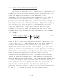
Fz ´´ ' AFz ´
(1-46)
where Fz´ is from either Equation (1-37) or (1-38) and A is the
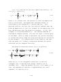
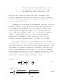
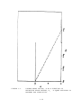
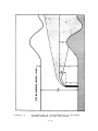
linear decay factor determined as follows:
if h e # hb
A ' 1
A '
hb & h e
2LB
A ' 0
% 1
if h b < he # h b % 2LB
(1-47)
if h e > hb % 2LB
where the plume height, he, is the height due to gradual
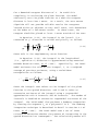
momentum rise at 2 hb used to check for wake effects. The
effect of the linear decay factor is illustrated in Figure 1-1.
For Schulman-Scire downwash cases, the linear decay term is
also used in calculating the vertical virtual distances with
Equations (1-40) to (1-41).
When the Schulman and Scire building downwash method is
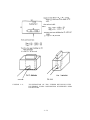
used the ISC models require direction specific building heights
and projected widths for the downwash calculations. The ISC
models also accept direction specific building dimensions for
Huber-Snyder downwash cases. The user inputs the building
height and projected widths of the building tier associated
1-29
with the greatest height of wake effects for each ten degrees
of wind direction. These building heights and projected widths
are the same as are used for GEP stack height calculations.
The user is referred to EPA (1986) for calculating the
appropriate building heights and projected widths for each
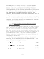
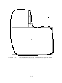
direction. Figure 1-2 shows an example of a two tiered
building with different tiers controlling the height that is
appropriate for use for different wind directions. For an east
or west wind the lower tier defines the appropriate height and
width, while for a north or south wind the upper tier defines
the appropriate values for height and width.
1.1.5.4 Procedures Used to Account for Buoyancy-Induced
Dispersion.
The method of Pasquill (1976) is used to account for the
initial dispersion of plumes caused by turbulent motion of the
plume and turbulent entrainment of ambient air. With this
method, the effective vertical dispersion Fze is calculated as
follows:
Fze '
2
Fz
%
)h
3.5
2
1/ 2
(1-48)
where Fz is the vertical dispersion due to ambient turbulence
and )h is the plume rise due to momentum and/or buoyancy. The
lateral plume spread is parameterized using a similar
expression:
Fye '
2
Fy
%
)h
3.5
2
1/ 2
(1-49)
where Fy is the lateral dispersion due to ambient turbulence.
It should be noted that )h is the distance-dependent plume
rise if the receptor is located between the source and the
distance to final rise, and final plume rise if the receptor is
located beyond the distance to final rise. Thus, if the user
1-30
elects to use final plume rise at all receptors the
distance-dependent plume rise is used in the calculation of
buoyancy-induced dispersion and the final plume rise is used in
the concentration equations. It should also be noted that
buoyancy-induced dispersion is not used when the Schulman-Scire
downwash option is in effect.
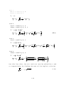
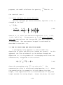
1.1.6 The Vertical Term
The Vertical Term (V), which is included in Equation
(1-1), accounts for the vertical distribution of the Gaussian
plume. It includes the effects of source elevation, receptor
elevation, plume rise (Section 1.1.4), limited mixing in the
vertical, and the gravitational settling and dry deposition of
particulates. In addition to the plume height, receptor height
and mixing height, the computation of the Vertical Term
requires the vertical dispersion parameter (Fz) described in
Section 1.1.5.
1.1.6.1 The Vertical Term Without Dry Deposition.
In general, the effects on ambient concentrations of
gravitational settling and dry deposition can be neglected for
gaseous pollutants and small particulates (less than about 0.1
1-31
microns in diameter). The Vertical Term without deposition
effects is then given by:
V
' exp &0.5
zr & h e
% exp &0.5
Fz
4
% j
2
exp &0.5
i '1
% exp &0.5
H2
% exp &0.5
Fz
H3
Fz
2
H1
2
Fz
2
z r % he
% exp &0.5
2
Fz
H4
2
(1-50)
Fz
where:
he = hs + )h
H1 = zr - (2izi - he)
H2 = zr + (2izi - he)
H3 = zr - (2izi + he)
H4 = zr + (2izi + he)
zr = receptor height above ground (flagpole) (m)
zi = mixing height (m)
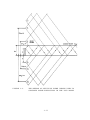
The infinite series term in Equation (1-50) accounts for
the effects of the restriction on vertical plume growth at the
top of the mixing layer. As shown by Figure 1-3, the method of
image sources is used to account for multiple reflections of
the plume from the ground surface and at the top of the mixed
layer. It should be noted that, if the effective stack height,
he, exceeds the mixing height, zi, the plume is assumed to
fully penetrate the elevated inversion and the ground-level
concentration is set equal to zero.
1-32
Equation (1-50) assumes that the mixing height in rural
and urban areas is known for all stability categories. As
explained below, the meteorological preprocessor program uses
mixing heights derived from twice-daily mixing heights
calculated using the Holzworth (1972) procedures. The ISC
models currently assume unlimited vertical mixing under stable
conditions, and therefore delete the infinite series term in
Equation (1-50) for the E and F stability categories.
The Vertical Term defined by Equation (1-50) changes the
form of the vertical concentration distribution from Gaussian
to rectangular (i.e., a uniform concentration within the
surface mixing layer) at long downwind distances.
Consequently, in order to reduce computational time without a
loss of accuracy, Equation (1-50) is changed to the form:
V
'
2B Fz
(1-51)
zi
at downwind distances where the Fz/zi ratio is greater than or
equal to 1.6.
The meteorological preprocessor program, RAMMET, used by
the ISC Short Term model uses an interpolation scheme to assign
hourly rural and urban mixing heights on the basis of the early
morning and afternoon mixing heights calculated using the
Holzworth (1972) procedures. The procedures used to
interpolate hourly mixing heights in urban and rural areas are
illustrated in Figure 1-4, where:
Hm{max}
Hm{min}
MN
SR
SS
=
=
=
=
=
maximum mixing height on a given day
minimum mixing height on a given day
midnight
sunrise
sunset
The interpolation procedures are functions of the stability
category for the hour before sunrise. If the hour before
sunrise is neutral, the mixing heights that apply are indicated
1-33
by the dashed lines labeled neutral in Figure 1-4. If the hour
before sunrise is stable, the mixing heights that apply are
indicated by the dashed lines labeled stable. It should be
pointed out that there is a discontinuity in the rural mixing
height at sunrise if the preceding hour is stable. As
explained above, because of uncertainties about the
applicability of Holzworth mixing heights during periods of E
and F stability, the ISC models ignore the interpolated mixing
heights for E and F stability, and treat such cases as having
unlimited vertical mixing.
1.1.6.2 The Vertical Term in Elevated Simple Terrain.
The ISC models make the following assumption about plume
behavior in elevated simple terrain (i.e., terrain that exceeds
the stack base elevation but is below the release height):
$
The plume axis remains at the plume stabilization
height above mean sea level as it passes over elevated
or depressed terrain.
$
The mixing height is terrain following.
$
The wind speed is a function of height above the
surface (see Equation (1-6)).
Thus, a modified plume stabilization height he´ is
substituted for the effective stack height he in the Vertical
Term given by Equation (1-50). For example, the effective
plume stabilization height at the point x, y is given by:
h e´
' h e % zs & z*( x, y)
(1-52)
where:
zs
z*(x,y)
= height above mean sea level of the base of the
stack (m)
= height above mean sea level of terrain at the
receptor location (x,y) (m)
1-34
It should also be noted that, as recommended by EPA, the ISC
models "truncate" terrain at stack height as follows: if the
terrain height z - zs exceeds the source release height, hs,
the elevation of the receptor is automatically "chopped off" at
the physical release height. The user is cautioned that
concentrations at these complex terrain receptors are subject
to considerable uncertainty. Figure 1-5 illustrates the
terrain-adjustment procedures used by the ISC models for simple
elevated terrain. The vertical term used with the complex
terrain algorithms in ISC is described in Section 1.5.6.
1.1.6.3
The Vertical Term With Dry Deposition.
Particulates are brought to the surface through the
combined processes of turbulent diffusion and gravitational
settling. Once near the surface, they may be removed from the
atmosphere and deposited on the surface. This removal is
modeled in terms of a deposition velocity (vd), which is
described in Section 1.3.1, by assuming that the deposition
flux of material to the surface is equal to the product vdPd,
where Pd is the airborne concentration just above the surface.
As the plume of airborne particulates is transported downwind,
such deposition near the surface reduces the concentration of
particulates in the plume, and thereby alters the vertical
distribution of the remaining particulates. Furthermore, the
larger particles will also move steadily nearer the surface at
a rate equal to their gravitational settling velocity (vg). As
a result, the plume centerline height is reduced, and the
vertical concentration distribution is no longer Gaussian.
A corrected source-depletion model developed by Horst
(1983) is used to obtain a "vertical term" that incorporates
both the gravitational settling of the plume and the removal of
plume mass at the surface. These effects are incorporated as
modifications to the Gaussian plume equation. First,
1-35
gravitational settling is assumed to result in a "tilted
plume", so that the effective plume height (he) in Equation
(1-50) is replaced by
h ed
' h e & hv ' h e &
x
vg
us
(1-53)
where hv = (x/us)vg is the adjustment of the plume height due to
gravitational settling. Then, a new vertical term (Vd) that
includes the effects of dry deposition is defined as:
Vd
x,z,hed ' V x,z,hed F Q(x) P (x,z)
(1-54)
V(x,z,hed) is the vertical term in the absence of any
deposition--it is just Equation (1-50), with the tilted plume
approximation.
FQ(x) is the fraction of material that remains
in the plume at the downwind distance x (i.e., the mass that
has not yet been deposited on the surface). This factor may be
thought of as a source depletion factor, a ratio of the
"current" mass emission rate to the original mass emission
rate. P(x,z) is a vertical profile adjustment factor, which
modifies the reflected Gaussian distribution of Equation
(1-50), so that the effects of dry deposition on near-surface
concentrations can be simulated.
For large travel-times, hed in Equation (1-53) can become
less than zero. However, the tilted plume approximation is not
a valid approach in this region. Therefore, a minimum value of
zero is imposed on hed. In effect, this limits the settling of
the plume centerline, although the deposition velocity
continues to account for gravitational settling near the
surface. The effect of gravitational settling beyond the plume
touchdown point (where hed = 0) is to modify the vertical
structure of the plume, which is accounted for by modifying the
vertical dispersion parameter (Fz).
1-36
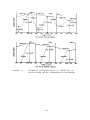
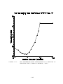
The process of adjusting the vertical profile to reflect
loss of plume mass near the surface is illustrated in Figures
1-6 and 1-7. At a distance far enough downwind that the plume
size in the vertical has grown larger than the height of the
plume, significant corrections to the concentration profile may
be needed to represent the removal of material from the plume
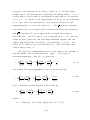
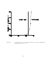
due to deposition. Figure 1-6 displays a depletion factor FQ,
and the corresponding profile correction factor P(z) for a
distance at which Fz is 1.5 times the plume height. The
depletion factor is constant with height, whereas the profile
correction shows that most of the material is lost from the
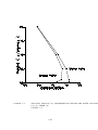
lower portion of the plume. Figure 1-7 compares the vertical
profile of concentration both with and without deposition and
the corresponding depletion of material from the plume. The
depleted plume profile is computed using Equation (1-54).
Both FQ(x) and P(x,z) depend on the size and density of
the particles being modeled, because this effects the total
deposition velocity (See Section 1.3.2). Therefore, for a
given source of particulates, ISC allows multiple particle-size
categories to be defined, with the maximum number of particle
size categories controlled by a parameter statement in the
model code (see Volume I). The user must provide the mass-mean
particle diameter (microns), the particle density (g/cm3), and
the mass fraction (N) for each category being modeled. If we
denote the value of FQ(x) and P(x,z) for the nth particle-size
category by FQn(x) and Pn(x,z) and substitute these in Equation
(1-54), we see that a different value for the vertical term is
obtained for each particle-size category, denoted as Vdn.
Therefore, the total vertical term is given by the sum of the
terms for each particle-size category, weighted by the
respective mass-fractions:
N
Vd x,z,hed ' j Nn Vdn x,z,hed
n'1
1-37
(1-55)
FQ(x) is a function of the total deposition velocity (vd),
V(x,zd,hed), and P(x,zd):
x
F Q(x)
' EXP &
m
vd V x ),zd ,hed P x ),zd dx )
(1-56)
o
where zd is a height near the surface at which the deposition
flux is calculated. The deposition reference height is
calculated as the maximum of 1.0 meters and 20z0. This
equation reflects the fact that the material removed from the
plume by deposition is just the integral of the deposition flux
over the distance that the plume has traveled. In ISC, this
integral is evaluated numerically. For sources modeled in
elevated or complex terrain, the user can input a terrain grid
to the model, which is used to determine the terrain elevation
at various distances along the plume path during the evaluation
of the integral. If a terrain grid is not input by the user,
then the model will linearly interpolate between the source
elevation and the receptor elevation.
The profile correction factor P(x,z) is given by
' P x,zd 1 %
,zd . 1 %
v d & vg
vg
4
m
o
v d & vg
vg
1 & EXP &vg R z,zd
(1-57a)
V x,z ),o
2B Fz
1 & EXP & vg R z ),zd
dz
where R(z,zd) is an atmospheric resistance to vertical
transport that is derived from Briggs' formulas for Fz
(Gifford, 1976). When the product vgR(z,zd) is of order 0.1 or
less, the exponential function is approximated (for small
argument) to simplify P(x,z):
1-38
P( x, z )
• P x,z d
1 % v d & vg R z,zd
4
P x,z d • 1 % v d & vg
m
o
&1
)
V x,z ,o
2B Fz
R z ),z d dz )
(1-57b)
This simplification is important, since the integral in
Equation (1-57a) is evaluated numerically, whereas that in
Equation (1-57b) is computed using analytical approximations.
The resistance R(z,zd) is obtained for the following
functional forms of Fz defined by Briggs:
1-39
Ca s e
1:
Ru r a l :
s t a bi l i t y
A,
Ur b a n :
s t a bi l i t y
C
B
Fz ' a x
R z,z d '
2 1
ln z/z d
B au
Case 2:
Rural: stability C, D
Urban: stability D, E, F
Fz ' a x/ 1 % b x 1/ 2
R z,z d '
2 1
B au
b
a
ln z/z d %
B
z & zd
2
(1&58)
Case 3:
Rural: stability E, F
Fz ' a x/ 1 % b x
R z,z d '
2 1
2b
ln z/z d %
B au
a
B
3b 2
z & zd %
2
2a 2
2
B 2
z & zd
2
Case 4:
Urban: stability A, B
Fz ' a x 1 % b x 1/ 2
R z,z d '
2 1
ln
B au
1 % b x(z) & 1
1 % b x zd % 1
1 % b x(z) % 1
1 % b x zd & 1
For this last form, the x(z) and x(zd) must be solved for z and
zd (respectively) by finding the root of the implicit relation
B
z ' a x
2
1 % bx
1-40
(1-59)
The corresponding functions for P(x,zd) for the special case of
Equation (1-57) are given by:
1-41
Case 1:
Rural: stability A, B
Urban: stability C
Fz ' a x
P &1 x,zd ' 1 %
v d & vg
ua
2
ln
B
2 Fz /z d &1
Case 2:
Rural: stability C, D
Urban: stability D, E, F
Fz ' a x/ 1 % b x 1/ 2
P &1 x,zd ' 1 %
v d & vg
ua
2
B
ln 2Fz /zd &1
Case 3:
Rural: stability E, F
(1-60)
Fz ' a x/ 1 % b x
P &1 x,zd ' 1 %
3b 2
2a 2
v d & vg
2
B
ln 2 Fz /z d & 1
2
B
ln 2 Fz1 /z d &
ua
B 2
2
Fz & zd
2
Case 4:
Urban: stability A, B
Fz ' a x 1 % b x 1/ 2
P &1 x,zd • 1 %
ln
v d & vg
ua
1 % k zd /8 &
2
k Fz2 /8
B
1-42
For the last form, k '
2b
a
B
, and
2
1-43
Fz1 ' Fz 1 & .0006 Fz
2
Fz # 300m
Fz1 ' 0.6724 Fz
Fz > 300m
and
(1-61)
Fz2 ' Fz1
Fz1 # 1000m
Fz2 ' 1000 Fz1
Fz1 > 1000m
The added complexity of this last form arises because a simple
analytical solution to Equation (1-57) could not be obtained
for the urban class A and B. The integral in P(x,zd) for Fz =
ax(1 + bx)1/2 listed above matches a numerical solution to
within about 2% for zd = 1 m.
When vertical mixing is limited by zi, the profile
correction factor P(x,zd) involves an integral from 0 to zi,
rather than from 0 to infinity. Furthermore, V contains terms
that simulate reflection from z = zi as well as z = 0 so that
the profile correction factor, P(x,zd), becomes a function of
mixing height, i.e, P(x,zd,zi). In the well-mixed limit,
P(x,zd,zi) has the same form as P(x,zd) in Equation (1-60) but
Fz is replaced by a constant times zi:
2 Fz /zd
n
B
zd
2
Fz &
6 ln zi /zd
6
B
zi &
8
B
zd
2
(1-62)
2
2
z
&
2
zd
6
2
B
1 2
2
zi & zd
3
.
2 zi
2
& zd
B 3
Therefore a limit is placed on each term involving Fz in
Equation (1-60) so that each term does not exceed the
1-44
corresponding term in zi. Similarly, since the leading order
term in P(x,zd) for Fz = ax(1 + bx)1/2 corresponds to the
ln 2 Fz /z d
term in Equation (1-62), Fz is capped at zi / 2 for
this P(x,zd) as well. Note that these caps to Fz in Equation
(1-60) are broadly consistent with the condition on the use of
the well-mixed limit on V in Equation (1-51) which uses a ratio
Fz/zi = 1.6. In Equation (1-62), the corresponding ratios are
Fz/zi = 1.4, 1.6, and 1.9.
In many applications, the removal of material from the
plume may be extremely small, so that FQ(x) and P(x,z) are
virtually unity. When this happens, the vertical term is
virtually unchanged (Vd = V, see Equation (1-54)). The
deposition flux can then be approximated as vdP rather than
vdPd. The plume depletion calculations are optional, so that
the added expense of computing FQ(x) and P(x,z) can be avoided.
Not considering the effects of dry depletion results in
conservative estimates of both concentration and deposition,
since material deposited on the surface is not removed from the
plume.
1.1.7 The Decay Term (D)
The Decay Term in Equation (1-1) is a simple method of
accounting for pollutant removal by physical or chemical
processes. It is of the form:
D
' exp &R
x
us
for R > 0
(1-63)
or
' 1
for R ' 0
where:
1-45
R
=
the decay coefficient (s-1) (a value of zero means
decay is not considered)
x
=
downwind distance (m)
For example, if T1/2 is the pollutant half life in seconds, the
user can obtain R from the relationship:
R '
0.693
T1/ 2
(1-64)
The default value for R is zero. That is, decay is not
considered in the model calculations unless R is specified.
However, a decay half life of 4 hours (R = 0.0000481 s-1) is
automatically assigned for SO2 when modeled in the urban mode.
1.2 NON-POINT SOURCE EMISSIONS
1.2.1 General
The ISC models include algorithms to model volume, area
and open-pit sources, in addition to point sources. These nonpoint source options of the ISC models are used to simulate the
effects of emissions from a wide variety of industrial sources.
In general, the ISC volume source model is used to simulate the
effects of emissions from sources such as building roof
monitors and line sources (for example, conveyor belts and rail
lines). The ISC area source model is used to simulate the
effects of fugitive emissions from sources such as storage
piles and slag dumps. The ISC open pit source model is used to
simulate fugitive emissions from below-grade open pits, such as
surface coal mines or stone quarries.
1.2.2 The Short-Term Volume Source Model
The ISC models use a virtual point source algorithm to
model the effects of volume sources, which means that an
imaginary or virtual point source is located at a certain
distance upwind of the volume source (called the virtual
distance) to account for the initial size of the volume source
1-46
plume. Therefore, Equation (1-1) is also used to calculate
concentrations produced by volume source emissions.
There are two types of volume sources: surface-based
sources, which may also be modeled as area sources, and
elevated sources. An example of a surface-based source is a
surface rail line. The effective emission height he for a
surface-based source is usually set equal to zero. An example
of an elevated source is an elevated rail line with an
effective emission height he set equal to the height of the
rail line. If the volume source is elevated, the user assigns
the effective emission height he, i.e., there is no plume rise
associated with volume sources. The user also assigns initial
lateral (Fyo) and vertical (Fzo) dimensions for the volume
source. Lateral (xy) and vertical (xz) virtual distances are
added to the actual downwind distance x for the Fy and Fz
calculations. The virtual distances are calculated from
solutions to the sigma equations as is done for point sources
with building downwash.
The volume source model is used to simulate the effects of
emissions from sources such as building roof monitors and for
line sources (for example, conveyor belts and rail lines). The
north-south and east-west dimensions of each volume source used
in the model must be the same. Table 1-6 summarizes the
general procedures suggested for estimating initial lateral
(Fyo) and vertical (Fzo) dimensions for single volume sources
and for multiple volume sources used to represent a line
source. In the case of a long and narrow line source such as a
rail line, it may not be practical to divide the source into N
volume sources, where N is given by the length of the line
source divided by its width. The user can obtain an
approximate representation of the line source by placing a
smaller number of volume sources at equal intervals along the
line source, as shown in Figure 1-8. In general, the spacing
between individual volume sources should not be greater than
1-47
twice the width of the line source. However, a larger spacing
can be used if the ratio of the minimum source-receptor
separation and the spacing between individual volume sources is
greater than about 3. In these cases, concentrations
calculated using fewer than N volume sources to represent the
line source converge to the concentrations calculated using N
volume sources to represent the line source as long as
sufficient volume sources are used to preserve the horizontal
geometry of the line source.
Figure 1-8 illustrates representations of a curved line
source by multiple volume sources. Emissions from a line
source or narrow volume source represented by multiple volume
sources are divided equally among the individual sources unless
there is a known spatial variation in emissions. Setting the
initial lateral dimension Fyo equal to W/2.15 in Figure 1-8(a)
or 2W/2.15 in Figure 1-8(b) results in overlapping Gaussian
distributions for the individual sources. If the wind
direction is normal to a straight line source that is
represented by multiple volume sources, the initial crosswind
concentration distribution is uniform except at the edges of
the line source. The doubling of Fyo by the user in the
approximate line-source representation in Figure 1-8(b) is
offset by the fact that the emission rates for the individual
volume sources are also doubled by the user.
1-48
TABLE 1-6
SUMMARY OF SUGGESTED PROCEDURES FOR ESTIMATING
INITIAL LATERAL DIMENSIONS Fyo AND
INITIAL VERTICAL DIMENSIONS Fzo FOR VOLUME AND LINE SOURCES
Procedure for Obtaining
Initial Dimension
Type of Source
(a)
Initial Lateral Dimensions (Fyo)
Single Volume Source
Fyo =
length of side divided
by 4.3
Line Source Represented by
Adjacent Volume Sources (see
Figure 1-8(a))
Fyo =
length of side divided
by 2.15
Line Source Represented by
Separated Volume Sources (see
Figure 1-8(b))
Fyo =
center to center
distance divided by
2.15
(b)
Initial Vertical Dimensions (Fzo)
Surface-Based Source (he - 0)
Fzo =
vertical dimension of
source divided by 2.15
Elevated Source (he > 0) on or
Adjacent to a Building
Fzo =
building height
divided by 2.15
Elevated Source (he > 0) not
on or Adjacent to a Building
Fzo =
vertical dimension of
source divided by 4.3
1.2.3 The Short-Term Area Source Model
The ISC Short Term area source model is based on a
numerical integration over the area in the upwind and crosswind
directions of the Gaussian point source plume formula given in
Equation (1-1). Individual area sources may be represented as
rectangles with aspect ratios (length/width) of up to 10 to 1.
In addition, the rectangles may be rotated relative to a northsouth and east-west orientation. As shown by Figure 1-9, the
effects of an irregularly shaped area can be simulated by
dividing the area source into multiple areas. Note that the
size and shape of the individual area sources in Figure 1-9
varies; the only requirement is that each area source must be a
1-49
rectangle. As a result, an irregular area source can be
represented by a smaller number of area sources than if each
area had to be a square shape. Because of the flexibility in
specifying elongated area sources with the Short Term model, up
to an aspect ratio of about 10 to 1, the ISCST area source
algorithm may also be useful for modeling certain types of line
sources.
The ground-level concentration at a receptor located
downwind of all or a portion of the source area is given by a
double integral in the upwind (x) and crosswind (y) directions
as:
QAK
VD
2 B us m Fy Fz
P '
x
m
y
exp &0.5
y
Fy
2
dy dx
(1-65)
where:
QA
=
area source emission rate (mass per unit area per
unit time)
K
=
units scaling coefficient (Equation (1-1))
V
=
vertical term (see Section 1.1.6)
D
=
decay term as a function of x (see Section 1.1.7)
The Vertical Term is given by Equation (1-50) or Equation
(1-54) with the effective emission height, he, being the
physical release height assigned by the user. In general, he
should be set equal to the physical height of the source of
emissions above local terrain height. For example, the
emission height he of a slag dump is the physical height of the
slag dump.
Since the ISCST algorithm estimates the integral over the
area upwind of the receptor location, receptors may be located
within the area itself, downwind of the area, or adjacent to
the area. However, since Fz goes to 0 as the downwind distance
goes to 0 (see Section 1.1.5.1), the plume function is infinite
1-50
for a downwind receptor distance of 0. To avoid this
singularity in evaluating the plume function, the model
arbitrarily sets the plume function to 0 when the receptor
distance is less than 1 meter. As a result, the area source
algorithm will not provide reliable results for receptors
located within or adjacent to very small areas, with dimensions
on the order of a few meters across. In these cases, the
receptor should be placed at least 1 meter outside of the area.
In Equation (1-65), the integral in the lateral (i.e.,
crosswind or y) direction is solved analytically as follows:
m
exp &0.5
y
y
Fy
2
dy ' erfc
y
Fy
(1-66)
where erfc is the complementary error function.
In Equation (1-65), the integral in the longitudinal
(i.e., upwind or x) direction is approximated using numerical
methods based on Press, et al (1986). Specifically, the ISCST
model estimates the value of the integral, I, as a weighted
average of previous estimates, using a scaled down
extrapolation as follows:
I
'
VD
erfc
m Fy Fz
x
y
Fy
dx ' I2N%
I2N& IN
3
(1-67)
where the integral term refers to the integral of the plume
function in the upwind direction, and IN and I2N refer to
successive estimates of the integral using a trapezoidal
approximation with N intervals and 2N intervals. The number of
intervals is doubled on successive trapezoidal estimates of the
integral. The ISCST model also performs a Romberg integration
by treating the sequence Ik as a polynomial in k. The Romberg
integration technique is described in detail in Section 4.3 of
Press, et al (1986). The ISCST model uses a set of three
criteria to determine whether the process of integrating in the
upwind direction has "converged." The calculation process will
1-51
be considered to have converged, and the most recent estimate
of the integral used, if any of the following conditions is
true:
1)
if the number of "halving intervals" (N) in the
trapezoidal approximation of the integral has reached
10, where the number of individual elements in the
approximation is given by 1 + 2N-1 = 513 for N of 10;
2)
if the extrapolated estimate of the real integral
(Romberg approximation) has converged to within a
tolerance of 0.0001 (i.e., 0.01 percent), and at
least 4 halving intervals have been completed; or
3)
if the extrapolated estimate of the real integral is
less than 1.0E-10, and at least 4 halving intervals
have been completed.
The first condition essentially puts a time limit on the
integration process, the second condition checks for the
accuracy of the estimate of the integral, and the third
condition places a lower threshold limit on the value of the
integral. The result of these numerical methods is an estimate
of the full integral that is essentially equivalent to, but
much more efficient than, the method of estimating the integral
as a series of line sources, such as the method used by the PAL
2.0 model (Petersen and Rumsey, 1987).
1-52
1.2.4 The Short-Term Open Pit Source Model
The ISC open pit source model is used to estimate impacts
for particulate emissions originating from a below-grade open
pit, such as a surface coal mine or a stone quarry. The ISC
models allow the open pit source to be characterized by a
rectangular shape with an aspect ratio (length/width) of up to
10 to 1. The rectangular pit may also be rotated relative to a
north-south and east-west orientation. Since the open pit
model does not apply to receptors located within the boundary
of the pit, the concentration at those receptors will be set to
zero by the ISC models.
The model accounts for partial retention of emissions
within the pit by calculating an escape fraction for each
particle size category. The variations in escape fractions
across particle sizes result in a modified distribution of mass
escaping from the pit. Fluid modeling has shown that withinpit emissions have a tendency to escape from the upwind side of
the pit. The open pit algorithm simulates the escaping pit
emissions by using an effective rectangular area source using
the ISC area source algorithm described in Section 1.2.3. The
shape, size and location of the effective area source varies
with the wind direction and the relative depth of the pit.
Because the shape and location of the effective area source
varies with wind direction, a single open pit source should not
be subdivided into multiple pit sources.
The escape fraction for each particle size catagory, gi,
is calculated as follows:
gi '
1
(1 % vg /(" U r ))
where:
vg = is the gravitational settling velocity (m/s),
Ur = is the approach wind speed at 10m (m/s),
1-53
(1-68)
"
= is the proportionality constant in the relationship
between flux from the pit and the product of Ur and
concentration in the pit (Thompson, 1994).
The gravitational settling velocity, vg, is computed as
described in Section 1.3.2 for each particle size category.
Thompson (1994) used laboratory measurements of pollutant
residence times in a variety of pit shapes typical of actual
mines and determined that a single value of " = 0.029 worked
well for all pits studied.
The adjusted emission rate (Qi) for each particle size
category is then computed as:
Qi ' gi @Ni @ Q
(1-69)
where Q is the total emission rate (for all particles) within
the pit, Ni is the original mass fraction for the given size
category, and g is the escape fraction calculated from Equation
(1-68). The adjusted total emission rate (for all particles
escaping the pit), Qa, is the sum of the Qi for all particle
categories calculated from Equation 1-69. The mass fractions
(of particles escaping the pit), Nai, for each category is:
Nai ' Q i / Qa
(1-70)
Because of particle settling within the pit, the distribution
of mass escaping the pit is different than that emitted within
the pit. The adjusted total particulate emission rate, Qa, and
the adjusted mass fractions, Nai, reflect this change, and it
is these adjusted values that are used for modeling the open
pit emissions.
The following describes the specification of the location,
dimensions and adjusted emissions for the effective area source
1-54
used for modeling open pit emissions. Consider an arbitrary
rectangular-shaped pit with an arbitrary wind direction as
shown in Figure 1-10. The steps that the model uses for
determining the effective area source are as follows:
1.
Determine the upwind sides of the pit based on the
wind direction.
2.
Compute the along wind length of the pit (R) based on
the wind direction and the pit geometry . R varies
between the lengths of the two sides of the
rectangular pit as follows:
R ' L@(1 & 2/90) % W@(2/90)
(1-71)
where L is the long axis and W is the short axis of
the pit, and 2 is the wind direction relative to the
long axis (L) of the pit (therefore 2 varies between
0E and 90E). Note that with this formulation and a
square pit, the value of R will remain constant with
wind direction at R = L = W. The along wind
dimension, R, is the scaling factor used to normalize
the depth of the pit.
3.
4.
The user specifies the average height of emissions
from the floor of the pit (H) and the pit volume (V).
The effective pit depth (de) and the relative pit
depth (Dr) are then calculated as follows:
de ' V/(L@W)
(1-72)
Dr ' (de &H)/R
(1-73)
Based on observations and measurements in a wind
tunnel study (Perry, et al., 1994), it is clear that
the emissions within the pit are not uniformly
released from the pit opening. Rather, the emissions
show a tendency to be emitted primarily from an
upwind sub-area of the pit opening. Therefore an
effective area source (with Ae being the fractional
size relative to the entire pit opening) is used to
simulate the pit emissions. Ae represents a single
area source whose dimensions and location depend on
the effective depth of the pit and the wind
direction. Based on wind tunnel results, if Dr$0.2,
then the effective area is about 8% of the total
opening of the mine (i.e. Ae=0.08). If Dr<0.2, then
the fractional area increases as follows:
1-55
e
1/ 3 1/ 2
' (1.0&1.7Dr
)
(1-74)
When Dr = 0, which means that the height of emissions
above the floor equals the effective depth of the
pit, the effective area is equal to the total area of
the mine opening (i.e. Ae=1.0).
Having determined the effective area from which the model
will simulate the pit emissions, the specific dimensions of
this effective rectangular area are calculated as a function of
2 such that (see Figure 1-10):
AW
2
( 1&cos
' Ae
θ)
(1-75)
@W
and
( cos
AL ' Ae
2
θ)
@L
(1-76)
Note that in equations 1-75 and 1-76, W is defined as the short
dimension of the pit and L is the long dimension; AW is the
dimension of the effective area aligned with the short side of
the pit and AL is the dimension of the effective area aligned
with the long side of the pit (see Figure 1-10). The
dimensions AW and AL are used by the model to define the shape
of the effective area for input to the area source algorithm
described in Section 1.2.3.
The emission rate, Qe, for the effective area is such that
Qe ' Q a /Ae
(1-77)
where Qa is the emission rate per unit area (from the pit after
adjustment for escape fraction) if the emissions were uniformly
released from the actual pit opening (with an area of L@W).
That is, if the effective area is one-third of the total area,
1-56
then the emission rate (per unit area) used for the effective
area is three times that from the full area.
Because of the high level of turbulence in the mine, the
pollutant is initially mixed prior to exiting the pit.
Therefore some initial vertical dispersion is included to
represent this in the effective area source. Using the
effective pit depth, de, as the representative dimension over
which the pollutant is vertically mixed in the pit, the initial
vertical dispersion value, Fzo, is equal to de/4.3. Note that
4.3@Fzo represents about 90% of a Gaussian plume (in the
vertical), so that the mixing in the pit is assumed to
approximately equal the mixing in a plume.
Therefore, for the effective area source representing the
pit emissions, the initial dispersion is included with ambient
dispersion as:
2
2
Fz ' (Fzo % Fz (x))1/ 2
(1-78)
For receptors close to the pit, the initial dispersion value
can be particularly important.
Once the model has determined the characteristics of the
effective area used to model pit emissions for a particular
hour, the area source algorithm described in Section 1.2.3 is
used to calculate the concentration or deposition flux values
at the receptors being modeled.
1.3 THE ISC SHORT-TERM DRY DEPOSITION MODEL
1.3.1 General
This section describes the ISC Short Term dry deposition
model, which is used to calculate the amount of material
1-57
deposited (i.e., the deposition flux, Fd) at the surface from a
particle plume through dry deposition processes.
The Short Term dry deposition model is based on a dry
deposition algorithm (Pleim et al., 1984) contained in the Acid
Deposition and Oxidant Model (ADOM). This algorithm was
selected as a result of an independent model evaluation study
(EPA, 1994).
The deposition flux, Fd, is calculated as the product of
the concentration, Pd, and a deposition velocity, vd, computed
at a reference height zd:
Fd
' Pd @ v d
(1-79)
The concentration value, Pd, used in Equation (1-79) is
calculated according to Equation (1-1) with deposition effects
accounted for in the vertical term as described in Section
1.1.6.3. The calculation of deposition velocities is described
below.
1.3.2 Deposition Velocities
A resistance method is used to calculate the deposition
velocity, vd. The general approach used in the resistance
methods for estimating vd is to include explicit
parameterizations of the effects of Brownian motion, inertial
impaction, and gravitational settling. The deposition velocity
is written as the inverse of a sum of resistances to pollutant
transfer through various layers, plus gravitational settling
terms (Slinn and Slinn, 1980; Pleim et al., 1984):
v d
where,
vd
'
1
% vg
ra % rd % ra rd vg
=
the deposition velocity (cm/s),
1-58
(1-80)
=
=
=
vg
ra
rd
the gravitational settling velocity (cm/s),
the aerodynamic resistance (s/cm), and,
the deposition layer resistance (s/cm).
Note that for large settling velocities, the deposition
velocity approaches the settling velocity (vd 6 vg), whereas,
for small settling velocities, vd tends to be dominated by the
ra and rd resistance terms.
In addition to the mass mean diameters (microns), particle
densities (gm/cm3), and the mass fractions for each particle
size category being modeled, the dry deposition model also
requires surface roughness length (cm), friction velocity
(m/s), and Monin-Obukhov length (m). The surface roughness
length is specified by the user, and the meteorological
preprocessor (PCRAMMET or MPRM) calculates the friction
velocity and Monin-Obukhov length for input to the model.
The lowest few meters of the atmosphere can be divided
into two layers: a fully turbulent region where vertical fluxes
are nearly constant, and the thin quasi-laminar sublayer. The
resistance to transport through the turbulent, constant flux
layer is the aerodynamic resistance. It is usually assumed
that the eddy diffusivity for mass transfer within this layer
is similar to that for heat. The atmospheric resistance
formulation is based on Byun and Dennis (1995):
stable (L > 0):
r a
'
1
ln
k u(
zd
zo
% 4.7
z
L
(1-81)
unstable (L < 0):
'
( 1 % 16 (z/*L*) & 1) ( 1 % 16 (z0 /*L*) % 1
1
ln
k u(
( 1 % 16 (z/*L*) % 1) ( 1 % 16 (z0 /*L*) & 1
1-59
(1-82)
where,
u*
k
z
L
zd
zo
=
=
=
=
=
=
the surface friction velocity (cm/s),
the von Karman constant (0.4),
the height above ground (m),
the Monin-Obukhov length (m),
deposition reference height (m), and
the surface roughness length (m).
The coefficients used in the atmospheric resistance formulation
are those suggested by Dyer (1974). A minimum value for L of
1.0m is used for rural locations. Recommended minimum values
for urban areas are provided in the user's guides for the
meteorological preprocessor programs PCRAMMET and MPRM.
The approach used by Pleim et al. (1984) to parameterize
the deposition layer resistance terms is modified to include
Slinn's (1982) estimate for the inertial impaction term. The
resulting deposition layer resistance is:
rd '
where,
1
Sc &2/ 3 % 10&3/ St u(
(1-83)
Sc
=
the Schmidt number (Sc = L/DB)
(dimensionless),
L
=
the viscosity of air (• 0.15 cm2/s),
DB
=
the Brownian diffusivity (cm2/s) of the
pollutant in air,
St
=
the Stokes number [St = (vg/g)(u*2 /L)]
(dimensionless),
g
=
the acceleration due to gravity (981 cm/s2),
The gravitational settling velocity, vg (cm/s), is
calculated as:
1-60
2
g
where,
S CF
'
D & DAIR g dp c2
18µ
SCF
(1-84)
D
=
the particle density (g/cm3),
DAIR
=
the air density (• 1.2 x 10-3 g/cm3),
dp
=
the particle diameter (µm),
µ
=
the absolute viscosity of air (• 1.81 x 10-4
g/cm/s),
c2
=
air units conversion constant (1 x 10-8
cm2/µm2), and
SCF
=
the slip correction factor, which is computed
as:
' 1. %
2x2 a1 % a2 e
& a 3 d p / x2
(1-85)
10&4 dp
and, x2, a1, a2, a3 are constants with values of 6.5 x 10-6,
1.257, 0.4, and 0.55 x 10-4, respectively.
The Brownian diffusivity of the pollutant (in cm/s) is
computed from the following relationship:
DB
' 8.09 x 10&10
Ta SCF
(1-86)
dp
where Ta is the air temperature (EK).
The first term of Eqn. (1-83), involving the Schmidt
number, parameterizes the effects of Brownian motion. This
term controls the deposition rate for small particles. The
second term, involving the Stokes number, is a measure of the
importance of inertial impaction, which tends to dominate for
1-61
intermediate-sized particles in the 2-20 µm diameter size
range.
The deposition algorithm also allows a small adjustment to
the deposition rates to account for possible phoretic effects.
Some examples of phoretic effects (Hicks, 1982) are:
THERMOPHORESIS:
Particles close to a hot surface experience a
force directed away from the surface because, on the
average, the air molecules impacting on the side of the
particle facing the surface are hotter and more energetic.
DIFFUSIOPHORESIS: Close to an evaporating surface, a particle
is more likely to be impacted by water molecules on the
side of the particle facing the surface. Since the water
molecules have a lower molecular weight than the average
air molecule, there is a net force toward the surface,
which results in a small enhancement of the deposition
velocity of the particle.
A second effect is that the impaction of new water vapor
molecules at an evaporating surface displaces a certain
volume of air. For example, 18 g of water vapor
evaporating from 1 m2 will displace 22.4 liters of air at
standard temperature and pressure (STP) conditions (Hicks,
1982). This effect is called Stefan flow. The Stefan
flow effect tends to reduce deposition fluxes from an
evaporating surface. Conversely, deposition fluxes to a
surface experiencing condensation will be enhanced.
ELECTROPHORESIS: Attractive electrical forces have the
potential to assist the transport of small particles
through the quasi-laminar deposition layer, and thus could
increase the deposition velocity in situations with high
local field strengths. However, Hicks (1982) suggests
this effect is likely to be small in most natural
circumstances.
Phoretic and Stefan flow effects are generally small.
However, for particles in the range of 0.1 - 1.0 µm diameter,
which have low deposition velocities, these effects may not
always be negligible. Therefore, the ability to specify a
phoretic term to the deposition velocity is added (i.e., vdN =
vd + vd(phor), where vdN is the modified deposition velocity and
vd(phor) is the phoretic term).
1-62
Although the magnitude and sign of vd(phor) will vary, a
small, constant value of + 0.01 cm/s is used in the present
implementation of the model to represent combined phoretic
effects.
1-63
1.3.3 Point and Volume Source Emissions
As stated in Equation (1-59), deposition is modeled as the
product of the near-surface concentration (from Equation (1-1))
times the deposition velocity (from Equation (1-80)).
Therefore, the vertical term given in Equation (1-54) that is
used to obtain the concentration at height z, subject to
particle settling and deposition, can be evaluated at height zd
for one particle size, and multiplied by a deposition velocity
for that particle size to obtain a corresponding "vertical
term" for deposition. Since more than one particle size
category is typically used, the deposition for the nth size
category must also include the mass fraction for the category:
Fdn
' P d n @ vd n
'
Qτ K Nn vd n Vd n x,zd ,hed D
2B Fy Fz u s
exp &0.5
y
Fy
2
(1-87)
where K, N, Vd, and D were defined previously (Equations (1-1),
(1-54), and (1-63)). The parameter QJ is the total amount of
material emitted during the time period J for which the
deposition calculation is made. For example, QJ is the total
amount of material emitted during a 1-hour period if an hourly
deposition is calculated. To simplify the user input, and to
keep the maximum compatibility between input files for
concentration and deposition runs, the model takes emission
inputs in grams per second (g/s), and converts to grams per
hour for deposition calculations. For time periods longer than
an hour, the program sums the deposition calculated for each
hour to obtain the total deposition flux for the period. In
the case of a volume source, the user must specify the
effective emission height he and the initial source dimensions
Fyo and Fzo. It should be noted that for computational
1-64
NPD
purposes, the model calculates the quantity, j Nn vdn Vdn , as
n'l
the "vertical term."
1.3.4 Area and Open Pit Source Emissions
For area and open pit source emissions, Equation (1-65) is
changed to the form:
Fdn
' Pd n @ vd n
'
QAτ K Nn vd n
2 B us
Vd n D
m Fy Fz
x
m
y
exp &0.5
y
Fy
(1-88)
2
dy dx
where K, D, Vd, and vd are defined in Equations (1-1), (1-54),
(1-65), and (1-80). The parameter QAJ is the total mass per
unit area emitted over the time period J for which deposition
is calculated. The area source integral is estimated as
described in Section 1.2.3.
1.4 THE ISC SHORT-TERM WET DEPOSITION MODEL
A scavenging ratio approach is used to model the
deposition of gases and particles through wet removal. In this
approach, the flux of material to the surface through wet
deposition (Fw) is the product of a scavenging ratio times the
concentration, integrated in the vertical:
4
Fw x , y '
m
7 P x , y , z dz
(1-89)
o
where the scavenging ratio (7) has units of s-1. The
concentration value is calculated using Equation (1-1). Since
the precipitation is assumed to initiate above the plume
height, a wet deposition flux is calculated even if the plume
height exceeds the mixing height. Across the plume, the total
1-65
flux to the surface must equal the mass lost from the plume so
that
%4
d
&
Q (x) '
F (x , y) dy ' 7 Q (x) / u
m w
dx
(1-90)
&4
Solving this equation for Q(x), the source depletion
relationship is obtained as follows:
Q (x) ' Q o e &Λx / u ' Qo e &Λt
(1-91)
where t = x/u is the plume travel time in seconds. As with dry
deposition (Section 1.3), the ratio Q(x)/Qo is computed as a
wet depletion factor, which is applied to the flux term in
Equation (1-89). The wet depletion calculation is also
optional. Not considering the effects of wet depletion will
result in conservative estimates of both concentration and
deposition, since material deposited on the surface is not
removed from the plume.
The scavenging ratio is computed from a scavenging
coefficient and a precipitation rate (Scire et al., 1990):
7 ' 8 @ R
(1-92)
where the coefficient 8 has units (s-mm/hr)-1, and the
precipitation rate R has units (mm/hr). The scavenging
coefficient depends on the characteristics of the pollutant
(e.g., solubility and reactivity for gases, size distribution
for particles) as well as the nature of the precipitation
(e.g., liquid or frozen). Jindal and Heinold (1991) have
analyzed particle scavenging data reported by Radke et al.
(1980), and found that the linear relationship of Equation
(1-90) provides a better fit to the data than the non-linear
assumption 7 = 8Rb. Furthermore, they report best-fit values
for 8 as a function of particle size. These values of the
scavenging rate coefficient are displayed in Figure 1-11.
1-66
Although the largest particle size included in the study is 10
µm, the authors suggest that 8 should reach a plateau beyond 10
µm, as shown in Figure 1-11. The scavenging rate coefficients
for frozen precipitation are expected to be reduced to about
1/3 of the values in Figure 1-11 based on data for sulfate and
nitrate (Scire et al., 1990). The scavenging rate coefficients
are input to the model by the user.
The wet deposition algorithm requires precipitation type
(liquid or solid) and precipitation rate, which is prepared for
input to the model through the meteorological preprocessor
programs (PCRAMMET or MPRM).
1.5 ISC COMPLEX TERRAIN SCREENING ALGORITHMS
The Short Term model uses a steady-state, sector-averaged
Gaussian plume equation for applications in complex terrain
(i.e., terrain above stack or release height). Terrain below
release height is referred to as simple terrain; receptors
located in simple terrain are modeled with the point source
model described in Section 1.1. The sector average approach
used in complex terrain implies that the lateral (crosswind)
distribution of concentrations is uniform across a 22.5 degree
sector. The complex terrain screening algorithms apply only to
point source and volume source emissions; area source and open
pit emission sources are excluded. The complex terrain point
source model, which is based on the COMPLEX1 model, is
described below. The description parallels the discussion for
the simple terrain algorithm in Section 1.1, and includes the
basic Gaussian sector-average equation, the plume rise
formulas, and the formulas used for determining dispersion
parameters.
1-67
1.5.1 The Gaussian Sector Average Equation
The Short Term complex terrain screening algorithm for
stacks uses the steady-state, sector-averaged Gaussian plume
equation for a continuous elevated source. As with the simple
terrain algorithm described in Section 1.1, the origin of the
source's coordinate system is placed at the ground surface at
the base of the stack for each source and each hour. The x
axis is positive in the downwind direction, the y axis is
crosswind (normal) to the x axis and the z axis extends
vertically. The fixed receptor locations are converted to each
source's coordinate system for each hourly concentration
calculation. Since the concentrations are uniform across a
22.5 degree sector, the complex terrain algorithms use the
radial distance between source and receptor instead of downwind
distance. The calculation of the downwind, crosswind and
radial distances is described in Section 1.5.2. The hourly
concentrations calculated for each source at each receptor are
summed to obtain the total concentration produced at each
receptor by the combined source emissions.
For a Gaussian, sector-averaged plume, the hourly
concentration at downwind distance x (meters) and crosswind
distance y (meters) is given by:
P '
QKVD
2B R ) 2´ us Fz
@ CORR
(1-93)
where:
Q
=
pollutant emission rate (mass per unit time),
K
=
units scaling coefficient (see Equation (1-1))
)2´
=
the sector width in radians (=0.3927)
R
=
radial distance from the point source to the
receptor = [(x+xy)2 + y2]1/2 (m)
x
=
downwind distance from source center to
receptor, measured along the plume axis (m)
1-68
y
=
lateral distance from the plume axis to the
receptor (m)
xy
=
lateral virtual distance for volume sources (see
Equation (1-35)), equals zero for point sources
(m)
us
=
mean wind speed (m/sec) at stack height
Fz
=
standard deviation of the vertical concentration
distribution (m)
V
=
the Vertical Term (see Section 1.1.6)
D
=
the Decay Term (see Section 1.1.7)
CORR
=
the attenuation correction factor for receptors
above the plume centerline height (see Section
1.5.8)
Equation (1-93) includes a Vertical Term, a Decay Term,
and a vertical dispersion term (Fz). The Vertical Term
includes the effects of source elevation, receptor elevation,
plume rise, limited vertical mixing, gravitational settling and
dry deposition.
1.5.2 Downwind, Crosswind and Radial Distances
The calculation of downwind and crosswind distances is
described in Section 1.1.2. Since the complex terrain
algorithms in ISC are based on a sector average, the radial
distance is used in calculating the plume rise (see Section
1.5.4) and dispersion parameters (see Section 1.5.5). The
radial distance is calculated as R = [x2 + y2]1/2, where x is the
downwind distance and y is the crosswind distance described in
Section 1.1.2.
1.5.3 Wind Speed Profile
See the discussion given in Section 1.1.3.
1.5.4 Plume Rise Formulas
The complex terrain algorithm in ISC uses the Briggs plume
rise equations described in Section 1.1.4. For distances less
1-69
than the distance to final rise, the complex terrain algorithm
uses the distance-dependent plume height (based on the radial
distance) as described in Section 1.1.4.10. Since the complex
terrain algorithm does not incorporate the effects of building
downwash, the Schulman-Scire plume rise described in Section
1.1.4.11 is not used for complex terrain modeling. The plume
height is used in the calculation of the Vertical Term
described in Section 1.5.6.
1.5.5 The Dispersion Parameters
The dispersion parameters used in the complex terrain
algorithms of ISC are the same as the point source dispersion
parameters for the simple terrain algorithms described in
Section 1.1.5.1, except that the radial distance is used
instead of the downwind distance. Since the lateral
distribution of the plume in complex terrain is determined by
the sector average approach, the complex terrain algorithm does
not use the lateral dispersion parameter, Fy. The procedure to
account for buoyancy-induced dispersion in the complex terrain
algorithm only affects the vertical dispersion term (see
Equation 1-48). Since the complex terrain algorithm does not
incorporate the effects of building downwash, the enhanced
dispersion parameters and virtual distances do not apply.
1.5.6 The Vertical Term
The Vertical Term used in the complex terrain algorithm in
ISC is the same as described in Section 1.1.6 for the simple
terrain algorithm, except that the plume height and dispersion
parameter input to the vertical term are based on the radial
distance, as described above, and that the adjustment of plume
height for terrain above stack base is different, as described
in Section 1.5.6.1.
1-70
1.5.6.1 The Vertical Term in Complex Terrain.
The ISC complex terrain algorithm makes the following
assumption about plume behavior in complex terrain:
$
The plume axis remains at the plume stabilization
height above mean sea level as it passes over complex
terrain for stable conditions (categories E and F), and
uses a "half-height" correction factor for unstable and
neutral conditions (categories A - D).
$
The plume centerline height is never less than 10 m
above the ground level in complex terrain.
$
The mixing height is terrain following, i.e, the mixing
height above ground at the receptor location is assumed
to be the same as the height above ground at the source
location.
$
The wind speed is a function of height above the
surface (see Equation (1-6)).
Thus, a modified plume stabilization height he´ is
substituted for the effective stack height he in the Vertical
Term given by Equation (1-50). The effective plume
stabilization height at the point x,y is given by:
he ´ ' h e & (1&FT) H t
(1-94)
where:
he
= plume height at point x,y without terrain
adjustment, as described in Section 1.5.4 (m)
Ht
= z*(x,y) - zs = terrain height of the receptor
location above the base of the stack (m)
z*(x,y)
= height above mean sea level of terrain at the
receptor location (x,y) (m)
zs
= height above mean sea level of the base of the
stack (m)
FT
= terrain adjustment factor, which is 0.5 for
stability categories A - D and 0.0 for stability
categories E and F.
1-71
The effect of the terrain adjustment factor is that the plume
height relative to stack base is deflected upwards by an amount
equal to half of the terrain height as it passes over complex
terrain during unstable and neutral conditions. The plume
height is not deflected by the terrain under stable conditions.
1.5.6.2
The Vertical Term for Particle Deposition
The Vertical Term for particle deposition used in the
complex terrain algorithm in ISC is the same as described in
Section 1.1.6 for the simple terrain algorithm, except that the
plume height and dispersion parameter input to the vertical
term are based on the radial distance, as described above, and
that the adjustment of plume height for terrain above stack
base is different, as described in Section 1.5.6.2.
1.5.7 The Decay Term
See the discussion given in Section 1.1.7.
1.5.8 The Plume Attenuation Correction Factor
Deflection of the plume by complex terrain features during
stable conditions is simulated by applying an attenuation
correction factor to the concentration with height in the
sector of concern. This is represented by the variable CORR in
Equation (1-93). The attenuation correction factor has a value
of unity for receptors located at and below the elevation of
the plume centerline in free air prior to encountering terrain
effects, and decreases linearly with increasing height of the
receptor above plume level to a value of zero for receptors
located at least 400 m above the undisturded plume centerline
height. This relationship is shown in the following equation:
1-72
C OR R
' 1.0
unstable/neutral
' 1.0
)H r # 0m
(1-95)
' 0.0
' (400&)Hr )/400
where:
CORR
)Hr
)Hr $ 400m
)Hr < 400m
= attenuation correction factor, which is between 0
and 1
= height of receptor above undisturbed plume height,
including height of receptor above local ground
(i.e., flagpole height)
1.5.9 Wet Deposition in Complex Terrain
See the discussion given in Section 1.4.
1.6 ISC TREATMENT OF INTERMEDIATE TERRAIN
In the ISC Short Term model, intermediate terrain is
defined as terrain that exceeds the height of the release, but
is below the plume centerline height. The plume centerline
height used to define whether a given receptor is on
intermediate terrain is the distance-dependent plume height
calculated for the complex terrain algorithm, before the
terrain adjustment (Section 1.5.6.2) is applied.
If the plume height is equal to or exceeds the terrain
height, then that receptor is defined as complex terrain for
that hour and that source, and the concentration is based on
the complex terrain screening algorithm only. If the terrain
1-73
height is below the plume height but exceeds the physical
release height, then that receptor is defined as intermediate
terrain for that hour and source. For intermediate terrain
receptors, concentrations from both the simple terrain
algorithm and the complex terrain algorithm are obtained and
the higher of the two concentrations is used for that hour and
that source. If the terrain height is less than or equal to
the physical release height, then that receptor is defined as
simple terrain, and the concentration is based on the simple
terrain algorithm only.
For deposition calculations, the intermediate terrain
analysis is first applied to the concentrations at a given
receptor, and the algorithm (simple or complex) that gives the
highest concentration at that receptor is used to calculate the
deposition value.
1-74
FIGURE 1-1.
LINEAR DECAY FACTOR, A AS A FUNCTION OF
EFFECTIVE STACK HEIGHT, He. A SQUAT BUILDING IS
ASSUMED FOR SIMPLICITY.
1-75
FIGURE 1-2.
ILLUSTRATION OF TWO TIERED BUILDING WITH
DIFFERENT TIERS DOMINATING DIFFERENT WIND
DIRECTIONS
1-76
FIGURE 1-3.
THE METHOD OF MULTIPLE PLUME IMAGES USED TO
SIMULATE PLUME REFLECTION IN THE ISC2 MODEL
1-77
FIGURE 1-4.
SCHEMATIC ILLUSTRATION OF (a) URBAN AND (b)
RURAL MIXING HEIGHT INTERPOLATION PROCEDURES
1-78
FIGURE 1-5.
ILLUSTRATION OF PLUME BEHAVIOR IN ELEVATED
TERRAIN ASSUMED BY THE ISC2 MODEL
1-79
FIGURE 1-6.
ILLUSTRATION OF THE DEPLETION FACTOR FQ AND THE CORRESPONDI
CORRECTION FACTOR P(x,z).
1-80
FIGURE 1-7.
VERTICAL PROFILE OF CONCENTRATION BEFORE AND AFTER APPLYIN
P(x,z) SHOWN IN
FIGURE 1-6.
1-81
FIGURE 1-8.
EXACT AND APPROXIMATE REPRESENTATIONS OF A LINE
SOURCE BY MULTIPLE VOLUME SOURCES
1-82
1
2
3
4
FIGURE 1-9.
REPRESENTATION OF AN IRREGULARLY SHAPED AREA
SOURCE BY 4 RECTANGULAR AREA SOURCES
1-83
Wind direction
O
effective
area
2
AW
W
1
3
alongwind
length (l)
AL
4
L
FIGURE 1-10.
EFFECTIVE AREA AND ALONGWIND WIDTH FOR AN OPEN
PIT SOURCE
1-84
FIGURE 1-11.
WET SCAVENGING RATE COEFFICIENT AS A FUNCTION OF
PARTICLE SIZE (JINDAL & HEINOLD, 1991)
1-85
2.0 THE ISC LONG-TERM DISPERSION MODEL EQUATIONS
This section describes the ISC Long-Term model equations.
Where the technical information is the same, this section
refers to the ISC Short-Term model description in Section 1 for
details. The long-term model provides options for modeling the
same types of sources as provided by the short-term model. The
information provided below follows the same order as used for
the short-term model equations.
The ISC long-term model uses input meteorological data
that have been summarized into joint frequencies of occurrence
for particular wind speed classes, wind direction sectors, and
stability categories. These summaries, called STAR summaries
for STability ARray, may include frequency distributions over a
monthly, seasonal or annual basis. The long term model has the
option of calculating concentration or dry deposition values
for each separate STAR summary input and/or for the combined
period covered by all available STAR summaries. Since the wind
direction input is the frequency of occurrence over a sector,
with no information on the distribution of winds within the
sector, the ISC long-term model uses a Gaussian sector-average
plume equation as the basis for modeling pollutant emissions on
a long-term basis.
2.1 POINT SOURCE EMISSIONS
2.1.1 The Gaussian Sector Average Equation
The ISC long-term model makes the same basic assumption as
the short-term model. In the long-term model, the area
surrounding a continuous source of pollutants is divided into
sectors of equal angular width corresponding to the sectors of
the seasonal and annual frequency distributions of wind
direction, wind speed, and stability. Seasonal or annual
emissions from the source are partitioned among the sectors
according to the frequencies of wind blowing toward the
2-1
sectors. The concentration fields calculated for each source
are translated to a common coordinate system (either polar or
Cartesian as specified by the user) and summed to obtain the
total due to all sources.
For a single stack, the mean seasonal concentration is
given by:
Pl '
K
2B R ) 2´
j
i,j,k
QfSVD
u s Fz
(2-1)
where:
K
=
units scaling coefficient (see Equation (1-1))
Q
=
pollutant emission rate (mass per unit time),
for the ith wind-speed category, the kth
stability category and the lth season
f
=
frequency of occurrence of the ith wind-speed
category, the jth wind-direction category and
the kth stability category for the lth season
)2´
=
the sector width in radians
R
=
radial distance from lateral virtual point
source (for building downwash) to the receptor =
[(x+xy)2 + y2]1/2 (m)
x
=
downwind distance from source center to
receptor, measured along the plume axis (m)
y
=
lateral distance from the plume axis to the
receptor (m)
xy
=
lateral virtual distance (see Equation (1-35)),
equals zero for point sources without building
downwash, and for downwash sources that do not
experience lateral dispersion enhancement (m)
S
=
a smoothing function similar to that of the AQDM
(see Section 2.1.8)
us
=
mean wind speed (m/sec) at stack height for the
ith wind-speed category and kth stability
category
2-2
Fz
=
standard deviation of the vertical concentration
distribution (m) for the kth stability category
V
=
the Vertical Term for the ith wind-speed
category, kth stability category and lth season
D
=
the Decay Term for the ith wind speed category
and kth stability category
The mean annual concentration at the point (r,2) is
calculated from the seasonal concentrations using the
expression:
4
Pa ' 0.25 j Pl
(2-2)
l '1
The terms in Equation (2-1) correspond to the terms
discussed in Section 1.1 for the short-term model except that
the parameters are defined for discrete categories of
wind-speed, wind-direction, stability and season. The various
terms are briefly discussed in the following subsections. In
addition to point source emissions, the ISC long-term
concentration model considers emissions from volume and area
sources. These model options are discussed in Section 2.2.
The optional algorithms for calculating dry deposition are
discussed in Section 2.3.
2.1.2 Downwind and Crosswind Distances
See the discussion given in Section 1.1.2.
2.1.3 Wind Speed Profile
See the discussion given in Section 1.1.3.
2.1.4 Plume Rise Formulas
See the discussion given in Section 1.1.4.
2-3
2.1.5 The Dispersion Parameters
2.1.5.1 Point Source Dispersion Parameters.
See Section 1.1.5.1 for a discussion of the procedures use
to calculate the standard deviation of the vertical
concentration distribution Fz for point sources (sources
without initial dimensions). Since the long term model assumes
a uniform lateral distribution across the sector width, the
model does not use the standard deviation of the lateral
dispersion, Fy (except for use with the Schulman-Scire plume
rise formulas described in Section 1.1.4.11).
2.1.5.2 Lateral and Vertical Virtual Distances.
See Section 1.1.5.2 for a discussion of the procedures
used to calculate vertical virtual distances. The lateral
virtual distance is given by:
Py ' ro cot
) 2´
2
(2-3)
where ro is the effective source radius in meters. For volume
sources (see Section 2.2.2), the program sets ro equal to
2.15Fyo, where Fyo is the initial lateral dimension. For area
sources (see Section 2.2.3), the program sets ro equal to xo/ B
where xo is the length of the side of the area source. For
plumes affected by building wakes (see Section 1.1.5.2), the
program sets ro equal to 2.15 Fy´ where Fy´ is given for squat
buildings by Equation (1-41), (1-42), or (1-43) for downwind
distances between 3 and 10 building heights and for tall
buildings by Equation (1-44) for downwind distances between 3
and 10 building widths. At downwind distances greater than 10
building heights for Equation (1-41), (1-42), or (1-43), Fy´ is
held constant at the value of Fy´ calculated at a downwind
distance of 10 building heights. Similarly, at downwind
distances greater than 10 building widths for Equation (1-44),
2-4
Fy´ is held constant at the value of Fy´ calculated at a
downwind distance of 10 building widths.
2.1.5.3 Procedures Used to Account for the Effects of
Building Wakes on Effluent Dispersion.
With the exception of the equations used to calculate the
lateral virtual distance, the procedures used to account for
the effects of building wake effects on effluent dispersion are
the same as those outlined in Section 1.1.5.3 for the
short-term model. The calculation of lateral virtual distances
by the long-term model is discussed in Section 2.1.5.2 above.
2.1.5.4 Procedures Used to Account for Buoyancy-Induced
Dispersion.
See the discussion given in Section 1.1.5.4.
2.1.6 The Vertical Term
2.1.6.1 The Vertical Term for Gases and Small
Particulates.
Except for the use of seasons and discrete categories of
wind-speed and stability, the Vertical Term for gases and small
particulates corresponds to the short term version discussed in
Section 1.1.6. The user may assign a separate mixing height zi
to each combination of wind-speed and stability category for
each season.
As with the Short-Term model, the Vertical Term is changed
to the form:
'
2BFz
(2-4)
zi
at downwind distances where the Fz/zi ratio is greater than or
equal to 1.6. Additionally, the ground-level concentration is
set equal to zero if the effective stack height he exceeds the
mixing height zi. As explained in Section 1.1.6.1, the ISC
2-5
model currently assumes unlimited mixing for the E and F
stability categories.
2.1.6.2 The Vertical Term in Elevated Terrain.
See the discussion given in Section 1.1.6.2.
2.1.6.3 The Vertical Term for Large Particulates.
Section 1.1.6.3 discusses the differences in the
dispersion of large particulates and the dispersion of gases
and small particulates and provides the guidance on the use of
this option. The Vertical Term for large particulates is given
by Equation (1-53).
2.1.7 The Decay Term
See the discussion given in Section 1.1.7.
2.1.8 The Smoothing Function
As shown by Equation (2-1), the rectangular concentration
distribution within a given angular sector is modified by the
function S{2} which smooths discontinuities in the
concentration at the boundaries of adjacent sectors. The
centerline concentration in each sector is unaffected by
contribution from adjacent sectors. At points off the sector
centerline, the concentration is a weighted function of the
concentration at the centerline and the concentration at the
centerline of the nearest adjoining sector. The smoothing
function is given by:
S
'
()2´ & *2j ´ & 2´*)
)2)
for *2j ´ & 2´*
(2-5)
or
' 0
for *2j ´ & 2´*
2-6
where:
2 j´
=
the angle measured in radians from north to the
centerline of the jth wind-direction sector
2´
=
the angle measured in radians from north to the
receptor point (R, 2) where R, defined above for
equation 2-1, is measured from the lateral virtual
source.
2.2 NON-POINT SOURCE EMISSIONS
2.2.1 General
As explained in Section 1.2.1, the ISC volume, area and
open pit sources are used to simulate the effects of emissions
from a wide variety of industrial sources. Section 1.2.2
provides a description of the volume source model, Section
1.2.3 provides a description of the area source model, and
Section 1.2.4 provides a description of the open pit model.
The following subsections give the volume, area and open pit
source equations used by the long-term model.
2.2.2 The Long-Term Volume Source Model
The ISC Long Term Model uses a virtual point source
algorithm to model the effects of volume sources. Therefore,
Equation (2-1) is also used to calculate seasonal average
ground-level concentrations for volume source emissions. The
user must assign initial lateral (Fyo) and vertical (Fzo)
dimensions and the effective emission height he. A discussion
of the application of the volume source model is given in
Section 1.2.2.
2.2.3 The Long-Term Area Source Model
The ISC Long Term Area Source Model is based on the
numerical integration algorithm for modeling area sources used
by the ISC Short Term model, which is described in detail in
Section 1.2.3. For each combination of wind speed class,
2-7
stability category and wind direction sector in the STAR
meteorological frequency summary, the ISC Long Term model
calculates a sector average concentration by integrating the
results from the ISC Short Term area source algorithm across
the sector. A trapezoidal integration is used, as follows:
N&1
f(2)P(2)d2
(fi1 P(2i1 )%fi NP(2i N))
1
m
Pi '
[ j fij P(2ij )%
'
]% ,(2)
N j '1
S
2
(2-6a)LD (2; P
6b)
where:
Pi
=
the sector average concentration value for the
ith sector
S
=
the sector width
fij
=
the frequency of occurrence for the jth wind
direction in the ith sector
,(2)
=
the error term - a criterion of ,(2) < 2 percent
is used to check for convergence of the sector
average calculation
P(2ij)
=
the concentration value, based on the numerical
integration algorithm using Equation (1-58) for
the jth wind direction in the ith sector
2ij
=
the jth wind direction in the ith sector, j = 1
and N correspond to the two boundaries of the
sector.
The application of Equation (2-6a) to calculate the sector
average concentration from area sources is an iterative
process. Calculations using the ISC Short Term algorithm
(Equation (1-58)) are initially made for three wind directions,
corresponding to the two boundaries of the sector and the
centerline direction. The algorithm then calculates the
concentration for wind directions midway between the three
directions, for a total of five directions, and calculates the
2-8
error term. If the error is less than 2 percent, then the
concentration based on five directions is used to represent the
sector average, otherwise, additional wind directions are
selected midway between each of the five directions and the
process continued. This process continues until the
convergence criteria, described below, are satisfied.
In order to avoid abrupt changes in the concentrations at
the sector boundaries with the numerical integration algorithm,
a linear interpolation is used to determine the frequency of
occurrence of each wind direction used for the individual
simulations within a sector, based on the frequencies of
occurrence in the adjacent sectors. This "smoothing" of the
frequency distribution has a similar effect as the smoothing
function used for the ISC Long Term point source algorithm,
described in Section 2.1.8. The frequency of occurrence of the
jth wind direction between sectors i and i+1 can be calculated
as:
fij ' Fi %(1i %1 &2ij )
(Fi %1 &F i )
(1i %1 &1i )
(2-6c)
where:
Fi
=
the frequency of occurrence for the ith sector
Fi+1
=
the frequency of occurrence for the i+1th sector
1i
=
the central wind direction for the ith sector
1i+1
=
the central wind direction for the i+1th sector
2ij
=
the specific wind direction between 1i and 1i+1
fij
=
the interpolated (smoothed) frequency of
occurrence for the specific wind direction 2ij
The ISCLT model uses a set of three criteria to determine
whether the process of calculating the sector average
concentration has "converged." The calculation process will be
2-9
considered to have converged, and the most recent estimate of
the trapezoidal integral used, if any of the following
conditions is true:
1)
if the number of "halving intervals" (N) in the
trapezoidal approximation of the sector average has
reached 10, where the number of individual elements
in the approximation is given by 1 + 2N-1 = 513 for N
of 10;
2)
if the estimate of the sector average has converged
to within a tolerance of 0.02 (i.e., 2 percent), for
two successive iterations, and at least 2 halving
intervals have been completed (a minimum of 5 wind
direction simulations); or
3)
if the estimate of the sector average concentration
is less than 1.0E-10, and at least 2 halving
intervals have been completed.
The first condition essentially puts a time limit on the
integration process, the second condition checks for the
accuracy of the estimate of the sector average, and the third
condition places a lower threshold limit that avoids
convergence problems associated with very small concentrations
where truncation error may be significant.
2-10
2.2.4 The Long-Term Open Pit Source Model
The ISC Long Term Open Pit Source Model is based on the
use of the long term area source model described in Section
2.2.3. The escape fractions and adjusted mass distribution for
particle emissions from an open pit, and the determination of
the size, shape and location of the effective area source used
to model open pit emissions are described in Section 1.2.4.
For the Long Term model, a sector average value for open pit
sources is calculated by determining an effective area for a
range of wind directions within the sector and increasing the
number of wind directions used until the result converges, as
described in Section 2.2.3 for the Long Term area source model.
The contribution from each effective area used within a sector
is calculated using the Short Term area source model described
in Section 1.2.3.
2.3 THE ISC LONG-TERM DRY DEPOSITION MODEL
2.3.1 General
The concepts upon which the ISC long-term dry deposition
model are based are discussed in Sections 1.1.6.3 and 1.3.
2.3.2 Point and Volume Source Emissions
The seasonal deposition at the point located at a
particular distance (r) and direction (2) with respect to the
base of a stack or the center of a volume source for
particulates in the nth particle size category is given by:
Fd
l,n
'
K Nn
2B R 2 ) 2´
j
i, j, k
Qτ f S Vd n D
Fz
(2-7)
where the vertical term for deposition, Vdn, was defined in
Section 1.3.2. K and D are described in Equations (1-1) and
(1-63), respectively. QJ is the product of the total time
during the lth season, of the seasonal emission rate Q for the
2-11
ith wind-speed category, kth stability category. For example,
if the emission rate is in grams per second and there are 92
days in the summer season (June, July, and August), QJ,l-3 is
given by 7.95 x 106 Ql-3. It should be noted that the user need
not vary the emission rate by season or by wind speed and
stability. If an annual average emission rate is assumed, QJ
is equal to 3.15 x 107 Q for a 365-day year. For a plume
comprised of N particle size categories, the total seasonal
deposition is obtained by summing Equation (2-7) over the N
particle size categories. The program also sums the seasonal
deposition values to obtain the annual deposition.
2.3.3 Area and Open Pit Source Emissions
The area and open pit source dry deposition calculations
for the ISCLT model are based on the numerical integration
algorithm for modeling area sources used by the ISCST model.
Section 1.3.3, Equation (1-61), describes the numerical
integration for the Short Term model that is applied to
specific wind directions by the Long Term model in a
trapezoidal integration to calculate the sector average. The
process of calculating sector averages for area sources in the
Long Term model is described by Equation (2-6) in Section
2.2.3.
2-12
3.0 REFERENCES
Bowers, J.F., J.R. Bjorklund and C.S. Cheney, 1979: Industrial
Source Complex (ISC) Dispersion Model User's Guide. Volume
I, EPA-450/4-79-030, U.S. Environmental Protection Agency,
Research Triangle Park, North Carolina 27711.
Bowers, J.R., J.R. Bjorklund and C.S. Cheney, 1979: Industrial
Source Complex (ISC) Dispersion Model User's Guide. Volume
II, EPA-450/4-79-031, U.S. Environmental Protection
Agency, Research Triangle Park, North Carolina 27711.
Briggs, G.A., 1969, Plume Rise, USAEC Critical Review Series,
TID-25075, National Technical Information Service,
Springfield, Virginia 22161.
Briggs, G.A., 1979: Some Recent Analyses of Plume Rise
Observations, In Proceedings of the Second International
Clean Air Congress, Academic Press, New York.
Briggs, G.A., 1972: Discussion on Chimney Plumes in Neutral
and Stable Surroundings. Atmos. Environ., 6, 507-510.
Briggs, G.A., 1974: Diffusion Estimation for Small Emissions.
In ERL, ARL USAEC Report ATDL-106. U.S. Atomic Energy
Commission, Oak Ridge, Tennessee.
Briggs, G.A., 1975: Plume Rise Predications. In Lectures on
Air Pollution and Environmental Impact Analysis, American
Meteorological Society, Boston, Massachusetts.
Byun, D.W. and R. Dennis, 1995: Design Artifacts in Eulerian
Air Quality Models: Evaluation of the Effects of Layer
Thickness and Vertical Profile Correction on Surface Ozone
Concentrations. Atmos. Environ., 29, 105-126.
Chico, T. and J.A. Catalano, 1986: Addendum to the User's
Guide for MPTER. Contract No. EPA 68-02-4106, U.S.
Environmental Protection Agency, Research Triangle Park,
North Carolina 27711.
Cramer, H.E., et al., 1972: Development of Dosage Models and
Concepts. Final Report Under Contract DAAD09-67-C-0020(R)
with the U.S. Army, Desert Test Center Report DTC-TR-609,
Fort Douglas, Utah.
Dumbauld, R.K. and J.R. Bjorklund, 1975: NASA/MSFC Multilayer
Diffusion Models and Computer Programs -- Version 5. NASA
Contractor Report No. NASA CR-2631, National Aeronautics
and Space Administration, George C. Marshall Space Center,
Alabama.
3-1
Dyer, A.J., 1974: A review of flux-profile relationships.
Boundary-Layer Meteorol., 7, 363-372.
Environmental Protection Agency, 1985: Guideline for
Determination of Good Engineering Practice Stack Height
(Technical Support Document for the Stack Height
Regulations) - Revised, EPA-450/4-80-023R, U.S.
Environmental Protection Agency, Research Triangle Park,
NC 27711. (NTIS No. PB 85-225241)
Environmental Protection Agency, 1992. Comparison of a Revised
Area Source Algorithm for the Industrial Source Complex
Short Term Model and Wind Tunnel Data. EPA Publication
No. EPA-454/R-92-014. U.S. Environmental Protection
Agency, Research Triangle Park, NC. (NTIS No. PB 93226751)
Environmental Protection Agency, 1992. Sensitivity Analysis of
a Revised Area Source Algorithm for the Industrial Source
Complex Short Term Model. EPA Publication No. EPA-454/R92-015. U.S. Environmental Protection Agency, Research
Triangle Park, NC. (NTIS No. PB 93-226769)
Environmental Protection Agency, 1992. Development and
Evaluation of a Revised Area Source Algorithm for the
Industrial Source Complex Long Term Model. EPA
Publication No. EPA-454/R-92-016. U.S. Environ-mental
Protection Agency, Research Triangle Park, NC. (NTIS No.
PB 93-226777)
Environmental Protection Agency, 1994. Development and Testing
of a Dry Deposition Algorithm (Revised). EPA Publication
No. EPA-454/R-94-015. U.S. Environmental Protection
Agency, Research Triangle Park, NC. (NTIS No. PB 94183100)
Gifford, F.A., Jr. 1976: Turbulent Diffusion - Typing Schemes:
A Review. Nucl. Saf., 17, 68-86.
Hicks, B.B., 1982: Critical assessment document on acid
deposition. ATDL Contrib. File No. 81/24, Atmos. Turb.
and Diff. Laboratory, Oak Ridge, TN.
Holzworth, G.C., 1972: Mixing Heights, Wind Speeds and
Potential for Urban Air Pollution Throughout the
Contiguous United States. Publication No. AP-101, U.S.
Environmental Protection Agency, Research Triangle Park,
North Carolina 27711.
Horst, T.W., 1983: A correction to the Gaussian sourcedepletion model. In Precipitation Scavenging, Dry
Deposition and Resuspension, H.R. Pruppacher, R.G.
Semonin, W.G.N. Slinn, eds., Elsevier, NY.
3-2
Huber, A.H. and W.H. Snyder, 1976: Building Wake Effects on
Short Stack Effluents. Preprint Volume for the Third
Symposium on Atmospheric Diffusion and Air Quality,
American Meteorological Society, Boston, Massachusetts.
Huber, A.H. and W.H. Snyder, 1982. Wind tunnel investigation
of the effects of a rectangular-shaped building on
dispersion of effluents from short adjacent stacks. Atmos.
Environ., 176, 2837-2848.
Huber, A.H., 1977: Incorporating Building/Terrain Wake Effects
on Stack Effluents. Preprint Volume for the Joint
Conference on Applications of Air Pollution Meteorology,
American Meteorological Society, Boston, Massachusetts.
Jindal, M. and D. Heinold, 1991: Development of particulate
scavenging coefficients to model wet deposition from
industrial combustion sources. Paper 91-59.7, 84th Annual
Meeting - Exhibition of AWMA, Vancouver, BC, June 16-21,
1991.
McDonald, J.E., 1960: An Aid to Computation of Terminal Fall
Velocities of Spheres. J. Met., 17, 463.
McElroy, J.L. and F. Pooler, 1968: The St. Louis Dispersion
Study. U.S. Public Health Service, National Air Pollution
Control Administration, Report AP-53.
National Climatic Center, 1970: Card Deck 144 WBAN Hourly
Surface Observations Reference Manual 1970, Available from
the National Climatic Data Center, Asheville, North
Carolina 28801.
Pasquill, F., 1976: Atmospheric Dispersion Parameters in
Gaussian Plume Modeling. Part II. Possible Requirements
for Change in the Turner Workbook Values.
EPA-600/4-76-030b, U.S. Environmental Protection Agency,
Research Triangle Park, North Carolina 27711.
Perry, S.G., R.S. Thompson, and W.B. Petersen, 1994:
Considerations for Modeling Small-Particulate Impacts from
Surface Coal Mining Operations Based on Wind-Tunnel
Simulations. Proceedings Eighth Joint Conference on
Applications of Air Pollution Meteorology, January 23-28,
Nashville, TN.
Petersen, W.B. and E.D. Rumsey, 1987: User's Guide for PAL 2.0
- A Gaussian-Plume Algorithm for Point, Area, and Line
Sources, EPA/600/8-87/009, U.S. Environmental Protection
Agency, Research Triangle Park, North Carolina.
Pleim, J., A. Venkatram and R. Yamartino, 1984: ADOM/TADAP
model development program. Volume 4. The dry deposition
3-3
module. Ontario Ministry of the Environment, Rexdale,
Ontario.
Press, W., B. Flannery, S. Teukolsky, and W. Vetterling, 1986:
Numerical Recipes, Cambridge University Press, New York,
797 pp.
Schulman, L.L. and S.R. Hanna, 1986: Evaluation of Downwash
Modifications to the Industrial Source Complex Model. J.
Air Poll. Control Assoc., 36 (3), 258-264.
Schulman, L.L. and J.S. Scire, 1980: Buoyant Line and Point
Source (BLP) Dispersion Model User's Guide. Document
P-7304B, Environmental Research and Technology, Inc.,
Concord, MA.
Scire, J.S. and L.L. Schulman, 1980: Modeling Plume Rise from
Low-Level Buoyant Line and Point Sources. Proceedings
Second Joint Conference on Applications of Air Pollution
Meteorology, 24-28 March, New Orleans, LA. 133-139.
Scire, J.S., D.G. Strimaitis and R.J. Yamartino, 1990: Model
formulation and user's guide for the CALPUFF dispersion
model. Sigma Research Corp., Concord, MA.
Slinn, W.G.N., 1982: Predictions for particle deposition to
vegetative canopies. Atmos. Environ., 16, 1785-1794.
Slinn, S.A. and W.G.N. Slinn, 1980:
deposition and natural waters.
1016.
Predictions for particle
Atmos. Environ., 14, 1013-
Thompson, R.S., 1994: Residence Time of Contaminants Released
in Surface Coal Mines -- A Wind Tunnel Study. Proceedings
Eighth Joint Conference on Applications of Air Pollution
Meteorology, January 23-28, Nashville, TN.
Touma, J.S., J.S. Irwin, J.A. Tikvart, and C.T. Coulter, 1995.
A Review of Procedures for Updating Air Quality Modeling
Techniques for Regulatory Modeling Programs. J. App.
Meteor., 34, 731-737.
Turner, D.B., 1970: Workbook of Atmospheric Dispersion
Estimates. PHS Publication No. 999-AP-26. U.S.
Department of Health, Education and Welfare, National Air
Pollution Control Administration, Cincinnati, Ohio.
Yamartino, R.J., J.S. Scire, S.R. Hanna, G.R. Carmichael and
Y.S. Chang, 1992: The CALGRID mesoscale photochemical
grid model. Volume I. Model formulation. Atmos.
Environ., 26A, 1493-1512.
3-4
INDEX
Area source
deposition algorithm . .
for the Long Term model
for the Short Term model
Atmospheric resistance . . .
Attenuation correction factor
in complex terrain . . .
.
.
.
.
.
.
.
.
.
.
.
.
.
.
.
.
.
.
.
.
.
.
.
.
.
.
.
.
.
.
.
.
.
.
.
.
.
.
.
.
. 1-61, 2-12
. . . . . 2-7
. 1-43, 1-46
. 1-38, 1-56
. . . . . . . . . . . . . .
Briggs plume rise formulas
buoyant plume rise . . . . . . .
momentum plume rise . . . . . .
stack tip downwash . . . . . . .
Building downwash procedures . . . .
and buoyancy-induced dispersion
effects on dispersion parameters
for the Long Term model . . . .
general . . . . . . . . . . . .
Huber and Snyder . . . . . . . .
Schulman and Scire . . . . . . .
Schulman-Scire plume rise . . .
virtual distances . . . . . . .
wake plume height . . . . . . .
Buoyancy flux . . . . . . . . . . . .
Buoyancy-induced dispersion . . . . .
Buoyant plume rise
stable . . . . . . . . . . . . .
unstable and neutral . . . . . .
Cartesian receptor network . . . . .
Complex terrain modeling
Short Term model . . . . . . . .
Crossover temperature difference . .
Crosswind distance . . . . . . 1-2,
.
.
.
.
.
.
.
.
.
.
.
.
.
.
.
. . . . . . 1-7, 1-9
. . . . . . 1-8, 1-10
. . . . . . . . . 1-6
. . . . . . 1-23, 2-4
. . . . . . . . 1-30
. . . . . . . . 1-21
. 1-64, 2-2, 2-4, 2-5
. . . . . . 1-5, 1-22
. . . . . . . . 1-23
1-5, 1-12, 1-28, 1-29
. . . . . 1-12, 1-14
. . . . . . . . 1-20
. . . . . . . . 1-11
. . . . . . 1-6, 1-13
. . . . . . 1-30, 2-5
. . . . . . . . . . . 1-9
. . . . . . . . . . . 1-7
. . . . . . . . . . . 1-3
. . . . . . . 1-63, 1-69
. . . . . . . . . . . 1-7
1-3, 1-4, 1-64, 1-65, 2-3
Decay coefficient . . . . . . . . . . .
Decay term . . . . . . . . . . . . . .
for the Long Term model . . . . .
for the Short Term model . . . . .
Depletion
for the dry deposition algorithm .
for the wet deposition algorithm .
Deposition layer resistance . . . . . .
Deposition velocity . . . . . . . . . .
Direction-specific building dimensions
with Huber-Snyder downwash . . . .
Dispersion coefficients
see Dispersion parameters . . . .
Dispersion parameters
for the Long Term model . . . . .
McElroy-Pooler . . . . . . . . . .
Pasquill-Gifford . . . . . . . . .
INDEX-1
.
.
.
.
.
.
.
.
.
.
.
.
.
.
.
1-68
.
.
.
.
.
.
.
.
.
.
.
.
. . . . . . 1-42
. 1-3, 1-42, 1-65
. 1-65, 2-3, 2-6
. . . 1-42, 1-68
.
.
.
.
.
.
.
.
.
.
.
.
.
.
.
.
.
.
.
.
.
.
.
.
.
.
.
.
.
.
. 1-35,
. . . .
. . . .
. 1-34,
. 1-22,
. . . .
. . . . . .
1-42
1-62
1-57
1-55
1-29
1-29
1-14, 1-66
. . . . . . . . . . 2-4
. . . . . . 1-15, 1-19
1-14, 1-16, 1-17, 1-18
Distance-dependent plume rise . . . .
Downwind distance . . . . . . . 1-2,
and virtual distance . . . . . .
for area sources . . . . . . . .
for building wake dispersion . .
for dispersion coefficients . .
Dry deposition . . . . . . . . . . .
for the Long Term model . . . .
for the Short Term model . . . .
. . . . .
1-3, 1-4,
. . . . .
. . . . .
. . . . .
. . . . .
. . . . .
. . . . .
. . . . .
. . . . . 1-13
1-64, 1-65, 2-3
. . . . . 1-20
. . . . . 1-47
. . . . . 1-24
. . . . . 1-14
1-3, 1-65, 2-11
. . . . . 2-11
. . . . . 1-54
Elevated terrain . . . . . . . . . . . . . . . 1-33, 1-67, 2-6
truncation above stack height . . . . . . . . . . . 1-34
Entrainment coefficient . . . . . . . . . . . . . . . . . 1-14
Final plume rise . . . .
distance to . . . .
stable . . . . . . .
unstable or neutral
Flagpole receptor . . . .
.
.
.
.
.
.
.
.
.
.
.
.
.
.
.
.
.
.
.
.
.
.
.
.
.
.
.
.
.
.
.
.
.
.
.
.
.
.
.
.
.
.
.
.
.
.
.
.
.
.
.
.
.
.
.
.
.
.
.
.
.
.
.
.
.
.
.
.
.
.
. . 1-30
. . . 1-7
1-9, 1-10
1-7, 1-8
. . 1-32
Gaussian plume model . . . . . . . . . .
sector averages for complex terrain
sector averages for Long Term . . .
GEP stack height . . . . . . . . . . . .
Gradual plume rise . . . . . . . . . . .
for buoyant plumes . . . . . . . . .
for Schulman-Scire downwash . . . .
stable momentum . . . . . . . . . .
unstable and neutral momentum . . .
used for wake plume height . . . . .
.
.
.
.
.
.
.
.
.
.
.
.
.
.
.
.
.
.
.
.
.
.
.
.
.
.
.
.
.
.
.
.
.
.
.
.
.
.
.
.
.
.
.
.
.
.
.
.
.
.
. 1-2, 1-63
. . . 1-63
. . . . 2-1
1-12, 1-29
. . . 1-10
. . . 1-10
. . . 1-13
. . . 1-11
. . . 1-11
. . . 1-11
Half life . . . . . . . . . . . . . . . . . . . . . . . . 1-43
Huber-Snyder downwash algorithm . . . . . . . . . . . . . . 1-5
Initial lateral dimension
for the Long Term model
for volume sources . . .
Initial plume length
Schulman-Scire downwash
Initial plume radius
Schulman-Scire downwash
Initial vertical dimension
for volume sources . . .
Intermediate terrain . . . .
. . . . . . . . . . . . . . . 2-4
. . . . . . . . . . . 1-45, 1-46
. . . . . . . . . . . . . .
1-12
. . . . . . . . . . . . . .
1-13
. . . . . . . . . . . . . .
. . . . . . . . . . . . . .
1-46
1-69
Jet entrainment coefficient . . . . . . . . . . . .
Lateral dispersion parameters
for the Long Term model
Lateral virtual distance
for the Long Term model
Lateral virtual distances
for building downwash .
1-11, 1-14
. . . . . . . . 1-16, 1-19, 1-30
. . . . . . . . . . . . . . . 2-4
. . . . . . . . .
1-64, 2-2, 2-4
. . . . . . . . . . . . . .
INDEX-2
1-26
Line source
approximation for Schulman-Scire sources .
Line sources, modeled as volumes . 1-43, 1-44,
Linear decay factor
Schulman-Scire downwash . . . . . . . . .
Long-term dispersion model . . . . . . . . . .
. . 1-12, 1-13
1-45, 1-46, 2-7
. . 1-13, 1-29
. . . . . . 2-1
McElroy-Pooler dispersion parameters
see Dispersion parameters . . .
Mixing heights . . . . . . . . . . .
Momentum flux . . . . . . . . . . . .
Momentum plume rise . . . . . . . . .
stable . . . . . . . . . . . . .
unstable and neutral . . . . . .
.
.
.
.
.
.
.
.
.
.
.
.
.
.
.
.
.
.
.
.
.
.
.
.
. . . . . . 1-19
. . . . . . 1-33
. . . . 1-6, 1-13
1-11, 1-23, 1-29
. . . . . . 1-10
. . . . . . . 1-8
Open pit source
deposition algorithm . .
for the Long Term model
for the Short Term model
Open pit sources . . . . . .
.
.
.
.
.
.
.
.
.
.
.
.
.
.
.
.
.
.
.
.
.
.
.
.
.
.
.
.
.
.
.
.
.
.
.
.
Pasquill-Gifford dispersion parameters
see Dispersion parameters . . . .
Plume rise
for Schulman-Scire downwash . . .
for the Long Term model . . . . .
for the Short Term model . . . . .
Point source
deposition algorithm . . . . . . .
dispersion parameters . . . . . .
for the Long Term model . . . . .
for the Short Term model . . . . .
Polar receptor network . . . . . . . .
.
.
.
.
. 1-61,
. . . .
. . . .
. 1-43,
. . . . . . . . .
2-12
2-11
1-50
1-50
1-16
. . . . . . . . . 1-12
. . . . . . . . . . 2-3
. . . . . . . 1-5, 1-65
.
.
.
.
.
.
.
.
.
.
.
.
.
.
.
.
.
.
.
.
.
.
.
.
.
.
.
.
.
.
.
.
.
.
1-60, 2-11
1-14, 2-4
. . . 2-1
. . . 1-2
. . . 1-3
Receptors
calculation of source-receptor distances . . . . 1-3, 1-4
Rural
dispersion parameters . . . . . . . . . . . . . . . 1-14
virtual distances . . . . . . . . . . . . . . 1-20, 1-25
Schulman-Scire downwash algorithm
Short-term dispersion model . . .
Sigma-y . . . . . . . . . . . . .
Sigma-z . . . . . . . . . . . . .
Smoothing function
for the Long Term model . .
Stability parameter . . . . . . .
Stack-tip downwash . . . . . . .
for wake plume height . . .
.
.
.
.
.
.
.
.
.
.
.
.
.
.
.
.
.
.
.
.
.
.
.
.
.
.
.
.
.
.
.
.
. . . . . 1-5
. . . . . 1-1
. 1-14, 1-66
. 1-14, 1-66
.
.
.
.
.
.
.
.
.
.
.
.
.
.
.
.
.
.
.
.
.
.
.
.
.
.
.
.
.
.
.
.
.
.
.
.
. 2-2, 2-6
. 1-8, 1-14
. . . . 1-6
. . . 1-12
Uniform vertical mixing . . . . . . . . . . . . . . . . .
Urban
decay term for SO2 . . . . . . . . . . . . . . . . .
INDEX-3
1-32
1-43
dispersion parameters . . . . . . . . . . . . . . . 1-15
virtual distances . . . . . . . . . . . . . . 1-20, 1-25
Vertical dispersion parameters . . . . . . . 1-17, 1-18, 1-19
Vertical term . . . . . . . . . . . . . . 1-3, 1-47, 1-65, 2-5
for gases and small particulates . . . . . . . . . . 1-31
for large particulates . . . . . . . . . . . . . . . . 2-6
for the Long Term model . . . . . . . . . 1-65, 2-3, 2-5
for the Short Term model . . . . . . . . . . . 1-31, 1-66
for uniform vertical mixing . . . . . . . . . . . . 1-32
in complex terrain . . . . . . . . . . . . . . . . . 1-67
in elevated terrain . . . . . . . . . . . . . . 1-33, 2-6
Vertical virtual distances
for building downwash . . . . . . . . . . . . 1-24, 1-25
Virtual distances . . . . . 1-20, 1-21, 1-28, 1-29, 1-44, 1-47
for the Long Term model . . . . . . . . . . . . 2-4, 2-5
for volume sources . . . . . . . . . . . . . . . . . 1-44
Virtual point source . . . . . . . . . . 1-43, 1-64, 2-2, 2-7
Volume source . . . . . . . . . . . . . . . . . . . . . . 1-46
deposition algorithm . . . . . . . . . . . . . 1-60, 2-11
for the Long Term model . . . . . . . . . . . . . . . 2-7
for the Short Term model . . . . . . . . . . . . . . 1-43
Wet deposition
for the Short Term model . . . . . . . . . . . . . . 1-61
Wind speed
minimum wind speed for modeling . . . . . . . . . . . 1-5
Wind speed profile . . . . . . . . . . . . . . 1-4, 1-65, 2-3
INDEX-4
ADDENDUM
USER'S GUIDE FOR THE
INDUSTRIAL SOURCE COMPLEX (ISC3) DISPERSION MODELS
VOLUME II - DESCRIPTION OF MODEL ALGORITHMS
U.S. ENVIRONMENTAL PROTECTION AGENCY
Office of Air Quality Planning and Standards
Emissions, Monitoring, and Analysis Division
Research Triangle Park, North Carolina 27711
June 1999
ACKNOWLEDGMENTS
The Addendum to the User's Guide for the ISC3 Models has been prepared by
Roger W. Brode of Pacific Environmental Services, Inc., Research Triangle Park, North
Carolina, under subcontract to EC/R, Inc., Chapel Hill, North Carolina. This effort has been
funded by the Environmental Protection Agency under Contract No. 68D98006, with Dennis
G. Atkinson as Work Assignment Manager.
INDEX-vi
TECHNICAL DESCRIPTION FOR THE
REVISED ISCST3 MODEL (DATED 99155)
This document provides a technical description of model algorithms for recent
enhancements of the ISCST3 model, including the most recent version dated 99155. The
algorithms described in this Addendum include the gas dry deposition algorithms based on the
draft GDISCDFT model (dated 96248), and the optimizations of the area source algorithm.
Both of these enhancements are associated with the non-regulatory default TOXICS option
introduced with version 99155 of ISCST3. A brief description of the user instructions for these
new options is presented in the accompanying Addendum to Volume I of the ISC3 model
user’s guide (ISC3ADD1.WPD).
Gas Dry Deposition Algorithms
The ISCST3 dry deposition algorithm for gaseous pollutants is based on the algorithm
contained in the CALPUFF dispersion model (EPA, 1995a), and has undergone limited review
and evaluation (Moore, at al. 1995).
The deposition flux, Fd, is calculated as the product of the concentration, χd, and a
deposition velocity, vd, computed at a reference height zd:
F d ' Pd @ v d
(A1)
The concentration value, χd, used in Equation A1 is calculated according to Equation 1-1 of the
ISC3 model user’s guide, Volume II (EPA, 1995b), with deposition effects accounted for in
the vertical term as described in Section 1.1.6.3 of Volume II. The calculation of deposition
velocities is described below for gaseous emissions.
Deposition Velocities for Gases
At a reference height zd, the deposition velocity (vd) for gases is expressed (Wesley and
Hicks, 1977; Hicks, 1982) as the inverse of a sum of three resistances:
vd ' r a % rd % r c
where, ra
&1
=
the atmospheric resistance (s/m) through the surface layer,
rd
=
the deposition layer resistance (s/m), and,
rc
=
the canopy (vegetation layer) resistance (s/m).
INDEX-1
(A2)
An alternative pathway that is potentially important in sparsely vegetated areas or over water is
deposition directly to the ground/water surface. Although not involving vegetation, it is
convenient to include the ground/water surface resistance as a component of rc.
The atmospheric resistance term (ra) is given by Equations 1-81 and 1-82 in Section
1.3.2 of the ISC3 model user’s guide, Volume II (EPA, 1995b).
The deposition layer resistance (rd) is parameterized in terms of the Schmidt number
(EPA, 1995a) as:
d2
r d ' d1 S c / k u (
where, Sc
(A3)
=
the Schmidt number (υ/DM),
υ
=
the kinematic viscosity of air (~0.15 × 10-4 m2/s),
DM
=
the molecular diffusivity of the pollutant (m2/s), and,
=
empirical parameters; d1/k=5, d2=2/3 (Hicks, 1982)
k
=
the von Karman constant (~0.4)
u*
=
surface friction velocity (m/s)
d1, d2
The canopy resistance (rc) is the resistance for gases in the vegetation layer, including
the ground/water surface. There are three main pathways for uptake/reaction within the
vegetation or at the surface (EPA, 1995a):
(1)
Transfer through the stomatal pore and dissolution or reaction in the mesophyll cells
(plant tissue that contains chlorophyll).
(2)
Reaction with or transfer through the leaf cuticle.
(3)
Transfer into the ground/water surface.
These pathways are treated as three resistances in parallel.
rc ' LAI / rf % LAI / rcut % 1 / rg &1
INDEX-2
(A4)
where, rf
=
the internal foliage resistance (s/m) (Pathway 1, Transfer through the
stomatal pore and dissolution or reaction in mesophyll cells),
rcut
=
the cuticle resistance (s/m), (Pathway 2, Reaction with or transfer
through the leaf cuticle, a thin film covering the surface of plants),
rg
=
the ground or water surface resistance (s/m), (Pathway 3, Transfer
into the ground/water surface), and,
LAI
=
the leaf area index (ratio of leaf surface area divided by ground
surface area). The LAI is specified as a function of wind direction
and month/season, and is included in the meteorological input file
provided by the MPRM preprocessor.
Pathway 1:
The internal foliage resistance (rf) consists of two components:
rf ' r s % rm
where, rs
(A5)
=
the resistance (s/m) to transport through the stomatal pore (see below),
and,
rm
=
the resistance (s/m) to dissolution or reaction of the pollutant in the
mesophyll (spongy parenchyma) cells, user input by species. For
soluble compounds (HF, SO2, CL2, NH3), set to zero; for less
soluble compounds (NO2), it could be > 0)
Stomatal opening/closing is a response to the plant's competing needs for uptake of
CO2 and prevention of water loss from the leaves. Stomatal action imposes a strong diurnal
cycle on the stomatal resistance, and has an important role in determining deposition rates for
soluble gaseous pollutants such as SO2. Stomatal resistance (rs) is given by (EPA, 1995a):
rs ' p s / (b DM)
where, ps
(A6)
=
a stomatal constant corresponding to the characteristics of leaf
physiology (• 2.3 x 10-8 m2),
b
=
the width of the stomatal opening (m), and,
DM
=
the molecular diffusivity of the pollutant (m2/s).
INDEX-3
The width of the stomatal opening (b) is a function of the radiation intensity, moisture
availability, and temperature. In ISC3, the state of vegetation is specified as one of three
states: (A) active and unstressed, (B) active and stressed, or (C) inactive. Irrigated vegetation
can be assumed to be in an active and unstressed state. The variation in stomatal opening
width during period (A) when vegetation is active and unstressed (Pleim et al., 1984) is:
b ' bmax R I / Rmax % bmin
where, bmax
(A7)
=
the maximum width (m) of the stomatal opening (- 2.5 x 10-6 m) (Padro
et al., 1991),
bmin
=
the minimum width (m) of the stomatal opening (- 0.1 x 10-6 m),
RI
=
the incoming solar radiation (W/m2) received at the ground, and is
included in the meteorological input file for the model by the
MPRM preprocessor, and,
Rmax
=
the incoming solar radiation (W/m2) at which full opening of the
stomata occur; assume constant and equal to 600.
During periods of moisture stress, the need to prevent moisture loss becomes critical,
and the stomata close. Thus for period (B), active vegetation under moisture stress conditions,
assume that b = bmin. When vegetation is inactive (e.g., during the seasonal dry period), the
internal foliage resistance becomes very large, essentially cutting off Pathway 1.
Assuming the vegetation is in state (A), active and unstressed, ambient temperature
provides an additional bound on the value of rs. During cold periods (T<10EC), metabolic
activity slows, and b is set by the code to bmin. During hot weather conditions (T>~35EC) the
stomata are fully open (b=bmax) to allow evaporative cooling of the plant.
Pathway 2:
The resistance due to reaction with or transfer through the leaf cuticle (rcut) is given by
(EPA, 1995a):
rcut ' Aref / AR rcut ref
where, Aref
(A8)
=
the reference reactivity parameter of SO2 (- 8.0),
AR
=
the reactivity parameter for the depositing gas, (NO2=8, O3=15,
HNO3=18, PAN=4), and,
=
the empirically determined reference cuticle resistance (s/m) of
SO2, set equal to 3000 s/m (Padro et al., 1991).
rcut(ref)
INDEX-4
Pathway 3:
The third resistance pathway for rc is transfer into the ground/water surface (rg). In
sparsely vegetated areas, deposition directly to the surface may be an important pathway.
r g ' Aref / AR rg ref
where, rg(ref) =
(A9)
the reference resistance of SO2 over ground (- 1000 s/m) (Padro et al.,
1991).
Over water, deposition of soluble pollutants can be quite rapid. The liquid phase resistance of
the depositing pollutant over water is a function of its solubility and reactivity characteristics,
and is given by (Slinn et al., 1978):
rg ' H / "( d3 u(
where, H
(A10)
=
the Henry's law constant, which is the ratio of gas to liquid phase
concentration of the pollutant, (H - 4 x 10-2 (SO2), 4 x 10-7 (H2O2), 8 x
10-8 (HNO3), 2 x 100 (O3), 3.5 x 100 (NO2), 1 x 10-2 (PAN), and 4 x 10-6
(HCHO)),
α*
=
a solubility enhancement factor due to the aqueous phase
dissociation of the pollutant (α* - 103 for SO2, - 1 for CO2, 10 for
O3), and
d3
=
a constant (- 4.8 x 10-4).
If sufficient data are not available to compute the canopy resistance term, rc, from
Equation A4, then an option for user-specified gas dry deposition velocity is provided.
Selection of this option will by-pass the algorithm for computing deposition velocities for
gaseous pollutants, and results from the ISCST3 model based on a user-specified deposition
velocity should be used with extra caution.
Optimizations for Area Sources
When the non-regulatory default TOXICS option is specified, the ISCST3 model
optimizes the area source algorithm to improve model runtimes. These optimizations are
briefly described below.
In the regulatory default mode, the ISCST3 model utilizes a Romberg numerical
integration to estimate the area source impacts, as described in Section 1.2.3 of the ISC3
model user’s guide, Volume II (EPA, 1995b). While the Romberg integration performs well
INDEX-5
relative to other approaches for receptors located within or adjacent to the area source, its
advantages diminish as the receptor location is moved further away from the source. The
shape of the integrand becomes less complex for the latter case, approaching that of a point
source at distances of about 15 source widths downwind. Recognizing this behavior, the
TOXICS option in ISCST3 makes use of a more computationally efficient 2-point Gaussian
Quadrature routine to approximate the numerical integral for cases where the receptor location
satisfies the following condition relative to the side of the area source being integrated:
XU - XL < 5*XL
where, XL
(A11)
=
the minimum distance from the side of the area source to the receptor,
and
XU
=
the maximum distance from the side of the area source to the
receptor.
If the receptor location does not satisfy the condition in Equation A11, then the
Romberg numerical integration routine is used. In addition, for receptors that are located
several source widths downwind of an area source, a point source approximation is used. The
distance used to determine if a point source approximation is applied is stability dependent,
and is determined as follows:
X > FACT * WIDTH
where, X
=
(A12)
the downwind distance from the center of the source to the
receptor,
FACT
= a stability-dependent factor (see below), and
WIDTH
= the crosswind width of the area source.
Stability Class
A
B
C
D
E
F
Values of FACT:
Rural
3.5
5.5
7.5
12.5
15.5
25.5
Urban
3.5
3.5
5.5
10.5
15.5
15.5
When area sources are modeled with dry depletion, the TOXICS option also allows the
user to specify the AREADPLT option, which applies a single effective dry depletion factor to
the undepleted value calculated for the area source. The effective dry depletion factor, which
INDEX-6
replaces the application of dry depletion within the area source integration, is intended to
provide potential runtime savings to the user. Since dry depletion is distance-dependent, the
effective dry depletion factor is calculated for an empirically-derived effective distance. The
effective distance is calculated as the distance from the receptor to a point within the area
source that is one-third the distance from the downwind edge to the upwind edge. For
receptors located upwind of the downwind edge, including receptors located within the area
source, the effective distance is one-third the distance from the receptor to the upwind edge of
the source.
In addition to the area source optimizations described above, when the TOXICS option
is specified, the dry depletion integration is performed using a 2-point Gaussian Quadrature
routine rather than the Romberg integration used for regulatory applications.
References
Environmental Protection Agency, 1995a. A User’s Guide for the CALPUFF Dispersion
Model. EPA-454/B-95-006. U.S. Environmental Protection Agency, Research
Triangle Park, NC.
Environmental Protection Agency, 1995b. User’s Guide for the Industrial Source Complex
(ISC3) Dispersion Models, Volume II - Description of Model Algorithms.
EPA-454/B-95-003b. U.S. Environmental Protection Agency, Research Triangle Park,
NC.
Hicks, B.B., 1982: Critical assessment document on acid deposition. ATDL Contrib. File No.
81/24, Atmos. Turb. and Diff. Laboratory, Oak Ridge, TN.
Moore, G., P. Ryan, D. Schwede, and D. Strimaitis, 1995: Model performance evaluation of
gaseous dry deposition algorithms. Paper 95-TA34.02, 88th Annual Meeting &
Exhibition of the Air and Waste Management Association, San Antonio, Texas, June
18-23, 1995.
Padro, J., G.D. Hartog, and H.H. Neumann, 1991: An investigation of the ADOM dry
deposition module using summertime O3 measurements above a deciduous forest.
Atmos. Environ, 25A, 1689-1704.
Pleim, J., A. Venkatram and R. Yamartino, 1984: ADOM/TADAP model development
program. Volume 4. The dry deposition module. Ontario Ministry of the
Environment, Rexdale, Ontario.
Slinn, W.G.N., L. Hasse, B.B. Hicks, A.W. Hogan, D. Lai, P.S. Liss, K.O. Munnich, G.A.
Sehmel and O. Vittori, 1978: Some aspects of the transfer of atmospheric trace
constituents past the air-sea interface. Atmos. Environ., 12, 2055-2087.
INDEX-7
Wesley, M.L. and B.B. Hicks, 1977: Some factors that effect the deposition rates of sulfur
dioxide and similar gases on vegetation. J. Air Poll. Control Assoc., 27, 1110-1116.
INDEX-8