1
NEW04 Uncertainty
Calibration Curves Computing – CCC Software
User manual (for Release 1.3)
Abstract
This document is a User manual for the software “Calibration Curves Computing – CCC Software”
(Release 1.3), which is a software, developed in MATLAB ambient, for the evaluation of
instrument calibration curves, specifically aimed at flow meter calibration curves (nonetheless
applicable to calibration problems from any other metrological field), and developed at the Istituto
Nazionale di Ricerca Metrologica (INRiM). The software constitutes the main component of
deliverable D1.3.5 “Software for calibration problems developed and tested” of the EMRP project
“Novel mathematical and statistical approaches to uncertainty evaluation” (EMRP NEW04).
The software may be applied to pairs (x, y) of measurement values, where x is the
independent/explanatory variable and y the dependent/explained variable. If uncertainties associated
with the data are available, they can be provided as inputs to the software, otherwise the software is
able to evaluate them (limited to Type A contribution) on the basis of repeated measurements.
The regression models which can be addressed by the software are (fractional) polynomial curves.
In order to determine estimates of the parameters of the curve and evaluate the associated
uncertainty and the covariance matrix, the software can perform the following kind of regression
procedures, corresponding to statistical models 1a, 1b, 2a, 2b, 3a and 3b, respectively, described in
deliverable D1.1.4 of the NEW04 project:
Ordinary least-squares regression (OLS) for models 1a and 1b;
Weighted least-squares regression (WLS) for models 2a and 2b;
Weighted total least-squares regression (WTLS) for models 3a and 3b.
NEW04 Uncertainty
Table of contents
1.
Background ................................................................................................................................................ 3
2.
Introduction ............................................................................................................................................... 3
3.
Licence Agreement .................................................................................................................................... 4
4.
Installing and uninstalling the software .................................................................................................... 5
5.
Using the software .................................................................................................................................... 6
5.1.
General .............................................................................................................................................. 6
5.2.
SELECT INPUT EXCEL FILE................................................................................................................... 7
5.3.
SELECT STATISTICAL MODEL .............................................................................................................. 8
5.4.
SELECT REGRESSION EXPONENTS...................................................................................................... 9
5.5.
PROCESS DATA................................................................................................................................. 10
5.6.
SELECT OUTPUT FILE........................................................................................................................ 10
5.7.
EXIT .................................................................................................................................................. 13
5.8.
HELP ................................................................................................................................................. 13
6.
Acknowledgment ..................................................................................................................................... 13
7.
References ............................................................................................................................................... 13
A.
Statistical models..................................................................................................................................... 14
B.
A.1
Notation........................................................................................................................................... 14
A.2
Models ............................................................................................................................................. 14
A.3
OLS fitting ........................................................................................................................................ 15
A.4
WLS fitting ....................................................................................................................................... 15
A.5
WTLS fitting ..................................................................................................................................... 15
Messages ................................................................................................................................................. 17
NEW04 Uncertainty
1. Background
The “Calibration Curves Computing – CCC Software” constitutes the main component of
deliverable D1.3.5 “Software for calibration problems developed and tested” of the EMRP project
“Novel mathematical and statistical approaches to uncertainty evaluation” (EMRP NEW04).
Deliverable D1.3.5 is part of the series of deliverables D1.1.4, D1.1.8, D1.1.12, D1.2.4, D1.2.8,
D1.3.3 and D1.3.6, dedicated to the statistical issues related to flow meter measurement data and the
determination of relevant calibration curves.
The software relies on the statistical models described in deliverable D1.1.4 [1], in particular on
models 1a, 1b, 2a, 2b, 3a and 3b. Although the software was developed for flow meter calibration, it
can easily be applied to similar calibration problems from different metrology areas.
Release 1.3 of the CCC Software was developed in MATLAB R2013a, with Optimization
ToolboxTM 6.4, on a personal computer running Microsoft Windows 7.
2. Introduction
This User manual describes the “Calibration Curves Computing – CCC Software”, software for the
evaluation of instrument calibration curves. The User provides measured data, uncertainty and
covariance information associated with those data, and assigns the mathematical and statistical
model from the options available. The software determines estimates of the calibration curve
parameters and their associated covariance matrix, as well as estimates of values on the calibration
curve and their associated covariance matrix. The software can perform the following kinds of
regression:
-
Ordinary least-squares regression (OLS);
Weighted least-squares regression (WLS);
Weighted total least-squares regression (WTLS).
The software relies on statistical models 1a, 1b, 2a, 2b, 3a and 3b described in deliverable D1.1.4.
Section 3 provides information about the Licence Agreement. Section 4 tells how to install and
uninstall the software. Section 5 describes how to use the software: the software graphical user
interface is described (Section 5.1), information on the input data file format is given (Section 5.2),
guidance on the criteria for choosing the statistical model appropriate for the available measurement
data is provided (Section 5.3), the list of possible regression exponents is given (Section 4.4),
information on how processing the data (Section 5.5) and saving the results (Section 5.6) is also
provided. Appendix A informs on the implementation of the different least-squares methods
corresponding to the statistical models described in Section 5.3. Appendix B lists all the possible
messages of warnings and errors.
NEW04 Uncertainty
3. Licence Agreement
Release 1.3 of the CCC Software is provided with a Software User Licence Agreement, which is
fully reported in the following, and the use of the software is subject to the terms laid out in that
agreement. By installing and running the software, the User accepts the terms of the agreement.
Calibration Curves Computing – CCC Software, Software User Licence Agreement
This User Licence Agreement of the “Calibration Curves Computing – CCC Software” is made and is effective on the
first day the User installs the Software, by and between the Istituto Nazionale di Ricerca Metrologica (hereinafter
referred to as “INRiM”), the Italian National Metrological Institute (NMI), and you, the “User”, either acting on behalf
of your organisation or yourself.
It is hereby agreed that the User will be permitted to use INRiM’s CCC Software (hereinafter referred to as the
“Software”) free of charge for the express purpose of their own use in accordance with the following terms and
conditions of this Agreement:
Copyright
The Software is protected by copyright laws and international copyright treaties, as well as other intellectual
property laws and treaties. Copyright ownership of the Software is vested in the INRiM. All title, logo or parts of
the Software (including but not limited to any images, text, sample codes or examples, etc.) are copyrighted by the
INRiM.
Performance of the Software
The Software is provided by INRiM “as is” without warranty of any kind. INRiM disclaims all implied warranties
including, without limitation, any implied warranties of merchantability or of fitness for a particular purpose.
INRiM will make any reasonable effort to resolve any reported problems found in running the Software, but
INRiM does not guarantee to fix any problems in the Software or to provide any updates or improvements by a
particular date.
Other Restrictions
The User will not sell, rent, lease, supply, publish, sublicense or distribute the Software (either in whole or in part)
or use it for commercial purposes without INRiM prior written permission. The User will not alter or adapt or edit
the Software.
No Liability for Consequential Damages
To the maximum extent permitted by applicable law, in no event shall INRiM be liable for any damages
whatsoever (including, without limitation, damages for loss of business profits, business interruption, loss of
business information or other pecuniary loss) arising out of the use or inability to use the Software. The entire risk
arising out of the use or performance of the Software and documentation remains with the User.
The User hereby understands that any use of INRiM CCC Software (including small or unlimited use) will be
entirely subject to the terms of this Licence Agreement.
The User also understands that they will NOT make use of (or be permitted to gain access to) INRiM CCC
Software if they are unable to accept and/or comply to the terms of this Licence Agreement unless a written
agreement is obtained from the INRiM.
INRiM, Istituto Nazionale di Ricerca Metrologica
Strada delle Cacce 91, 10135 Torino (Italy)
Telephone:
+39 011 3919.1 (switchboard)
Fax:
+39 011 346384
Email:
[email protected]
VAT Number: IT09261710017
NEW04 Uncertainty
4. Installing and uninstalling the software
NOTE: The software is intended to run on personal computers with a 64-bit Microsoft
Windows operating system.
To run the software, the User must first install MATLAB’s Compiler Runtime (MCR) libraries,
version 8.3, R2014a [2] (see Section 4). The MCR installer file is not included in the CCC Software
distribution, but it can be automatically downloaded from the internet during the installation process
itself (see the following point 6). Information on how to obtain the MCR installer file is also given
in the file README.txt included in the software distribution. The User must accept the terms of the
MCR Library License as part of the installation of the MCR libraries.
To install the software, undertake the following steps:
1.
Extract the application installer CCC_Software_Installer_w64.exe from the folder
CCC_Software_for_redistribution.zip and run it;
If you connect to the internet using a proxy server, enter the server’s settings:
a) Click Connection Settings.
b) Enter the proxy server settings in the provided window.
c) Click OK.
Click Next to advance to the Installation Options page.
Click Next to advance to the Required Software page. If asked about creating the destination
folder, click Yes.
If you already have the correct version of the MATLAB Compiler Runtime (MCR) installed
on the system, you will read a message that you do not have to install MCR. If you receive
this message, skip to step 9.
If you do not already have the correct version of the MCR installed on your system, the
application installer will automatically download the MCR and install it along with the
deployed CCC Software application.
Click Next to advance to the License Agreement page. If asked about creating the destination
folder, click Yes.
Read the license agreement and check Yes to accept it.
Click Next to advance to Confirmation page.
Click Install.
Click Finish.
2.
3.
4.
5.
6.
7.
8.
9.
10.
11.
In the destination folder selected for the installation, the following subfolders will be created:
-
appdata
application
sys
uninstall
To uninstall the CCC Software:
NEW04 Uncertainty
-
In
the
subfolder
uninstall\bin\win64
double-click
on
the
executable
file
uninstall.exe;
-
Select the products you want to uninstall and press the Uninstall button;
There may be some remaining files in the destination folder selected for the installation: you
can manually delete them.
To uninstall also the MCR:
-
uninstall.exe available within the folder
MATLAB\MATLAB Compiler Runtime\v83\uninstall\bin\win64;
There may be some remaining files in the folder MATLAB\MATLAB Compiler Runtime\v83:
Double-click on the executable file
you can manually delete them.
5. Using the software
5.1.
General
The software takes the form of an application program called CCC_Software.exe, stored, together
with the following files, in the subfolder application:
•
•
•
•
•
•
•
•
•
•
•
•
•
•
•
•
CCCSoftware_Licence_Agreement.pdf;
CCCSofware_User_Manual.pdf;
Pearson data for Model 1a.xlsx;
Pearson data for Model 2a.xlsx;
Pearson data for Model 3a.xlsx;
Flow measurement data for Models b.xlsx;
Pearson data for Model 1a_ElaborationResults.txt;
Pearson data for Model 2a_ElaborationResults.txt;
Pearson data for Model 3a_ElaborationResults.txt;
Flow measurement data for Models b_ElaborationResults.txt;
Pearson data for Model 1a_ElaborationResults_plot.tif;
Pearson data for Model 2a_ElaborationResults_plot.tif;
Pearson data for Model 3a_ElaborationResults_plot.tif;
Flow measurement data for Models b_ElaborationResults_plot.tif;
splash.png;
Readme.txt.
The application program may be run in either of two ways:
-
-
Double-clicking on the executable file CCC_Software.exe in Windows Explorer. The main
graphical user interface (GUI) is displayed (it may take several seconds for the GUI to be
displayed);
Opening an MS-DOS window, navigating to the folder containing the program, typing the
name of the program (without the extension .exe), and pressing Return. The main GUI is
displayed.
NEW04 Uncertainty
The GUI, shown in fig. (1), is divided into a number of parts that allow the User to perform the
following operations:
1. SELECT INPUT EXCEL FILE: the User selects a Microsoft Excel workbook. Data is
loaded from the workbook and displayed on the GUI.
2. SELECT STATISTICAL MODEL: the User selects a statistical model from a list of
possible options.
3. SELECT REGRESSION EXPONENTS: the User selects the exponents to be used in the
regression model from a list of possible exponents.
4. PROCESS DATA: the User presses the ELABORATION button.
5. SELECT OUTPUT FILE: the User saves the results to an output data file.
6. EXIT: the User quits the program by pressing the EXIT button.
Each step is described in detail in the following subsections.
Figure 1:
5.2.
Main GUI of the CCC Software.
SELECT INPUT EXCEL FILE
Pressing the BROWSE button allows the User to select a Microsoft Excel workbook, i.e., a .xls or a
.xlsx file. On pressing the BROWSE button, the software opens a browsing window. The default
NEW04 Uncertainty
directory proposed by the software is the directory where the main MATLAB script is located, but
the User can browse other directories by the usual commands of the browsing window.
The input data file should have the three worksheets titled and filled in as described in the
following:
-
-
Worksheet “Data”: the first column contains the x values and the second column contains
the corresponding y values. The first line of both columns contains the corresponding
headers, which will be displayed as axis legends of the data plot. If repeated measurements
are made, they must have the same number of repetitions, each group of values being
separated from the following by a blank cell.
Worksheet “Var_x”: contains the covariance matrix associated with the x data. If worksheet
“Data” contains x and y values divided into groups, worksheet “Var_x” must be empty.
Worksheet “Var_y”: contains the covariance matrix associated with the y data (it can be
provided in the form of a single value or a positive definite square matrix). If worksheet
“Data” contains x and y values divided into groups, worksheet “Var_y” must be empty.
Once the data is loaded, the file name is displayed within the text box below the BROWSE button
and the data couples (x, y) are shown as a scatter plot within a figure in the GUI.
Specific restrictions and requirements relevant to the input Excel file are addressed in Appendix B.
5.3.
SELECT STATISTICAL MODEL
The following regression models are available, according to models described in [1]:
-
OLS Model 1a: OLS model with known uncertainties;
OLS Model 1b: OLS model with uncertainties evaluated from repeated data;
WLS Model 2a: WLS model with known uncertainties;
WLS Model 2b: WLS model with uncertainties evaluated from repeated data;
WTLS Model 3a: WTLS model with known uncertainties;
WTLS Model 3b: WTLS model with uncertainties evaluated from repeated data.
OLS models assume that only the y values are subject to uncertainty (or, equivalently, the
uncertainties associated with the x values are negligible) and that all the y values have the same
uncertainty.
WLS models assume that only the y values are subject to uncertainty (but without necessarily being
homoscedastic) and could also be correlated 1.
WTLS models assume that the x values are also subject to uncertainty. The x values may be
correlated among themselves, and the y values may be correlated among themselves, but there may
be no correlation between x and y values.
1
Release 1.3 generalizes the treatment of model 2a described in [1], in which the y values are uncorrelated.
NEW04 Uncertainty
Models “a” assume that uncertainty or covariance information associated with the measurement
data are known and supplied by the User as described below:
-
-
OLS Model 1a: a single value is provided as the common squared standard uncertainty
associated with the y values in any of the cells within the “Var_y” worksheet;
WLS Model 2a: a square n x n positive definite matrix (not necessarily diagonal), is
provided, in any place within the “Var_y” worksheet, as the covariance matrix associated
with the y values;
WTLS Model 3a: a square n x n positive definite matrix (not necessarily diagonal), with n
equal to data size, is provided, in any place within the “Var_x” worksheet, as the covariance
matrix associated with the x values and a square n x n positive definite matrix (not
necessarily diagonal), is provided, in any place within the “Var_y” worksheet, as the
covariance matrix associated with the y values.
Models “b” assume that no uncertainty or covariance information associated with the measurement
data is available. In this case, the measurement data within the “Data” worksheet must be organized
into subgroups of repeated measurement values separated by blank spaces, each subgroup having
the same number of repetitions, and the “Var_x” and “Var_y” worksheets must be empty. From the
repeated measurement values, the software evaluates the uncertainty or the covariance matrices as
follows:
-
-
-
OLS Model 1b: the common standard deviation of the y data is estimated by means of the
standard error of the regression, i.e., the square root of the sum of the squared residuals
divided by the number of degrees of freedom (that is, the number n of data minus the
number p of model parameters);
WLS Model 2b: the covariance matrix associated with the y data is constructed as a diagonal
matrix having on its diagonal the sample variance of each subgroup of data, repeated a
number of times equal to the number of the measurement repetitions. This construction
means that all the data pertaining to the same subgroup are considered as uncorrelated and
having the same uncertainty, and that data pertaining to different subgroups are
uncorrelated;
WTLS Model 3b: both the covariance matrices associated with the x and y values are
constructed as described for WLS Model 2b above (it is also assumed that there is no
correlation between the x and y values).
Depending on the information available about the uncertainty or the covariance matrices associated
with the data, only those models which make sense with the input data are selectable; this fact is
graphically evidenced by disabling the check boxes corresponding to not appropriate models.
5.4.
SELECT REGRESSION EXPONENTS
A subset of fractional polynomials [3] constitutes the class of curves among which the User can
choose the regression model, i.e., positive, negative and fractional exponents are allowed
(logarithmic transformation of the independent variable and repeated powers are not). The choice of
NEW04 Uncertainty
the curve to be fitted to the data is performed by selecting the desired exponents among those in the
following list:
-5, -4, -3, -2, -1, -0.5, 0, 0.5, 1, 2, 3, 4, 5
This list derives from the experience developed by personnel performing flow meter calibrations
over the years; it was observed, as reported in [1], that in general the calibration curve of a flow
meter can be adequately fitted using a polynomial of degree less than or equal to 5; often, negative
exponents are required to fit high-slope regions in the vicinity of the instrument threshold (usually,
negative exponents -1 and -2 are sufficient, but for symmetry it was decided to set -5 as the
minimum exponent value). Moreover, fractional exponents -0.5 and 0.5 were also included.
Only those exponents that are appropriate for the input data may be selected; this fact is graphically
evidenced by the software disabling the check boxes corresponding to invalid exponents (see
Appendix B for restrictions on the exponents).
As the exponents are ticked, the text box below displays the updated expression for the resulting
calibration curve.
5.5.
PROCESS DATA
When the statistical model has been selected and at least one exponent has been chosen, the
ELABORATION button becomes active. The number of selected exponents must be smaller than the
number of data.
On pressing the ELABORATION button, the optimization problem is solved according to the chosen
statistical model and the selected regression exponents (see Appendix A for more details on the
optimization being implemented).
Following solution of the optimization problem, the text box below the ELABORATION button
displays the estimates of the calibration curve parameters together with their associated standard
uncertainties, and the normalized chi-squared value, i.e., the sum of the squared normalized
residuals divided by the number of degrees of freedom. Moreover, the resulting regression curve is
added to the scatter plot of the data, and the expanded uncertainty bars (corresponding to a coverage
factor k = 2) associated with the fitted 2 y values are visualized.
5.6.
SELECT OUTPUT FILE
Once the elaboration is completed, the Save button under the “SELECT OUTPUT FILE” box
becomes active and, in the box itself, a name is automatically suggested for the output file:
“Filename_ElaborationResults.txt”, where “Filename” is the name of the Excel input data file. On
pressing the Save button, the software displays the browsing window “Select the Output data file”,
2
For OLS and WLS models, fitted y values are calculated for the data x values, whereas for WTLS models they are
calculated for the estimated x values (see also Appendix A).
NEW04 Uncertainty
which automatically opens the same directory where the main MATLAB script is located.
However, the file name and its location can be modified, placing the file in the desired directory and
saving it by pressing the Save button of the browsing window. If such a file already exists in the
selected directory, it is possible to overwrite it or to save it with a different name. The chosen file
name is then displayed within the text box below the Save button of the GUI, and the Save button is
disabled.
The output file reports the following information:
- Main information on the software;
- Name of the input data Excel workbook;
- Two (column) vectors of the experimental x and y data;
- Number of experimental data couples;
- Covariance matrices (or single variance value) associated with data y and, possibly, with
data x (the covariance matrices are provided by the User, for models “a”, or are estimated by
the software, for models “b”);
- Statistical model;
- Regression curve;
- Parameter estimates and associated standard uncertainty;
- Normalized chi-squared value of the regression;
- Covariance matrix associated with the parameter estimates;
- Fitted y values and the associated covariance matrix.
The plot of the regression curve displayed in the GUI is automatically saved in a .tif format as
“Filename_ElaborationResults_plot.tif”, in the same directory where the output file is saved.
In the following, an example output file is reported:
EMRP NEW04 CCC Calibration Software: Release 1.3
(programming language: MATLAB R2013a)
Program identifier:
EMRP NEWO4 CCC Calibration Software (Release 1.3)
Authors: A Malengo, F Pennecchi, P Spazzini
Istituto Nazionale di Ricerca Metrologica - INRIM, Italy
Release Date: June 30, 2015
Developed in the framework of WP1, EMRP Project NEW04
Project financed by EURAMET
Data identifier:
Ordinary, weighted and weighted total least-squares method
for fitting (fractional) polynomial curves to given data (x, y, Ux and Uy)
according to models 1a, 1b, 2a, 2b, 3a and 3b defined in Deliverable 1.1.4
Input data from File: C:\Few data.xlsx
Experimental data x and y
1
1.5
4
3.5
Total experimental points no = 4
10
9
38
42
NEW04 Uncertainty
Known covariance matrix associated with x:
0.4166666667
0
0
0
0
0.4166666667
0
0
0
0
0.4166666667
0
0
0
0
0.4166666667
2.916666667
0
0
0
0
2.916666667
0
0
0
0
2.916666667
0
0
0
0
2.916666667
Known covariance matrix associated with y:
Regression Model: Model 3a
Fitted polynomial curve: y = a
+ b x
REGRESSION RESULTS:
a = -6.4281692
b = 12.47127207
u(a) = 9.370249411
u(b) = 3.367400858
Chi square/(n-p) = 0.58342
Covariance matrix associated with parameter estimates:
+87.80157402
-28.34845408
-28.34845408
+11.33938854
Fitted values y
9.8295830373
9.1412094040
38.2350197603
41.7941885397
Covariance matrix associated with fitted values y:
+2.82789527
-0.9809788842
-0.7409801278
-0.6600553358
-0.9809788842
+39.03355671
+2.341229847
-1.773198798
-0.7409801278
+2.341229847
+135.8204274
+118.775383
-0.6600553358
-1.773198798
+118.775383
+153.1013684
The results in the output file are reported up to ten significant digits 3, in order to provide the User
with all the available information, in case it should be used for subsequent evaluations. However,
for readability reasons, the results shown in the GUI are rounded in the following way: uncertainties
associated with the parameter estimates are reported to the third significant digit and relevant
estimates are reported to the corresponding decimal digit.
3
The validation process on OLS and WLS models pointed out an agreement of 8 to 10 digits between the results
produced by the CCC software and those produced by an independent software working in higher-than-normal
precision arithmetic.
NEW04 Uncertainty
5.7.
EXIT
Pressing the EXIT button of the GUI terminates the program and closes the GUI. Alternatively, the
User may click on ‘File’ in the main menu of the GUI and then click on ‘Exit’ (or click on the
upper-right cross of the GUI window).
5.8.
HELP
Clicking on ‘Help’ in the main menu of the GUI and then clicking on ‘About CCC Software’ causes
a message box displaying information about the software to be displayed. Click on ‘OK’ to close
this message box.
Clicking on ‘Help’ in the main menu of the GUI and then clicking on ‘Help Documentation’ causes
the User manual (this document) to be opened (using the default program for viewing PDF files).
Clicking on ‘Help’ in the main menu of the GUI and then clicking on ‘Licence Agreement’ causes
the Licence Agreement to be opened (using the default program for viewing PDF files).
6. Acknowledgment
The authors are grateful to NPL colleagues for assisting with validating and testing Release 1.1 of
the software, and for fruitful discussions on a preliminary version thereof.
The authors wish also to thank all the colleagues of the NEW04 Project for very useful comments
and feedback on a previous Release 1.2 of the software.
The EMRP is jointly funded by the EMRP participating countries within EURAMET and the
European Union.
7. References
[1]
Gertjan Kok, Adriaan van der Veen, Peter Harris, Ian Smith, “Statistical model and prior
knowledge for the determination of calibration curves of flow”, Deliverable D1.1.4 of WP 1, report
of the EMRP joint research project NEW04 “Novel mathematical and statistical approaches to
uncertainty evaluation”.
[2]
http://www.mathworks.com/products/compiler/mcr/index.html
[3]
Royston, P., and D. G. Altman. 1994. Regression using fractional polynomials of continuous
covariates: Parsimonious parametric modelling. Applied Statistics 43: 429–467.
[4]
A. Malengo and F. Pennecchi, A weighted total least-squares algorithm for any fitting model
with correlated variables, Metrologia (2013), 50, 654.
NEW04 Uncertainty
A. Statistical models
In this Appendix, information is provided on the implementation of the different least-squares
methods corresponding to the statistical models described in Section 4.3.
A.1
Notation
x
vector of x values (n x 1)
y
vector of y values (n x 1)
X
design matrix (n x p)
𝜷
vector of regression parameters (p x 1)
𝜺
𝜹
vector of errors in variable x (n x 1) (for WTLS models only)
uy
common standard uncertainty associated with y values (for OLS models)
Vy
covariance matrix associated with y values (n x n) (for WLS and WTLS models)
Vx
covariance matrix associated with x values (n x n) (for WTLS models only)
�
𝜷
vector of parameter estimates (p x 1)
�
𝒚
vector of fitted 𝑦� values (n x 1)
vector of errors in variable y (n x 1)
𝑽𝜷�
� (p x p)
covariance matrix associated with 𝜷
�
𝒙
vector of fitted 𝑥� values (n x 1) (for WTLS models)
𝜒N2
normalized chi-squared value of the regression
The mathematical symbols mentioned above for uncertainties and covariance matrices associated
with data are used in this section irrespective of whether they have been provided by the User, for
models “a”, or they have been estimated by the software, for models “b”.
A.2
Models
For OLS and WLS fitting, the underlying statistical model is given by
𝒚 = 𝑿𝑿 + 𝜺 ,
(1)
where
𝑥1 𝛽1
𝑿=� ⋮
𝑥𝑛 𝛽1
⋯
⋱
⋯
𝑥1 𝛽𝑝
⋮ �.
𝑥𝑛 𝛽𝑝
(2)
NEW04 Uncertainty
For WTLS fitting, in which also the x values are subject to uncertainty, the model is given by
𝒚 = 𝑿∗ 𝜷 + 𝜺 ,
(3)
𝒙 = 𝒙∗ + 𝜹 .
(4)
The choice of the fitting procedure depends on the assumptions made about the nature of errors 𝜺
and 𝜹, according to models 1 to 3 described in [1].
A.3
OLS fitting
When model errors 𝜀𝑖 in (1) are assumed to be i.i.d. as 𝜀𝑖 ~N(0, 𝑢𝑦2 ) (normal distribution with zero
mean and standard deviation equal to uy), for i = 1, …, n, then the following formulae are
implemented:
� = (𝑿T 𝑿)−1 𝑿T 𝒚 ,
𝜷
(5)
�,
� = 𝑿𝜷
𝒚
(7)
𝑽𝜷� = 𝑢𝑦2 (𝑿T 𝑿)−1 ,
(6)
𝑽𝒚� = 𝑿𝑽𝜷� 𝑿T ,
(8)
1
𝜒N2 = 𝑛−𝑝 ∑𝑛𝑖=1 �
A.4
𝑦𝑖 −𝑦�𝑖
𝑢𝑦
2
� .
(9)
WLS fitting
When model errors 𝜺 in (1) are assumed to be distributed as 𝜺~𝐍(𝟎, 𝑽𝑦 ) (multivariate normal
distribution with zero mean vector and covariance matrix 𝑽𝑦 ), then the following formulae are
implemented:
� = �𝑿T 𝑽𝑦 −1 𝑿�−1 𝑿T 𝑽𝑦 −1 𝒚 ,
𝜷
−1
(10)
𝑽𝜷� = �𝑿T 𝑽𝑦 −1 𝑿� ,
(11)
𝑽𝒚� = 𝑿𝑽𝜷� 𝑿T ,
(13)
�,
� = 𝑿𝜷
𝒚
(12)
1
� − 𝒚)T 𝑽𝑦 −1 (𝒚
� − 𝒚) .
𝜒N2 = 𝑛−𝑝 (𝒚
A.5
(14)
WTLS fitting
When model errors 𝜹 in (4) and 𝜺 in (3) are assumed to be distributed as 𝜹~N(𝟎, 𝑉𝑥 )
and 𝜺~N(𝟎, 𝑽𝑦 ), respectively, then the following formulae are implemented:
NEW04 Uncertainty
� � = 𝑎𝑎𝑎𝑎𝑎𝑎{𝒙∗,𝜷} � (𝒙∗ − 𝒙)T 𝑽𝑥 −1 (𝒙∗ − 𝒙) + (𝑿∗ 𝜷 − 𝒚)T 𝑽𝑦 −1 (𝑿∗ 𝜷 − 𝒚)�,
�𝜷
�𝒙,
𝑽�𝒙,� 𝜷�� = 𝑯−1 𝑫 𝑽 (𝑯−1 𝑫 )T,
(15) 4
(16)
where 𝑯 is the Hessian matrix of the cost function (i.e., the expression to be minimized) in (15); 𝑫
is the matrix of the mixed second-order derivatives of the cost function with respect to parameters
𝒙∗ and 𝜷, and with respect to input data x and y; and
𝑽𝑥 𝟎
𝑽=�𝟎 𝑽 �.
𝑦
Covariance matrix 𝑽𝜷� is the lower right sub matrix in 𝑽�𝒙,� 𝜷�� of dimension (p x p).
Moreover,
�,
�𝜷
�=𝑿
𝒚
𝑽𝒚� = 𝑱 𝑽�𝒙,� 𝜷�� 𝑱T ,
(17)
(18)
where 𝑱 is the matrix of the first-order derivatives of the regression model 𝑿𝑿, with respect to both
� �, and
�𝜷
𝒙 and 𝜷, calculated at estimates �𝒙,
1
� − 𝒙)T 𝑽𝑥 −1 (𝒙
� − 𝒙) + (𝒚
� − 𝒚)T 𝑽𝑦 −1 (𝒚
� − 𝒚)� .
𝜒N2 = 𝑛−𝑝 � (𝒙
(19)
For more details on the implemented WTLS fitting procedure, see [4] 5.
4
The expression to be minimized is non-linear in its parameters 𝜷 and 𝒙∗ , hence a numerical solution is found by
implementing an algorithm based on the MATLAB function fminunc.m, available within the MATLAB
Optimization ToolboxTM.
5
Slightly different results from those reported in the paper may be obtained since in Release 1.3 of the CCC software
the minimization option “GradObj” of the fminunc.m function has not been implemented.
NEW04 Uncertainty
B. Messages
In this section, a list of the messages that can be visualized when running the software is reported:
Errors and warnings when inputting data:
-
-
-
-
-
-
“An input data file must be selected”: the User has pressed the Cancel button and
therefore not selected a file.
“The input data file must be an Excel workbook”: the extension of the input data
file is not .xls or .xlsx.
“The input data file must contain the worksheets "Data", "Var_x" and
"Var_y"”: at least one of the prescribed worksheets is not present in the input data file.
“The worksheet "Data" must contain x and y data”: measurement data are not
present in the worksheet "Data".
“The worksheet "Data" must contain headers for x and y data”: headers for x
and y data are not present in the worksheet "Data".
“The number of data x must be equal to that of data y”: x and y data have
different size.
“The number of groups within data x must be equal to that within data y”: x
and y data are divided into a different number of groups.
“The number of data within each group must be the same”: groups of data have
different dimensions.
“When x and y data are divided into groups, the worksheets "Var_x" and
"Var_y" must be empty”: covariance matrices are provided although data are grouped.
“The groups within x and y data must be separated by a single empty row”:
groups of data are separated by more than one blank cell.
“Some groups of x data contain the same repeated values. When such
repetitions occur, only Models 1b and 2b are allowed”: one or more groups of
data x contain the same repeated values.
“Some groups of x or y data contain the same repeated values. When such
repetitions occur, only Model 1b is allowed”: one or more groups of data y and/or
data x contain the same repeated values.
“When x and y data are not divided into groups, at least the covariance
matrix Vy must be given in the worksheet "Var_y"”: no covariance matrix is
provided although data are not divided into groups.
“The dimensions of the covariance matrix Vy must agree with the size of y
data”: matrix dimension do not agree with data.
“The dimensions of the covariance matrix Vx must agree with the size of x
data” : matrix dimension do not agree with data.
“The squared standard uncertainty associated with y data must be
positive”: a non-positive value has been provided as the squared standard uncertainty of y
data.
“Covariance matrix Vy must be positive definite”: the covariance matrix
associated with y values are not positive definite.
NEW04 Uncertainty
-
-
-
“Both covariance matrices must be positive definite”: either or both of the
covariance matrices are not positive definite.
“Covariance matrices Vx and Vy must contain only numeric values”: some nota-number (NaN) value is present within the covariance matrices.
“All input data x should be non-negative. When some are negative, only
6
integer exponents must be used”: some x data are negative .
“When some x data are null, only positive exponents must be used”: some x
data are zero.
“Either x or y data have zero mean and they cannot be standardized: Models
3a and 3b are not applicable”: Models 3a and 3b apply a standardization of data
which is no possible when data have zero mean.
Errors and warnings when selecting the regression exponents:
-
“The number of selected exponents must be smaller than the number of data”:
when selecting the regression exponents, the number of the ticked exponents has reached the
number of the experimental data.
Errors and warnings when processing the data:
-
“Minimization problems, the result may be unreliable”: the software has
Errors and warnings when saving the results:
-
6
“An output file must be selected”: the User has pressed the Cancel button and
therefore not selected a file.
All x data should be positive, since they are flow values; should some x data be negative, the calibration is still
possible, but without selecting fractional exponents.