Download Gaussian processes in Bayesian modeling: User guide for Matlab

7.5. DERIVATIVE OBSERVATIONS IN GP REGRESSION
59
100
GP 95% CI
GP mean
observations
true latent function
90
80
70
60
50
40
30
20
−1.5
−1
−0.5
0
0.5
1
1.5
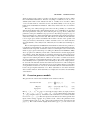
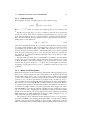
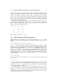
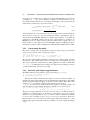
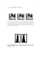
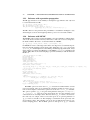
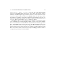
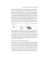
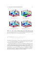
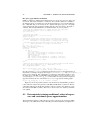
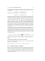
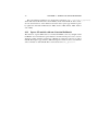
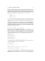
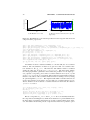
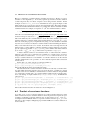
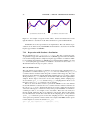
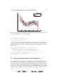
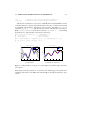
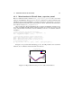
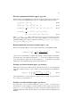
Figure 7.4: GP solutions (a MAP estimate) with squared exponential covariance function and binomial likelihood in a toy example.
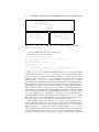
% Set the approximate inference method
gp = gp_set(gp, ’latent_method’, ’Laplace’);
gp=gp_optim(gp,x,y,’z’,N,’opt’,opt);
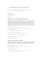
To make predictions with binomial likelihood model without computing the predictive density, the total number of trials Nt in test points needs to be provided (in
addition to N that is total number of trials in training points). In GPstuff, this is done
as following:
% Set the total number of trials Nt at the grid points xgrid
[Eft_la, Varft_la, Eyt_la, Varyt_la] = ...
gp_pred(gp, x, y, xgrid, ’z’, N, ’zt’, Ntgrid);
To compute the predictive densities with binomial likelihood...
% To compute predictive densities at the test points xt, the total number
% of trials Nt must be set additionally:
[Eft_la, Varft_la, Eyt_la, Varyt_la, pyt_la] = gp_pred(gp, x, y, xt, ’z’,
N, ’yt’, yt, ’zt’, Nt);
7.5
Derivative observations in GP regression
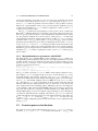
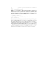
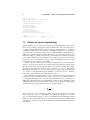
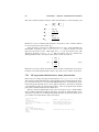
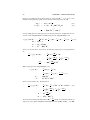
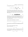
Incorporating derivative observations in GP regression is fairly straightforward, because a derivative of Gaussian process is a Gaussian process. In short, derivative observation are taken into account by extending covariance matrices to include derivative
observations. This is done by forming joint covariance matrices of function values
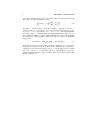
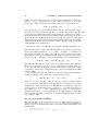
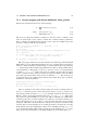
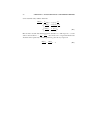
and derivatives. Following equations (Rasmussen and Williams, 2006) state how the
covariances between function values and derivatives, and between derivatives are calculated
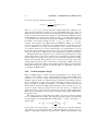
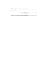
Cov(fi ,
∂k(xi , xj
∂fj
)=
),
∂xdj
∂xdj
Cov(
∂fi ∂fj
∂ 2 k(xi , xj
,
)=
.
∂xdi ∂xej
∂xdi ∂xej