1
Dislocation Dynamics User’s Manual
Generated by Doxygen 1.5.8
Tue Sep 28 14:01:25 2010
CONTENTS
1
Contents
1 User’s manual for dislocation dynamics simulation
1
2 Installation
1
2.1
Getting the code . . . . . . . . . . . . . . . . . . . . . . . . . . . . . . . . . . . . . . . .
2
2.2
Compiling . . . . . . . . . . . . . . . . . . . . . . . . . . . . . . . . . . . . . . . . . . .
2
2.3
Libraries . . . . . . . . . . . . . . . . . . . . . . . . . . . . . . . . . . . . . . . . . . . .
2
2.4
Installation . . . . . . . . . . . . . . . . . . . . . . . . . . . . . . . . . . . . . . . . . .
3
3 Output
3
3.1
Thermodynamic variables . . . . . . . . . . . . . . . . . . . . . . . . . . . . . . . . . . .
3
3.2
Saving and loading state . . . . . . . . . . . . . . . . . . . . . . . . . . . . . . . . . . .
3
3.3
Dislocation screen . . . . . . . . . . . . . . . . . . . . . . . . . . . . . . . . . . . . . . .
4
3.4
Video output . . . . . . . . . . . . . . . . . . . . . . . . . . . . . . . . . . . . . . . . . .
4
3.5
Time-activity plots . . . . . . . . . . . . . . . . . . . . . . . . . . . . . . . . . . . . . .
4
3.6
Animation . . . . . . . . . . . . . . . . . . . . . . . . . . . . . . . . . . . . . . . . . . .
4
4 Running the simulation
5
4.1
Displaying help . . . . . . . . . . . . . . . . . . . . . . . . . . . . . . . . . . . . . . . .
5
4.2
Example 1: Analyzing drift strainrate . . . . . . . . . . . . . . . . . . . . . . . . . . . .
5
4.3
Example 2: Studying the PLC effect . . . . . . . . . . . . . . . . . . . . . . . . . . . . .
7
4.4
Saving and loading state . . . . . . . . . . . . . . . . . . . . . . . . . . . . . . . . . . .
9
4.5
Examples of specifying parameters . . . . . . . . . . . . . . . . . . . . . . . . . . . . . .
9
5 The code and algorithms
10
5.1
Efficiency of algorithms . . . . . . . . . . . . . . . . . . . . . . . . . . . . . . . . . . . .
11
5.2
A few thoughts on C++ for numerical physics . . . . . . . . . . . . . . . . . . . . . . . .
11
1 User’s manual for dislocation dynamics simulation
This document tells how to operate the simulation and how to use the provided tools to analyze the output.
For explanation of the physics and algorithms, see the scientific document that comes with this program.
The HTML documentation available at ./html/index.html of the package comes with a full class and files
reference manual.
2 Installation
Generated on Tue Sep 28 14:01:25 2010 by Doxygen
2.1
2.1
Getting the code
2
Getting the code
The code can be obtained with GIT:
git clone git://tuomastonteri.fi/ddsim
2.2
Compiling
Type "make" (or "./scons") at the root directory.
Compiling needs python >= 1.5.2. Available libraries will be detected automatically by Scons. For
additional parameters try "./scons –help". For more information look at the Sconstruct python file and the
following examples:
• "scons ddmain" will only build program ddmain
• "scons –config=force" will recheck library and header dependencies
• "scons –clean" will clean all targets
Has been tested to compile on several unix/linux systems including:
• melkinpaasi.cs.helsinki.fi (27.1.2010)
• ruuvi.helsinki.fi (27.1.2010)
• punk.it.helsinki.fi (27.1.2010)
Does not compile on :
• kruuna.helsinki.fi (27.1.2010) lacks required Boost libraries
2.3
Libraries
Required:
• Boost Thread for multithreading
• Boost Random for random number generation
• Boost Program_options for command line parsing
These are found in most Linux distributions, including the one used by HUT Fyslab kvartsi and desktop
computers.
Additional:
• Compiler OpenMP support for multithreading
• SDL for visualization and image saving
Generated on Tue Sep 28 14:01:25 2010 by Doxygen
2.4
Installation
3
• ffmpeg for animation video output
• Boost Serialization for saving/loading simulation state
• Boost Iostreams for compressing and decompressing data files. Version greater or equal to
1.34.
• Boost Filesystem for platform independent directory access
2.4
Installation
Scons will create the following executables at ./bin/ directory:
• ddmain , the simulation. See Output and Running the simulation
• activ , See activ.cpp and examples at Running the simulation
• play , See play.cpp and examples at Running the simulation
• dataplot , dataplot.cpp and examples at Running the simulation
3 Output
The output of the simulation is mostly designed for the study of the PLC effect. For this particular usage it
is necessary to see the full ’simulation history’ and not just a few thermodynamic variables as a function of
time. This makes it necessary to use binary format and compression at places to avoid too large datafiles.
3.1
Thermodynamic variables
The simulation outputs the following thermodynamic variables:
• Average strainrate of dislocations as a function of time
• Average velocity of dislocations as a function of time
• External force as a function of time
• External force as a function of accumulated strain (what is measured experimentally)
3.2
Saving and loading state
After completion or termination the simulation will output a statefile into the data directory, which holds
the full state of the simulation. One can load back that particular simulation state and continue it from any
computer. For using this see the help (–help) of the main executable.
The purpose of this feature is to be able to continue analyzing interesting scenarios run on computing
clusters. It can also be used to stop the simulation and change parameters on the fly to eg. prepare the
material in a certain way. Also useful in case of a scheduled reboot of a cluster, where the program can
output its state after receiving the unix terminate signal.
Generated on Tue Sep 28 14:01:25 2010 by Doxygen
3.3
3.3
Dislocation screen
4
Dislocation screen
• Visualizes the dislocations, solute-atoms and pinning centers in realtime on monitor
• Enabled with "-X" or "–display"
For debugging and analyzing the effect of changing input parameters
It supports mouse and key operation:
• Pause with key SPACE.
• Zoom by holding the left mouse button and dragging to choose a section. Right or middle button
will reset the zoom.
3.4
Video output
• Outputs the dislocation screen to a videofile in datadirectory in .avi MPEG4 format (play with
mplayer)
• Enabled with "dd -V" or "dd –video"
For saving animations of full simulations
3.5
Time-activity plots
• Outputs the strainrate of each individual Dislocation row as a function of time in custom binary
format (move.dat)
• Disabled with "dd -I" or "dd –noactivity"
The purpose is to get quick overall picture on if the PLC band propagation is taking place. This would
show as either correlated localized bursts of activity or random localized bursts of activity.
The data can be converted into a .bmp image and viewed with the additional tool "activ". See activ.cpp
3.6
Animation
• Outputs Dislocation animation in custom binary format, that can be viewed with tool "play". See
play.cpp
• Outputs to (anim.dat)
For saving animations of full simulations
Output possible only when the number of dislocations equal the simulation y-size. Gives small filesize for
accurate animation of the Dislocations. If Solutes and PinningCentres need to be visualized one must use
the video output instead.
For usage examples see Running the simulation
Generated on Tue Sep 28 14:01:25 2010 by Doxygen
4 Running the simulation
5
4 Running the simulation
The code has been designed so that each feature builds on the existing code rather than replacing it or
’forking’ by copying to a new project and altering it. This means that each new feature also needs a new
command line parameter. All possible combinations of sane parameters should be valid.
4.1
Displaying help
To see the available parameters and their default values:
ddmain --help
4.2
Example 1: Analyzing drift strainrate
The simulation has been used to study the stable ’drift’ strainrate of a dislocation system when a relatively
small constant external force is applied. In this situation the drift strainrate as a function of external force
shows a certain kind of characteristic behaviour. This provided, that the applied force is just in the right
range, not too small and not too large. Too small might show zero drift and too large will ’tear’. A
behaviour in line with experiments with real materials might tell something about the dynamics of this drift
behaviour.
To do this one can use the rundd.py helper script to run a simulation with varying external force in some
range (a BASH script would fail to provide floating point increments):
./rundd.py 100 1000 100 -x 50 -y 50 -N 50 --timemax 0.075 --fps=1
In this particular case the force is from ’100’ to ’1000’ with a step size of ’100’. This particular range was
determined after first running the simulation with the dislocation screen on and observing where roughly
the behaviour ’tears’. Also the simulation time (0.075) was determined in the same way by observing when
a somewhat steady state has been reached in these systems by looking at the (time,strainrate) plot. The –fps
parameter just specifies how often the time is printed in secounds in console (or how often the graphical
display is updated when switched on). Note that on average desktop the above command will take at least
30 minutes to complete. The dataplot utility can be used to visualize whether a steady drift rates really had
been reached:
./dataplot --dataname=strainrate
In this case an example data is provided at ./bin/datasteady/ . It can be viewed with:
./dataplot --datadir=./datasteady/ --dataname=strainrate
The example data has been sampled 10 times (repeats of the above rundd.py command line) and gave the
following result (a few of the velocities were ran to 0.125 instead of 0.075):
Generated on Tue Sep 28 14:01:25 2010 by Doxygen
4.2
Example 1: Analyzing drift strainrate
6
The strainrate is reasonably stable at 0.075, but it would have been somewhat better to run all to 0.125.
Next the dataplot utility can be used to plot stready strainrate as a function of driving force as follows:
./dataplot --datadir=./datasteady/ --dataname=strainrate --function=d --s_use=0
The above command causes the program to ignore the seed as unique data identifier so an average is taken
of these datapoints. It plots strainrate as a function of parameter ’d’ or in this case force. In this case the
average is taken of the last 500 points of each data to determine the steady drift rate. The result is as follows
after renaming a few lines in the resulting: gnuplot.macro:
Generated on Tue Sep 28 14:01:25 2010 by Doxygen
4.3
Example 2: Studying the PLC effect
7
The sampling is still rough, but indicates a fast growth starting at about 500 and a possibly a different kind
of behaviour from zero to 500 (the drift behaviour). It might be desirable to analyze the range 0-500 in
more detail with a somewhat larger than a 50x50 system.
• rundd.py is a helper script, which runs dd with varying external drives specified by minimun value,
a maximun value and a step size
4.3
Example 2: Studying the PLC effect
The default values in the simulation for all the numerous parameters have been selected to be somewhat
sensible for this use (more about that in the accompanying scientific document). One needs to enable
constant strainrate drive and several optional outputs:
./ddmain --constdrive -A1 -V -X -z 7
This enables constant strainrate drive, animation, video, display and enlarges display by 7x. Running this
with the default parameters until about t=1.0 can result in the following configuration:
Generated on Tue Sep 28 14:01:25 2010 by Doxygen
4.3
Example 2: Studying the PLC effect
8
The red and blue things are dislocations, green dots are solute atoms and the white is background. Note
some artifacts in the diffusing solute clouds. These are due to an optimization whereby solutes too far away
from any dislocations are not moved at all. To quickly see what dislocations have moved one can use the
activity tool:
./activ ./data/move.[...].dat.gz
Which results in the following output:
The white areas are rows with the most activity and the darker it gets the less movement there was. This
shows that certain groups of dislocations are frozen by the solute atoms while the others move constantly.
The same can be seen from video and animation outputs:
./play ./data/anim.[...].dat.gz
mplayer ./data/video.[...].avi
More information about this use can be found at the scientific document.
Generated on Tue Sep 28 14:01:25 2010 by Doxygen
4.4
4.4
Saving and loading state
9
Saving and loading state
By default a state file is written into the datadirectory when a simulation is terminated. This can be loaded
for examination with the following command:
./ddmain --stateload ./data/state.[..].dat.gz
Note that the display, zoom and video has to be specified again if those outputs are desired. To actually
continue writing any data additional option ’statecontinue’ is needed:
./ddmain --stateload ./data/state.[..].dat.gz --statecontinue
The data writing will append into the existing thermodynamic output. Video files, animation files, activity
and state file will be overwritten.
There are also some parameters to override options when continuing states such as ’newmaxtime’. These
are stated under "State write options" in the main executable help. More can be added on need basis into
the source without breaking existing state files.
4.5
Examples of specifying parameters
To run a simulation with just dislocations and a constant driving force, with screen enabled:
ddmain -d 0.1 -X
Just dislocations and with a constant strainrate drive:
ddmain -p -d 0.1
Adding relaxation time of 5000 time units:
ddmain -p -d 0.1 -R 5000
Just dislocations, constant strainrate drive and strain hardening:
ddmain -p -d 0.1 -H
Adding solute-atoms:
ddmain -S 1.0 -T_S 0.01
where S is the relative amount of sim area and T_S is the temperature (not in K)
Enabling video output:
ddmain --video
For further usage see the sections in "–help"
Generated on Tue Sep 28 14:01:25 2010 by Doxygen
5 The code and algorithms
10
5 The code and algorithms
I was given some C code in 2007 involving dislocation to dislocation interaction. The current code is
completely my own, modified in structure for this programming exercise from a C/C++ hybrid it was back
then then to a full object oriented design. Also documentation including this manual has been improved
considerably.
This project has been coded with C++ using a modular (object oriented) design and principles of generic
programming. The latter means to implement a functionality only once in as general way as possible, do it
properly, and then use that implementation in different sorts of situations. For example, the Runge Kutta
algorithm can be easily utilized in other programs and also it would not be too hard to swap in a different
numerical intergration algorithm. The same is true for the Datawrite class and many other components,
which have been designed for general simulation use.
The classes of the project and their dependencies are illustrated in the following figure, where an arrow
head points to a dependency (the graph is constructed from a hand made description and might not be
100% accurate):
Of course, entities such as a dislocation, solute and a pinning center make up a class. For example in a
Dislocation class there is all the related data such as the position and accumulated strain. Additionally there
is constructor to create a dislocation and public member functions to calculate forces between a dislocation
and other entitities and to call the numerical integration algorithm to solve the next position.
Next there are the classes Dislocations, Solutes and PinningCenters. Everything related to, for example,
dislocations collectively is here. This includes the data, which is all the dislocations in a linked list. Also
this includes public members functions to create all dislocations, solve forces between all the dislocations
and all the other entities and also to numerically integrate the dynamics.
Generated on Tue Sep 28 14:01:25 2010 by Doxygen
5.1
Efficiency of algorithms
11
Having all the above mentioned functionality implemented, all that is left from running a simulation is to
initialize the Dislocations, Solutes and PinningCenters classes. This happens at Ddsim class. In its constructor everything is initialized and in its public member function MainLoop() the simulation is iterated.
Ddsim also uses the different output classes to output data as can be seen from the figure above.
The Runge Kutta algorithm has been implemented as a template class in class RungeKutta2, where the
number of dimensions can be specified as a template parameter. A Dislocation is a child class of it with
one dimensional dynamics. A Solute is the same with two dimensions.
Finally, random numbers are provided by the Ranfac class. Its public member functions are thread safe
and it uses one generator for each thread transparently to the user with OpenMP. The class itself is static
(initialized at the beginning on main() automatically) and gets its own seed and so it can be used without
any initialization. Of course, also a custom seed can be provided.
The public interfaces of all the Classes are documented in the Classes and Files section of this manual and
also the full source can be browsed.
5.1
Efficiency of algorithms
This part gives an overall summary of the algorithms used from the point of view of computational efficiency.
The dislocations are stored in a linked list, because this allows easy removal in case many dislocations
get annihilated. This didn’t benchmark any meaningful difference to a linear array. The forces between
dislocations are solved by calculating the force from the first to the rest (and at the same time in the opposite
direction, which is just negative from the other direction). Then from the secound to the rest, except the
first, and so on. This leads to (N-1)+(N-2)+(N-3)+ .. + (N-N) iterations. This is exactly N(N-1) - N(N-1)/2
iterations or O(N²/2 - N/2). There is no getting around this with 1/r force.
All the solute atom data is stored in an array, because the amount is kept constant. Additionally the
simulation area is divided into fixed sized blocks in the amount of X times Y (so 100² for 100∗100).
These blocks are stored in an array, where each member is a linked list of pointers to solute atom data.
Now, the force between dislocations and solutes is only solved from solutes that are certain blocks away
from the dislocation in a rectangle. This is also a runtime parameter. Additionally an array of booleans is
kept updated, which say in which blocks solutes interacted with any dislocations the last iteration. Those
solutes that weren’t in blocks that interacted are not updated or touched except to zero forces each iteration.
These allow to have a huge number of solute atoms especially if most of them are in blocks that do not
interact with dislocations. Just zeroing the force memory in the array of solutes is extremely cache optimal
operation.
In this version of the code only the dislocation <-> dislocation interaction is parallelized using
Boost::threads or a modification of it called threadpool. This is just a proof of concept. The implementation
is not particularly elegant unlike OpenMP, but very efficient. With two core CPU the performance increase
can near 95-99% with very large dislocation systems depending on the percentage of total run time spent
calculating the dislocation force function.
In principle, a new OpenMP 3.0 concept of tasks should allow to parallelize object oriented code in extremely nice fashion. Also 3.0 brings support for C++ iterators. In practice, all compilers tried failed at the
start of the year 2010 to produce efficient parallel code with either features. This is what I would like to
use to parallelize this project (mainly solute <-> dislocation interaction).
More details about the efficiency of the code is found in the source directory.
5.2
A few thoughts on C++ for numerical physics
Good:
Generated on Tue Sep 28 14:01:25 2010 by Doxygen
5.2
A few thoughts on C++ for numerical physics
12
• Much, much faster to code than C (mainly due to C++ standard libraries)
• Encourages the usage of standard libraries and methods instead of creating buggy ad hoc C solutions
• Clearer, more generic and expandable code when little time is spent designing the class structure
• Just as fast in executing time when properly used than any C implementation
Bad:
• Code complexity is considerably higher than in C. Especially template rich C++ looks nasty. However, advanced concept can be avoided when introducing to C++.
• Can be slow to compile
Generated on Tue Sep 28 14:01:25 2010 by Doxygen