1
User Guide for ARTS
System-on-Chip Group
Technical University of Denmark
1. INTRODUCTION
This document is targeted for the users of the system-level multiprocessor system-on-chip
(MPSoC) simulation framework, called ARTS, developed at the Technical University of
Denmark (DTU). The framework allows to:
· model processing elements (PE), memory units and interconnect,
· investigate PE utilization, memory usage, communication issues, and energy/power consumption, and
· analyze the causality between MPSoC components i.e. resource constrains and interdependencies
This document explains the various aspects relating to the use of the SystemC [SystemC
2002] implementation of the ARTS framework. The latest version of the framework can
be found at:
☛ http://www.imm.dtu.dk/arts
Before proceeding further, we explain some of the conventions used in this document.
The symbol ☛ marks an important information. Text presented in a box mark user action
such as entry at the command prompt. Further we assume the operating environment to be
linux-like platform.
This document is organized as follows. First, in Section 2, some details about the ARTS
executable is provided. This is followed by the description of the inputs expected by this
executable (Section 3). A successful simulation of the given problem, results in a collection
of files for analysis, which are explained in Section 4. Finally a brief, Section 5 walks the
reader through using the ARTS model.
2. THE EXECUTABLE AND SUPPORT FILES
Depending on the platform choose, the executable is named: arts_<platform>.x.
In a unique folder, download the version best suited to your conditions. Along with the
executable, a support_files.tar.gz should also be acquired and saved in the same
location as the executable. The files within this bundle are used in the running example
within the document and are necessary to complete the tutorial. The first test is simply to
issue the command to run the executable.
$> ./arts_<platform>.x
Figure 1 should be the outcome. It implies that additional arguments are needed to be set,
Document version: 1.0. Drafted on September 2005.
Address: Technical University of Denmark, Informatics and Mathematical Modelling, Richard Petersens Plads,
Building 321, DK-2800 Lyngby, Denmark. Contact email: Shankar Mahadevan ([email protected])
© 2005 Technical University of Denmark
2
·
Technical Uinversity of Denmark
===============================================================
ARTS SoC Modelling Framework
Copyright (C) 2005 Department of Informatics and Mathematical Modelling, DTU
===============================================================
Please check the arguments to the executable:
./arts_<platform>.x -app <path>/<filename>.tg <path>/<filename>.tg
-rsc <path>/<filename>.rsc <path>/<filename>.rsc
-cmm <path>/<filename>.cmm
-prt <path>/<filename>.prt
<ocpConfig_file>
<num of PE>
exectime
Fig. 1. Arguments required with the ARTS executable.
Argument Flag
-app
Arguments
1 or more .tg files
-rsc
-cmm
-prt
1 or more .rsc files
1 or more .cmm files
only 1 .prt file
<ocpConfig_file>
<num_of_PE>
execttime
only 1 file
0 to ∞
0 to ∞
Comments
this takes one or more file(s) describing the applications
task graphs
this takes one or more file(s) describing the PE characteristics
this takes the communication description
this takes one file that describes the architecture i.e. PE with
the interconnect, and the mapping of the tasks on to the PEs
this is one file describing the OCP signal configuration
the number of PEs in the architecture
the cycles to be simulated
Table I. Expected arguments for the ARTS executable.
to operate the executable. Note any other outcome implies an incompatibility between the
executable and the underlying platform. The source code of the ARTS framework would
need to be compiled on this platform to proceed further. The arguments of the executable
and their meaning is explained in Table I. The five primary items: the application, PE,
communication, and architecture/mapping and OCP configuration file will be discussed in
detail in the next section. The remaining items related to prescribing the number of PE in
the architecture and the number of cycles to simulate.
Unpacking the support files bundle will provide the necessary argument files for demonstration of the ARTS framework. Figure 2 is one of the simple possible complete command
to run the simulation. The similarity of argument fields in this command, and in Table I and
Figure 1 are obvious. A successful simulation will have the Simulation end time
(last few lines in display) equal to given number of cycles to simulate, followed by simulation time statistics. The output of a successful simulation is also a collection of log files.
Before we explain the contents of the output files, as done in Section 4, let us take a closer
look at the input argument files.
3. UNDERSTANDING THE INPUTS
The primary inputs to the ARTS framework are ASCII files describing the application
model (.tg extension), the PE characteristics (.rsc extension), the communication properties
(.cmm extension) and the architecture with the application tasks mapping (.prt extension).
First, we provide a brief overview of the application, PE and communication files. For
additional details on these files, we the refer the reader to [Schmitz et al. 2004]. Then,
·
User Guide for ARTS
3
$> ./arts_<platform>.x
-app ./support_files/apps/sample1.tg ./support_files/apps/sample2.tg
-rsc ./support_files/rsc/GPP0.rsc ./support_files/rsc/ASIC0.rsc
-cmm ./support_files/cmm/COMM.rsc
-prt ./support_files/prt/sample.prt
./support_files/ocp
2
30000
Fig. 2. Sample Simulation Command
# THIS IS SAMPLE TASK GRAPH !
HYPERPERIOD 0.025
TOLERABLE_TIMING_PENALTY 1.0 # 1.2 is 20% variation
# in execution time
τ0
τ1
τ2
τ3
τ4
Task:
Task:
Task:
Task:
Task:
(00)
(01)
(02)
(03)
(04)
ttype:
ttype:
ttype:
ttype:
ttype:
Edge:
Edge:
Edge:
Edge:
Edge:
(00)
(01)
(01)
(02)
(03)
–>
–>
–>
–>
–>
4
2
3
3
0
epst:
epst:
epst:
epst:
epst:
(01)
(02)
(03)
(04)
(04)
0
0
0
0
0
dtype:
dtype:
dtype:
dtype:
dtype:
etype:
etype:
etype:
etype:
etype:
NON
NON
NON
NON
NON
Deadline:
Deadline:
Deadline:
Deadline:
Deadline:
0
0
0
0
0.025
2
2
4
1
0
Fig. 3. Sample Task Graph
Fig. 4. File description of a task graph (.tg file), say sample.tg.
we describe our architecture description and application task mapping file. Table 21 in
Appendix A spells out the meanings of the labels used in these files.
3.1 Application (.tg) Characterizations
We consider the applications to be modelled as a task graph G = (T , E), where T = {τi :
1 ≤ i ≤ n} is the set of schedulable tasks, and E = {ej : 1 ≤ j ≤ k} is the set of directed
edges representing the data dependencies (precedence constraints) between the tasks in T ,
i.e., if τi ≺ τj then (τi , τj ) ∈ E. Figure 3 shows a sample task graph with five tasks and five
edges. The weight of an edge indicates the size of the message to be transferred between
two tasks. Each task τi ∈ T is characterized by a four tuple hdi , ti , ci , ei i, i.e. the exact
functionality of the task is abstracted away. The relative deadline, di , and the period, ti , are
given by external requirements of the application and, hence, are independent of runtime
input values, intermediate results or configurations of PE cores. However, the execution
time, ci , and the consumed energy, ei , are both determined by the actual mapping of the
task onto a particular PE.
The deadline of a real-time application, DT , is represented by the deadline of the task(s)
in T with no successors, i.e. no outgoing edges. The concurrent execution of several realtime applications, each with their own deadline and period, is handle as a set of task graphs
which have to be mapped onto the platform architecture.
Figure 4 is the file description, a .tg file, of the sample task graph shown in Figure 3.
Lines starting with # are comments, which continue until the end of the line. The period
4
·
Technical Uinversity of Denmark
# THIS IS THE TECHNOLOGY FILE
@GPP 0 {
# Price
StPwr
100
800
# ttype
0
1
2
3
4
..
..
}
Version
0
0
0
0
0
Freq
25000
CommBuffer
1
CommTime
0.271247
CommPower
2000
CommMem
13
ExeCyc
2882
200
100
981
395
DynPwr
25000
25000
25000
25000
25000
StMem
400
400
400
400
400
DynMem
400
400
400
400
400
Preem
1
1
1
1
1
Exable
1
1
1
1
1
Fig. 5. File description of PE (.rsc file).
and the deadline, the PE-independent tuples, can be easily recognized via the values of
HYPERPERIOD and by looking at the end task, respectively. The values are given in
seconds, which for this sample task graph is identical and equal to 0.025 s. With regards to
variations in the execution time, ci , in order to calculate the worst-case execution time we
use the value of keyword TOLERABLE_TIMING_PENALTY. In this case, Figure 3, the
worst-case execution characteristics is expected to be same. Within the file, the task graph
is described via task description and edge description separately, in that order.
In Figure 4, each line starting with Task: uniquely identifies a task within the task
graph. In addition to task identifier, the bracketed item, each task has a task type (ttype).
The task type is used to apply the PE-specific tuples such as execution time and energy
consumption, when bounding this task to a particular PE. This affords flexibility during
instantiation as changing the underlying PE does not need manipulation of the application
files, but simply applying the new values of this task type from the PE database. This will
be described in additional detail in the next section. In addition to the four tuples, two
additional variables epst: (earliest possible start time) and dtype: (deadline type, i.e.
NON, SOFT, and HARD) are also available for future use. The default value, accepted by
the current version of the ARTS framework is displayed in the figure.
Each line starting with Edge: uniquely identifies an edge between two task, and the direction of their interdependency, within the task graph. One task may have many outgoing
and incoming edges, but each edge needs to be identified separately. Similar to task type,
edge type (etype) is used to apply the message transfer characteristics depending on the
particular communication means.
3.2 PE (.rsc) files
ARTS supports many PE types. The built-in PEs are general purpose processors (GPP),
FPGAs and ASICs. A sample PE description of GPP is shown in Figure 5.
The IP type of the PE is given by line starting with @. Each file should have unique
IP type. Multiple PE of the same type can be tagged with additional numeric value, for
example @GPP 0, as shown in the figure. The PE properties are encapsulated in opening
and closing brackets ({ and }). Within the file, first the task-independent properties are
described, followed by the task properties.
User Guide for ARTS
·
5
@COMM_AMOUNT 0 {
# etype
comamount
0
16
1
330
2
320
3
36
4
16
}
Fig. 6. A Sample Communication description in .cmm file.
The PE’s task-independent properties are listed as items starting with price, static power
(StPwr), operating frequency (freq), etc. The PE’s task properties include number of
clock cycles required for execution (ExeCyc), dynamic power dissipation (DynPwr),
memory requirements, etc. In addition to these properties, other ASIC and FGPA related
items such as area and CLBs, respectively, required to implement the task is also available
(See Table 21 in Appendix A. Also ASIC0.rsc file in support_file/rsc).
The PE’s task properties are listed next. When a task from the task graphs is mapped
to a particular PE, the task properties can be extracted by looking up the index of the
ttype in the .tg file and matching it with the task type in .rsc file. Correlating the data
given in Figure 4 and Figure 5, it is seen, for example, that task (0 1) in the task graph
requires 100 cycles for execution in GPP0, and so on. The ARTS framework, automatically
correlates these values, using the architecture and the mapping described in the .prt file,
which is discussed later.
3.3 Interconnect (.cmm) files
Within ARTS, the message size is described in the .cmm file. Similar to .rsc files the
communication properties is described within closing brackets ({ and }). By correlation
between the etype described in the task graph, with the appropriated index, the message
size to be transferred for a given edge can be calculate. Correlating the data given in
Figure 4 and Figure 6, it is seen, for example, that the edge between the task (0 1) and
(0 3) requires the 16 words of data units.
Using these three files, the MPSoC designer can influence the properties of the application, PE and communication for any architecture instantiated within the ARTS framework.
The designer is not limited to the built-in templates. Any application, PE or communication data conforming to the file semantics can be used as inputs to instantiate a custom
platform.
3.4 Architecture (.prt) files
The architecture file describes the MPSoC modules such as the PEs and the interconnect,
and the mapping of the task from the task graph on to these PEs. In addition to this primary
purpose, the file also contains the frameworks simulation controls such as display of debug
messages and monitoring system parameters. Figure 7 shows a sample architecture file.
The file can be distinguished into five parts.
The first two parts, which are optional, relate to enabling simulations items such as
dumping the PE, application or communication events on the screen, or capturing these
values in a file. Additional parameters PE utilization, communication and/or memory pro-
6
·
Technical Uinversity of Denmark
# — On-screen Simulator debug message (0=off, 1=on)
pe_screen_dump
=0
# dump PE events
soc_screen_dump
=0
# dump communication events
# — Enable output logging via files (provide unique filename, no spaces)
app_logfile
= "app.log"
# stores application events
pe_logfile
= "pe.log"
# stores PE utilization
result_file
= "result.log"
# stores architecture overview
memory_file
= "mem.log"
# stores memory profile
contention_file
= "comm.log"
# stores communication profile
vcd_file
= "sim"
# default extension .vcd
# Communication description
module {
# — Communication topology (0=bus, 1=mesh)
soc_comm_topology
# communication keyword
soc_allocator
=0
# bus
}
# PE description
module {
# — configuration for PE#0
peID
=0
# unique processor identifier
address
= 0x0000000:0x0fffffc
processor
=0
# processor type, see rsc argument
synchronizer
=0
# synchronizer type
resource_allocator
=0
# allocator type
scheduler
=0
# scheduler type
monitor
=0
# specific PE debug msg dump
PE#0
}
module {
# — configuration for PE#1
peID
=1
PE#1
address
= 0x1000000:0x1fffffc
processor
=1
# match index with rsc argument
synchronizer
=0
# 0=direct synchronization
resource_allocator
=0
# 0=basic priority inheritance
Fig. 8. Sample Architecture
scheduler
=0
# 0=RM, 1=EDF
monitor
=0
# 0=off, 1=on
}
# Mapping of task from .tg files to PE
application {
# <taskID>,<peID> mapping
name: "sample.tg"
# identify using .tg filename
task:
1, 0
# task (0 0) mapped to PE#0
task:
2, 1
# task (0 1) mapped to PE#1
task:
3, 0
# .. so on.
task:
4, 1
task:
5, 0
}
application {
name: "sample2.tg"
# another sample application
task:
1, 0
task:
2, 1
task:
3, 0
task:
4, 1
task:
5, 1
task:
6, 1
}
Fig. 7. A Sample Architecture description in .prt file.
User Guide for ARTS
·
7
file can also be captured in spreadsheet-friendly format via providing a filename to the
appropriated keywords (no space within the filenames). These files are explained in next
section. To disable logging of any specific event, simply comment out the appropriate
keyword. This may led to smaller simulation time as well.
The next two part describe the architecture, where each component is described at
module. The module descriptions starts with the interconnect, which is identified by
keyword soc_comm_topology as the communication module. The topology is identified by another keyword soc_allocator, which takes a numeric value identifying bus
or multi-hop network interconnect. The remaining module characterize the PE that use this
interconnect.
In the case of Figure 7, we have two PEs, each identified by a unique ID
(peID) and memory space (address). Following these declaration, are five parameters: processor, synchronizer, resource_allocator, scheduler, and
monitor; that are used to assign execution and OS characteristics to this PE. The
processor can have values equal to the index of the rsc argument (see Table I). Comparing the architecture file in Figure 7 and the sample simulation command in Figure 2,
for this example: PE#0 is of type GPP0 and PE#1 is of type ASIC0. This allows easy
replacement of the PE execution characteristics: either via the architecture file or at the
command line. The final keyword, monitor, can be used to display the PE’s events
on the screen when the primary simulation pe_screen_dump is off, thereby allowing
monitoring/debugging of individual PE activities.
The synchronizer, resource_allocator, and scheduler keywords take
numeric index of corresponding built-in ARTS synchronizer, resource allocator and scheduler, respectively. Within the ARTS, the user can apply Direct Synchronization (index
0) for the task synchronization, basic priority inheritance (index 0) for the resource allocation, and Rate Monotonic (RM) (index 0) and Earlier Deadline First (EDF) (index 1)
for the task scheduling. Additional built-in OS components can be coded easily using the
available features in the source code, however are currently unavailable with the ARTS
binary.
Together, all module descriptions, enable visualizing the architecture. figure 8 represent
the architecture described in Figure 7. Any number of modules can be instantiated to realize a custom architecture. The final part of the architecture file is the application mapping
i.e. prescribing which tasks are mapped to which modules. Mapping has to be described
for each application separately and it is done within the application group (enclosed
within { and }).
The application can be identified using the name, which should have a corresponding
filename associated with the app argument (see Table I) of the executable. Further, the
number of tasks defined in the application block should match the number of tasks in
the prescribed application task graph file (.tg file). To begin mapping, each line has to start
with keyword task: followed by the pairing of the task index and the PE index i.e. the
peID.
☛ Note the task index have to be offset by one. This is legacy code requirements and
will be fixed in future versions of the ARTS release.
In our running example, comparing the Figures 4, Figure 7 and Figure 8, for the sample
application (filename: sample.tg) the tasks are alternately mapped to PE#0 and PE#1. As
seen for sample2.tg application, any mapping can be applied. In all, there are 11 tasks, 5
8
·
Profile
0
Technical Uinversity of Denmark
Task Count
11
PE0
GPP0
PE1
ASIC0
ET@app0
14931 us
Deadline
MET
ET@app1
20694 us
Deadline
MET
Total ET
20694 us
Fig. 9. Architecture Overview file.
tasks are mapped to PE#0 (GPP0) and 6 tasks are mapped to PE#1 (ASIC0).
In addition to above three types of files, an OCP signal configuration files [OCPIP 2004]
is required with the input arguments. It contains the OCP signals and their values used at
the PE interface with the interconnect and follows the standard format available with OCP
channel package described in related manual available from OCP website.
Any error, for example: incorrect spelling, syntax errors, incorrect string and index
values, reuse of unique keywords or values, mismatch between command string input and
values, etc; are flagged during parsing of the input files and the simulation terminates
immediately with appropriate message. Upon correct parsing of all the related inputs, the
simulation can be successfully initiated by the ARTS framework. As previously discussed
in Section 1, the support_files.tar.gz contains a sample of these input files for
real application and PEs, and the command presented in Figure 2 can be used to execute
the ARTS model. The output resulting from this and similar execution is discussed next.
4. UNDERSTANDING THE OUTPUTS
Based on which events are enabled for recording (Figure 7) multiple spread-friendly files
are generated that provide an overview of the architecture-under-test, and the profile of the
application, the PE utilization, the memory or the communication. Consider the outputs
for the simulation executed by command in Figure 2. The outputs file are illustrated in
Figures 9 to Figure 14.
For the architecture overview and the PE utilization files, each column has a single
data item. Profile is the architecture identifier used internally in ARTS to tag different
architectures. Here since, we only have one architecture for exploration the value is 0.
The architecture overview file, Figure 9, can be used to confirm the inputs, such as task
count and PE types. Additional data pertains to the completion time (end time (ET)) and
the deadline status (MET or MISS) of individual applications is also provided here. The
final two columns Total ET and Contention, provide the final completion time of
the program (which should be equal to the application that finished last) and the interconnect contention count i.e. the count conflicting concurrent link access over the program
execution. If the values in this file are satisfactory, further analysis of the rest of the output
files may be undertaken.
☛ The ET of the application, is the completion time of the last invocation of the application. In the case, where the provided number of cycles of simulation (execttime
argument) is significantly larger than anticipated program completion time or the period
of the applications, the applications will be invoked multiple times and the completion
time of the final invocation is recorded in the overview file.
☛ In the case that the provided number of cycles to simulate (execttime argument) is
insufficient to finish program execution, 0 s is displayed for ET.
Contention
0
User Guide for ARTS
PE Utilization:
Profile
PEU0
0
75.6467
PEU1
23.8467
Fig. 10. PE Utilization file
Communication Profile:
Time
Contention
1
0
1749
4
..
..
12834
1
16049
0
Fig. 12. Dummy Communication Profile
·
9
Application Profile: Platform Architecture 0
14931 ns Task graph sample1.tg (AppID 0) completed.
20694 ns Task graph sample2.tg (AppID 1) completed.
Fig. 11. Application Profile file.
Memory Profile: Platform Architecture 0
Time
PE#0PM PE#0DM
PE#0TM
1
2000
320
2320
1664
2000
576
2576
..
..
20694
2000
0
2000
25001
2000
0
2000
..
..
28631
2000
666
2666
PE#1PM
2400
2400
PE#1DM
0
0
PE#1TM
2400
2400
2400
2400
0
0
2400
2400
2400
0
2400
Fig. 13. Memory Profile file.
In the PE utilization file, Figure 10, after Profile each subsequent column corresponds to PE utilization for individual PEs. This value is for the complete simulation time
and may include PE execution cycles for multiple invocation of the applications.
The application profile file, Figure 11, presents the status of application execution i.e.
when they finish execution and if it met or missed its deadline. In the event of deadline
miss, the task(s) missing the deadline is also reported.
For memory and the communication profile, Figure 13 and Figure 12 (☛ dummy values
unrelated to simulation of Figure 2), the data is formatted as column-row grid, which allows
to plot the time vs memory (or contention). The first column is time in system cycles. For
memory, subsequent columns plot the program memory (PM), the data memory (DM) and
the total memory (TM) for each PE. For communication contention profile, the subsequent
columns plot the total contention count (PE’s waiting for the bus or link to be free) in that
cycle.
☛ Note that the memory and the contention values are plotted for the complete simulation (execttime argument). To evaluate the memory and/or contention correlations
within any particular applications, the designer may wish to plot only upto the completion
time (ET@app#<N>) of desired application.
The VCD output file, Figure 14, profiles the task execution status and the PE execution
of the tasks. First, it lists the tasks execution status, i.e. the time period when the task is
ready (01), the time period the task is running (02), the time period if and when the task
is suspended (03), and finally when the task is idle/finished (00). To associate the task
marker (starting with 1_1 after the system clock) in the VCD file to the corresponding the
application task, decode the value as task identifier and application identifier separated by
the underscore (’_’) i.e. profile of 1_1 belongs task ID 1 of application ID 1. The application identifier corresponds to the order in which the application mapping is described in
architecture (.prt) files. Thus, in our running example from Figure 7, sample.tg has application ID 1 as it is first in order for mapping. Thus VCD waveform of task marked from
1_1 to 5_1, are for sample.tg. The next set of task are marked for sample2.tg, which run
from 1_2 to 7_2.
10
·
Technical Uinversity of Denmark
0ns
500ns
1.0us
1.5us
2.0us
2.5us
3.0us
3.5us
clock
1_1
02
2_1
01
02
3_1
01
02
4_1
01
02
5_1
1_2
01
03
02
PE0_taskID
1
-1
1
2_2
3_2
4_2
5_2
6_2
-1
3
PE0_appID
1
12
2
5
1
PE1_taskID
0
-1
2
-1
4
PE1_appID
0
5
1
12
1
Fig. 14. Sample VCD plot
Following the task execution, the PE’s execution status is plotted in the VCD file. For
each PE, two items are recorded: the task ID (PE<N>_taskID) and the application ID
(PE<N>_appID) of the current task executing on the PE resources. The time-slot of a
task execution should match with one and only one task with execution status of index 02
i.e. running. In Figure 14, we can see task executions of sample.tg, starting from task 1_1
on PE#0 until 1.65 us.
The negative task IDs are communication tasks and do not correspond to any application ID (☛ dummy values, legacy ARTS behaviour). The communication task pairing
(PE<N>_taskID, PE<N>_appID) = (−1, 12) corresponds to outgoing communication from that PE and the pairing (PE<N>_taskID, PE<N>_appID) = (−1, 5) corresponds to incoming communication. In Figure 14, we can observe communication between
task 1_1 on PE#0 to tasks 2_1 starting at until 1.65 us and completing at 2.0 us. Note the
task 2_1, which is scheduled for execution is in suspended state, waiting for its incoming
data, which the PE#1 is busy receiving.
Based on these output files, the ARTS allows the MPSoC designers to understand the
impact of processor, communication and memory events on each other.
5. TUTORIAL
In this section, via a tutorial, we explore some features of the ARTS framework. For
the tutorial, we use the tut1.prt file in support_file/prt. Figure 15 provides
the command to execute the tutorial. Here, three PEs (two GPP0 and one ASIC0) are
connected via bus, and two applications (MP3 decoder and GSM decoder) are mapped on
to this architecture.
User Guide for ARTS
·
11
$> ./arts_<platform>.x
-app ./support_files/apps/mp3_dec.tg ./support_files/apps/gsm_dec.tg
-rsc ./support_files/rsc/GPP0.rsc ./support_files/rsc/ASIC0.rsc
-cmm ./support_files/cmm/COMM.rsc
-prt ./support_files/prt/tut1.prt
./support_files/ocp
3
100000
Fig. 15.
Sample Simulation Command
=========================================================================
Platform Architecture (PE#0 to PE#2): GPP0(PE#0) ASIC0(PE#1) GPP0(PE#2)
(!) Task(19,1) is not executable on PE#1 which is of type ASIC0
### Skipping iteration. Please try a different partition.
Fig. 16.
Terminated Simulation Output
The output is an incomplete simulation and the output text, Figure 16, provides the
reason, which relates to the gsm_dec.tg task. In the file tut1.prt, at line 103, the task
mapping is task: 19, 1, i.e. task 19 mapped to PE#1 - an ASIC0 -, which is not
possible. The task 19, described in line 25 of gsm_dec.tg, i.e. task ID ( 0 18 ) of
task type ttype: 6 cannot be executed on ASIC0. This is confirmed by checking the
ASIC0.rsc file in support_file/rsc, where in line 16, the Exable is false for
ttype: 6 i.e. the task cannot be realized as hardware block on this PE.
A possible way to move forward with this tutorial, is to correct the mapping, for example: map the erring task to GPP0. Fix line 103 in tut1.prt, to map task 19 to 2, i.e.
task: 19, 2, since this peID corresponds to PE#2, which has processor type 0,
the index of GPP0 in rsc arguments (Figure 15) where the task is executable.
Profile
0
Task Count
50
PE#0
GPP0
PE#1
ASIC0
PE#2
GPP0
ET@app#0
25343 us
Deadline
MISS
ET@app#1
10168 us
Deadline
MET
Fig. 17. Architecture Overview file.
Execute the ARTS framework with the updated architecture file. This will successfully
conclude the simulation. The output of result.log confirms this. Figure 17 shows the
content of this file. Note, it confirms the number of task and PEs in the experiment. However, the mp3_dec.tg application seem to have missed its deadline. To evaluate which task
in this application has missed its deadline, we can enable the recording of the application
behaviour by un-commenting line 6 in tut1.prt.
Re-simulation of the platform, gives the same result, but in addition we can evaluate the
application behaviour. Figure 18 shows the contents of the application profile. Its shows
that task (16,0) of mp3_dec.tg has missed its deadline. By evaluation of the application
mapping and task graph, we can see that task (14,0) communicates to (16,0), and
they are mapped to different PEs (Line 76 and 78 in tut1.prt). As a first order solution,
Total ET
25343 us
Contention
83
12
·
Technical Uinversity of Denmark
Application Profile: Platform Architecture 0
9460 ns
Task graph ./support_files/apps/gsm_dec.tg (AppID 1) completed.
25001 ns (!)
Task(16,0) has missed its deadline
25304 ns
Task graph ./support_files/apps/mp3_dec.tg (AppID 0) completed.
29504 ns
Task graph ./support_files/apps/gsm_dec.tg (AppID 1) completed.
..
..
Fig. 18. Application Profile file.
map these tasks on to same PE say of peID 0 i.e. GPP0. This can be accomplished by
fixing line 76, in tut1.prt, as task: 14, 1.
Profile
0
Task Count
50
PE#0
GPP0
PE#1
ASIC0
PE#2
GPP0
ET@app#0
18409 us
Deadline
MET
ET@app#1
9777 us
Deadline
MET
Fig. 19. Architecture Overview file.
The result of the subsequent simulation, figure 19, shows that all the applications meet
their deadlines.
In tut2.prt file in support_file/prt, another example, with three additional
PEs and applications, in total 6 PEs and 5 applications, have been explored in the ARTS
framework. Note the ease of adding addition architecture components and applications.
Figure 20 shows the command to evaluate this platform. Evaluation of this platform is left
as an exercise to the reader.
$> ./arts_<platform>.x
-app ./support_files/apps/mp3_dec.tg ./support_files/apps/jpeg_dec.tg
./support_files/apps/jpeg_enc.tg ./support_files/apps/gsm_enc.tg
./support_files/apps/gsm_dec.tg
-rsc ./support_files/rsc/GPP0.rsc ./support_files/rsc/ASIC0.rsc
./support_files/rsc/FPGA0.rsc
-cmm ./support_files/cmm/COMM.rsc
-prt ./support_files/prt/tut2.prt
./support_files/ocp
6
100000
Fig. 20.
Sample Simulation Command
Total ET
18409 us
Contention
87
User Guide for ARTS
·
A. APPENDIX
*.tg files
TASKS
ttype:
epst:
dtype:
deadline:
EDGES
etype:
Task type used to look up the execution properties in the database file.
Earliest possible start time of a task.
Deadline type of a task (can be NON, SOFT, and HARD).
Is the deadline of a task by which the execution has to be finished.
Used to lookup the bytes to be transferred between the two tasks. See
comm_amount in the .cmm file.
*.rsc file
GPP’s (General Purpose Processors), ASIC’s, FPGA’s
price:
The component cost (e.g. GPP0 = 100)
StPwr:
Static power consumption dissipated whenever the device is active
freq:
Maximal operational frequency of the device
pins:
Available pins to connect to communication links
CommBuffer:
Can the device continue operation during data transfer (1=yes,0=no)
CommTime:
Communication time overhead, if comms are routed over intermediate components
CommPower:
Power dissipation during communication
CommMem:
Required memory for communication
Area:
Available area on an ASIC
CommArea:
Area required to implement intermediate communication core
CLBs:
available CLBs on a FPGA
task values:
type:
Task type corresponding to ttype in tg-file
version:
Task can be algorithmically implemented differently
ExeCyc:
Number of clock cycles required for execution
DynPwr:
Dynamic power dissipation of the task
StMem:
Required Static memory
DynMem:
Required Dynamic memory
Preem:
Task pre-emptable (1=yes, 0=no).
Exable:
can the task type executed on the component (1=yes,0=no)
Area:
Area required to implement the task type
CLBs:
Necessary CLB’s to implement the task type
Fig. 21.
Meaning of semantics used in the task graph and PE files.
13
14
·
Technical Uinversity of Denmark
REFERENCES
OCPIP. 2004. The SystemC OCP channel package. Downloadable from http://www.ocpip.org.
S CHMITZ , M. T., A L -H ASHIMI , B. M., AND E LES , P. 2004. System-Level Design Techniques for EnergyEfficient Embedded Systems. Kluwer Academic Publishers.
S YSTEM C. 2002. The SystemC Version 2.0.1. Web Forum (www.systemc.org).