Download Task Graphs for Free (TGFF v3.0)

Task Graphs for Free (TGFF v3.0)
Keith Vallerio
April 15, 2008
Contents
1
Introduction
1
2
Installation
2.1 Requirements . . . . . . . . . . . . . . . . . . . . . . . . . . . . . . . . . . . . . . . . . . . . . . .
2.1.1 Supplemental requirements (VCG) . . . . . . . . . . . . . . . . . . . . . . . . . . . . . . . .
2
2
2
3
Algorithms
3.1 General features . . . . . . . .
3.1.1 Periods and deadlines .
3.1.2 Tables . . . . . . . . .
3.2 Original algorithm . . . . . .
3.3 New algorithm . . . . . . . .
4
5
1
.
.
.
.
.
.
.
.
.
.
.
.
.
.
.
.
.
.
.
.
.
.
.
.
.
.
.
.
.
.
.
.
.
.
.
.
.
.
.
.
.
.
.
.
.
.
.
.
.
.
.
.
.
.
.
.
.
.
.
.
.
.
.
.
.
.
.
.
.
.
.
.
.
.
.
.
.
.
.
.
.
.
.
.
.
.
.
.
.
.
.
.
.
.
.
.
.
.
.
.
.
.
.
.
.
.
.
.
.
.
.
.
.
.
.
.
.
.
.
.
.
.
.
.
.
.
.
.
.
.
.
.
.
.
.
.
.
.
.
.
2
3
3
3
3
3
How TGFF works
4.1 Usage . . . . . . . . . . . . . . . . . . . . . . . .
4.1.1 Key . . . . . . . . . . . . . . . . . . . . .
4.1.2 Datatypes . . . . . . . . . . . . . . . . . .
4.2 Basic commands . . . . . . . . . . . . . . . . . .
4.2.1 Task graph generation . . . . . . . . . . .
4.2.2 Series-parallel commands (new algorithm)
4.2.3 Old algorithm parameters . . . . . . . . .
4.3 Table generation commands . . . . . . . . . . . .
4.4 Output commands . . . . . . . . . . . . . . . . . .
4.4.1 *.tgff file . . . . . . . . . . . . . . . . . .
4.4.2 *.eps file . . . . . . . . . . . . . . . . . .
4.4.3 *.vcg file . . . . . . . . . . . . . . . . . .
4.5 Advanced commands . . . . . . . . . . . . . . . .
4.6 Untested legacy command . . . . . . . . . . . . .
.
.
.
.
.
.
.
.
.
.
.
.
.
.
.
.
.
.
.
.
.
.
.
.
.
.
.
.
.
.
.
.
.
.
.
.
.
.
.
.
.
.
.
.
.
.
.
.
.
.
.
.
.
.
.
.
.
.
.
.
.
.
.
.
.
.
.
.
.
.
.
.
.
.
.
.
.
.
.
.
.
.
.
.
.
.
.
.
.
.
.
.
.
.
.
.
.
.
.
.
.
.
.
.
.
.
.
.
.
.
.
.
.
.
.
.
.
.
.
.
.
.
.
.
.
.
.
.
.
.
.
.
.
.
.
.
.
.
.
.
.
.
.
.
.
.
.
.
.
.
.
.
.
.
.
.
.
.
.
.
.
.
.
.
.
.
.
.
.
.
.
.
.
.
.
.
.
.
.
.
.
.
.
.
.
.
.
.
.
.
.
.
.
.
.
.
.
.
.
.
.
.
.
.
.
.
.
.
.
.
.
.
.
.
.
.
.
.
.
.
.
.
.
.
.
.
.
.
.
.
.
.
.
.
.
.
.
.
.
.
.
.
.
.
.
.
.
.
.
.
.
.
.
.
.
.
.
.
.
.
.
.
.
.
.
.
.
.
.
.
.
.
.
.
.
.
.
.
.
.
.
.
.
.
.
.
.
.
.
.
.
.
.
.
.
.
.
.
.
.
.
.
.
.
.
.
.
.
.
.
.
.
.
.
.
.
.
.
.
.
.
.
.
.
.
.
.
.
.
.
.
.
.
.
.
.
.
.
.
.
.
.
.
.
.
.
.
.
.
.
.
.
.
.
.
.
.
.
.
.
.
.
.
.
.
.
.
.
.
.
.
.
.
.
.
.
.
.
5
6
6
6
6
6
7
7
7
8
8
8
8
8
9
Examples
5.1 Basic example: simple.tgffopt . . . . . . . . . . . . . . . . . . . . . . . . . . . . . . . . . . . . . .
5.2 Other examples . . . . . . . . . . . . . . . . . . . . . . . . . . . . . . . . . . . . . . . . . . . . . .
9
9
9
.
.
.
.
.
.
.
.
.
.
.
.
.
.
.
.
.
.
.
.
.
.
.
.
.
.
.
.
.
.
.
.
.
.
.
.
.
.
.
.
.
.
.
.
.
.
.
.
.
.
Introduction
TGFF was originally developed in 1998 by R.P. Dick and D.L. Rhodes to facilitate standardized random benchmarks
for scheduling and allocation research, in general, and hardware-software co-synthesis research, in particular. TGFF
is suitable for many applications that require generating pseudo-random graphs. K. Vallerio subsequently updated
and enhanced the code and documentation. The latest version (3.0) expands on TGFF features, providing a highly
configurable random graph generator capable of generating several types of random graphs. This document includes
installation instructions as well as a list of features.
1
2
Installation
Installation of TGFF should be rather straightforward.
1. Download package
2. mkdir (target dir)
3. cd (target dir)
4. tar -xzvf (filename)
5. Read README
6. make
7. Enjoy.
2.1
Requirements
The only requirement should be a C++ compiler. There may be complications since the code has been extended to
be more compliant with the ANSI C++ standard. Windows users may also have difficulty in porting the makefile.
Installing the graph viewing program VCG adds to the usefulness of TGFF as well. Note that VCG output is not
available for the packed schedules because the packed schedules routines are independent from the main source code.
2.1.1
Supplemental requirements (VCG)
TGFF can generate visual graphs in both EPS and VCG formats. The EPS files should be readable by any postscript
viewing program. The VCG format files require the graph visualization program VCG to view the files, but provides
color and better zoom ability. VCG is a very useful graph visualization program which can be found at:
• http://rw4.cs.uni-sb.de/users/sander/html/gsvcg1.html.
TGFF is still useful without this program, but I highly recommend using it. If you are unfamiliar with VCG, the basic
keys you need to know are:
• ‘=’: Zoom in
• ‘-’: Zoom out
• ‘q’: Quit
• Arrows: Move the graph left, right, up and down
3
Algorithms
TGFF 3.0 is able to generate a variety of graph types based on the commands found in the source (*.tgffopt) file. In
addition to supporting the orginal TGFF algorithm1 , a new, highly configurable graph generation method has been
added. The new algorithm generates random graphs in a much different manner than the original algorithm. Although
the new algorithm is highly configurable, the old algorithm was retained since there are some graph types, such as
trees, that are much easier to generate using the old algorithm. The algorithms differ in the method they use to connect
nodes in the graph, but they share several common features.
1 The traditional algorithm can be found in “TGFF: Task Graphs for Free” by R.P. Dick, D.L. Rhodes, and W. Wolf, in Proc. Int. Workshop
Hardware/Software Codesign, pp. 97-101, Mar. 1998.
2
3.1
General features
TGFF allows users to determine the type and number of graphs that will be generated based on the set of parameters in
the source file. This allows users to easily create several different graphs with similar characteristics. Some parameters,
such as the number of start (source) nodes, may be specified directly by the user. Other parameters may not be specified
directly. (The number of nodes in the graph is a lower bound.) Depending on the connectivity of the graph, TGFF
will generate one or multiple sink nodes. However, currently, TGFF is limited to generating directed acyclic graphs
(DAGs).
Task graph labels (default is TASK_GRAPH) and starting index number can be set via parameters as well. This
allows users to generate multiple sets of task graphs with unique IDs. A set of task graphs can be generated using one
set of parameters and writen using tg_write, then change the parameters and generate a another set of task graphs.
3.1.1
Periods and deadlines
Each graph is assigned a period and a deadline based on the length of the maximum path in the graph and the
task_trans_time parameter. The task_trans_time is the average time per node and edge traversal. The parameter
list, period_mul, is used to scale the graphs relative to each other. Each time a graph is generated a number in the
period_mul list is selected randomly. This value is used to stretch or shrink the graphs relative to each other. Thus,
graphs generated using the values 0.5 and 2 for period_mul would result in some graphs containing approximately 4x
as many nodes as others. A hyperperiod is generated based on the LCM of the periods of the task graphs.2
3.1.2
Tables
Each node and edge generated by TGFF is given a type. Those types may be used directly. However, some users have
found it valuable to use the node/edge type to index into a table. As a result, there are two types of tables that TGFF
will generate. The first is the transmission (edges) table and the second is the pe (node) table. The difference between
these two tables is that the transmission table, generated by trans_write, will create one entry per edge type and the pe
table, generated by pe_write, will create one entry per node type.
The name and starting index number can be set via parameters. The three most common commands used with
tables are: table_cnt, table_attrib, and type_attrib. table_cnt sets the number of tables to be generated. table_attrib
sets parameters to be listed for the whole table. type_attrib sets parameters for each entry in the table.
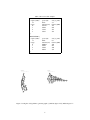
For example, Table 1 presents a table generated for by pe_write. Since table_cnt was set to two, there are two
tables that were generated. The first line contains the table label and the index of the first table. The next line is a
comment, because it starts with a “#” character. The line following it has 3 values. These values were set by the
table_attrib command. The following line contains another comment. The next four lines are set by the type_attrib.
Note, the first item in each line is the type number. Thus, these tables had two parameters listed for table_attrib and
two listed for type_attrib.
3.2
Original algorithm
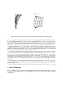
The original algorithm iteratively adds nodes to construct a graph using limits on the maximum in and out degrees of
each node. The file, origin1.eps, contains a task graph generated using the old algorithm with “in” and “out” degree
maximum value equal to two. By setting the “in” degree to one and the “out” degree to a higher value, a tree can be
generated such as the one in tree1.eps. These two files, origin1.eps and tree1.eps, are displayed in Figures 1(a) and
(b), respectively.
3.3
New algorithm
The new method is capable of generating several types of random graphs including series-parallel chains. sp_rand1.eps
is an example of a random graph that is generated using the new method. The file, sp_simple.eps, shows a simple example of a series-parallel task graph.
The series-parallel algorithm generates a root node that is connected to a set of chains of nodes. A chain of nodes is
one or more nodes that are linked together in series to form a chain. The algorithm gets its name, series-parallel, since
2 Those interested in reading more about this topic are referred to “Scheduling periodically occurring tasks on multiple processors” by E. L.
Lawler and C. U. Martel, in Information Processing Letters, vol. 7, pp. 9-12, Feb. 1981.
3
Table 1: Processor table example
PROCESSOR 0 {
# price (USD)
power (W)
area (sq. mm)
14
0.533
7.5
# type
run time (ms) memory (KB)
0
291428
348
1
36265
256
2
19323
312
3
43251
724
}
PROCESSOR 1 {
# price (USD)
11
# type
0
1
2
3
}
power (W)
0.648
run time (ms)
260032
36463
38269
26035
area (sq. mm)
6.9
memory (KB)
380
212
340
792
TASK_GRAPH 0
Period= 600
In/Out Degree Limits= 1 / 3
TASK_GRAPH 0
Period= 1000
In/Out Degree Limits= 2 / 2
0
0
1
4
1
2
2
5
3
3
4
6
7
11
d=300
8
9
10
18
19
5
12
6
8
10
11
13
14
d=500
9
7
13
15
d=500
17
24
27
d=600
d=600
d=600
16
22
d=500
20
21
d=400
d=400
23
25
26
28
29
d=500
d=500
d=500
d=500
d=500
12
16
17
d=800
14
15
d=900
d=900
18
19
d=1000
Figure 1: Using the old algorithm to generate graphs. (a) In/Out degree 2 2 (b) In/Out degree 1 2
4
TASK_GRAPH 0
Period= 1300
In/Out Degree Limits= 5 / 5
0
3
4
9
10
19
d=200
d=200
7
23
TASK_GRAPH 0
Period= 700
In/Out Degree Limits= 5 / 5
24
d=100
0
16
1
2
8
22
7
12
17
22
26
3
14
8
13
18
23
20
6
13
11
15
2
5
d=900
25
d=900
4
9
14
19
24
5
10
15
20
25
18
6
17
11
16
21
26
21
1
12
d=700
d=1300
Figure 2: Using the new algorithm to generate graphs. (a) Random graph (b) Series-parallel graph
the root node is attached to an arbitrary number of these chains of nodes. The number of chains and length of each chain
are set by the TGFF commands series_wid and series_len. Another parameter, series_must_rejoin, will generate an
extra (sink) node that will connect to the end of each chain. If that parameter is set to zero, series_subgraph_fork_out
allows the user to define the probability that these chains will not rejoin at the end. A root node connected to a set of
chains of nodes along with the corresponding sink node (if it is generated) is called an series-parallel unit (SPU).
The algorithm defined above is good for creating a few chains of nodes, but generates simple graphs. To make the
algorithm more applicable, it is performed recursively. The series-parallel algorithm first generates one SPU. If the
graph has less than the required number of nodes, one node inside the SPU is designated the root of a new SPU. This
process is repeated until the graph has the requested number of nodes.
To increase the generality of the task graphs generated using this method, parameters were added to generate
arcs between chains of nodes within a SPU and across SPUs. These commands are series_local_xover and series_global_xover. Used alone, these commands allow the user to generate a random graph that does not have seriesparallel structure. By setting the length and width of each SPU to 0 and using series_global_xover, a random graph
will be generated with only the number of edges specified by series_global_xover. An example based on this method,
sp_rand.tgff , can be found in the examples file. (Note that this is different from the sp_rand1.tgffopt found in this
directory).
By combining the random graph generation method with the series-parallel method, a wide variety of graphs can
be generated. The two files created using the new algorithm, sp_rand1.eps and sp_simple.eps, are displayed in Figures
2(a) and (b), respectively.
Note: The original algorithm is currently the default. To use the new algorithm, use the command gen_series_parallel.
4
How TGFF works
In general, TGFF accepts input parameters from a tgffopt file. A list of features TGFF currently supports are listed
below. It is recommended that new users examine the examples in Section 5 to get a basic understanding of how TGFF
commands work.
5
4.1
Usage
To invoke TGFF, use the following comand:
• tgff [filename]
4.1.1
Key
1. A ‘\’ can be used to enter multi-line commands.
2. A ‘#’ at the start of a line comments out the line.
3. Average and Multipliers: These multiplier indicate a value that is used to scale a random number [-1, 1) and
added to the average to obtain pseudo-random values. For example, an average of 4 with a multiplier of 2 ranges
from [2, 6).
4. Tasks and nodes are used interchangeably
5. Transmits and arcs are used interchageably
4.1.2
Datatypes
The following is a list of data types used for TGFF’s parameters:
• <string>: a string of characters
• <int>: an integer number
• <flt>: a floating point number
• <bool>: a boolean value which can be “true” or “false”
• <list(T)>: a comma separated series of zero or more values of type T
– Note: the parentheses are meta-characters — Don’t enter them!
4.2
Basic commands
• seed <int>: Sets the seed for the pseudo-random number generator.
– This allows users to command TGFF to create a family of closely related outputs by changing the random
number seed and leaving the other parameters constant.
4.2.1
Task graph generation
• tg_cnt <int>: Sets the number of task graphs to generate.
• tg_label <string>: Sets the (case dependent) label used for task graphs.
• tg_offset <string> <int>: Sets the start index for named task graph (default 0).
• task_cnt <int> <int>: Sets the minimum number of tasks per task graph (average, multiplier).
• trans_type_cnt <int>: Sets the number of possible transmit types.
• period_mul <list(<int>)>: Sets the multipliers for periods in multirate systems.
– Allows the user to specify the periods relative to each other.
– The multipliers are randomly selected from this list.
• prob_periodic <flt>: Sets the probability that a graph is periodic (default 1.0).
6
– Allows simultaneous generation of aperiodic and periodic task graphs.
• prob_multi_start_nodes <flt>: Sets the probability that a graph has more than one start node (default 0.0).
• start_node <int> <int>: Sets the number of start nodes for graphs which have multiple start nodes (average,
multiplier).
– If prob_multi_start_nodes is zero, this option is ignored.
4.2.2
Series-parallel commands (new algorithm)
• gen_series_parallel <bool>: If set, generate graphs with a series-parallel structure (default false).
– This command should be used to use the new graph generation algorithm.
• series_must_rejoin <bool>: If set, force subgraphs formed in series chains to rejoin into the main graph
– This overrides series_subgraph_fork_out flag.
• series_subgraph_fork_out <flt>: Sets the probability subgraphs will not rejoin.
• series_len <int>: Sets the length of series chains (average, multiplier).
• series_wid <int>: Sets the width of series chains (average, multiplier).
– This is the number of parallel chains generated for each node that is the head of a set of chains.
• series_local_xover <int>: Sets the number of extra local arcs added.
• series_global_xover <int>: Sets the number of extra global arcs added.
4.2.3
Old algorithm parameters
• task_degree <int> <int>: Sets the maximum number of transmits (degree) per task (in, out).
• task_type_cnt <int>: Sets the number of possible task types.
4.3
Table generation commands
These commands are used to generate the tables:
• entries_per_type <flt> <flt>: Sets the number of attribute entries per task type for tables (average, multiplier).
• table_label <string>: Sets the label used for the current table.
• table_offset <string> <int>: Sets the index for named table.
• table_cnt <int>: Sets the number of tables (of current table type) generated.
• type_table_ratio <flt>: Sets the ratio of statistical contributions of type to table attributes (default 0.5).
These three commands are similar in format:
• task_attrib <list(<string> <flt> <flt> <flt>)>:
–
–
–
–
name: Sets the name of the attribute to the value in string.
average: Sets an average value for the attribute.
multiplier: Sets the multiplier.
round to: Sets the probability for rounding to occur [0, 1) (Default 0.0, 0.0 means no rounding).
• table_attrib <list(<string> <flt> <flt> <flt> <flt>)>: name, average, multiplier, jitter (default 0.5) round to (default 0.0, 0.0 means no rounding)
• type_attrib <list(<string> <flt> <flt> <flt> <flt>)>: name, average, multiplier, jitter (default 0.5), round to (default 0.0, 0.0 means no rounding)
7
4.4
Output commands
These commands are used to output the task graphs and corresponding tables. TGFF generate output based on
current settings each time it encounters a write command. This leads to some interesting properties. Two sequential
write commands will cause output (to the corresponding output file) to be duplicated. A write command followed by
a modification, such as a new tg count, will cause the latter option to be ignored.
4.4.1
*.tgff file
• tg_write: Write the task graphs [to .tgff file].
• pe_write: Write PE information [to .tgff file].
• trans_write: Write transmission event information [to .tgff file].
• misc_write: Write independant processor information [to .tgff file].
– misc_type_cnt: Set the number of types for misc_write.
• note_write <list(<string>)>: Write the string(s) [to .tgff file].
4.4.2
*.eps file
• eps_write: Create a PostScript plot of the task graphs [to .eps file].
4.4.3
*.vcg file
• vcg_write: Creates an input file for the graph visulization tool VCG [to .vcg file].
– vcg_hide_edge_labels: Suppresses display of edge labels [for .vcg file].
4.5
Advanced commands
• period_laxity <flt>: Sets the laxity of periods relative to deadlines (default 1).
– Indicates whether task graphs deadlines are greater than, less than, or equal to the periods.
• period_g_deadline <bool>: If true, then periods values are forced to be greater than deadlines (default true).
• prob_hard_deadline <flt>: Sets the probability that a deadline will be hard (vs. soft).
• soft_deadline_mul <flt>: Sets the multiplier applied to soft deadlines (default 1).
– Used to increase create soft deadlines that are arbitrarily tighter than the hard deadlines.
• task_trans_time <flt>: Sets the average time per task including communication
– This value is used in setting deadlines.
• deadline_jitter <flt>: Sets the proportional jitter for deadline.
• task_unique <bool>: If true, tasks types are forced to be unique (false by default).
8
4.6
Untested legacy command
pack_schedule <int> <int> <flt> <flt> <flt> <flt> ... <int> <int> <int> <int> [<flt>] [to .tgff file & .eps file] [... on one
line]
• This is a ‘self-contained’ command, it generates PEs, COMs, TG, etc. Other writes except note_write should
not be used. Only non-periodic instances are generated, ‘task_degree’ and ‘seed’ are only cmds that affect its
operation.
• The args in-order are: num_task_graphs avg_task_graphs_per_pe avg_task_time mul_task_time task_slack
task_round num_pe_types num_pe_soln num_com_types num_com_soln and optionally arc_fill_factor.
• Note: VCG output is not available for this command.
5
Examples
The examples directory contains sample files that use TGFF to generate a variety of graphs and tables. The best way
to learn TGFF is to experiment by adding and removing options from these examples. The examples described below
can be found in the examples directory.
5.1
Basic example: simple.tgffopt
The first line in this file, tg_cnt 3, tells TGFF to generate 3 task graphs based on the parameters that follow. task_cnt 20
5, indicates that task graphs should have 20 tasks. The first number is the average value and the second is the +/- range
by which it can vary. (Note that the graphs generated by this file actually vary by more than this amount. This is caused
by the period_mul command, which is discussed below.) Since this file does not contain the gen_series_parallel
command, the old graph generation algorithm will be used. This algorithm uses the task_degree to indicate the
maximum number of incoming and outgoing arcs a task can have. In this case, tasks can have up to 3 incoming and 2
outgoing arcs.
The next two commands are slightly more complex. period_laxity represents how much slack there is in the
relationship between deadlines and periods. When set to it’s default value (1.0), the period of the task graph is equal
to the largest deadline. period_mul is used to influence the periodic relationship between the task graphs. The setting
in this file (1, 0.5, and 2), indicate that there is a 1:0.5:2 ratio between their periods. TGFF selects a value from the list
for each task graph generated and scales the period (and largest deadline) based on that value.
The next three lines are used to tell TGFF to generate output. This interface can be somewhat confusing at first, but
makes TGFF more general. For example, if a user wants to generate two sets of pe tables. Using explicit commands
for printing allows users to configure parameters once, print those tables, and then reconfigure the parameters and
print a second set of tables. One reason for doing this is that a user might want to generate pe tables with statistics for
processors and then another for FPGAs.
The next four lines configure table printing for the transmission (edges) table. The first line, table_label COMMUN, labels the table as COMMUN. The next line, table_cnt 3, indicates that three tables should be made based on
these parameters. table_attrib price 80 20, indicate that price is the only variable for the table. It’s average value
should be 80 +/- 20. type_attrib exec_time 50 20, indicates that each edge should have a value corresponding to the
transmission execution time. This value should be 50 +/- 20. Finally, trans_write indicates that the table should be
generated based on these parameters and then printed to file.
5.2
Other examples
As mentioned previously, the best method to learn TGFF is to experiment by adding, removing and modifying options.
kbasic_task.tgffopt and kbasic_tables.tgffopt are annotated example files that depict the basics of generating tasks and
tables, respectively. kseries_parallel.tgffopt and kseries_parallel_xover.tgffopt are basic examples of series_parallel
task graph generation. The latter of the two demonstrates how to use cross over edges. sp_rand.tgffopt shows how
to generate unstructured graphs using the new algorithm. Finally, kextended.tgffopt presents more advanced features.
These are the example source files that have been highly documented. There are other source files, but these are not
documented as well.
9