Download User's Guide for SIRENA II - Denis Alder

User's Guide for SIRENA II
A simulation model for the management of natural tropical forests
This document and the SIRENA model have been written by Denis Alder for CODEFORSA (Comisión
para Desarollo Forestal de San Carlos) under a consultancy supported by the UK Overseas Development
Administration.
Revised: 12-Jun-1997
Contents
Introduction ......................................................................................................... 1
Installation........................................................................................................... 1
Initial installation ...........................................................................................................................1
Setting up the user directory ........................................................................................................2
Updating SIRENA 2 .....................................................................................................................2
Obtaining updates on the Internet................................................................................................3
Starting Sirena 2 ................................................................................................. 3
The login screen...........................................................................................................................3
The localization dialog..................................................................................................................4
The menu system.........................................................................................................................4
Defining the forest basis for a simulation ........................................................ 5
The 'Base forestal' menu..............................................................................................................5
The processing of species codes.................................................................................................7
Creating inventory basis files .......................................................................................................8
Defining new inventory or sampling types ...................................................................................9
Species groups for forest management ......................................................... 10
General considerations ..............................................................................................................10
Managing species groups in SIRENA........................................................................................10
Specification of harvesting operations........................................................... 12
The ‘Aprovechamiento’dialog.....................................................................................................12
Scheduling and controls on the general intensity of harvesting ................................................13
Specifications for the selection of trees .....................................................................................14
Special options ...........................................................................................................................15
Specification of silvicultural treatments ......................................................... 16
The dialog screen.......................................................................................................................16
Timing of treatments ..................................................................................................................16
Special options ...........................................................................................................................17
Specifications for trees to be treated .........................................................................................17
The scenario manager...................................................................................... 18
Concepts and definitions............................................................................................................18
Using the scenario manager ......................................................................................................18
Setting general program options..................................................................... 20
The general options dialog.........................................................................................................20
Sensitivity analysis .....................................................................................................................22
Volume options...........................................................................................................................23
Output graphs ................................................................................................... 24
The species abundance graph...................................................................................................24
Size class distribution.................................................................................................................25
Volume by species groups over time .........................................................................................25
Harvested volumes ....................................................................................................................26
ii
Basal area dynamics..................................................................................................................27
Comparison of scenarios ...........................................................................................................28
Output tables.....................................................................................................30
Table of species by diameter classes ........................................................................................30
The yield table ............................................................................................................................31
Executive menu functions ............................................................................... 32
Running, pausing and cancelling simulations............................................................................32
Exporting and printing outputs ...................................................................................................32
Exiting from Sirena 2 ..................................................................................................................32
Technical basis of the model ........................................................................... 33
Introduction.................................................................................................................................33
The data base ............................................................................................................................33
The formation of species groups................................................................................................34
Growth and mortality rates by species groups...........................................................................36
The basal area increment model ...............................................................................................37
Basal area mortality ...................................................................................................................37
Recruitment basal area ..............................................................................................................38
Crown classification of trees ......................................................................................................39
Logging damage ........................................................................................................................40
Supplying coefficients to the model ...........................................................................................40
Conclusion: The application of SIRENA ........................................................ 42
Appendix: Troubleshooting ............................................................................ 43
iii
List of figures
Figure 1 The login screen ..............................................................................................................................3
Figure 2 The file selection dialog box used to locate a directory ..................................................................4
Figure 3 The SIRENA 2 menu system ............................................................................................................5
Figure 4 Dialog to select a forest basis file ...................................................................................................6
Figure 5 Screen for managing species groups .............................................................................................11
Figure 6 Screen to define harvesting options...............................................................................................12
Figure 7 Dialog for silvicultural treatment options .....................................................................................16
Figure 8 The scenario manager dialog........................................................................................................18
Figure 9 The dialog screen for setting general options ...............................................................................20
Figure 10 Settings for sensitivity analysis....................................................................................................21
Figure 11 Options for volume definitions ....................................................................................................23
Figure 12 The species abundance graph .....................................................................................................24
Figure 13 Graph of species groups by size classes......................................................................................25
Figure 14 Graph of standing volumes over time, by species groups ...........................................................26
Figure 15 Graph of harvested volumes ........................................................................................................27
Figure 16 Graph of basal area dynamics ....................................................................................................28
Figure 17 Example of the comparisons graph for three scenarios ..............................................................29
Figure 18 Screen showing the table of diameter classes..............................................................................30
Figure 19 Species groups formed around key species .................................................................................34
Figure 20 List of key species for Sirena 2 model groups .............................................................................35
Figure 21 Diameter increment and mortality coefficients by species groups ..............................................36
Figure 22 The basal area increment model .................................................................................................37
Figure 23 The basal area mortality model...................................................................................................38
Figure 24 The basal area recruitment model...............................................................................................39
Figure 25 Model for crown class classification ...........................................................................................40
Figure 26 Listing of the MODELS.SN2 coefficients file ..............................................................................41
iv
Introduction
SIRENA 2 is a simulation model designed to assist the management of natural tropical
forests. It is based on a preceding model, SIRENA 1, which was developed during 1996
for CODEFORSA under the UK/ODA Integrated Forest Management Project. The
scientific concepts around which the model are based are discussed in Alder (1995).
This document is a user's guide to the model, written for the forest engineers of
CODEFORSA, and for other potential users of the model.
SIRENA 2 is based on the analysis of tree growth patterns from data supplied by
CODEFORSA and from plots established and maintained by Portico SA. The data is
applicable in the northern zone of Costa Rica, covering drier forests principally in
CODEFORSA's managment area, and wetter forests under management by Portico. The
wetter forests are characterised by a high frequency of Carapa guianensis, whilst the
drier ones have Vochysia ferruginea as an indicator species. These two species do not
co-occur with any frequency. Pentaclethra macroloba is very common in both types of
forest.
Data from secondary forests was also supplied by COSAFORMA for use with the model,
but due to limited time, this has not been analysed substantially, and the model will
probably not reflect accurately regrowth from abandoned farmlands with its present
parameters.
Installation
Initial installation
Initial installation is made by a Microsoft-supplied installation Wizard from a set of three
disks. Separate installation kits are available for Windows 3.1 or Windows 95. In each
case Disk 1 of the set is placed in the A: drive, and the A:SETUP program run from
within Windows.
The SETUP program is automatic except with respect to the target directory. This
defaults to C:\SIRENA2, but another directory name can be typed instead if preferred. If
the installation is to a network, a directory on a shared drive or network server should be
specified.
The installation program copies any required DLL or other system files to the Windows
system directories, and creates the program Icon. During this process, error messages
may arise. The Ignore option should be chosen, and the installation will proceed to
completion. These error messages do not appear to affect the operation of the program.
The directory into which SIRENA 2 is installed is called in this guide the Sirena base
directory.
1
Setting up the user directory
SIRENA 2 can work with a variety of possible directory arrangements. The simplest is
to have all working files within the same directory as the SIRENA program itself. In this
case, no command line parameter is needed, and when the login screen appears, it should
be left blank, simply clicking OK or typing the {ENTER} key.
A second arrangement is to have several possible users, each with their own working
files including species list with customized groupings, scenarios, and outputs. These
users can each be assigned a sub-directory to the SIRENA directory. When logging in,
the user types his sub-directory name in the login screen.
A third possibility is to have the user directories located on another disk or drive. The
command line of SIRENA can have a parameter D=d:\path added which gives the deafult
base address. The user then only types the sub-directory at login. For example, in the
network installation at CODEFORSA, the following arrangment exists:
SIRENA base directory .........D:\APLIC\GENER\SIRENA2
User base directory ................X:\USUARIOS
Command line........................D= X:\USUARIOS\
User directories ......................X:\USUARIOS\DENIS
X:\USUARIOS\MAURICIO
X:\USUARIOS\RODOLFO\SIRENA
etc.
Login name ............................DENIS
MAURICIO
RODOLFO\SIRENA
etc.
The command line is set by editing the properties of the program icon from the Program
Manager in Windows 3.1. In Windows 95, the shortcut to the program is selected, and
the property keyword clicked from the menu or right mouse button.
When creating a SIRENA user directory, the file DEFAULTS.SN2 must be copied in to
the directory from the SIRENA base directory. This file contains details of the user’s
current preferences for the program.
Updating SIRENA 2
Updated versions can be installed by copying all the files on the update disk into the
Sirena base directory. This will usually include:
SIRENA2.EXE
IDIOMA.SN2
IDIOMB.SN2
MODELS.SN2
2
Obtaining updates on the Internet
Updates and original installation files can be obtained by E-mailing the author at:
[email protected]
Problems encountered during installation and operation can also be advised to this
address.
Starting Sirena 2
The login screen
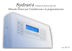
When the program is started by clicking on its Icon, a screen should appear as shown
below.
Figure 1 The login screen
The shows the characteristic background screen of Sirena 2, with a picture of forest
canopy. The window controls and text fonts for the main menu differ between Windows
95 and Windows 3.1. The login box offers the following options:
3
Nombre de usuário .......The user should enter a name corresponding to their user directory.
The base for the user directory is shown at the bottom left of the
dialog screen.
OK................................. Clicking this will start the program.
Cancelar ......................The program will close immediately.
The localization dialog
If the user's base directory has not been correctly specified with the D= parameter on the
command line (see page 2), then the login screen shown in Figure 1 will not appear
immediately. Instead a box will appear as shown below for selection of a directory. The
user can navigate this until the correct user directory is found, and then double click on it
and close the dialog. In some simple cases the program may then operate correctly. It is
more likely that the login screen will appear correctly, but some other file access
commands will fail at a later time with a system message such as 'Error 53 File not found'.
If installation has been done correctly, the localization dialog should not appear before
the login screen.
Figure 2 The file selection dialog box used to locate a directory
The menu system
Once the login screen has been negotiated, the program's system of menus will be
acessible. These appear as shown in Figure 3. The functional groups of menu choices
under the main headings are as follows:
Escenarios .............This group defines and reads in the forest data to be used as a basis for
simulation; establishes options for harvesting and silviculture; allows
the definition of species groups; and sets general options for program
4
control. These details can be saved as either program defaults (for the
general options) or as user-defined species lists (for grouping
methods), or as scenarios (for combinations of harvesting and
silviculture).
Gráficos .................This displays one of a number of possible charts or tables showing the
state of the forest, as the simulation progresses. These include graphs
of species abundance, size class distributions, volumes by species
groups, basal area by functional components, and a graph comparing
successive simulations.
Ejecución ...............This controls the exection of a simulation, starting, pausing, or
cancelling it. It also allows the current graphic to be copied to the
Windows clipboard for pasting into, for example, a Word document;
and allows a graphic to be printed in high quality mode directly to a
printer.
Figure 3 The SIRENA 2 menu system
Escenario
Ejecución
Gráficos
Base forestal
Abundancia de especies
Ejecutar
-
Distribución por clase de tamaño
Pausa
Grupos de especies
-
Anular
Aprovechamiento
Volumen por grupos
-
Tratamientos silviculturales
Volumen aprovechados
Copiar
-
Dinámicas de area basal
Imprimir
Manejo de escenarios
Comparaciones de escenarios
-
-
-
Salir
Parámetros de modelo
Cuadro de clases diámetricas
Cuadro de aprovechamiento
Selections from the menu are made in the conventional way with Windows, by pointing
and clicking with the mouse, or by using the underlined 'hot keys' from the keyboard.
Not all menus are initially accessible. Generally as a minimum, a file of forest data must
be read under the Base forestal menu before graphics can be displayed or a simulation run.
Defining the forest basis for a simulation
The 'Base forestal' menu
The necessary first step in running SIRENA is to read in forest data that will define a
forest to be simulated. The source of this data may be any kind of forest inventory or
permanent sample plot. The data is organized into text files with an extension .FBS
using a format that is discussed in more detail on page 8.
5
Sources of data may be of several types. For example, CODEFORSA uses Inventario
preliminar or Muestreo diagnostico data at present. The size, subsampling, and
associated species list for each type of plot may vary, and are defined in a control file
called INVTYP.SN2, which resides in the Sirena base directory. This is a simple text file
which can also be edited to add new sample types, as dicussed further below.
When the Base forestal menu bar is selected, a screen is displayed as shown below.
Figure 4 Dialog to select a forest basis file
The first field shows the current directory for forest files. This can be changed by
clicking the Cambiar button. A directory selection box appears similar to that in Figure 2,
but with the heading Buscar archivos de inventario. An alternative directory can be
selected, after which the use is returned to the Base forestal dialog.
The second field shows the current file type. Clicking the down-arrow at the right will
expose a list of available file types. Clicking on a member of this list will update the list
of displayed files in the third field.
The third field displays available files of the selected sampling type. Clicking one and
pressing Acceptar will load that file.
The loading process takes some moments. A count of plot numbers will appear in the
status display at the bottom of the screen. This can be used to verify that the file is
properly structured. In particular, blank lines in the data may be interpreted as 'false'
plots, and will reduce the overall estimates of stocking as a result of an overestimated
area figure for the sample.
6
After loading, the dialog screen will disappear. The name of the selected sample will
appear at the bottom left of the status display. All other menu options will then be
accessible.
The processing of species codes
When an inventory file is read, SIRENA first reads the species list specified by the
corresponding inventory types. This gives the codes used in the inventory, and their
corresponding local and latin names, the user-assigned species group, and a growth
model number.
SIRENA searches for the species list in two locations. The first is the user directory.
This will contain any copies of the species list that have been saved by the user with their
own system of species grouping. If no list is found in the user directory, it will then read
the list in the Sirena base directory.
The species codes are processed as text items, and may therefore be numeric, hierarchic,
or mnemonic codes of any type. CODEFORSA uses simple numeric codes.
If a species code is found in the inventory data which does not exist in the species list,
then SIRENA appends it to the internal list of the program. For example if species
number 999 was found in the data, but not in the list, it would append an entry with the
following details.
• A code number of 999, as found.
• A local name of 'Spp <999>'.
• A scientific name of 'Spp <999>'.
• A species group of 'X'.
• A growth model from the predefined default (from the MODELS.SN2 file).
This internal list is not automatically saved to file. It can be saved from the Grupos de
especies dialog, as discussed on page 10.
The procedure suggested for dealing with missing species codes and updating the species
list is as follows:
• Read several sets of inventory data. After each set, the species list should be saved via
the Grupos de especies menu. This will build a list of the common missing codes.
• Edit the species list in the user directory to insert correct local and latin names. The
species list can be read in to Excel and sorted by latin names to facilitate the editing of
an appropriate species group code. If the missing code is in fact a duplicate for an
existing code, then the growth model can be altered to that for the pre-existing entry.
Otherwise the default value should be left (this will probably be #36, subject to
revisions of the MODELS.SN2 file).
• If working with Excel, save the list again as a CSV file to the user directory.
• Check that Sirena reads the list correctly by opening files and viewing the stand table
to see that the species are now correctly named.
7
• From Windows or DOS, copy the species list back from the user directory to overwrite
the master list in the Sirena base directory.
Clicking the check box labelled Mostrar códigos de especies faltantes in Figure 4 gives a
screen displaying missing codes after a file has been read, with a count of the number of
occurrences of each code. Its use is not necessary for the operation of the above
procedure, but it does provide a quicker check than examining the species list with a text
editor.
Creating inventory basis files
The inventory files used by SIRENA are text files which are given the extension .FBS.
Normally the data will be extracted from a database file. At CODEFORSA for example,
the data may be held in the PLANMAN file called INV.DBF, or a file maintained by the
new TREMA system.
The most direct route for creating and FBS file is to extract the data from its DBF format
into a text file using FoxPro, and then edit it using a word processor to add the four lines
of header information that SIRENA requires.
A limited knowledge of FoxPro is needed to achieve the first step. It is necessary to
know the file containing the originating data, its full directory path on the system, and the
field names for the plot number, diameter, species code, and form/defect code. Given
this information, the following Foxpro commands will extract the data:
SET DEFAULT TO userdir
USE invpath\invfile
INDEX ON plot TO ~TEMP FOR forest=id
COPY TO outfile.FBS DELIMITED FIELDS plot, species, diam, form
where:
userdir .........................The full path of the user's directory for SIRENA work.
invpath .........................This is the full path of the inventory data file. On a network, the
user must have access rights to this path.
invfile ...........................This is the name of the .DBF file containing the inventory or
sample plot data.
plot ..............................This is the field name containing the sample plot number.
forest ...........................This is the field name containing the forest name or number.
id .................................This is a number or character string denoting the forest, farm or
sample to be extracted. If forest is a text field, it must be enclosed
in quotes. If forest is numeric, it should not be. A FoxPro error
message results if forest and id are not of compatible types.
outfile ...........................The name of the output file, with an extension .FBS added.
species ........................The field containing the species codes.
diam ............................The field containing tree diameters.
form .............................The field containing form or defect codes.
8
This method creates a temporary file ~TEMP.IDX in the user's directory which indexes
the required records from the database. This can be deleted if its presence is
inconvenient.
After creation of outfile.FBS it can be edited with a text editor to add the following lines of
information:
1. A code for the inventory type. INV and DIAG are defined for CODEFORSA
inventario preliminar or muestreo diagnostico, for example. New codes and
inventory types can be created as described in the following section.
2. A zero or a forest type code. This information is not used by SIRENA 2.
3. The title of the dataset. This can be any text.
4. A zero or the effective forest area. This information is not used by SIRENA 2.
The file should be checked with the text editor to ensure that there are no blank lines
between plots. There should also be no spare blank lines at the end of the file. The data
should be separated by commas, not semi-colons or any other delimiter. Decimal points
must be marked with the dot character, not a comma. None of the data needs to be
enclosed in quotation marks. Any quotation marks found should be deleted using the
search and replace function of the editor.
The file must be saved as a text only file. Saving it as a standard word processor file,
rich-text file, or other format will cause SIRENA to fail when reading the file.
Defining new inventory or sampling types
New inventory types are created by editing the file INVTYP.SN2 with a text editor. Each
line represents one type of plot. There are six items on each line, as follows:
1. The code used for the inventory, eg. INV.
2. The name for the type sample, comprising any descriptive text, eg. Muestreo
diagnostico.
3. The sample plot size in ha, eg. 0.3.
4. The smallest diameter, in cm, measured on the whole plot, eg. 30.
5. The size of a plot used for subsampling within the main plot to a smaller diameter
limit, eg. 0.075.
6. The name of the species list file applicable to the data, excluding the .SPL extension,
eg. CODFORSA.
9
Species groups for forest management
General considerations
Within the SIRENA 2 model, each species is represented individually* . However,
natural tropical forests typically comprise 300-400 species of which 50-100 may be of
commercial interest. In order to make prescriptions for harvesting and silviculture easy,
and in order to present ouputs and results simply, species need to be grouped. Generally,
the groups should comprise species with similar commercial demand and similar
management and silvicultural characteristics.
Groups appear in the legends of graphs and in other contexts where very long names are
not very helpful. Generally, the names given to species groups should be short
mnemonic codes of not more than 8-10 characters. The name of one group should not be
a complete subset of the name of another group. For example A and A+. SIRENA will
confuse group names if one is a subset of another. Group names are also sorted in
outputs and lists in alphabetical order. This may be borne in mind when devising group
names.
The graphic outputs use a built in scheme of colouring patterns for up to 6 groups.
Thereafter, the system resorts to default colours supplied by the graphics system. These
may not be very ideal, and may not be the same for different groups between graphs. It is
therefore better if possible to limit the number of groups to not more than 6.
Both these restrictions apply to SIRENA 2.10, and will probably be relaxed on later
versions.
Managing species groups in SIRENA
The menu Grupos de especies gives access to a dialog screen for moving species between
species groups, and for creating and deleting groups. This screen is shown in Figure 5
below.
Species can be moved between groups by clicking on them with the mouse to select
them, in either the left or right box, and then clicking on either of the arrows in the centre
to move them to the alternate box.
The group displayed in either box is selected from the pull down lists at the top.
A new group is created by over-typing the group name in the right-hand box, and then
clicking the button marked Anexar grupo nuevo. If no species have been selected in the
left-hand box, an empty group will be created. If species were selected in the left-hand
box , they will appear directly in the new group.
*
This was not the case with SIRENA 1, which worked only with pre-defined groups, and gave no access to
individual species.
10
Figure 5 Screen for managing species groups
A group is deleted by placing it in the left-hand box, removing all species from it into
other groups, and then clicking the button Suprimir grupo.
The button Borrar selección releases any species marked as selected.
If the two groups in the boxes are the same, the message “Grupos de especies deben ser
diferentes” will appear. Any action will be blocked until one of the groups is changed.
It is not possible with this screen either to duplicate or delete species from the list. They
can only be moved from one group to another.
The checkbox labelled Mostrar nombres cientificos will switch the naming between
scientific or vernacular names. However, it should be noted that typically many species
will not have vernacular names. For these, the generic name is shown enclosed in
brackets. Generally, the scientific names are more useful in this presentation.
The checkbox Hacer permanente los cambios is important. It causes the species list in the
user’s directory to be overwritten with the new groupings when the Accepter button is
pressed. A warning message precedes this to allow the user to change their mind.
With this facility, each user may therefore create a unique set of groupings. If a
particular grouping system is determined as being the definitive one, then the relevant
11
species list file (eg. CODFORSA.SPL) can be copied back into the Sirena base directory
from Windows.
There are some deficiencies in this dialog screen that will probably be remedied in later
revisions of SIRENA:
• The blocking function when the two lists are for the same group is unduly oppressive. It should be
relaxed to apply only to operations that move species.
• It is not possible to directly rename a group. Presently a new group must be created, the species copied
to it, and the old group deleted. This is rather tedious, and it is therefore important to spend some time
thinking out the nomenclature of groups prior to creating them.
Specification of harvesting operations
The ‘Aprovechamiento’dialog
Selecting the menu bar Aprovechamiento brings up the dialog screen shown in Figure 6.
Figure 6 Screen to define harvesting options
This screen allows various options relating to harvesting to be specified. The options are
divided into three functional boxes:
Control de aprovechamiento
This includes options which control the decision of whether to harvest or not,
and general limits on the number of trees or the basal area to be removed.
12
Selección de árboles
This covers the felling limits and retention specifications by species groups,
and determines the order of priority when felling species groups.
Opciones especiales
This provides a fast way of selecting a ‘no harvesting’ option, standard
operation, an option to pause the simulation after the harvest has been
performed for a more leisurely analysis of the various output screens, and an
option to switch to a different management regime (scenario) after the next
specified harvest.
These groups will be considered in more detail in the next sections.
Scheduling and controls on the general intensity of harvesting
In Figure 6, the box labelled Control de aprovechamiento includes the functions which
control the timing of harvesting. Each one has a check box on the left, and a value on the
right. Note that if the checkbox is not marked, that particular aspect of scheduling will be
ignored, regardless of any value in the field at the right. The options control harvesting
as follows:
Año del primer aprovechamiento
This specifies the first year for harvesting. Felling may be delayed after this
year if the third option, for basal area control, is also active and the required
basal area has not been reached.
Ciclo de corta
This specifies the felling cycle in years. Fellings will not be done over an
interval less than this period. If this box is not checked, no felling is done
unless the basal area control option is active.
Área basal requirido antes del aprovechamiento
This controls felling by basal area if it is checked. The stand cannot be felled
unless the specified basal area has been reached. If a felling cycle has also
been specified, then they will act together as constraints on felling, indicating
both a minimum period between fellings, and a minimum basal area that must
be reached. If no felling cycle is specified, then felling will be done whenever
the stand reaches the specified basal area.
Límite de número de árboles a cortar
This places a general limit on the number of trees per hectare that may be
removed during felling. It can be given as a fraction if required, representing
whole trees over a wider area. For example 2.5/ha indicates 25 trees on 10 ha.
Límite de área basal a cortar
This is an alternative to limiting felling by tree numbers. It specifies the
maximum basal area to be removed, in m2/ha. If both tree numbers and basal
area constraints are given together, the program will apply whichever
13
constraint is most severe in a particular harvest. However, this is likely to be
confusing to interpret, and is not recommended.
Specifications for the selection of trees
The group of options shown under Selección de árboles in Figure 6 determine the
specifications for felling. At least one line in this table must be checked with Sí in the
¿Cortar? column for any harvesting to be done.
Specifications for felling trees include the species group to be affected by a given rule,
the minimum diameter for trees to be felled, and the number or percentage of trees to be
retained. For each group in the table that is to be felled, the ¿Cortar? box should be
clicked with the mouse to show sí.
The retention can be specified either as a percentage of the standing trees above the size
limit for that species group, or as the total number of trees per hectare to be left. This is
done by clicking on one of the buttons to the right of the table.
The species group can be changed by clicking the mouse on the group name to make it
active, and then pressing the spacebar to cycle through the list of available groups. Note
that if the species grouping is changed, the specifications in this table do not
automatically reflect those changes, and it will be necessary to adjust the group names
and other details as required.
The order of groups in the table determines the priority of felling when a general limit
has been applied. If for example there is a general limit of 2 m2/ha, then all possible trees
from the first line of the table will be felled until the limiting basal area is reached. If it
has not been reached by felling these, then the process continues with the second line,
and so on. To achieve a proportional felling through a range of groups when there is a
general limit, a high Remnante is needed to ensure all trees are not taken from the group.
The order of species in the table can be changed using the up and down arrow buttons at
the lower left. This exchanges cells in a row from the active cell to the left with the row
above or below. If the cell selected is in the Grupo column, the whole row is exchanged.
If it is in the Diam column, the groups will remain as ordered, but the specifications will
be exchanged.
The current line in the table can be deleted by pressing the Ctrl+Del key. A new line will
be inserted by pressing Ctrl+Ins. A single cell is deleted by pressing Del. The deleted
text is stored in a memory, and will reappear in the active cell when Ins is pressed. This
can be used to rapidly enter the same figure in several cells. It is entered in the first cell,
and Del pressed to place it in the memory. Pressing Ins on each of the required cells will
then insert the figure.
The last column, header ¿Cortar?, can be checked or cleared by clicking with the mouse,
or by pressing the spacebar.
14
Special options
There are four special options available as alternatives:
Sin aprovechamiento
When this is checked, no harvesting is done. This is a quick way of
establishing a baseline for management without having to reset all the
individual options.
Normal
The controls and specifications are applied throughout the simulation.
Mode de pausa
The simulation stops after each harvesting has been done. It can be restarted
when required by pressing Ejecutar under the Ejecución menu. This option
provides a means of examining the graphs and tables which do not have a
time base before they change as the simulation proceeds. While the program
is stopped, the details of harvesting, silviculture, etc. may be modified to take
effect as the program is re-started.
Cambiar a escenario ...
This mode requires that the scenario manager has been used beforehand (see
page 18). If this is the case, then the pull down list will contain a series of
codes, which are the file names for scenarios. Selecting a code will cause the
program to switch to that felling regime after the first harvest in the current
specification. This process allows several quite different harvesting schedules
to be linked. Note that when a chained scenario is loaded, only the
harvesting specifications are updated; any silvicultural treatment will remain
the same. Silvicultural details can be chained separately, and operate in a
similar fashion, in that they only alter treatment rules and do not affect the
harvesting rules.
15
Specification of silvicultural treatments
The dialog screen
The dialog screen for specifying silvicultural treatments is invoked by clicking the menu
bar Tratamientos silviculturales. It has the same general layout and functions as the
harvesting dialog, with analogous options to control the timing of treatment and the
affected species groups.
Figure 7 Dialog for silvicultural treatment options
Timing of treatments
Figure 7 shows the layout of the screen. There are three checkboxes and associated value
fields related to the timing of treatment. Checking the Tratamiento inicial box causes an
initial treatment to be done in the specified year, irrespective of whether the stand has
been harvested or not. If this box is left clear, as in the example, then treatment is done
only after harvesting.
Treatment after each harvesting is specified by the second checkbox. The period in years
to elapse after each harvest is given in the field to the right of the label Tratamiento
después aprovechamiento. If this is zero, treatment is done in the same year as harvesting.
Treatments may also be repeated within a felling cycle by checking the third box,
labelled Repetir tratamiento después .... A value here of 5, for example, would repeat
treatment to the same specifications every 5 years.
16
Special options
The general options controlling treatment indicated in the group of buttons at the top
right of the screen (Figure 7) are the same as for the harvesting screen. The first button
provides a quick method of switching off treatment without having to edit the screen in
detail. The second button is for normal operation. The third causes the program to pause
after each treatment. It can be restarted from the Ejecutar menu bar. The fourth button
causes a new set of treatment options to be loaded as soon as the first treatment specified
has been performed. A more detailed account of these choices is given on page 15.
Specifications for trees to be treated
The table shown within the box labelled Diámetros y especies on the Tratamiento screen
(see Figure 7) allows the selected trees to be specified. Trees are selected by species
group (Grupo field), and must fall within a range specied by minimum and maximum
diameter (Dmin, Dmax fields). Of the eligible trees, only a certain percentage will
normally be treated (%raleo field).
For commercial species, it is unlikely that thinning treatment would be applied except to
trees of bad form or seriously damaged trees from past logging. This case can be selected
by clicking the mouse on the S/D field. It is not possible to combine on the same line a
phytosanitary specification with a percentage thinning, but it is possible to enter the same
group on two different lines. In this case, for example, one could specify the thinning of
all defective trees, and then a percentage of the remainder on a second line.
If the Dmax field is left blank, then all trees above the specified Dmin will be eligible for
thinning. If both Dmin and Dmax are blank, then all trees will be eligible for thinning
irrespective of size.
As with the Aprovechamiento screen, data can be stored in a memory by pressing Del, and
then re-inserted to the same and other fields by pressing Ins (see page 14). Lines in the
table can be deleted by pressing Ctrl+Del, and blank lines inserted with Ctrl+Ins. Moving
the cursor to a cell under the Grupo field and pressing the spacebar or clicking the mouse
will scroll through the currently defined species groups.
The S/D option cannot be toggled on or off (Sí or blank) if there is a figure in the adjacent
%raleo field. Likewise, data cannot be entered in the %raleo field if the S/D field
constains Sí.
Because there is no prioritization between groups for treatment, there is no control in this
table to change the order of groups, unlike the similar table on the Aprovechamiento
screen.
17
The scenario manager
Concepts and definitions
A scenario, in the terminology of SIRENA 2, is a combination of harvesting and
silvicultural treatments. The scenario manager allows scenarios to be saved to file,
recalled, or deleted from disk.
Each scenario has a title and a code, which is also used as the file name. The file name
consists of the code plus an extension of .SC2.
The scenario manager allows a standard list of harvesting and treatment regimes to be
kept on disk without needing to re-enter the details each run. As has been noted, both
harvesting and treatment specifications can include the linking of one scenrio with
another, to allow variable specifications which each felling cycle, and to allow variable
silvicultural treatments within a cycle. This gives the program almost complete
flexibility in the way treatments are specified.
The scenario manager can also be called up at any time while a simulation is running, to
introduce an immediate change in the management regime. This can be useful for testing
variable treatments and schedules in an ad hoc fashion.
Using the scenario manager
The scenario manager is called from the menu bar manejo de escenarios. The dialog
screen shown in Figure 8 appears.
Figure 8 The scenario manager dialog
A scenario is created by defining harvesting and treatment specifications using the
aprovechamiento and tratamiento screens discussed on pages 12 and 16. Once this has
been done, the scenario manager is invoked from the menu. The title box will appear
initially blank. A descriptive title of the regime should be typed in, bearing in mind that
18
this title will appear as a heading on output graphs and tables from the model. The
scenario should also be given a code, in a format suitable to serve as a file name. This is
typed in the Archivo window, which only allows letters and numbers up to a limit of 8
characters to be typed.
The scenario is then saved by pressing the Guardar button. If there is an existing scenario
with the same file name it will be overwritten without warning; if not, then a new file is
created. Checking the box marked Auto guardar does not save the scenario immediately,
but will cause it to be re-saved automatically in exit from the Aprovechamiento or
Tratamiento screens. This is done without warning regarding the overwriting of the
existing values.
Existing scenarios can be loaded by clicking on them from the list. This immediately
loads them in to memory. If the harvesting and treatment regimes have been edited
without saving them as a scenario, a warning message appears “Escenario actuel no
guardado. ¿Sobre-escribir?” At this point, the load can be cancelled and the current
scenario saved first, if required.
It is possible to load only the treatment, or only the harvesting component of a scenario
by checking one of the option buttons at the right of the screen. The default for manually
loaded scenarios is to load both components. If only a partial loading is requested, then
the part not loaded remains at its current value. For example, if under the Cargar options,
Tratar is selected, and a scenario is loaded by clicking on it, then the current harvesting
specifications will remain unchanged, but the treatment specifications will be overwritten
with those from the selected scenario.
A scenario is deleted by selecting it and clicking the Suprimir button.
Once a scenario has been selected, the dialog can be closed with Salir or by using the
conventional Windows close control.
19
Figure 9 The dialog screen for setting general options
Setting general program options
The general options dialog
Clicking the mouse on the menu bar Parametros de modelo produces a screen similar to
that shown in Figure 9. This is a tabbed dialog with three levels, the first of which is
shown when the screen first appears. This tab gives access to the following options:
Language
Checking either of the approriate option buttons switches all texts and
menus between the Spanish and English versions. Note that titles created
by the user for scenarios or data files are not translated.
Species names These may be either the scientific names of species, or their local names
where given in the species list (the name of the genus is substituted in
brackets where no local name is present).
Time controls These cover several aspects of model operation. The Limite de tiempo is
the total simulated time the model will run for. Actualizar graficos
determines the frequency with which graphs are updated. Unir cohortos
merges cohorts internally at the intervals inidcated. A value of about 10
years will probably give optimal program speed. Ajustar copas determines
the frequency with which the crown classes of cohorts are recalculated.
This should not be more than 5 years, and on faster computers can be
20
reduced to give smoother lines on the graphs. The Ancho de cohortos is not
strictly a time control, but effects program speed and resolution. A value
of 2 cm is recommended on slower machines, and 1 cm on faster ones
with the 32-bit version of the program.
Diameter classes The diameter classes used in output tables and graphs can be set by
typing in lower bounds in the box labelled Límite mínimo por clase
diámetrica. These values must be separated by semi-colons, not commas.
There is no special limit on the number or size of classes, and these values
can be changed while the program is running. However, outputs will
become congested if too many classes are chosen; the program may fail if
there are less than 2 classes; and the lowest class should not be less than
10 cm, as lower classes are not created by the model with its current
growth model calibration.
Form codes
The form codes that occur in the inventory data representing trees that are
acceptable for harvesting should be shown in the box labelled Codigos de
forma ... Several values may be entered, but they must be numeric (not
text codes), and they must be separated in the list by semi-colons. Any
form codes other than those listed will be deemed to mark a tree as
defective, either due to damage or bad form.
Figure 10 Settings for sensitivity analysis
21
Colour output Graphs will be printed in colour, as they appear on the screen, if the box
labelled Imprimir en color is checked. This generally works better than
black and white printing with laser and HP Deskjet-compatible printers.
In the present version, the patterns selected by default for black and white
printing are little confusing. When graphs are copied to the clipboard, this
is always done in colour as a metafile image. This can be edited with
various picture editors, including that in Microsoft Word.
Saving options Checking the box labelled Guardar como formato will save the options into
the file DEFAULTS.SN2 in the user directory when the Acceptar button is
pressed . The existing file of this name will be renamed as DEFAULTS.01!,
02!, etc., each time the file is saved. These backup copies can be deleted
from time to time. They are intended as a safeguard, as inappropriate
values for some of these general options can make the program
unrunnable.
Sensitivity analysis
The second tab of the Opciones general screen, labelled Sensibilidad, reveals several
parameters which can be varied to test the sensitivity of the model, or to adjust its
calibration to different sites or situations (see Figure 10). Each value is a multiplier for
the basic model referred to. For example, replacing the value of 1 in the Crecimiento
diametrico with a value of 1.1 will increase all diameter increments by 10%, subject to
other constraints in the model.
These factors should not be set to values other than 1 for normal use. The only field that
may be applicable for general forest management is that for logging damage (Daño de
aprovechamiento), which may be adjusted to test the implications of more or less
damaging regimes. However, it should be appreciated that coefficients outside the range
0.7 to 1.3, implying a 30% reduction or increase in typical damage, are unlikely to be
realistic in any context.
Large values for these sensitivity factors may make the program unrunnable.
22
Figure 11 Options for volume definitions
Volume options
Selecting the third tab from the Opciones general screen, labelled Volumen, give access to
settings for calculating and displaying volumes. The general volume equation
coefficients are for a logarithmic equation with the form:
Volume = α.Diamβ
with volume in m3, and diameter in cm.
The Límite mínimo... field gives the smallest diameter tree that will be included for volume
calculations on the graph of standing volumes. The Especies para comparaciones should
be a list of species groups, separated by commas (not semi-colons in this case), to be
included in the volume calculation for the lines on the graph comparing successive
simulation runs. The group names are case sensitive. If a group is given here which is
either misspelt, or does not correspond to an existing group, no error is reported, but no
volume is calculated.
The Diam> field for the comparisons line shows the tree sizes to be included in
calculating the comparisons volumes.
23
Output graphs
The species abundance graph
The species abundance graph is displayed by clicking the line labelled Abundancia de
especies under the Gráficos menu. An example of this graph is shown in Figure 12 below.
The most abundant species is listed first, proceeding down the graph to the least
abundant. Scientific names are abbreviated to the first 5 characters of the genus and three
of the species, all capitalized. If the use of local names is requested, these are
abbreviated to approximately 12 characters where necessary by appending an ellipsis
(...). Options appear next to the graph which allow several aspects of its appearance to be
changed. The graph can show abundance in terms of numbers per hectare, or basal area
%. The trees included can be set to include only those above a specified minimum
diameter. The number of species to be shown can be set. In general, with more than 1520 species shown, the text for the left axis may become too small to be readable.
This graph is a very useful indicator for characterising the type of forest being simulated,
with its predominant species. If the model is run while the graph is displayed, it will be
seen to changed dynamically with each simulated year. The year is shown in brackets on
the title line.
Figure 12 The species abundance graph
Sin Aprovechamiento : Ferlo II (Año 0)
PENTA
MAC
CARAP
GUI
VOCHY
FER
DIALI
GUI
TERMI
AMA
ATTAL
BUT
GUARE
BUL
BROSI
LAC
Otras especies
0
10
20
Area basal %
24
30
40
Size class distribution
The graph showing size class distributions by species groups is invoked using the menu
bar Distribución por clase de tamaño. An example is shown in Figure 13 below. The size
classes used are set from the general options screen, as discussed on page 20. The left
axis can be set to show trees/ha, basal area/ha, or volume/ha. The graph is updated
dynamically as the simulation runs, and shows the current year as part of the title.
Figure 13 Graph of species groups by size classes
Ferlo II : Sin Aprovechamiento (Año 0)
5
Area
basal
(m2/ha)
4
Comercial
3
Exoticas
Gavilan
2
Nocomercia
1
Palmas
0
10-20 30-40 50-60 70-80 90+
20-30 40-50 60-70 80-90
Potencial
Diameter class (cm)
Volume by species groups over time
A graph of standing volume by species groups, as it develops over simulated time, can be
shown from the menu selection Volumen por grupos. An example of this graph is shown
for a regime with a felling cycle of 10 years, and extraction limited to 3 m2/ha in Figure
14. In this example, only Gavilan and the Comercial group are being felled. There is a
decline in the stock over time, but it appears to stabilise over about 50 years. It is
probable that a felling controlled to remove a lower basal area would be more suitable on
such a short felling cycle.
The volumes are calculated down to the limit specified under the Volumen tab of the
Opciones general screen (see Figure 11). In this case, volumes are shown for all trees
above 40 cm diameter. The lines are cumulative, so the volume for an individual species
should be worked out by taking the difference between its line and the preceding line
25
below. The time axis will always depend on the time limit for the simulation, whereas
the volume axis is set automatically.
Figure 14 Graph of standing volumes over time, by species groups
Aprovechar cade 10 años, 50cm+, 40% rem, 3 m2/ha lim. : Ferlo II
200
Comercial
150
Exoticas
Volumen
(m3/ha) diam
100
40cm +
Gavilan
Nocomercial
50
Palmas
0
0
10
20
30
40
50
Potencial
Año
Harvested volumes
The graph of harvested volumes is produced by selecting the menu bar Volumen
aprovechados. This shows a bar for each felling cycle, subdivided into quantities for each
species group, as illustrated in Figure 15. The values are cumulative, and show the
volumes actually extracted. The volume of an individual species will be the difference
between the top and bottom values for its section of the bar. The topmost section shows
volumes destroyed, for all species, among the remnant population, due to skid trails,
felling gaps, and severe damage to standing trees.
This example shows a typical pattern of yields in which the most valuable species tend to
be taken in the earlier cycles, and less valuable ones in later cycles. The graph also
shows a moderate decline in yields over time. These tendencies of a simple management
regime can be corrected by placing more stringent limits on the proportion of valuable
species removed, and by somewhat reducing the overall level of harvest.
It should be noted that the felling damage shown on this graph is calculated for all
species and for all size classes represented in the simulation. This will be down to 10 cm
diameter in the present version. It illustrates the point that any felling carries with it a
significant cost to the remaining growing stock, in terms of trees and volumes lost.
26
Figure 15 Graph of harvested volumes
Aprovechar cade 10 años, 50cm+, 40% rem, 3 m2/ha lim. : Ferlo II
40
Comercial
30
Exoticas
Volúmenes
aprovechados
20
(m3/ha)
Gavilan
Nocomercial
Palmas
10
Potencial
0
5
15
25
35
45
Volumen dañado
(todos especies)
Año
Basal area dynamics
The graph of basal area dynamics is invoked from the menu bar Dinámicas de area basal.
It illustrates the components of the stand that the model uses in its calculations to
estimate growth. An example of this graph, for the same management regime as the
preceding cases, is shown in Figure 16.
The standing basal area is subdivided into trees of the upper canopy, corresponding to
crown classes 4 and 5 according to Dawkins system, and the lower canopy, or crown
classes 1-3. Defective trees of either category are shown above these two layers. This
includes trees of bad form, or trees which have been significantly damaged by logging.
Each of these three layers has its own distinctive species-dependent growth and mortality
function within the model. Generally, most active diameter growth occurs in the upper
canopy trees. When running the model, it may appear that the lower canopy basal area is
increasing, whilst that of the upper canopy remains relatively constant. This results from
the fact that as the upper canopy trees grow, the smaller ones will be pushed into the
lower canopy by competition, and hence will become more static in their diameter
growth. In the process, the proportion of the stand basal area in the lower canopy will
tend to increase.
Above the standing basal areas are shown thin sections which indicate recruitment,
increment, and basal area losses through mortality. Harvesting and treatment are shown
as triangular peaks on the bottom axis of the graph, which are deducted from the standing
basal area.
27
It will be noticed that the line between upper canopy and lower canopy basal areas tends
to be somewhat jagged. This is a function partly of the harvesting process, in this
instance, as trees are removed or destroyed, but it is also a function of the frequency with
which crown classes are recalculated. The options screen (Figure 9) allows the frequency
for recalculating tree canopy positions to be adjusted. This is quite a slow process within
the model, and typically can be done on a 5-year cycle. However, if a smoother, more
natural looking graph is required, it can be set to an annual basis. This will however slow
the model down and does not much influence overall accuracy.
Figure 16 Graph of basal area dynamics
Aprovechar cade 10 años, 50cm+, 40% rem, 3 m2/ha lim. : Ferlo II
30
25
Aprovechamiento
Tratamiento
20
Dosel superior
Area basal (m2/ha)
15
Dosel inferior
Defectuosos
10
Ingresos
5
Crecimiento
0
0
10
20
30
40
50
Mortalidad
Año
Regardless of the adjustment frequency set, crown positions are always recalculated
following any disturbance of the stand due to logging or treatment. Some trees will then
be promoted to upper canopy status to compensate for losses, in effect simulating the
process of gap formation.
Comparison of scenarios
When successive simulations are run, the volumes for a defined component of the forest
in each trial are plotted on the comparison of scenarios graph. This is invoked from the
menu bar by clicking on Comparaciones de escenarios. The actual volumes included in
this graph are determined from the settings in the Opciones general : Volumen screen,
discussed on page 23. This determines the lower diameter limit for the volume shown,
and the list of species groups to be shown. It is important that the names of the species
groups correspond exactly with current groups, as otherwise nothing may appear and the
comparisons line will simply lie along the zero axis. These names are cases sensitive, so
that capital and small letters must correspond.
28
The example shows three regimes. The first is for the forest without harvesting. This
shows a rise in volumes over 50 cm to about 100 m3/ha after some 35 years, where it
stabilises. The second corresponds to the preceding examples, with 3 m2/ha being
removed on a 10-year cycle. The third is an attempt at a more sustainable method of
harvesting. The retention percentage is increased to 60%, and felling is scheduled when
the stand reaches 25 m2/ha, but removals are still 3 m2/ha. It shows a very similar
pattern to the second regime, with declining large tree volumes over time, as the stock is
effectively consumed non-renewably.
Figure 17 Example of the comparisons graph for three scenarios
Volumen de árboles 50+cm dap para especies Comercial,
150
(1) Sin Aprovechamiento
100
m3/ha
(2) Aprovechar cade 10 años,
50cm+, 40% rem, 3 m2/ha lim.
50
(3) Aprovechar a 25 m2/ha,
50cm+, 60% rem, 3 m2/ha lim.
0
0
10
20
30
40
50
Año
The title to the comparisons graph will show the volume limit and the species groups
selected in the Opciones general screen. The legend shows the individual scenario titles.
This requires that the scenario is saved via the Manejo de escenarios; otherwise, only run
numbers are shown, and the legend text is blank. This graph is not well suited for
monochrome reproduction, due to the similarity of the lines.
29
Output tables
Table of species by diameter classes
Clicking on the menu bar Cuadro de clases diámetricas brings up a screen like the example
shown in Figure 18. This displays initially a stand table for species groups. It has
several active functions. The statistic shown in the table may be N/ha, volume, or basal
area. Volumes, if selected, are calculated to the lower diameter limit set under the
Opciones general : Volumen screen.
Figure 18 Screen showing the table of diameter classes
The table shows data for trees of acceptable form only, defective trees only, or both,
depending on the value selected under Forma.
The boxes labelled Totales provide a calculator function that is useful for analysing
harvesting and treatment specifications. If a group of cells are selected with the mouse,
as shown in the example, then the totals for this group will be displayed in the box
labelled Selección. Clicking on the Selección field adds this total to any value already in
the Acumulado field, and clears the Selección field for a new value. The Acumulado field
itself can be cleared by double-clicking it. These functions are useful for totalling values
for particular species within a range of diameter classes.
30
The table initially shows summaries by species groups. Double clicking the mouse on a
line expands the table for that group to show the data species by species. Double clicking
again causes the table to revert to its original form, showing group summaries.
The stand table data can be saved to a text file that is readable by Excel. It is necessary
before doing this to assign a scenario name to the simulation, using the scenario manager.
The check box labelled Escribir cuadro a archivo will then become accessible. A default
file name consisting of the scenario code, followed by the year as an extension, will be
shown in the text box. This name can be edited manually. When the check box is
clicked, the file is written, and at the bottom of the screen, the full output path and file
name will be shown.
The file contains heading information giving the forest and scenario name, the statistic
used (N/ha, volume, or basal area), and the type of trees included (acceptable, defective,
or both), as well as the current year. It then lists each species with its code, name, and
group, and the stock by diameter classes.
This table can be imported into Excel very easily using default options. The file is
opened as if it were a spreadsheet. A ‘Wizard’ will then appear. Select immediately the
‘Finished’ button at the lower right to indicate acceptance of all default settings, and the
table will be imported correctly. The table can then be formatted, edited and sorted as
required, and saved as an Excel workbook under another name.
If the screen is displayed while the model is running a simulation, then the displayed
values will be updated automatically for growth, mortality, etc. The model can be
paused and the table saved to file as required. Each time it is saved, the file name
extension will automatically be adjusted to reflect the simulation year.
The yield table
All the figures that underlie the graphs of standing and harvested volumes can also be
saved to file as the model is run. This requires that a scenario name is selected
beforehand using the scenario manager. The menu bar Cuadro de aprovechamiento is then
chosen. A tick will appear beside the bar in the menu to show that this feature is active.
Outputs from the model will be saved into a file with the same name as the scenario code,
but with an extension .SY2.
This file can be imported into Excel in the same way as the diameter class table, as noted
above. The file is opened in Excel, and the text import Wizard will automatically format
the file using its default options. The file contains a heading giving the forest name, the
scenario title, and the headings for the various data columns. The rows in the file
correspond to years in the simulation. The data can be edited as required for
presentation.
31
Executive menu functions
Running, pausing and cancelling simulations
Under the menu heading Ejecución will be found three groups of functions which control
execution of the model, exportation of outputs, or the exit from the program
Ejecutar runs the model with currently defined parameters. If the model has not yet been
started, or has finished (with FIN displayed in the lower right box of the status bar), then
it will start from year zero. If the model has been paused, then it will continue from the
year at which it paused.
Pausa halts the model temporarily. It can be restarted by clicking on Ejecutar again. It
will continue from the year in which it was paused. While the model is paused,
harvesting and silvicultural options can be changed, the scenario manager accessed, and
any of the output screens examined. Outputs can be printed or copied to the clipboard as
required.
It is also possible to change species groups while the model is running or to import new
forest data. This is definitely not recommended however, and may cause the program to
fail. If it is desired to do this, then the Anular option should be used beforehand, or the
model allowed to finish its run (indicated by FIN on the status line).
Anular cancels an active simulation and returns the year to zero, reloading the base line
data for the forest.
Exporting and printing outputs
The menu bars Copiar and Imprimir act on a currently displayed graph, if there is one.
Copiar copies the graph to the Windows clipboard as a metafile. This can be imported
into Microsoft Word as a picture object, and may be edited within Word to a limited
extent. A number of graphics packages can also import this format and may allow more
facile editing. Using Word, it is simply necessary to click the Copiar bar, switch to Word,
and press CTRL+V at the point where the graph is to be pasted in to the document. Double
clicking on the graph will invoke the Word picture editor for minor embellishments.
The Imprimir function sends a high-quality image of the graph to the system default
printer.
These functions work only on graphs. They do not print or copy either the stand table, or
any of the input screens. The stand table can be output via Excel, as discussed on page
30 above.
Exiting from Sirena 2
Clicking the Salir menu bar causes the program to be terminated. This can also be
effected by closing the main program window, or with the ALT+F4 key.
32
Technical basis of the model
Introduction
It is not necessary to read this section in order to use SIRENA. It is intended to provide
background information on how the model works. A more technical discussion of cohort
modelling in general will be found in Alder (1995).
The data base
The basis for analysing the growth functions in the model were 9 1-ha and 27 ¼-ha plots
established by CODEFORSA since 1991, with an average remeasurement period of
about 4 years, and 17 1-ha plots established by Portico SA since 1989, measured over
about 7 years, in all cases with 2 or 3 intermediate measurements. The same data was
used in the SIRENA I model, but in this instance intermediate measurements have been
used, and the latest remeasurements for 1995 and 1996 added to the data set.
In addition to this, COSAFORMA provided measurements from 34 plots of 600 m2
established in secondary forest. These plots were included in the tree increment analysis,
but were not used in the basal area functions due to their small size. These plots were
measured annually over a 4-year period from 1992.
In all, a total of 64,678 tree records exist in the database, covering 624 species. There are
three distinctive types of forest:
• The CODEFORSA plots occur mainly in the central northern zone of Costa Rica, and
are characterised by somewhat lower basal areas (typically 20-25 m2/ha), the presence
of Vochysia ferruginea as an indicator, and the relative absence of Carapa guianensis.
The forests in which the plots are located are mostly smaller fragments of about 50100 ha.
• The Portico plots occur further to the east, in higher rainfall areas, in larger continuous
tracts of forest, and are characterised by a high frequency of Carapa guianensis and
the absence Vochysia ferruginea.
• In both types of forests, Pentaclethra macroloba is a very common component,
typically constituting 30-40% of the basal area in many cases. Its abundance is
generally lower in the Portico forests, however.
• The secondary forests of the COSAFORMA data set are young regrowth stands of
various pioneer species. A distinctive aspect is the frequency of Cordia alliodora, and
the relative absence of Pentaclethra, Vochysia, or Carapa. These plots are also
located in the central northern zone of Costa Rica.
The present version of the model is therefore limited in its applicability to these forests of
the northern zone of Costa Rica.
33
The formation of species groups
The formation of species groups is a necessary first step in analysing growth functions
for any tropical forest data. This is because there are a large number of species, many of
which are represented in the data by only a few individuals.
For the SIRENA 2 data, methods were tried based on statistical comparisons of
regressions between species. Initially, species that were rare were grouped by genera to
achieve at least 5 or 6 individuals. A logarithmic regression of basal area increment on
tree basal area was then fitted. Using as a discrimination factor a 95% probability that
two groups differed, some twenty groups were formed, containing very unequal numbers
of trees, and combining species with no apparently similar attributes. The method was
not felt to be very useful as it did not combine naturally species that ought to be similar,
such as fast growing, shorter lived species, or slower growing, longer lived types.
As with past modelling efforts with SIRENA 1, and the CAFOGROM models for Brazil,
a more pragmatic method was eventually used, in which mean increment of upper canopy
trees (classes 3-5) was graphed against the largest observed individual for each species.
This naturally groups short-lived, fast growing ephemerals, and larger, slower growing
forest trees. In order to make the grouping as consistent as possible with common-sense,
the groups were formed by identifying key species scattered over the ordination space.
Other species were then assigned to the groups seeded from these key species on the
basis of their distance.in ordination space. Thus each non-key species was attached to a
group formed by the nearest key species.
Figure 19 Species groups formed around key species
Mean increment (cm/yr)
3.00
22
2.50
CROTO SMI
22
22
24
OCHRO LAG
24
24
2.00
24
17
17
17
17
CROTO KIL
17
1.50
17
25
25
CECRO OBT
25
25
25
1.00
5
25
25
25
25
15
10
25 25
15
15
15
15
VOCHY
ALL
6
10
1515
TERMI AMA
10
10 10
15 GUI
30
TAPIR
30
15
15
3030
3030
5
30
303030
18 15
18
8
18
18
30
CORDI
POR18
30
30
30
30
13
30
18 18 PAN
30
PROTI
VIROL KOS
30
18
8
8
1818
8
18
28 28
30
13
18
28 28
13
28
MINQU
GUI
99
21
28
21
28 2121
21
QUALE PAR
13
2828 28INGA
28
13 13
THI
9
13 11
31
21
MOSQU JAM
21
11 11
28
31
31
21 21 21 21 21 13 131111
31283121
31
CORDI
ALL
PUN
31 31 MICON
21
11
21
7
11
16 16
31 31 31 26 26
11
26 26 2126
16
31 3131
26
26
26
16 16 11
26 16 16 16
7
26CASEA
7
32 323131 26 26 26
16
TABEB
7
ARB
12
14
3232
26 26 1616
16
26 26
16
32 2626
16
12
161616 SIMIR
16
16
7
26 LAT
32
32
141412
MAX
32
7
32
32 32
32
16
16 16
CHIMA
27
3232
27
12 12
3232 32 32
14
12
32 32
2727 272727
2727
16
7
19
16 16
LAETI12
PRO
32
GRIAS
CAU
HENRI
ODO
34 34
19
12
27
19
12
27
12
14
12 12
34 27 27 2727
19
1919 19
14
1414
34 34
FERDI
PAN
14
27
34
19
19
34
34
27
34
34
34
27
27
34
14
3434
34LONCH GUA
19
29 27 19 19 19
14
19
12
3434
3434
292929 2929
34 343434
29
14
19 19
34
29
23
2929
14
23
2929
23 COS
33 3333
23
3333332929
2323
29 ESCHW
20
23
2929
33 33
3333
29
33
33
23 23
29 23
CHION
COS
3333 33
33
GON
2323 DENDR
20BROSI RUB
33
3333
33333333 33
20
33
3333
3333
33
33
20 20
33 33
23
23 23
30
5
VOCHY FER
30
0.50
.00
0
20
40
60
80
PENTA MAC
4
7
ROS
DIPTE PAN CARAP GUI
PTERO OFF
1
4
4
7
100
120
Maximum diameter (cm/yr)
34
140
160
180
200
The results of this ordination are shown in Figure 19. The key species that ‘seed’each
group are shown by a circle, with their abbreviated species name. The small numbers
show the position of other species associated with each group. The table below lists the
groups, with their key species and other statistics.
Figure 20 List of key species for Sirena 2 model groups
Group
0
1
2
3
4
5
6
7
8
9
10
11
12
13
14
15
16
17
18
19
20
21
22
23
24
25
26
27
28
29
30
31
32
33
34
Key species
Palms
Pterocarpus officinalis
Carapa guianensis
Pentaclethra macroloba
Dipteryx panamensis
Vochysia ferruginea
Vochysia allenii
Tabebuia rosea
Virola koschnyi
Qualea paraensis
Terminalia amazonia
Cordia alliodora
Laetia procera
Minquartia guianensis
Grias cauliflora
Tapirira guianensis
Simira maxoni
Croton killipianus
Protium panamense
Ferdinandusa panamensis
Brosimum rubescens
Mosquitoxylon jamaicense
Croton smithianus
Dendropanax gonatopodus
Ochroma lagopus
Cecropia obtusifolia
Casearia arborea
Henriettea odorata
Inga thibaudiana
Eschweilera costaricensis
Cordia porcata
Miconia punctata
Chimarrhys latifolia
Chione costarricense
Lonchocarpus guatema
Trees
247
1147
1651
52
221
156
60
133
150
16
118
242
16
110
80
267
28
110
276
14
55
52
30
59
15
98
94
52
28
17
50
57
17
44
Dmax
195
133
121
118
108
86
89
80
76
70
68
69
58
51
49
46
41
41
44
43
35
30
31
27
28
30
26
23
22
17
18
19
16
15
Dinc
0.61
0.62
0.77
0.59
0.93
1.23
0.41
0.73
0.61
1.09
0.51
0.29
0.64
0.28
0.98
0.34
1.77
0.73
0.22
0.04
0.56
2.41
0.06
2.24
1.30
0.40
0.28
0.59
0.10
0.78
0.51
0.33
0.07
0.18
Nsp
18
3
1
1
4
4
2
10
5
4
6
10
15
11
14
13
26
7
14
18
7
17
6
16
5
15
24
27
17
25
31
22
33
65
44
The number of trees shown under the Trees heading refers only to the number of trees for
the key species, not for all the species in the group. Likewise, the statistics shown are for
the key species only, not group means. The last column shows the number of species in
each group. Statistics are not shown for palms, as these were grouped on the basis of
their botanical affinity, rather than via the ordination process.
The species group that each individual species belongs to is contained in a database file
called GROUPS. This has two fields, GENSPP and GRUP, which give the abbreviated
scientific name of the species, and its allocated group. This file can be used as a resource
to add group numbers to any species list that is being prepared for use by SIRENA.
35
Growth and mortality rates by species groups
Once species groups had been determined, it was possible to compile increment and
mortality data and fit regressions. In the event, it was found that tree size was not a
significant factor in tree increment regressions once canopy position and defect status had
been accounted for. Increment statistics were therefore compiled as a simple table of
mean increments for lower canopy trees (crown classes 1-3) , upper canopy trees (crown
classes 4-5), and defective trees (malformed, damaged, or trees which died over the
period). Mortality statistics were compiled on a similar basis. The ceofficients are
shown by species groups in the table below.
Figure 21 Diameter increment and mortality coefficients by species
groups
Species
group
0
1
2
3
4
5
6
7
8
9
10
11
12
13
14
15
16
17
18
19
20
21
22
23
24
25
26
27
28
29
30
31
32
33
34
Total
trees
7370
952
2754
4326
636
636
443
565
568
621
282
944
1225
453
784
479
1665
24
511
1792
100
520
149
693
118
78
910
1413
353
930
269
320
445
534
560
Dbh increment, cm/yr
U/S
Canopy Defective
0.083
0.061
0.027
0.323
0.706
0.518
0.230
0.629
0.293
0.656
0.866
0.467
0.297
0.430
0.463
0.560
1.029
0.467
0.525
1.375
0.344
0.194
0.346
0.156
0.404
0.754
0.117
0.344
0.645
0.354
0.876
1.161
0.342
0.384
0.511
0.571
0.200
0.341
0.115
0.401
0.652
0.375
0.226
0.276
0.138
0.543
1.033
0.616
0.272
0.392
0.155
0.476
1.457
3.425
0.368
0.924
0.672
0.178
0.198
0.133
0.233
0.124
0.051
0.318
0.657
0.167
1.164
2.683
1.507
0.199
0.102
0.088
0.953
2.387
1.755
1.099
1.227
0.000
0.379
0.391
0.253
0.256
0.257
0.213
0.466
0.757
0.388
0.176
0.142
0.021
0.466
0.904
0.384
0.366
0.406
0.301
0.335
0.280
0.178
0.101
0.104
0.118
0.220
0.168
0.090
Dmax
34
192
134
124
125
131
94
104
155
89
86
95
81
110
71
70
55
44
76
72
120
72
53
45
56
58
41
48
50
31
31
29
41
38
38
Annual Mortality Rate
U/S
Canopy Defective
0.042
0.042
0.268
0.021
0.035
0.042
0.016
0.014
0.014
0.026
0.023
0.050
0.012
0.001
0.025
0.030
0.034
0.318
0.007
0.000
0.010
0.019
0.023
0.014
0.005
0.036
0.026
0.033
0.079
0.029
0.023
0.414
0.019
0.025
0.067
0.036
0.016
0.056
0.026
0.011
0.023
0.024
0.017
0.052
0.011
0.021
0.104
0.045
0.028
0.127
0.121
0.000
0.037
0.035
0.117
0.019
0.015
0.081
0.057
0.030
0.035
0.019
0.077
0.084
0.144
0.058
0.021
0.028
0.044
0.547
0.073
0.208
0.151
0.761
0.018
0.004
0.071
0.013
0.025
0.037
0.097
0.104
0.220
0.011
0.027
0.027
0.013
0.023
0.011
0.026
0.026
0.041
0.047
0.070
0.066
0.041
0.169
0.129
This table shows the total number of trees for each species group. Not all trees are
useable for all analyses. Dead trees cannot be used in increment studies, for example.
The Dmax figure was compiled as either twice the 95% order statistic of the diameter
distribution, or the actual largest diameter, whichever was smaller. This was designed to
give an estimate that avoided excessive values due to eccentrically large individuals.
36
The basal area increment model
It was found in initial trials of the model that simulated increment tended to be excessive
after heavy disturbance and regeneration of large numbers of trees. As in the earlier
SIRENA 1 model, it was decided to add a basal area increment function for the stand as a
whole that would be used to condition individual tree increments whilst preserving the
relative differences between species and stand components (lower and upper canopy,
defectives). This function is shown in Figure 22 below.
Figure 22 The basal area increment model
1.40
1.20
CODEFORSA
Portico
Mean BAI
BA increment (m2/ha/yr)
1.00
y = 0.0106x + 0.3854
R2 = 0.0951
0.80
0.60
0.40
0.20
0.00
0.0
5.0
10.0
15.0
20.0
25.0
30.0
35.0
40.0
Initial basal area (m2/ha)
The correlation between basal area increment and stand basal area at the start of a period
is very weak. The calculations here are done over the whole measurement period, and
are gross increments on live trees. The average period was 4.83 years for all plots. The
data for CODEFORSA and Portico are shown with separate symbols. The
COSAFORMA data was not used due to the small plot size.
Although the correlation is low, this function is useful in showing that increment is
relatively constant over a range of basal areas, and implies higher net per tree growth at
lower stockings. It is used as a moderating and conditioning function for the individual
species and stand component growth models.
Basal area mortality
A function for basal area mortality was used in a similar way to that for basal area
increment. This conditions individual species group and stand component mortalities,
from Figure 21, so that their relative values are preserved whilst total mortality agrees
with the stand level function.
37
Figure 23 The basal area mortality model
1.80
1.60
CODEFORSA
Portico
1.40
BA mortality (m2/ha/yr)
Mean BAI
1.20
y = 0.0324x - 0.2723
R2 = 0.2699
1.00
0.80
0.60
0.40
0.20
0.00
0.0
5.0
10.0
15.0
20.0
25.0
30.0
35.0
40.0
Initial basal area (m2/ha)
As with the earlier regression, the R2 is very low. Nonetheless this function greatly
improves the behaviour of the model, which otherwise does not show a sufficient
tendency to increasing mortality with stand density.
Recruitment basal area
Whereas the mortality and increment functions for basal area condition individual tree
models, the recuitment basal area model is the primary method of predicting recruitment.
The data and function are shown in Figure 24. This is a more clearly defined function
than the others, showing a definite decline in recruitment with increasing stand basal
area.
The number of recruits is calculated from the mean diameter of all recruitment, excepting
the COSAFORMA plots, which was 12.68 cm, relative to a minimum measurement
diameter of 10 cm. The function shown is based on a 4.8 year lag between the initial
basal area and the accumulated recruitment. In the model, this lag period is used to input
to the function basal area at an earlier date when calculating the current recruitment. It
will be seen for example that if a heavy harvesting is done, recruitment does not respond
until 4 years after the event. This reflects the average time for trees to enter the
measurement limit of 10 cm plus.
Recruitment is apportioned among species based on these present in the inventory data.
As this is read, a frequency table is built up of pioneer and non-pioneer species. This is
used to determine raltive frequencies of recruits. A bias function is applied to increase
the proportion of pioneers, and decrease that of non-pioneers, at lower basal areas.
38
Figure 24 The basal area recruitment model
1.60
1.40
CODEFORSA
Portico
Mean recruitment
Recruitment (m2/ha/yr)
1.20
1.00
0.80
0.60
0.40
y = 1.7799e-0.0832x
R2 = 0.402
0.20
0.00
0.0
5.0
10.0
15.0
20.0
25.0
30.0
35.0
40.0
Initial basal area (m2/ha)
Crown classification of trees
A key element of the growth model is the assignation of a canopy position to each cohort,
in order to select the appropriate increment and mortality coefficient. The crown
positions are simplified into two categories: Lower canopy, comprising crown classes 13, and upper canopy, including crown classes 4 and 5. The model uses the relationship
shown in Figure 25 to determine the basal area which is comprised of lower canopy trees,
given the total stand basal area. Individual cohorts are sorted by size, and allocated to the
upper canopy until the quota of available basal area is satisfied. The smaller diameter
trees are then assigned to the lower canopy. Defective trees are included as part of the
lower canopy in the regression and in its application within the model, although they
draw on their own distinct mortality and growth coefficients.
39
Figure 25 Model for crown class classification
25.00
CODEFORSA
Portico
CODEFORSA only
20.00
Both
Basal area of crown classes 0-3
y = 0.6434x - 3.6292
R2 = 0.603
15.00
10.00
5.00
0.00
0.00
5.00
10.00
15.00
20.00
25.00
30.00
35.00
40.00
Plot basal area
Logging damage
The logging damage functions are based on surveys carried out by CODEFORSA, with
ODA assistance, which related the volume removed from seven farms to the area impact,
in terms of gaps and trails, and to the percentage of severely damaged residual trees.
Simple linear regressions were used, as the data was too sparse to justify curvilinear
relationships. The functions are similar to those used in SIRENA 1, and have been
reported elsewhere (Maginnis, 1997).
Supplying coefficients to the model
The coefficients for the above models are supplied in a file called MODELS.SN2 which
should be in the same directory as the SIRENA program. This is a simple file of comma
separated values which can be amended by text editor. A listing is shown in Figure 26.
The values in this file are as follows:
• The coefficients (intercept and slope) for the linear basal area increment function.
• The coefficients for the linear mortality function.
• The coefficients of the negative exponential recruitment function, the time lag in
years, and the mean diameter of recruits.
• The number of pioneer groups, and the model numbers applicable.
• The area and tree functions for logging damage, and the ‘avoidance diameter’ for skid
trails.
• The linear coefficients of the crown class function.
40
• For each species model, the model number, diameter coefficients, maximum diameter,
and mortality coefficients, as set out in the table in Figure 21.
• A final default model, here number 36, which is assigned to all species not found in
the species list, but occurring in the inventory data. This will will be seen to replicate
model 21, which is for trees of medium size and growth rate (see Figure 19).
Figure 26 Listing of the MODELS.SN2 coefficients file
0.3854, 0.0106
-3.6292, .6434
1.7799, .0832, 4, 12.68
8, 22, 24, 17, 25, 15, 18, 30, 28
.0807, .0055, .0211, .0017, 20
-.2723, .0324
0,0.083,0.061,0.027,34,0.0416,0.0418,0.2676
1,0.323,0.706,0.518,192,0.0212,0.0354,0.0423
2,0.230,0.629,0.293,134,0.0155,0.0140,0.0142
3,0.656,0.866,0.467,124,0.0263,0.0231,0.0499
4,0.297,0.430,0.463,125,0.0117,0.0013,0.0252
5,0.560,1.029,0.467,131,0.0297,0.0338,0.3179
6,0.525,1.375,0.344,94,0.0071,0.0000,0.0071
7,0.194,0.346,0.156,104,0.0098,0.0194,0.0229
8,0.404,0.754,0.117,155,0.0140,0.0054,0.0363
9,0.344,0.645,0.354,89,0.0255,0.0328,0.0785
10,0.876,1.161,0.342,86,0.0292,0.0228,0.4143
11,0.384,0.511,0.571,95,0.0192,0.0245,0.0669
12,0.200,0.341,0.115,81,0.0356,0.0160,0.0563
13,0.401,0.652,0.375,110,0.0257,0.0107,0.0231
14,0.226,0.276,0.138,71,0.0241,0.0166,0.0522
15,0.543,1.033,0.616,70,0.0114,0.0214,0.1043
16,0.272,0.392,0.155,55,0.0446,0.0283,0.1270
17,0.476,1.457,3.425,44,0.1211,0.0000,0.1211
18,0.368,0.924,0.672,76,0.0370,0.0352,0.1171
19,0.178,0.198,0.133,72,0.0189,0.0149,0.0809
20,0.233,0.124,0.051,120,0.0572,0.0303,0.0572
21,0.318,0.657,0.167,72,0.0352,0.0186,0.0765
22,1.164,2.683,1.507,53,0.0841,0.1444,0.0583
23,0.199,0.102,0.088,45,0.0205,0.0279,0.0440
24,0.953,2.387,1.755,56,0.5466,0.0730,0.5466
25,1.099,1.227,0.000,58,0.2083,0.1510,0.7614
26,0.379,0.391,0.253,41,0.0184,0.0037,0.0713
27,0.256,0.257,0.213,48,0.0128,0.0246,0.0369
28,0.466,0.757,0.388,50,0.0971,0.1035,0.2197
29,0.176,0.142,0.021,31,0.0112,0.0271,0.0270
30,0.466,0.904,0.384,31,0.0125,0.0230,0.0125
31,0.366,0.406,0.301,29,0.0106,0.0260,0.0106
32,0.335,0.280,0.178,41,0.0263,0.0414,0.0263
33,0.101,0.104,0.118,38,0.0471,0.0695,0.0657
34,0.220,0.168,0.090,38,0.0409,0.1689,0.1293
36,0.318,0.657,0.167,72,0.0352,0.0186,0.0765
41
Conclusion: The application of SIRENA
SIRENA 2, like its predecessor, is designed to supplement forest management plans by
allowing the sustainability of proposed harvesting regimes to be tested over time. It
gives due weight to the influence of logging damage, and reflects the influence of stand
density variations on growth and mortality. It also shows how different policies for
retaining and selecting species can influence the mixture that is harvested at each
successive cycle.
The model’s accuracy is uncertain, and it will require more and longer measured series of
permanent plots to test it thoroughly. However, tree growth is not especially sensitive,
and over moderate periods of up to thirty years, its predictions are unlikeley to greatly in
error. Beyond this, species composition may change as a result of different patterns of
recruitment, and the model’s ultimate accuracy is unlikley to be very great until more
data is available.
Certain aspects of the model are not essentially dynamic and predictive, but are simple
data processing functions. The effects of selective harvesting or treatment on species
composition, for example, or the various short-term graphs available of volume, basal
area, and size class distribution. These are likely to be useful under any circumstances.
The model also provides a very useful teaching tool for forest management. It is not easy
to envisage the important variables that may influence forest growth and composition, or
the implications of stand treatments or harvesting. SIRENA allows these questions to be
explored in an interactive way. The strong influence of felling damage on short-cycle
logging is clearly shown. The possibilities for manipulating species composition, or for
reducing accumulated defect, through stand treatment, can be readily studied.
Every effort has been made to make the model as easy to use and as interactive as
possible. Given the complexity of modern operating systems, this is certainly a nontrivial task. Hopefully users will find SIRENA as ‘friendly’as its short development
cycle may permit.
The model does emphasise the importance of permanent sample plot work. It is only
from this type of data that we will learn enough about natural forest dynamics to be able
to manage them with any confidence for the longer term.
42
Appendix: Troubleshooting
This Appendix summarises some common problems that will be found when installing
and running SIRENA, and suggests some possible solutions. If all else fails, please
contact the author by E-mail to [email protected] and attach copies of the current
files you are using, especially:
IDIOMA.SN2
IDIOMB.SN2
MODELS.SN2
DEFAULTS.SN2
The scenario file(.SC2)
The forest basis file (.FBS)
The species list file (.SPL)
The date of the Sirena .EXE file and the version number shown.
Missing files
A message on start-up that the file VB40016.DLL or VB40032.DLL is missing indicates
that the program has not been installed properly. It cannot be installed by simply copying
the .EXE files, but requires a number of library files. The original installation disks are
needed for this purpose.
Missing files with extensions .OCX or .DLL may be reported later, when particular
functions are accessed. This is the same problem.
Copies of the Windows 3.1 compatible installation disks are available from
CODEFORSA. This version can also run on Windows 95.
The Windows 95 installation process with the 32-bit version is problematic due to a fault
in the Microsoft installation Wizard for this version. Please contact the author by E-mail
for current advice.
Wrong Windows version
The Windows 95 version cannot be run under Windows 3.1. The file is called
SIRENA95.EXE to distinguish it from SIRENA2.EXE, which is the Windows 3.1 version. The
latter can however run on Windows 95 and is certainly easier to install.
Continued appearance of the localizer screen
If the screen shown in Figure 2, page 4 appears repeatedly before the login screen, then
the program cannot find the files IDIOMA.SN2 and IDIOMB2.SN2, which should be in the same
directory as SIRENA2.EXE. Setting the working directory on the program startup icon
should cure this if the files do exist.
If the Localizer screen appears repeatedly after login then either:
• The wrong user directory has been given
43
• The base directory for users has not been properly specified on the D= parameters (for
network use).
• The files DEFAULTS.SN2 (in the user directory) or MODELS.SN2 (in the Sirena directory)
cannot be found.
Review the installation method discussed from 1.
The program will normally fail with an error 53 or 76 if it is unable to find the necessary
files after one or two attempts.
The program crashes immediately after login
With versions before 2.11c, this will happen with execution error 13. With later versions,
it will advise that the decimal point must be set to ‘.’. Systems which are configured to
use the comma as the decimal usually give problems with a variety of software. It is
strongly recommended that the control panel international settings are used to set the
decimal to a point (.), the list separator to a comma (,), and the thousands separator to a
comma or a space. The Spanish (Mexico) settings give this by default.
Various violation errors are reported erratically when running the program
The Windows installation is probably corrupt. It should be re-installed from original
manufacturers disks. This is especially likley to be true if similar problems occur with
other Windows software. Virus attacks in particular can leave corrupted files even if
anti-virus software has ‘cleaned’ the system.
‘Access denied’ errors occur when saving species lists or scenarios
Under a network, this will probably occur because you are working in a network
directory to which you only have read access. Modify the installation setup for
directories. The D= parameter on the command line can be used to direct your work by
default to a local disk or user directory (see page 2).
If it is a stand-alone system, then you may be running two copies of SIRENA
simultaneously, or may have the required file opened by another program such as Excel
or Word.
Sirena2 runs excruciatingly slowly
Sirena 2 should not be run on an SX machine, as this lacks a co-processor and does
arithmetic about 10 times slower than DX machines. Simulation is very arithmeticintensive. The lowest standard processor useable is a DX2-66. A Pentium is
recommended.
The model crashes with a ‘division by zero’ message when running simulations
If any of the update frequencies on the General Options screen (Figure 9) are zero, then
the program will crash when a simulation is started.
44
The program runs but produces ridiculous values
There could be a number of reasons. The MODELS.SN2 file could have been modified.
Check it carefully against Figure 26. The sensitivity parameters could be zero, negative
or extreme values. Check the screen shown in Figure 10. All the values should be 1.
The comparisons graph is always zero
The species groups listed for the comparisons line must agree with the current groups.
See page 23.
Treatments or harvesting are not as expected
Read pages 12-18 carefully. The species groups must agree with you current groups, the
‘Normal’option button should be checked, and you should have indicated Sí against those
species which you wish to harvest.
45