1
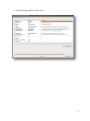
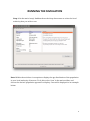
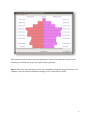
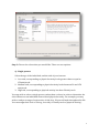
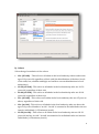
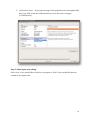
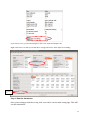
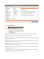
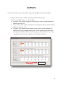
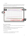
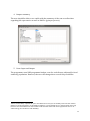
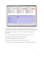
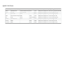
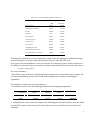
Physical Activity Tool User Guide: PAT4LG, Version 1.0 7 Contents BACKGROUND ............................................................................................................................................................................. 2 INSTALLING THE PROGRAM ............................................................................................................................................... 3 RUNNING THE SIMULATION ............................................................................................................................................... 5 OUTPUTS..................................................................................................................................................................................... 14 REFERENCES ............................................................................................................................................................................. 20 1 BACKGROUND Physical inactivity is considered as one of the four main behavioural risk factors which increase the risk of several non-communicable diseases (NCDs) (World Health Organization, 2011). Increasing the level of physical activity in a population reduces the risk of NCDs and delays the progression of some diseases. This physical activity tool will enable the user to test the impact of different scenarios. For example, what are the health and cost impacts if all individuals in a given population meet the recommendations for physical activity? Aims: 1. To project the incidence and prevalence of physical inactivity-related chronic diseases forward to 2035. The diseases included are coronary heart disease (CHD), stroke, hypertension, type 2 diabetes, breast and colon cancers, depression and dementia. 2. To estimate the costs avoided of these diseases to the National Health Service (NHS) following interventions which increase physical activity. A reference list of the data included in the model is outlined in appendix 1. 2 INSTALLING THE PROGRAM Step 0: Use a windows computer Step 1: Double click on the zip file called S64paTool.zip Step 2: unzip the S64paTool.zip folder and select ‘extract all’ (rf_pa_packfile.txt, UserGuides folder and S64Tool.exe) into a new folder Step 3: Right click on the file S64Tool.exe and run as an administrator. A first window pops up saying where: “deploying to the file path where the user is using the tool”. Click on “OK” Step 4: The user will need accept the terms and conditions of the tool to be able to use it on their system Step 5: Two events occur: 1. A file called LAsetup.nhf as well as five folders called: diseases, output, pdfs, S64Data and UserGuides are created 3 2. The following interface can be seen: 4 RUNNING THE SIMULATION Step 1: On the main ‘setup’ dashboard use the drop down menu to select the local authority that you wish to run. Note: Within the tool there is an option to display the age distribution of the population in your local authority of interest. To do this select ‘view’ in the main toolbar, and choose the desired ‘population pyramid’ to display. Cornwall is displayed as an example below: 5 This shows the total number of males and females in the local authority of interest and how they are distributed by age throughout the population. Step 2: Select the start and stop year for the simulation using the drop down menu. For example, you can run the simulation starting in 2015 and end it in 2030. 6 Step 3: Choose the cohort that you would like. There are two options: a) Single person: Select the age of the individual, and the risk of your interest: 1. Low risk, corresponding to physical activity levels greater than or equal to 150min/week 2. Medium risk, corresponding to physical activity levels between 30 and 150 min/week 3. High risk, corresponding to physical activity less than 30 min/week You may wish to select a single person, rather than a cohort, in order to determine the risk of disease to an individual from reduced physical activity. For example, you may wish to analyse a range of trajectories of risk for a 20-year old male throughout his life. You can assign their level of risk e.g. low risk (>150min/week of physical activity). 7 b) Cohort Select the age boundaries of the cohort: 18+ (all risk) – This refers to all adults in the local authority who are above the age of 18 years old, regardless of their risk (the distributions of the three levels of the risks, low, medium and high, are based on current distributions in local authorities) 18-39 (all risk) - This refers to all adults in the local authority who are 18-39 years old, regardless of their risk 40-64 (all risk) - This refers to all adults in the local authority who are 40-64 years old, regardless of their risk 65+ (all risk) - This refers to all adults in the local authority who are 65 years or above, regardless of their risk 18+ (at risk) - This refers to all adults in the local authority who are above the age of 18 years old and are ‘at risk’. ‘At risk’ is assumed to be individuals who are inactive individuals (<150 minutes/week) 18-39 (at risk) - This refers to all adults in the local authority who are 18-39 years old and are ‘at risk’. ‘At risk’ is assumed to be individuals who are inactive individuals (<150 minutes/week) 8 40-64 (at risk) - This refers to all adults in the local authority who are 40-64 years old and are ‘at risk’. ‘At risk’ is assumed to be individuals who are inactive individuals (<150 minutes/week) 65+ (at risk) - This refers to all adults in the local authority who are 65 years old or above and are ‘at risk’. ‘At risk’ is assumed to be individuals who are inactive individuals (<150 minutes/week) Note: You can also specify the gender of the cohort (it is set to analyse both females and males by default, but you can specify the programme to only produce outputs for a particular gender). If a cohort is selected the single person attributes are automatically set to Not required. Step 4: Interventions Select the intervention that you would like to test. For physical activity you can select one of the following interventions: 1. ‘No change’ – trends continue as expected with no intervention i.e. baseline 2. ‘All become active’ – everybody in the population moves in to the active category (≥150 mins/week of physical activity on a weekly basis) 9 3. ‘% becomes active’ - A given percentage of the population becomes physically active e.g. 25% of inactive individuals move in to the active category (>150mins/wk) Step 5: allow input cost editing Select ‘true’ if you would like to edit the cost inputs or ‘false’ if you would like them to remain as the input costs. 10 If you choose ‘true’, you should navigate to the ‘costs: Input and Output’ tab. Right click on the cost that you would like to change and select ‘Allow Input Cost editing’. Cost: Input and Output tab Step 6: Run the simulation Once you are happy with the set up, click ‘run cohort’ on the main setup page. This will run the simulation. 11 Step 7: THE MENU BAR The menu bar There are a number of additional features that can be selected from the menu bar: File/make data pack – this is restricted for the developer’s access only. Edit/setup - once you have run the simulation you can go back to the initial set up page by selecting ‘edit/setup’ Edit/clear output - once you have run the simulation this will delete all of the outputs from any previous runs you have done Run/initialise run - this gives you an overview of the initialisation components that you specified in the previous 4 steps above Run/run cohort – this runs the simulation in the same way as the ‘run cohort’ button on the main setup screen View/population tree – this allows you to view the population distribution of all ages, or specific age groups in the selected local authority 12 View/draw disease prevalence by year – selecting this with bring up a graph of the disease prevalence View/draw cost savings by year View/draw cumulative cost savings by year Help – this contains the user guide, glossary of terms and the method used for deriving costs 13 OUTPUTS Once the tool has run, there should be output tabs along the bottom of the page: 1. ‘Output: Counts’ tab – click the tab at the bottom of the screen. The user should be able to see three tables: ‘Baseline’: The number of people surviving in the cohort and the number of disease cases by year ‘Intervention’: The number of people surviving in the cohort and the number of disease cases by year ‘Changes’: The changes in the numbers in the cohort and the numbers of disease cases by year. Right clicking on a specific disease in this table and selecting ‘Draw Selected Disease [cases by year]’ will enable the user to plot changes in this disease for each year of the model simulation. Output: counts 14 2. Graphics This graph shows the year along the x-axis and the probability of being alive and having a disease on the y-axis. The diseases are listed at the top of the graph with average number of expected disease days per person throughout their life. Baseline Intervention Disease days Probability of having the disease Year Output How to interpret the graph: At baseline, the average number of disease exposure days for hypertension is 2162 and diabetes is 590 per person. Following the intervention, (all become active), the average number of disease exposure days for hypertension is 2129 and diabetes is 563. You can ‘right click on this graph’: This allows you to: - cycle graph mode – to cycle through different types of graphics - increase or decrease the precision of the y-axis 15 - save the graph as a jpeg file to use the pictures in your reports - take out diseases so that you can view other diseases on a more readable scale. 3. Output: life, death, disease The user should be able to see two tables: ‘Baseline cohort’: The annual mean probability of being alive and to have a disease or to die ‘Cohort post intervention’: The annual mean probability of being alive and to have a disease or to die 16 4. Output: summary The user should be able to see a table with the summary of the run as well as data regarding life expectancies as well as DALYs1 (gain per person). 5. Costs: Input and Output The programme uses NHS programme budget costs for each disease, adjusted for local authority population. However, the user can change these costs if they would like. 1DALYs are disability adjusted life years. One DALY is one lost year of "healthy" life. The sum of these DALYs across the population, or the burden of disease, can be thought of as a measurement of the gap between current health status and an ideal health situation where the entire population lives to an advanced age, free of disease and disability. 17 All the outputs are saved in the output folder under the local authority and time and date of the run. The counts by year can be found in the text file called: BaseCounts.txt The prevalence of the baseline scenario can be found in the text file called in BasePrev.txt The costs for the baseline and intervention by year can be found in Costs.txt The change in costs by year can be found in DiffCounts.txt The intervention costs can be found in IntCounts.txt The prevalence for the intervention can be found in IntPrev.txt The summary of the run (DALYs, life expectancy etc.) can be found in summary.txt 18 19 REFERENCES World Health Organization. (2011). Global status report on noncommunicable diseases 2010. Retrieved from http://whqlibdoc.who.int/publications/2011/9789240686458_eng.pdf 20 Appendix 1. Data references Diseases Incidence Prevalence Depres s i on computed from preva l ence Adul t Ps ychi a tri c Morbi di ty Survey, 2007 non-fa ta l Dementi a Ra i t et a l , 2010 CHD Smol i na et a l , 2013 Di a betes Pers ona l communi ca ti on Dr. Cra i g Curri e IDF 2012 Stroke BHF 2009 Hypertens i on computed from preva l ence Brea s t ca ncer Col orecta l ca ncer Survival Mortality Health care Costs Social care costs Utility weights RR physical activity non-fa ta l NHS Engl a nd, 2013 NHS Engl a nd, 2013 Hunter et a l ; 2013. US Surgeon Genera l Report, 2008 Al zhei mer's Soci ety, 2014 computed from prevaONS l ence 2013 a nd morta l i NHS ty Engl a nd, 2013 NHS Engl a nd, 2013 Sul l i va n et a l , 2011 Bl ondel l et a l , 2014 BHF 2014 computed from prevaONS l ence 2013 a nd morta l i NHS ty Engl a nd, 2013 NHS Engl a nd, 2013 Sul l i va n et a l , 2011 Li a nd Si egri s t, 2012 non-fa ta l NHS Engl a nd, 2013 NHS Engl a nd, 2013 Sul l i va n et a l , 2011 Jeon et a l , 2007 BHF 2014 computed from prevaONS l ence 2013 a nd morta l i NHS ty Engl a nd, 2013 NHS Engl a nd, 2013 Sul l i va n et a l , 2011 Li a nd Si egri s t, 2012 BHF 2012 non-fa ta l non-fa ta l NHS Engl a nd, 2013 NHS Engl a nd, 2013 Sul l i va n et a l , 2011 Hua i et a l , 2013 CRUK 2011 ONS 2012 CRUK 2012 NHS Engl a nd, 2013 NHS Engl a nd, 2013 Sul l i va n et a l , 2011 Lee et a l , 2012 CRUK 2011 ONS 2012 CRUK 2012 NHS Engl a nd, 2013 NHS Engl a nd, 2013 Sul l i va n et a l , 2011 Wol i n et a l , 2011 non-fa ta l Appendix 2. Glossary of terms Baseline – This refers to the ‘steady state’ of the risk factor. A scenario where no intervention occurs and trends continue unabated. Data pack - This is a single file which contains all of the disease and population statistics required by the tool. Disease exposure – this refers to the number of days per person that an individual has a disease. For example, 500 diabetes days refers to the number of days an individual is alive and lives with a disease Distribution –the frequency of various outcomes in a sample population. The frequency or count of the occurrences of values within a particular group or interval, and in this way, the table summarizes the distribution of values in the sample. Incidence – the occurrence of new cases of the disease – not to be confused with prevalence. Prevalence – this is the total number of cases of a disease in a particular population. This indicates how widespread the disease is. Probability – this is the chance of a disease occurring. Probability always lies within 0 and 1. Simulation – the imitation of a real-world process or system over time, in this case the simulation of a virtual local authority population Appendix 3. How are costs calculated? Cost data were taken from National Health Service programme Budget costs (NHS Networks, 2014). Both direct health care costs and NHS social care costs were extracted for each disease. When only total costs for a disease group were available (e.g. total cost of upper-gastrointestinal cancers) the cost of an individual disease within that group was calculated as a proportion of the total costs based on Hospital Episode Statistics (Health and Social Care Information Centre, 2014a; Health and Social Care Information Centre, 2014b). It was assumed that the costs for each disease in that group are equal. For example, for upper gastro-intestinal cancers we included oesophageal, stomach, small bowel, pancreas, liver and biliary cancer. To find out the costs of oesophageal cancer we divided incidence of oesophageal cancer by total hospital episodes of gastro-intestinal cancers and then multiplied the output by the total expenditure on gastro-intestinal cancers. For hypertension, outpatient cases only were used to estimate the ratio for the NHS budget costs. Inpatient data were excluded since hypertension patients are most likely to be seen within primary care and outpatient settings. For hypertension, outpatient cases only were used to estimate the ratio for the NHS budget costs. Inpatient data were excluded since hypertension patients are most likely to be seen within primary care and outpatient settings. Input costs – based on NHS programme budget costs Costs in £billion NHS Social care Hypertension 0.3294 0.0311 Coronary heart disease 1.4635 0.1343 Stroke 0.6757 0.1434 Diabetes 1.151 0.2306 Breast cancer 0.4477 0.0352 Colorectal cancer 0.3168 0.0297 Larynx cancer 0.0179 0.0038 Liver cancer 0.0265 0.0027 Oesophageal cancer 0.0518 0.0054 Oral and pharynx cancer 0.0569 0.0121 Liver disease/liver cirrhosis 0.0716 0.0037 Following the simulation run, the programme simply scales the aggregated individual disease costs according to the relative disease prevalence in years after the start year. In any year, the total healthcare cost for the disease D is denoted CD(year). If the prevalence of the disease is denoted PD(year) we assume a simple relationship between the two of the form CD year PD year for some constant . Since these costs are based on NHS programme budget costs for the whole of the country, the costs are multiplied by a ratio of the Local authority population relative to the English population. For example, to derive the costs for Ealing, we 1. calculated a ratio for the Total Ealing population/Total England population: Populations Males Females Total England 26533969 27331848 53865817 Ealing 169844 169470 339314 Ratio 0.006299 2. multiplied this ratio by the total output costs following the simulation (these costs are based on total NHS costs for the country). Therefore the costs were scaled for the size of the local authority. 1