Download DigiFlow User Guide - damtp

DigiFlow User Guide
Version 1.2, October 2006
© DL Research Partners
2000 – 2006
Contents
1 Introduction .......................................................................................................................1
1.1 History..........................................................................................................................1
1.2 Key features..................................................................................................................1
1.3 User guide ....................................................................................................................2
2 Installation .........................................................................................................................3
2.1 Basic installation ..........................................................................................................3
2.2 Windows configuration................................................................................................3
2.2.1 Basic configuration ...............................................................................................3
2.2.2 Encapsulated PostScript configuration ................................................................4
2.3 Installation with framegrabber .....................................................................................5
2.3.1 Framegrabber installation....................................................................................5
2.3.2 Camera configuration ...........................................................................................5
2.3.3 Local security policy .............................................................................................5
2.3.4 Video capture configuration .................................................................................5
3 Basics ..................................................................................................................................7
3.1 Image Selectors ............................................................................................................7
3.2 Sifting...........................................................................................................................8
3.3 DigiFlow Macros .........................................................................................................8
3.4 Threads.........................................................................................................................9
4 Common dialogs ..............................................................................................................10
4.1 Open Image ................................................................................................................10
4.2 Save Image As............................................................................................................12
4.3 Sifting input streams ..................................................................................................12
4.3.1 Selector timing ....................................................................................................13
4.3.2 Selector region ....................................................................................................14
4.3.3 Matching intensities ............................................................................................17
4.4 Modifying output streams ..........................................................................................19
4.4.1 Setting output stream colour ...............................................................................20
4.4.2 File format...........................................................................................................20
4.4.3 First index ...........................................................................................................20
4.4.4 Resampling..........................................................................................................20
4.4.5 Save user comments ............................................................................................21
4.4.6 Encapsulated PostScript streams........................................................................21
4.5 dfc Help......................................................................................................................21
4.6 Code library................................................................................................................23
5 Menus ...............................................................................................................................25
5.1 File..............................................................................................................................25
5.1.1 Open Image .........................................................................................................25
5.1.2 Save As ................................................................................................................25
5.1.3 Run Code.............................................................................................................25
5.1.4 Edit Stream..........................................................................................................25
5.1.5 Merge Streams ....................................................................................................26
5.1.6 Live Video ...........................................................................................................27
5.1.7 Print View ...........................................................................................................35
5.1.8 Export to EPS......................................................................................................35
5.1.9 Close....................................................................................................................36
5.1.10 Exit ....................................................................................................................36
5.2 Edit .............................................................................................................................36
5.2.1 Copy ....................................................................................................................36
5.2.2 Zoomed Copy ......................................................................................................36
5.2.3 Properties............................................................................................................37
5.2.4 Coordinates.........................................................................................................39
5.2.5 Process again......................................................................................................43
5.2.6 Dialog responses.................................................................................................43
5.2.7 dfcConsole...........................................................................................................44
5.3 View ...........................................................................................................................46
5.3.1 Zoom ...................................................................................................................46
5.3.2 Fit Window..........................................................................................................48
5.3.3 Cursor .................................................................................................................48
5.3.4 Appearance .........................................................................................................49
5.3.5 Colour scheme ....................................................................................................49
5.3.6 Toggle colour ......................................................................................................51
5.3.7 Toolbar................................................................................................................51
5.3.8 Slaves ..................................................................................................................51
5.3.9 Threads ...............................................................................................................53
5.3.10 Pause all threads...............................................................................................54
5.3.11 Refresh ..............................................................................................................54
5.4 Create .........................................................................................................................54
5.5 Sequence ....................................................................................................................54
5.5.1 Animate ...............................................................................................................54
5.6 Analyse.......................................................................................................................57
5.6.1 Time information.................................................................................................57
5.6.2 Ensembles ...........................................................................................................69
5.6.3 Dye images..........................................................................................................71
5.6.4 Synthetic schlieren ..............................................................................................78
5.6.5 Particles ............................................................................................................101
5.6.6 Particle Tracking Velocimetry ..........................................................................113
5.6.7 Optical flow.......................................................................................................134
5.7 Tools ........................................................................................................................138
5.7.1 Recipe................................................................................................................138
5.7.2 Transform intensity ...........................................................................................139
5.7.3 Combine images................................................................................................145
5.7.4 Slave process....................................................................................................149
5.7.5 To world coordinates ........................................................................................151
5.8 Window....................................................................................................................153
5.9 Help..........................................................................................................................153
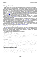
6 Techniques .....................................................................................................................154
6.1 Determining black....................................................................................................154
7 Chaining processes........................................................................................................156
8 Interpreter basics ..........................................................................................................159
8.1 Syntax.......................................................................................................................159
8.2 Variables ..................................................................................................................160
8.2.1 Simple variables................................................................................................160
8.2.2 Compound variables .........................................................................................160
8.3 Assignment...............................................................................................................160
8.4 Arrays.......................................................................................................................161
8.5 Lists..........................................................................................................................163
8.6 Operators ..................................................................................................................164
8.7 Constants ..................................................................................................................165
8.8 Execution control .....................................................................................................165
8.9 User-defined functions .............................................................................................166
8.10 User input and ouput ..............................................................................................168
8.11 Input from files.......................................................................................................168
8.12 Debugging ..............................................................................................................168
8.12.1 Error handling ................................................................................................168
8.12.2 View variables.................................................................................................169
8.12.3 Messages .........................................................................................................170
8.12.4 Queries ............................................................................................................171
8.12.5 Break points ....................................................................................................172
8.12.6 dfcConsole.......................................................................................................172
9 Functions........................................................................................................................175
9.1 Basic mathematical functions ..................................................................................176
9.2 String functions ........................................................................................................176
9.3 Information functions...............................................................................................176
9.4 Timing functions ......................................................................................................176
9.5 Type manipulation functions....................................................................................176
9.6 Statistical functions ..................................................................................................177
9.7 Image processing functions ......................................................................................177
9.8 Coordinate functions ................................................................................................177
9.9 Array plotting functions ...........................................................................................178
9.10 Numerical functions ...............................................................................................178
9.11 Differential functions .............................................................................................178
9.12 Flow functions........................................................................................................178
9.13 File handling...........................................................................................................178
9.14 Reading and writing images...................................................................................179
9.15 Windows and views ...............................................................................................179
9.16 Handling threads ....................................................................................................180
9.17 Logging ..................................................................................................................180
9.18 Camera control .......................................................................................................181
9.19 DirectDraw functions .............................................................................................182
10 Macros..........................................................................................................................184
10.1 DigiFlow command files........................................................................................184
10.1.1 Running processes...........................................................................................184
10.1.2 Accessing variables.........................................................................................185
10.1.3 Control of input streams .................................................................................186
10.1.4 Control of output streams ...............................................................................190
10.1.5 Chaining responses .........................................................................................193
10.1.6 Multiple output streams ..................................................................................194
10.1.7 Accessing dialogs ............................................................................................194
10.2 Recording user input ..............................................................................................195
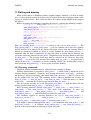
11 Plotting and drawing ..................................................................................................197
11.1 Drawing commands ...............................................................................................197
11.2 The DigiFlow Drawing format...............................................................................198
11.3 Simple plot .............................................................................................................198
12 Image file formats .......................................................................................................200
12.1 Windows bitmap files (.bmp).................................................................................200
12.2 TIFF files (.tif) .......................................................................................................200
12.3 GIF files (.gif) ........................................................................................................200
12.4 Enhanced metafiles (.emf) .....................................................................................200
12.5 Windows metafiles (.wmf).....................................................................................201
12.6 Encapsulated PostScript (.eps)...............................................................................201
12.7 DigiFlow floating point image format (.dfi) ..........................................................201
12.7.1 Header.............................................................................................................201
12.7.2 Tag ..................................................................................................................201
12.7.3 8 bit image (DataType = #1001).....................................................................202
12.7.4 8 bit multi-plane image (DataType = #11001) ...............................................202
12.7.5 Compressed 8 bit image (DataType = #12001)..............................................202
12.7.6 32 bit image (DataType = #1004)...................................................................203
12.7.7 32 bit multi-plane image (DataType = #11004) .............................................203
12.7.8 Compressed 32 bit image (DataType = #12004)............................................204
12.7.9 64 bit image (DataType = #1008)...................................................................204
12.7.10 64 bit multi-plane image (DataType = #11008) ...........................................204
12.7.11 Compressed 64 bit image (DataType = #12008)..........................................205
12.7.12 32 bit range (DataType = #1014).................................................................205
12.7.13 64 bit range (DataType = #1018).................................................................205
12.7.14 Rescale image (DataType = #1100) .............................................................206
12.7.15 Rescale image rectangle (DataType = #1101) .............................................206
12.7.16 Colour scheme (DataType = #2000) ............................................................207
12.7.17 Colour scheme name (DataType = #2001)...................................................207
12.7.18 Colour scheme name variable (DataType = #2002) ...................................207
12.7.19 Description (DataType = #3000)..................................................................207
12.7.20 User comments (DataType = #3001)............................................................208
12.7.21 Creating process (DataType = #3002) .........................................................208
12.7.22 Image time (DataType = #3018)...................................................................208
12.7.23 Image coordinates (DataType = #4008).......................................................208
12.7.24 Image plane details (DataType = #4108) .....................................................209
12.8 DigiFlow Particle tracking format .........................................................................209
12.9 DigiFlow pixel data format (.dfp) ..........................................................................209
12.10 DigiFlow drawing format (.dfd)...........................................................................210
12.11 DigImage raw format (.pic)..................................................................................210
12.12 DigImage compressed format (.pic).....................................................................211
12.13 DigImage movie format(.mov) ............................................................................212
13 Configuration files ......................................................................................................214
13.1 DigiFlow_LocalData.dfc........................................................................................214
13.2 DigiFlow_Configuration.dfc..................................................................................215
13.3 DigiFlow_Cameras.dfc ..........................................................................................215
13.4 DigiFlow_GlobalData.dfc......................................................................................218
13.5 DigiFlow_Phrases.dfr ............................................................................................218
14 Extending DigiFlow ....................................................................................................219
14.1 Installing extensions...............................................................................................219
References .........................................................................................................................220
Bibliography .....................................................................................................................220
Index..................................................................................................................................226
15 Licence Agreement......................................................................................................231
Licence: ..........................................................................................................................231
Warranty:........................................................................................................................232
Other Conditions: ...........................................................................................................232
DigiFlow
Introduction
1 Introduction
DigiFlow provides a range of image processing features designed specifically for analysing
fluid flows. The package is designed to be easy to use, yet flexible and efficient. Whereas
most image processing systems are intended for analysing or processing single images,
DigiFlow is designed from the start for dealing with sequences or collections of images in a
straightforward manner.
Before installing or using DigiFlow, please read the Licence Agreement (see §15) and
ensure you have completed the registration requirements.
1.1 History
The origins of DigiFlow lie in an earlier system by the same author: DigImage. This earlier
system, with its origins in 1988 and first released commercially in 1992, pioneered many uses
of image processing in fluid dynamics. Utilising its own DOS-extender technology, DigImage
existed in the base 640kB of DOS memory (and later from the command prompt under
Windows 3.x and 9x), accessing around 12MB of extended memory for image storage and
interface with the framegrabber hardware.
To obtain the necessary performance in these early days of image processing on desktop
computers, DigImage required a framegrabber card to be installed to provide not only image
capture, but also image display and some of the processing. While this close coupling allowed
efficient real-time processing and frame-accurate control of a video recorder, it ultimately
restricted the development and deployment of the technology. The original ISA bus based
Data Translation DT2861 and DT2862 frame grabber cards remained available until 2001, but
by that time suitable motherboards had become difficult to source. At time of writing (2004),
DigImage is still used in many laboratories around the world.
The development of DigiFlow began in 1994, although the project had a number of false
starts and development put on hold a number of times due to other commitments. The code of
this version has its origins in 1997 as part of the development of synthetic schlieren (see
§5.6.4). The computational and resolution requirements for synthetic schlieren could not be
accommodated efficiently within the framework of DigImage.
Despite sharing many approaches, algorithms and techniques, DigiFlow does not re-use
any of DigImage’s 8Mbytes Fortran 77 and 2MB Assembler source code. The design goals for
power, flexibility and efficiency in DigiFlow could only be achieved by starting again from
scratch.
DigiFlow builds on experience with DigImage from the user view point to provide a more
powerful, more flexible, but simpler interface. It also builds on the programming experience
to provide a more flexible, powerful and maintainable code base.
Versions of DigiFlow have been in use in Cambridge since 2000, and at other selected
laboratories since 2002. Its wider dissemination began in late 2003 with a series of beta
releases. The first commercial release (version 1.0) dates from February 2005.
1.2 Key features
DigiFlow has been designed from the outset to provide a powerful yet efficient
environment for acquiring and processing a broad range of experimental flows to obtain both
accurate quantitative and qualitative output.
Central to design philosophy is the idea that an image stream may be processed as simply
as a single image. Image streams may consist of a sequence of images (e.g. from a ‘movie’),
or a collection of images related in some other manner.
–1–
DigiFlow
Introduction
Efficiency is obtained through the use of advanced algorithms (many of them unique to
DigiFlow/DigImage) for built in processing options.
Power and flexibility are obtained through an advanced fully integrated macro interpreter
providing a similar level of functionality to industry standard applications such as MatLab.
This interpreter is available to the user either to directly run macros, or as part of the various
DigiFlow tools to allow more flexible and creative use.
Although not an essential component, DigiFlow retains the potential DigImage released by
the control of a framegrabber. Not only does this greatly simplify the process of running
experiments, acquiring images, processing them, extracting and plotting data, but it also
enables real-time processing of particle streaks and synthetic schlieren.
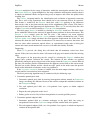
1.3 User guide
This User Guide is designed to provide the primary reference for DigiFlow. The User
Guide is supplied in both .html and .pdf formats and is linked to the help system within
DigiFlow. Pressing the F1 function key within DigiFlow will start a web browser and take you
to the most appropriate point in the .html version of the User Guide.
The User Guide is not in itself complete: detailed descriptions of the many functions
provided by the macro interpreter may be found in the interactive help system (Help: dfc
Functions). The User Guide is also supplemented by a variety of scientific publications that
expand on some of the underlying technologies.
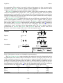
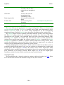
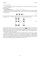
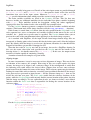
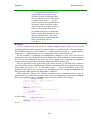
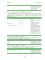
The typographical convention used in the User Guide is described below:
Typography
Analyse
Expt_A.mov
read_image
:=
"string"
# comment
my_image
file0
Description
Windows elements such as prompts, menu
items and dialogs.
File names, etc.
Interpreter commands and functions.
Interpreter operators and syntax.
Interpreter operators and syntax.
Formal argument names for interpreter
functions.
Variables, numbers, etc., for the interpreter.
Formal argument names for interpreter
functions.
–2–
DigiFlow
Installation
2 Installation
2.1 Basic installation
DigiFlow is a typical Windows application with a graphical user interface, menus, dialog
boxes and toolbars. However, unlike many applications, DigiFlow does not require a special
installation procedure, but can simply be copied to the desired directory. In most cases
DigiFlow will be delivered in a .zip file, downloaded from the web. This should simply be
unzipped into your selected directory. As such, DigiFlow does not require administrative
access to install.
The installed part of DigiFlow consists of DigiFlow.exe which contains the core
functionality, and a range of DLL files that handle specific menu options. DigiFlow also
makes use of various global start-up files stored in the same directory.
During use, DigiFlow generates two status files in the directory in which it is started. These
are DigiFlow_Status.dfs, which contains a range of information describing the settings, and
DigiFlow_Dialogs.dfs, which records your last responses to many of the prompts, etc. By storing
this information in the directory in which DigiFlow is started, DigiFlow is able to keep a
separate set of information for each user, or for each specific task, without polluting the
registry. Additionally, these status files can be deleted or moved as the user wishes. In some
circumstances, DigiFlow_Status.dfs may become corrupted. If DigiFlow fails to start, or exhibits
unexpected behaviour, you should try removing (or renaming) DigiFlow_Status.dfs to see if this
cures the problem.
It is recommended that you use a new directory for each new set of experiments and for
each new project. In this way the DigiFlow strategy of storing localised status files will
facilitate use of DigiFlow in the various different contexts. In such an environment it is
frequently most convenient to start DigiFlow from the command prompt within the
appropriate directory structure, although other strategies such as multiple shortcuts or setting
up associations for Windows Explorer are also possible.
If you wish to run DigiFlow from a command prompt (strongly recommended), it is worth
putting this directory on the path so that DigiFlow may be started by simply typing DigiFlow
at the prompt. If you prefer to start DigiFlow from the desktop or start menu, you will need to
create a shortcut at that point and set the Start in directory appropriately. It is strongly
recommended that you do not run DigiFlow from the directory in which the program resides.
2.2 Windows configuration
2.2.1 Basic configuration
Specification of the file extension for file names within DigiFlow is mandatory in most
circumstances as DigiFlow utilises this extension to determine the file type. However, by
default, Windows XP hides the extensions to files of known types, a feature that causes
problems with DigiFlow. We recommend, therefore, that you turn off this feature. This is
achieved through the View tab of Tools: Folder Options under Windows Explorer. Simply
remove the check mark from Hide extensions for known file types. Note that this will need to
be done for each DigiFlow user.
By default, DigiFlow will not be associated with any file types or extensions. If you wish to
make such an association (and thus allow DigiFlow to be started by double-clicking on a file
of that type within Explorer), then you should open Explorer and select View, Folder Options
then select the File Types tab. We recommend that the following extensions are associated
with DigiFlow on all installations: .dfc, .dfd, .dfi, .dft and .dfs. You may also wish to set up
associations for other standard image formats such as .bmp, .tif, .png and .jpg.
–3–
DigiFlow
Installation
2.2.2 Encapsulated PostScript configuration
DigiFlow can create Encapsulated PostScript (.eps) files from image and graphical output
for incorporation into documents in packages such as LaTeX and Word. This can be achieved
either through DigiFlow’s inbuilt .eps facility, or using a Windows printer driver. The former
is restricted to bit images (or a rasterised version of graphics), whereas the latter can produce
both bit image and vector graphics.
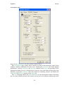
By default, DigiFlow searches for a printer named EPS to use to create the .eps files.
Creation of this printer is relatively straight forwards. Start the Add Printer Wizard from the
Printers and faxes window, selecting Local printer attached to this computer and using the
File: (print to file) port. Select a PostScript printer driver (e.g. the HP C LaserJet 4500-PS) and
name the printer “EPS”. (You do not want to make this the default printer, you may, however,
wish to share the printer to simplify the setting up of further machines.)
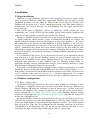
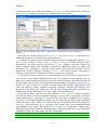
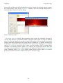
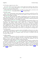
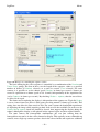
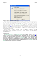
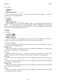
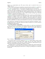
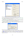
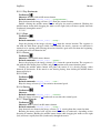
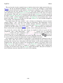
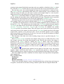
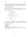
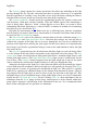
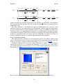
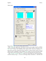
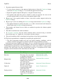
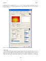
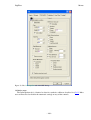
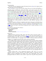
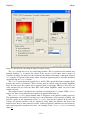
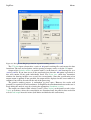
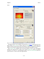
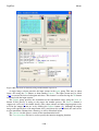
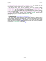
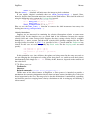
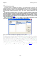
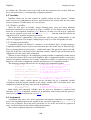
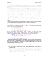
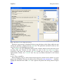
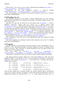
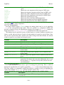
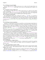
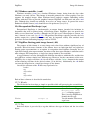
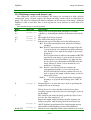
Once the wizard has finished, right-click on the new EPS printer and select Printing
preferences. Click on the Advanced button expand Document Options and PostScript
Options within it. Under PostScript Output Option select Encapsulated PostScript (EPS), as
indicated in figure 1.
Figure 1: Encapsulated PostScript (.eps) printer setup.
DigiFlow cannot itself read back in an Encapsulated PostScript file it produces. However,
if DigiFlow detects that GhostScript is installed on the machine, then DigiFlow will attempt to
use GhostScript to help it load the .eps file in an appropriate format. For this to be achieved,
then GhostScript must be on the system PATH and the GS_LIB environment variable must be
set up to point to the GhostScript libraries.
Note that GhostScript is not distributed with or required by DigiFlow. Use of GhostScript
is governed entirely by the licence of that product and not by the DigiFlow Licence.
–4–
DigiFlow
Installation
2.3 Installation with framegrabber
If you are installing DigiFlow in a machine equipped with a BitFlow R2, R3, R64 or R64e
series framegrabber then some additional steps are required. These require administrative
access to implement.
2.3.1 Framegrabber installation
The framegrabber should be installed and tested using the BitFlow installation procedure.
You will require the BitFlow drivers for version 4.00 or later.
The BitFlow framegrabber requires a configuration file (.cam, .rcl or .r64) for the camera
being used. Configuration files for cameras known to work with DigiFlow may be found at
http://www.damtp.cam.ac.uk/lab/digiflow/cameras/.
Once the framegrabber is installed, it is recommended that you use the Registry Editor
(regedit.exe; accessible from the command prompt) to adjust the permissions on all keys in the
registry relating to ‘BitFlow’ by adding the ‘Authenticated Users’ security principle with ‘Full
control’. Failure to do this would mean that only users with administrative access could
change the camera configuration.
2.3.2 Camera configuration
DigiFlow requires information about the camera capabilities and users preferences in order
to operate correctly. This information is stored in DigiFlow_Cameras.dfc; consult §12.2 for
details of the format of this file. Cameras not listed in this file have not been tested, although
there is a reasonable chance that all that is required is the addition of appropriate entries.
2.3.3 Local security policy
In the ‘Local security policy’ (found in the ‘Administrative tools’ section of the ‘Control
Panel’), open the ‘Local Policies: User Rights Assignment’ option. You need to add
permission for all DigiFlow users to the following items:
Adjust memory quotas for a process
Increase scheduling priority
Lock pages in memory
It is suggested that you do this by giving full control to ‘Authenticated users’
These adjustments are necessary to ensure that DigiFlow is able to manage the machine
performance adequately to ensure trouble-free capture.
2.3.4 Video capture configuration
It is strongly recommended that video capture is to a disk other than that containing the
operating system in order to obtain adequate performance. The necessary disk system
bandwidth may be in excess of 100MB/s in some cases (thus requiring a Mode 0 RAID array,
or using Windows to ‘stripe’ across multiple disks), but for most cameras 40MB/s is sufficient
and this may be achieved via a fast IDE or SATA disk (but not the one the operating system is
on!).
The capture process in DigiFlow can be configured in two ways. Either you can directly
specify the capture file and location each time (risking the user specifying a disk system with
insufficient bandwidth), or setting up DigiFlow to capture to a fixed location and require the
user to ‘review’ (and possibly edit) the sequence in order to copy it into their own directory
space. For multi-user systems, this second is generally preferred as it allows users to utilise the
capture facility like a video recorder while preventing retention of unwanted video footage.
The default configuration takes the second option, and assumes that the capture location is
V:\Cache\CaptureVideo.mov. We recommend that you configure your system so that this
–5–
DigiFlow
Installation
directory exists (either by appropriate naming of the capture disk, or by setting up a share to
an appropriate point and then connecting to it). This directory must not be compressed and
must have full access for all DigiFlow users. Once you have created this directory, you should
run File: Live Video: Setup (see §5.1.6.3 for further details) to create the initial
V:\Cache\CaptureVideo.mov. It is strongly recommended that you do this before writing any
other data to the capture disk. Details on how to change the name or location of the cache
file may be found in 13.1.
It is important that the space DigiFlow reserves in this file remains as a single contiguous
block on the disk drive. If it becomes fragmented for any reason then, due to the very high
data transfer rates required, DigiFlow may not be able to write to the disk as fast as data
becomes available from the camera and so timing errors may result.
Once created, V:\Cache\CaptureVideo.mov will be flagged as Read only by the operating
system (although DigiFlow will still be able to write to it). The file will not shrink if a smaller
sequence is captured, but may grow if one larger than that specified during File: Live Video:
Setup is requested (note that there is a risk of fragmentation if this occurs). It is important,
therefore, that you go through the review process outlined in §5.1.6.1, rather than simply
copying this file, as in general only a part of the file will contain valid data.
Consult §12.1 on DigiFlow_Configuration.dfc should you wish to change the name or location
of V:\Cache\CaptureVideo.mov.
–6–
DigiFlow
Basics
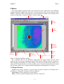
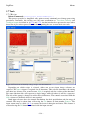
3 Basics
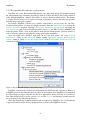
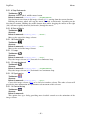
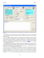
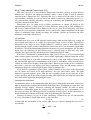
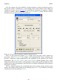
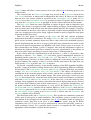
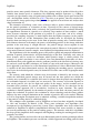
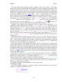
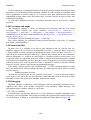
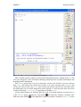
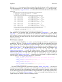
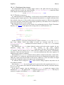
The main DigiFlow window follows that common for most applications with a Multiple
Document Interface (MDI). The menu bar at the top provides access to the majority of the
facilities, while the toolbar underneath gives a more convenient method of accessing the more
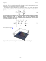
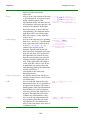
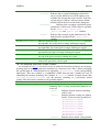
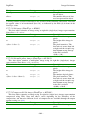
widely used functions. A typical example is shown in figure 1.
Toolbar
Menu Bar
Close
window
Image
window
Thread
running
indicator
Cursor
intensity
Resize
grip
Cursor
coordinates
Current
time
Thread
name
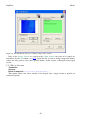
Figure 2: The basic DigiFlow window.
As is normally the case for Windows applications, the main window and the client
windows may be resized by dragging the frame of the window. Holding down the control key,
while dragging the boundary of a client window, will cause the contents of the window to be
zoomed so as to make the best use of the available space. If you do not hold down the control
key, then the window size is changed without changing the zoom applied to its contents.
3.1 Image Selectors
DigiFlow uses image selectors to specify image streams for input to and output from a
given process. Four types of image stream are supported:
Single images. These contain just a single image.
Movie. A movie contains multiple images stored in a single file.
–7–
DigiFlow
Basics
Sequence. A sequence is a collection of related files, typically identified by a numeric part
of the file name that increases by one between neighbouring images in the sequence.
Collection. A collection is a group of image files that have no special relationship to each
other. Collections may be subdivided into two groups: homogeneous collections and
heterogeneous collections. In a homogeneous collection, all the images within the collection
have the same format (same size, colour depth, file type, etc.). With a heterogeneous
collection, the format may vary from one image to another. At present, most processes within
DigiFlow do not support heterogeneous collections.
Image selectors may specify not only raster format image files, but also vector format files.
DigiFlow supports many standard raster formats, including .bmp, .tif, .gif, .png and .jpg, along
with special formats to provide backward compatibility with DigImage (.pic and .mov).
DigiFlow also introduces the new DigiFlow Image format, .dfi, to allow images to be saved
with full floating point precision, and the DigiFlow Pixel format (.dfp) provides text output
specifically tailored for raster images.
Vector format files include Enhance Meta Files (.emf) Windows Meta Files (.wmf) and
DigiFlow Drawing format (.dfd). The last of these provides output formatted as plain text
containing both data and drawing commands. This text may be imported into other
applications, or read back into DigiFlow to reconstruct the image or drawing it represents.
DigiFlow also provides a specialised file format (.dft) for storing particle tracking data.
While these may be treated as images, in general the functionality available through the
specialised particle tracking facilities is to be preferred.
The specialised DigiFlow and DigImage formats (.dfi, .dfp, dft and .dfd) are described more
thoroughly in §10.2.
3.2 Sifting
A key concept associated with input image streams is sifting. In DigiFlow, sifting is the
process by which images are extracted from in input stream. The extraction process may result
in all the images being extracted, or only a subset of images (typically specified by a start
number, an end number and a step). It may also result in a subregion of the image (a
rectangular window within the image) being returned, or, in the image being modified to
conform to some reference. Further details of the sifting process are given in §4.3.
3.3 DigiFlow Macros
DigiFlow includes a powerful interpreter and associated macro language. In the context of
these documents, segments of code or complete macros are referred to as dfc code. While the
programming language for dfc code is specific to DigiFlow, it follows the general syntax and
conventions of many other modern high-level languages. In addition to the basic functionality
expected of such languages, DigiFlow provides a vast array of functions tailored specifically
to tasks for which DigiFlow is ideal. This includes not only image processing functions
(ranging from contour tracing to Fast Fourier Transforms), and data analysis functions (such
as statistics, least squares fits), to numerical solution of the equations of motion (e.g. Goudnov
solution of shallow water equations and stream function-vorticity formulation for twodimensional Boussinesq flows).
This manual contains introductory documentation for the use of dfc functions and code.
However, much of the detailed documentation for the individual dfc functions is to be found
in the interactive help system Help: dfc Functions. The DigiFlow \macros\ directory contains a
number of documented examples of macro code.
–8–
DigiFlow
Basics
3.4 Threads
One important aspect of DigiFlow is that it supports not only multiple image windows, but
also multiple processing threads. This has two important benefits. First, it allows DigiFlow to
continue to be used interactively while it is processing simultaneously one or more sequence
of images, thus allowing real-time inspection of the progress. Second, for PCs with multiple
processors, the execution time of a single process can be greatly reduced. (It should also be
noted that more than one copy of DigiFlow may be used simultaneously).
If the user attempts to close a window that is in use with an active thread, then the system
will warn the user that closing the window will also kill the thread. Windows that are playing
a role in an active thread have the name of the thread indicated in the window status bar at the
bottom of the window and have a rotating
symbol in the bottom right-hand corner.
The user may also control the individual threads more directly, stopping them, pausing or
resuming them, or changing their priority. This is achieved through the View Threads menu
item (§5.3.7), or the corresponding
button on the main toolbar. (All active process threads
may be suspended by clicking on the toolbar.)
–9–
DigiFlow
Common dialogs
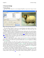
4 Common dialogs
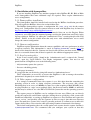
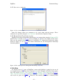
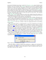
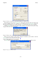
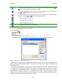
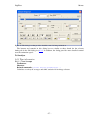
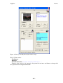
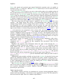
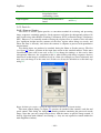
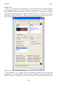
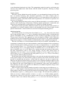
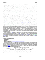
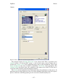
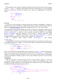
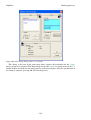
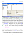
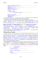
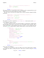
4.1 Open Image
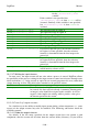
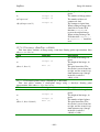
The Open Image dialog box is used throughout DigiFlow to open source image selectors
(§3.1).
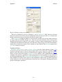
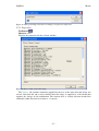
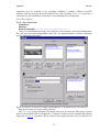
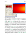
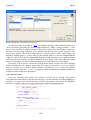
Figure 3: The Open Image dialog box.
The Open Image dialog box consists of a standard Explorer-style display of folders, files,
file types, etc., along with a preview pane on the right-hand side. This preview pane will
attempt to display the currently selected file.
DigiFlow supports a range of industry standard image formats, plus some special formats.
The special formats both provide compatibility with the earlier DigImage system, and provide
facilities (e.g. floating point data representation) not found in industry-standard formats. These
non-standard formats are described in more detail in §10.2 (DigiFlow drawing format) and
§11 (DigiFlow image file formats). Note that DigiFlow expects the user to specify the
extension of the file. It is therefore important that all extensions are visible in the dialog (refer
to §2.2 for how to achieve this).
To select a single image or a movie, simply click on the name of the file containing this
object. If you prefer, the name of the file may be typed at the File name prompt. If you type in
the file name a preview will not be generated automatically, but can be requested by clicking
the Preview button.
To select a sequence, the name of the sequence must be typed at the File name prompt,
using hashes (#) to indicate the varying numeric part of the file name. Alternatively, click on
any member of the sequence and check the Numbers as #### box. This will convert (starting
from the right-hand end of the file name) any digits found into the appropriate number of hash
characters, thus allowing easy specification of the sequence. Again, the Preview button may
be used to generate a preview if it is not generated automatically.
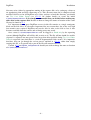
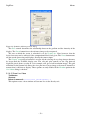
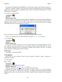
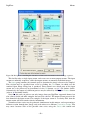
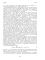
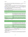
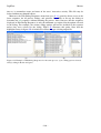
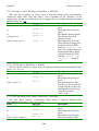
If you have a large number of numbered images in a given folder, the Compact list check
box will provide a more compact summary of those present by displaying the name of the first
few in a given sequence, and using the compact hash notation to summarise the rest. An
example of this is given in figure4. Selecting the summary containing hashes is equivalent to
– 10 –
DigiFlow
Common dialogs
selecting the entire series. (Note that clicking on Compact list will retain the files specified at
the Object name prompt, but remove any selection in the view window.)
Figure 4: The Open Image dialog using a compact list for summarising images belonging to a
sequence.
Note that the default settings of the Number as #### and Compact list check boxes is
remembered from one invication of the dialog to the next.
A collection of images may be specified using the mouse in combination with the <shift>
key to select a range of files, or the <ctrl> keys to select or deselect individual files.
Alternatively, the names may be typed at the File name prompt, each name enclosed by
double quotation marks. The collection is sorted into alphabetical order for display and
processing. (If a collection is specified in this manner then any hash characters will be
interpreted as hashes. Similarly, checking Number as #### will be ignored.) In general, a
sequence is preferable to a collection as it offers a greater level of control.
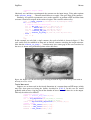
A collection of images may also be selected using wildcards. This may be achieved in two
ways. If you use the standard Windows wild cards (? to represent a single character, and * to
represent a variable number of characters) then the dialog will display only those files that fit
the description; you may then select them in the normal manner. Alternatively, you may use %
in place of ? and $ in place of * to do the selection directly. For example, typing Sheep*.* will
cause the dialog to display sheep2.tif, sheep.bmp, sheep.jpg, sheep.pic and sheep.tif to be
displayed in the dialog box, which may then be selected using the mouse and shift key.
Alternatively, Sheep$.$ will achieve the same result, selecting all five files.
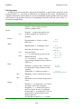
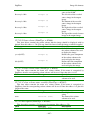
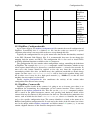
If the selected image contains true colour, then the Colour component list box is enabled.
This list box allows selection of whether the image is to be treated as full colour, or how the
colour information is converted to a greyscale for processing by DigiFlow. For example,
selecting RGB will allow DigiFlow to process the red, green and blue image planes separately
(where this makes sense), while green will take the green component of the colour image and
treat it as a greyscale image, or hue will process the colour using a hue/saturation/intensity
representation of the image. The options greyscale and mean all produce a similar effect,
although precise details of how the resulting image is constructed from the red, green and blue
components differs. The table below gives the relationships.
Key
RGB
Returns
Comments
Three colour planes
Full colour image
– 11 –
DigiFlow
red
green
blue
grey
mono
mean
max
min
Common dialogs
red
green
blue
0.11*red + 0.59*green + 0.30*blue
0.11*red + 0.59*green + 0.30*blue
(red + green + blue)/3
max(red, green, blue)
min(red, green, blue)
Red component only.
Green component only.
Blue component only.
Same as mono.
Same as grey.
Mean of three components.
The brightest component.
The darkest component.
4.2 Save Image As
The Save Image As dialog is essentially the same as the Open Image dialog (§4.1), but is
produced when the name of the output image selector (§3.1) is required.
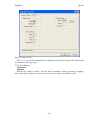
Figure 5: The Save Image As dialog box.
If an image selector of the same name does not exist already, then the file name must be
entered by typing at the File name prompt. The extension to be used should be specified
explicitly as DigiFlow uses this to determine the file type to be created. It is therefore
important that all extensions are visible in the dialog (refer to §2.2 for how to achieve this).
Simply selecting a type from the Save as type list will not necessarily have the desired effect
if more than one possible type is indicated.
Note that some file types have a range of options such as bit depth and compression. These
are normally controlled from outside the Save Image As dialog box using the Options…
button in the parent dialog. Refer to §4.4 for further details.
DigiFlow supports a range of industry standard image formats, plus some special formats.
The special formats both provide compatibility with the earlier DigImage system, and provide
facilities (e.g. floating point data representation) not found in industry-standard formats. These
non-standard formats are described in more detail in §10.2 (DigiFlow drawing format) and
§11 (DigiFlow image file formats).
4.3 Sifting input streams
When processing an image stream it is often desirable to select only a subset of the stream
for processing. This subset may contain only some of the images from the stream, and/or it
may contain only part of each image. Within DigiFlow this process of selecting a specific part
– 12 –
DigiFlow
Common dialogs
of an image stream for processing is referred to as ‘sifting’. When sifting is available, the
corresponding dialog will have a Sift… button (typically one for each input selector) that starts
a tabbed dialog box controlling the sifting process. The following subsections describe the
various sifting options.
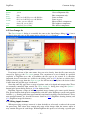
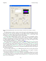
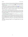
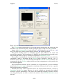
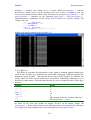
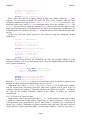
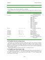
4.3.1 Selector timing
The Selector Timing tab of the Sift dialog allows the user to specify which times from a
multi-image image selector (§3.1) will be used for a process.
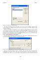
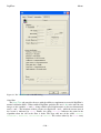
Figure 6: The standard Selector Timing tab of the Sift dialog.
This tab allows the preview of the image selector and specification of the processing start
and end points as well as the step between the images to be processed.
The buttons down the right-hand side allow the image selector to be played, the speed of
this preview controlled by the hare and tortoise buttons. The slider allows the currently visible
frame to be dragged to any time. The Frame edit box and spin control allow more precise
movement of the preview frame. The
and
buttons move to the currently specified limits
for the processing.
– 13 –
DigiFlow
Common dialogs
The frame numbers for the start and end points may be typed in the From and To edit
boxes, and the spacing in the Step edit box. The corresponding time boxes below will be
updated automatically.
Clicking the
buttons adjacent to the From or To edit boxes will set the corresponding
from or to position to the current position, shown by the slider and the edit boxes immediately
above (time) and below (frame).
Alternatively, holding <shift> while dragging the slider will allow specification of the
timings.
When the From and To times are set, or Step is not unity, then this information is displayed
on a yellow background at the top of the image preview.
For files that do not store timing information, the DigiFlow assumes by default that the
files are separated in time by one second. This may be changed using In file, in which the
image spacing may be specified in either seconds or, using the lower of the two controls, in
frames per second. These two controls are disabled for files that store time information, but
display the relevant details.
Reset to All resets the start and end points to include the entire selector.
Checking the Default colours control will cause the preview image to be displayed using
the DigiFlow default colour scheme rather than the colour scheme stored in the image file.
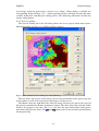
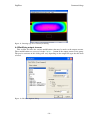
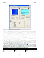
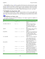
4.3.2 Selector region
The Selector Region tab of the Sift dialog allows the user to specify a region within an
image selector (§3.1) that will be used for a process.
– 14 –
DigiFlow
Common dialogs
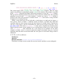
Figure 7: The standard Selector Region tab of the Sift dialog.
For a process requiring more than one input stream (and hence having more than one image
selector in its dialog box), one of the streams (typically the first in the dialog box) will be the
master stream. If the region for this stream is changed, then the region for the other (slave)
streams will be changed automatically to conform to (typically made the same as) that for the
master stream. It remains possible, however, to change independently the region for the slave
selectors, provided the size of the region for the slave selector is compatible with that for the
master selector.
The type of region is selected by the Region type group of radio buttons. The example
shown in figure 5 is for a master selector; the Conform option is not available here, but would
be visible above All when sifting slave selectors.
If Pixel window is selected, the pixel coordinates of the left, right, top and bottom of the
window may be specified in the edit controls within the black rectangle. If preferred, the size
may be increased without shifting the centre of the region, or the location of the region may be
changed without adjusting the size, using the Size and Position controls, respectively.
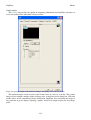
Alternatively, clicking the Draw button opens a full size window that allows the window to
be moved and resized dynamically using the mouse (see figure 6). The Zoom In and Zoom
Out buttons may be used to control the magnification while drawing. Similarly, you may swap
– 15 –
DigiFlow
Common dialogs
between this window and the Sift dialog box to use the various edit and spin controls to move
the region around. Click on the End Draw… button to close the drawing window and reenable the other controls on the Sift dialog.
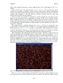
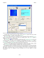
Figure 8: Drawing a region.
If Named region is selected, then previously saved regions are displayed and may be
selected. This provides a convenient method of using the same region in a range of different
processes. The four buttons to the right of the list box may be used to manage these named
regions. New named regions may be created either by clicking the New button, in which case
a subdialog is produced to allow specification of the region, or by clicking the Name button
(when Pixel window is selected) to give a name to a pixel window. The Edit button allows
alteration of an existing window, while Delete removes the region from the list. Note that
selecting a named region that is a Pixel window will update the controls in the Pixel window
group. Switching back to Pixel window allows editing of these values, while Name may be
used to overwrite the old values with the new ones, or to create a copy.
– 16 –
DigiFlow
Common dialogs
Figure 9: Editing a region.
4.3.3 Matching intensities
Quantitative measurements often require that the intensities are matched between different
frames and sequences. The intensities of the raw image streams may fluctuate due to a number
of reasons. One common one is the mismatch in frequencies between the illumination and the
camera frame rate. Depending on the type of light source and the shutter speed of the camera,
this mismatch may lead to a modulation of nearly 50% of the signal amplitude, while
automatic gain features can lead to similar results. While it is in general best to avoid these
problems by using continuous or high frequency light sources, this is not always practical.
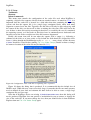
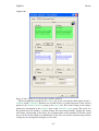
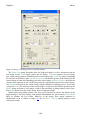
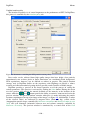
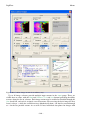
The Match Intensity tab in the Sift dialog (figure 8) provides a basic mechanism for
correcting the intensities of input image streams to match them to some fixed reference. The
basic strategy is for the image to contain two reference regions that contain approximately
uniform intensities that should not change with time. These two regions are then used to
generate a linear mapping between the input image and a reference intensity, thereby adjusting
the intensities in preparation for processing.
– 17 –
DigiFlow
Common dialogs
Figure 10: The Match Intensities tab provides the ability to directly relate an image to reference
values.
The Match Intensity facility is turned on and off using the radio button group in the topleft; .when off (None), then the intensities are read without alteration. The Match Intensity
facility can be enabled either using details provided locally (Local), or with details saved
previously (Named), in a similar manner to that used for Regions.
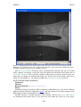
A locally defined Match Intensity reference consists of a pair of rectangular regions,
Region A and Region B. The location and size of these regions is controlled by a variety of
controls for specifying the left, right, top and bottom of each of the rectangles. Additionally,
as with the Regions dialog, the regions may be drawn on an image and dragged to their
desired location by clicking the Draw… button (see figure 9).
Each region requires an intensity to be associated with it. When Reference from is set to
Values, then the Intensity controls in the Region A and Region B groups is enabled. The user
may directly enter the desired (target) reference here, or by using File in Match to selector to
select a suitable image, then the Match button will read the intensities from the specified
image. Alternatively, if Reference from is set to First image, then the reference intensities are
not entered at this point, but rather they are determined automatically from the first image in
the stream to be processed.
Once the various controls for a Local Match Intensity have been set, their values may be
saved for use elsewhere by clicking Name…. This prompts for a user-supplied descriptive
name, saves the settings, and switches the dialog into Named mode.
Selecting an entry from Named matches loads the corresponding settings for use. If you
wish to alter the settings of a saved match, load it by selecting from the list, then switch to
Local mode. Make any necessary changes, then click again on Name to name and save it (you
may re-use an existing name).
– 18 –
DigiFlow
Common dialogs
Figure 11: Drawing regions for intensity matching.
4.4 Modifying output streams
This section describes the various modifications that may be made to the output streams.
These modifications are accessed via the Options… button in the output stream select group.
The precise contents of this dialog will vary depending on the output file type that has been
selected.
Figure 12: The Save Options dialog.
– 19 –
DigiFlow
Common dialogs
4.4.1 Setting output stream colour
The colour scheme for the output stream is selected from the list of known colour schemes
in the Colour scheme list box. Selecting the (input) member will set the colour scheme to be
the same as for the master input stream.
If you wish to add a new colour scheme or modify an existing scheme, you must use the
View: Colour Scheme… menu option. Refer to §5.3.5 for further details.
4.4.2 File format
The File format group invokes various options that may exist for the specified file type. The
contents of this group will depend on the file type specified: in many cases there are no
options and so the group is left empty.
The Bit depth field determines the number of significant bits saved for each pixel in the
image. Most image formats use 8 bits, but for high resolution images, or images that result
from numerical computations, a greater depth may be desired. If the .dfi format is specified for
the file type, then bit depths of 8, 32 and 64 bits are possible.
When available, the Compression level edit and spin control will determine whether or not
the image is to be compressed using a lossless compression. A value of zero indicates no
compression, with positive integers giving various levels of compression. Typically
compressing an image reduces its size by around a factor of two, but at the cost of slower
access (although for a very slow hard disk the access speed may improve with compression).
The additional time taken to compress an image will depend in part on the level of
compression requested, and in part on the structure of the image. If a process seems
particularly slow, but still producing the correct answer, try reducing the level of compression.
4.4.3 First index
By default, the first image in a sequence produced by DigiFlow will be given a zero index
(numerical part of the file name). The First index control may be used to change the index for
this first image. In either case, subsequent images will always be produced with unit
increments from this value.
4.4.4 Resampling
When the .dfi image format is selected, it is possible to rescale the output stream before it is
saved and then reverse this rescaling when the image is subsequently read in. Typically this
option is used to reduce the resolution of the saved image, but maintain its size by
interpolating back to the original size before using the image again.
This feature is enabled using the Resample check box. When enabled, the resolution of the
saved image is controlled by the Factor edit control which accepts a floating point value for
the relative resolution of the saved image. For example, a value of 0.5 will cause the saved
image to have only ¼ of the number of pixels of the original in the file, but through
interpolation the missing pixels are reconstructed when the image is read in again. This option
is particularly valuable for use with images produced by the synthetic schlieren (§5.6.4.3) and
PIV (§5.6.5.2) facilities.
– 20 –
DigiFlow
Common dialogs
4.4.5 Save user comments
Figure 13: User comments tab.
Some file formats allow user comments to be saved along with the images. These
comments are specified using the User Comments tab of the Save Options dialog.
4.4.6 Encapsulated PostScript streams
DigiFlow can produce Encapsulated PostScript (.eps) output either using the Export to EPS
option in the File menu (see §5.1.8) or by specifying an .eps file as the output stream. In the
latter case the normal Options dialog has an additional EPS button that invokes the dialog
shown in figure 14. See §5.1.8 for further information on the Encapsulated PostScript
formatting options.
Figure 14: The output options for Encapsulated PostScript (.eps) files.
4.5 dfc Help
As will be seen in §5, some of DigiFlow’s power and flexibility is gained by the use of
user-supplied macro code. This code is known as dfc code. Examples of facilities that require
such code include Analyse: Time: Extract (§5.6.1.4), Analyse: Time: Summarise (§5.6.1.5),
Tools: Transform Intensity (§5.7.2) and Tools: Combine Images (§5.7.3). Details of the macro
code itself are given in §§8 and 9. However, this manual gives only a relatively brief
– 21 –
DigiFlow
Common dialogs
introduction to a subset of the dfc functions available within DigiFlow. Instead, the bulk of the
documentation is provided within an interactive help facility available from within DigiFlow
itself in the Help: dfc Functions menu item, and from the
button within dialogs where such
information is of value.
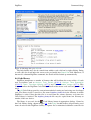
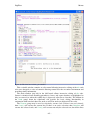
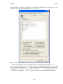
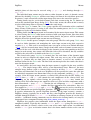
The help facility takes the form of the dialog illustrated in figure 15. To find a function
performing a given task, simply type some information about that task into the Search for
box. For example, if you want to find functions that have something to do with drawing, enter
“draw”. You will notice that as you enter “draw”, the Look up list changes as each letter is
typed. When you type the “d”, the size of the items in the list is reduced so that it only
includes those with a “d” somewhere in their names. Similarly, “dr” leads to a further
reduction, excluding those that do not have this pattern, and so on.
Spaces in the Search for box are interpreted as “and” criteria for the search. For example,
entering “dr ma” would reduce the list to those functions with both “dr” and “ma” in their
names, but without the two patterns needing to be adjacent. This, combined with the logical
and descriptive (if somewhat verbose) naming conventions for DigiFlow functions, provides a
very powerful search facility.
At all stages the Look up list is sorted alphabetically. (Note that if Search for is left blank,
then Look up contains all possible functions.)
Selecting an item in the Look up list then brings up the documentation for the function in
the three boxes below. The top of these identifies the role played by the entry within dfc code.
The list box below gives the range of possible entry points to the function. As we shall see
later, many DigiFlow functions are “overloaded” (i.e. they accept more than one type of data),
and may have optional parameters. This list itemises the full range of possibilities. Selecting
an entry point from this list and clicking the Copy button copies this entry point into the
clipboard.
The bottom control on the dialog provides the detailed documentation for the selected
function. This documentation should be read in conjunction with the entry point
documentation.
– 22 –
DigiFlow
Common dialogs
Figure 15: The help dialog for dfc code.
The help facility may also be started from within a code edit box by right-clicking. Doing
so will cause the word under the cursor to be pre-loaded into Search for field. Moreover, if
that word is a known DigiFlow command, the details will be looked up automatically.
4.6 Code library
DigiFlow incorporates a number of features that will facilitate the re-use of the dfc code
used in facilities such as Analyse: Time: Extract (§5.6.1.4), Analyse: Time: Summarise
(§5.6.1.5), Tools: Transform Intensity (§5.7.2) and Tools: Combine Images (§5.7.3). This
section describes the DigiFlow Code Library. Details of the macro code itself are given in §§8
and 9.
The dfc Code Library provides convenient method of storing and retrieving user-developed
code. The library itself is stored in a file named DigiFlow_Library.dfs in the directory in which
DigiFlow is started. Note that this file is re-read from the current directory every time the
Code Library is invoked. The DigiFlow_Library.dfs file may be copied from one directory to
another, if the user desires.
The library is accessed via the
Code Library button in appropriate dialogs. Central to
the Code Library dialog, shown in figure 16, is the Entry list that itemises all previously saved
items of code for this DigiFlow facility (a separate list is maintained within the same file for
– 23 –
DigiFlow
Common dialogs
each different facility). Any code currently specified in the parent dialog box is recorded under
the _current key; this will be the default selection upon entry.
To retrieve a previously stored code item, simply select it from the Entry list and click OK
to insert it in the parent dialog. The Code edit box will show the code, while Description will
show any previously saved description. Clicking Cancel will return to the parent dialog
without changing the code in that dialog.
Figure 16: The code library dialog.
The Code and Description may be edited before returning to the parent dialog.
Additionally, they may be saved back in the data base using the Save As button (see figure
17). The Delete button may be used to remove an entry from the Code Library, and the
button gains access to the dfc Help facility.
Figure 17: Name under which a Code Library entry is to be saved.
– 24 –
DigiFlow
Menus
5 Menus
This section describes the main menu options. Some of these will be familiar as they
follow standard Windows conventions, whereas others are specific to DigiFlow. Many of
these menu options can be strung together to create processes that are more complex. Details
of how to achieve this are given in §6.
5.1 File
5.1.1 Open Image
Toolbutton:
Shortcut: ctrl+O
Related commands: open_image(..), read_image(..), view(..)
Allows an image selector (§3.1) to be opened for viewing. The image is selected through
the Open Image dialog box (§5.1.2). Both images and drawing formats may be opened, but
not .eps Encapsulated PostScript.
5.1.2 Save As
Toolbutton:
Shortcut: ctrl+S
Related commands: save_image(..)
This option allows the contents of the active window to be saved. Note that if the active
window contains a sequence or other collection of images, only the currently displayed image
will be saved. To copy an entire sequence use File Edit stream (see §5.1.4) or one of the
related transformation tools.
5.1.3 Run Code
Toolbutton:
Shortcut: ctrl+R
Related commands: include(..)
Opens and runs a DigiFlow .dfc macro. Refer to §8 for further details.
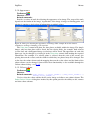
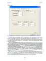
5.1.4 Edit Stream
Toolbutton:
Shortcut:
Related commands: process File_EditStream(..)
This option providesefficient editing of a single video stream.
– 25 –
DigiFlow
Menus
Figure 18: The Edit Stream dialog for editing a single video stream.
Parts of the Source Stream are copied to the Edited Stream; the parts to be copied are
determined by the Sift button (see §4.3). Typically this is used to change image file format,
reduce the time period, select only specific frames, and/or extract a subregion of the input
stream.
5.1.5 Merge Streams
Toolbutton:
Shortcut:
Related commands: process File_MergeStreams(..)
This option allows two video streams to be merged into a single stream to provide an
extended sequence.
– 26 –
DigiFlow
Menus
Figure 19: The Merge Streams dialog for combining image streams sequentially.
Two input selectors are provided: First and Second. These are written to the Output
selector in the order suggested by their names. The timings of the two input selectors need not
correspond, but the regions must conform. The First selector is the master, dictating the region
to be used.
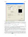
5.1.6 Live Video
5.1.6.1 Capture Video
Toolbutton:
Shortcut:
Related commands: process File_CaptureVideo(..)
Using this facility, a video sequence may be captured from one of the digital video cameras
supported by DigiFlow.
– 27 –
DigiFlow
Menus
Figure 20: Dialog box controlling the capture of video.
The basic timing for the video sequence is controlled by a combination of the Duration and
Frame Rates groups. The first of these sets the length of the sequence, either as a specified
number of frames (if Number selected), or as time in seconds (Time selected). For some
cameras, it is possible to set the shutter speed (Shutter, in frames per second; n frames per
second is equivalent to a shutter speed of 1/n seconds) independently of the acquisition rate
(set by Capture, in frames per second). By checking Shutter = capture, then the two of these
are forced to be equal.
The frame rate for updating the display is independent of the capture rate. Typically Display
is set to a lower frame rate (there is little point exceeding around 12 frames per second). This
setting does not affect the data stored to disk. For some systems the bandwidth requirements
of displaying the image while acquiring to hard disk exceeds that available. In such cases the
Display during capture check box should be cleared, thus suppressing the display during the
capture, although the display is still updated before capture begins and after capture finishes.
For some camera and framegrabber combinations, the raw data coming from the
framegrabber may not be in the correct format for display. This typically occurs with multi-tap
cameras; most single-tap cameras produce data in the correct format and require no additional
– 28 –
DigiFlow
Menus
processing. If additional processing is required, the Preprocess frame group determines what
should be done in this situation. The Untangle option forces the data to be untangled before
displaying or saving to hard disk. This option is the most processor and memory bandwidth
intensive, and so may not function adequately on all systems, especially during the capture
process when much of the bandwidth is already taken up. To overcome this, the Fast acquire
option untangles the images before and after the capture process, thus giving an intelligible
preview, but turns off the untangling during the capture. DigiFlow will automatically untangle
the image subsequently when it reads the image file produced in this manner. The remaining
option, None, turns off all processing.
The Display resolution group controls how much of the original image being captured by
the framegrabber will be displayed on the screen (note that this does not affect the data stored
to disk). The meaning of the various options is self-explanatory.
In some cases, simple real-time processing of the image prior to display will greatly assist
with the setting up and running of the experiment. The Display processing group controls the
type of processing that will be done. Note that this does not affect the data written to disk. To
suppress processing, select none from the list box. For large images, it may be best to use
Display resolution to reduce the resolution and thus the computational burden of undertaking
any processing.
The Output group provides a standard interface to select the destination for the captured
image. However, in some cases DigiFlow may be configured to always capture to a fixed
location (see §12.1 for details) to avoid the user having to select a disk drive with appropriate
characteristics and to force the user to go through a compulsory review process to extract only
those parts of the image stream that are of value. If this feature is enabled, then the Output
group will be disabled and following completion of the sequence capture, the Edit Stream
dialog (see §5.1.4) will be started automatically to control this second step. Not further that
DigiFlow can be configured to use a shared network drive for video capture. In this case, the
drive is locked during the capture process until the user has transferred the file off this server.
After pressing OK, DigiFlow opens an image preview, creates a Display processing dialog
(see below) if display processing was selected, and then prompts the user to start the
acquisition as illustrated in figure 11.
Figure 21: Message box starting the video capture.
After the sequence capture has finished, the performance is displayed in a message box,
such as shown in figure 13. The precise text in the message box will depend on whether or not
the compulsory review feature is enabled. Note that the ‘achieved’ timings may not be precise,
especially for relatively short sequences.
– 29 –
DigiFlow
Menus
Figure 22: Message box at end of video capture.
If the computer fails to keep up with the bandwidth requirements of the capture process,
then this will be indicated by there being some missed frames, and a lower than expected
frame rate being achieved. The amount of CPU time required is a strong function of any
display processing required. The synthetic schlieren option was selected for the example
illustrated in figure 13. This was performed on a 1GHz dual processor machine. Clearly more
CPU time was required than the capture time, but each processor was busy only around 60%
of the time. A single processor machine, however, would not have managed to keep up with
the bandwidth requirements.
Details subject to change. Currently works with BitFlow RoadRunner and R3
framegrabbers. Future possibilities are expected to include FireWire, Video For Windows
and TWAIN devices.
Particle Streaks
If Display processing is set to particle streaks then the dialog shown in figure 14 is
displayed to provide processing of display output while at the same time capturing the raw
video to a file. This dialog allows segmentation of the image into particles (bright points) and
background (dark points) by varying the Threshold control. Using relatively simple
processing, the particles so identified may be converted into comet-like streaks that slowly
fade with time. The length (in time) of these streaks is determined by the Length control. The
Reset button clears the display of all earlier times.
– 30 –
DigiFlow
Menus
Figure 23: Particle streaks preview dialog.
The rate at which the screen is refreshed is set by Display fps. Note, however, that the
desired rate may not be achieved if the computational load is too great. The Direct button turns
off the streaks processing and displays directly the camera input.
The Display step group of controls is used to aid the viewing of very large images that may
be larger than the available display area. The edit and spin controls set the step between
displayed pixels (hence a value of 2, for example, will give a half-resolution image). The grid
of buttons in the bottom left allows the view port into a larger image to be moved around in a
manner that is efficient to display. These options are only enabled if the Window option in the
Live Video dialog is checked.
Synthetic Schlieren
If Display processing is set to synthetic schlieren then the dialog shown in figure 15 is
displayed to provide processing of display output while at the same time capturing the raw
video to a file. This allows real time visualisation of a synthetic schlieren image (see §5.6.2).
There are three processing options: Difference is the simplest (and computationally fastest)
technique that provides a qualitative output proportional to the magnitude of the gradient in
the density perturbation. The Horizontal gradient and Vertical gradient options perform more a
more sophisticated analysis that returns a semi-quantitative output of the specified component
of the gradient in the density perturbation. Note that these two options distinguish between
positive and negative gradients.
– 31 –
DigiFlow
Menus
Figure 24: Synthetic schlieren preview dialog.
The Gain control determines the relationship between the gradient and the intensity of the
display. The Reset button forces the reference image to be recaptured.
The rate at which the screen is refreshed is set by Display fps. Note, however, that the
desired rate may not be achieved if the computational load is too great. The Direct button turns
off the streaks processing and displays directly the camera input.
The Display step group of controls is used to aid the viewing of very large images that may
be larger than the available display area. The edit and spin controls set the step between
displayed pixels (hence a value of 2, for example, will give a half-resolution image). The grid
of buttons in the bottom left allows the view port into a larger image to be moved around in a
manner that is efficient to display. These options are only enabled if the Window option in the
Live Video dialog is checked.
5.1.6.2 Show Live Video
Toolbutton:
Shortcut:
Related commands: process File_ShowLiveVideo(..)
This option creates a new window and streams live video directly to it.
– 32 –
DigiFlow
Menus
Figure 25: The dialog controlling what is seen in a live video window.
Video captured using this option is fed continuously to the display until stopped by the
user; it is not saved to hard disk. For this reason, no duration can be specified. For some
cameras, it is possible to set the shutter speed (Shutter, in frames per second; n frames per
second is equivalent to a shutter speed of 1/n seconds) independently of the acquisition rate
(set by Capture, in frames per second). However, many digital cameras force the two rates to
be equal.
The frame rate for updating the display is independent of the shutter and capture rates.
Typically Display is set to a lower frame rate (there is little point exceeding around 12 frames
per second). Any necessary processing of the incoming data stream to correct the format is
undertaken automatically.
The Display resolution group controls how much of the original image being captured by
the framegrabber will be displayed on the screen (note that this does not affect the data stored
to disk). The meaning of the various options is self-explanatory.
In some cases, simple real-time processing of the image prior to display will greatly assist
with the setting up and running of the experiment. The Display processing group controls the
type of processing that will be done. These are described in more detail for the Capture Video
option in §5.1.6.1. To suppress processing, select none from the list box. For large images, it
may be best to use Display resolution to reduce the resolution and thus the computational
burden of undertaking any processing.
– 33 –
DigiFlow
Menus
5.1.6.3 Setup
Toolbutton:
Shortcut:
Related commands:
This menu item controls the configuration of the cache file used when DigiFlow is
capturing a digital video sequence directly from an attached camera. As noted in §2.3.4, it is
important that the cache file is located on a disk other than that containing the operating
system, and that the capture file is in a single large contiguous block, rather than many
fragments scattered over the disk. Typically, the disk drive will only be able to keep up with
the camera if the drive can devote all its time to writing the video data. This will not be the
case if there is other disk activity occurring for that drive (as would be the case if it contained
the operating system), or if the heads of disk drive have to continually move backwards and
forwards across the disk as would occur if the file becomes fragmented.
Ideally, this menu item will be run when the capture disk is empty (e.g. following a
reformat of the disk) or at least nearly so. By default the disk should be assigned the drive
letter V: (either through the Disk Manager or by net use V: … onto a share) and the directory
V:\Cache should be created before running File: Live Video: Setup. (Details on how to change
the name or location of the cache file may be found in 13.1.)
Figure 26: Configuration of the cache file for capturing video sequences.
Figure 26 shows the dialog that is produced. It is recommended that the default size of
50GB is used. While this may seem excessively large, if you make the file too small you may
need to offload all your data and reformat the hard disk to be able to create a single large
contiguous file at a later stage.
Note that if DigiFlow detects an existing V:\Cache\CaptureVideo.mov, then this dialog will
not be produced. DigiFlow does not provide a mechanism for you to remove or change the
size of the cache file. If you must change the size, then you should delete it from Windows
Explorer then run File: Live Video: Setup again.
– 34 –
DigiFlow
Menus
5.1.7 Print View
Toolbutton:
Shortcut: ctrl+P
Related commands: print_view(..), ask_printer(..)
Print out the currently selected viewing window. The menu version of this facility produces
a dialog box allowing the user to select the printer, whereas the toolbar version simply prints
to the currently selected printer.
5.1.8 Export to EPS
Toolbutton:
Shortcut:
Related commands: export_to_eps(..)
Converts the currently selected viewing window into an Encapsulated PostScript (.eps) file.
Section 2.2.2 describes how to set up an .eps printer driver that allows both bit image and
vector graphics to be converted to .eps format. If the .eps printer is not set up, then DigiFlow
will convert vector graphics to a bit image before generating the .eps file.
When using the printer driver, not only can the user specify the name of the output file
(figure 27a), but some control over the format is also provided (figure 27b). In particular, a
title may be added either above or below the figure, and the figure may be given a frame.
Further, using the Text filter group, it is possible to suppress all text on a figure, or to replace
each element of text with a unique letter combination. These text filtering options are
provided for convenience with manuscript submissions where some journals wish all text
removed from figures, while others use systems such as the LaTeX \psfrag package to replace
the original text and fonts.
(a)
(b)
Figure 27: Exporting to an .eps file. (a) Selecting the output file. (b) Controlling the format of the
Encapsulated PostScript.
Note that .eps files may also be specified for the output stream from most of DigiFlow’s
menu options. If this is done, then the dialog in figure 27b replaces that normally produced by
the Options button.
– 35 –
DigiFlow
Menus
5.1.9 Close
Toolbutton:
Shortcut:
Related commands: close_view(..)
Close the active window. This is equivalent to clicking on the close button
left corner of the document window.
at the top
5.1.10 Exit
Toolbutton:
Shortcut:
Related commands: exit_digiflow(..)
Closes DigiFlow and all open image windows. This is equivalent to clicking on the close
button
at the top right corner of the main DigiFlow window. If DigiFlow detects that any
processes are currently running then it will prompt the user to ensure DigiFlow should still be
closed as this will terminate those processes.
5.2 Edit
5.2.1 Copy
Toolbutton:
Shortcut: ctrl+C
Related commands:
Copies the currently selected image or drawing to the system clipboard. The image or
drawing is available to other applications in both raster and metafile formats.
5.2.2 Zoomed Copy
Provides a group of options that allow images to be copied to the clipboard at a size that
differs from the full resolution image.
Double size
Copies the currently selected image to the system clipboard, doubling the size of the image
using bicubic interpolation, where appropriate.
Full size
Identical to Edit Copy (§5.2.1). Copies the currently selected image to the system
clipboard, doubling the size of the image using bicubic interpolation, where appropriate.
Half size
Copies the currently selected image to the system clipboard, halving the size of the image
first.
Copies the currently selected image to the system clipboard, reducing the linear resolution
of the image by a factor of three.
Quarter size
Copies the currently selected image to the system clipboard, reducing the linear resolution
of the image by a factor of four.
Zoom
Copies the currently selected image to the system clipboard, adjusting the resolution using
a user-specified factor (see figure )..
– 36 –
DigiFlow
Menus
Figure 28: Dialog selecting scale factor for image to be placed on clipboard.
5.2.3 Properties
Toolbutton:
Shortcut: ctrl+\
Displays the properties for the selected window.
Figure 29: Process that created the image.
The Process tab contains comments supplied by the user at the time when the image was
created. Note that this tab is only available when the image is supplied by a file format that
supports the storage of this information. The contents here is exactly that that invoked the
command (either interactively or from a .dfc macro).
– 37 –
DigiFlow
Menus
Figure 30: User comments.
The Notes tab contains comments supplied by the user at the time when the image was
created. Note that this tab is only available when the image is supplied by a file format that
supports comments.
– 38 –
DigiFlow
Menus
Figure 31: Image format.
The Format tab contains information describing the format of the image. This information
is available for all image types.
5.2.4 Coordinates
Toolbutton:
Shortcut:
Provides the ability to define, edit and delete coordinate systems providing a mapping
between the pixel coordinates of an image and some user-defined coordinate system.
– 39 –
DigiFlow
Menus
Figure 32: Selection of coordinate system.
The top-level dialog provides the ability to select the active coordinate system for the
current window by clicking on the desired entry in the list box, or to make changes to the
available coordinates.
The Edit, New and Copy buttons are used to adjust an existing coordinate system, create a
new coordinate system, or create a copy of an existing coordinate system (respectively). A
more complete description of these buttons is given below. The Delete button will remove the
currently selected coordinate system from DigiFlow, while Make Default will register the
selected system as the default for other operations.
5.2.4.1 New coordinate system button
To create a new coordinate system, click on New. This starts a dialog allowing the name,
type and units of the new coordinate system to be specified.
Figure 33: Give a name and type to the new coordinate system.
The Name of the coordinate system is arbitrary. The user should select a name that is
meaningful to the task at hand. This name will subsequently be used for identifying the
coordinate system. The Units are also arbitrary. They may refer to some standard measure of
– 40 –
DigiFlow
Menus
length, or to a dimensionless unit. The name of these units is recorded for later use in
captions, titles, etc.
There are three possible types of coordinate system that may be specified. Pixel coordinates
have a one to one correspondence with the pixels in the image and are the least flexible.
Function coordinates have a user-specified mapping between the pixel and user
coordinates. This form of mapping is the most precise, but will only be of use where there is
some external method of determining the required mapping functions. Four functions are
required, separated by semicolons. The first two functions give the world x and y coordinates
as functions of the pixel coordinates i and j, while the third and fourth give the pixel
coordinates as functions of the world coordinates.
Mapping coordinates are generally the most useful. These systems are specified through a
combination of mapping functions and identification points where both the pixel and user
coordinates are known. A least squares mapping is then used to generate the unknown
coefficients in the mapping functions and complete the transformation. There are a number of
pre-defined mapping functions, or the user may specify their own. The format of the mapping
function specification is an arbitrary name followed by a colon then a list of basis functions,
each separated by a semicolon and expressed in terms of the generalised coordinates x and y,
and optionally the time t. The points defining the unknown coefficients are specified using the
Edit button of the parent dialog.
5.2.4.2 Edit coordinate system button
The Edit button starts a dialog that may be used to edit the Units and Mapping functions for
the coordinate system. As noted above, the coordinate system may also be time dependent, in
which case Use Time-dependent Mapping should be checked and the points defining the
coordinate system should span both space and time.
Figure 34: Editing coordinate systems.
To specify the points used for the mapping, the Edit Points button should be clicked, which
will allow the user to specify points in the window that was active before entering the
coordinate system dialogs. At the same time a modeless dialog box, which should be used to
indicate the specification of the points is complete, is started.
Coordinate points are specified within the window by clicking at the desired location. This
places a plus mark (+) at the position. The plus mark may then be dragged to a new location,
if desired. Double-clicking the plus mark activates a dialog for specifying the user coordinates
for this point.
– 41 –
DigiFlow
Menus
Figure 35: World coordinates for a point when defining a coordinate system.
This dialog gives the current Pixel Position of the point (and allows this to be edited), and
provides the ability for the user coordinates to be defined in the World Position group. If a
time-dependent mapping were specified, then the Time for this point must also be specified.
Clicking Delete will remove the point, while checking Lock will prevent the point being
dragged around the image accidentally.
Figure 36: Indicate that you have finished editing the coordinate system markers.
When you have finished adding and/or editing the coordinate system markers, click the
Finished button in the dialog shown in figure 36.
5.2.4.3 Copy coordinate system button
The Copy button provides the ability to make a copy of an existing coordinate system.
Figure 37: Copy a coordinate system.
– 42 –
DigiFlow
Menus
5.2.5 Process again
Toolbutton:
Shortcut:
Related commands:
Users often wish to reprocess an image, perhaps making minor changes to the control
settings, or maybe to apply the same process to a different set of images. The Process again
facility provides a convenient method for doing this.
To use this feature, simply open the image for which you wish to replicate the process, and
click on the Process again button (or select from the Edit menu). DigiFlow will then recover
the process settings from the image and, where possible, use them to initialise the dialog that
was initially used to create the image.
Note that this feature only works with DigiFlow-specific formats such as .dfi, .dfd or .dft
files as other formats do not provide an appropriate mechanism for storing the settings used to
create the image.
5.2.6 Dialog responses
The purpose of this facility is to provide an aid for those trying to create .dfc files (see §8)
to run processes, and to provide an alternative user interface to many of the DigiFlow
processing facilities.
Figure 38: The Dialog Responses dialog that contains details of the responses corresponding to the
latest invocations of the dialogs.
The Process list box indicates the dialog for which responses are required. This list is
empty when DigiFlow is first started in a directory, but gradually fills as more DigiFlow
features are used. Upon exit from DigiFlow, all this information is saved in the
DigiFlow_Dialogs.dfs file that is created in the DigiFlow start directory.
– 43 –
DigiFlow
Menus
Selecting a dialog from the Process list causes the corresponding response lines to be
displayed in the Response variables edit box on the left-hand side of the dialog. Note that the
entries in this edit control are always displayed in alphabetical order, and the list will only
contain assignment statements. Entries in the edit box may be edited, selected, copied, etc., as
is standard for edit boxes. Users may find it useful to copy the contents of this edit box to .dfc
files they are creating.
If the responses variables are edited, then they may be saved by clicking Save; alternatively
Reset restores them to their previous values. The user will also be prompted to save any
alterations if a different dialog is selected from the list.
The corresponding dialog may be started (e.g. to provide updated values) by clicking the
Dialog button, while clicking Execute will cause the corresponding process to be started.
5.2.7 dfcConsole
Toolbutton:
Shortcut: ctrl+E
Related commands:
The dfcConsole provides an interactive tool for writing, editing and debugging dfc macro
code.
– 44 –
DigiFlow
Menus
Figure 39: The dfcConsole dialog is resizable.
This resizable window contains an edit control allowing interactive editing of the dfc code
to be run, alongside a series of controls allowing control over the execution environment and
providing timely information.
The main window (top left) in the dfcConsole allows interactive editing of dfc code.
Syntax is colourised and, matching parentheses, braces and square brackets are highlighted as
they are entered (or when the <shift> key is depressed adjacent to a bracket). The buttons in
the Code group down the right-hand side provide the basic editing functionality in
conjunction with standard short cuts such as ctrl+Z for undo (or shift+ctrl+Z for redo).
The Execute group may be used to selectively execute code. If there is no text selected,
then Line(s) will execute the current line. If there is an active selection, then Selection will
execute the selected code, and Line(s) will execute not only the selected text, but all the lines
– 45 –
DigiFlow
Menus
on which some text is selected. Regardless of the selection, All will cause the entire code to be
executed. Note that <alt><enter> is equivalent to clicking Line(s).
All the control buttons are disabled while the code is executing with the exception of Stop
in the Execute group. Clicking the stop button
will abort the currently executing code,
will temporarily suspend execution. Checking Breaks (&) causes
while the pause button
break points, indicated by an ampersand in the code (see §8.12.5) to be executed as and when
they are found by the interpreter. If cleared, then the break points are ignored. Note that the
status of the Breaks (&) control may be changed by the user as the dfc program runs.
The Interpreter group controls the internal state of the DigiFlow interpreter. Reset will
clear all variables and functions from the interpreter, while View displays the variables and
objects defined within the interpreter using the view_variables(..) interface. If an error
occurs, then Last Error will redisplay the last error message.
Below the code window is a documentation window. When DigiFlow detects a function
name under the cursor in the code window then it will display the documentation for this
function. This documentation (which is also accessible through the dfc help facility) is
hyperlinked to aid navigation. Standard forward and back navigation buttons are provided to
the right of the window.
The two windows at the bottom of the dfcConsole provide information about the contents
of variables. When the cursor is on a variable name, and that variable has a defined value
(typically the result of executing part of the code), then a summary of its contents will be
displayed. The window on the right displays the output resulting from a Query. See §8.12.4
for further details.
Note that using the Close button to close the window will prompt to save the dfc code it
contains, whereas using the x button will simply close the window without prompting for the
dfc code to be saved.
5.3 View
5.3.1 Zoom
5.3.1.1 In
Toolbutton:
Shortcut:
Related commands: view_zoom(..)
Zoom in the current window by a factor of two.
5.3.1.2 Out
Toolbutton:
Shortcut:
Related commands: view_zoom(..)
Zoom out the current window by a factor of two.
5.3.1.3 Full size
Toolbutton:
Shortcut:
Related commands: view_zoom(..)
Zoom the current window to full size (one pixel on the display for each pixel in the stored
image).
– 46 –
DigiFlow
Menus
5.3.1.4 Custom
Toolbutton:
Shortcut:
Related commands: view_zoom(..)
Starts the zoom dialog box that allows a broader range of zooms to be selected, and also
allows specification of the aspect ratio for the displayed image.
Figure 40: The custom zoom dialog box.
The two slider controls are linked with the two edit boxes. The Zoom setting controls the
number of pixels on the display used to display a single pixel in the stored image in the
horizontal direction. In contrast, the Aspect Ratio control determines the shape of the virtual
pixels to be displayed. For images captured through DigImage, the aspect ratio should be set
to 0.68 for PAL systems, or 0.75 for NTSC, thus recovering the original aspect ratio of the
images.
5.3.1.5 To Window
Toolbutton:
Shortcut:
Related commands: view_zoom_to_fit(..), view_zoom_all_to_fit(..)
Changes the zoom to fit the current window.
5.3.1.6 All Full Size
Toolbutton:
Shortcut:
Related commands: view_zoom_all(..)
Changes the zoom of all windows to 100%, and fits the windows to the size of the images.
5.3.1.7 All Half Size
Toolbutton:
Shortcut:
Related commands: view_zoom_all(..)
Changes the zoom of all windows to 50%, and fits the windows to the size of the images.
– 47 –
DigiFlow
Menus
5.3.1.8 All Third Size
Toolbutton:
Shortcut:
Related commands: view_zoom_all(..)
Changes the zoom of all windows to 33%, and fits the windows to the size of the images.
5.3.1.9 All Quarter Size
Toolbutton:
Shortcut:
Related commands: view_zoom_all(..)
Changes the zoom of all windows to 25%, and fits the windows to the size of the images.
5.3.2 Fit Window
Toolbutton:
Shortcut:
Related commands: view_fit_to_zoom(..), view_fit_all_to_zoom(..)
Resizes the current window so that it fits the zoom of its contents.
5.3.3 Cursor
Under all cursor modes, holding down the left mouse button will cause a duplicate cursor
to be displayed at the same pixel location on all the other open image windows. This feature is
valuable when trying to assess the relationship between features in different images. As
described below, the cursor can also be set to display other information or to perform other
tasks when the buttons are clicked.
5.3.3.1 Show Where
Toolbutton:
Shortcut:
When the left mouse button is held down on an image, a popup window will appear next to
the cursor showing the current pixel and (if defined) world coordinates. Clicking the right
button (while the left button is still depressed) will produce a message box showing the
coordinates.
5.3.3.2 Measure Distance
Toolbutton:
Shortcut:
When the left mouse button is held down on an image, a popup window will appear next to
the cursor showing the distance between where the left-hand button was depressed and the
current location of the mouse pointer. Clicking the right button (while the left button is still
depressed) will produce a message box showing the distance.
5.3.3.3 Move Image
Toolbutton:
Shortcut:
When the left mouse button is held down on an image, moving the mouse will pan the
image. If <shift> is held at the same time, then vertical mouse movements are used to zoom
the image.
– 48 –
DigiFlow
Menus
5.3.4 Appearance
Toolbutton:
Shortcut: ctrl+A
Related commands:
Provides a variety of tools for adjusting the appearance of an image. The scope of the tools
depends on the format of the image; in particular, if the image is integer or floating point, and
whether it contains a single plane of information or multiple planes.
Figure 41: Dialog for adjusting the appearance of an image. This example shows the features
available for an image containing a velocity field.
The Data plane control will show the data planes available within the image. For simple
images, only one data plane will be listed, but for velocity fields, for example, both velocity
(vector data) and a background image (scalar data) will be listed. The appearance of each data
plane type can be changed by selecting it in the Data plane control, then making the required
adjustments. For example, if a velocity plane is selected, then the scale of the vectors, the
spacing between the vectors, and the colour in which they are plotted may all be changed. For
scalar data, the colour scheme and the mapping between the scalar values and the limits of the
colour scheme can be changed. Some of this latter functionality is also available through the
Colour scheme dialog – see §5.3.5.
5.3.5 Colour scheme
Toolbutton:
Shortcut:
Related commands: view_colour(..), colour_scheme(..), add_colour_scheme(..),
delete_colour_scheme(..)
Used to select the colour scheme for the active image, or define a new colour scheme. The
Select Colour Scheme dialog box invoked by this option provides the ability to add, remove
and alter colour schemes.
– 49 –
DigiFlow
Menus
Figure 42: Dialog used for selecting the colour scheme for an image.
A specific colour scheme may be selected by clicking on the name in the list box. The (image
default) scheme is the scheme in use when the window was created. The (view default) is that
in use for the image when this dialog was entered.
Checking Adjust intensity and moving the sliders or typing a value into the associated edit
boxes may alter the appearance of a given scheme. For example, by setting Black to 1.0 and
Saturation to –1.0, a scheme with the negative colours may be produced.
Clicking on Add brings up a dialog for adding new colour schemes. Details of these new
schemes are added to the DigiFlow.ini file and thus remain available the next time
DigiFlow is started in the same directory.
Figure 43: Add a new colour scheme.
DigiFlow understands the DigImage colour schemes. These may be added, as illustrated in
figure 28, by simply giving them a name and typing the full path specification of the colour
scheme. For DigImage, the colour schemes are stored in the %DigImage%\LUTs directory under
the name Output##.lut, where ## represents a two digit number, starting with 00 for the first
DigImage colour scheme.
– 50 –
DigiFlow
Menus
Alternatively, specifying an image in the File edit box will install the colour scheme stored
in that image.
5.3.6 Toggle colour
Toolbutton:
Shortcut:
Related commands:
When an image is displayed using false colour, clicking this button will temporarily switch
to greyscale. Clicking a second time will return the image to the original false colour scheme.
5.3.7 Toolbar
Turns on or off the toolbar at the top of the main DigiFlow window. It is recommended that
you leave this turned on.
5.3.8 Slaves
Slave windows are a special type of window that are tied to a normal window – the master
window – in such a way that when the master window is updated, any changes are reflected in
the slave window. For example, if the master window is part of a sequence, then stepping
through the sequence will update not only the master window, but also its slave.
A given master window may have one or more slave windows. When a master window is
closed, its slaves are closed automatically (without prompting). Closing a slave window does
not alter the state of the master nor force it to close.
5.3.8.1 3D View
Toolbutton:
Shortcut:
Related commands: slave_view_3d(..)
This option takes a copy of the image in the current active window and uses the values it
contains to create a three-dimensional surface plot in a new slave window. The special slave
window has its own toolbar that controls the three-dimensional rendering and allows reorientation and other visual changes. This window is illustrated in figure
– 51 –
DigiFlow
Menus
Figure 44: A three-dimensional slave view.
The buttons on the toolbar are divided into five groups. With the exception of the + and
buttons (the second group), the first four groups of buttons act as a set of radio buttons in
which only one button may be pressed at a time. The pressed button then selects the drawing
attribute that is to be changed using the plus or minus buttons. A brief summary of the buttons
is given below.
Button
Description
Enable rotations about the x axis. Once enabled, then the
rotate the plot about the x axis
and
buttons
Enable rotations about the y axis. Once enabled, then the
rotate the plot about the x axis
and
buttons
Enable rotations about the y axis. Once enabled, then the
rotate the plot about the x axis
and
buttons
Decrements the number associated with a render setting. The render setting
is selected by clicking on the corresponding radio button in the toolbar menu.
Increments the number associated with a render setting. The render setting
is selected by clicking on the corresponding radio button in the toolbar menu.
Enable panning the three-dimensional view left or right. Once enabled,
then the and
buttons pan the plot left or right.
Enable panning the three-dimensional view up or down. Once enabled,
then the and
buttons pan the plot up and down.
– 52 –
DigiFlow
Menus
Enable moving the camera closer or further. Once enabled, then the
buttons move the view position in and out.
and
Enable changing the vertical scale of the plotted data. Once enabled, then
the and
buttons decrease and increase the scale.
Enable changing the spacing of the grid lines plotted on the surface. Once
enabled, then the and
buttons change the spacing..
Toggle the grid on and off.
Toggle hidden line removal
Toggle depth fog on and off.
Change the colour of the background.
Note that the view produced is displayed as a bitmap. This may be saved, printed and/or
converted to an Encapsulated PostScript plot.
5.3.9 Threads
Toolbutton:
Shortcut:
Related commands: as_thread(..), is_running(..), wait_for_end(..),
kill_thread(..)
Starts the dialog box showing and controlling the various active processing threads.
Figure 45: The thread control dialog box.
Each thread is given a name composed of a brief description of the process responsible for
the thread and an identification number. The latter is used to provide a unique identification of
a particular thread.
To make any changes to a thread, first select it from the list. The current status and
execution priority of the thread will then be displayed. The thread may be paused or resumed
by clicking the corresponding buttons. Alternatively, clicking Stop will close the thread,
terminating the associated process in a graceful manner. Once a process thread has been
stopped, it may only be restarted by starting the process again from the beginning. In contrast,
a thread that has been paused may always be resumed.
– 53 –
DigiFlow
Menus
Any threads still running when DigiFlow is exited will be stopped and cannot be restarted.
Note that “Normal” priority is one step lower than the default priority for most Windows
applications, thus preventing a DigiFlow process from unacceptably impacting the overall
performance of Windows.
5.3.10 Pause all threads
Toolbutton:
Shortcut:
Related commands:
This tool causes all threads currently running in DigiFlow to be paused until the OK button
is pressed. Note that pausing these threads does not prevent you from opening images,
changing colour schemes, or even starting new processes: it is only threads that were running
at the time the tool was activated that are paused.
Figure 46: Message box indicating all processing within DigiFlow has been paused.
Note: it is advisable not to use this tool while using the File: Live Video features.
5.3.11 Refresh
Toolbutton:
Shortcut:
Related commands:
Causes the currently selected view to be refreshed from the corresponding file, if one
exists. This is necessary if you wish to see any changes that have been made to the file since it
was originally displayed. This is particularly valuable when editing .dfd files or viewing
images made by external programs, for example.
5.4 Create
This menu is currently disabled.
5.5 Sequence
This menu is only available when the active window contains a movie, sequence or
collection of images.
5.5.1 Animate
5.5.1.1 Play
Toolbutton:
Shortcut: Click middle mouse button
Related commands: animate_view(..,"play")
Plays the image selector (§3.1) from the current location onwards.
Clicking the middle mouse button will play the movie (unless it is already playing,
forwards or backwards, in which case it will pause it). Holding the middle button down while
dragging the mouse to the right (left) will move rapidly forwards (backwards) through the
movie.
– 54 –
DigiFlow
Menus
5.5.1.2 Play Backwards
Toolbutton:
Shortcut: Double click middle mouse button
Related commands: animate_view(..,"playbackward")
Plays backwards the image selector (§3.1) from the current location.
Double clicking the middle mouse button will play the movie backwards. Holding the
middle button down while dragging the mouse to the right (left) will move rapidly forwards
(backwards) through the movie.
5.5.1.2.1
5.5.1.3 Stop
Toolbutton:
Shortcut:
Related commands: animate_view(..,"stop")
Stops the playing of the image selector (§3.1) from the current location. The sequence is
left with the final frame played visible, but internally the movie, sequence or collection is
returned to its starting point. Playing the movie forwards again will start from the beginning,
or backwards will start from the end.
5.5.1.4 Pause
Toolbutton:
Shortcut: Click middle mouse button
Related commands: animate_view(..,"pause")
Pauses the playing of the image selector (§3.1) from the current location. The sequence is
left with the final frame played visible, and play operations will restart from this point.
Clicking the middle mouse button will pause the movie if it is already playing (either
forwards or backwards. If the movie is not already playing, then clicking the middle mouse
button will play it.
5.5.1.5 Cue
Toolbutton:
Shortcut:
Related commands: animate_view(..,"cue")
Plays the image selector (§3.1) at ten times the normal speed.
5.5.1.6 Review
Toolbutton:
Shortcut:
Related commands: animate_view(..,"review")
Plays the image selector (§3.1) backwards at ten times the normal speed.
5.5.1.7 Step Forwards
Toolbutton:
Shortcut: Mouse wheel, middle mouse button
Related commands: animate_view(..,"step")
Step forwards one frame in the image selector (§3.1), starting from the current location.
Rotating the mouse wheel will step the movie forwards or backwards, depending on the
direction of rotation. Holding the middle button down while dragging the mouse to the right
(left) will move rapidly forwards (backwards) through the movie.
– 55 –
DigiFlow
Menus
5.5.1.8 Step Backwards
Toolbutton:
Shortcut: Mouse wheel, middle mouse button
Related commands: animate_view(..,"stepbackward")
Step backwards one frame in the image selector (§3.1), starting from the current location.
Rotating the mouse wheel will step the movie forwards or backwards, depending on the
direction of rotation. Holding the middle button down while dragging the mouse to the right
(left) will move rapidly forwards (backwards) through the movie.
5.5.1.9 Start of Movie
Toolbutton:
Shortcut:
Related commands: animate_view(..,"start")
Move to the start of the image selector.
5.5.1.10 End of Movie
Toolbutton:
Shortcut:
Related commands: animate_view(..,"end")
Move to the end of the image selector.
5.5.1.11 Loop
Toolbutton:
Shortcut:
Related commands: animate_view(..,"loop")
Plays the image selector (§3.1) forwards in a continuous loop.
5.5.1.12 Loop backward
Toolbutton:
Shortcut:
Related commands: animate_view(..,"loopbackward")
Plays the image selector (§3.1) backwards in a continuous loop.
5.5.1.13 Synchronise
Toolbutton:
Shortcut:
Related commands: animate_view(..,"sync")
Causes this image selector (§3.1) to be slaved to another selector. The other selector will
provide the time information for synchronous advancement of this selector.
5.5.1.14 Control dialog
Toolbutton:
Shortcut:
Related commands:
This option fires up a dialog providing more detailed control over the animation of the
image selector.
– 56 –
DigiFlow
Menus
Figure 47: The dialog box that provides detailed control of image animation.
The buttons and controls in this dialog box are similar to those found for the selector
timing tab in the Sift dialog in §4.3.1. In addition, the dialog provides more detailed control
over the animation speed.
5.6 Analyse
5.6.1 Time information
5.6.1.1 Time average
Toolbutton:
Shortcut:
Related commands: process Analyse_TimeAverage(..)
Calculates a variety of averages and other statistics for an image selector.
– 57 –
DigiFlow
Menus
Figure 48: Compute the average of an image selector.
The Input group contains the controls used to determine the image selector to be sampled.
This selector may be specified from a file by clicking the File button, in which case the
standard Open Image dialog box is produced. Finer control over which parts of the input
stream are to be processed are determined via the Sift button; see §4.3. Alternatively, the
output of a different process may be utilised by clicking the Process button (refer to §6 on
chaining processes for further details).
Note that this tool can process not only images from any DigiFlow supported format, but
also velocity fields and other complex data stored in .dfi files. The output stream preserves the
data format of the input stream. For example, if the input stream is a velocity field, then the
output stream will also contain velocity information.
The time average image is saved to the file specified in the Outputs group by clicking the
Save As button. If this process is acting as the source for another process, the Save As button
is suppressed (refer to §6 for further details). The colour scheme and compression options to
be used for the output stream is set by clicking the Options button (§4.4).
The Method radio buttons select the averaging procedure adopted. Arithmetic returns the
standard arithmetic mean, while RMS calculates the root mean square image. The image
fluctuations are represented by the Std. Dev. option, while Geometric and Harmonic provide
the other forms of averaging. These are summarised in the table below.
Method
Arithmetic
Formula
Comments
n −1
This is the standard mean
value.
1
∑ Pi
n i =0
– 58 –
DigiFlow
Menus
RMS
 1 n −1 2 
 ∑ Pi 
 n i =0

Std. Dev.
2
 1 n −1
 1 n −1  
2

Pi −  ∑ Pi 
n∑
i =0
 n i = 0  

Geometric
 n−1 
 Π Pi 
 i =0 
n −1
1
n ∑
i = 0 Pi
Harmonic
Min
The root mean square value.
12
12
1n
Standard deviation of the
image series.
Geometric mean.
Harmonic mean.
n −1
Minimum value.
min Pi
i =0
Max
n −1
Maximum value.
max Pi
i =0
5.6.1.2 Weighted time average
The weighted time average facility provides an extension to that provided by the more
simple averaging. In particular, the following table defines the weighted means. Here, Pi is the
intensity at a given pixel from the image at time I, and Ai is the weighting applied to that
pixel/image.
Method
Arithmetic
Formula
Comments
n −1
This is the standard mean
value.
∑ AP
i i
i =0
n −1
∑A
i
i =0
RMS
 n −1
2
 ∑ Ai Pi
 i =n0−1

 ∑ Ai
 i =0
Std. Dev.
 n −1
 n −1
2
A
P
 ∑ i i  ∑ Ai Pi
 i =0
−  i =n0−1
 n −1

 ∑ Ai
 ∑ Ai
i =0
 i =0

Geometric
∑ Ai

Ai  i =0
P
Π i 
 i =0

n −1
n −1
1
A
∑
∑
i
i =0
i =0 Ai Pi
Harmonic
Min
12
The root mean square value.












2 12
n −1
n −1
1
n −1
min Pi , only for Ai ≠ 0






Standard deviation of the
image series.
Geometric mean.
Harmonic mean.
Minimum value.
i =0
Max
n −1
max Pi , only for Ai ≠ 0
i =0
– 59 –
Maximum value.
DigiFlow
Menus
The user interface for the weighted mean is similar to that for the simple mean facility (see
§5.6.1.1), but has an additional (optional) Weighting selector for specifying a second input
stream to provide information with which to construct the weighting Ai. The weighting itself
is constructed by the code specified in Expression. This code should return an array of the
same dimensions as the input Sequence, or a two-dimensional array of the same size in those
two dimensions. This array can be constructed from the input Sequence and (when specified)
the input Weighting. If Weighting is specified, then this image is available to the code through
the array variable A and the compound variable B. If Weighting is not specified, then A and B
point to the input Sequence. In both cases the input Sequence is also available through the
array variable P and compound variable Q.
For simple images, the array variables A and P will have two dimensions, whereas for more
complex images A and P will have more than two dimensions. The information in these
multidimensional arrays will also be available through individual components of the
compound variables B and Q. For example, if the first input Sequence contains a velocity field
generated by the PIV facility (see §5.6.5.2) then Q.u and Q.v will contain the two components
of the velocity field, and (depending on the options selected during the processing) Q.Scalar
may contain the vorticity field. Full colour images are supplied as their red, green and blue
components with a three-dimensional P array: P[:,:,0] contains the red component,
P[:,:,1] contains the green component, and P[:,:,2] contains the blue component. For
convenience, these are also supplied as Q.Red, Q.Green and Q.Blue. The
button may be
used to search for or provide information on specific DigiFlow functions. The
button may
be used to search for or provide information on specific DigiFlow functions.
One common use of the weighted average facility is for computing the temporal average of
velocity fields where there may be an incomplete spatial coverage for the velocity at any
particular time. In such cases, only points with valid velocity vectors should contribute to the
temporal mean. This may be achieved by specifying the sequence of velocity fields to the
input Sequence and simply specifying A<>0; as the Expression as the PIV subsystem sets the
velocity to exactly zero when it is unable to determine a velocity. More sophisticated
averaging can be achieved by using the Quality output from the PIV subsystem to construct a
more continuous measure of quality to be used as the weighting.
– 60 –
DigiFlow
Menus
Figure 49: Dialog controlling the weighted time average.
5.6.1.3 Time series
Toolbutton:
Shortcut:
Related commands: process Analyse_TimeSeries(..)
Extracts a time series of the intensity along some line or curve and forms an image with
one spatial and one temporal dimension.
– 61 –
DigiFlow
Menus
Figure 50: Dialog box controlling the extraction of time series information from an image sequence.
This facility takes a single input stream, and creates one or more output streams. The input
streams are normally sequences, while the output streams are normally individual images.
The Input group contains the controls used to determine the image selector to be sampled.
This selector may be specified from a file by clicking the File button, in which case the
standard Open Image dialog box is produced. Finer control over which parts of the input
stream are to be processed are determined via the Sift button; see §4.3 for further details.
Alternatively, the output of a different process may be utilised by clicking the Process button
(refer to §6 for further details).
Note that this tool can process not only images from any DigiFlow supported format, but
also velocity fields and other complex data stored in .dfi files. The output stream preserves the
data format of the input stream. For example, if the input stream is a velocity field, then the
output stream will also contain velocity information.
A number of time series may be generated simultaneous in this manner, each representing a
different section through time image, and each written to a different Timeseries Image. You
may move between each of the possible time series using the Series edit control and
– 62 –
DigiFlow
Menus
associated spin control. Individual extraction codes are enabled or disabled via the Use check
box, while the Reset All button may be used to turn off all and reset all extraction time series.
For each time series, the section through the image may be specified in a variety of ways.
The Column and Row radio buttons allow data to be extracted from a given column or row
within the image. In both cases, this data is written to the output image as a row of pixels,
with each successive time being placed above the previous one.
The Between radio button allows two points to be specified, and the data extracted from
the line joining the two points using a specified number of steps. The points may be specified
in either pixel or world coordinates by selecting the appropriate Coordinate sytem.
Alternatively, expressions may be given to determine the line or curve along which data is
to be sampled. These curves may be specified either as y(x), x(y), or parametrically as x(s) and
y(s). Depending on which of these is selected, the formula supplied by the user should be cast
in terms of x, y or s. The formula may also include time Time.tNow and/or the frame number
Time.fNow (the limits on the selector times and frames are also available through Time.tFrom,
Time.tTo, Time.tStep, Time.fFrom, Time.fTo and Time.fStep). In addition, the variable
Time.iNow provides an iteration counter. This will always start at zero and increase by one for
each image processed (in contrast, the first value for Time.fNow depends on where in the input
sequence the sequence to be processed starts, and its increment depends on the stepping
between the images to be processed). In all cases, the user can specify the number of sample
points and the coordinate system to be used.
The direction of the time axis on the resulting images may be specified using the Time
direction group.
Each Timeseries Image created has the samples taken across its width (from first to last
left to right), and time increasing from bottom to top. The file that receives this image is
specified in the Outputs group by clicking the Save As button. Note that a different
destination is provided for each time series activated. If this process is acting as the source for
another process, the Save As button is suppressed (refer to §6 for further details). The colour
scheme and compression options to be used for the output stream is set by clicking the
Options button (§4.4).
In addition to the standard image formats for the output of each time series, this facility
supports simple ASCII data files with a .dat extension that provides a more convenient
format, including precise details of the pixel or world coordinates from where the data came.
Note that subpixel precision is obtained for all the samples by using bilinear interpolation,
where appropriate.
5.6.1.4 Time extract
Toolbutton:
Shortcut:
Related commands: process Analyse_TimeExtract(..)
Using a user-specified formula, extract a one-dimensional array of data from each image in
a sequence, and use this to construct an image with one spatial and one temporal dimension.
– 63 –
DigiFlow
Menus
Figure 51: Dialog controlling the extraction of calculated data from an image to form a time series of
this data.
This facility takes a single input stream, specified through, and creates one or more output
streams. The input streams are normally sequences, while the output streams are normally
individual images.
The Input group contains the controls used to determine the image sequence to be sampled.
This selector may be specified from a file by clicking the File button, in which case the
standard Open Image dialog box is produced. Finer control over which parts of the input
stream are to be processed are determined via the Sift button; see §4.3 for further details.
Alternatively, the output of a different process may be utilised by clicking the Process button
(refer to §6 for further details).
Note that this tool can process not only images from any DigiFlow supported format, but
also velocity fields and other complex data stored in .dfi files. The output stream preserves the
data format of the input stream. For example, if the input stream is a velocity field, then the
output stream will also contain velocity information.
The Extraction code should take the current image and return a one-dimensional array of
data to be added to the time series, and the Variables box lists some of the variables
describing the image that are available for use in the code; a more comprehensive list may be
viewed by clicking the Variables button.. A number of time series may be generated
simultaneous in this manner, each with a different Extraction code, and each written to a
different Timeseries image. You may move between each of the possible time series using the
– 64 –
DigiFlow
Menus
Series edit control and associated spin control. Individual extraction codes are enabled or
disabled via the Use check box, while the Reset All button may be used to turn off all and
reset all extraction time series.
Each Timeseries Image created as one axis as time and the other as the ordinal position of
the one-dimensional array returned by the Extraction code. The direction of the time axis is
specified by the Time direction group. The file that receives this image is specified in the
Outputs group by clicking the Save As button. Note that a different destination is provided for
each time series activated. If this process is acting as the source for another process, the Save
As button is suppressed (refer to §6 for further details). The colour scheme and other output
options to be used for the output stream is set by clicking the Options button (§4.4).
The basic image from the input stream is supplied to the Extraction code in the array
variable P. For simple images this will be a two-dimensional array. However, for more
complex image formats (such as velocity fields stored in .dfi files), P will contain more than
two dimensions. In such cases DigiFlow will also provide the same data split into its
individual component two-dimensional arrays in the compound variable Q. For example, if the
input stream contains a velocity field generated by the PIV facility (see §5.6.5.2) then Q.u and
Q.v will contain the two components of the velocity field, and (depending on the options
selected during the processing) Q.Scalar may contain the vorticity field. If the input stream
contains a DigiFlow drawing (typically one or more .dfd files), then DigiFlow provides the
drawing is available through its handle hD, in addition to a bitmap version of it in the array
variable P. Additional drawing commands may be added to the drawing handle, or it may be
incorporated into a compound drawing using draw_embed_drawing(..).
Full colour images are supplied as their red, green and blue components with a threedimensional P array: P[:,:,0] contains the red component, P[:,:,1] contains the green
component, and P[:,:,2] contains the blue component. For convenience, these are also
supplied as Q.Red, Q.Green and Q.Blue.
DigiFlow also provides time information about the input stream through the Time
compound variable. Typically this contains Time.fNow and Time.tNow giving the current
frame number and time (in seconds) relative to the start of the entire input stream. An
additional variable Time.iNow gives an iteration counter that is the frame number relative to
the start of those that are actually being processed. Details of the entire input stream are
provided through Time.fFirst, Time.fLast and Time.tFirst, Time.tLast that provide
details of the first and last frame/time that exist in the input stream. Moreover, Time.fFrom,
Time.fTo and Time.tFrom, Time.tTo provide information about which part of the stream is
being processed.
Although the main variables available are listed in the Variables list box this list does not
include any additional modifiers for the individual data plane variables beginning with Q.
These modifiers include the description, scaling and (where appropriate) spacing of the data.
A more comprehensive list may be viewed by clicking the Variables button. For further
details, refer to the PIV data example in §5.7.2.
The Extraction code may be as simple as returning a subarray (e.g. P[100,10:50]), or it
may be the result of a complex calculation on the image. The
button may be used to search
for or provide information on specific DigiFlow functions. Examples of more complex
processing are given below.
Depth of gravity current
For example, suppose you have an experiment of a gravity current propagating along a
channel and want to produce a time history of the depth of the current. The first question is
how to measure the depth. There are a number of possibilities.
– 65 –
DigiFlow
Menus
The simplest measure of the depth would be the height from the bottom to the point where
the density fell below some threshold. Suppose we have previously processed a sequence
using the dye attenuation facility described in §5.6.3.1 and have an image stream that
represents the concentration/density of the current. This could be defined as the number of
pixels that exceed some threshold in intensity. In this case the Extraction code would be
y_count(P > 0.1)/y_size(P), where the threshold is 0.1. Dividing by y_size(P) means
that the resulting depth will be normalised by the height of the input stream.
A more robust measure would be to use the integral of the concentration over the depth.
This is achieved simply by looking at the vertical mean as a function of position by
y_mean(P). This gives a measure of the hydrostatic pressure excess at the base of the current.
Concentration power spectrum
As a more complex example, suppose we have a series of LIF images from turbulent flow
(these may have been processed using the LIF facilities described in §5.6.3.2), and you would
like to know how the power spectrum of some region evolves in time. The region might vary
for each image. In particular here we are looking at Rayleigh-Taylor instability and are
interested only in the region where the two layers are mixing. In this case the camera was
turned on its side. We could rotate the image (e.g. using transpose(..)), but for this
example we will work in the rotated space with x vertical and y horizontal. A suitable code
segment is given below:
# Threshold for fluctuations
thresh := 0.05;
# Determine fluctuations
Fluct2 := y_rms(P)^2 - y_mean(P)^2;
# Fird first location where threshold exceeded
iStart := -1;
for i:=0 to x_size(P)-1 {
if (iStart = -1 and Fluct2[i] > thresh) {
iStart := i;
};
};
# Fird last location where threshold exceeded
iEnd := -1;
for i:=x_size(P)-1 to 0 step -1 {
if (iEnd = -1 and Fluct2[i] > thresh) {
iEnd := i;
};
};
# Compute power spectrum within this region
Spect := power_spectrum_column(P[iStart:iEnd,:]);
# Determine and return mean
x_mean(Spect);
To determine the region over which we will compute the concentration power spectrum we
probe the magnitude of the concentration power spectrum, calculated from the rms and mean
intensities (concentrations) in the y direction, looking for the first and last columns that satisfy
a threshold condition.
5.6.1.5 Time summarise
Toolbutton:
Shortcut:
Related commands: process Analyse_TimeSummarise(..)
The Time summarise facility is similar to the Time extract facility, except that it is tailored
towards extracting and graphing scalar quantities from an image sequence.
Figure 59 shows the dialog controlling this facility. The Input group contains the controls
used to determine the image sequence to be sampled. This selector may be specified from a
– 66 –
DigiFlow
Menus
file by clicking the File button, in which case the standard Open Image dialog box is produced.
Finer control over which parts of the input stream are to be processed are determined via the
Sift button; see §4.3 for further details. Alternatively, the output of a different process may be
utilised by clicking the Process button (refer to §6 for further details).
The Extraction code should take the current image (provided in P for simple images)
and return a scalar value to be added to the time series. This code may be as simple as
returning the intensity at a specific point (e.g. P[100,10]), or it may be the result of a
complex calculation on the image (see below for further details).
The result of the Extraction code is rendered on a graph against time. The method of
representing the individual data points is determined by Draw with to specify line or mark
type, and Colour to set the colour to be used. Multiple data sets may be plotted on the same
graph by specifying different Extraction code, Draw with and Colour for each Series that is
selected by Use.
The extracted data are all rendered on the same graph, specified by Output graph in the
normal way. In this case, Output graph would normally be a vector format image (.dfd, .emf or
.wmf file), but this may be saved as a raster image, if preferred. The x axis represents time,
while the y axis is used for the extracted data. The limits on the y axis are set by yMin and
yMax. The titles for the two axes are given by x Title and y Title.
A number of time series may be generated simultaneous in this manner, each with a
different Extraction code, and each written to a different Timeseries image. You may move
between each of the possible time series using the Series edit control and associated spin
control. Individual extraction codes are enabled or disabled via the Use check box, while the
Reset All button may be used to turn off all and reset all extraction time series.
The basic image from the input stream is supplied to the Extraction code in the array
variable P. For simple images this will be a two-dimensional array. However, for more
complex image formats (such as velocity fields stored in .dfi files), P will contain more than
two dimensions. In such cases DigiFlow will also provide the same data split into its
individual component two-dimensional arrays in the compound variable Q. For example, if the
input stream contains a velocity field generated by the PIV facility (see §5.6.5.2) then Q.u and
Q.v will contain the two components of the velocity field, and (depending on the options
selected during the processing) Q.Scalar may contain the vorticity field. Full colour images
are supplied as their red, green and blue components with a three-dimensional P array:
P[:,:,0] contains the red component, P[:,:,1] contains the green component, and
P[:,:,2] contains the blue component. For convenience, these are also supplied as Q.Red,
Q.Green and Q.Blue. The
button may be used to search for or provide information on
specific DigiFlow functions.
DigiFlow also provides time information about the input stream through the Time
compound variable. Typically this contains Time.fNow and Time.tNow giving the current
frame number and time (in seconds) relative to the start of the entire input stream. An
additional variable Time.iNow gives an iteration counter that is the frame number relative to
the start of those that are actually being processed. Details of the entire input stream are
provided through Time.fFirst, Time.fLast and Time.tFirst, Time.tLast that provide
details of the first and last frame/time that exist in the input stream. Moreover, Time.fFrom,
Time.fTo and Time.tFrom, Time.tTo provide information about which part of the stream is
being processed.
The main variables available are listed in the Variables list box. This list does not,
however, include any additional modifiers for the individual data plane variables beginning
with Q. These modifiers include the description, scaling and (where appropriate) spacing of
– 67 –
DigiFlow
Menus
the data. A more comprehensive list may be viewed by clicking the Variables button. For
further details, refer to the PIV data example in §5.7.2.
Figure 52: The Analyse: Time Summarise dialog.
Evolution of fractal dimension
In the example shown in figure 52 (the code is repeated below for clarity) we want
determine the evolution of the fractal dimension of a contour from a series of LIF images.
Here we can make use of DigiFlow’s in-built box counting algorithm in conjunction with its
ability to fit least squares curves.
# Count boxes
boxes := fractal_box_count(image:=P,threshold:=0.5);
# Only want to use mid-range for the fit
k0 := count(boxes[:,0] < 10];
k1 := count(boxes[:,0] < 100];
# Fit a power law
fit := fit_expression(expr:="1;ln(size);",
varNames:="size;",values:=boxes[k0:k1,0],rhs:=boxes[k0:k1,1],
rhsExpr:="ln(n);",rhsNames:="n;");
# Return the slope
– 68 –
DigiFlow
Menus
-fit.coeff[1];
The net result (just visible in the preview of the output image) is a time series showing the
evolution of the fractal dimension. In reality, it is advisable to plot the individual box count
verses box size curves for individual images before embarking on processing such as that
described above in order to ensure a power law relationship exists in the range of box sizes
selected (here between 10 and 100 pixels).
Evolution of mean intensity along line
Suppose we want to know the mean intensity along some line within an image. Obviously,
if the line is simply a line or column then we need simply specify mean(P[10,:]), for
example, for the mean intensity of column 10. However, if the user wishes to specify the line
interactively, we might use
if (Time.iNow = 0) {
# For first iteration, find line and determine points
hView := get_active_view();
line := get_mouse_line(hView);
dx := line.x1 - line.x0;
dy := line.y1 - line.y0;
if (abs(dx) > abs(dy)) {
x := make_array(0,abs(dx));
y := line.y0 + x*dy/dx;
x := line.x0 + dx/abs(dx)*x_index(x);
} elseif (abs(dy) > 0) {
y := make_array(0,abs(dy));
x := line.x0 + y*dx/dy;
y := line.y0 + dy/abs(dy)*x_index(y);
} else {
x := make_array(line.x0,1);
y := make_array(line.y0,1);
};
};
# Extract values for specified points and determine the mean
points := sample_values(P,x,y);
mean(points);
case, we use Time.iNow to detect the first time through and set up the x and y arrays
In this
to
contain the points on the line specified by the user drawing it on the input image stream. Here
we rely on the input view being active at the time the code segment starts, allowing its handle
to be determined by get_active_view(..).
5.6.2 Ensembles
5.6.2.1 Ensemble mean
Toolbutton:
Shortcut:
Related commands: process Analyse_EnsembleMean(..)
It is frequently desirable to determine the behaviour of flows across an ensemble of
experiments. The Ensemble Mean facility provides one of the basic building blocks for
analysing an ensemble of experiments.
– 69 –
DigiFlow
Menus
Figure 53: Dialog controlling the calculation of ensemble means.
The interface for specifying an ensemble of experiments differs slightly from the normal
mechanism of specifying input streams in DigiFlow in order to provide a more compact and
convenient specification process, although this is at the cost of some of the functionality of the
standard interface. The Input group provides the various controls needed to specify the
members of the ensemble. Add will fire up the standard Open Image dialog for specifying an
input stream. Once specified, the name of the input stream is added to the list on the left of the
group. An input stream may be sifted by selecting it from the list then clicking the Sift button.
While a given member of the ensemble is selected, its name and directory are displayed at the
bottom of the Input group, with a preview just above. The Master checkbox indicates if the
selected stream is the master (controls the timing, region, etc.). This checkbox may be used to
specify the currently selected stream as the master, but not to deselect it (to deselect a stream
you must select another stream as the master). Streams may be removed from the ensemble by
selecting from the list then clicking the Remove button. Alternatively, all members of the
ensemble may be removed using the Reset button.
The ensemble mean image is saved to the file specified in the Outputs group by clicking
the Save As button. If this process is acting as the source for another process, the Save As
button is suppressed (refer to §6 for further details). The colour scheme and compression
options to be used for the output stream is set by clicking the Options button (§4.4).
The Controls group allows specification of the type of average to be computed, and
whether or not to include zero values in the average. Seven types of average are provided
through the Kind group. The meaning of each of these is identical to that given for the time
averaging in §5.6.1.1. If the Ignore zeros box is checked, then only those points which are not
– 70 –
DigiFlow
Menus
identically zero are included in the averaging. DigiFlow’s synthetic schlieren and PIV
facilities both flag missing data with identical zeros, thus checking Ignore zeros provides a
convenient way of calculating a mean that is not contaminated by missing data.
5.6.3 Dye images
5.6.3.1 Dye attenuation
Toolbutton:
Shortcut:
Related commands: process Analyse_DyeAttenuation(..)
Correct a back-illuminated image for variations in the intensity of the back-illumination.
Pre- and post-correction manipulations allow for easy implementation of camera calibration
and dye calibration procedures.
Figure 54: Analysis of variations in background illumination to determine the dye concentration.
This process takes two source image selectors.
The Dye Image group determines the image selector to be corrected. This image selector
may be selected from a file by clicking the File button, in which case the standard Open Image
dialog box (§5.1.2.1) is produced. Precise details of the region and times to be used may be set
– 71 –
DigiFlow
Menus
using the Sift button (§4.3). Alternatively, clicking the Process button will allow a source
process to be used (refer to §6 on chaining processes for further details).
The Background Image group determines the image selector containing the background
illumination. Only the first image will be used if an image selector containing multiple images
is selected, although the particular image from a sequence may be specified using the Sift
button. As with the Dye Image group, clicking File activates the Open Image dialog box
(§4.1), whereas clicking Process allows a source process (§6) to be used.
The resulting image selector is saved to the file specified in the Concentration Image group
by clicking the Save As button. If this process is acting as the source for another process, the
Save As button is suppressed (refer to §6 for further details).
The Controls group allows user specification of the camera and dye calibration.
The Camera calibration is applied to both the Dye Image and Background Image prior to
their processing. The calibration is specified as a function of the intensity in the input image
selectors, represented in the expression as the variable P (upper case). Note that regardless of
the format of the input selectors, all processing is performed in floating point arithmetic and
normally the images will be scaled between an intensity of 0.0 for the darkest parts and 1.0 for
the brightest parts. Thus the default P – 16/255 would set an intensity of 16 in an eight-bit
greyscale image to zero. If negative values are likely to ensue, the expression should make use
of the max operator to keep the computed values positive (e.g. (P – 16/255) max 0). Refer
to §7 for further details on the interpreter.
The Dye calibration mapping is applied to the image(s) resulting from this procedure. The
mapping function should be specified in terms of the intensity of the corrected image. Here
this corrected image intensity is expressed through the variable Q (upper case), which is again
in the range 0.0 to 1.0.
The normal processing undertaken by this feature may be described as
 Camera PDye 
 ,
PConc = Dye
 Camera( PBack ) 
where Camera(..) represents the Camera calibration, Dye(..) represents the Dye calibration,
PDye is the Dye Image, PBack is the Background Image and PConc is the Concentration Image.
The result of Camera(PDye)/Camera(PBack) is what is provided in the variable Q, thus PConc =
Dye(Q).
However, strictly speaking, PConc is proportional to the integral of the dye concentration
over the length of the light ray seeing dye as it passes through the flow. Thus, if the length of
this light ray varies (e.g. due to tank geometry or camera parallax), the PConc image is
contaminated by this variation.
By using an additional image, PThick, of the tank containing a uniform concentration of dye
CUniform, it is possible to correct for this variation in the length of the light rays. It is relatively
simple to show that the required processing is then
 Camera PDye 
 Camera(PThick ) 
 Dye
PConc = CUniform Dye
 Camera(P )  .

Back 

 Camera(PBack ) 
This more advanced processing is enabled by checking Use Thickness Image. This then
enables the Thickness Image group to determine the image selector containing the
background illumination. Only the first image will be used if an image selector containing
multiple images is selected. As with the Dye Image group, clicking File activates the Open
Image dialog box, whereas clicking Process allows a source process to be used.
( )
(
– 72 –
)
DigiFlow
Menus
5.6.3.2 Light Induced Fluorescence (LIF)
LIF, often referred to as Laser Induced Fluorescence but more correctly as Light Induced
Fluorescence, describes the family of techniques where a sheet of light is used to stimulate
emission from a fluorescent dye. Typically this dye is dissolved in the fluid at very low
concentrations, rendering it a passive tracer, but which is used to tag some other species (e.g.
salt concentration) thereby providing a means of visualising and quantifying an otherwise
invisible component of the flow.
Fluorescent dyes are often used in fluids experiments to obtain an image of the
concentration field on a single plane of a flow. The name often given to such techniques is
LIF or Laser Induced Fluorescence. However, the use of a laser is not obligatory, and white
light may be used to produce comparable results, provided the colour temperature of the light
source is sufficiently high. Xenon arc lamps, for example, provide an excellent and safer
alternative to the high cost of lasers.
LIF principles
The fluorescent dyes used in LIF typically absorb energy from incident light over a range of
wave lengths and radiate it at a single or well defined range of wave lengths. Typically the
absorption in the range of wave lengths radiated is relatively small so that radiated light
passing through regions of fluid containing the fluorescent dye is not attenuated significantly
by that dye. Clearly the illuminating light must attenuate as it passes through the dye. For most
useful dyes the efficiency of this fluorescence is relatively high so that only very weak
solutions are required and the attenuation of the illuminating light is small.
If the flow is illuminated by monochromatic light (such as a laser, or at least coloured light
with a narrow power spectrum) with a wave length significantly different from that of the
fluoresced light, then it is possible to eliminate the effect of any light scattered directly from
the experimental apparatus or contaminants in the water by introducing a filter in front of the
camera to cut the wave length(s) of the light source. However for reasons of cost, availability
and safety, a laser was not employed for these experiments. Thus our LIF images contain a
component of directly scattered light despite efforts to minimise this.
In all the LIF experiments reported here, sodium fluroescein was used as the fluorescent
dye. Its choice was based on its high efficiency, low cost and relative safety. The light
fluoresced typically appears green, with the dye responding better to the blue end of the
visible spectrum (this is one of the reasons the blue-white light of the arc lamp was better than
the yellow-white light of the halogen light source).
Correction for illumination
As mentioned above, as the illuminating light sheet passes through the dyed fluid, some of the
light is absorbed thus reducing the intensity of the light sheet. In addition, the light sheet will
typically diverge slightly, effectively reducing the intensity further. In order to obtain
quantitative information about the density field (as marked by dye concentration) it is
necessary to correct the LIF images for this attenuation and divergence. In this subsection we
briefly outline the technique used in this work for performing this correction.
Consider an image p = p(x) of a flow containing a fluorescent dye of concentration
C = C(x). We define a virtual light sheet P = P(x) such that
P = C P.
(1)
Assume that the attenuation of the virtual light sheet as it passes through the dye can be
described by
dP
= −σCP = −σp
(2)
ds
– 73 –
DigiFlow
Menus
where s describes the path of the light rays and σ = σ(x) is the attenuation of the virtual light
sheet. Suppose we have a calibration image p0 of a constant concentration C0. Now we may
estimate the spatial structure of the attenuation from
1 dpˆ 0
σ~ = −
,
(3)
C 0 pˆ 0 ds
where pˆ 0 is the least squares fit of
pˆ 0 = a 0 e a s + a s + a s
(4)
to the calibration image p0 (it is often necessary only to include the linear term in the
~
exponential). Using our estimate of the attenuation we can calculate an estimate P0 (say) for
the virtual sheet from
~
dP0
= −σ~p 0
(5)
ds
and thus obtain our estimate of the concentration field
p
C = C0 ,
(6)
Pɶ
~
where P is the estimate for the virtual light sheet evaluated from equation (2).
We may determine how accurate this process is by performing this process on the
calibration image, and then comparing the result with the known virtual sheet P0 = p0/C0 to
obtain the defect ratio
~
~
P0 P0
Rdefect =
=
C0 .
(7)
P0
p0
In some cases we may wish to adjust our calculation for other images using this defect ratio by
determining
~
p P0
C= ~
C0 .
(8)
P p0
This approximation guarantees perfect reconstruction of the calibration image, but does not
necessarily ensure an improved concentration field for other images.
Another technique that can be useful is to use Rdefect to improve the estimate to the decay
law fit rather than as a direct modification to the concentration field. To achieve this, a least
squares fit of the same form as (4) is applied to Rdefect (which we would hope was a constant),
and the coefficients a1, a2, etc., are used as a correction to those obtained from (4). Applying
this correction iteratively will ensure that in the mean Rdefect is unity.
2
1
2
3
3
LIF processing in DigiFlow
The processing of LIF images in DigiFlow is somewhat more sophisticated than that
described above, extending the basic idea to include multiple point light sources, distributed
light sources, and additional models for the behaviour of light rays.
– 74 –
DigiFlow
Menus
Figure 55: Dialog controlling correction of LIF images.
The example illustrated in figure 55 is for Rayleigh-Taylor instability. In this case, the
camera was rotated by 90 degrees so that the initially dense layer is to the left and the light
layer to the right. The flow was illuminated from below by a sheet of white light. Fluorescent
dye (disodium fluorescein) was present in the upper layer. The two layers were initially
separated by a barrier at half the depth of the tank.
The Dye Image input image stream is the raw footage of the experiment. The attenuation
and divergence of the illuminating light sheet as it passes through the fluorescent dye is
clearly visible. In this case, the light sheet is generated by a pair of 300W arc lamps, each
effectively a point source. The Left-hand light source and Right-hand light source input
streams give images of the two separate light sources illuminating the tank when it contains a
uniform concentration of dye. These images are used for calibration purposes. Each of these
three input selectors is specified in the normal manner using the associated File and Sift
buttons.
– 75 –
DigiFlow
Menus
The Controls group contains the various parameters that affect the modelling of the light
passing through the dye. For this correction procedure to operate effectively, it is important
that the experiment is carefully set up, that there are no stray reflections reaching the camera,
and that all the necessary details are recorded at the time of the experiment.
The Camera calibration should specify the relationship between the digitised values and
real intensities. With most modern scientific CCD and CMOS cameras the relationship is
close to being linear. However, ‘black’ seldom digitises to zero. Here, we assume a linear
relationship with black digitising to a value of 0.034. A number of methods for determining
this black level are described in §6.1.
Provided the concentration of the fluorescent dye is sufficiently low, then the assumption
that the fluoresced signal is linear in its concentration is reasonable. Deviations from this may
be entered in the Dye calibration control.
The Concentration value is the (arbitrary) concentration used in the calibration images Lefthand light source and Right-hand light source. Note that these images are used not only to
calibrate the response of the light sheet as it passes through the dye, but also to calibrate the
intensity of the light sheet entering the dyed region. In this latter context it is important that
these images (and also the experimental images) extent to the tank boundaries where the light
first enters the dye.
The Ray from group indicates the direction from which the light rays enter the image. Here
it is the bottom of the tank which corresponds to the right-hand side of the image. The Ray
source type allows selection between single point light sources, distributed light sources, and
double point light sources. (The Right-hand light source input stream is enabled only for the
last of these.) The Defocus control recognises that the lights might not in fact be true point
sources and that they will become slightly defocused as they pass through the flow.
Alongside the origin of the light rays is their direction which will not normally be aligned
exactly with the pixel coordinates. Indeed, the light rays will typically be diverging. The Ray n
group provides a means of specifying the orientation of light rays. This process is typically
achieved by capturing an additional image of the uniform concentration in which a grid has
been imposed on the light sheet in order to show clearly the direction of the light rays. This
additional image (or two additional images when double light sources are used) is temporarily
loaded into the Left-hand light source stream. Clicking Show rays then superimposes the ray
definitions from the Ray n group on that image. Subsequent use of the controls within this
group allows interactive specification of the orientation of the rays. It is recommended that
three or four such light rays are specified as a minimum.
– 76 –
DigiFlow
Menus
Figure 56: Light ray definition for LIF processing.
Up to ten sets of light rays may specified. Each set contains either one or two directions,
depending on the Ray source type. The rays in each set share a common Start, but can have
different rotations through the First ray and Second ray controls. The ray definitions may be
reset using the Reset Rays button.
Modelling of the light sheet can be handled in a number of different ways using the Light
sheet group. Both Model and Fix defects begin by fitting a model decay law (using least
squares) to the calibration image(s) to determine the relationship between fluorescence and
attenuation. If Iterative is checked, then this process is performed iteratively to improve the
model by taking into account the directions of the light rays. In many cases the linear model
1;s; (corresponding to an exponential decay of light through the calibration image) is most
appropriate. However, in some circumstances higher order terms can improve performance (a
combination of visual inspection and tests for mass conservation should be used to determine
the optimal model).
The difference between Model and Fix defects is that the latter compares the calculation
performed on the calibration image with the ‘known’ constant concentration it contains and
develops a multiplicative correction to force a uniform concentration in the output. This
correction may be appropriate in cases where optical imperfections alter the apparent lighting
in a static manner that does not coincide with the simple attenuation modelling.
Calculations using the Direct fit light sheet model are similar to the other two, but rather
than fitting an exponential decay law, the data in the calibration image is used directly, pixel
by pixel, to determine the relationship between fluorescence and absorption. This approach is
likely to lead to a higher noise level in most situations, but may have advantages in cases with
complex optical effects such as reflections.
For most good quality experiments, the combination of Fix defects with 1;s; and Iterative
selected will yield the best results.
– 77 –
DigiFlow
Menus
Finally, the output stream may be specified in the normal way using the Save As and
Options buttons.
5.6.4 Synthetic schlieren
Theory
Synthetic schlieren is a novel technique for producing qualitative visualisations of density
fluctuations and for obtaining quantitative whole-field density measurements in twodimensional density-stratified flows. This set of techniques is outlined in detail in Dalziel et
al. (2000) (and a subset in Sutherland et al. 1999). In this section, we discuss only the most
advanced of these techniques, ‘pattern matching refractometry’, and how this may be applied
to provide accurate quantitative measurements of a two-dimensional density field.
While synthetic schlieren has its origins in the classical optical schlieren and moiré fringe
techniques, synthetic schlieren is much simpler to set up than the classical schlieren and
interferometry methods, and provide useful information in situations where shadowgraph is of
little or no value. Moreover, they may be set-up to analyse much larger domains than is
feasible with the classical approaches, and do not require high quality optical windows in the
experimental apparatus. Ultimately the greatest strength of these techniques is the ability to
extract accurate, quantitative measurements of the density field.
The basic setup for synthetic schlieren is illustrated in figure 32. An illuminated mask
(normally simply a piece of paper printed with a pattern) with a strong pattern is placed to the
rear of the experiment. This mask is then viewed by the video camera looking through the
experiment.
∂ρ′∂↑ > 0
Video camera
∂ρ′∂↑ < 0
Mask
Diffuse light source
Figure 57: Basic setup for synthetic schlieren. An illuminated textured mask is placed on one side of
the experiment, and is viewed by the camera on the other side of the experiment.
The key idea behind synthetic schlieren is the bending of rays of light by fluctuations in the
refractive index field. A detailed description of this process is required in order to make
quantitative measurements. This description may start from a number of points. Sutherland et
al. (1999) analysed a ray of light by invoking Snell’s law. Here we shall start from Fermat’s
variational principle for the behaviour of light in an inhomogeneous medium
δ ∫ n(x, y, z ) ds = 0 ,
(9)
where s is oriented along the light ray and n(x,y,z) is the refractive index field (the ratio of the
speed of light through a vacuum to that through the medium). We select our coordinate system
(x,y,z) with x along the length of the tank, y across the width (the direction in which variations
in the flow are negligible) and z vertically upward.
Rather than solving the full variational problem, we restrict ourselves to rays of light which
always have a component in the y direction so that their paths may be described by x = ξ(y)
and z = ζ(y). This restriction is simply a requirement that light is able to cross the tank, a
fundamental requirement for synthetic schlieren. The variational principle then gives rise to a
– 78 –
DigiFlow
Menus
pair of coupled ordinary differential equations (Weyl 1954) relating the light path to the
gradients of n in the x−z plane:
2
2
d 2ξ   dξ   dζ   1 ∂n
 
= 1 +   + 
,
(10a)
dy 2   dy   dy   n ∂x


2
2
d 2ζ   dξ   dζ   1 ∂n
 
= 1 +   + 
.
(10b)
dy 2   dy   dy   n ∂z


For synthetic schlieren we are interested primarily in light rays which remain approximately
parallel to the y direction. Under this restriction the terms (dξ/dy)2 and (dζ/dy)2 may be
neglected, effectively decoupling (2a) and (2b). For a two-dimensional flow where there are
only weak varitions in density (and hence weak variations in the refractive index) along the
ray path, we may integrate these expressions across the width W of the tank to obtain the path
of the light ray across the tank:
1 ∂n
ξ = ξ i + y tan φξ + 12 y 2
,
(11a)
n ∂x
1 ∂n
,
(11b)
ζ = ζ i + y tan φζ + 12 y 2
n ∂z
where ξi, ζi describe the incident location and tanφξ = dξ/dy(y=y0) and tanφζ = dζ/dy(y=y0)
describe the horizontal and vertical components (respectively) of the angle at which the light
ray enters the tank (measured relative to the y direction).
With synthetic schlieren, we are interested in how an image of a mask placed some
distance B behind the tank appears to change as the result of flow-induced refractive index
variations relative to the refractive index variations in the absence of the flow. Specifically we
wish to analyse the changes in the image formed by the camera as a shift in the origin of the
light ray reaching the camera. By back tracking the light rays received by the camera the
apparent shift (∆ξ,∆ζ) in the origin of the light ray is given by
1
1 ∂n
∆ξ = ξ i + y tan φξ + y 2
,
(12a)
2
n ∂x
1
1 ∂n
∆ζ = ζ i + y tan φζ + y 2
.
(12b)
2
n ∂z
Here we have decomposed the refractive index field n into n0 + nbase + n', where n0 is the
nominal refractive index of the medium (e.g. n0 = 1.3332 for water), nbase represents spatial
variations associated with the “known” base state (e.g. the changes introduced by adding a
quiescent linear background stratification) and n' is the variation caused by the flow under
consideration (e.g. the internal wave field). In obtaining (4) we have assumed the variations
nbase and n' in the refractive index field are small compared with the nominal value n0.
In principle there should be some correction made to (4) for the refractive index contrasts
between air, the material the tank is made of and the working fluid. Details of this correction,
using Snell’s law, are presented in Sutherland et al. (1999). In practice, however, provided the
incident light rays are approximately normal to the tank walls (which is the requirement to
ignore the (d/dy)2 terms in (3)) the additional refraction at these optical interfaces need not be
considered explicitly.
In many cases, it is more convenient to consider the apparent displacement of the origin of
the light rays in terms of their projection on the experiment in the absence of any fluctuations
in the density field. This then allows us to use a common coordinate system for both the
coordinates within the experiment and for the texture mask located behind the experiment.
Taking the distance between the texture mask and the camera as L, and assuming that the
– 79 –
DigiFlow
Menus
experiment is ‘thin’ (i.e. W/L << 1), then we may use simple projective geometry to show that
the apparent displacements in experiment coordinates are
1  B + 12 W 
1 ∂ n'
∆ξ exp = − 1 −
W (W + 2 B )
,
(13a)

2
L 
n0 ∂ x
1  B + 12 W 
1 ∂ n'
∆ζ exp = − 1 −
W (W + 2 B )
.
(13b)

L 
n0 ∂ z
2
Here we have defined the experiment coordinate system to be at the mid-plane of the
experiment. If W/B << 1 or (B+½W)/L << 1, then the precise location of the coordinate system
within the experiment is unimportant. Note also that the optical gain provided by increasing B
is greatest for large L.
The above expression, however, ignores the effect of the refractive index change between
the tank and the (presumably) air between the tank and the mask. Taking the refractive index
of air as nair, then this amplifies the slope on exit from the tank by n0/nair. An additional
correction can also be made for the refractive index of the tank wall, nwall. This does not
change the slope within the air, but does provide an additional offset. If the tank wall has
thickness T and we measure B from the outside of the tank wall, then (13) becomes
 1 ∂ n'
n
n
1 
∆ξ = − W  W + 2 0 B + 2 0 T 
(14a)
nair
nwall  n0 ∂ x
2 
 1 ∂ n'
n
n
1 
∆ζ = − W  W + 2 0 B + 2 0 T 
(14b)
nair
nwall  n0 ∂ z
2 
in the coordinate system of the textured mask. Similarly, if the experiment is not thin, then the
magnification term projecting this onto the central plane must take into account the refractive
index variations for rays entering and leaving the tank. The net result of this is that

 nair 

nair  
 L − B − 1 −
 W − 2 1 −
T 
2n0 
2nwall   
 1 ∂ n'
n
n
1


,(15a)
∆ξ exp = −
W W + 2 0 B + 2 0 T 
 
2
nair
nwall  n0 ∂ x
 nair 

nair 
 L − 1 −
 W − 2 1 −
T 
n0 



 nwall 
∆ζ exp

 nair 

nair  
 L − B − 1 −
 W − 2 1 −
T 
2n0 
2nwall   
 1 ∂ n'
n
n
1


.(15b)
=−
W W + 2 0 B + 2 0 T 
 
2
nair
nwall  n0 ∂ z
 nair 

nair 
 L − 1 −
 W − 2 1 −
T 
n0 



 nwall 
As stated above, there is normally a constitutive relationship between the density of the
fluid and the refractive index. To a good approximation the relationship between refractive
index and density for salt water is linear (Weast 1981), allowing us to write
n
dn
∇n =
∇ρ = β 0 ∇ρ ,
(16)
ρ0
dρ
where
ρ dn
≈ 0.184 ,
(17)
β= 0
n0 dρ
and ρ0 is the nominal reference density (1000kg m−3). Substitution into (4) then gives the
relationship between density fluctuations ρ' and apparent movement of the source of a light
ray
– 80 –
DigiFlow
Menus
∆ξ exp

 nair 

nair  
 L − B − 1 −
 W − 2 1 −
T 
2n0 
2nwall   
 β ∂ρ '
n
n
1


,(18a)
=−
W W + 2 0 B + 2 0 T 
 
2
nair
nwall  ρ 0 ∂ x
 nair 

nair 
 L − 1 −
 W − 2 1 −
T 
n0 

 nwall 


∆ζ exp

 nair 

nair  
 L − B − 1 −
W − 2 1 −
T 
2n0 
2nwall   
 β ∂ρ '
n
n
1


.(18b)
=−
W W + 2 0 B + 2 0 T 
 
nair
nwall  ρ 0 ∂ z
2
 nair 

nair 
 L − 1 −
 W − 2 1 −
T 
n0 

 nwall 


Simply measuring the apparent displacements and inverting (8) then allows us to determine
the perturbation density gradient. This may, in turn, be integrated once to return the density
perturbation itself.
The main difficulty is determining the apparent displacements ∆ξexp and ∆ζexp with
sufficient accuracy for the whole process to be meaningful. Often the apparent displacements
are only a small fraction of a pixel. DigiFlow employs a range of techniques to achieve this.
The most accurate, but computationally expensive, use powerful pattern matching techniques
to determine the apparent displacement as accurately as possible: the design of this part of the
system has concentrated more on accuracy than speed. DigiFlow also offers faster (but less
accurate) techniques to provide a reasonable approximation relatively quickly.
5.6.4.1 Qualitative Preview
This option provides a qualitative or semi-quantitative preview of an image sequence using
relative simple processing to determine the gradient of the perturbation density field. The
processing used here is similar to that provided during Video Capture (see §5.1.6.1).
Starting the option provides access to a simple dialog box (see figure ??) for selecting the
input image stream (Experiment selector) and, optionally, a Background Image. If the latter is
not specified, then the first frame of the Experiment file is utilised. Both these selectors have
the standard Sift button.
Figure 58: Dialog for determining which sequence is to be previewed with synthetic schlieren.
– 81 –
DigiFlow
Menus
Once the sequence has been identified, an image window is opened to show the preview.
The preview itself is controlled by a second dialog. Some of the controls on this dialog are
reminiscent of those seen in §5.5.1.14 for controlling the animation of sequences. Controls
specific to synthetic schlieren are found in the Processing and Gain groups. The first of these
determines the type of processing to be performed.
Figure 59: Control dialog for qualitative synthetic schlieren preview.
There are four processing options: Direct simply shows the input stream without any
processing, while Difference is the simplest (and computationally fastest) technique that
provides a qualitative output proportional to the magnitude of the gradient in the density
perturbation. The Horizontal gradient and Vertical gradient options perform more a more
sophisticated analysis that returns a semi-quantitative output of the specified component of the
gradient in the density perturbation. Note that these two options distinguish between positive
and negative gradients.
The Gain control determines the relationship between the gradient and the intensity of the
display. The display colour scheme may be changed using Colours, and a different set of input
streams may be used by clicking Selectors.
– 82 –
DigiFlow
Menus
(a)
(b)
(c)
(d)
Figure 60: Examples of output from Qualitative Synthetic Schlieren. (a) Direct, (b) Difference, (c)
Horizontal gradient and (d) Vertical gradient.
The Synchronise display check box forces synchronisation such that each and every frame
in the sequence is displayed, even if this slows the update rate below the desired frame rate. If
Synchronise display is cleared and the computer cannot keep up with the desired frame rate,
then frames are skipped to maintain that frame rate.
5.6.4.2 Interpolative
Toolbutton:
Shortcut:
Related commands: process Analyse_SyntheticSchlierenInterpolative(..)
The method of calculating the synthetic schlieren image used in this option is a
compromise between speed and accuracy. While it is based on a similar technology to that
used in the Qualitative Preview version of synthetic schlieren discussed in §5.6.2.1, the
algorithm is tuned to give a wider dynamic range, greater accuracy, and more complete
coverage of data. However, the resulting measurements remain less accurate than those
obtained using Pattern Matching version of synthetic schlieren (see §5.6.2.3).
– 83 –
DigiFlow
Menus
The processing here was conceived for masks located behind the experiment containing
lines, however experience has shown that it also provides reasonable semi-quantitative
measurements for other mask geometries (e.g. random dots).
Suppose the changes in the refractive index gradient give an apparent vertical displacement
of the mask by some amount ∆ζ at time t. We shall assume the curvature in ρ' is small so that
∆ζ varies only over length scales large compared to the features contained in the mask.
As we have seen, the intensity of a pixel is related to the mean of the (unknown) intensity
falling on the CCD sensor by
x + ∆x / 2  z + ∆z / 2

1

 dx .
(
)
(19)
Pij (t ) =
p
x
,
z
;
t
dz
∆x∆z x − ∆∫x / 2  z −∫∆z / 2



The combination of optical imperfections, noise and imperfections in the mask will ensure
that p(x,z;t) is a continuous function, even when the mask contains discrete steps. We may
approximate p(x,z;t) using a piece-wise quadratic interpolation in a manner similar to that
employed for numerical solution of the advection equation in control volume techniques. The
idea here is that the approximation Pij(t) = p(xi,zj;t) (approximating the integral in (19) by the
so-called mid-point rule for numerical integration) has an error O(∆z3) which is of the same
^
order as the error in a quadratic interpolation of the intensity (xi,zj). More specifically, if P
i
j
i
j
0,ij(z−zj)
is the quadratic interpolation of the unperturbed image around (xi,zj), we look to solve
^ 0,ij(∆ζij) = Pij(t). Thus the apparent displacement (in the z
for the value z−zj = ∆ζij such that P
direction) of the mask ∆ζij is given by the roots of
P0,0 − P + ½(P0,1 − P0,-1)∆ζ + ½(P0,1 − 2P0,0 + P0,-1)∆ζ2 = 0.
(20)
Here we have used the shorthand P = Pij(t), P0,0 = P0,ij, P0,-1 = P0,i,j-1 and P0,1 = P0,i,j+1. To
avoid ambiguity as to which root of (20) should be taken, we solve (20) only if P0,0 is
intermediate between P0,-1 and P0,1, and the intensity contrast across the three lines is
sufficiently large (i.e. |P0,1-P0,-1| > ∆Pmin). Further, we select the root of (20) with smallest
|∆ζ|, effectively limiting ∆ζ to be less than the spacing of the lines on the mask.
As an alternative to solving the quadratic expression for ∆ζ given by (20), we may utilise a
binomial expansion to show that this process has the same O(∆z2) accuracy as assuming ∆ζ is
quadratic in P0,ij. This latter approach was used by Sutherland et al. (1999) and gives
.
(21)
As with (20), ∆ζ is calculated from (21) only if P0,0 is intermediate between P0,-1 and P0,1, and
there is sufficient intensity contrast across the three lines.
Once ∆ζ has been determined from either (20) or (21), it is mapped from pixel space into
physical space and (18) is applied to determine ∂ρ'/∂z. Points for which ∆z could not be
calculated (typically points where ∂P/∂z is too small, as may occur if a line is centred on a
pixel and would lead to an ambiguity in the sign of the displacement) are replaced by
interpolated values using a Gaussian weighting function. The final result is scaled and used to
construct an image representing ∂ρ'/∂z.
In the present implementation, if the value of ∆ζ determined from (21) exceeds one pixel
then the reference image intensities are themselves displaced so as to avoid extrapolation.
This effectively increases the accuracy and dynamic range of the technique.
– 84 –
DigiFlow
Menus
Inputs tab
Figure 61: The inputs dialog tab for interpolative synthetic schlieren.
The Experiment stream, specified using File and optionally sifted with Sift, should contain
an image of a strong texture located behind the experiment. DigiFlow then compares this
input stream with a reference image to determine the apparent displacements. The reference
image may be specified using the optional Background image input stream. If no stream is
specified, then the first frame of the Experiment input stream is used instead.
As noted above, this method was conceived for masks containing lines, in which case
Gradient direction should be set normal to the lines. The most accurate results will be
– 85 –
DigiFlow
Menus
obtained in this configuration. However, if the mask contains two-dimensional features (such
as random dots), then it is possible to generate Both in-plane components of the gradient.
The Flow geometry group enables internal processing options that attempt to ensure the
result is consistent with the underlying geometry of the flow.
Details of the experimental setup are required in the Lengths group to allow interpretation
of the apparent movements of the dots. The units for these should be consistent with the units
for the density gradient that will be determined. Ultimately, the output will be (1/ρ0)∇ρ′,
which has dimensions of 1/length. Specifying the distances here in metres will give units of
m−1 for the final result.
Note that a distance of zero is acceptable for Experiment to texture, the distance from the
back of the experiment to the texture mask, but not for Experiment thickness. The Experiment
thickness should be the internal measurement of the tank, while Experiment to texture should
be measured from the outside of the tank. The Wall thickness should be specified for the wall
closer to the texture, and its corresponding Tank wall material selected.
Camera to texture is the distance between the effective focal plane of the camera and the
texture mask. It is generally sufficient to measure the distance from the base of the lens to the
texture. Experiment to texture is the distance from the back of the experiment to the texture
mask. This distance can be zero for some set ups. Experiment thickness is the width of the
flow through which the light rays experience density fluctuations. This cannot be zero.
The Medium list box allows selection of different media for the experiment. The key detail,
picked up from a DigiFlow data base, is the relationship between refractive index and density
changes. In addition to the normal media, two pseudo media are also included: Unity returns
refractive index gradients rather than density gradients, while (displacements) returns the
calculated apparent displacements (with units of the selected coordinate system) rather than
density gradients.
The coordinate system required to interpret the experiment is specified in the Coordinate
system list box.
– 86 –
DigiFlow
Menus
Outputs tab
Figure 62: The outputs tab for interpolative synthetic schlieren.
The most important controls on the Outputs tab are for selecting the main output streams x
Gradient and/or y Gradient. Whether one or both of these is required depends on the selected
option in the Gradient direction group on the Inputs tab. The visual scaling of the images
produced is determined by the Gradient entry in the Saturation values group. This value sets
the gradient that will produce a saturated image. For most image formats, getting this wrong
will require reprocessing of the image due to quantisation errors introduced. For this reason
the use of the .dfi file format is recommended as this does not sacrifice dynamic range and the
scaling may be subsequently changed at a later date.
– 87 –
DigiFlow
Menus
Advanced control tab
Figure 63: The advanced control tab for interpolative synthetic schlieren.
In most cases the controls on the Advanced control tab should be left on Automatic. The
Interrogation window group controls the limits on the quadratic interpolation that must be
satisfied before the results can be used, and also controls how to fill in any missing values.
The Validation group determines how to check for consistency with neighbouring points.
– 88 –
DigiFlow
Menus
5.6.4.3 Pattern Matching
Toolbutton:
Shortcut:
Related commands: process Analyse_SyntheticSchlierenPatternMatch(..)
The most sophisticated (and slowest) of the synthetic schlieren algorithms is based on an
advanced pattern matching algorithm that has its origins in PIV (Particle Image Velocimetry;
see §5.6.3.2).
The mask behind the flow giving the texture to the image is typically constructed from
random features of high contrast. The simplest way of generating this is by printing a pattern
onto overhead projector transparencies and then tiling these up into a sheet of the required
side with clear adhesive tape. The following PostScript file may be used to generate a suitable
pattern. The pattern is a basic square grid of dots, with each of the dots perturbed by a random
amount. The randomness helps prevent aliasing errors and ensures that the pattern is robust
against any defects produced when you overlap slightly multiple tiles of transparency.
%!PostScript
% Generate dot pattern for synthetic schlieren
/mm {25.4 div 72 mul} def
% Set the basic size of the pattern (mean spacing in mm)
/Size 2 def
% Set the size of the sheet
/Sheet 300 Size mul def
% Relative size of dots to their mean spacing
/DotFraction 0.25 def
% Scale for randomnesss
/Randomness 0.6 def
% Draw black background
0 0 moveto
Sheet mm 0 rlineto
0 Sheet mm rlineto
Sheet mm neg 0 rlineto
closepath
0 setgray
fill
% Draw grid of white dots with random perturbations
1 setgray
0 Size Sheet
{/y exch mm def
0 Size Sheet
{/x exch mm def
gsave
x rand 0.25e9 div Size mul Randomness mul add
y rand 0.25e9 div Size mul Randomness mul add
%x y
translate
0 0 Size DotFraction mul mm 0 360 arc
closepath
fill
grestore}
for}
for
% Set number of copies of sheet to be made
/#copies 2 def
showpage
– 89 –
DigiFlow
Menus
This PostScript file can be simply copied to any PostScript printer. If a PostScript printer is
not available, an interpreter such as GhostScript/GhostView could be used. The pattern should
be scaled (using the /Size definition) so that the dots are close to the limit of what the camera
can resolve. Some trial and error may be required to determine the optimal size for a given
experimental setup.
Figure 64: The Inputs tab of the synthetic schlieren dialog.
The synthetic schlieren interface is divided into four tabbed dialogs. The first two, Inputs
and Outputs are mandatory and control what is to be processed, and where the results are to be
stored, respectively. The other two tabs, Advanced Control and Advanced Optics may be used
– 90 –
DigiFlow
Menus
by experienced users to tweak the process to yield better performance in some situations. Most
users will not, however, require Advanced Control and only in some cases need Advanced
Optics.
Intputs page
The standard synthetic schlieren process takes two input streams. The first, specified by the
Experiment group, is the video sequence of the experiment itself. As normal, an image
selector is used to specify the stream.. This selector may be specified from a file by clicking
the File button, in which case the standard Open Image dialog box is produced. Alternatively,
clicking the Process button will allow a source process to be used (refer to §6 on chaining
processes for further details).
The Background input takes a single image (specified in the normal manner). This image
should be of the background texture mask before the experiment introduces any density
perturbations. Typically, this image is taken just prior to the experiment, and contains all the
ambient refractive index variations due to, for example, a background density stratification.
The Mask zeros check box causes DigiFlow to ignore all pixels with an identically zero
intensity. This feature is designed to allow simple masking of images. Such masking may be
used to remove parts of the field of view that do not contain the flow. For example, it could be
a static boundary to the flow, a free surface, or possibly an object moving through the flow. In
each case external processing of the image sequence should be made to apply the mask prior
to starting the synthetic schlieren processing.
There are eight groups of controls on the Inputs tab. The first controls maximum apparent
displacement that will be searched for. The values Max x and Max y are specified in pixels and
are assumed symmetric about zero. These values should be set to represent slightly more than
the maximum expected apparent displacement of the mask. In most circumstances this will be
limited to two or three pixels, and will generally be isotropic (hence specify the same values
for Max x and Max y). Note that the computation required to determine the displacement
increases approximately as the product of these two values, hence specifying excessively large
values is counterproductive.
The Flow Geometry group is used to indicate the basic geometry of the flow under
consideration, and control the invocation of processes optimised for the specific geometry.
The entries 2D and 3D have the obvious meaning. Similarly, Axisymmetric is for flows where
the symmetry axis lies in the mid-plane (normal to the viewing axis) of the experiment, and
Symmetric is for flows where the mid-plane is a plane of symmetry, but the flow is not
axisymmetric.
The Lengths group specifies the geometric setup of the experiment. The distances should
be specified in the same units as the selected coordinate system (see below). Note that a
distance of zero is acceptable for Experiment to texture, the distance from the back of the
experiment to the texture mask, but not for Experiment thickness. The Experiment thickness
should be the internal measurement of the tank, while Experiment to texture should be
measured from the outside of the tank. The Wall thickness should be specified for the wall
closer to the texture, and its corresponding Tank wall material selected.
Both input streams may be sifted (§4.3) to extract the desired subregion and times. This
feature is activated using the Sift button associated with each of the input streams.
To provide a simplified interface to the internal workings of the synthetic schlieren
algorithm, DigiFlow provides a range of predefined settings that have the effect of producing
different resolutions and accuracies. The Resolution and Accuracy list boxes both have six
possible settings: Very low, Low, Medium, High, Very high and Best. The choice will depend
on a combination of the intended purpose of the results, and the time available to undertake
– 91 –
DigiFlow
Menus
the processing. The fastest processing is achieved at the Very low end of both scales, while the
most detailed and accurate measurements are obtained with both Resolution and Accuracy set
to Best. In the latter case, even with relatively basic analogue video equipment, the accuracy
with which the apparent movement of the texture mask may be detected can be better than
1/100 of a pixel, and the spatial resolution of the measurements is a few pixels. By default, the
Resolution and Accuracy controls will be enabled. However, if the Automatic check box for
the Interrogation window group on the Advanced Control tab is cleared, then the Resolution
and Accuracy controls will be disabled.
To determine the relationship between refractive index and density, DigiFlow requires that
a fluid medium is specified with the Medium list box. This box contains a range of standard
fluids (e.g. Water and Air), plus the special fluid Unity in which all the physical constants are
set to unit values. In the context of synthetic schlieren, DigiFlow extracts the value of
β = (ρ0/n0)(dn/dρ) (see (6) and (7)) for the selected medium. Additionally, (displacements)
will cause the pattern matching process to return the apparent displacements of the mask
rather than the density gradient.
The final input on this tab is Coordinate System. This specifies the coordinate system that
will be used to relate pixel to world coordinates. The coordinate system is assumed to have
been defined in the mid-plane of the experiment (not the plane of the dots). See §5.2.2 for
further details on setting up a coordinate system.
– 92 –
DigiFlow
Menus
Outputs page
Figure 65: The Outputs tab of the synthetic schlieren dialog.
The Outputs tab controls the destination and scale of the output from the synthetic
schlieren calculation. This dialog page consists of four image selectors, each with its own
Colour and File buttons. The destination for the output stream is selected by clicking the File
button (thus starting the standard Open Image dialog box), while the colour scheme to be used
with the stream is (optionally) selected with the Colour button. At least one of the four output
streams must be given a file name before OK will close the dialog box and start the process.
The x Gradient, y Gradient and Density images are centred with a zero value corresponding
to half the intensity range (i.e. 128 for an 8 bit image format). Saturation (i.e. intensities of 0
– 93 –
DigiFlow
Menus
and 255 for an 8 bit format) corresponds to the values given in the Scales group for Gradient
and Density. The gradient images have the units of ‘per unit length’ (what the unit length is
depends on the coordinate system selected), and represent ∇ρ′/ρ0.
The DigiFlow Data format (.dfd) or DigiFlow Pixel format (.dfp) may be specified for any
of these output images so that the data is readable in other applications. However, it is
recommended that a floating point format (such as .dfi) is used if you wish to make
quantitative use of the data.
Selecting the Compact check box causes DigiFlow to save an approximation to the
calculated density gradient field by only saving the gradient at the nominal location of the
interrogation windows used to calculate the gradient. DigiFlow will automatically expand out
this approximate gradient field, when it is reloaded, to produce one that is very close to that
saved without the Compact option. The files produced, however, are much smaller.
– 94 –
DigiFlow
Menus
Interrogation page
Figure 66: The Interrogation tab of the synthetic schlieren dialog.
The Interrogation page enables direct control over many of the underlying values of the
synthetic schlieren calculation. For most users, checking the Automatic box yields optimal
performance, with the Resolution and Accuracy controls on the Inputs tab providing all the
performance tuning necessary. Advanced users, however, may wish to fine tune the processing
manually; clearing the Automatic check box enables the remaining controls and disables the
Resolution and Accuracy controls on the Inputs tab.
The Size subgroup controls the Width and Height of the interrogation window. Increasing
the size of the window increases the accuracy, but decreases the spatial resolution and slows
– 95 –
DigiFlow
Menus
the computation. If the window is too small, relative to the pattern size, then very poor results
are achieved. The Adjust check box specifies whether DigiFlow can adjust the size of the
window if it thinks this is necessary to produce more reliable data.
The Spacing subgroup has the most direct control on the spatial resolution of the synthetic
schlieren computation. This specifies the x and y spacing between points where the pattern
matching process is undertaken. Clearly reducing this value, specified in pixels, increases the
amount of computation, but may not always increase the spatial resolution due to the interplay
with the Size of the interrogation window.
The Difference measure subgroup specifies the type of difference calculation. This is the
function that DigiFlow minimises as it searches for the correct apparent shift. In practice,
there is little to choose between the three functions. The Absolute option is computationally a
little cheaper, while Correlation is that frequently used in PIV techniques. Table 1 summarises
the various difference measures f that may be used in DigiFlow. Note that in all cases the
summation is over N valid pixels in the interrogation region. The Power option is simply a
generalisation of Absolute and Square. The Normalise check box rescales each of the
measures, based on the strength of the texture in the interrogation region.
f
Standard
Normalised
Absolute
∑ A− B
∑ A− B
Square
∑( A − B)
2
( ∑ A )( ∑ B )
∑( A − B)
( ∑ A )( ∑ B )
∑ A− B
( ∑ A )( ∑ B )
( ∑ A)( ∑ B )
AB −
2
2
Power
∑ A− B
p
2
p
p
Correlation
∑ AB −
( ∑ A)( ∑ B )
N
∑

A
 ∑ A2 − ( ∑ )

N

p
N
2
2


B
(
)
∑
 ∑ B 2 −


N 


Table 1: The difference measures used in DigiFlow pattern matching.
The Peak fitting transform group determines the method of processing interpolating in the
neighbourhood of the smallest value of the difference measure f (or largest value, for the case
of the correlation measure) in order to provide an improved estimate. In all cases a biquadratic least squares procedure using nine points is employed. However, DigiFlow provides
the option of transforming the difference measure prior to undertaking the fitting. The possible
transformations are shown in table 2. Note that the logarithmic option effectively assumes a
Gaussian form for the difference measure in the neighbourhood of the optimal shift.
None
Linear
Square
Log
2
Absolute
f
f
f
log(f)
Square
f
F
log(f)
√f
1/p
2/p
Power
f
f
f
log(f)
2
Correlation
f
f
f
log(f)
Table 2: Transformation of the difference measure f prior to computing bi-quadratic least squares fit.
– 96 –
DigiFlow
Menus
The Subpixel passes subgroup has a pronounced effect on the accuracy, resolution and
speed of the calculation. The radio buttons determine the basic type of treatment to obtain
improved subpixel accuracy: None is the fastest but least accurate. Linear offers a good
compromise between speed and accuracy, while Cubic provides the best results, but is
substantially slower. The Passes edit box controls the number of levels of subpixel treatment.
For Linear a value of 1 to 3 is recommended, while Cubic normally only requires 1.
The Interpolate fields radio group controls how the data, initially obtained only at the
centres of the interrogation zones, is expanded to fill the complete image. The simplest option
of Linear, which uses a bilinear interpolation, tends to end up with an artificial appearance.
The next level of sophistication, Cubic, produces a good balance between speed and accuracy.
While the resulting fields are continuous, they are not continuously differentiable. This
problem is overcome by the computationally more expensive cubic b-spline and the quintic bspline. For most circumstances either the cubic or cubic spline provides the best compromise
between computational efficiency and accuracy.
If the interrogation window Spacing is small to improve the spatial resolution, then it is
recommended that Also distorted is checked. This enables DigiFlow’s unique image distortion
technology to substantially increase the spatial resolution. A further improvement in both
resolution and accuracy may obtained in some circumstances by also checking Also
reverse.However, for high quality images, undertaking the reverse pass may lead to a
deterioration in the quality of the results.
Checking Discard in Big differences will dynamically discard pixels that DigiFlow
determines may not belong to the pattern it is trying to match. While discarding valid pixels
can detrimentally affect the signal to noise ratio, retaining invalid ones can have an even more
serious effect. The Limit controls the level at which pixels are discarded.
For images that have a poor signal to noise ratio, a fluctuating level of illumination, and
strong spatial gradient in intensity, a spurious signal can be obtained from the interaction
between the spatial gradient and the temporal fluctuations. The Mean differences group
controls whether DigiFlow will attempt to correct for this by rescaling the image intensities to
remove this signal. Selecting None will turn off the image rescaling to deal with mean
differences between images, while Global will force the mean intensity of the two images
(excluding any pixels of zero intensity) to be the same. The processing invoked by Local is
similar to that of Global except that it does it locally for individual interrogation windows.
While Local may superficially seem the most attractive, the results are much more sensitive to
noise and should only be used when there is no other solution. The Automatic setting will
attempt to assess which of the other three settings is most appropriate.
The Enstrophy weighting controls the weighting applied to the condition that the apparent
displacements may be expressed as the gradient of a scalar when determining the optimal
apparent shift of the dots. The way in which this weighting is used depends on the Flow
geometry setting in the Inputs tab.
Setting Predict using last result will suppress the initial pixel pass for points where a result
has been calculated previously. This reduces the time required to converge on a solution.
– 97 –
DigiFlow
Menus
Validation page
Figure 68: The Validation tab of the synthetic schlieren dialog.
Clearing the Automatic check box in the Validation group allows direct user control over
the parameters that control validation of the individual apparent displacement vectors. Min
texture prohibits computation when the standard deviation of intensity within the interrogation
window is less than the specified value. Similarly, Min range sets the minimum range
(maximum minus minimum values) the intensity within the interrogation window must have
before computation is permitted. Min curvature imposes a lower limit on how sharp the
difference measure around optimal apparent displacement must be, while Reject difference
imposes an upper bound on the difference measure. If the difference measure exceeds Accept
– 98 –
DigiFlow
Menus
difference multiplied by the range of intensities within the interrogation window (but is less
than Reject difference, again multiplied by the range within the interrogation window) then it
is subject to additional checks and processing to try to improve and ensure the quality of the
resulting data.
The Outliers subgroup handles the identification and resolution of apparently erroneous
data. For a well set up experiment, there should not be any erroneous data to be corrected.
This feature is enabled by the Remove check box, with Limit applying to the difference
between the value at the point and the mean of the neighbouring four vectors. This limit is
expressed in terms of the apparent pixel displacements. If the Limit is exceeded, then the value
is either Discarded, or relaxed towards a Linear or Cubic interpolation.
The final group, Means, is enabled by clearing its Automatic check box. The three check
boxes within this allow for the removal of apparent mean gradients in the measurements. The
Remove x mean control scans the data for each y and removes any mean apparent
displacement for that y. The Remove y mean performs a similar calculation for each x, while
Remove global mean simply calculates the mean apparent displacement for all the data, and
subtracts this from the data. In most circumstances it is unnecessary to remove the means, but
there are times when extraneous optical effects, or experimental setups such as having the
camera and texture mask mounted on a traverse, will make this facility desirable.
Processing
When OK is pressed, the dialog box will check that all mandatory values have been
entered. If they have not, then the focus will return to the page and control of the first missing
value.
The progress of the processing may be viewed by selecting the Progress window that
appears once synthetic schlieren has started. The contents of this window are updated
periodically during the processing of each of the images from the Experiment stream. Most of
the time, this window provides information on the apparent vertical shift of the texture mask.
The title bar on this window and the ‘thread message’ panel on the main status bar provide
details of the individual calculations as they are performed.
If the Use optics correction feature is enabled, then the main output windows will not be
created until the correction has been computed.
The basic processing algorithm may be summarised by the following steps:
1 Determine optimal pixel shift.
◊ Determine optimal pixel shift by moving interrogation window around on Experiment
image, measuring the difference between this and the comparable unshifted window on
the Background image.
◊ For each optimal pixel shift, use a bi-quadratic least squares to obtain subpixel
resolution.
◊ Repeat for each grid point on this level.
◊ Refine grid to next level by bi-linear interpolation, in a multi-grid-like process.
2 Determine optimal subpixel shift.
◊ Determine optimal shift in a manner analogous to the pixel shift, but using an
interpolated version of the Experiment image to allow smaller shifts to be probed.
◊ For each optimal subpixel shift, use a bi-quadratic least squares to obtain an improved
estimate of the optimal shift.
– 99 –
DigiFlow
Menus
3 Determine optimal distorted shift.
◊ Use the current estimates of the apparent displacement to distort the Experiment image
back to the Background image (i.e. try to undo the apparent movements).
◊ Repeat the optimal subpixel shift process, using this distorted image.
◊ The optimal shift from this process should be small (it represents the error in the
previous optimal shift) is used to correct the optimal subpixel shift
4 Repeat steps 3 the required number of times, each with a smaller subpixel shift of the
Experiment image.
5 Repeat steps 2 and 3, but shifting the Backround image rather than the Experiment image.
◊ The optimal shift that is produced by this reverse shift is inverted and itself distorted to
shift it back to the Background frame of reference.
6 The forwards and distorted reverse shifts are combined to produce the ultimate optimal
subpixel shift.
7 The shift is transformed to world coordinates.
8 If Use optics correction, then the world coordinate shift is corrected using a correction
derived from steps 1 to 7 applied to a set of optics reference images.
9 The world coordinate shift is transformed into gradients in the density perturbation.
10 The density perturbation is computed by integrating the gradient field.
◊ The direct integration method used does not require boundary conditions, and the
arbitrary constant of integration is defined so that the mean perturbation vanishes.
During the processing, DigiFlow will display a Progress window that provides feedback on
the performance of the pattern matching algorithm. One of the key components of this is the
classification of displacement vectors by drawing boxes at their roots if there is some potential
problem. The table below lists these classifications and gives a description of the various
categories and an indication of the control that can affect this.
Symbol
Description
Red cross
Blue box
No valid displacement vector
The image does not contain
an adequate texture for the
matching to be reliable.
The difference function being
minimised does not have a
well-defined peak.
The value of the difference
function is too large.
The best match is found
beyond the limit of the
permissible shifts.
The optimal match produced
an outlier. This has been
replaced by an interpolated
value.
Magenta box
Yellow box
Light red
Dark green box
– 100 –
Advanced Control page
Advanced: Min range
Advanced: Min texture
Advanced: Min curvature
Advanced: Reject difference
Inputs: Displacements
Advanced: Outliers
DigiFlow
Green box
Light magenta
Menus
Vector is the result of
interpolation from
surrounding vectors.
A best match could not be
found.
Inputs: Displacements: Max x
and Max y
5.6.5 Particles
5.6.5.1 Show as Streaks
The Show as Streaks option provides a convenient method of reviewing and presenting
image sequences containing particles. Such sequences will often be subsequently analysed in
more detail using either Particle Tracking Velocimetry (PTV) or Particle Image Velocimetry
(PIV). However, it is normally worth reviewing the sequence first as streaks as this will often
give significant insight into the structure of the flow, regions where things are steady, and
where the flow is unsteady, and where the contrast is adequate to proceed with quantitative
measurements.
Two dialog boxes are produced as standard during the Show as Streaks process. The first
(see figure 41) allows selection of the input data stream in the standard manner. Under most
circumstances there will be no need to use Sift to change the timings, as this can be done
subsequently. However, the exception to this is when dealing with image sequences that are
interleaved so that images at different levels in a flow (for example) are stored adjacently and
only every nth image is at the same level. In this case it may be desirable to set the time step
using Sift.
Figure 70: Dialog box used to specify the input stream for the Show as Streaks facility.
The main control dialog (see figure 42) consists of standard video controls, track bar and
speed control. This dialog sits alongside a floating window containing the processed streaks
image. Note that you may swap between these with the mouse to pan the image around, if
desired. Note that both windows are floating (i.e. they are not required to remain within the
main DigiFlow window).
– 101 –
DigiFlow
Menus
Figure 71: Dialog controlling the Show as Streaks facility.
The Processing group determines how the displayed image is to be constructed from the
raw image stream. Direct simply shows the raw image, Threshold segments the raw image
into a binary image prior to combining with a stored image (the Threshold group determining
the intensity level for this split), Maximum intensity will take the greater of the intensity in the
current image and the corresponding pixel in the stored image, Minimum intensity will take the
smaller of the intensity in the current image and the corresponding pixel in the stored image,
and Average will generate the streaks using a simple arithmetic averaging process. In all cases
(except for Direct) the intensity of the stored image is reduced by the amount specified by the
Decay group each time a new image is added, thus providing a fading memory of the flow.
The Reset button clears the stored image, thus resetting the streaks.
Which processing option produces the best results depends in part on the quality of the
original images. For clean images with uniform illumination and good contrast, Threshold is
likely to produce the best results. However, if the images have strong variations in
illumination, such as shown in figure 43, the Maximum intensity option produces more
satisfactory results.
– 102 –
DigiFlow
Menus
Figure 72: Example image from streaks facility. Here the field of view was 2.5×2.5m and particles
illuminated by a 5W argon laser. The streaks show barotropic vortices interacting with the baroclinic
hydraulic exchange through a strait containing an island.
The Synchronise display check box forces synchronisation such that each and every frame
in the sequence is displayed, even if this slows the update rate below the desired frame rate. If
Synchronise display is cleared and the computer cannot keep up with the desired frame rate,
then frames are skipped to maintain that frame rate. In most cases streak images work best if
frames are not skipped (i.e. you should normally have Synchronise display checked).
5.6.5.2 Particle Image Velocimetry
Toolbutton:
Shortcut:
Related commands: process Analyse_PIV(..)
Theory
The Particle Image Velocimetry (PIV) component of DigiFlow has a great deal in common
with the synthetic schlieren component (§5.6.2), and indeed many of the unique features in the
PIV system owe their development to synthetic schlieren.
The PIV interface is divided into three tabbed dialogs. The first two, Inputs and Outputs
are mandatory and control what is to be processed, and where the results are to be stored,
– 103 –
DigiFlow
Menus
respectively. The remaining tab, Advanced Control, may be used by experienced users to
tweak the process to yield better performance in some situations. Most users will not require
Advanced Control.
Figure 73: The Inputs tab of the PIV dialog.
Intputs page
The standard PIV process takes two input streams. The first, specified by the Experiment
group, is the video sequence of the experiment itself. As normal, an image selector is used to
specify the stream. This selector may be specified from a file by clicking the File button, in
which case the standard Open Image dialog box is produced. Alternatively, clicking the
– 104 –
DigiFlow
Menus
Process button will allow a source process to be used (refer to §6 on chaining processes for
further details).
The second stream, the Earlier Image input, may be tied to the Experiment stream by the
One stream check box, or taken from an independent data source. In either case the interval
between these two streams should be specified in the Interrogation interval group. If One
stream is used, then Interrogation interval is specified in frames. If separate image streams are
used, then the Interrogation interval is specified as the time interval between the two streams.
The Mask zeros check box causes DigiFlow to ignore all pixels with an identically zero
intensity. This feature is designed to allow simple masking of images. Such masking may be
used to remove parts of the field of view that do not contain the flow. For example, it could be
a static boundary to the flow, a free surface, or possibly an object moving through the flow. In
each case external processing of the image sequence should be made to apply the mask prior
to starting the PIV processing.
There are four groups of controls on the Inputs tab. The first controls maximum
displacement that will be searched for. The values x Max shift and y Max shift are specified in
pixels and are assumed symmetric about zero. These values relate to the maximum expected
particle displacement but need to be as large as that shift (they parameterise the initial search
space for the particle displacement, but DigiFlow will search a larger space if necessary). In
most circumstances the default 3 pixels is adequate. Note that the computation required to
determine the displacement (and hence velocities) increases approximately as the product of
these two values, hence specifying excessively large values is counterproductive.
If the velocity field has a significant bias in one direction (e.g. there is a mean flow), then
specifying a nonzero x Bias and/or y Bias will allow greater computational efficiency by
permitting smaller values for x Max shift and y Max shift. The units of x Bias and y Bias are
pixel displacements and have an effect similar to shifting the second image by negative the
specified amount. For example, if there is a mean velocity down and to the right, then you
would specify x Bias as positive and y Bias as negative.
To provide a simplified interface to the internal workings of the PIV algorithm, DigiFlow
provides a range of predefined settings that have the effect of producing different resolutions
and accuracies. The Image quality, Resolution and Accuracy list boxes both have six possible
settings: Very low, Low, Medium, High, Very high and Best. The choice will depend on a
combination of the intended purpose of the results, and the time available to undertake the
processing, and the quality of the original images. The fastest processing is achieved at the
Very low end of both scales, while the most detailed and accurate measurements are obtained
with both Resolution and Accuracy set to Best. In the latter case, even with relatively basic
analogue video equipment, the accuracy with which the particle displacement may be detected
can be better than 1/100 of a pixel in ideal circumstances (e.g. no particles disappearing), and
the spatial resolution of the measurements is a few pixels. By default, the Image quality,
Resolution and Accuracy controls will be enabled. However, if the Automatic check box for
the Validation group on the Advanced tab is cleared, then Image quality is disabled. Similarly,
the Interrogation window group on the Advanced tab is cleared, then the Resolution and
Accuracy controls will be disabled.
The final input on this tab is Coordinate System. This specifies the coordinate system that
will be used to relate pixel to world coordinates. The coordinate system is assumed to have
been defined in the mid-plane of the experiment. See §5.2.2 for further details on setting up a
coordinate system. Note that if you select a pixel coordinate system, then the To World
Coordinates tool (§5.7.5) may be used to retrospectively convert the pixel PIV results to a
world coordinate system. (It is generally better, however, to compute the PIV using the
appropriate world coordinate system in the first instance.)
– 105 –
DigiFlow
Menus
Outputs page
The Outputs tab controls the destination and scale of the output from the PIV calculation.
This dialog page consists of two image selectors, each with its own Colour and File buttons.
The destination for the output stream is selected by clicking the File button (thus starting the
standard Open Image dialog box), while the colour scheme to be used with the stream is
(optionally) selected with the Colour button. At least one of the four output streams must be
given a file name before OK will close the dialog box and start the process.
Figure 75: The Outputs tab of the PIV dialog.
The mandatory Velocity output selector will contain an image of the velocity field
calculated. It is recommended that you specify either a DigiFlow Drawing file (.dfd) or a
DigiFlow Image file (.dfi) rather than an industry standard raster image format for this output.
– 106 –
DigiFlow
Menus
In a .dfd the velocity data as ASCII data in conjunction with a series of drawing commands.
This format is very convenient if you are using other software to process the results as reading
these files is straight forward. They are, however, not very compact. Using a .dfi file stores the
velocity data as velocity data, but allows this to be processed by DigiFlow as though it were
an image. For example, the time average facility (see §5.6.1.1) and most of the other
manipulation tools can be used to process the velocity data. In general, saving the data in .dfi
format will be preferable until you have finished all processing.
The scale length of the velocity arrows is determined by the Velocity scale setting. A unit
value draws the arrows of a length equal to the distance the particles have moved in the time
interval between the two images used in the PIV calculation. Increasing Velocity scale causes
the length of the velocity to increase, etc. This approach allows Velocity scale to be largely
independent of the coordinate system used. For many flows, a value of 2 to 10 is appropriate.
Note that if Velocity scale is negative, then the arrows are drawn in the reverse direction.
The background to the velocity field may be selected through the Vector background
control. Selecting (none) gives a plane white background for the velocity field map, and the
output stream stores only the velocity field itself. When Vorticity is selected for the Vector
background, then the vorticity field is calculated and stored in the output stream; the vorticity
field is also displayed as a colour map behind the velocity field. The Experiment and Streaks
options place an image of the experiment behind the velocity field (also storing it in the output
stream). The Experiment option is self-explanatory, while the Streaks option synthesises a
streak image (see §5.6.5.1 for an example of a streak image) to be displayed.
Selecting the Compact check box causes DigiFlow to save an approximation to the
calculated velocity field by only saving the gradient at the nominal location of the
interrogation windows used to calculate the gradient. DigiFlow will automatically expand out
this approximate velocity field, when it is reloaded, to produce one that is very close to that
saved without the Compact option. The files produced, however, are much smaller. This
option works well with either no background, or using the vorticity field as a background.
However, as the background is compressed in the same way as the velocity field, this option
does not work so well when selecting either the experiment or particle streaks as the
background.
If Classify vectors is checked, then the velocity vectors produced include an indication of
the quality of the vector. This is indicated by a box or cross drawn at the base of any suspect
vector, as per the table below. Note that the Progress window (which is always produced to
show the progress of the PIV calculation) will also show this information, even if Classify
vectors is turned off. At present, classification will only be indicated on output to .dfd files.
Symbol
Description
Red cross
Blue box
No valid velocity vector
The image does not contain
an adequate texture for the
matching to be reliable.
The difference function being
minimised does not have a
well-defined peak.
The value of the difference
function is too large.
The best match is found
beyond the limit of the
permissible shifts.
Magenta box
Yellow box
Light red
– 107 –
Advanced Control page
Interrogation: Min range
Interrogation: Min texture
Interrogation: Min curvature
Validation: Reject difference
Inputs: Displacements
DigiFlow
Dark green box
Green box
Light magenta box
Yellow circle
Red circle
Menus
The optimal match produced
an outlier. This has been
replaced by an interpolated
value.
Vector is the result of
interpolation from
surrounding vectors.
A best match could not be
found.
At least 5% of pixels
discarded
At least 20% of pixels
discarded
Validation: Outliers
Interrogation: Big differences
Interrogation: Big differences
The vector field may be superimposed on a range of backgrounds. These are selected by the
Vector background list box. If (none) is specified, then a plain, white background is used,
whereas Experiment leads to the vectors being superimposed on the corresponding
experimental image. Similarly Vorticity draws the arrows on an image of the vorticity field.
The Vorticity output selector is optional, and should normally specify a raster image format
file. The Scale setting controls the rendering of the vorticity as a colour map. The value
specified here will be taken as the saturation limit of the false colour map produced. Thus
decreasing Scale amplifies the vorticity map. Note that this scale is used to determine the
scaling of the vorticity map behind the velocity vectors if Vorticity is specified for Vector
background, regardless of whether a separate vorticity output file is being created. Since
vorticity has dimensions of inverse time (and so does not have a length scale), the scaling of
vorticity is largely independent of the coordinate system selected.
Note that outputting the velocity field to a .dfi file works best when the coordinate system is
essentially aligned with the image. In all cases the velocities are determined on a regular grid
in pixel space. When output to a .dfd file, the velocity vectors will be displayed in world
coordinates with a standard Cartesian grid in physical space; this may mean that the original
pixel coordinates are no longer Cartesian. When output to a .dfi file, the original pixel
coordinates remain Cartesian, and the world system may remain distorted.
Interrogation page
The Interrogation tab is identical to that for synthetic schlieren described in §5.6.2. Most
users will not need to disable the automatic settings on any of the controls.
– 108 –
DigiFlow
Menus
Figure 78: The Interrogation tab of the PIV dialog.
Validation page
The Interrogation tab is identical to that for synthetic schlieren described in §5.6.2. Most
users will not need to disable the automatic settings on any of the controls.
– 109 –
DigiFlow
Menus
Figure 81: The Validation tab of the PIV dialog.
User filter
The User Filter tab provides the user with the ability to supplement or override DigiFlow’s
normal validation filters. When enabled DigiFlow provides the user’s dfc code with the two
images as the variables Pa and Pb, along with the pixel displacements as the two-dimensional
arrays u and v. The locations of these vectors are supplied in x and y, while the current state of
the vector is indicated by state. Finally, the string calltype indicates the point in the
algorithm when the call to the filter is made. This may take one of the values "Pixel",
"SubPixel", "Reverse", "Distorted" or "Final". The values taken by the state array
– 110 –
DigiFlow
Menus
reflect DigiFlow’s default assessment of the individual displacement vectors. A list of the
categories is given in the lower half of the User filter tab.
Figure 85: The User Filter tab.
The user code should return a compound variable containing the components .state, .u
and .v, each of which are arrays of the same size as the corresponding arrays provided to the
dfc code. The return values in .state request DigiFlow to treat the displacement vector in the
manner specified in the lower half of the User filter tab. If .state for a given vector is set to
−1 then the vector supplied .u and .v will be used in place of that calculated by DigiFlow.
– 111 –
DigiFlow
Menus
Quality output
The Quality tab provides the option of outputting information that DigiFlow generates to
assess the quality of the individual velocity vectors.
Figure 86: Optional output of information relating to the quality of the velocity vectors.
The optional output stream created by this feature must be saved as a .dfi file. The pseudo
image created contains multiple planes of image data, as indicated in the dialog box. Note that
unlike with a .dfi file containing velocity information, DigiFlow does not format the image in
any particular way for display. Opening a quality .dfi file will simply display the first image
plane.
– 112 –
DigiFlow
Menus
Post processing
Selection of the most appropriate output file format (between .dfd and .dfi) depends on the
type of post processing to be undertaken.
If the .dfi format is selected, then the PIV velocity files may be fed back into DigiFlow as
multi-plane images containing the velocity field. These can be processed using most of the
standard DigiFlow tools, preserving the nature of their contents. For example, the Analyse:
Time Average facility can act upon a sequence of PIV velocity files to produce the time
average velocity field. Similarly, the various other time series tools described in §5.6.1 can
operate on these images, as can the general manipulation tools Recipe, Transform Intensity
and Combine Images (see §§5.7.1, 5.7.2 and 5.7.3). There are standard recipes in the Recipe
facility to aid with basic manipulations of this data. For example, the recipe
Velocity.Background.Divergence recipe lets you change the background of the velocity field
from the one saved during the PIV processing to display the in-plane divergence field.
Similarly, there are recipes for vorticity, stream function, velocity potential, shear, etc. Note
that for PIV data, velocity gradients are obtained by a finite difference operation of the
velocity field.
Saving the output in .dfd format is appropriate if post processing is to be undertaken using a
third party or user-written program as the .dfd file contains an ASCII representation of the
velocity field. Note that you can always convert a .dfi file into a .dfd file using Edit Stream
(§5.1.4) or one of the other related image manipulation tools by simply specifying a .dfd file
for the output.
5.6.6 Particle Tracking Velocimetry
5.6.6.1 Tracking particles
Toolbutton:
Shortcut:
Related commands: process Analyse_PTVTrack(..)
Background
Particle Tracking Velocimetry (PTV) differs from Particle Image Velocimetry (PIV) in a
fundamental way. Whereas PIV (described in §5.6.5.2) relies on pattern matching in an
essentially Eulerian way, PTV seeks to identify individual particles (or other equivalent
features) and follow them in a Lagrangian sense. As PIV is the more widely used of these
techniques, it is worth discussing the relative merits of the two approaches.
The strengths of PIV are that is fairly robust to noise and has excellent velocity resolution
(the accuracy with which displacements may be obtained is a function of the cell size and the
distribution of features within it rather than the pixel resolution). The spatial resolution is
inversely proportional to the cell size: the overall data quality is thus a compromise between
velocity and spatial resolution. The main disadvantages are the considerable time required to
compute the optimal correlation and the inability to cope with any structure across the
illuminated plane (i.e. velocity gradients parallel to the viewing direction). In general the
method does not allow individual particles to be tracked, and hence has no immediate access
to Lagrangian descriptions. However, it is a relatively simple matter to add some degree of
particle tracing once the velocity field is known, and hence access the Lagrangian nature of
the flow.
Particle tracking offers a more fundamental approach to PIV. There are two main
approaches which are exactly equivalent to the manual methods of analysing streak (or
multiple exposure) photographs and multiple (time series) photographs. In the streak
photograph method, the effective camera shutter is opened for a long time during which the
– 113 –
DigiFlow
Menus
particles move many particle diameters. This long exposure may be produced directly with a
suitably slow shutter speed, or synthesised by combining multiple exposures (e.g. ORing a
sequence of video frames using a digital frame grabber with a shutter speed equal to the field
rate - the DigiFlow facility described in §5.6.5.1 has this as an option). Once the streaks have
been produced, image processing techniques may be applied to locate them and analyse their
shape, orientation etc.
The alternative of utilising a time series of images offers a greater volume of information
on the particle positions as a function of time, especially in the context of digital image
processing where quantisation yields a relatively low spatial and intensity resolution. Knowing
the approximate location of a particle at a relatively large number of times enables a much
more accurate estimation of the position of a particle at a given time, and of its velocity,
provided the sampling frequency is much higher than the highest frequency in the particle
motion. To make use of this information some method must be developed for tracking
particles from one image to the next. In the limit of particles moving only a small fraction of
their diameter between each sample, the process of matching particles in one image with their
position in the next image is straight forward - the particle images closest together in two
adjacent samples will correspond to the same physical particle. However, if the particles may
move many diameters between samples, more sophisticated algorithms must be employed.
The algorithm used in the matching process may utilise spatial and temporal information in
addition to particle characteristics and prior knowledge of the flow. Generally, only some of
these features will be needed to determine which particle image is which particle. For
example, if spatial correlation is not utilised, then two-dimensional projections of threedimensional flows with significant velocity gradients parallel to the direction of viewing, may
be analysed (recall that PIV techniques are unable to cope with such images). Moreover, the
basic approach is not limited to a two-dimensional projection of a three-dimensional flow but
is capable of full three-dimensional analysis. By applying the matching process repeatedly,
time-series for individual particles may be obtained to describe some of the Lagrangian nature
of the flow.
The accuracy with which the velocities may be measured is limited by the accuracy with
which the individual particle images may be located and the time period over which the
velocity may reasonably be evaluated (this must be shorter than the period corresponding to
the maximum frequency in which you are interested). The accuracy of location depends in
turn on the particle size, the bit depth and quality of the images, and the method used to
determine their positions. In general, the velocity resolution will be less than that for the
cross-correlation approach, but is nevertheless excellent in many situations. The spatial
resolution is limited primarily by the number of particles in the flow: the more particles, the
higher the resolution. In practice the resolution of video technology and the frame grabber
imposes the most stringent limitation on the number of particles able to be tracked. Eulerian
as well as Lagrangian descriptions may be obtained, utilising a suitable interpolation method,
if the particle seeding density is sufficiently high.
The techniques and algorithms used by DigiFlow are based on those originally developed
in 1988 and described by Dalziel (1992). These same techniques and algorithms were
incorporated in the DigImage processing system. These algorithms have been refined and
enhanced in DigiFlow to improve computational efficiency and, more crucially, to improve
the overall performance of the particle tracking process. The interface with these algorithms
has been greatly simplified when compared with DigImage, making the tracking process more
generally accessible.
This section outlines and describes the two-dimensional particle tracking technique utilised
by DigiFlow. This method represents an efficient, reliable approach to tracking particles from
– 114 –
DigiFlow
Menus
a two-dimensional projection of a flow. The computation required to analyse each frame pair
increases only slightly faster than linearly with the number of particles, allowing very high
processing rates.
Particle location
The basic strategy behind the particle location is to scan through the image for blobs that
have an intensity satisfying some threshold requirement. If a blob is found, then its
characteristics are determined and compared against a set of requirements for the blob to be
considered a particle. If the blob satisfies these requirements, it is recorded as a particle, if it
does not, it is discarded.
By scanning through the image with a range of different thresholds, it is possible to pick up
particles with a broad range of intensities, allowing optimal performance. A blob that was
rejected at one threshold may well be picked up as a particle at another threshold.
The particle location procedure ultimately records not only the location of the particle (as
determined by its volume centroid, relative to the threshold, but also a broad range of other
particle characteristics, some of which are used in the subsequent matching process.
Matching algorithm
Once all the particles in an image have been found (at t = tn+1, say), they need to be related
back to the previous image (t = tn, say) to determine which particle image is which physical
particle. In DigiFlow we use a modification of what is known in operations research as the
Transportation Algorithm. This approach was that developed by Dalziel (1992). While the
problem solved by the transportation algorithm may be represented as a 0-1 totally unimodular
integer linear program, it is more efficient and illuminating to take a graph theory approach.
The idea is to choose a set of associations between two sets of entities, such that the set of
associations is optimal in the sense that it minimises some linear function of the associations it
includes. For the particle tracking, one of the sets is the set of particles P at t = tn and the other
the set of particles Q at t = tn+1. We shall start by assigning a label to all the particles images
in the two images. At t = tn the particle images are labelled pi for i=1 to i=M, while at t = tn+1
they are labelled qj for j=1 to j=N. Each pi or qj contains not only the location of the particle,
but other characteristics such as size, shape, intensity, and any other desired piece of
information. We now define a set of association variables αij. If αij is equal to one, then we
will say that pi at t = tn is produced by the same particle as qj at t = tn+1. If αij is zero, then pi
and qj represent different physical particles.
For the time being we shall assume that there is one and only one physical particle for each
of the particle images. We shall consider groups of particles later in this discussion. For the
present it is obvious that, for given pi, at most only one value of j can give αij equal to one,
otherwise the physical particle must be two places at once! Identical arguments apply for each
pj. If M is equal to N, it may be possible for there to be exactly M = N values of αij equal to
one. However, this will seldom happen in real experiments, where there will normally be
fewer than M = N values of αij equal to one. Moreover, the number of particles images at the
two times will not always be equal.
There are many reasons why the number of particles in the image may be different at t = tn
and t = tn+1. The simplest is that the particle may have moved outside the region of the flow
being tracked, either by moving outside the bounds of the tracking region, or by moving out of
the illuminated region (e.g. moving out of a sheet of light). To overcome this problem we
define α0j and αi0 as dummy particles at times t = tn and t = tn+1. Unlike ordinary particles,
more than one value of j or i may give a nonzero value of α0j or αi0 (respectively). In this case
a nonzero value of αi0 indicates that particle pi at t = tn has been lost from the image by
– 115 –
DigiFlow
Menus
t = tn+1, either by moving out of the image or for some other reason. Similarly, α0j = 1
represents a particle qj present at t = tn+1 which was not there at t = tn.
In order to determine the optimal set of nonzero αij, we must first define the functional to
be optimised. The only restriction this method puts on the functional is that it is linear in the
associations, αij, and so may be represented by Z, the sum over i and j of αijcij. Elements of cij
represent the cost of associating particle pi at t = tn with particle qj at t = tn+1. The optimal
solution will be chosen to minimise the objective function Z.
Typically the costs cij will be specified using some function of the particle positions,
particle characteristics, temporal history and the physics of the flow. Conceptually the
simplest model is to set cij equal to the separation between particle pi and particle qj (c0j and
ci0 may be set to the distance to the boundaries of the observed region, or the maximum
allowable distance a particle may be allowed to travel between tn and tn+1). The optimal
solution will then try to minimise the particle displacements, allowing only associations which
do not exceed the cost limits placed by c0j and ci0. The costs cij could equally as easily be the
squares of the displacements, yielding a type of least squares optimal solution.
If we are trying to measure the fluid velocity (rather than Brownian motion, say), then a
more appropriate set of cost functions would include some fluid dynamics. This may be
achieved at the most basic level by predicting the positions the particles at t = tn will have at
t = tn+1 using their velocity (and possibly acceleration) at t = tn. The costs cij may then be
some function of the separation between the predicted position of pi and the position of qj. If a
particle at t = tn has only just entered the image, then we are unlikely to have more than a
rough estimate for its velocity and so are unable to predict accurately where it might be at
t = tn+1. To enable matchings to still occur to such particles, we must reduce the costs of
associations with them and allow matchings over larger distances than for particles for which
we have a velocity history (we may also, however, add some fixed cost for this new member).
While the cost reduction – and associated increase in the allowable separations—when there is
no velocity history may produce some mismatching, the requirement for a much more exact
match would not then be satisfied at t = tn+2, and so the mismatch would not continue. During
subsequent analysis, if we accept only paths which passed through three or more samples
during the tracking phase, then we will eliminate any mismatches due to the less stringent
matching requirement for a particle with no velocity history.
Additional factors such as the particle size, intensity, shape or even colour may easily be
brought into the costing function. Every added component in a well-chosen functional will
increase the probability of a correct matching, but at the expense of increased computation.
Fortunately, provided the particle seeding density is not too dense, the extra criteria are
unlikely to add significantly to the quality of the results. Experience has shown that the
tracking results are relatively insensitive to the exact function used for the costs cij. Any
mismatches which arise due to a short coming in the costing procedure will be short lived
(they will fail to match on the next step) and may be trapped during the subsequent analysis
phase through acceleration checks.
The basic cost in DigiFlow is given by
cij = Φ ( pi ) + ∑ max 0, ω f ( pi ) ζ f ( pi , q j ) − τ f ,
(22)
f
(
)
where Φ(pi) is a fee determined by previous history of pi. The summation is over a list of
properties f determined by the location process. These properties include location, threshold
(intensity) and size, but in some cases a broader range can be used.
For each particle property there is a unit cost ωf(pi), a threshold τf and a cost function
ζf(pi,qj). The cost function ζf(pi,qj) depends on the instantaneous properties of the particles pi
– 116 –
DigiFlow
Menus
and qj, whereas the unit cost ωf(pi) may depend on whether or not the history of pi is known. A
typical example of ζf(pi,qj) is that for the particle’s location,
ζ x ( pi , p j ) = xi + uiδ t − x j ,
2
(23)
where xi and ui are the particle location and velocity at t = tn, while xj is the particle location at
t = tn+1. The corresponding unit cost is
1
 2 if no previous matches
 L1
1
ω x ( pi ) =  2 if one previous match
,
(24)
L
2

1
 2 if more than one previous match
 L3
where L1, L2 and L3 are the maximum matching distances for the first, second and subsequent
matches the particle pi may make. The cost of a change in threshold is similar,
ζ T ( pi , p j ) = Ti − T j ,
2
(25)
where Ti and Tj is the threshold identifying the particle at tn and tn+1, respectively. Here the
corresponding unit cost ωT(pi) is divided into only two costs depending on whether or not a
particle has a history.
The fee Φ(pi) is typically taken as zero if the particle has a valid velocity history, and
positive if it does not (the ‘joining fee’). The purpose of this fee is to promote the preferential
matching of particles with a valid velocity history. In contrast, µ(pi) is reduced when there is
no velocity history to allow matches further a field.
This strategy to assigning costs has proven simple yet flexible and provides a framework
that is relatively easy to understand. This model is more sophisticated than that used in
DigImage in that particle properties such as intensity and size play a more prominent role in
DigiFlow. Tests have shown that this provides a substantially improved matching
performance when there are very high particle number densities.
Particle tracking streams
The DigiFlow PTV facility takes an input stream, showing the experiment, and produces an
output stream that contains the particle locations, particle properties, and the inter-frame
particle associations.
– 117 –
DigiFlow
Menus
Figure 87: The PTV tab controlling the input and output streams.
The Input stream may be in any valid image format. This is specified in the normal way
through clicking File to specify the source if the stream is to be taken from a movie or
sequence of images. In such cases the stream may be trimmed for length, a subregion selected,
etc., using the Sift button. If the image source is from an upstream process, then this should be
specified using the Process button.
The Output stream should be specified as a .dft file. This special file format contains all the
particle data and its associations. These .dft files may be viewed using the normal DigiFlow
tools; in such cases, the particle data is rendered back as an image. However, these files are
really intended for use with the other PTV tools within DigiFlow which can access their
contents directly.
The output stream is specified in the standard way through the File button. While Options
may be set, there is not generally any benefit to be gained from doing so.
The Progress window group controls what is displayed as the particle tracking proceeds.
The information selected here can help assess the performance of the particle tracking, and
provide a guide to any adjustments to the Cost policy that may be required. In all cases the
velocity of matched particles will be displayed, using white for particles that have been
matched over three or more intervals in time, yellow for particles matched over two intervals,
and cyan for particles matched only once. An example of the Progress window is shown in
figure 88.
– 118 –
DigiFlow
Menus
Figure 88: Enlarged example of the Progress window for particle tracking with all the optional
output switched on and Streaks selected as the backdrop. Here Vector scale is set to 4.0, so the
arrows are four times the length of the actual displacements. The white arrows are particles that have
been matched more than two times, the yellow arrows particles that have been matched twice and
cyan arrows particles that have been matched only once. Dark green squares are old particles that
have not been matched, with dark green circles showing their predicted position. Dark green
diamonds are new particles that have not been matched. Dark magenta circles are the predicted
positions of particles that were matched, and light green arrows are the gridded velocity field.
If Show unmatched old is checked then particles at the earlier time step that are not
matched to the later time step will be highlighted by a square box drawn in dark green around
them, and by a circle (also in dark green) at their predicted location. Similarly, if Show
unmatched new is checked, then any particles in the later time step that were not matched will
be highlighted by a diamond drawn in dark green around them. (If the dark green diamond
coincides with a dark green circle then the corresponding particle was not matched due to its
change in intensity, area or one of the other image attributes.)
Checking Show predictions for matched will cause dark magenta circles to be drawn
around the predicted position for particles that were matched. Any difference between these
circles and where the particle is actually located may help diagnose why mismatches occur.
At each time step DigiFlow calculates an approximate gridded version of the velocity field.
The primary use of this is as an estimate for the velocity of particles with no prior history. By
checking Show grid velocity this grid will be displayed in the progress window in light green.
The initial size of the arrows for plotting the velocity is set by Velocity scale. A unit value
causes the arrows to be drawn at the same length as the displacements they represent.
The vector and particle information shown in the Progress window is displayed on top of
an image of the experiment. The Backdrop list selects exactly how this image is constructed.
Selecting Streaks will use a decaying series of images superimposed to give an impression of
the particle motion, while Old time and New time will show one or the other of the two images
being processed.
The Image spacing is shown here for information only. If the particle tracking is to be
undertaken on a sequence of images that do not contain time information, then the default
spacing will be 1.0 seconds. This spacing may be changed, however, in the Sift dialog (see
§3.2).
– 119 –
DigiFlow
Menus
Particle location policy
The location of particles is of central importance to the performance of PTV. In DigiFlow,
this process is controlled by the Location policy tab.
Figure 89: Parameters controlling the PTV particle location policy.
Best results can be achieved from high quality images that have bright, clear particles
approximately two or three pixels in linear dimensions, on a uniformly black background.
Such experiments, however, can be difficult to achieve in practice. The particle location
strategy used in DigiFlow builds on the experience with DigImage to provide a robust,
accurate and efficient method of getting the best possible results from the available images.
DigiFlow provides a preview of the located particles to aid the process of setting the
various parameters. This preview is activated by clicking the View button. Placing the cursor
over the preview will provide the normal feedback of the intensity at the location of the
cursor, while the ,
and
buttons provide the ability to zoom in, zoom out and resize the
preview window. The preview window contains white plus (+) marks indicating the particle
locations superimposed on top of an image of the image (see figure 90). Additionally, a subset
of the rejected ‘blobs’ are indicated by magenta boxes (blobs too big), yellow circles
(inappropriate particle shape, controlled by Maximum correlation and Maximum edge to area
ratio) and cyan diamonds (mismatch between area and volume centroids, controlled by
Maximum mismatch). The preview window is terminated by a second click of the View
– 120 –
DigiFlow
Menus
button. The location of the preview image within the time series is determined by the Frame
control.
Even if the preview is not generated the Number of particles box will show the current
estimate for the number of particles within the frame. This count is updated automatically
whenever one of the location control parameters is changed. Note however, that if a control is
changed while DigiFlow is still processing the last lot of changes, then the count (and
preview) may not reflect the latest changes.
The best results can generally be obtained by directly probing the raw image stream.
However, for inexperienced users, optimising the settings for this can be difficult. For this
reason, DigiFlow provides the possibility of preprocessing the images to provide a more
uniform and consistent structure to the images. This preprocessing necessarily destroys some
of the information contained within the original images, but the algorithms are designed to
keep this to a minimum.
The preprocessing is controlled through the Preprocess list box. As noted above, the
greatest accuracy can be achieved by selecting (none) to suppress preprocessing. However, for
inexperienced users the min-max filter option is recommended. This nonlinear filter attempts
to remove background variations on scales larger than the particles, thus effectively resulting
in the particles appearing on a uniform black background for subsequent location.
The starting point when changing the locations parameters is normally setting the range of
intensities through which the threshold will be scanned. This is achieved using the Threshold
group. The location process begins by looking for particles satisfying the threshold Maximum,
gradually decreasing this in Number discrete steps down to Minimum. The Greater check box
will cause DigiFlow to search for bright particles on a dark background, while clearing the
check box sill invert the incoming image stream, thus allowing it to be treated in the same
way. The Quadratic check box controls the distribution of thresholds between the two limits.
For most experiments, having Quadratic checked works best.
Figure 90: Preview window showing the particles that have been located.
The Blob validation group provides the information necessary to decide whether or not a
given blob that has been located should be treated as a particle. The left-hand column is pretty
– 121 –
DigiFlow
Menus
much self-explanatory. Blobs smaller than Minimum area will be ignored at a given threshold,
but they may well be picked up as particles at a later (lower) threshold. Blobs exceeding
Maximum area will be discarded. The reason for having limits on both linear dimensions and
particle area is to help ensure the particles are roughly circular and ensure that they may be
located with subpixel accuracy. The upper limits are provided to prevent spurious features
within the image from being picked up accidentally. The Maximum x size and Maximum y
size not only set the upper size limits, but also provides the length scale for the filter that is
used when the min-max filter is selected for Preprocessing.
The mean intensity of a blob relative to the threshold at which it is identified must exceed
Minimum excess, which ensures the image is sufficiently well defined. The location assigned
by DigiFlow to a particle satisfying all other criteria is the volume centroid, where the third
dimension is the intensity relative to the threshold. However, DigiFlow also calculates the
area centroid; the maximum difference between the locations of these two centroids is
determined by Maximum mismatch.
Other aspects of the geometry are tested using Maximum correlation, which is the
correlation coefficient of the pixels within the blob. In general a value close to 1 or -1
indicates that the blob is linear rather than circular in nature. Similarly, Maximum edge to
area ratio compares the square of the number of pixels marking the boundary of the blob with
the number within the blob. A large value for this ratio indicates either linear blobs or blobs
with very convoluted boundaries. As an indication, a large, circular blob would have this ratio
equal to (2πr)2/(πr2) = 4π, a square would have a ratio of 16, while a line of length L and a
single pixel wide would have the ratio equal to 4L. The default value is somewhat higher than
this to allow a broader range of particles to be tracked.
The Reset button will restore all of these parameters to their default values.
– 122 –
DigiFlow
Menus
Costing policy
Figure 91: Parameters controlling the costing policy for particle tracking.
As noted earlier, the matching process is governed by the cost assigned to each of the
possible associations between the sets of particles identified at different times. The Costing
policy tab defines the various factors that go into determining the cost. Each of the parameters
is described in turn below, followed by a brief guide on strategies for adjusting them, should
this prove necessary.
The most important parameters in most cases are those in the Maximum matching distance
group. The three distances given here determine the maximum distance (in pixel separation)
between the predicted position of a particle and where one is actually found. As any prediction
of a particle without a history the First match value should normally be larger than the other
two. For flows with low accelerations the Second match and Later matches should be similar
or even the same. These maximum separations will be realised only if the particles do not
incur other costs in the Attribute costs group (see below). (For users familiar with DigImage,
the Later matches is similar to [;USPM Maximum matching distance] and First match is
similar to [;USM Max new paths error] when expressed in pixels.)
The Other costs group contains other costs that are used to modify the matching process.
The Joining fee (range 0 to 1) is applied only to particles that do not have a history. Increasing
the Joining fee does not affect the Maximum matching distance for the First match, but does
decrease the probability that an association with the particle will be permitted.
– 123 –
DigiFlow
Menus
The Attribute costs group is used to increase the cost of an association if the attributes of
the particle images concerned differ. Two sets of values are specified: one for the First match,
and a second for Later matches. In each case, no cost is incurred if the attributes differ by less
than Threshold.
The Threshold change cost and Threshold, and the Area change cost and Threshold work
in a similar way to the distance cost, although the measure of the area change is
2|Ai − Aj|/(Ei + Ej), where Ai and Aj are the areas and Ei and Ej the number of edge points for
the old and new particles, respectively.
In most circumstances the default values (which can be restored using the Reset button)
will work well. However, in some flows it might be necessary to adjust things either to reduce
the number of spurious matches, or to allow DigiFlow to lock on to particles that are moving
very rapidly.
Prediction policy
The prediction policy (see figure 92) determines how velocity information is incorporated
into the distance function (23). Velocity weighting determines how much of the velocity from
the last match for a particle is used to predict its new position, and the Acceleration weighting
does a similar thing with the particle Lagrangian acceleration (when there is sufficient history
to evaluate this). This particle-based velocity is not the only potential source of velocity
information. DigiFlow also calculates a grid velocity which is based on the average particle
velocities within grid cells covering the domain. The Grid weighting determines how much of
this is incorporated into the prediction. In particular, if V is the velocity weighting and G is the
grid weighting, then for a particle with a velocity history the velocity the velocity used in (23)
is
ui = Vuin + (1−V)Gug,
(26)
n
where ui is the particle velocity from the previous time step and ug is the grid velocity. When
there is no velocity history then
ui = Gug.
(27)
– 124 –
DigiFlow
Menus
Figure 92: The controls for the prediction policy.
The above strategy for determining the velocity may not be appropriate if the mean velocity
is significantly different from zero. In this case we may enable use formula and specify (in
pixel units) a background velocity field using u Formula and v Formula. The resultant
prediction is then given by
ui = Vuin + (1−V)(Gug + (1−G)uf),
(28)
when there is a history, and
ui = Gug + (1−G)uf
(29)
when there is not. The u Formula and v Formula are specified in terms of its location x, y (in
pixels) and the time t. A typical example of the use of this function would be for flow in a
flume, where the two formulae would simply represent the mean flow.
When there is insufficient particle information to evaluate the grid velocity at a given point,
DigiFlow will a memory of the last calculated grid at that point. This memory fades in a
manner determined by Grid memory. If Use formula when no history is not set, then the grid
velocity will decay towards zero by taking the product of Grid memory and the current grid at
each time step.
In some cases it may be desirable to feed in the predicted velocity from a sequence of .dfi
files. These may, for example, be the result of a previous attempt at PIV or PTV (using the
PTV Grid velocity feature of §5.6.6.3). Such a two-stage process can help DigiFlow latch on
to particles in problematic regions of high gradients or in high-speed flows. Note that once
– 125 –
DigiFlow
Menus
DigiFlow has latched on to the particles they will be treated in much the same way as normal.
This feature is enabled via the Use velocity file checkbox. The supplied velocity information
may be a single .dfi describing a steady mean flow (in which case clear the Sequence check
box), or it may be a time-varying sequence. Note that in both cases it is essential that the
velocity information is provided for the same region as the tracking and that the same time
spacing is used. It is also normally best if the velocity information is provided in pixel
coordinates. The Weighting control within the Predict with velocity file determines the relative
importance of the supplied velocity file and the normal gridded velocity, described above.
Image sequences of high-speed flows sometimes consist of repeated short bursts of images
where the image spacing within the burst is shorter than that between bursts. PIV often uses
this technique with two closely spaced images in each burst. The Reset paths group is
implemented to aid the tracking of sequences containing bursts of images with a different time
interval between the bursts than between the images within the burst. For most cases, Periodic
reset should be unchecked, meaning that the spacing between all images are the same and that
matches should be made over each image pair in turn. Checking Periodic reset will force all
paths to be broken (i.e. no matches allowed) at intervals specified by Interval (in frames). Not
only will the paths be discarded, but also the gridded velocity field will be discarded. Thus,
effectively, the particle tracking will start again from scratch. Note that utilising a Periodic
reset on a flow that has a continuous record will degrade the results from the particle tracking.
Moreover, the smaller the Interval, the poorer any velocity calculations will be. (It will also be
necessary to ensure that the time used to calculate the velocity does not exceed the period of
data between each reset.) For the case of PIV sequences with two images in each burst, then
set Interval to two.
The default values may be restored using the Reset button.
Tracking
During the tracking process, DigiFlow will display three windows. The Experiment will
display the raw experimental image being processed, while the Particles image will display
each of the identified particles as a dot. The colour of each dot is related to the threshold at
which the blob in the experimental image was considered to be a particle.
Perhaps the most useful window is the Progress window. This window displays a variety
of information about both the velocity field and the performance of the tracking process.
Details of the different arrows and symbols used was given earlier in this section, with an
example shown in figure 88. Statistics of the number of particles matched are also given in the
title bar of the window.
Occasionally an obviously incorrect vector will be produced. If such a vector is yellow,
then it is of little concern: the matching criteria for particles without a velocity history are
necessarily less stringent, a feature that is likely to lead to the occasional mismatch. Such
vectors are unlikely to persist, however, as the implied velocity history is much less likely to
lead to a match on the next step.
There will be times, however, when spurious vectors persist. The table below lists potential
problems and remedies.
Description
Remedy
Very few particles have vectors
Check that location policy is reliably picking
up particles on successive frames.
If the intensity of the particles is fluctuating a
lot, try reducing the Cost of a Threshold
change, or increasing the Threshold before a
cost is incurred. This problem is most likely
– 126 –
DigiFlow
Spurious white vectors persist.
Menus
to occur when the particles are extremely
small.
If the particles are moving relatively far and
fast between frames, try increasing the
Maximum matching distance group.
DigiFlow may be identifying too many
particles, some of which are really just noise.
Check the Location policy.
Check that matches are not being made too
readily. Try reducing Maximum matching
distance group.
Try increasing the Cost or reducing the
Threshold for Threshold changes.
5.6.6.2 PTV vectors
Toolbutton:
Shortcut:
Related commands: process Analyse_PTVVectors(..)
Particle tracking data begins as Lagrangian particle paths. Typically these are randomly
distributed in space and variable length in time. The .dft file potentially contains particles that
exist for only a single frame, and others that are part of paths spanning many frames. The PTV
vectors facility provides the ability to review the contents of the .dft file, filtering out the paths
that are too short.
– 127 –
DigiFlow
Menus
Figure 93: Dialog controlling the production of particle tracking vectors.
The PTV data input selector takes a series of .dft particle tracking files and extracts the data
from them. The start and end points, and the spacing of output, can be set by the Sift button.
Output of the Velocity vectors or particle tracks is in the form of a .dfd drawing file, or a
.wmf or .emf file. If you want access to the actual track data, then the .dfd option is preferred as
this will contain all the paths individually listed. The Draw axes check box determines
whether the drawing includes axes or only the vectors/tracks. Note that specification of an
output stream is optional. If not specified, the output will be displayed on the screen while it is
computed, but will be discarded at the end of the processing.
The particle tracking process is undertaken in pixel space. However the results will
generally be required in world coordinates. In DigiFlow the transformation between the two is
made during the analysis stage by selecting the appropriate Coordinate system.
The output can contain either velocity vectors (select Vector) or the particle tracks (select
Track) at each time, where the vectors/tracks are determined only for particles that extend for
at least Path length intervals in time (half before and half after the current time).
– 128 –
DigiFlow
Menus
5.6.6.3 PTV grid velocity
Toolbutton:
Shortcut:
Related commands: process PTVGridVelocity(..)
Calculating particle velocity
The velocities may be calculated from a particle path in a number of ways. At the simplest
level, the location of particle i on two consecutive frames, xi(n−1) and xi(n), can be used to
estimate the velocity as
ui(n−½) =(xi(n) − xi(n−1))/∆t,
where ∆t is the spacing between two frames. Although this approach provides the highest
possible frequency response, it is also the most subject to noise. If the error in the positions of
the particle is σx, then the error in the velocity is σu = 2σx/∆t. The simplest way of decreasing
the error is to perform the calculation over a larger interval. If
ui(n−s/2) =(xi(n) − xi(n−s))/(s∆t),
then the error is reduced to σu = 2σx/s∆t, provided the velocity is constant within the interval.
For most purposes it is better to decrease the interval between frames (decrease ∆t) and
then use a least squares fit to a sequence of s particle positions. The simplest alternative is to
fit a line. Since the frame interval is constant, the estimate of the velocity is therefore
 s  s

s
  ∑ j ∑ x i( n + j ) − (s + 1)∑ jx i( n + j ) 

1   j =0  j =0
j =0
ui =
(30)
.

2
s
s
∆t 



(s + 1)∑ j 2 −  ∑ j 


j =0
 j =0 


This velocity is then assigned to the least squares estimate of the particle’s position in the
middle of the time interval. Key to the use of the least squares approach is its effect on the
error in the velocity estimate. As shown by Dalziel (1992), the error estimate is reduced to
1/ 2

 σx
12
.
σu = 

 (s + 2)(s + 1)s  ∆t
Increasing s leads to a reduction in the error estimate for the velocity, but only provided the
velocity remains approximately constant over the interval s∆t. Increasing s and decreasing ∆t
can achieve this, although there will normally be limits imposed by the camera frame rate that
limits s. However, the interval s∆t may be increased further if the model for the particle path
remains reasonable; fitting a quadratic rather than linear function can achieve this.
Mapping particle velocities to grid
For some purposes, it is desirable to transfer the randomly distributed particle paths, and
their associated lagrangian velocities, onto a regular grid. The basic approach for doing this is
using a weighting kernel to distribute the particle velocities onto the grid. Suppose ui,
i=0,1,…n−1 are the particle velocities known at locations xi, then we may estimate the
velocity U at some location X by
 xi − X 
 ui
L 
i =0

U=
,
n −1
 xi − X 
α

∑
i =0
 L 
n −1
∑α 
– 129 –
(31)
DigiFlow
Menus
where α(|xi – X|) is the weighting function. We select α(r) to provide finite support over some
length scale L. This approach was pioneered in DigImage.
By ensuring α(r) and its derivatives are continuous, then we may use the same form to
provide velocity gradients by analytically differentiating the kernel. For example, ∂U/∂x is
given by
n −1
n −1
∂α
∂α
u
∑
∑
i
∂U i =0 ∂x
∂x
= n −1
− U i =n0−1 ,
(32)
∂x
∑α
∑α
i =0
i =0
an approach that has had much use in the family of numerical techniques known as Smoothed
Particle Hydrodynamics (SPH, e.g. Monaghan 1992) and offers substantially better
performance than finite difference on the gridded velocities. Following the work with SPH,
we use the axisymmetric cubic spline
 3  r  2 3  r 3
r
≤1
1 −   +  
L
 2 L 4 L 
3

r
r
1
r 
α =
2
−
1< ≤ 2 .


4
L
L
L 

r
0
>2

L

(33)
This is plotted in figure 94.
1
0.75
0.5
0.25
0
-2
2
1
0
-1
-1
0
1
2
-2
Figure 94: The axisymmetric cubic spline used to distributed particle data to the grid.
– 130 –
DigiFlow
Menus
Grid velocity dialog
Figure 95: Dialog controlling the process of gridding the particle tracking data.
The PTV data input selector takes a series of .dft particle tracking files and extracts the data
from them. The start and end points, and the spacing of output, can be set by the Sift button.
Output of the Velocity vectors, and optional background image, is in the form of a .dfd
drawing file, an .emf file, a .wmf file, or a .dfi image file. If you want access to the actual track
data, then the .dfd option is preferred as this will contain all the paths individually listed. The
Draw axes check box determines whether the drawing includes axes. Using a .dfi file will
allow the resulting velocity fields to be manipulated by the various image processing tools
available within DigiFlow. Note that specification of an output stream is optional. If not
specified, the output will be displayed on the screen while it is computed, but will be
discarded at the end of the processing.
The particle tracking process is undertaken in pixel space. However the results will
generally be required in world coordinates. In DigiFlow the transformation between the two is
made during the analysis stage by selecting the appropriate Coordinate system.
The method of calculating the velocity, and the number of time intervals across which the
calculation is made, is determined by the Velocity group. Typically a value of 4 or more
should be used for the Length entry in conjunction with the Linear or Quadratic methods. It is
recommended that the Extremes option only be used for testing purposes as this provides the
least accurate approach.
The grid velocity can represent either the instantaneous velocity field, or a temporal mean
of the selected interval. The choice of which is determined by the Grid type group. With an
Instantaneous grid, it is possible to employ a moving average, either to filter out the higher
– 131 –
DigiFlow
Menus
frequency components, or (for a flow that is steady in the Eulerian frame) to increase the
available data for the gridding process.
The resolution of the grid and length scale of the kernel function are fixed by the Grid
resolution group. Decreasing the Filter length can lead to improved spatial resolution,
provided it remains sufficiently large to include an adequate number of particles for each of
the nx by ny grid points.
The velocity field may be rendered by itself, or superimposed upon a background image.
This is controlled by the Vector background list box in conjunction with a Scale factor.
Post processing
Selection of the most appropriate output file format (between .dfd and .dfi) depends on the
type of post processing to be undertaken.
If the .dfi format is selected, then the PTV gridded velocity files may be fed back into
DigiFlow as multi-plane images containing the velocity field. These can be processed using
most of the standard DigiFlow tools, preserving the nature of their contents. For example, the
Analyse: Time Average facility can act upon a sequence of PTV gridded velocity files to
produce the time average velocity field. Similarly, the various other time series tools described
in §5.6.1 can operate on these images, as can the general manipulation tools Recipe,
Transform Intensity and Combine Images (see §§5.7.1, 5.7.2 and 5.7.3). There are standard
recipes in the Recipe facility to aid with basic manipulations of this data. For example, the
recipe Velocity.Background.Divergence recipe lets you change the background of the velocity
field from the one saved during the PTV gridding process to display the in-plane divergence
field. Similarly, there are recipes for vorticity, stream function, velocity potential, shear, etc.
Note that for PTV data, velocity gradients are as part of the gridding process by analytical
differentiation of the weighting kernel rather than by a finite difference operation of the
velocity field. This retains more of the velocity information available from the randomly
distributed particles.
Saving the output in .dfd format is appropriate if post processing is to be undertaken using a
third party or user-written program as the .dfd file contains an ASCII representation of the
velocity field. Note that you can always convert a .dfi file into a .dfd file using Edit Stream
(§5.1.4) or one of the other related image manipulation tools by simply specifying a .dfd file
for the output.
5.6.6.4 PTV autocorrelation
Toolbutton:
Shortcut:
Related commands: process PTVAutocorrelation(..)
Since particle tracking is an inherently Lagrangian process, it makes sense to analyse the
particle tracks in a Lagrangian framework. The Lagrangian autocorrelation functions are one
such way. Particle velocities are calculated for each point along a path using the methods
outlined in §5.6.6.3 and then related to the velocity at another time along the same particle
path to generate the autocorrelation coefficient
N ∑ u i (t )u j (t + δt ) − ∑ u i (t )∑ u j (t + δt )
Rij (δt ) =
,
2
2 1/ 2
2
2
(
)
(
)
N ∑ (u i (t )) − (∑ u i (t )) N ∑ u j (t + δt ) − ∑ u j (t + δt )
[(
)(
)]
where the summation is over the N particles paths at least δt long occurring at any time t in a
specified interval. Here the indices i and j refer to the velocity components u or v.
– 132 –
DigiFlow
Menus
Figure 96: Control of the autocorrelation facility.
The PTV data input selector takes a series of .dft particle tracking files and extracts the data
from them. The start and end points, and the spacing of output, can be set by the Sift button.
Output of the Autocorrelation is in the form of a .dfd drawing file, an .emf file, or a .wmf
file. If you want access to the actual track data, then the .dfd option is preferred.
The particle tracking process is undertaken in pixel space. However the results will
generally be required in world coordinates. In DigiFlow the transformation between the two is
made during the analysis stage by selecting the appropriate Coordinate system.
The method of calculating the velocity, and the number of time intervals across which the
calculation is made, is determined by the Velocity group. Typically a value of 4 or more
should be used for the Length entry in conjunction with the Linear or Quadratic methods. It is
recommended that the Extremes option only be used for testing purposes as this provides the
least accurate approach.
The autocorrelation function will be calculated for all separations δt up to the maximum
specified by Max path length, although the calculation will proceed only as far as particle
paths of that length are still found.
Normally the results of this calculation will be the autocorrelation functions, selected by
Correlations in the Plot group. However, it can be valuable to determine the standard
deviations (velocity fluctuations) of the data as the conditional sampling associated with the
very long particle paths can lead to a bias in the statistics. Select Standard deviations to see
this data.
– 133 –
DigiFlow
Menus
5.6.7 Optical flow
The idea behind Optical Flow is that illumination is a conserved quantity that is advected
by some velocity field.
5.6.7.1 Follow
Related commands: process Analyse_FollowOpticalFlow
This menu item provides a basic algorithm for extracting the velocity field from an optical
flow. The key idea is that if illumination is conserved then we can write an advection equation
for it of the form
∂P
∂P
∂P
+u
+v
= 0.
(34)
∂t
∂x
∂y
If we then assume that the velocity field (u,v) is constant over some region S containing
intensities P0, P1, … PN, then we may write this as the over determined system
 ∂P0 ∂P0 
 ∂P0 
 ∂x

 ∂t 
∂y




 ∂P1 ∂P1 
∂P1 

u 
 ∂x
∂y    = −  ∂t  .
(35)

v


⋮ 
 ⋮
 ⋮ 


 ∂PN 
 ∂PN ∂PN 


 ∂t 
 ∂x
∂y 
We can then estimate (u,v) as the least squares solution to (35). In reality, finite difference
approximations to the spatial and temporal gradients of the illumination are used, and the
noise in the signal, plus the need for the least squares problem to be well conditioned, places a
practical lower limit on the size of the region S, while an upper limit is imposed by the
velocity field not really being constant.
This process, which is sometimes referred to as ‘feature tracking’, can be used in a variety
of contexts. With relatively slow flows containing particles, it provides a computationally
cheap method of obtaining an estimate of the velocity field, although the resulting velocity
field is less accurate than that obtained by other methods. The process can be particularly
valuable for looking at the flow and distortion of dye fields, although the user must be aware
that it is not necessarily the fluid velocities that will be returned.
– 134 –
DigiFlow
Menus
Inputs
Figure 97: The inputs tab for Follow Optical Flow.
The Inputs tab bears some similarity to that for PIV (see §5.6.5.2) with either one or two
input streams. If One stream is chosen, then the Interrogation interval group allows the
number of frames between the first and second frame of each pair being processed. When the
input is as two streams, the interval between each stream must be specified in seconds.
The Conserve light checkbox forces the mean intensity of each of the interrogation
windows (the region given by S above) to be constant, Allow offset enables the temporal
derivatives to be made in a semi-Lagrangian manner, and Central differencing makes the
spatial derivatives a central second order approximation.
– 135 –
DigiFlow
Menus
The Window size group controls the size of the interrogation window, which DigiFlow
adjusts dynamically to give the best compromise between noise level, robust data, and the
resolution of velocity gradients. This automatic adjustment is guided by minimum and
maximum sizes for the base windows which DigiFlow applies to all interrogation points.
DigiFlow will cause a window to increase above this base size, up to Max local size if the
magnitude of the smallest (normalised) eigenvalue of the least squares problem falls below
Eigen threshold (this indicates the least squares solution may be ilconditioned). If a bigger
fraction of the windows are grown due to this criterion than Max frac grown, then DigiFlow
will cause the base window size to increase (up to Max base size). If fewer windows are
grown than the fraction Min frac grown, then DigiFlow will cause the base window size to
decrease (down to Min base size).
The Coordinate System controls the conversion between pixel coordinates and any world
coordinate system, while Vector spacing determines the spacing (in pixels) between the
centres of the interrogation windows.
– 136 –
DigiFlow
Menus
Outputs
Figure 98: The outputs tab for Follow Optical Flow.
The principal output of Follow optical flow is the velocity field. This is specified by the
Velocity selector. As with the PIV system, a scale for the arrows used to display this is
specified by Velocity scale, and a background image may be placed behind the arrows with
Vector background (the scale of which is controlled by Field scale, when appropriate). The
Compact output check box forces the resolution of the output to be reduced so that data is
saved only at the locations of the interrogation windows.
The Quality selector optionally stores information about the performance of the process. In
particular, the first image plane gives the size of the minimum eigenvalue of the least squares
process, while the second image plane gives the size of the window actually used.
– 137 –
DigiFlow
Menus
5.7 Tools
5.7.1 Recipe
Related commands: process Tools_TransformRecipe(..)
This process provides a simplified entry point to many commonly used image processing
procedures. Internally, this facility uses the same mechanism as Transform intensity and
Combine images described in §§5.7.2 and 5.7.3, but the interface here presents the user with a
broad list of pre-written processes rather than requiring the user to enter their own code.
Figure 99 Transform an intensity using a recipe of transformations.
Depending on which recipe is selected, either one or two input image selectors are
required. The Input selector is required for all functions. This selector determines the timing
and other key features. The second stream, With, is required only for a subset of the functions.
For some functions this will represent a single image, while for others it will be a sequence.
The title of the group is changed to reflect these differences. The controls associated with the
With selector are disabled when it is not required.
Both input selectors have the normal mechanism for their specification and the range of
controls. This may be taken from a file using the File button, or from another Process. The
input stream may be sifted (§4.3) to extract the desired subregion and times. This feature is
activated using the Sift button associated with the input streams.
– 138 –
DigiFlow
Menus
The Output group specifies the destination of the transformed image using the Save As
button. If this process is acting as the source for another process, the Save As button is
suppressed (refer to §6 for further details). The colour scheme and other output options to be
used for the output stream are set by clicking the Options button (§6). Although the output
image will typically have a bit-map format, this is not always the case. Indeed, this tool can be
used to transform a bitmap into a drawing, as will be illustrated below.
The Controls for this process centre on identifying the transformation. The predefined
transformations are sorted by Category and Group. Each individual Recipe has a description
that will be displayed beneath the selection lists. Some recipes will require one or more userspecified parameters. The required type for these parameters depends on the function selected.
Some recipes produce images, and others produce drawings. The simplest way to determine
which is by clicking the Preview button.
User-defined recipes
Users can add their own custom recipes to the list by creating a file named User_Recipes.dfc
either in the current directory, or in the directory in which DigiFlow is installed. (A copy in
the current directory will have precedence over one in the DigiFlow directory.) A typical entry
for a single-stream recipe in this file would look like
Recipe.User.Stretch.Linear.Descr := "Stretch the intensity by a
factor";
Recipe.User.Stretch.Linear.Code := {P*p0};
Recipe.User.Stretch.Linear.Prompt0 := "Factor";
Recipe.User.Stretch.Linear.Param0 := 2;
Recipe.User.Stretch.Linear.Check := {if (p0 = 1) {"No point
multiplying by one"} else {null};
This would appear under Categgory User, Group Stretch, Recipe Linear. Here the recipe
requires one parameter, producing the prompt Factor in the interface. The default value of this
parameter is set by the .Param0 variable, and the parameter is provided to the code as the
variable p0. In this case, since a .Check variable is specified, the value of the parameter is
checked. If the .Check code returns a string, then this is displayed as a warning message.
If two input streams are required, then the variable xxx.With should be defined, containing
either "sequence" or "single", depending on whether a sequence or only a single image is
to be recovered from the With stream. The image recovered from the With stream is provided
to the .Code in the variable Pb (or, for image planes in Qb – refer to §5.7.2 for further details).
The facilities available within the code segment .Code are exactly the same as those
available in the Transform intensity and Combine images tools described in §§5.7.2 and 5.7.3.
Up to 6 prompts may be requested, their types (integer, floating point or string) being
determined by the type of the default value in the .Paramn variable. Note that the description
and code may be specified interchangeably as strings, code segments or memos.
The database of built-in recipes may be found in DigiFlow_Recipes.dfc in the DigiFlow
installation directory.
5.7.2 Transform intensity
Related commands: process Tools_TransformIntensity(..)
This process allows the transformation of the intensities of an image stream using a
sequence of user-specified operations. This produces a very versatile tool, but one which
requires some experience to master. A simplified interface to the same underlying mechanism
is provided in Transform recipe described in §5.7.1.
– 139 –
DigiFlow
Menus
Figure 100: Transform an intensity using a mathematical expression.
A single image selector provides the input stream in the Input group. This may be taken
from a file using the File button, or from another Process. The input stream may be sifted
(§4.3) to extract the desired subregion and times. This feature is activated using the Sift button
associated with the input streams.
The Output group specifies the destination of the transformed image using the Save As
button. If this process is acting as the source for another process, the Save As button is
suppressed (refer to §6 for further details). The colour scheme and other output options to be
used for the output stream are set by clicking the Options button (§6). Although the output
image will typically have a bit-map format, this is not always the case. Indeed, this tool can be
used to transform a bitmap into a drawing, as will be illustrated below.
The Controls for this process centre on the transformation itself.
The Transformation edit box is used to specify the intensity mapping function.
– 140 –
DigiFlow
Menus
The basic image from the input stream is supplied in the array variable P. For simple
images this will be a two-dimensional array. However, for more complex image formats (such
as velocity fields stored in .dfi files), P will contain more than two dimensions. In such cases
DigiFlow will also provide the same data split into its individual component two-dimensional
arrays in the compound variable Q. For example, if the input stream contains a velocity field
generated by the PIV facility (see §5.6.5.2) then Q.u and Q.v will contain the two components
of the velocity field, and (depending on the options selected during the processing) Q.Scalar
may contain the vorticity field. Full colour images are supplied as their red, green and blue
components with a three-dimensional P array: P[:,:,0] contains the red component,
P[:,:,1] contains the green component, and P[:,:,2] contains the blue component. For
convenience, these are also supplied as Q.Red, Q.Green and Q.Blue. The
button may be
used to search for or provide information on specific DigiFlow functions.
DigiFlow also provides time information about the input stream through the Time
compound variable. Typically this contains Time.fNow and Time.tNow giving the current
frame number and time (in seconds) relative to the start of the entire input stream. An
additional variable Time.iNow gives an iteration counter that is the frame number relative to
the start of those that are actually being processed. Details of the entire input stream are
provided through Time.fFirst, Time.fLast and Time.tFirst, Time.tLast that provide
details of the first and last frame/time that exist in the input stream. Moreover, Time.fFrom,
Time.fTo and Time.tFrom, Time.tTo provide information about which part of the stream is
being processed.
The main variables available are listed in the Variables list box. This list does not,
however, include any additional modifiers for the individual data plane variables beginning
with Q. These modifiers include the description, scaling and (where appropriate) spacing of
the data. A more comprehensive list may be viewed by clicking the Variables button. For
further details, refer to the PIV data example below.
Note that regardless of the format of the input selectors, all processing is performed in
floating point arithmetic and normally the images will be scaled between an intensity of 0.0
for the darkest parts and 1.0 for the brightest parts. By default, when the image is saved to an
8 bit format, intensities less than 0.0 will be mapped to 0 and those greater than 1.0 mapped to
255. Refer to §7 for further details on the interpreter within DigiFlow to evaluate expressions.
The Preview button allows you to preview the result of the transformation before applying it
to the whole image sequence.
Note that the result of Transformation need not be an image, but can be a DigiFlow
drawing. In this case the return value from code specified for the Transformation must be the
handle to the drawing object (i.e. the handle returned by draw_start(..)). In this case, the
output stream must have a format capable of containing a drawing.
If this feature is started from a dfc macro, then the code specified for the Transformation
has access to functions and variables defined in that macro. In the case of variables, the !
global access prefix must be specified.
A number of examples of transformation code are given below.
Rescaling an image
One of the simplest examples is rescaling an image so that its intensities always span the
range 0 to 1, regardless of the input values.
# Find limits
vMin := min_value(P);
vMax := max_value(P);
# Rescale
(P-vMin)/(vMax-vMin);
– 141 –
DigiFlow
Menus
This particular code segment would have problems if the image was all the same intensity
as then vMin and vMax would be equal which would lead to division by zero. This problem
could be overcome in a number of different ways. The most straightforward is illustrated
below:
# Find limits
vMin := min_value(P);
vMax := max_value(P);
# Rescale
if (vMax = vMin) {
0.5
} else {
(P-vMin)/(vMax-vMin);
};
Filtering
One process used frequently in image processing is filtering. In DigiFlow a number of
functions are provided specifically in support of this. In the context of the Transform intensity
facility, all that is necessary is to specify the appropriate filter, if it exists. For example
filter_low_pass(P,5);
will implement a low-pass convolution filter with a 5×5 kernel. In particular, the intensity of
each pixel will be replaced by the mean of it and its 24 nearest neighbours. The function
filter_convolution(..) provides a more general alternative in which the convolution
kernel is specified explicitly, allowing a broad range of filtering operations. (The
filter_low_pass(..) function is effectively a call to filter_convolution(..) with all
the kernel elements equal to 1/n2, where n is the specified size of the kernel.)
Built in nonlinear filters include erosion (filter_min(..)) and dilation
(filter_max(..)).
Using DigiFlow’s Fast Fourier Transform function allows the construction of filters in the
wavenumber domain. For example, a low-pass filter could be constructed using the following
Transformation code:
spec := fft_2d(P[0:128,0:128]);
k := sqrt(spec.kx^2 + spec.ky^2);
spec.re := where(k < 16,spec.re,0);
spec.im := where(k < 16,spec.im,0);
image := inverse_fft_2d(spec);
image.re;
Here, we make use of the wavenumber arrays returned by fft_2d(..) rather than having to
work out the ordering in which the function returns the data. The where(..) function then
simply sets all entries with wave numbers in excess of 16 to zero. Note that the fft functions
can cope with arbitrary numbers of pixels, but are most efficient for powers of two and other
small primes.
Contouring
Often we would like to contour an image for one reason or another. Suppose we just want
to draw the contours in place of the image, then we could use the following code to step
through the various contour levels, drawing only those contours that were at least 100 pixels
long (thus discarding any high frequency ‘noise’):
# Create image for output
out := make_like(P,0);
# Loop through thresholds
for thresh:=0.1 to 1 step 0.1 {
# Find contours of this threshold and draw on blank image
this := contour_image(P,thresh,fill:=thresh,minLength:=100);
# Superimpose new contours on output image
out := this max out;
};
– 142 –
DigiFlow
Menus
# Return output image
out;
Obviously we could have superimposed the contours on the input image. Using other options
in the contour_image(..) function would allow us to apply a low pass filter to the contours.
Similarly, we could fit a parametric curve to the contours, or perform a FFT and filter them
to return a Fourier Descriptor of the enclosed region. This could be achieved by
this := pixel_contour(P,threshold:=0.9,minLength:=500);
if (this.found) {
# Compute fourier descripter
fft := fft_row(this.xy[0,:],this.xy[1,:]);
fft.re := where(abs(fft.kx)<8,fft.re,0);
fft.im := where(abs(fft.kx)<8,fft.im,0);
cont := inverse_fft_row(fft.re,fft.im);
out := scatter_to_array(P,cont.re,cont.im,fill:=0);
} else {
out := P;
};
out;
In this example we only find a single contour, the result of which is shown in figure ??. The
code could easily be modified to loop and so find all contours satisfying the length criterion.
Note that the scatter_to_array(..) function may leave some gaps in the curve rendered as
the curve is drawn using individual points rather than lines.
Figure 101: Eighth order Fourier Descriptor showing in black the region of the sheep’s back with an
intensity in excess of 0.9.
Fractal box count
Suppose we are interested in the fractal dimension of a contour from an LIF image (which
may have been processed using the facility described in §5.6.3.2). In this case we would
probably wish to have a log-log plot of the number of boxes verses the box size as the output.
This may be achieved as follows:
# Extract fractal data
boxes := fractal_box_count(P,0.5);
# Fit least squares line
fit := fit_expression("1;ln(size);","size;",
boxes[:,0],boxes[:,1],"ln(n);","n;");
curve := exp(evaluate_expression(fit,boxes[:,0]));
# Axes limits
minSize := min_value(boxes[:,0]);
maxSize := max_value(boxes[:,0]);
minNum := min_value(boxes[:,1]);
– 143 –
DigiFlow
Menus
maxNum := max_value(boxes[:,1]);
# Create drawing
hDraw := draw_start(640,480);
draw_set_axes(hDraw,minSize,maxSize,minNum,maxNum,
xLog:=true,yLog:=true);
draw_x_axis(hDraw,"Box size");
draw_y_axis(hDraw,"Number of boxes");
draw_create_key(hDraw,0.8*minSize+0.2*maxSize,
0.6*minNum+0.4*maxNum,"Key");
# Draw data
draw_mark_type(hDraw,"plus");
draw_line_colour(hDraw,"red");
draw_mark(hDraw,boxes[:,0],boxes[:,1]);
draw_key_entry(hDraw,"Box counts");
# Draw fit
draw_line_colour(hDraw,"blue");
draw_lineto(hDraw,boxes[:,0],curve[:]);
draw_key_entry(hDraw,"Fit: slope="+(-fit.coeff[1]));
draw_end(hDraw);
hDraw;
Here we see the key element for producing a drawing: the code returns the drawing handle
rather than an image.
Note that this code does more than the bare minimum. Not only does it plot the (hopefully
power law) relationship between the number and the size of the boxes to cover the contour,
but it also generates a least squares fit to that and plots it. Moreover, the key that is generated
will inform the user of the slope (the fractal dimension) of that fit.
Changing background to velocity data
Suppose we have an image stream containing velocity and vorticity data, but we wish to
change the background of the vectors to be speed rather than vorticity. In this case the
following code could be used:
out.xVector:=Q.u;
out.yVector:=Q.v;
out.Scalar := sqrt(Q.u^2+Q.v^2);
out;
In this example, we have extracted the velocity data without change. Note that we have
used Q.u for the x velocity. The name ‘u’ comes from the description of the ‘xVector’ data
plane stored in the input stream. We could equally have used the generic Q.xVector name
instead. For the output image, we cannot use the ‘u’ name, but must resort to the generic
‘xVector’ name for the data plane, as we have not yet got a description for this plane. Similar
arguments apply to the other two data planes. Indeed, we need to be a little bit careful as at
present the output will inherit the ‘Vorticity’ description from the input, even though the
output contains speed rather than vorticity.
This naming problem, along with an associated scaling one is handled as follows. If no
other details are given, then the output will inherit the details from the corresponding input
plane (i.e. the speed output plane will be called ‘Vorticity’ and have the same scaling as the
vorticity). However, overrides can be specified. If we wish to do this for the above example
we may specify a new description and scaling for the speed plane as follows:
out.xVector:=Q.u;
out.yVector:=Q.v;
out.Scalar := sqrt(Q.u^2+Q.v^2);
out.Scalar_Descr := "Speed";
out.Scalar_Black := 0.0;
out.Scalar_White := max_value(out.Scalar);
out;
Manipulations that you might want to apply to the velocity data include setting a different
plot spacing and scale. This may be achieved in the above example by setting values for
– 144 –
DigiFlow
Menus
out.xVector_xStep, out.xVector_yStep, out.xVector_Scale,
etc. Of course, you can
also change the description for the velocity data, should you so wish.
Note that the input values of these additional controls are available through
Q.xVector_Scale, Q.xVector_xStep, Q.xVector_yStep, … Q.Scalar_Black, and
Q.Scalar_White. The input description is also available through Q.xVector_Descr, …,
Q.Scalar_Descr. Other features of the input image such as information about its coordinate
system are available through Q.dx, Q.dy, Q.xOrigin, Q.yOrigin, Q.xUnits, Q.yUnits and
Q.CoordName. These variables, however, are not listed in the Variables list box; a more
comprehensive list may be viewed by clicking the Variables button.
5.7.3 Combine images
Related commands: process Tools_CombineImages(..)
This process allows multiple input image streams to be combined in arbitrary ways to
produce an output image stream. This facility may be viewed as an expanded version of the
Transform intensity described in §5.7.2. This produces a very versatile tool, but one which
requires some experience to master. A simplified interface to the same underlying mechanism
is provided in Transform recipe described in §5.7.1.
– 145 –
DigiFlow
Menus
Figure 102: Combine image streams in an arbitrary way.
Up to 26 image selectors provide multiple input streams in the Input group. These are
visible three at a time, with the Next and Previous, First and Last buttons providing the ability
to move along the list of selectors. Each image stream may be enabled or disabled through the
Use check box, and each is assigned a two-letter name. For accessing the basic image the first
letter is always P, while the second increases alphabetically from a for the first stream through
to z for the last possible stream. As we will see later, individual data planes for images with
– 146 –
DigiFlow
Menus
multiple planes of data may be accessed using Qa, Qb,… Qz, and drawings through hDa,
hDb,… hDz.
The individual input streams may be taken as either dynamic or static. A dynamic stream,
indicated by checking Sequence, will have one image read from it for each frame processed.
In contrast, a static stream will read the input image only once at the start of the process.
Timing details may be set for both dynamic and static streams using the Sift buttons to
activate the standard Open Image dialog (§4.1). For a static stream, the effect of this is merely
to select which image from a sequence is used as the static image.
Using the Save As button, the Output group specifies the destination of the combined
image streams. If this process is acting as the source for another process, the Save As button
is suppressed (refer to §6 for further details).
Timing details for the output stream are determined by the master input stream. This stream
is selected using the Master radio button associated with each input stream. Note that while
only one input stream can provide the master timing details, the process will be terminated
when the first of the dynamic input streams runs out of images.
The Controls for this process comprise two code groups. The first code group, Static, may
be used to define functions and manipulate the static input streams using their respective
variables (e.g. Pb). This code is executed only once (except in so far as user defined functions
– §7.9 – may be executed many times). Images from either static or dynamic streams may be
referenced in the code, with those belonging to the dynamic stream corresponding to the first
images in such streams. Any return value from this code will be discarded, but any variables
created by the code will be available to the later Varying code.
The second code group, Varying, is executed once for each frame of the dynamic input
stream in order to compute the output stream. This code may access any of the available
images (i.e. whether they are from static or dynamic streams), as well as any variables or
functions defined in the Static code. The final code statement provides the return value that is
stored in the output stream.
As noted above, the basic image from the input streams is supplied in the array variables
Pa, Pb, … For simple images these will be a two-dimensional arrays. However, for more
complex image formats (such as velocity fields stored in .dfi files), Pa, Pb, … will contain
more than two dimensions. In such cases DigiFlow will also provide the same data split into
its individual component two-dimensional arrays in the compound variables Qa, Qb,… For
example, if the first input stream contains a velocity field generated by the PIV facility (see
§5.6.5.2) then Qa.u and Qa.v will contain the two components of the velocity field, and
(depending on the options selected during the processing) Qa.Scalar may contain the
vorticity field. Full colour images are supplied as their red, green and blue components with a
three-dimensional Pa array: Pa[:,:,0] contains the red component, Pa[:,:,1] contains the
green component, and Pa[:,:,2] contains the blue component. For convenience, these are
also supplied as Qa.Red, Qa.Green and Qa.Blue. The
button may be used to search for or
provide information on specific DigiFlow functions.. The
button may be used to search for
or provide information on specific DigiFlow functions. If the input stream(s) contains a
DigiFlow drawing (typically one or more .dfd files), then DigiFlow provides the drawing is
available through its handle hDa, hDb, … hDz in addition to a bitmap version of it in the array
variable P. Additional drawing commands may be added to the drawing handle, or it may be
incorporated into a compound drawing using draw_embed_drawing(..).
DigiFlow also provides time information about the input stream through the Ta, Tb,…
compound variable. Typically this contains Ta.fNow and Ta.tNow giving the current frame
number and time (in seconds) relative to the start of the entire input stream. An additional
variable Ta.iNow gives an iteration counter that is the frame number relative to the start of
– 147 –
DigiFlow
Menus
those that are actually being processed. Details of the entire input stream are provided through
Ta.fFirst, Ta.fLast and Ta.tFirst, Ta.tLast that provide details of the first and last
frame/time that exist in the input stream. Moreover, Ta.fFrom, Ta.fTo and Ta.tFrom,
Ta.tTo provide information about which part of the stream is being processed.
The main variables available are listed in the Variables list box. This list does not,
however, include any additional modifiers for the individual data plane variables beginning
with Qa, Qb,… These modifiers include the description, scaling and (where appropriate)
spacing of the data. For further details, refer to the PIV data example below.
Use the Variables button to generate a complete list of all the variables available and their
contents. (This button loads all the image data then calls the view_variables(..) function.)
If this feature is started from a dfc macro, then the code specified for the Static and Varying
code segments have access to functions and variables defined in that macro. In the case of
variables, the ! global access prefix must be specified. The Preview button allows you to
preview the result of the transformation before applying it to the whole image sequence.
As is standard with DigiFlow, all the input streams from integer format image files are
interpreted as floating point values between 0.0 for the darkest parts and 1.0 for the brightest
parts. By default, when the image is saved to an 8 bit format, intensities less than 0.0 will be
mapped to 0 and those greater than 1.0 mapped to 255.
Note that the result of Varying need not be an image, but can be a DigiFlow drawing. In
this case the return value from code specified for the Varying must be the handle to the
drawing object (i.e. the handle returned by draw_start(..)). In this case, the output stream
must have a format capable of containing a drawing.
A number of non-trivial examples are given below.
Aligning images
In some circumstances it may be necessary to force alignment of images. This may be due
to vibration of the camera, for example. Processing in this case would require two input
streams: the images to be aligned, and a reference image. If the misalignment is small, then
the following code could achieve the desired effect. Suppose that we have some reference
point located near the bottom left corner of the image. These reference points may be found by
looking for some blobs with an intensity exceeding some predefined threshold. If the images
to be processed are presented to input stream Pa and the reference image to Pb, then we can
divide the task into two parts. The Static code would find the reference locations of the
points, while the Varying code would not only find the current location of the points, but also
shift the image accordingly. To save replication of code, we choose to define a user-defined
function within the Static code that is responsible for finding the current location of the
reference points:
function FindRef(Image,thresh) {
# Find all the blobs
blobs := find_blobs(Image,thresh);
# Search for the largest blob.
# Volume is stored in blobs[4,:]
iBlob := max_index_x(blobs[4,:]);
ret.x := blobs[0,iBlob];
ret.y := blobs[1,iBlob];
ret;
};
ref := FindRef(Pb[0:10,0:10],0.15);
For the Varying code we then use
now := FindRef(Pa[0:10,0:10],0.15);
dx := ref.x - now.x;
dy := ref.y - now.y;
– 148 –
DigiFlow
Menus
shift(Pa,dx,dy);
Here the shift(..) function will
only move the image to pixel resolution.
If you require subpixel resolution then use shift_interpolated(..) instead. Note,
however, that the latter function must have arrays for the shift indices. This could be achieved
using the following code segment for Varying code instead:
now := FindRef(Pa[0:10,0:10],0.15);
dx := make_like(Pa,ref.x - now.x);
dy := make_like(Pa,ref.y - now.y);
shift_interpolated(Pa,dx,dy);
Here we use the make_like(..) function to convert
feeding into shift_interpolated(..).
the shift increments into arrays for
Velocity fluctuations
Suppose we are interested in examining the velocity fluctuations relative to some mean
velocity field. In the simplest case we would look at the difference between the current
velocity field and a time average field. Suppose the time varying velocity field is available
through the Pa source stream, and the mean velocity field (perhaps computed by the Time
Average facility described in §5.6.1.1) is specified as the Pb stream with the Sequence box
cleared. In this case we need not specify any Static code. For the Varying code we could
specify:
out.xVector := Qa.u - Qb.u;
out.yVector := Qa.v - Qb.v;
out.Scalar := Qa.Scalar - Qb.Scalar;
out;
In this particular case, since all three data planes are being treated in the same way and we
are not changing the description of scaling of the data planes, we could treat all three planes
simultaneously and simply use Pa – Pb. Validity of this, however, depends on the contents of
the scalar field.
5.7.4 Slave process
Toolbutton:
Shortcut:
Related commands: process Tools_SlaveProcess(..)
Unlike most of the other features in DigiFlow, a Slave process is intended to provide a
mechanism for extracting information directly from an input stream (including live video) for
direct inspection by the user. The range of uses for this mechanism is continuously expanding
and includes processes ranging from velocity calculation to aids in setting up and focusing a
video camera.
– 149 –
DigiFlow
Menus
Figure 104: Dialog controlling a slave process.
As with the recipes described in §5.7.1, the interface provides a hierarchical interface to a
series of macros providing the desired output. However, unlike a recipes feature, a slave
process does not have an explicit image stream for the source of its data. Rather, it taps on to
the image stream being displayed in the window that had the focus at the time the slave
process was started. This master image may be a movie opened by File: Open Image, the
output of another process, or live video. If the selected process is not too computationally
expensive, then it will take the information from this stream and process it to produce output
each time the master image is updated. When the master image is live video, then the output
may be less frequent, but can be tailored to make use of adjacent frames, for example.
To specify a slave process, ensure the desired master image stream is the active window
before selecting the slave process menu item. Slave processes in each Category are divided
into one or more Group, each of which contains a selection of Recipes. Once the required
recipe is selected, then the Parameters group may allow specification of optional parameters
to provide some control over the process.
User-defined recipes
Users can add their own custom slave processes to the list by creating a file named
either in the current directory, or in the directory in which DigiFlow is
installed. (A copy in the current directory will have precedence over one in the DigiFlow
directory.) A typical entry for a single-stream recipe in this file would look like
User_SlaveProcess.dfc
Slave.User.Filter.LowPass.Descr := "Low pass filter";
Slave.User.Filter.LowPass.Code :=
{hS := get_active_view();
im := get_image(hS);
if (not(is_null(im))) {
hV := view(im.image);
view_colour(hV,im.lut);
};
while (not(is_null(im))) {
out := filter_low_pass(im.image,p0);
view(hV,out);
im := get_image(hS);
};
close_view(hV);
};
Slave.User.Filter.LowPass.Prompt0 := "Length";
– 150 –
DigiFlow
Menus
Slave.User.Filter.LowPass.Param0 := 3;
Slave.User.Filter.LowPass.Check := {if ((p0 <= 0) or ((p0 mod 2)
<> 0)) {"Length must be positive odd integer"} else {null};};
This would appear under Categgory User, Group Filter, Recipe LowPass. Here the recipe
requires one parameter, producing the prompt Length in the interface. The prompt is specified
by the .Prompt0 string and the default value of this parameter is set by the .Param0 variable.
The type for the returned parameter must be the same as that of its default value. The specified
parameter is passed to the .Code as the variable p0. In this case, since a .Check variable is
specified, the value of the parameter is checked. If the .Check code returns a string, then this
is displayed as a warning message.
Unlike a recipe that needs to deal with only a single image (or single pair of images), a
slave process needs to handle a continual stream of images, and look after both their
extraction from the master image stream and their display in a suitable format. Typically the
code for a slave process starts by determining the source for the master stream by a call to
get_active_view(). The macro get_image(..) is then used to simplify the extraction of the
images from the master stream, whether it be a standard image stream or live video. In both
cases, get_image(..) waits efficiently for a new image to be available. In the above
example, a window (view) is created to contain the output, then further image are extracted
repeatedly from the master stream until either the slave process or the master image stream is
terminated.
5.7.5 To world coordinates
Toolbutton:
Shortcut:
Related commands: process Tools_TransformToWorld(..)
Transforms an image stream to make the associated world coordinate system orthogonal.
– 151 –
DigiFlow
Menus
Figure 105: Transform an image stream to world coordinates.
A single image selector provides the input stream in the Input group. This may be taken
from a file using the File button, or from another Process.
The Output group specifies the destination of the transformed image using the Save As
button. If this process is acting as the source for another process, the Save As button is
suppressed (refer to §6 for further details).
The Controls for this process include the specification of the Coordinate System to be used
to map the image. The limits on the coordinates corresponding to the left (x min), right (x
max), bottom (y min) and top (y max) of the output image, the size of which is specified by
the Width and optional Height if the aspect ratio is not to be preserved.
Any pixels in the output image not corresponding to a point in the source image is filled
with Fill Intensity, 0.0 representing the minimum value, and 1.0 the maximum.
For multiplane images containing vector fields, the conversion process will also rescale the
vector fields so that they are converted from pixel to world coordinate systems. Note that this
only applies if the input stream is in pixel coordinates. This feature is of particular value if
PIV velocity fields are computed in pixel coordinate yet are later required in world
coordinates.
– 152 –
DigiFlow
Menus
5.8 Window
The Window menu follows the standard Windows format and will not be given in detail
here.
5.9 Help
Documentation for DigiFlow resides largely in this manual plus the dfc Help facility
described in §4.5. This manual is distributed as both html format in DigiFlow.htm, and as an
Acrobat file in DigiFlow.pdf.
The Help menu follows the standard Windows format.
– 153 –
DigiFlow
Techniques
6 Techniques
6.1 Determining black
There are a number of ways of determining the intensity to which black digitises. When
working with two light sources for LIF the easiest way is to take three calibration images. The
first image will have the left-hand light source only, the second the right-hand light source
only, and the third with both light sources turned on. By then using Tools: Combine Images
with these three images forming the Pa, Pb and Pc input streams, the following code will
determine the black value and test the hypothesis of linear dye response simultaneously:
Image:=Pa+Pb-Pc;
black := mean(Image);
message("Black:"+black);
Image;
This code first evaluates the difference between the sum of the images due to the left and
right hand light sources separately, and the image due to the two light sources working in
tandem. If black were to digitise the some value rblack, then we would expect the resultant
Image to be rblack. Inspection of the resultant image will highlight any defects in the images
or assumptions, while the message box produced will give the black value.
An alternative method of determining black relies on the fact that it should have the same
digitised value regardless of the camera aperture. Begin by acquiring two images of the same
scene using different f-stops on the camera. The image with the wider aperture (smaller
f/number) should not quite saturate; the second image should be with the lens stopped down
by one f-stop. The scene should contain a broad range of intensities. Again using Tools:
Combine Images, with the two images as Pa and Pb, use the following code to first generate a
scatter plot, then fit a least squares regression to that line, and finally determine the intercept
between this and a line of unit slope.
# Create scatter plot, scaling intensities from 0-1 to 0-255.
Image := make_array(0,256,256);
Image := scatter_to_array(Image,255*Pa,255*Pb,fill:=1,flags:=1);
# Find the centroid of the scatter plot
y := y_centroid(Image)/255;
x := x_index(y)/255;
# Fit line to plot, but only to central part of data
fit := fit_expression("1;x;","x;",x[50:250],y[50:250]);
# Look for root of x = a + bx => x = a/(1-b)
rblack := fit.coeff[0]/(1-fit.coeff[1]);
# Generate the fitted line
f := evaluate_expression(fit,x);
# Create a plot
hDraw := draw_start(640,480);
draw_set_axes(hDraw,0,1,0,1);
draw_x_axis(hDraw,"Bright image");
draw_y_axis(hDraw,"Dim image");
draw_create_key(hDraw,0.1,0.6,"Key");
draw_mark(hDraw,x,y);
draw_key_entry(hDraw,"Scatter plot",line:=false,mark:=true);
draw_line_colour(hDraw,"blue");
draw_lineto(hDraw,x,f);
draw_key_entry(hDraw,"Fitted curve",line:=true);
draw_text(hDraw,0.2,0.8,"Black:"+rblack);
draw_line_colour(hDraw,"green");
draw_line(hDraw,0,0,1,1);
draw_key_entry(hDraw,"Unit slope",line:=true);
draw_end(hDraw);
# Return the drawing handle as the "image"
hDraw;
– 154 –
DigiFlow
Techniques
The result of this code is shown in the figure below.
1.0
Black:4.315697234902829E-002
Dim image
0.8
0.6
Key
Scatter plot
Fitted curve
Unit slope
0.4
0.2
0.0
0.0
0.2
0.4
0.6
Bright image
Figure: 106 Scatter plot used to determine ‘black’.
– 155 –
0.8
1.0
DigiFlow
Chaining processes
7 Chaining processes
A powerful feature of DigiFlow is the ability to chain multiple processes together, thus
creating an efficient way of automating complex algorithms for processing image streams. In
addition, piping images allows the full resolution of the image stream to be used, without the
need to map the stream into some image format with a lower intensity resolution for each
pixel.
The procedure for creating a process chain begins by identifying the process producing the
output that is ultimately required, and work backwards from that point. For example, you may
wish to determine the standard deviation of fluctuations in concentration from an image
stream that contains corrected intensity images of a flow. The final process in this case is the
Time Averaging found in §5.6.4.
In the Sequence group, click the Process button to indicate that the input image stream
will be taken from another process. This starts the Image Source dialog.
Figure 107: The image source dialog for connecting processes together.
This dialog contains three list boxes. The first, labelled Category, reflects the menu items
controlling processes, with the addition of (from file) that allows the image stream to be taken
from a standard file (enables the corresponding File button in the parent dialog). The Process
list box then lists the various processes available within the Category list, and the Output list
box indicates the one or more image streams produced. The source process is specified by the
combination of items selected in these three list boxes.
Clicking Dialog (or OK if this is the first time the Image Source dialog has been started for
this image stream and source process combination) will then start up the dialog box for the
source process. In this case the Transform Intensity dialog described in §5.7.1.2.
– 156 –
DigiFlow
Chaining processes
Figure 108: Transform intensity dialog as part of a process chain.
When a process is acting as a server for another process, the normal Save As button is
disabled and the destination preview window indicates that the result will be piped into
another process. The remainder of the dialog is unchanged. Once the image source has been
specified using the File button, the timings and region may be set with the Sift button (§4.3).
Alternatively, the chain may be extended by selecting another process with the Process
button.
Exiting this dialog with the OK button returns to the parent dialog (here the Time Average
dialog).
– 157 –
DigiFlow
Chaining processes
Figure 109: Time average dialog at the root of a chain.
This dialog, at the root of the processing chain, requires the destination for the Output
image stream to be specified. The input image stream (the Sequence group) now has the File
button disabled and indicates the source process in the preview pane. Once the specification of
the dialog is complete, pressing OK will start the process.
– 158 –
DigiFlow
Interpreter basics
8 Interpreter basics
DigiFlow contains a sophisticated mathematical interpreter capable of operating directly on
numbers, arrays and/or entire images. This interpreter is used widely within DigiFlow to
provide the user with the maximum power and flexibility. The language utilised by this
interpreter is often referred to as .dfc code within this manual.
This section outlines the basic syntax, operators and execution control statements
understood by the interpreter, and provides the key elements required to enter expressions and
code segments in dialog boxes associated with the menu-driven processes provided by
DigiFlow. Discussion of the broad range of basic and advanced functions and the use of the
interpreter as a macro or command language are deferred until §9. Techniques used to access
built in DigiFlow processes and write complete macros are described in §10. However, only
brief details of the functions are given in this manual. More comprehensive documentation is
to be found in the DigiFlow dfc Help facility described in §4.5.
Note that the interpreter is case sensitive with all pre-defined constants, functions,
operators and variables specified by lower case names. Variables supplied by DigiFlow to
represent a data stream or the result of a specific manipulation normally begin with an upper
case character.
8.1 Syntax
The basic syntax of DigiFlow dfc code has some similarities with other high level
languages such as C and Pascal, but also has a number of significant differences.
Of key interest to experienced programmers is that the assignment statement is :=, similar
to Pascal, with C-like +=, -=, *= and /= variants. Statements terminate with a semicolon (;),
and blocks of code are delimited with braces ({…}). Array indices utilise square brackets
([…]), with parentheses being used for function arguments and mathematical brackets.
Exponentation uses a caret (^), while mod, div, max and min are all operators. Logical true
takes the numeric value of unity, while false is mathematically zero. Logical negation
not(..) is a function, while the comparative operators are =, <>, >, >=, < and <=. Loops take
the form for i:=0 to 100 step 2 {…}; or while (condition) {…};. Conditional
execution uses if (condition1) {…} elseif (condition2) {…} else {…};. Variables
may be integer, logical, real, array, string, or compound. A compound variable is similar to a
structure in other languages, but is more flexible.
Standard strings are specified using double quotes as "This is a sample string". To
include double quotes within the string, double the quote up, i.e. "To use ""quotes""
within a string." However, there is a maximum length to a standard string of 256
characters. Longer strings should be specified as a memo, delimited as {/A memo can hold
a string of arbitrary length. All DigiFlow functions where the 256
character limit on a standard string is likely to be limiting can accept
memos instead./}. Both strings and memos (and also blocks of code) may be concatenated
using the + operator. Concatenating a numeric value with a string will cause the numeric value
to be converted into a string before the concatenation. Similarly, concatenation of a string or a
numeric value with a memo will result in a memo.
A key difference is that variable typing is all dynamic and determined by the assignment
statement. A given symbol/name may change between any one of the basic types during the
execution of code. Expressions involving mixed type are permitted, with the result being
generally what is expected.
By default, all user-defined functions are pure functions in that changes to any of the
parameters are discarded with the return value being the way of returning all information to
– 159 –
DigiFlow
Interpreter basics
the calling code. The return value is the result of the last statement to be executed. This may
have, but need not have, a corresponding assignment statement.
8.2 Variables
DigiFlow allows the use and creation of variables within all code segments. Variable
names may use any alphanumeric character, plus the underscore. Names must not start with a
numeric character. Variable names are case-sensitive.
8.2.1 Simple variables
There are four types of variable: integer, floating point, array and string. Normally
declaration statements are not required to create a variable: it need simply occur on the lefthand side of an assignment statement (§7.3). However, in some cases an array of a particular
size may be required, and in such cases the make_array(..) function should be used on the
right-hand side of an initial assignment statement.
For mathematical computations, type conversion will take place automatically as and
where it is appropriate. For example, multiplying an array by a scalar will produce an array.
8.2.2 Compound variables
Compound variables are similar to “structures” or user-defined “types” in other languages.
Compound variables may be used to store more than one value of the same or different types.
They are distinguished by having a dot (.) within their name. The part of the name to the lefthand side of the dot is the name of the compound variable, while the part of the name to the
right-hand side is the name of the component.
Whereas in most languages, the components contained within a compound variable need to
be declared in advance, this is not true for DigiFlow. Here a compound variable is created by a
standard assignment statement, and as many component variables as required may be added.
Moreover, each of these component variables may themselves be compound variables.
The following example illustrates the use of simple and compound variables.
Start := 0;
Using.Code := {1 – P};
# Assignment to a simple variable
# Create a compound variable
# and component variable
Using.File := "Test.mov";
# Add a second component variable
Using.File_Time.FromStep := 0; # Component variable Time is a
# compound variable
Using.File_Time.ToStep := 1;
...
Result := MyProc(Start,Using); # Pass both simple and compound
# variables to a function.
If an existing simple variable appears on the left-hand side of a compound variable
assignment, then the original contents of the simple variable will be discarded and a new
compound variable of the same name created. In particular,
Var := "simple";
Var.Handle := 1;
# Simple variable
# The string "simple" is discarded
Both simple and compound variables may be passed to functions or returned from
functions (see §7.9). Compound variables are of particular value dealing with the processes
that can be started from menu items (see §8.1.1).
8.3 Assignment
Assignment takes place once all the operations and function evaluations are complete, if
there is an assignment operator and variable at the start of the expression (e.g. a := b+c;). If
there is no assignment, the result will be discarded, or, if it is the last result in a segment of
code, it will be returned to the routine calling the interpreter.
The various assignment operators are listed below:
– 160 –
DigiFlow
Interpreter basics
Assignment
Operator
Description
Example
:=
Standard assignment. The result of the
expression on the right-hand side is stored
in the variable on the left-hand side.
Increment assignment. The result of the
expression on the right-hand side is added
to the contents of the variable on the lefthand side and the result stored back on
the left-hand side.
Decrement assignment. The result of the
expression on the right-hand side is
subtracted from the contents of the
variable on the left-hand side and the
result stored back on the left-hand side.
Multiple assignment. The result of the
expression on the right-hand side is
multiplied by the contents of the variable
on the left-hand side and the result stored
back on the left-hand side.
Fraction assignment. The contents of the
variable on the left-hand side is divided
by the result of the right-hand side and the
result stored back on the left-hand side.
MyArray := (Pa + Pb)/2;
+=
-=
*=
/=
Count += 1;
# This is equivalent to:
Count := Count + 1;
Total –= a;
# This is equivalent to:
Total := Total – a;
Value *= 2;
# This is equivalent to;
Value := Value*2;
Test /= f;
# This is equivalent to:
Test := Test/f;
8.4 Arrays
All array variables are inherently four-dimensional, although in most cases only the first
one or two dimensions are used and some cases the dimensions may be collapsed to make a
vector (scalar). Use of specific elements within an array, and assignment to specific elements
of an array may be performed as shown below. Note that an assignment statement specifying
specific array elements requires the array to exist already.
Arrays are generated as the result of expressions and as the return value of many dfc
functions. DigiFlow also includes two functions specifically designed to construct arrays:
make_array(fill,nx,ny,…) and make_like(template,value). In the first case, between two
and five parameters may be specified to the function, the first giving the value the array
should be initialised with, and the remainder giving the dimensions of the array (up to four
dimensions can be specified). The fill parameter must be either an integer or floating point
scalar value. The second constructor, make_like(..), takes the specified template as a guide
to the dimensions of the array that is required, and initialises it with value. Unlike fill in
make_array(..), the value passed to make_like(..) may be an array, the values of which
will be packed into the new array (e.g. the function may be used to convert a two-dimensional
array into a one-dimensional array, or vice versa), filling any extra values in the new array
with zeros, or discarding any surplus values from value if the total number of elements do not
coincide.
Array
a
Description
Example
For array variables in expressions, the
entire array will be utilised. For arrays
on the left-hand side of assignment
statements, the old contents of the
# Average two images
This := (First + Second);
– 161 –
DigiFlow
a[i,j]
a[i0:i1,j0:j1]
a[i0:i1:si,j0:j1:sj]
a[k]
a[k0:k1]
Interpreter basics
variable will be discarded and
replaced by the result of the
expression.
Access to the i,jth element of the array
a. Specification in an expression will
return a floating point scalar.
Specification on the left-hand side of
an assignment will cause only the i,jth
element to be updated. If the righthand side returns an array, then the
corresponding i,jth element from the
right-hand side is used. If the righthand side returns a scalar, then this
value is used.
Access to the sub-array of a spanning
from i0 to i1 and j0 to j1. Specification
in an expression will return an array
of size (i1 − i0 + 1)×(j1 − j0 + 1),
similar to the window_from(..)
function. Specification on the lefthand side of an assignment will cause
only this sub-array to be updated. If
the right-hand side returns an array,
then the corresponding sub-array of
elements from the right-hand side is
used. If the right-hand side returns a
scalar, then this value is used. If one
or both limits are omitted, then the
corresponding limit to the dimension
will be used. Hence a[:,:]
corresponds to the entire twodimensional array.
As with the above form, but access
elements at intervals of si and sj in the
two dimensions.
Access to the kth element of a onedimensional array. If a is specified in
an expression, then this will return a
floating point scalar. Specification on
the left-hand side of an assignment
will cause only the kth element to be
updated. The right-hand side must
evaluate to a scalar numeric value.
Access to the one-dimensional subarray spanning from the k0th to the
k1th element of a one-dimensional
array. It does not matter if the array is
a column or a row.
– 162 –
# Location of centre
i := x_size(Background)/2;
j := y_size(Background)/2;
# Intensity at centre
iCentre := Background[i,j];
# Men intensity in window;
Average := mean(
Image[100:200,
100:200]);
# Increase gain
Image[100:200,100:200] *=
2/Average;
Red := LUT[0:255,0:0];
Red[0] := 0;
Green := LUT[1:255,1:1];
Green[0:128] := 0.5;
DigiFlow
Interpreter basics
When at the end of a variable name, a Dash := [2,2,4,2];
[..] pair indicates array indices (or a
range of indices) used to access an
element (or range of elements) from
an array. However, if not at the end of
a variable name, then a [..] pair is
used to construct an array from the list
of numeric values it encloses. If the
data is all on the same line, or there is
only one data item per line, then a
one-dimensional array is constructed.
If there is more than one item per line
and more than one line, then a twodimensional array is constructed. For
more general input, refer to
read_data(..).
[v0,v1,…]
8.5 Lists
A list is similar to an array in that it contains multiple values which are accessed by
specifying different indices or ranges of indices. However, unlike an array, a list can contain a
mix of different data types. For example, a[0] might contain an integer, a[1] might contain a
string and a[2] might contain an array, a compound value or indeed another list.
All list variables are inherently two-dimensional, although in most cases only the first
dimension is used. Use of specific elements within a list, and assignment to specific elements
of a list may be performed in the same way as for regular arrays. Note that an assignment
statement specifying specific list elements requires the list to exist already.
Lists are generated as the result of the return value of some dfc functions (they cannot be
the result of expressions). DigiFlow also includes a function specifically designed to construct
arrays: make_list(fill,nx,ny). As with make_array(..), the list is initialised to the value
specified in fill; this may be any data type, including a list. The second, and optionally the
third, parameter then specifies the dimension(s) of the list.
Some restrictions apply to list elements containing arrays, compound values or lists. In
particular, the list syntax does not allow direct access to components of such values, although
the list may contain an array, compound value or list in its entirety. For example
List := make_list(null,2);
cValue.string := "Valid example";
cValue.version := 1;
List[1] := cValue;
…
this := List[1];
message(this.string);
List[1].string := "Replacement string";
A := x_index(100);
List[2] := A;
B := List[2][10:20];
is valid, while
List := make_list(null,2);
List.version[1] := 1; # List is a list, not a compound value
message(List.string[1]); # List is a list, not a compound value
is not.
– 163 –
DigiFlow
Interpreter basics
8.6 Operators
A complete list of the operators understood by DigiFlow is given below, grouped in order
of the precedence (i.e. the order in which they are computed). For arrays, all operations are
computed element by element. Hence, two arrays multiplied together produce and array where
each element is the product of the two corresponding elements in the two source arrays (i.e.
not matrix multiplication).
Group
Operator
Description
Examples
Association
(…)
Brackets. Terms within innermost
brackets computed first.
–
not
Negative. –a returns the negative of a.
Logical negation. See also the not(..)
function.
^
Exponentation. a^b raises a to the
power of b.
3^2
p^(1/2)
*
Multiplication. a*b multiplies a by b.
/
Division. a/b divides a by b.
div
Integer division.
a div b returns the integer part of a/b.
Modulo division.
a mod b returns a – c where c is the
largest integer multiple of b less than or
equal to a.
3*2
2.1*sin(x*pi)
1/2
exp(r/p)
p div 16
f div (1 + g)
q mod 10
(i+1) mod n
Unary
Power
Term
mod
Sum
+
–
Min
Max
Addition. a+b adds a and b. Also used
to concatenate strings, memos or code
variables.
Subtraction. a–b subtracts b from a.
Minimum. a min b returns the lesser of
a or b.
Maximum. a max b returns the greater of
a or b.
Group
=
<>
>
>=
Equality. a = b returns true (1) if a and b
are equal, or false (0) if unequal.
Inequality. a <> b returns false (0) if a
and b are equal, or true (1) if unequal.
Greater than. a > b returns true (1) if a is
greater than b, or false (0) if a is less
than or equal to b.
Greater than or equal to. a >= b returns
– 164 –
3 + p/2
log(1+x)
1.9 – p
pi*sin(x)–pi/2*cos(x)
DigiFlow
Interpreter basics
<
<=
true (1) if a is greater than or equal to b,
or false (0) if a is less than b.
Less than. a < b returns true (1) if a is
less than b, or false (0) if a is greater
than or equal to b.
Less than or equal to. a <= b returns true
(1) if a is less than or equal to b, or false
(0) if a is greater than b.
Logical
And
or
Logical and. a and b returns true (1) if
both a and b are true.
Logical or. a or b returns true (1) if
either a or b are true.
8.7 Constants
Constant
Value
Description
true
1
false
0
pi
null
π
wait_for_ever
−1
do_not_wait
0
Logical true. In arithmetic operations, true takes the value of
unity.
Logical false. In arithmetic operations, false takes the value of
zero.
Approximately 3.141592653…
Used to indicate that no value is specified. This may be tested
by the is_null(..) function. Some functions (e.g.
read_image(..)) return a null to indicate failure. Null values
cannot take part in any expression except as the parameter to
the is_null(..) function.
This constant is intended for use as a timeout parameter in some
of the thread and timing related functions (e.g.
kill_thread(..)). Specifying this value will cause the
corresponding function to wait for completion.
This constant is intended for use as a timeout parameter in some
of the thread and timing related functions (e.g.
kill_thread(..)). Specifying this value will cause the
corresponding function to return immediately and not wait for
completion.
no value
8.8 Execution control
Control
# comment
if (condition) {code};
if (condition) { code1
} else { code2 } ;
Description
Example
Comment. Ignore all text up to the
end of the line.
If statement. The code is executed
only if condition returns a nonzero
scalar value. For array conditions,
the where(..) statement should be
used.
If statement with else clause. If
condition is a nonzero scalar
value, then code1 will be
executed, else if condition is a
a := 3; # Initialse
– 165 –
if (Failed) {
P := P^2;
};
if (is_array(Image)) {
view(hView,Image);
} else {
close_view(hView);
};
DigiFlow
if (condition1)
{ code1 }
elseif (condition2)
{ code2 }
elseif (condition3)
{ code3 }
…
else { coden } ;
while (condition)
{code};
Interpreter basics
zero scalar value, then code2 will
be executed. For array conditions,
the where(..) statement should be
used.
Compound if statement. The code
associated with the first condition
evaluating to a nonzero scalar will
be executed. If all conditions
produce zero values, then coden
will be executed (if specified).
Note that the else statement is
optional.
Execute the code repeatedly while
condition evaluates to a nonzero
value.
if (Result = 5) {
OK := false;
} elseif (Result = 6) {
Test := 8;
} else {
Test := 9;
};
i := 0;
while (Image(i,10)< p)
{
i += 1;
};
for k:=0 to 255 {
LUT(k,0) := k/255;
LUT(k,1) := 1 k/255;
LUT(k,2) := k/255;
};
for i:=0 to 100 step 10
{
sum += v[i,0];
};
for
var := start to end
{code};
Execute code repeatedly with var
taking successive scalar values
from start to end, incrementing by
one on each successive iteration.
for
var := start to end
step incr {code};
Execute code repeatedly with var
taking successive scalar values
from start to end, incrementing by
incr on each successive iteration.
Note that start, end and incr may
be either integer or floating point
values.
Executes the code or string stored Code := {A := B + 1};
execute(Code);
in a variable.
string := "cos(A)";
execute(code)
q := execute(string);
exit;
quit;
exit_digiflow();
exit_digiflow(exitCode
[,delay]);
Leave the current execution unit
(e.g. a function or for loop).
Terminate the current code.
Terminate DigiFlow with a zero
exit code.
Terminate DigiFlow with the exit
code exitCode. It is normally
necessary for there to be a small
delay between issuing this
command and starting to
terminate DigiFlow to allow the
current code segment to complete.
The default delay is 2 seconds, but
may be changed with the optional
delay.
8.9 User-defined functions
The DigiFlow interpreter accepts user-defined functions. The syntax of the definition is
function func (a,b,…) { statements… };
– 166 –
DigiFlow
Interpreter basics
where func is the user-specified name of the function and a,b,… are the one or more formal
arguments. The statements to be executed when the function is invoked are enclosed by the
pair of braces.
By default, variables used within the function (including the formal arguments) are local to
the function. If you wish to read (or write to) a variable that exists in the parent context, the
name of the variable should be preceded by an exclamation mark (e.g. to access the variable p
from the parent context, use !p). Note that ! will provide access to variables in all ancestor
contexts of the function (i.e. the variable need not be in the immediate parent). Global
variables (e.g. pi) are always available for use in an expression and do not require the global
access prefix; any attempt to write to a global variable will throw an error.
The return value is the result of the last statement executed. To return a specific value, this
need simply be the content of the last statement. Note that either simple variables (§7.2.1) or
compound variables (§7.2.2) may be returned.
The return value of a function need not be used by the calling code. Invoking a function
without an assignment statement simply executes the function and discards any value
returned.
In the function declaration it is possible to specify default values for the formal arguments,
thus making their specification optional in the call to a function. For example, in
function RescaleImage(im,Scale:=1,Black:=0) {
Scale*(im-Black);
};
im parameter is mandatory, while both Scale and Black are optional.
The
then be called in one of the following ways:
Q
Q
Q
Q
Q
Q
:=
:=
:=
:=
:=
:=
The function may
RescaleImage(P);
RescaleImage(P,2);
RescaleImage(P,Scale:=2);
RescaleImage(P,2,0.03);
RescaleImage(P,Scale:=2,Black:=0.03);
RescaleImage(P,Black:=0.03);
In most circumstances, the last of these should be avoided: you should only exclude
parameters from the end of the list. As an alternative, a null could be specified for Scale,
with the declared function resolving the appropriate default in that case. In particular,
function RescaleImage(im,Scale:=1,Black:=0) {
if (is_null(Scale)) then {Scale := 1};
Scale*(im-Black);
};
then allowing a call of the form
Q := RescaleImage(P,null,Black:=0.03);
names of the formal arguments begin with an @ character,
If the
then the default mechanism
of passing by values is changed. While this can speed up execution, especially if passing large
arrays, the precise behaviour is complex. It is therefore recommended that you obey the
following guidelines when using an @name:
◊ If @name refers to an array, it should only appear on the right-hand side of an assignment
statement.
◊ If @name refers to a simple scalar (integer, floating point or string), it will always be
passed by value.
◊ If @name refers to a compound variable, it may appear on either the left- or right-hand
side of an assignment statement. If it appears on the left-hand side, then the assignment
must be to only one of the component variables. In this case, the modified component
will be passed back to the calling routine.
– 167 –
DigiFlow
Interpreter basics
As the components of compound variables may be of any type without affecting the above
guidelines, it is recommended that compound variables be used to improve execution speed
where appropriate. In general, however, it is better to write pure functions that only return
information via their return value. This return value, of course, may be any type of value, thus
allowing full flexibility.
As with other DigiFlow functions, user-defined functions may be used with or without
keywords.
8.10 User input and ouput
The interpreter supports a variety of functions for interacting with the user during
execution. These include the input functions ask_string(..), ask_list(..),
ask_integer(..), ask_real(..), ask_yesno(..), ask_image(..) and ask_printer(..).
Alongside these are the mouse input functions get_mouse_click(..), get_mouse_line(..)
and get_mouse_rect(..).
User output is provided through message(..) and beep(..).
For a more complete list, and further details on these functions, refer to the .dfc function
help facility within DigiFlow.
8.11 Input from files
In many cases it is desirable to be able to store interpreter code in a file for later use.
DigiFlow supports the use of such code through the include(s) command. Here, s represents
a string variable or string constant specifying the file name. Upon execution, include(s) is
replaced by the contents of the file named by s. This file may contain one or more statements,
function definitions, etc., and may be called either as a statement (with no return value), or as
a function within an expression. Note that, unlike a normal user-defined function, variables
used and declared within the file have the same scope as though they were included explicitly
within the parent code. In this way the include(s) statement is similar to (but more flexible
than) the ‘include’ directive used in many programming languages.
If the string s does not specify a file extension, then .cmd will be assumed. Moreover, if the
file is not found in the current working directory, the following directories will be searched
until it is found:
DigiFlow program directory
To improve execution speed, the file specified by include(s) is read in only once within a
given process, and stored for any subsequent use. This behaviour reduces the need to define
functions in static code expressions to handle dynamic data streams.
8.12 Debugging
DigiFlow provides a number of useful debugging tools for identifying problems in usersupplied code. These tools include retrospective error handling, output messages, and
interrogation of the variables defined at a given time.
8.12.1 Error handling
Inevitably there will be times when user dfc code encounters a problem. Although it may
not always succeed, DigiFlow will attempt to identify this problem and terminate the process
in a clean manner. In doing so, it will produce the diagnostic dialog shown in figure 110.
– 168 –
DigiFlow
Interpreter basics
Figure 110: The dfc error diagnostics dialog.
The basic error message is displayed in the two top edit boxes of the dialog, while the code
causing the problem is displayed in the Code box. The particular statement at fault (or one
very close to it) is left highlighted in this box.
The Variables list gives information about all the variables defined at the time of the error
occurring. The type contents of each variable are given in the Kind and Value boxes,
respectively. For arrays and drawings, the View button may be used to give a graphical
representation. Finally, the Functions box lists any user-defined functions in the current
context.
8.12.2 View variables
When debugging code it is often useful to interrogate the contents of all variables at a given
point in the calculation. This may be achieved by a call to the view_variables(..) function.
Calling this function from within a dfc code segment will produce the dialog shown in figure
111.
– 169 –
DigiFlow
Interpreter basics
Figure 111: The view_variables(..) dialog.
Selecting a variable from the Variable list will display its contents in the Value box. If the
variable is a compound variable, then the names of its components will be displayed in the
Sub variable list. Selecting a name from the Sub variable list will refine the Value displayed.
Similarly, if the selected Sub variable is itself a compound variable, the components will be
displayed in the Sub sub variable list.
If the variable selected is an array or a drawing object, then a graphical representation of it
will be displayed in the View box. To obtain a larger version, click on the View button.
Note that variables beginning with a dollar ($) symbol are system variables and are not
available for direct use by the user. In the example shown in figure 111 these system variables
contain the root copy of the drawing identified by the user variable hDraw.
The view_variables(..) function has one optional logical parameter: if true (the
default), then the dialog will be displayed. If false, then the dialog will not be displayed.
Related to this is the return value of the function: true if Close is clicked, or false if Not
Again is pressed. This provides a convenient method of switching off the
view_variables(..) output, as illustrated in the following code segment:
debug := true;
for i:=0 to 100 {
### Statements
debug := view_variables(debug);
};
variable debug is initially set to true, thus
Here, the
enabling view_variables(..). This
state will continue until Not Again is clicked, effectively setting debug to false. Of course, it
is possible for the code to subsequently set debug back to true and thus turn the viewing of
variables on again.
8.12.3 Messages
The most basic approach to debugging is to write out information to the user/developer as
execution of code proceeds. DigiFlow provides two main mechanisms for this: the
– 170 –
DigiFlow
Interpreter basics
function, and writing out to a console. While the message(..) function
provides the simplest route, it can be annoying to the user to have to respond to each and
every message produced from within a loop. In contrast, by using the open_console(..) and
write_console(..) functions (or the equivalent open_file(..) and write_file(..)
implementations) a continuous stream of data will be written to a console window. For
example, the code
message(..)
hFile := open_file();
x := make_array(0,128);
x := x_index(x);
for k:=0 to x_size(x)-1 {
write_file(hFile,"Now at",k,x[k]);
};
produces the console window shown in figure 112.
Figure 112: Example of output to console window.
8.12.4 Queries
The ability to determine the intermediate results within a statement without affecting the
result of that statement may sometimes be useful while debugging. DigiFlow supports this
through the query operator ?. This operator has no effect on the sequence of execution, but
simply causes the result of the statement or substatement immediately following it to be
displayed in some manner. The following illustrates by way of example the effect of the query
operator.
Example
Result
?5 + 3
?(5 + 3)
?a := 5 + 3;
sqrt(?16)
?sqrt(16)
?img[0,0]
?img
5
8
8
16
4
The contents of the first element of the array.
The whole of the img array.
By default, query operators are ignored in standard interpreter contexts. That is, they have
no effect on the code and produce no output. To turn on the output, simply call
allow_query(). In the standard context, this will then generate a message box for each query
as it is processed. Query output may be turned off again by allow_query(false).
– 171 –
DigiFlow
Interpreter basics
8.12.5 Break points
Another valuable debugging tool in DigiFlow is the provision of break points which allow
monitoring of code execution without otherwise affecting that execution. A break point is
specified by the ampersand character &, and may inserted into any point in the code. The
interpreter’s response to the break point depends on the environment in which DigiFlow is
running.
In a standard interpreter context, breaks will have no effect unless first enabled by a call to
allow_break(..). If called in a standard interpreter context, then will invoke the
view_variables(..) function. Clicking Not Again to exit view_variables(..) will
suppress the action of further break points unless another call to allow_break(..) is made.
If called in the dfc Console, then execution will stop and the view_variables(..)
functionality is again available. The execution or otherwise of breaks is controlled by a check
box.
8.12.6 dfcConsole
The dfc Console, described in §5.2.7, provides a powerful interactive tool for both editing
and debugging dfc code.
– 172 –
DigiFlow
Interpreter basics
Figure 113: The dfc Console for writing and debugging dfc code.
This resizable window contains an edit control allowing interactive editing of the dfc code
to be run, alongside a series of controls allowing control over the execution environment and
providing timely information.
The Execute group may be used to selectively execute code. If there is no text selected,
then Line(s) will execute the current line. If there is an active selection, then Selection will
execute the selected code, and Line(s) will execute not only the selected text, but all the lines
on which some text is selected. Regardless of the selection, All will cause the entire code to be
executed. Note that <alt><enter> is equivalent to clicking Line(s).
All the control buttons are disabled while the code is executing with the exception of Stop
in the Execute group. Clicking the stop button
will abort the currently executing code,
while the pause button
will temporarily suspend execution. Checking Breaks (&) causes
– 173 –
DigiFlow
Interpreter basics
break points, indicated by an ampersand in the code (see §8.12.5) to be executed as and when
they aroe found by the interpreter. If cleared, then the break points are ignored. Note that the
status of the Breaks (&) dialog may be changed by the user as the dfc program runs.
The Interpreter group controls the internal state of the DigiFlow interpreter. Reset will
clear all variables and functions from the interpreter, while View displays the variables and
objects defined within the interpreter using the view_variables(..) interface. If an error
occurs, then Last Error will redisplay the last error message.
The Code group controls the action of the edit control containing the code.
– 174 –
DigiFlow
Functions
9 Functions
This section describes the more advanced functions available within DigiFlow. Like the
functions described in §7.8, these functions can be called with or without key words. For
example,
view(hPic,Image,0.0,1.0);
display on the window identified by hPic
will
the array Image, taking a value 0.0 to represent
“black” and 1.0 to represent “white”. The same command may be written more clearly as
view(hView:=hPic,array:=Image,black:=0.0,white:=1.0);
or with its arguments in a different order as
view(array:=Image, hView:=hPic,white:=1.0,black:=0.0);
Note, however, that the third of these options (i.e. the arguments not in their natural order) can
incur a significant computational overhead, and is therefore discouraged except in
circumstances where the reordering improves readability.
Similarly, many of the functions can accept arguments with a range of different types, and
may have optional arguments. For example,
view(hView:=hPic,array:=Image);
will have the same effect as the earlier example, except that the black and white levels are not
specified by the user (the default values are in fact 0.0 and 1.0, respectively). In contrast,
view(hView:=hPic,hDraw:=myDrawing);
will view a drawing previously created by the drawing routines described in §10. DigiFlow
determines the action to be taken by the type of data it is provided with, hence
view(hPic,Image);
and
view(hPic,myDrawing);
would perform the same action as their counterparts with key words. Using the key words,
however, improves the clarity of the resulting dfc file by underlining the role played by each
of the arguments.
DigiFlow has a vast array of predefined functions. Full details of all of these are available
via the interactive help system found under Help: dfc Functions… and at the
button of
dialogs that make use of .dfc code.
The following subsections give an overview of the functions available, but do not provide a
complete list. In all cases the name of the function is self-explanatory, although of course the
parameters and return value may need some explanation.
DigiFlow functions may be used with or without key words. If key words are given, then
the order of the arguments does not matter. However, if keywords are not given, the
arguments must be in the order stated here. For example,
This:= where(Image>0.5,1.0,0.0);
will set This to an array of zeroes and ones, depending on whether the array Image is greater
than or less than 0.5. The same command may be written as
This := where(mask:=(Image>0.5),vTrue:=1.0,vFalse:=0.0);
or with its arguments in a different order as
This := where(vFalse:=0.0,vTrue:=1.0,mask:=(Image>0.5));
– 175 –
DigiFlow
Functions
Note, however, that the third of these options (i.e. the arguments not in their natural order) can
incur a significant computational overhead, and is therefore discouraged except in
circumstances where the reordering improves readability.
9.1 Basic mathematical functions
DigiFlow supports a full range of basic mathematical functions. Some of these have more
than one variant. For example, sin(..) returns the sine of an angle specified in degrees,
while sin_rad(..) expects the angle to be in radians. Similarly for cos(..), tan(..), and
their inverses asin(..), acos(..) and atan(..). These are in turn supported by
degrees_from_radians(..) and radians_from_degrees(..).
Both natural and base ten logarithms are supported through ln(..) and log(..),
respectively, with the former’s inverse exp(..).
Other basic functions include abs(..), sqrt(..), int(..), real(..) and not(..).
For a more complete list, and further details on these functions, refer to the .dfc function
help facility within DigiFlow.
9.2 String functions
The string functions bear some resemblance to those found in some dialects of Basic. The
list of possible functions include upper_case(..), lower_case(..), length(..),
search_string(..), left_string(..), right_string(..) and mid_string(..).l
For a more complete list, and further details on these functions, refer to the .dfc function
help facility within DigiFlow.
9.3 Information functions
This group of functions returns structural information about the value containing in a
variable or expression. These include the type tests is_integer(..), is_real(..),
is_numeric(..), is_string(..), is_array(..), is_list(..), is_compound(..),
is_code(..) and is_null(..). The function exists(..) determines whether a variable of
a specified name exists, while the functions x_size(..), y_size(..), z_size(..) and
n_size(..) return size information on an array. For compound variables,
n_components(..) returns the number of subvariables contained.
For a more complete list, and further details on these functions, refer to the .dfc function
help facility within DigiFlow.
9.4 Timing functions
This group of functions returns timing information. The group includes time(..),
delays include start_time(..),
high-precision
timing,
use
date(..) and process_time(..). Functions for generating
wait_for_timer(..)
and
sleep_for(..).
For
time_interval(..).
For a more complete list, and further details on these functions, refer to the .dfc function
help facility within DigiFlow.
9.5 Type manipulation functions
This group of functions has the ability to manipulate the types and sizes of values.
The make_array(..) and make_like(..) functions are particularly valuable for
constructing and reshaping arrays, with make_list(..) playing the same role for lists.. The
where(..) function provides a convenient method of conditionally accepting values (a little
like an if statement for arrays), while make_string(..) provides a way of converting
numeric data to a string using a particular format. A read_data(..) statement in conjunction
– 176 –
DigiFlow
Functions
with an end_data statement provides a convenient method of entering arrays of data in-line in
place of the normal [value0, value1, …] syntax.
For a more complete list, and further details on these functions, refer to the .dfc function
help facility within DigiFlow.
9.6 Statistical functions
This group of functions returns statistical information. Most of these functions have three
variants: one that returns scalar statistics for the entire array, one that returns an array of
statistics collected along the x direction, and a third that returns an array of statistics collected
in the y direction. Examples of entire-array statistics include count(..), sum(..), mean(..),
rms(..), max_value(..), min_value(..). The corresponding x direction statistic functions
are
x_count(..),
x_sum(..),
x_mean(..),
x_rms(..),
x_max_value(..),
x_min_value(..) and the y direction statistic functions are y_count(..), y_sum(..),
y_mean(..), y_rms(..), y_max_value(..), y_min_value(..).
The moment functions x_moment(..), y_moment(..), x_centroid(..) and
y_centroid(..) all return arrays of data. The location functions max_index_x(..),
max_index_y(..), min_index_x(..) and min_index_y apply to the entire array, while
x_max_index(..), y_max_index(..), x_min_index(..) and y_min_index(..) return
arrays.
The histogram(..) function allows binning of information, while sample_values(..)
provides an efficient mechanism for extracting data from predetermined locations in an array.
For a more complete list, and further details on these functions, refer to the .dfc function
help facility within DigiFlow.
9.7 Image processing functions
Image processing functions allow basic manipulations of array values in a manner that is of
use for image processing operations. The functions transpose(..), flip_horizontal(..),
flip_vertical(..), rotate_clockwise(..) and rotate_anticlockwise(..) can be
used to re-orient an image, while rotate_image(..) allows for more general rotations.
Images may be translated using shift(..) or shift_interpolated(..), and their
resolution changed using rescale_image(..).
Basic filter operations include filter_low_pass(..), filter_convolution(..),
filter_min(..) and filter_max(..). These may be extended further using the Fast Fourier
Transform function fft_2d(..) and its inverse inverse_fft_2d(..).
Further information about the structure of an image is available via contouring with
contour_image(..),
find_contour_start(..),
pixel_contour(..)
and
smooth_contour(..). Alongside these, find_blobs(..) can determine the properties of
islands satisfying an intensity threshold.
For a more complete list, and further details on these functions, refer to the .dfc function
help facility within DigiFlow.
9.8 Coordinate functions
These functions provide access to the coordinate system mechanism within DigiFlow.
At the simplest level x_index(..) and y_index(..) provide a convenient method of
generating arrays containing pixel indices, while x_index_world(..) and
y_index_world(..) do the equivalent with world coordinates. The more general functions
world_coordinate(..) and pixel_coordinate(..) may be used to convert between
coordinate systems.
– 177 –
DigiFlow
Functions
Coordinate systems may be created with coord_system_create(..) in conjunction with
coord_system_add_point(..) and coord_system_mapping(..). The default coordinate
system may be set using coord_system_set_default(..).
Alongside the coordinate system creation is the ability to create regions for use in the Sift
facility using region_create(..) and match_intensity_create(..).
9.9 Array plotting functions
Array plotting functions allow data to be transferred into an array in a manner similar to
plotting. These functions are much more restrictive than the drawing functions described in
§11, but have their use in manipulating images. These functions include
scatter_to_array(..).
For a more complete list, and further details on these functions, refer to the .dfc function
help facility within DigiFlow.
9.10 Numerical functions
DigiFlow provides a variety of numerical functions that can be used to for purposes
ranging from the manipulation of images to numerical solution of equations.
Linear algebra functions include matrix_multiply(..), least_squares(..),
fit_expression(..), evaluate_expression(..). Spectral functions such as fft_2d(..),
fft_row(..),
fft_column(..)
and
their
inverses
inverse_fft_2d(..),
inverse_fft_row(..),
inverse_fft_column(..)
are
complemented
by
power_spectrum_row(..), power_spectrum_column(..) and their maximum entropy
method equivalents mem_spectrum_row(..) and mem_spectrum_column(..). Similarly,
DigiFlow also provides spectral calculation of auto_correlation_2d(..),
auto_correlation_row(..),
auto_correlation_column(..)
and
cross_correlation_2d(..),
cross_correlation_row(..),
cross_correlation_column(..).
For a more complete list, and further details on these functions, refer to the .dfc function
help facility within DigiFlow.
9.11 Differential functions
Functions oriented at differential equations include the calculation of derivatives through
d_dx(..), d_dy(..), d2_dx2(..), d2_dy2(..), curl(..), div(..), laplacian(..), and
solution of the Poisson equation with solve_poisson(..). Functions aimed at supporting
numerical solution of the equations include advect_2d_psi(..), upwind_value(..) and
shallow_water(..).
For a more complete list, and further details on these functions, refer to the .dfc function
help facility within DigiFlow.
9.12 Flow functions
The purpose of these functions is to help with the post-processing of fluid flows. These
include stream_line(..).
9.13 File handling
DigiFlow provides a variety of standard file functions for handling input and output from a
dfc file. As is common with many languages, a file handle is provided by opening the file, and
this handle must be used for all subsequent access to the file. The file will be closed either
when the close_file(..) command is executed or the file becomes out of scope. A file
becomes out of scope when the execution unit it was opened in is terminated. For example, a
file opened within a function will be closed automatically when that function terminates.
– 178 –
DigiFlow
Functions
Files are opened by open_file(..). A console window may be opened either with
open_file(..) or with open_console(..). The handle returned by open_file(..) is then
passed to the other file manipulation functions write_file(..), read_file(..),
flush_file(..)
and close_file(..) (for a console, write_console(..),
read_console(..) and close_console(..) may be used instead).
Information about files may be obtained with file_details(..), while files may be
copied using copy_file(..) or copy_file_wait(..), and deleted using delete_file(..).
The DigiFlow directory structure may be probed using start_directory(..) and
digiflow_directory(..).
For a more complete list, and further details on these functions, refer to the .dfc function
help facility within DigiFlow.
9.14 Reading and writing images
In addition to accessing images through the built-in menu options, DigiFlow command
files may read and write images directly. Note that this mechanism bypasses the normal file
handling outlined in §9.2.
Functions that support the reading of images include read_image(..),
read_image_when_ready(..),
read_image_from_view(..)
and
read_image_details(..). Conversely, the saving of images is achieved through
write_image(..) and save_view(..).
For a more complete list, and further details on these functions, refer to the .dfc function
help facility within DigiFlow.
9.15 Windows and views
The image processing and plotting features of the DigiFlow interpreter are enhanced by its
ability to handle windows. In the terminology used in DigiFlow, a window containing an
image or other graphical object is referred to as a view.
Basic handling of views is achieved through new_view(..) and close_view(..). Once
created by new_view(..), the handle returned by this function is used to identify the view to
be operated on. The function view(..) has a large number of variants for displaying a diverse
range of data in an existing view. Alternatively, images may be loaded directly into a new
view using open_image(..) or open_image_when_ready(..). When a view contains a
selector specifying multiple images, animate_view(..) may be used to control the replaying
of the sequence.
The currently active view may be identified using get_active_view(..), and its contents
retrieved as an image using get_view_as_image(..).
Associated data for a view may be set with view_title(..) and view_time(..), while
the size and arrangement of views may be controlled using view_zoom(..),
view_zoom_all(..),
view_zoom_to_fit(..),
view_zoom_all_to_fit(..),
view_fit_to_zoom(..),
view_fit_all_to_zoom(..),
tile_views(..),
cascade_views(..), maximise_view(..), minimise_view(..) and restore_view(..).
The appearance of a view may be controlled through view_colour(..), with the
associated
colour
schemes
manipulated
using
colour_scheme(..),
colour_scheme_from_image(..),
add_colour_scheme(..)
and
delete_colour_scheme(..).
Specialised slave views are created and controlled using slave_view_3d(..), while plots
may be rendered in 3d using view_3d(..), render_3d(..), view_points_3d(..) or
render_points_3d(..).
– 179 –
DigiFlow
Functions
Details from a view may be sent to a printer of PostScript file through print_view(..),
print_view_dialog(..) and export_to_eps(..).
Arrangement
of
the
main
DigiFlow
window
is
achieved
through
maximise_digiflow(..), minimise_digiflow(..) and restore_digiflow(..).
For a more complete list, and further details on these functions, refer to the .dfc function
help facility within DigiFlow.
9.16 Handling threads
The DigiFlow interpreter has the ability to handle multithreaded code, thus allowing
improvements in performance on multiprocessor machines, and apparent improvements in the
time to first results.
Any piece of code may be started in its own thread using as_thread(..), while a
DigiFlow processing feature may be started in a separate thread with
process_as_thread(..). Both of these functions return a thread handle that may be used in
is_running(..) to determine if the thread is still running, or wait_for_end(..) to suspend
execution until the thread has finished running. The handle of a thread associated with a view
may be determined using thread_from_view(..). Execution of a thread may be paused with
pause_thread(..), restarted with unpause_thread(..), or terminated prematurely with
kill_thread(..) or stop_view_thread(..). Delays and synchronisation within a thread is
achieved through sleep_for(..), start_timer(..) and wait_for_timer(..).
External processes may be started and controlled using issue_command(..).
Files containing dfc code may be set to run automatically upon their creation by issuing
autorun_file(..).
For a more complete list, and further details on these functions, refer to the .dfc function
help facility within DigiFlow.
9.17 Logging
DigiFlow includes code for helping track down problems, either with DigiFlow code, or
with user dfc files. The following group of functions support this process by logging certain
groups of activities. These functions are intended primarily for the developer to help track
down the cause of any lingering bugs.
Key entry points are log_start(..), log_stop(..), log_message(..),
log_allocated(..), log_memory(..), log_flush(..) and log_flush_every_time(..).
Normally these functions will only be used while seeking technical support for DigiFlow.
The logging functions produce output into a file named DigiFlow.log. (Note that when
DigiFlow crashes, it will attempt to write as much diagnostic information as possible to
DigiFlow.log.) For example, if log_start(..) is used for levels 8, 9 and then, then this file
contains entries such as
543
544
545
546
547
547
548
549
136295776
136295880
158924832
164233248
158924832
147345992
147346096
147346584
92
472
5242880
5242880
5242880
92
472
128
Allocate :
Allocate :
Allocate :
Allocate :
Deallocate:
Allocate :
Allocate :
Allocate :
$AddItem:New - nTotal
$AddItem:pItem - nTotal
CreateImage:RR
CreateValue$Kind:Value%AA
$DiscardImage:RR
$AddItem:New - lay0avg
$AddItem:pItem - lay0avg
CreateValue$Kind:Value%List
where the first column gives a sequence number, the second a memory address, the third the
size of the associated structure, the fourth the action and the fifth an indication of where in
DigiFlow the memory was allocated. Here, nTotal is a scalar variable created by a user .dfc
– 180 –
DigiFlow
Functions
file, and lay0avg is an array read from an image. Note that the image itself is created as item
545, then destroyed as 547. The array is created as 546 and stored as lay0avg in 547 and 548.
If, subsequently, log_allocated(..) is called, then a block like that below will be added
to the log:
###############################################
# Currently allocated memory -- START
# current allocation =
###############################################
521 136310400
92 $AddItem:New - i_min
522 136310504
472 $AddItem:pItem - i_min
523 136310992
92 $AddItem:New - i_max
524 136311096
472 $AddItem:pItem - i_max
525 136311584
92 $AddItem:New - j_min
526 136311688
472 $AddItem:pItem - j_min
...
4285 148167192
472 $AddItem:pItem - k
4286 148167680
92 $AddItem:New - iFile
4287 148167784
472 $AddItem:pItem - iFile
4325 224133152
3672360 CreateValue$Kind:Value%AA
###############################################
# Currently allocated memory -- END
# current allocation =
###############################################
This block lists all memory that was allocated following log_start(8); (and before
log_stop(8);) that has been allocated but not deallocated. Note that the sequence number
(first column) is not necessarily in order, but refers back to the numbers in the previous list. In
this case, most of the entries in the list are the direct result of the .dfc file that was running
when it was created.
9.18 Camera control
Camera control in DigiFlow dfc code is provided through two different, complementary
mechanisms. The first is via the process command to invoke the corresponding items from
the File menu. The second mechanism is provided through a direct dfc interface. To make use
of this, first create a live view, either using the process interface, ore more simply by a call to
camera_live_view(..). If you then wish to save the digitised images to a DigiFlow .mov
file, then first call camera_capture_file(..) to set up the file, and
camera_start_capture(..) to start the capture process. Image saving capture may be
terminated either when a specified number of images have been captured, or a call is made to
camera_stop_capture(..). The live view may be terminated by simply closing the
associated view (camera_live_view(..) returns the necessary handle). A typical example of
code to capture a sequence using this interface is given below.
hView := camera_live_view();
sleep_for(10); # Wait until we are sure the camera has started
camera_capture_file("MyMovie.mov");
sleep_for(2); # Need a slight delay for the file to be set up
camera_start_capture();
sleep_for(20); # capture period
ret := camera_stop_capture();
message("Frame rate achieved:"+ret.fpsAchieved);
close_view(hView);
cameras that support full asynchronous triggering, camera_set_mode(..) may be used
For
to change from continuous acquisition to one-shot triggered mode. In the latter case an image
will only be acquired (and correspondingly written to any output file) when an explicit trigger
is sent. This trigger may be provided either by external hardware (via the frame grabber card),
or from dfc code through camera_trigger(..). The code example below illustrates how to
capture images on demand by the user clicking a button.
– 181 –
DigiFlow
Functions
hView := camera_live_view();
sleep_for(10); # Wait until we are sure the camera has started
camera_capture_file("MyMovie.mov");
sleep_for(2); # Need a slight delay for the file to be set up
camera_set_mode("oneshot");
camera_start_capture();
another := true;
while (another) {
camera_trigger();
another := ask_yesno("Capture another image?","Snap
images",allowCancel:=false);
};
camera_stop_capture();
camera_set_mode("continuous");
sleep_for(5);
close_view(hView);
course the sleep_for(..) or wait_for_timer(..) functions may be used in place
Of
of
the user clicking a button to provide more precise but flexible timings.
Single frames may be grabbed directly from live video through camera_grab(..).
In some circumstances it may be desirable to lock the acquisition to the display rate of the
computer
monitor.
To
aid
in
this
the
directdraw_trigger(..)
and
directdraw_trigger_period(..) functions not only handle the display, but also send a
trigger to the camera. These can interact with functions such as camera_set_sync_line(..),
camera_set_strobe(..),camera_trigger(..),
camera_wait_for_frame(..),
camera_wait_for_sync(..), wait_for_capture(..), wait_for_preprocess(..)
Communications with the camera are possible for many CameraLink cameras using
The gain and shutter speed can be controlled using
and camera_shutter_speed(..), respectively.
Details of the camera may be found using camera_capabilities(..), and some of these
may be overridden through camera_override(..).
camera_serial(..).
camera_set_gain(..)
9.19 DirectDraw functions
DigiFlow provides a variety of functions using the Microsoft DirectDraw interface in order
to provide specialised synchronisation between computer display and camera control. These
functions include list_monitors(..) to provide the necessary information in multi-monitor
systems, directdraw_create(..) and directdraw_destroy(..) to initialise or destroy the
DirectDraw interface, directdraw_view(..) to set an image to a flappable buffer, and
directdraw_animate(..), directdraw_animate_period(..), directdraw_trigger(..)
and directdraw_trigger_period(..) to switch between multiple buffers and (for the
‘trigger’ variants) trigger camera acquisition.
The following code segment illustrates a simplified situation in a dual monitor system. The
view identified by hView is located on the monitor where the DirectDraw mechanism is to be
used, Im0 and Im1 are the two images to be displayed, nFlips are the number of image
changes, and nWait is the number of vertical blanking periods to wait between each image
change.
monitor := get_monitor(hView); # Find which monitor
list := list_monitors();
if (search_string(monitor.name,"1")) {
# First monitor
guid := list.GUID0;
} elseif (search_string(monitor.name,"2")) {
guid := list.GUID2;
} else {
message("Selected "+monitor.name+", using default");
guid := "null";
– 182 –
DigiFlow
Functions
};
# Size of display region
nx := monitor.rect.right - monitor.rect.left + 1;
ny := monitor.rect.bottom - monitor.rect.top + 1;
ddraw := directdraw_create(2,hView,guid); # Use two buffers
directdraw_view(ddraw,0,Im0,"greyscale");
directdraw_view(ddraw,1,Im1,"greyscale");
tFlips := directdraw_animate(ddraw,nFlips,nWait);
directdraw_destroy(ddraw);
– 183 –
DigiFlow
Macros
10 Macros
The full power of DigiFlow is released through its ability to run macros in the form of
DigiFlow command files (dfc files) to automate complex or repetitive tasks. This section
supplements the discussion of the basic
10.1 DigiFlow command files
DigiFlow command files are simple text files that contain code that is interpreted and
executed by the DigiFlow interpreter. The language used by this interpreter is a simple
superset of that described already in this section, with the addition of commands to invoke
specific DigiFlow processes by mimicking the functionality of the user-interface and process
chaining ability (see §6).
It is recommended that the default .dfc extension be used for all DigiFlow command files.
This will not only ensure that the command files are visible to the Run Code dialog (see
§5.1.3), but also that double-clicking on a dfc file in Windows Explorer, or dragging a dfc file
to DigiFlow, will ensure that it is run correctly.
10.1.1 Running processes
The basic command for running a DigiFlow process from a dfc file is
process command(dlg);
where command is the name associated with the menu item to be run, and dlg contains the
responses for the dialog associated with that menu item. This is best illustrated by example.
To compute the arithmetic time average of a movie “test.mov” and store the result in
“ave.pic”, we may construct the following dfc file:
dlg.Input := "test.mov";
dlg.Output := "ave.pic";
dlg.Kind := "Arithmetic";
process Analyse_TimeAverage(dlg);
In this example, the variable dlg is used to store the dialog responses that are required for
the Analyse_TimeAverage(..) process (see §5.6.1.1). The dialog responses have been stored
in the form of a compound variable (see §7.2.2). Note that there is an alternate way of starting
the process if the name of the process is also stored in the compound variable. Specifically,
the following code produces an identical result to that given above:
dlg.Input := "test.mov";
dlg.Output := "ave.pic";
dlg.Kind := "Arithmetic";
dlg.process := "Analyse_TimeAverage";
process dlg;
Typically, a process requires a number of mandatory responses, and may also accept a
variety of optional responses. Here we have defined only the mandatory input, output and
average type responses.
If no errors are detected, the interface uses these values to initialise the control structures
for the averaging process, and then starts the averaging.
By default, processes are run in a separate thread from the interpreter handling the dfc file,
but the execution of the dfc file is suspended until the execution of the process is complete.
This behaviour may be modified by starting the process using
thread_id := process_as_thread command(dlg);
or
thread_id := process_as_thread dlg;
– 184 –
DigiFlow
Macros
(if dlg contains the .process declaration). When started in this way, control is returned to the
dfc file as soon as the dlg variable has been executed to start the process. The dfc file is then
free to start other processes or make other computations. However, any code that relies on an
output created by the command started in this manner must execute
wait_for_end(thread_id); or at least check is_running(thread_id) prior to making use of
this output. See §9.5 for further information on threads.
For each of the processes within DigiFlow that may be accessed by this method. The
easiest way of obtaining this list is to run the process interactively, then enter the Dialog
responses facility described in §5.2.6. This gives a list of the values used, including any
relevant optional ones.
Optionally, the process command returns a compound variable that contains details of the
completed process. Details typically include the handle of any windows left open by the
process, and, for processes that return a single object, copy of that object. This variable may
be recorded by
return_value := process command(dlg);
Details of the returned value are most easily determined by a call to view_variables(..)
immediately after the return from a process.
10.1.2 Accessing variables
As an alternative to setting up the required dialog inputs in a compound variable, we may
use a code segment to pass the information. The following example will produce an identical
result to the example in §8.1.1:
dlg := {
Input := "test.mov";
Output := "ave.pic";
Kind := "Arithmetic";
};
process Analyse_TimeAverage(dlg);
In order to understand the power and flexibility of passing the dialog inputs as a code
segment rather than as a compound variable, it is helpful to go into further detail on the
implementation of this interface. The variable dlg in fact stores a code segment (delimited by
braces) that is passed to the interface for Analyse_TimeAverage(dlg). When
Analyse_TimeAverage(..) requires the responses, it creates a localised interpreter
(inheriting all the definitions found in the interpreter handling the dfc file), and executes this
code segment. By doing so it creates three new local variables: Input, Output and Kind, and
assigns them appropriate values. The interface then probes the interpreter for these values. In
this case, all three are mandatory, and so the interface will generate an error if any of them is
not found, or if any of them are of the wrong data type.
The need to understand the mechanism used by the dfc interpreter becomes clear if the dfc
file attempts to make use of variables within the interface. Consider the following example:
dlg := {
Input := !MyInput;
Output := !MyOutput;
Kind := "Arithmetic";
};
# Execute for first movie
MyInput := "test1.mov";
MyOutput := "ave1.pic";
process Analyse_TimeAverage(dlg);
– 185 –
DigiFlow
Macros
# Execute for second movie
MyInput := "test2.mov";
MyOutput := "ave2.pic";
process Analyse_TimeAverage(dlg);
Here, rather than directly assigning strings to Input and Output within the dlg code
segment, two user-defined variables are used. To access these variables from the local
interpreter context created by process Analyse_TimeAverage(dlg), it is necessary to give
them the global access prefix (i.e. an exclamation mark). Since the variables MyInput and
MyOutput are not accessed during the definition of dlg, they do not need to be defined at this
point; they may be defined at any time prior to the call to the averaging process. Moreover, by
redefining these user variables, the same dlg definition may be used to operate on more than
one file.
In this case, the same effect could have been achieved using the compound variable
mechanism:
dlg.Kind := "Arithmetic";
# Execute for first movie
dlg.Input := "test1.mov";
dlg.Output := "ave1.pic";
process Analyse_TimeAverage(dlg);
# Execute for second movie
dlg.Input := "test2.mov";
dlg.Output := "ave2.pic";
process Analyse_TimeAverage(dlg);
There is little to choose between the mechanisms for these two examples. However, more
complex examples, such as the one shown below, show the simplification possible with the
code segment mechanism:
dlg := {
Input := ask_image("Input image");
Output := ask_image("Output image");
Kind := "Arithmetic";
};
process Analyse_TimeAverage(dlg);
process Analyse_TimeAverage(dlg);
process Analyse_TimeAverage(dlg);
Analyse_TimeAverage process is executed
Here, the
three times. Each time it generates two
prompts in which the input and output images may be selected.
Some processes (such as Transform Intensity or Combine Images) include code segments
that are executed for each image processed. Such code segments can be given access to
variables defined in the calling dfc macro by specifying the global access prefix, !, in front of
the name of the variable. Functions defined in the calling dfc macro are available
automatically.
10.1.3 Control of input streams
Input streams, such as that represented by dlg.Input in the previous section, may be either
a single file (which may contain either a single image or a movie of images), a series (with a
varying numeric part represented by one or more hash (#) characters, or a collection of
images. For a macro, a collection is typically specified using wild cards. The wild card for a
single character is either a question mark (?) or percentage symbol (%), whereas an asterisk (*)
– 186 –
DigiFlow
Macros
or dollar symbol ($) represents an arbitrary number of characters. The reason why there are
two symbols for each type of wild card stems from the way Windows interprets wild cards
immediately when using an open or save file dialog. Note that it is more efficient to utilise the
numeric substitution character (#) than wild cards, and that numeric substitution can cope with
a much larger number of files.
The input streams can be modified in a number of ways, just as they could through
interactive use of DigiFlow. For most streams (those with a Sift button), aspects of the stream
such as the timing and region of interest can be changed. If the image source is a full colour
image, then the Colour component to be processed may be selected. In each case, the
additional control is optional and is achieved by appending further details to the name of the
associated control. For example, to select the green component of the full colour image
MyPic.bmp for dlg.Input, then the lines
dlg.Input := "MyPic.bmp";
dlg.Input_Component := "green";
should be included in the dfc file.
The various controls available for input streams are discussed below.
10.1.3.1 Folder for input stream
By default, if the file name specified for the input stream does not contain a path
component, then the stream will be taken from the current folder (directory). If you wish to
specify a different folder without including it in the file name, then _Folder may be appended
to the input stream name and set to a string value specifying the folder required.
10.1.3.2 Displaying input
Normally it is desirable to show the input streams on the display as the process takes place.
However, in some cases it may be desirable to suppress this. Control of whether or not input is
displayed is achieved by appending _Options.Display to the corresponding input name. The
resulting logical variable will then display the input if true, or suppress it if false. If not
specified, then the input stream will normally be displayed.
10.1.3.3 Colour component
The colour component input is applicable only to source streams providing true colour
images (e.g. 24 bit .bmp files). The control is accessed by appending _Options.Component to
the corresponding input name. For example, if This.Experiment is set to a full colour image,
then This.Experiment_Options.Component provides selection of the colour component, as
detailed in the following table. Here, stream represents the base name of the input stream (e.g.
This.Experiment in the above example).
stream_Options.Component
:=
"RGB"
"mono"
"red"
"green"
"blue"
"hue"
"saturation"
Description
Returns a three-plane full colour image. Note that some
DigiFlow options will only process the first (red) plane when
presented with a full colour image.
Return the best monochrome version of the image.
Return the red component of the image in RGB space.
Return the green component of the image in RGB space.
Return the blue component of the image in RGB space.
Return the hue (colour) of the image, in
Hue/Saturation/Intensity space.
Return the saturation (purity of the colour) of the image, in
Hue/Saturation/Intensity space.
– 187 –
DigiFlow
Macros
"intensity"
Return the intensity of the image, in Hue/Saturation/Intensity
space.
"cyan"
Return the cyan component of the image in CMY space.
"magenta"
Return the magenta component of the image in CMY space.
"yellow"
Return the yellow component of the image in CMY space.
"black"
Return the black component of the image in CMYK space.
"grey"
Return the equivalent grey level.
"mean"
Return the mean of the three RGB components.
"max"
Return the maximum of the three RGB components.
"min"
Return the minimum of the three RGB components.
Consult §4.1 for details on the relationship between the returned value and the individual
red, green and blue colour components.
10.1.3.4 Timing control
For input streams having a Timings button, the timing details may be set by appending
_Time to the corresponding input name. This new variable is a compound variable that
provides a number of ways of controlling the timings. For example, if dlg.Input controls an
input stream, then dlg.Input_Time.ToStep controls the last frame to be processed.
The timings may be specified in terms of either frames or seconds. If both are specified, the
frames version takes precedence. Details of both methods of control are given below. Note
that you need specify only those controls you wish to change from their defaults: the default
action is to process every frame of the input stream.
Variable
Description
Select the first frame to be processed.
Select the last frame to be processed.
The number of frames to be processed. This has priority over
_Time.ToStep.
stream_Time.StepBy
The spacing of the frames to be processed.
stream_Time.FromTime
Select the start time for the sequence. This is rounded to the
nearest frame.
stream_Time.ToTime
Select the end time for the sequence. This is rounded to the
nearest frame.
stream_Time.TimeStep
The time step for the sequence. This is rounded to the nearest
frame.
stream_Time.TimeStepFile The interval between the frames in the sequence. This is
ignored for file formats that store time information, but is used
for file formats (e.g. sequences of .bmp files) that do not store
such information.
stream_Time.FromStep
stream_Time.ToStep
stream_Time.StepCount
10.1.3.5 Selecting regions
It is often desirable to select only a part of an image for processing. This is achieved
through the specification of a region by appending _Region to the corresponding input name.
This new variable is a compound variable that provides a number of ways of controlling the
region. For example, if dlg.Input controls an input stream, then dlg.Input_Region.xMin
sets the left-hand side of the region. The table below summarises the available options.
Variable
Description
stream_Region.Kind
Select the type of region. This is a string variable that should be
set to one of:
– 188 –
DigiFlow
Macros
Indicates that all the input stream should be used.
Indicates that a region conforming to that of the
master stream should be used. This option is not
available for streams that are the master. Typically,
a given process will have only one master stream,
and this will be the first stream in the dialog box.
"PixelRect"
Indicates that a rectangle (specified in pixel
coordinates) will be used. Values must be specified
for the _Region.xMin, _Region.xMax,
_Region.yMin and _Region.yMax variables.
"Named"
Indicates that a named region should be used. The
name must be specified for the _Region.Name
variable.
Must be specified when _Region.Kind is "PixelRect". Specifies
the left-hand side of the pixel rectangle defining the region.
Must be specified when _Region.Kind is "PixelRect". Specifies
the right-hand side of the pixel rectangle defining the region.
Must be specified when _Region.Kind is "PixelRect". Specifies
the bottom of the pixel rectangle defining the region.
Must be specified when _Region.Kind is “PixelRect”. Specifies
the top of the pixel rectangle defining the region.
Must be specified when _Region.Kind is "Named". Specifies the
name of the previously saved region.
"All"
"Conform"
stream_Region.xMin
stream_Region.xMax
stream_Region.yMin
stream_Region.yMax
stream_Region.Name
10.1.3.6 Matching intensities in input streams
As described in §4.3.3, it can be necessary to adjust the intensities of images on an imageby-image basis in order to match their intensities to a reference level. This is achieved through
the specification of a Match Intensity by appending _MatchIntensity to the corresponding
input name. This new variable is a compound variable that provides a number of ways of
controlling the intensity matching. For example, if dlg.Input controls an input stream, then
dlg.Input_MatchIntensity.Name sets the intensity matching to a previously named
scheme. The table below summarises the available options.
Variable
Description
stream_MatchIntensity.Kind
Optional variable that select the type of intensity
matching. This is a string variable that should be set
to one of:
"None"
Indicates that no intensity matching
will be used..
"Local"
Indicates that the settings are defined
locally. Values must be specified for
_MatchIntensity.xMinA,
_MatchIntensity.xMaxA,
_MatchIntensity.yMinA,
_MatchIntensity.yMaxA,
_MatchIntensity.xMinB,
_MatchIntensity.xMaxB,
_MatchIntensity.yMinB,
_MatchIntensity.yMaxB
"Named"
– 189 –
Indicates that a named setting should
DigiFlow
Macros
be used. The name must be specified
for the _MatchIntensity.Name
variable.
If this variable is not specified, but
_MatchIntensity.xMinA is, then "Local" will be
assumed. Similarly, if this variable is not specified,
but _MatchIntensity.Name is, then "Named" is
assumed.
stream_MatchIntensity.xMinA
The left-hand edge of region A.
stream_MatchIntensity.xMaxA
The right-hand edge of region A.
stream_MatchIntensity.yMinA
The bottom edge of region A.
stream_MatchIntensity.yMaxA
The top edge of region A.
stream_MatchIntensity.xMinB
The left-hand edge of region B.
stream_MatchIntensity.xMaxB
The right-hand edge of region B.
stream_MatchIntensity.yMinB
The bottom edge of region B.
stream_MatchIntensity.yMaxB
The top edge of region B.
stream_MatchIntensity.IntensityA If specified, then this gives the reference intensity
for region A. If not specified, then the reference
intensity is determined from the first image to be
processed.
stream_MatchIntensity.IntensityB If specified, then this gives the reference intensity
for region B. If not specified, then the reference
intensity is determined from the first image to be
processed.
stream_MatchIntensity.Name
If specified, then this string gives the name of the
match intensity scheme to use.
10.1.3.7 Waiting for input streams
In some cases, the input stream will not exist when a process is started. DigiFlow allows
the possibility of the process waiting for the input stream to come into existence through some
other mechanism (e.g., being created or copied by an external program or the user) rather than
simply throwing an error. The table below summarises the possible actions.
Variable
Description
stream_Options.WaitFor Determines the time DigiFlow will wait for the input stream to
be created, if it does not exist already. A numeric (floating point
or integer) value should be assigned to this variable. A zero or
negative value implies no waiting, while a positive value gives
the timeout period for the stream.
10.1.4 Control of output streams
In a similar way to the ability to modify input stream timing, colour component, etc., some
aspects of the output streams may also be modified. The following subsections detail the
available controls.
10.1.4.1 Folder for output streams
By default, if the file name specified for the output stream does not contain a path
component, then the stream will be taken from the current folder (directory). If you wish to
– 190 –
DigiFlow
Macros
specify a different folder without including it in the file name, then _Folder may be appended
to the output stream name and set to a string value specifying the folder required.
10.1.4.2 Displaying output
Normally it is desirable to show the output streams on the display as the process takes
place. However, in some cases it may be desirable to suppress this. Control of whether or not
output is displayed is achieved by appending _Options.Display to the corresponding output
name. The resulting logical variable will then display the output if true, or suppress it if
false. If not specified, then the output stream will normally be displayed.
10.1.4.3 Output stream colour
The colour scheme used for an output stream may be set by appending _Options.Colour
to the name of the stream, and specifying a colour scheme, either as the name of the scheme,
or as an array of RGB colour values.
Variable
Description
stream_Options.Colour :=
Specify a named colour scheme for this output stream.
"single cycle";
stream_Options.Colour :=
my_array ;
Specify the colour scheme as an array of colour values.
The array should contain at least 256×3 elements, the first
index corresponding to an 8-bit intensity, and the second to
the colour component in the order Red, Green, Blue. Each
element of the array should be scaled between 0.0 and 1.0.
stream_Options.Color :=
Identical to the above description with the UK spelling of
"single cycle";
colour.
stream_Options.Color :=
Identical to the above description with the UK spelling of
my_array;
colour.
Colour scheme information may also be specified simultaneously for all output streams by
omitting the stream_Options prefix.
Variable
Description
Colour := "single cycle";
Specify a named colour scheme for all output streams.
Colour := my_array;
Specify the colour scheme as an array of colour values.
The array should contain at least 256×3 elements, the first
index corresponding to an 8-bit intensity, and the second to
the colour component in the order Red, Green, Blue. Each
element of the array should be scaled between 0.0 and 1.0.
Color := "single cycle";
Identical to the above description with the UK spelling of
colour.
Color := my_array;
Identical to the above description with the UK spelling of
colour.
If both the stream_Options.Colour and Colour variants are used for a given output
stream, then the stream_Options.Colour variant has priority. Similarly, if both the UK and
US spellings of colour are used, then the UK spelling has priority.
For output streams that allow full (true) colour images, whether or not one is saved may be
controlled by setting the logical _Options.TrueColour.
10.1.4.4 First index
The first index to be used in naming the files in an output sequence may be specified by
appending _Options.FirstIndex to the name of the stream and specifying an integer value.
The default value is zero.
– 191 –
DigiFlow
Macros
10.1.4.5 Output stream bit depth
The bit depth used for an output stream may be set (where the file format allows) by
appending _Options.nBits to the name of the stream, and specifying the bit depth as an
integer.
10.1.4.6 Output stream compression
The compression setting used for an output stream may be set (where the file format
allows) by appending _Options.Compression to the name of the stream, and specifying an
integer value. A value of zero turns off compression, while positive values give compression
(how many levels of compression are available depend on the image format).
10.1.4.7 Output stream quality
For output formats using a lossy compression scheme (e.g. .jpg files), it is possible to
specify the quality of the resulting image. There will, of course, be a trade-off between the
quality and the degree of compression. Access to the quality control is provided by appending
_Options.Quality to the name of the stream. This control takes a string value which is
normally one of "Default", "Fast", "Accurate", "Superb", "Good", "Normal", "Average"
or "Low".
10.1.4.8 Output stream resampling
When the .dfi image format is selected, it is possible to rescale the output stream before it is
saved and then reverse this rescaling when the image is subsequently read in. Typically this
option is used to reduce the resolution of the saved image, but maintain its size by
interpolating back to the original size before using the image again. Overall control of this is
provided by appending _Options.Resample to the name of the output stream and specifying
one of "none", "source" or "local". The first of these turns off resampling (default),
whereas the second causes any resampling parameters to be inherited from the source image
stream or the process that is creating the images, as appropriate. The "local" option provides
direct control over the resampling through the additional keys described below.
The resolution of the saved image is controlled by appending _Options.ResampleFactor
to the name of the output stream and specifying a floating point value for the relative
resolution of the saved image. For example, a value of 0.5 will cause the saved image to have
only ¼ of the number of pixels of the original in the file, but through interpolation the missing
pixels are reconstructed when the image is read in again. The method of interpolation may
also be controlled using _Options.ResampleInterpolation with a value of "none" for no
interpolation (replicating pixels), "linear" for bi-linear interpolation and "cubic" for bicubic interpolation.
10.1.4.9 Comments in output streams
For output file formats that support comments, a comment may be specified by appending
_Options.Comments to the name of the output stream and specifying the comment as a
character string.
10.1.4.10 Leaving output streams visible
When DigiFlow is run interactively, the principle output streams are opened and left visible
at the end of a process. This behaviour, however, may not be desirable when running
DigiFlow from a macro.
The macro can select whether or not to leave an output stream open by defining the symbol
(within the controlling compound variable or code segment) DisplayOnExit and setting the
value to true or false, as desired. If DisplayOnExit is not defined, it is assumed to be true.
– 192 –
DigiFlow
Macros
10.1.4.11 Deleting existing streams
To automatically delete an existing output stream at the point when the first image is
written to the new stream, the stream modifier _Options.DeleteExisting should be added
to the output stream name and set to true, viz:
stream_Options.DeleteExisting := true;
10.1.5 Chaining responses
As with interactive use of DigiFlow, dfc files may be used to build complex processes by
chaining together simpler processes. The mechanism beneath this is a simple extension of the
basic interface between dfc files and the various menu-driven processes. Whereas the example
given in the previous sections had a single input specified by a file name, here we shall have a
single input specified by a code statement.
For example, if we wish to use the facility for transforming intensity (Tools: Transform:
Intensity, see §5.7.1.2) as the input to the average, then we could construct a dfc:
dlgAve := {
Input := {Tools_TransformIntensity(!dlgTrans);};
Output := "ave.pic";
Kind := "Arithmetic";
};
dlgTrans := {
Input := "Test.mov";
Code := "sqrt(P)";
};
process Analyse_TimeAverage(dlgAve);
In both examples, we begin by noting that two response structures, dlgAve and dlgTrans,
have been defined. Given that neither of these are executed until the process
Analyse_TimeAverage(..) command, the order in which dlgAve and dlgTrans are defined
is not important.
The definition of dlgAve is almost identical to that used in the earlier example, the one
difference being that
Input
is now defined as the code segment
{Tools_TransformIntensity(dlgTrans);} rather than a file name. This definition tells the
dfc interface that the images are to come from the output of the process transforming
intensities. Note that that keyword process has been omitted from this code segment: its
inclusion in this context is optional.
The definition of dlgTrans is similar in that it defines an input stream (here a movie file).
It also defines (as a string) the expression that will be used to transform the intensities (here,
taking the square root of each frame of the movie). However, it does not define an output
stream: this is implicitly taken as the input to the averaging process.
As with the earlier example in §8.1.3, either of these dialog responses may make use of
user-defined variables.
Note that the process key word should not be given in the code segment passed to Input
of dlgAve, and no other code should be included other than that directly associated with the
process to be start.
In the above example, since the definition of dlgTrans is outside the context of the
definition of dlgAve, the global prefix ! is required to gain access to dlgTrans. This may be
avoided, if required, by defining dlgTrans wholly within dlgAve:
dlgAve := {
dlgTrans := {
Input := "Test.mov";
Code := "sqrt(P)";
– 193 –
DigiFlow
Macros
};
Input := {Tools_TransformIntensity(dlgTrans);};
Output := "ave.pic";
Kind := "Arithmetic";
};
process Analyse_TimeAverage(dlgAve);
This practice, however, is more likely to lead to confusion, and it is recommended that even if
such a structure is used, that the global access prefix is included.
The same result as the above two examples may be achieved using the compound variable
mechanism:
dlgAve.Input := {Tools_TransformIntensity(!dlgTrans);};
dlgAve.Output := "ave.pic";
dlgAve.Kind := "Arithmetic";
dlgTrans.Input := "Test.mov";
dlgTrans.Code := "sqrt(P)";
The global
process Analyse_TimeAverage(dlgAve);
access prefix is required for dlgTrans, as dlgTrans
does not exist within dlgAve.
10.1.6 Multiple output streams
If a process, which you wish to use to provide input to a second process, produces more
than one output stream, then it is necessary to select which output stream you require. This is
achieved by passing a second argument to the process specifier, as in the example below that
selects the YGradient output from the synthetic schlieren process, and averages this over time.
dlgSynth := {
Experiment := "Rh0_020a.pic";
Background := "Rh0_000.pic";
Difference := "Absolute";
CameraToTexture := 4.0;
ExperimentToTexture := 0.3;
ExperimentThickness := 0.2;
Medium := "Water";
CoordSystem := "internal waves";
GradientScale := 0.1;
DisplacementScale := 0.1;
DensityScale := 1.00000;
AutomaticInterrogation := true;
AutomaticValidation := true;
AutomaticMeans := true;
};
dlgAve := {
Input :=
{Tools_AnalyseSyntheticSchlieren(dlgSynth,"YGradient");};
Output := "ave.pic";
Kind := "Arithmetic";
};
process Analyse_TimeAverage(dlgAve);
10.1.7 Accessing dialogs
Sometimes it is convenient to accept user input via one of the standard process dialogs,
then modify this before executing the process. This may be achieved using the dialog
statement:
dlg_value := dialog command;
– 194 –
DigiFlow
Macros
The return value dlg_value is a compound variable that contains the responses, including
details of any nested (chained) dialogs. Note that it does not contain details of settings you
have not made and will not affect the process you have selected. For example, the time
averaging process returns
dlg.process := "Analyse_TimeAverage";
dlg.Input := "randr.mov";
dlg.Input_Time.FromStep := 0;
dlg.Input_Time.ToStep := 20;
dlg.Input_Time.StepBy := 1;
dlg.Input_Time.FromTime := 0.0;
dlg.Input_Time.ToTime := 8.0;
dlg.Input_Time.TimeStep := 0.20;
dlg.Kind := "Arithmetic";
dlg.Output := "Average.pic";
Obviously, the details on the right-hand side will vary, depending on the precise options
selected by the user, and the base variable (here dlg) is determined by the left-hand side of the
assignment expression. There is also some redundancy in this information in that the time
period is specified in both steps and times. In such a case, the step specification has priority.
The following example takes the returned compound variable from the time averaging
process and modifies the time period for the average:
# Retrieve the dialog responses from the user.
dlg := dialog Analyse_TimeAverage;
# Change time period to only 1 second. Since both step and time
# specifiers are present, and we only want time, we must either
# ensure they are compatible, or remove the unwanted specifier.
# Here we shall completely replace the time specifier.
kill(dlg.Input_Time);
# Specify the new times
dlg.Input_Time.FromTime := 0.0;
dlg.Input_Time.ToTime := 1.0;
# Execute the process.
ret := process dlg;
At first glance, the last line might appear to be an error as Analyse_TimeAverage is not
specified. However, if the dialog response is a compound variable, and it contains a .process
subvariable that specifies the required process, then we may omit the process name in the call.
In most cases, however, it is preferable to include the name in the call statement (i.e. ret :=
process Analyse_TimeAverage(dlg);) as this improves clarity.
If you wish to specify the initial values of the controls within the dialog, then this may be
achieved using a variant on the dialog directive:
dlg_value := dialog command( dlg );
Here, dlg contains the initial values (e.g. those returned by a previous invocation of the
dialog).
10.2 Recording user input
Constructing a dfc file from scratch can be time consuming and prone to error, especially
when working with the various DigiFlow processes. To simplify matters, DigiFlow is able to
record many aspects of interactive use, and convert these to dfc file code.
Indeed, DigiFlow does this all the time, and records a log of user responses in the file
DlgResponses.log in the directory the process was run from. This file will gradually grow with
– 195 –
DigiFlow
Macros
time as it accumulates more and more of the users’ interactive activity. This file may be
deleted without any harmful effects.
Moreover, the Edit Dialog Responses menu item (see §5.2.3) provides direct access to the
latest responses for all process dialogs, and provides the ability to fire up the dialog to
determine the dfc responses without initiating the process. Note, however, that the responses
displayed in Edit Dialog Responses is only the minimum set required for the options selected
in the dialog. For example, the various sifting options will not be included in the response
unless they were selected in the dialog. Figure 62 illustrates this point. Note that the
highlighted entry in figure 62b is included to remove any pre-existing output file.
(a)
(b)
Figure 114: Example of Edit Dialog Responses for the same process: (a) no sifting options selected,
and (b) sifting both time and space.
– 196 –
DigiFlow
Plotting and drawing
11 Plotting and drawing
Many of the features of DigiFlow produce graphical output. Similarly, it is often desirable
for a dfc file to plot the results of its processing, or indeed for the user to plot data from a wide
variety of external sources. This section describes the features within DigiFlow that support
this process.
Before describing the commands controlling this process, consider the following example.
thisDrawing := draw_start(width:=512,height:=512,
description:="Unspecified DigiFlow drawing");
draw_group_begin(thisDrawing,name:="Velocity");
draw_begin_vector(thisDrawing,vectorScale:=10.0,autoWidth:=false);
#Data: xFrom,yFrom,xTo,yTo
100.0 100.0 2.0 2.0
300.0 300.0 -1.0 1.0
end_data; #vector
draw_group_end(thisDrawing,name:="(group)" );
draw_end(thisDrawing);
hView := new_view(512,512);
view(hView,thisDrawing,erase:=true);
draw_destroy(thisDrawing);
Here, the drawing object thisDrawing is created by the call to draw_start(..). The
draw_group_begin(..) draw_group_end(..) pair are optional: they cause the graphics
objects between to be grouped in any enhanced metafile created from this drawing. Data is
plotted by specifying it should be drawn as vectors through the draw_begin_vector(..)
command, then the data is enumerated. As many data lines as desired may be included, the
end of the data being indicated by end_data; Completion of the drawing should be indicated
by draw_end(..). The drawing object may then be rendered on the screen by first using
new_view(..) to create the view window, then calling draw_on_view(..) (or equivalently a
variant of the view(..) command) to do the rendering. Finally, the drawing object may be
destroyed using draw_destroy(..) to free up the associated memory.
11.1 Drawing commands
DigiFlow drawing commands may be subdivided into a number of groups.
Drawing initialisation is provided by draw_start(..), which returns a handle for use in
all other drawing commands. Ultimately, after drawing all elements, draw_end(..) indicates
the drawing is ready for rendering, after which time draw_destroy(..) may be used to tidy
up the memory that was used. The rendering itself is achieved through one or more of
draw_on_view(..), draw_on_file(..) and draw_on_emf(..). Note that there is a variant
of the view(..) function that is directly equivalent to draw_on_view(..).
The axes for the drawing are set up using draw_set_axes(..), with the labels and tick
spacing specified with draw_x_axis(..) and draw_y_axis(..).
Basic drawing primitives include draw_move(..), draw_line(..), draw_lineto(..),
draw_mark(..) and draw_vector(..). The block data equivalents of these are
draw_begin_line(..),
draw_begin_lineto(..),
draw_begin_mark(..)
and
draw_begin_vector(..), each block being terminated by end_data.
The attributes applied to drawing primitives are set by draw_line_colour(..),
draw_fill_colour(..),
draw_no_fill(..),
draw_line_width(..),
draw_line_stye(..), draw_mark_type(..) and draw_mark_size(..).
Text output is provided through draw_text(..) in conjunction with draw_font(..) and
draw_text_colour(..). In addition, draw_create_key(..) and draw_key_entry(..)
provide a convenient method of producing a legend for a plot.
– 197 –
DigiFlow
Plotting and drawing
It is possible to place an image on the drawing with draw_image(..), setting the colour
scheme through draw_colour_scheme(..).
Grouping of drawing objects may be achieved with draw_group_begin(..) and
draw_group_end(..), while plot attributes may be localised with draw_save_state(..)
and draw_restore_state(..). One drawing object may be embedded within another using
draw_embed_drawing(..).
For a more complete list, and further details on these functions, refer to the .dfc function
help facility within DigiFlow.
11.2 The DigiFlow Drawing format
The DigiFlow Drawing format (.dfd) represents a subset of the dfc format that contains a
mixture of data representing DigiFlow results, and commands that allow DigiFlow to read the
data back in to form a plot. Typically, when DigiFlow produces a .dfd file, it will also embed
within it both time information, and documentation that records how the file was created. This
latter information is then available through the Edit: Properties dialog described in §5.2.3.
A .dfd file contains three types of lines: comment lines, which start with a hash (#)
character; command lines (all valid commands start with draw_); and data lines containing
numeric values. A .dfd file may be specified at the Open Image dialog (§4.1, 5.1.2.1) or at the
Run Code dialog (§5.1.3) prompt. The converse, however, is not true.
To aid interpretation by the user or user-written programs, .dfd files created by DigiFlow
always include keywords in the calls to the various drawing commands. While this strategy is
recommended for user-produced .dfd files, it is not a formal requirement.
All other dfc commands are prohibited unless encapsulated in brackets and having no side
effects other than returning a scalar numeric value.
Table
A dfc file may make use of the following additional commands to render a drawing
contained in a .dfd file, or a drawing
11.3 Simple plot
The Simnple Plot family of routines provide a simplified interface for producing basic
graphs of data with a minimum of commands. In the simplest case, a single command is all
that is necessary to produce a line plot or a plot showing individual data points. Consider the
following example:
x := x_index(100)/10.0;
y := x*(x-2);
plot_line(x,y);
The first two lines simply define a quadratic to be plotted, and the final line takes the data in
the x and y arrays and produces a line plot using the default colour and style. Further lines
may be plotted, either by making the x and y arrays multidimensional, or by repeated calls to
the plot_line(..) function. The following two code segments would produce the same
results:
x := x_index(100,2)/10.0;
y[:,0] := x[:,0]*(x[:,0]-2);
y[:,1] := x[:,1];
plot_line(x,y);
or
x := x_index(100)/10.0;
y := x*(x-2);
plot_line(x,y);
y := x;
plot_line(x,y);
– 198 –
DigiFlow
Plotting and drawing
The limiting values for the axes are determined automatically as the extremes in the
specified data. However, these may be overridden by calling plot_axes(..) giving the
desired limiting values. Similarly, the default titles for the axes may be overridden by
plot_titles(..).
If calling any of these plot functions directly from dfc code, then DigiFlow will
automatically display the plot by creating an appropriate view. Subsequent calls to Simple
Plot functions will cause that view to be updated. If, however, the call is made within one of
the menu options, then DigiFlow will display the plot only when appropriate and not update it
for each and every call.
Many of the Simple Plot functions (which are implemented dfc macros to the draw_ series
of functions) have optional parameters to provide greater flexibility. For example, the
plot_line(..) function used above includes an optional style parameter that can be used to
select between lines and points, and an optional colour parameter. Each of these may be
supplied either as a single value, or (when multiple sets of data are being plotted
simultaneously) as a list of values.
The Simple Plot family of functions includes:
Plots a series of points.
plot(..)
Plots a line.
plot_line(..)
Produce a vector map.
plot_vectors(..)
Add an image to a plot.
plot_image(..)
Perform and plot a least squares fit.
plot_fit(..)
Explicitly specify the limits for the axes.
plot_axes(..)
Specify the types of axis (linear or
plot_axis_types(..)
logarithmic).
Specify the titles for the axes.
plot_titles(..)
Start a new plot.
plot_new(..)
Return the handle for the view window
plot_view_handle(..)
displaying the plot.
Return a handle to the base plot. This does not
plot_drawing(..)
include information about the axes.
Cause the view to be updated.
plot_update_view(..)
Most of the Simple Plot family of functions return a handle to the drawing that is being
displayed. This handle may be passed to any of the draw_ family of functions to provide more
advanced control over the appearance of the plot. The reason for this is related to the manner
in which the limits on the axes are automatically determined.
If you wish to add details to a plot using the draw_ family and wish this to be retained after
subsequent calls to the Simple Plot functions, then recover a handle to the base drawing using
plot_drawing(..). (Alternatively, passing a null or the integer value zero as the plot handle
to many of the draw_ family will have the same effect.) However, adding any further details to
the plot using one of the simple plot functions will cause this additional information to be
discarded. Note the base drawing does not have the limits for its axes set and so should not be
viewed directly. After modifying the drawing using the handle obtained from
plot_drawing(..) you should either call another of the Simple Plot family of functions or
call plot_update_view(..).
– 199 –
DigiFlow
Image file formats
12 Image file formats
In this section, some of the key image file formats supported by DigiFlow are described.
Which image file is most appropriate depends in part on the intended use of the final
images, and in part on the amount of disk space available. For all but the simplest processing
operations, use of a ‘lossless’ integer image format (all industry standard formats are integer
based, most using 8-bit representations of the intensity) will introduce losses through the
quantisation of a floating point value into an integer domain. The .dfi format introduced in
DigiFlow (see §11.6) overcomes this problem by storing the images in a floating point format
(either 32 or 64 bit); the cost is a greatly increased storage requirement.
In environments where DigiFlow is being used alongside DigImage, use of the older
DigImage formats (.pic and .mov) is recommended to facilitate exchange of information
between these two applications.
When DigiFlow is used in conjunction with other image processing packages, or with
painting programmes, then use of standard formats such as .bmp and .tif is recommended.
With vector drawing packages, then the enhanced metafile format (.emf) is normally the best
option, although the older style Windows metafile format (.wmf) may also be used.
For incorporating images or graphics into documents, the best results may be achieved with
encapsulated PostScript (.eps), if your printer supports this. If you do not use a PostScript
printer, then use standard formats such as .bmp, .tif .jpg, .emf or .wmf.
12.1 Windows bitmap files (.bmp)
The .bmp format is central to the design of Windows, and offers a universal but inefficient
standard for simple images. There are a number of variants of .bmp files, and DigiFlow can
read the most common variants (including 24-bit colour files). DigiFlow will normally,
however, only create 8-bit uncompressed files.
See standard Windows documentation for further details.
12.2 TIFF files (.tif)
The Tagged Image Format File (TIFF) is one of the oldest commonly used image formats.
It offers great flexibility, but also great difficulty as there are so many variants.
DigiFlow can read 8, 12 and 16-bit uncompressed TIFF files, and can create 8-bit TIFF
files. At present, DigiFlow cannot handle compressed TIFF files.
See standard TIFF documentation for further details.
12.3 GIF files (.gif)
For a long time, the .gif format was widely used, providing an effective lossless
compression for a broad variety of images. However, in the late 1990s, Compuserve, who
owned the intellectual property rights for the GIF format, decided to charge a royalty. Since
then, the use of GIF has declined sharply, and many applications that once supported GIF no
longer do so. More recently the original patent on the GIF format expired, and DigiFlow is
again able to offer comprehensive support for GIF.
12.4 Enhanced metafiles (.emf)
Enhanced metafiles (.emf) are a standard Windows format, intended primarily for vector
graphics, but also supporting bit mapped images. Most Windows-based packages support
embedding and/or linking with these files to provide graphical content. DigiFlow can both
read and write .emf files, although they should not normally be used as an image source.
– 200 –
DigiFlow
Image file formats
12.5 Windows metafiles (.wmf)
Windows metafiles (.wmf) are a standard Windows format, dating from the days when
Windows was only 16 bits. This format is intended primarily for vector graphics, but also
supports bit mapped images. Most Windows-based packages support embedding and/or
linking with these files to provide graphical content. DigiFlow can both read and write .wmf
files, although they should not normally be used as an image source. In general the newer
Enhanced metafile format (.emf) should be used in preference (see §12.4).
12.6 Encapsulated PostScript (.eps)
Encapsulated PostScript is fundamentally an output format, intended for inclusion in
documents that will be printed using a PostScript printer. DigiFlow does not provide the
ability to read data from .eps files, although may be able to use GhostScript to convert .eps
into a format it can read (see §2.2.2). Encapsulated PostScript typically provides the best
quality output for a printed document and may be imported readily into standard word
processors and text formatting languages such as LaTeX.
12.7 DigiFlow floating point image format (.dfi)
The purpose of this format is to store image and related data without significant loss of
precision. Indeed for most elements of the format, there are both four-byte and eight-byte
floating point representations as an option, in recognition that DigiFlow internally uses an
eight byte floating point representation, but often a four byte representation is sufficient and is
more compact. For compactness, a single-byte image format is also available.
A tagged format is used to distinguish the different data objects within the file, and the four
and eight byte variants simply have different tags. However, for the convenience of the user,
DigiFlow uses a single extension, .dfi, for all of these, with the Options button for the output
stream allowing selection of the desired variant (32 or 64 bits). Additionally, the .dfi format
can store the image data in a single byte integer (8 bit) format.
Overall, the structure of the .dfi files may represented as
header
tag
object data
tag
object data
…
Each of these elements is described in turn below.
12.7.1 Header
The file header has been kept as simple as possible while still conveying the essential data.
Field
Data type
Description
idFormat
Character(32)
Version
Integer (4)
Contains the text “Tagged
floating point image
file” (excluding quotes).
This is used by DigiFlow to
identify the file type.
Version number. Here must
equal zero.
12.7.2 Tag
Each data object is preceded by a tag that indicates the type of object and the size of the
object.
– 201 –
DigiFlow
Field
Image file formats
Data type
Description
Integer (4)
The type of data contained in
the ext object.
Integer
(4)
nBytes
The number of bytes of data
used to represent the object.
Valid tags and the associated data objects are described in the following subsections. Note that
the quoted value is in hexadecimal (base 16), as indicated by the hash (#) in front of the
DataType value.
DataType
12.7.3 8 bit image (DataType = #1001)
This data object contains an image using an eight-bit (single byte) integer representation.
Note nBytes = 8 + nx*ny.
Field
Data type
Description
nx
Integer (4)
ny
Integer (4)
c(0:nx−1, 0:ny−1)
Integer (1)
The width of the image, in
pixels.
The height of the image, in
pixels.
The pixel intensities. The
first index is across from left
to right, and the second is up
from bottom to top. Storage
in the file is ordered
c(0,0), c(1,0),…
12.7.4 8 bit multi-plane image (DataType = #11001)
This data object contains a multi-plane image using an eight-bit (single-byte) integer
representation. Note nBytes = 12 + nx*ny*nz.
Field
Data type
Description
nx
Integer (4)
ny
Integer (4)
nz
c(0:nx−1, 0:ny−1,0:nz-1)
Integer (4)
Integer (1)
The width of the image, in
pixels.
The height of the image, in
pixels.
The number of pixel planes.
The pixel intensities. The
first index is across from left
to right, and the second is up
from bottom to top. Storage
in the file is ordered
c(0,0,0), r(1,0,0),…
12.7.5 Compressed 8 bit image (DataType = #12001)
This data object contains an image using an eight-bit (single byte) integer representation
compressed using ZLib. Note that nBytes varies depending on the efficiency of the
compression, and that nine different levels of compression are available through the output
options setting (see §4.4).
Field
Data type
Description
nx
Integer (4)
The width of the image, in
pixels.
– 202 –
DigiFlow
Image file formats
ny
Integer (4)
nz
szCompressed
Integer (4)
Integer (4)
c(0:szCompressed−1)
Integer (1)
The height of the image, in
pixels.
The number of image planes.
The number of bytes of
compressed data.
The compressed pixel data.
When reading an image, this
should be fed to the ZLib
function uncompress to
recover the original image.
When writing an image, the
ZLib function compress(..)
or compress2(..) should be
used.
12.7.6 32 bit image (DataType = #1004)
This data object contains an image using a four-byte floating point representation. Note
nBytes = 8 + 4*nx*ny.
Field
Data type
Description
nx
Integer (4)
ny
Integer (4)
r(0:nx−1, 0:ny−1)
Real (4)
The width of the image, in
pixels.
The height of the image, in
pixels.
The pixel intensities. The
first index is across from left
to right, and the second is up
from bottom to top. Storage
in the file is ordered
r(0,0), r(1,0),…
12.7.7 32 bit multi-plane image (DataType = #11004)
This data object contains a multi-plane image using a four-byte floating point
representation. Note nBytes = 12 + 4*nx*ny*nz.
Field
Data type
Description
nx
Integer (4)
ny
Integer (4)
nz
r(0:nx−1, 0:ny−1,0:nz-1)
Integer (4)
Real (4)
The width of the image, in
pixels.
The height of the image, in
pixels.
The number of pixel planes.
The pixel intensities. The
first index is across from left
to right, and the second is up
from bottom to top. Storage
in the file is ordered
r(0,0,0), r(1,0,0),…
– 203 –
DigiFlow
Image file formats
12.7.8 Compressed 32 bit image (DataType = #12004)
This data object contains an image using an four-byte floating point representation,
compressed using ZLib. Note that nBytes varies depending on the efficiency of the
compression, and that nine different levels of compression are available through the output
options setting (see §4.4).
Field
Data type
Description
nx
Integer (4)
ny
Integer (4)
nz
szCompressed
Integer (4)
Integer (4)
c(0:szCompressed−1)
Integer (1)
The width of the image, in
pixels.
The height of the image, in
pixels.
The number of image planes.
The number of bytes of
compressed data.
The compressed pixel data.
When reading an image, this
should be fed to the ZLib
function uncompress(..) to
recover the original four-byte
floating point image. When
writing an image, the ZLib
function compress(..) or
compress2(..) should be
used.
12.7.9 64 bit image (DataType = #1008)
This data object contains an image using an eight-byte floating point representation. Note
nBytes = 8 + 8*nx*ny.
Field
Data type
Description
nx
Integer (4)
ny
Integer (4)
r(0:nx−1, 0:ny−1)
Real (8)
The width of the image, in
pixels.
The height of the image, in
pixels.
The pixel intensities. The
first index is across from left
to right, and the second is up
from bottom to top. Storage
in the file is ordered
r(0,0), r(1,0),…
12.7.10 64 bit multi-plane image (DataType = #11008)
This data object contains a multi-plane image using a eight-byte floating point
representation. Note nBytes = 12 + 8*nx*ny*nz.
Field
Data type
Description
nx
Integer (4)
ny
Integer (4)
nz
r(0:nx−1, 0:ny−1,0:nz-1)
Integer (4)
Real (8)
The width of the image, in
pixels.
The height of the image, in
pixels.
The number of pixel planes.
The pixel intensities. The
– 204 –
DigiFlow
Image file formats
first index is across from left
to right, and the second is up
from bottom to top. Storage
in the file is ordered
r(0,0,0), r(1,0,0),…
12.7.11 Compressed 64 bit image (DataType = #12008)
This data object contains an image using an eight-byte floating point representation,
compressed using ZLib. Note that nBytes varies depending on the efficiency of the
compression, and that nine different levels of compression are available through the output
options setting (see §4.4).
Field
Data type
Description
nx
Integer (4)
ny
Integer (4)
nz
szCompressed
Integer (4)
Integer (4)
c(0:szCompressed−1)
Integer (1)
The width of the image, in
pixels.
The height of the image, in
pixels.
The number of image planes.
The number of bytes of
compressed data.
The compressed pixel data.
When reading an image, this
should be fed to the ZLib
function uncompress to
recover the original eightbyte floating point image.
When writing an image, the
ZLib function compress(..)
or compress2(..) should be
used.
12.7.12 32 bit range (DataType = #1014)
This data object specifies the range of image values that can be displayed. Note nBytes = 8.
This tag should be located after the image to which it applies.
Field
Data type
Description
rBlack
Real (4)
rWhite0
Real (4)
The intensity (value of r) that
will be displayed as “black”.
The intensity (value of r) that
will be displayed as “white”.
12.7.13 64 bit range (DataType = #1018)
This data object specifies the range of image values that can be displayed. Note
nBytes = 16. This tag should be located after the image to which it applies.
Field
Data type
Description
rBlack
Real (8)
rWhite0
Real (8)
The intensity (value of r) that
will be displayed as “black”.
The intensity (value of r) that
will be displayed as “white”.
– 205 –
DigiFlow
Image file formats
12.7.14 Rescale image (DataType = #1100)
This data object requests that the image is rescaled after being read in. Typically this is
used to render a low resolution image to a given size.
Field
Data type
Description
nxWant
Integer (4)
nyWant
Integer (4)
method
Integer (4)
The desired width after
rescaling. Typically this is the
width of the original image
prior to resampling and
saving.
The desired height after
rescaling. Typically this is the
height of the original image
prior to resampling and
saving.
Method of rescaling image:
0
Constant
1
Bilinear
2
Bicubic
3
Natural spline
4
Cubic b-spline
5
Quintic b-spline.
12.7.15 Rescale image rectangle (DataType = #1101)
This data object requests that the image is rescaled after being read in. Typically this is
used to render a low resolution image to a given size. In contrast with DataType #1100, this
data object allows the input image to coincide with a particular rectangle within the resultant
image. This feature is designed primarily to allow PIV velocity fields to be rescaled back to
the original size and location if saved in a compact format with vectors only at the
interrogation points.
Field
Data type
Description
nxWant
Integer (4)
nyWant
Integer (4)
method
Integer (4)
useRectangle
Integer (4)
The desired width after
rescaling. Typically this is the
width of the original image
prior to resampling and
saving.
The desired height after
rescaling. Typically this is the
height of the original image
prior to resampling and
saving.
Method of rescaling image:
0
Constant
1
Bilinear
2
Bicubic
3
Natural spline
4
Cubic b-spline
5
Quintic b-spline.
Indicates if Rectangle is to be
used. If zero (false), then the
– 206 –
DigiFlow
Image file formats
Rectangle.xMin
Integer (4)
Rectangle.yMin
Integer (4)
Rectangle.xMax
Integer (4)
Rectangle.yMax
Integer (4)
net effect of this tag is the
same as for #1100.
The left side of the rescaled
source image in the output
image.
The bottom of the rescaled
source image in the output
image.
The right side of the rescaled
source image in the output
image.
The top of the rescaled source
image in the output image.
12.7.16 Colour scheme (DataType = #2000)
This data object contains the colour scheme that the image should be displayed with by
default. Note that nBytes = 768. This tag should be located after the image to which it applies.
Field
Data type
Description
red(0:255)
Integer (1)
green(0:255)
Integer (1)
blue(0:255)
Integer (1)
Defines the red component of
the colour scheme to be used
to display the image.
Defines the green component
of the colour scheme to be
used to display the image.
Defines the blue component
of the colour scheme to be
used to display the image.
12.7.17 Colour scheme name (DataType = #2001)
This data object contains the name of a colour scheme. If the name is recognised by
DigiFlow, then the corresponding colour scheme will be used. Note that nBytes is 64.
Field
Data type
Description
name
Character (64)
The name of the colour
scheme to be used.
12.7.18 Colour scheme name variable (DataType = #2002)
This data object contains the name of a colour scheme. If the name is recognised by
DigiFlow, then the corresponding colour scheme will be used. Note that nBytes is 4 plus the
length of the name.
Field
Data type
Description
iLen
Integer (4)
name
Character (iLen)
The length of the name
string.
The name of the colour
scheme to be used.
12.7.19 Description (DataType = #3000)
This data object contains a 512 character description. Note nBytes = 512.
Field
Data type
Description
Descr
Character (512)
A description.
– 207 –
DigiFlow
Image file formats
12.7.20 User comments (DataType = #3001)
This object contains user comments about the process that created the file.
Field
Data type
Description
nBytes
Integer (4)
Descr
Character (nBytes)
The length of the description
in bytes (characters).
The description.
12.7.21 Creating process (DataType = #3002)
This object contains information about the process that created the file. Typically this is a
copy of the dialog responses for the controlling process.
Field
Data type
Description
nBytes
Integer (4)
Descr
Character (nBytes)
The length of the description
in bytes (characters).
The description.
12.7.22 Image time (DataType = #3018)
This data object contains time information. Note nBytes = 28.
Field
Data type
Description
iFrame
Reserved
Time
tStep
Integer (4)
Integer (4)
Real (8)
Real (8)
tFirst
Real (8)
Ordinal position of the frame.
Reserved.
The time for the image.
The size of the time steps in
the sequence the image
belongs to.
The time for the first frame in
the sequence (i.e. iFrame = 0)
12.7.23 Image coordinates (DataType = #4008)
This data object gives information on the coordinate system if this is not a standard one.
Field
Data type
Description
Kind
Integer (4)
xWorldPerPixel
Real (8)
yWorldPerPixel
Real (8)
xOriginWorld
Real (8)
yOriginWorld
Real (8)
xUnits
yUnits
OriginalName
Character (16)
Character (16)
Character (64)
The type of coorindates
stored here:
0
None
1
Approximation to
world
2
Custom
Number of world units per
pixel.
Number of world units per
pixel.
The world origin of the
image.
The world origin of the
image.
The name of the world units.
The name of the world units.
The name of the coordinate
system on which this was
– 208 –
DigiFlow
Image file formats
based. If none, then
“(none)”.
12.7.24 Image plane details (DataType = #4108)
This data object gives details of the contents of individual image planes when there is more
than one.
Field
Data type
Description
nPlanes
Integer (4)
Contains0
Integer (4)
Descr0
Character (32)
ParamA0
ParamB0
ParamC0
ParamD0
Contains1
Real (8)
Real (8)
Real (8)
Real (8)
Integer (4)
Descr1
Character (32)
The number of planes of data
contained in this field.
Indicates the type of data in
image plane 0:
#000 None
#001 Greyscale
#002 Red
#003 Green
#004 Blue
#101 xCoordinate
#102 yCoordinate
#103 zCoordinate
#201 xVector
#202 yVector
#203 zVector
Text description or name for
bit plane.
First parameter
Second parameter
Third parameter
Fourth parameter
As for Contains0, but for
second image plane.
As for Descr0, but for second
image plane.
…
12.8 DigiFlow Particle tracking format
The format used for DigiFlow .dft particle tracking files shares some elements in common
with .dfi files. Both use the same general tagged structure. However, while .dfi files are aimed
primarily at containing rasterised images, .dft files are designed to store information about
particles located in an image, ant the relationship between these particles and the neighbouring
images in a time sequence.
Further information on the format of these files is available on request.
12.9 DigiFlow pixel data format (.dfp)
The .dfp format is a simple plain text format intended for direct use by other programs, or
to be imported into spreadsheets, etc. The first line contains the width and height of the image
(in pixels). Subsequent lines each contain the pixel indices (i,j) and a floating point
representation of the intensity.
– 209 –
DigiFlow
Image file formats
When DigiFlow creates a .dfp file, it contains all the image data, ordered from left to right,
then from bottom to top. However, DigiFlow does not care on the order of the pixel data when
reading a .dfp file, and the file need not contain all valid combinations of the pixel indices.
Note that the first index gives the column number (from 0 at the left to with−1 at the right),
while the second determines the row number (from 0 at the bottom, to height−1 at the top).
12.10 DigiFlow drawing format (.dfd)
The DigiFlow drawing format (.dfp files) can store image as well as vector graphic data.
These files may be read as well as written, although they are not recommended for simple
raster images. For further information, refer to the information on the format of these files in
§10.2.
12.11 DigImage raw format (.pic)
This format, developed originally for DigImage, is the simplest supported by DigiFlow. It
may be both read and written.
Field
Data type
Description
ni
nj
Integer (2)
Integer (2)
iPixel(0:nj−1,0:ni−1)
Byte (1)
iOLUT
Integer (2), optional
Red(0:255)
Integer (1), optional
Green(0:255)
Integer (1), optional
Blue(0:255)
Integer (1), optional
iw0
Integer (2), optional
iw1
Integer (2), optional
jw0
Integer (2), optional
jw1
Integer (2), optional
Number of rows in the image.
Number of columns in the
image.
Array of un-signed image
intensities, ordered across
(first index) then down
(second index) from the top
left.
The DigImage output look up
table giving the colour
scheme.
Defines the red component of
the colour scheme to be used
to display the image. This
entry is optional if and only if
nChannels = 1.
Defines the green component
of the colour scheme to be
used to display the image.
This entry is optional if and
only if nChannels = 1.
Defines the blue component
of the colour scheme to be
used to display the image.
This entry is optional if and
only if nChannels = 1.
The location of the top of the
window saved in the file.
The location of the bottom of
the window saved in the file.
The location of the left of the
window saved in the file.
The location of the right of
– 210 –
DigiFlow
Image file formats
the window saved in the file.
12.12 DigImage compressed format (.pic)
The compressed version of the DigImage file format was developed to allow efficient
compression using a hybrid adaptive run-length encoding scheme based on individual bit
planes. The degree of compression achieved depends on the structure of the image. Although
DigiFlow is able to read these files, it does not provide a user interface to allow them to be
created.
Note that the image is stored top-down.
Bytes
Data type
Description
0-1
2-3
Integer (2)
Integer (2)
4-5
6-7
5
Integer (2)
Integer (2)
Integer (1)
6
Integer (1)
Always zero to distinguish from uncompressed format.
−nBitPlanes, indicating the number of bit planes stored in the
file.
The height of the image in pixels.
The width of the image in pixels.
Indicates the type of encoding used in the following bytes:
Bit7 If set, then run-length encode, otherwise bit-image
encoding.
Bit6 If bit7=1, then bit6 set indicates the length of the run
is given by bits 0-4 in conjunction with the following
byte. If bit6 is clear, then the run length is given only
by bits 0-4.
If bit7=0, then bit6 set indicates the number of BYTEs
specified by a bit-image is given by bits 0-4 and the
following byte; if clear and bit5 is set, then only bits
0-4 are used to give the number of BYTES in the bitimage. However, if bit5 is clear, then bits 0-4 are
themselves a bit-image.
bit5 If bit7=1, then this bit indicates whether the
corresponding bit plane is set or clear in the run.
If bit7=0, then this bit indicates whether bits 0-4 are
used as (part of) the length of the bit-image, or the bitimage itself (clear).
bits0-4
Used in giving the length of the run length or
bit-image, or as part of the bit-image (bits 5,6&7 all
clear).
If bit6 of byte4 is set, then this byte is used in specifying the
length of the run or bit-image.
7
…
Integer (2)
Red(0:255)
Integer (1)
If bit 6 of byte 4 is clear, then this is the first byte of the
encoding segment (if previous byte was run-length), or part of
the bit-image.
This could be part of the bit-image specified by bytes 5 & 6,
or a new key code similar to 5, etc.
Repeat run-length and/or bit-image encoded segments, bit
plane by bit plane, until all image data has been processed.
iOLUT Optional specification of the logical output look up
table number within DigImage (not used by DigiFlow).
Defines the red component of the colour scheme to be used to
– 211 –
DigiFlow
Image file formats
Green(0:255)
Integer (1)
Blue(0:255)
Integer (1)
iw0
iw1
jw0
jw1
Integer (2)
Integer (2)
Integer (2)
Integer (2)
display the image.
Defines the green component of the colour scheme to be used
to display the image.
Defines the blue component of the colour scheme to be used
to display the image.
The top of the source window saved in this file.
The bottom of the source window saved in this file.
The left of the source window saved in this file.
The right of the source window saved in this file.
12.13 DigImage movie format(.mov)
The DigImage movie format is of central importance for sharing image sequences between
DigiFlow and the earlier DigImage. It also provides a computationally efficient medium for
storing sequences of 8-bit images of any resolution. The images are stored top-down, and the
file header contains an index of their location within the file.
C= DigImage Movie Genearal Header Information
C=
Size
Name
Description
C=
8
FileOwner
Contains the text "DigImage"
C=
8
Version
Contains the DigImage version
C=
string.
C=
4
iPtrHistoryHeader
Points to the location of the
C=
history header block.
C=
16
FileType
The type of file. Terminated by
C=
<CR>.
C=
220
Comments
Comments, terminated by <FF>.
C=
Not mapped on to iGeneralHeader.
C= History Header Information
C=
4
iPtrPrivateHeader
Points to the location of the
C=
header for this file type
C=
4
iDummy
Unused.
C=
8
CreatedBy
The program which created the
C=
file. Normally "DigImage".
C=
8
Version
The version of the program which
C=
created the file.
C=
16
CreatedUser
The name of the user who created
C=
the file
C=
64
CreatedName
The original name of the file
C=
8
CreatedDate
The date the file was created
C=
8
CreatedTime
The time at which the file was
C=
created
C=
16
ModifiedUser
The name of the user who
C=
modified the file
C=
64
ModifiedName
The name of the file when it was
C=
last modified
C=
8
ModifiedDate
The date the file was last
C=
modified
C=
8
ModifiedTime
The time the file was last
C=
modified
C=
40
UnUsed
Additonal information. Not
C=
currently assigned.
C= Movie Header Information
C=
2
iFormatType
Specifies the format of the
C=
movie:
C=
0
Raw bit image
C=
1
Aligned raw bit image.
C=
The movie frames are
C=
aligned with nPixels/8
C=
byte boundaries, where
C=
nPixels is the total
C=
number of pixels in the
C=
movie window.
C=
2
iFrameRate
Number of frames per second in
C=
original input
C=
4
iSampleSpacing
The nominal spacing (in frames)
C=
between images in the movie.
– 212 –
=
=
=
=
=
=
=
=
=
=
=
=
=
=
=
=
=
=
=
=
=
=
=
=
=
=
=
=
=
=
=
=
=
=
=
=
=
=
=
=
=
=
=
=
=
=
=
=
=
=
DigiFlow
Image file formats
C=
4
iMovieDuration
The expected duration of the
=
C=
movie (in original frames)
=
C=
4
iPtrFrameTable
Points to the start of the table =
C=
containing the frame data
=
C=
4
nMovieFrames
The number of movie frames in
=
C=
the frame table.
=
C=
2
iw0
The first row stored for the
=
C=
image
=
C=
2
iw1
The last row stored for the image=
C=
2
jw0
The first column stored for the =
C=
image
=
C=
2
jw1
The last column stored for the
=
C=
image
=
C=
2
idi
The step between sampled rows
=
C=
2
jdj
The step between sampled columns =
C=
4
nSize
The size of the image (iw1=
C=
iw0+1)*(jw1-jw0+1)
=
C=
4
AspectRatio
The aspect ratio of the pixels
=
C=
in the image.
=
C=
2
nBits
The number of bit planes stored =
C=
256
iOLUTRed
Red component of OLUT
=
C=
256
iOLUTGreen
Green component of OLUT
=
C=
256
iOLUTBlue
Blue component of OLUT
=
C=
4
nFrameTableLength
The number of bytes in the
=
C=
frame table.
=
C=
2
RecordAtFieldSpacing Indicates if the recording
=
C=
sample spacing is determined by =
C=
iSampleSpacing or
=
C=
dtSampleSpacing (if different). =
C=
4
dtSampleSpacing
Nominal sample spacing (in
=
C=
seconds). This is used in
=
C=
priority to iSampleSpacing if
=
C=
RecordAtFieldSpacing is .FALSE. =
C=
204
UnUsed
Additional information, not
=
C=
currently assigned.
=
C= Frame Table Information
=
C=
4
iFrameNumber0
The first movie frame number
=
C=
2
iLength
The number of frames required
=
C=
to process the movie during
=
C=
acquisition.
=
C=
2
iDummy
Unused
=
C=
OBSOLETE 4
iPtrFrame0
Points to the first frame.
C=
OBSOLETE 4
iPtrData0
Points to the additional data
C=
OBSOLETE
for the frame (0 if no
C=
OBSOLETE
additional data).
C=
8
iPtrFrame0
Points to the first frame.
C=
4
iFrameNumber1
The second movie frame number
=
C=
OBSOLETE 4
iPtrFrame1
Points to the second frame.
C=
OBSOLETE 4
iPtrData1
Points to the additional data
C=
OBSOLETE
for the frame (0 if no
C=
OBSOLETE
additional data).
C=
8
iPtrFrame1
Points to the second frame.
C=
....
=
C=
Note: DigImage limits the size of the frametable to 2048
=
C=
entries. In DigiFlow, this is extended to 32768 entries.
=
C=
DigImage will only be able to access the first 2048 entries.
=
– 213 –
=
=
=
=
=
=
=
=
DigiFlow
Configuration files
13 Configuration files
As noted in §2, DigiFlow access a number of start-up files in the program directory each
time it is started. This section describes each of these files.
13.1 DigiFlow_LocalData.dfc
The standard distribution of DigiFlow does not include nor create a DigiFlow_LocalData.dfc
file. Rather, this file is intended to contain user customisations that are not overwritten by
updating DigiFlow. (Note that a Site Licence server installation of DigiFlow will create a
DigiFlow_LocalData.dfc on the server.) If the file is not detected, then default values will be used.
Similarly, default values will be used if a specific value is not specified in
DigiFlow_LocalData.dfc. The file may contain some or all of the following settings:
Variable
Type
Default
VideoCapture.UseCache
Logical true
VideoCapture.CacheFile
String
DigiFlowServer.Server
String
DigiFlowServer.Path
String
DigiFlowServer.InstallDate
String
Comment
s
Causes
DigiFlow
to use a
fixed cache
file and
undergo a
review
process
each time
video
sequences
are
captured.
"V:\Cache\CaptureVideo.mov" The default
file and
path to be
used for
video
capture.
The server DigiFlow was
The server
installed from.
DigiFlow
was
installed
from.
\\Server\DigiFlow$
The path
(network
share)
where the
server may
be found.
The date
DigiFlow
was
installed on
the server.
– 214 –
DigiFlow
Configuration files
DigiFlowServer.InstallTime
String
DigiFlowServer.InstalledBy
String
DigiFlowServer.UpdateDirectory
String
\\Server\DigiFlow$
The time
DigiFlow
was
installed on
the server.
The user-id
of the
person
installing
DigiFlow
on the
server.
The path
DigiFlow is
to check
for updates.
13.2 DigiFlow_Configuration.dfc
As its name suggests, the DigiFlow_Configuration.dfc file controls the overall configuration of
DigiFlow. Syntactically this is a standard .dfc file, but the results are stored in a special
calculator context that is not accessible to the user except through this file.
Typically the configuration file sets up the menu items that invoke functionality contained
in the DLL (Dynamic Link Library) files. It is recommended that users do not change the
mapping between menus and DLLs. The configuration file is also used to install DLLs
providing additional functions available to the dfc interpreter.
The configuration file also contains other configuration settings controlling the behaviour
of DigiFlow. For example, the VideoCapture compound variable determines whether or not
video capture should always be directed to a standard location – a virtual video recorder. In
most cases this feature should be enabled to free the user from the requirement of
remembering which disk drive (or RAID array) has sufficient bandwidth to absorb image
capture. In some cases VideoCpature.CacheFile will be local to the machine being used,
but in other cases it may be on a high-speed network (e.g. 1000BaseT) so that the local
machine does not require very fast disks.
Finally, DigiFlow_Configuration.dfc also coordinates the activity of the various other
configuration files that are run at startup.
13.3 DigiFlow_Cameras.dfc
DigiFlow requires details of the cameras it is going to use as in many cases there is no
mechanism for determining key information via the camera interface. These details are
supplied in the DigiFlow_Cameras.dfc file. This file sets the CameraInfo compound variable,
that is stored in the global interpreter context, and specifies both hardware details of the
cameras that may be connected, and preferences for their use. The table below summarises the
entries, each of which has the form CameraInfo.xxx.yyy, where xxx identifies the camera,
and yyy the specific configuration item. The camera identifier is related to the name of its
BitFlow framegrabber configuration file. It need not be the whole of the file name, but it does
need to be unique within DigiFlow_Cameras.dfc and follow normal dfc syntax (e.g. it can not
contain a hyphen character as this would be interpreted as minus).
– 215 –
DigiFlow
Configuration files
Variable
Type
String
Comments
Specifies the full name of the
BitFlow configuration file.
CameraInfo.xxx.CameraName
String
A descriptive name for the
camera.
CameraInfo.xxx.nChannels
Integer The number of taps or channels
feeding data from the camera to
framegrabber.
CameraInfo.xxx.fpsMin
Real
The lowest frame rate supported
by the camera.
CameraInfo.xxx.fpsMax
Real
The highest frame rate
supported by the camera.
CameraInfo.xxx.CanChangeExposure
Logical Indicates that the exposure can
be changed independently of the
frame rate.
CameraInfo.xxx.fpsDisplay
Real
The highest frame rate that
should be used for displaying
the output on screen. Typically
this should be less than or equal
to the smaller of 25 and
CameraInfo.xxx.fpsMax.
CameraInfo.xxx.fpsKind
Integer The method by which the
number of frames per second
can be changed. Values are 0 for
no change possible, 1 for change
via a CameraLink interface, and
2 for changes in the BitFlow
CTab entry (typically for Dalsa
cameras).
CameraInfo.xxx.Untangle
Logical Indicates processing is required
to untangle the information from
the camera to generate a valid
display.
CameraInfo.xxx.prefPreviewResolutionFactor Integer The scale factor that should be
applied to the image when
previewing it on screen. For
very high resolution cameras, a
value greater than 1 will reduce
the size of the preview image,
allowing more rapid display and
allowing the image to fit more
comfortably on the screen
(which may have a much lower
resolution). Note that the user
can override this setting in the
dialog used to start the preview.
CameraInfo.xxx.prefPreviewProcessing
String
It is often desirable to have
some form of processing on the
preview image. The default
CameraInfo.xxx.CameraFile
– 216 –
DigiFlow
Configuration files
CameraInfo.xxx.prefFpsDisplay
CameraInfo.xxx.nTotalBuffers
CameraInfo.xxx.fpsToInteger
CameraInfo.xxx.fpsFromInteger
CameraInfo.xxx.ReserveSpaceInFile
CameraInfo.xxx.minReserveFramesInFile
CameraInfo.xxx.SetGain
CameraInfo.xxx.maxGain
CameraInfo.xxx.defaultGain
CameraInfo.xxx.ShutterSpeed
CameraInfo.xxx.maxShutter
CameraInfo.xxx.SerialLineFeed
CameraInfo.xxx.SerialStatusQuery
– 217 –
processing (which may be
overridden by the user in the
dialog starting the preview) is
specified by this string. Typical
examples include “particle
streaks” and “synthetic
schlieren”.
Real
The preferred display frames per
second for the preview. This
may be overridden by the user in
the dialog used to start the
preview.
Integer The number of buffers to be
reserved for the camera.
Typically 8.
Code
Converts the requested number
of frames per second into an
integer value for internal use.
For many cameras, the
permissible number of frames
per second is restricted to be an
integer fraction of the base
frame rate.
Code
Converts an integer (produced
by fpsToInteger) back into a
frame rate.
Logical Causes extra space to be
reserved in the Cache file.
Integer If the cache file must be
extended, then this will be the
minimum additional space
reserved for future growth.
Code
Code used for suitable
CameraLink cameras to set the
gain.
Integer The maximum gain for the
camera.
Integer The default gain value for the
camera.
Code
Code used for suitable
CamerLink cameras to set the
shutter speed.
Integer The maximum shutter speed for
the camera.
Logical Indicates that the CameraLink
serial protocol requires line
feeds as well as carriage returns.
String
The string that should be sent to
DigiFlow
Configuration files
CameraInfo.xxx.SerialOnLineResponse
String
CameraInfo.xxx.SerialError
String
CameraInfo.xxx.StrobeStart
Integer
CameraInfo.xxx.StrobeStop
Integer
CameraInfo.xxx.TriggerEventType
String
CameraInfo.xxx.TriggerEventLine
Integer
CameraInfo.xxx.TriggerEventMaxCount
Integer
the CameraLink camera to query
its status.
The first part of the response to
the CameraLink status query
that, if received, indicates the
camera is on line.
The response from a
CameraLink camera that
indicates an error condition.
This optional setting is used in
conjunction with the BitFlow
framegrabber’s VSTROBE
output signal (available via the
15 pin D connector). Typical
uses of this include controlling a
strobe light, or driving a liquid
crystal shutter. Adjusting this
value changes the phase of the
start of the VSTROBE pulse
relative to the camera
acquisition cycle.
As with
CameraInfo.xxx.StrobeStart,
but sets the timing for the end of
the VSTROBE pulse. Note that
if StrobeStop is less than
StrobeStart then VSTROBE
is low only between the stop and
the start.
Indicates the type of event that
is triggered.
The line within the image that
the event is triggered at. Note
for R2 and R3 framegrabbers,
this will typically be 4096 plus
the scan line number.
Causes wrapping of the trigger
event.
13.4 DigiFlow_GlobalData.dfc
Many standard constants, functions and systems of units are defined in the
DigiFlow_GlobalData.dfc file.
13.5 DigiFlow_Phrases.dfr
The main purpose of this file is to provide components of the PostScript generated by
DigiFlow. The user should not normally change the contents of this file.
– 218 –
DigiFlow
Extending DigiFlow
14 Extending DigiFlow
DigiFlow is designed so as to allow users to extend its core functionality in a number of
ways. This section gives a brief introduction to the facilities and techniques available.
14.1 Installing extensions
DigiFlow extensions are installed via a .dfc interface.
add_image_reader(
add_image_reader(dll)
add_image_reader(dll,routine)
Adds a new image reader.
dll
string
The name of the DLL file containing the image reader.
routine
optional
string
(default
“ReadImageDLL”)
The name of the function within the DLL that provides the
required functionality..
Return value
None.
The following example (using Fortran 90 syntax) may be used as the basis of a userwritten reader. In this example, the image is provided as ASCII values in a file, prefixed
by the size of the image. If the function fails, it should return Image_FileType_Unknown;
if it succeeds, it should return Image_FileType_DLL:
function ReadImageDLL(Image,File,Options,Descriptor)
!DEC$ ATTRIBUTES DLLEXPORT, REFERENCE :: ReadImageDLL
!DEC$ ATTRIBUTES ALIAS:'ReadImageDLL' :: ReadImageDLL
!=====Modules
use T_All
!=====Parameters
integer (4) ReadImageDLL
type (F_Image), intent(inout) :: Image
character (*), intent(in) :: File
type (F_ImageOptions), intent(inout), optional :: Options
type (F_ImageDescriptor), intent(inout), optional :: Descriptor
!=====Local variables
integer (4), automatic :: iFile,i,j,io,nx,ny
!=====Code
ReadImageDLL = Image_FileType_Unknown
call NewFileHandle(iFile)
open(iFile,file=File,status=’old’,form=’formatted’,err=99)
read(iFile,*,err=99)nx,ny
! Read image size
! Create the image
call CreateImage(Image,nx=nx,ny=ny,AccessAs=Image_AccessAs_Real)
! Read in the intensities
do j=0,Image%Height-1
read(iFile,*,err=99)(Image%R2(i,j),i=0,nx-1)
enddo
! Automatic scaling of intensities
Image%rBlack = minval(Image%R2)
Image%rWhite = maxval(Image%R2)
if (present(Descriptor)) then
Descriptor%Time%iFrame = 999
Descriptor%Time%tNow = 999.0
Descriptor%Time%tStep = 0.1
Descriptor%Time%tFirst = 0.0
Descriptor%Comments%UserComments = 'This is a test'
Descriptor%Comments%CreatingProcess = 'Sample'
Endif
ReadImageDLL = Image_FileType_DLL
99
continue
close(iFile)
call FreeFileHandle(iFile)
return
end Function
– 219 –
DigiFlow
References
Monahan, J.J. 1992 Smoothed particle hydrodynamics. Ann. Rev. Astrophys. 30, 543574.
Bibliography
1984: Dalziel, S.B. 1984 Numerical analysis of flow past two-dimensional submerged
bodies; 3rd pro. project, School of Engineering, University of Auckland, 173 pp.
1985: Dalziel, S.B. 1985 Lumped parameter model of surface activity at Wairakei and
Tauhara; Internal Report, Applied Mathematics Division, Department of
Scientific and Industrial Research, Wellington. 31 pp.
1985: Dalziel, S.B. 1985 One dimensional reinjection model of Mokai; Internal Report,
Applied Mathematics Division, Department of Scientific and Industrial Research,
Wellington. 9 pp.
1988: Dalziel, S.B. 1988 Two-layer hydraulics: maximal exchange flows; PhD Thesis,
University of Cambridge, 201 pp.
1990: Dalziel, S.B. 1990 Rotating two-layer sill flows; in The physical oceanography of
sea straits, 309-326, Ed. Pratt, Kluwer Academic Publishers.
1991: Carruthers, D.J., Hunt, J.C.R., Britter, R.E., Perkins, R.J., Linden, P.F. & Dalziel,
S.B. 1991 Fast models on small computers of turbulent flows in the environment
for non-expert users; in Computer modelling in the environmental sciences, 199214, Ed. Farmer & Rycroft, Oxford University Press.
1991: Dalziel, S.B. & Lane-Serff, G.F. 1991 The hydraulics of doorway exchange
flows; Building and Environment 26 No. 2, 121-135.
1991: Dalziel, S.B. 1991 Two-layer hydraulics: a functional approach; J. Fluid Mech.
223, 135-163.
1992: Dalziel, S.B. 1992 Decay of rotating turbulence: some particle tracking
experiments; Appl. Scien. Res. 49, 217-244.
1992: Dalziel, S.B. 1992 Maximal exchange in channels with nonrectangular cross
sections; J. Phys. Ocean. 22, 118-1206.
1993: Dalziel, S.B. 1993 Decay of rotating turbulence: some particle tracking
experiments; in Flow visualization and image analysis; Ed. Nieuwstadt, Kluwer,
Dordrecht, 27-54.
1993: Dalziel, S.B. 1993 Rayleigh-Taylor instability: experiments with image analysis;
Dyn. Atmos. Oceans, 20 127-153.
1994: Boubnov, B.M., Dalziel, S.B. & Linden, P.F. 1994 Source-sink turbulence in a
stratified fluid; J. Fluid Mech. 261, 273-303.
1994: Dalziel, S.B. 1994 Perturbations and coherent flow in Rayleigh-Taylor instability;
in Proceedings of 4th International Workshop on the Physics of Compressible
Turbulent Mixing, Ed. Linden, Youngs & Dalziel; 32-41
– 220 –
DigiFlow
Bibliography
1994: Dalziel, S.B. 1994 Rayleigh-Taylor instability: perturbations, boundaries and
growth; in Proceedings of the 4th International Symposium on Stratified Flows
Vol. 2, ITG, Grenoble.
1994: Dalziel, S.B. 1994 Molecular mixing in Rayleigh-Taylor instability; Report for
Atomic Weapons Establishment, Aldermaston. 91pp.
1994: Hacker, J., Linden, P.F. & Dalziel, S.B. 1994 Mixing in lock-release gravity
currents; in Proceedings of the 4th International Symposium on Stratified Flow
Vol. 3, ITG, Grenoble.
1995: Dalziel, S.B., Linden, P.F. & Boubnov, B.M. 1995 Experiments on turbulence in
stratified rotating flows; in Mixing in Geophysical Flows, Ed. Redondo & Metais;
CIMNE, Barcelona; 195-208.
1995: Linden, P.F., Boubnov, B.M. & Dalziel, S.B. 1995 Source-sink turbulence in a
rotating, stratified fluid; J. Fluid Mech 298, 81-112.
1995: Linden, P.F., Dalziel, S.B., Drayton, M.J. & Boubnov, B.M. 1995 Experiments on
turbulence and dispersion in a rotating stratified fluid; in Proceedings of the
Twelfth Australasian Fluid Mechanics Colloquium, University of Sydney, 279282.
1996: Dalziel, S.B., Linden, P.F. & Boubnov, B.M. 1996 Experiments on turbulence in
stratified rotating flows; in Waves and Nonlinear Processes in Hydrodynamics,
Ed. Grue, Gjevik and Weber, Kluwer Academic Publishers; 317-330.
1996: Dalziel, S.B., Linden, P.F. & Youngs, D.L. 1996 Rayleigh-Taylor instability:
resolving the differences between experiments and simulations; in The
Proceedings of 5th International Workshop on the Physics of Compressible
Turbulent Mixing, Ed. Young, Glimm & Boston; World Scientific, Singapore;
321-330.
1996: Hacker, J., Linden, P.F. & Dalziel, S.B. 1996 Mixing in lock-release gravity
currents; Dyn. Atmos. Oceans 24, 183-195.
1996: Holford, J.M. & Dalziel, S.B. 1996 Measurements of layer depth in a two-layer
flow; Appl. Scien. Res. 56, 191-207.
1997: Dalziel, S.B. & Linden, P.F. 1997 Application of a general purpose CFD package
to Rayleigh-Taylor instability; in Proceedings of 6th International Workshop on
the Physics of Compressible Turbulent Mixing, Ed. G. Jourdan & L. Houas; 139144.
1997: Dalziel, S.B., Linden, P.F. & Youngs, D.L. 1997 Self-similarity and internal
structure of turbulence induced by Rayleigh-Taylor instability; in Proceedings of
6th International Workshop on the Physics of Compressible Turbulent Mixing, Ed.
G. Jourdan & L. Houas; 145-151.
1997: Rooij, F. de, Linden, P.F. & Dalziel, S.B. 1997 Experimental investigations of
quasi-two-dimensional vortices in a stratified fluid with source-sink forcing; J.
Fluid Mech. 383, 249-283.
1998: Boubnov B.M., Linden P.F., Dalziel S.B. & Hacker J. 1998 Time dependent sinksource turbulence in stratified fluid. Izv. RAS, Fluid Gas Mech., in press.
– 221 –
DigiFlow
Bibliography
1998: Cenedese, C. & Dalziel, S.B. 1998 Concentration and depth fields determined by
the light transmitted through a dyed solution; Proceedings of the 8th International
Symposium on Flow Visualization, ed. Carlomagno & Grant. ISBN 0 9533991 0 9,
paper 061.
1998: Daish, N.C., Dalziel, S.B., Jackson, M.T., Linden, P.F., Cleaver, R.P., Halford,
A.R., Perroux, J.M., Wiersma, S. & Hirst, I.L. 1998 LSMS: a new model for spills
of LNG and other hazardous liquids; to appear in Proc. IGRC98.
1998: Dalziel, S.B. & Eames, I. 1998 Resuspension by impacting bodies; Proc.
Thirteenth Australasian Fluid Mechanics Conference, Melbourne, Australia,
December 1998, 183-186.
1998: Dalziel, S.B., Hughes, G.O. & Sutherland, B.R. 1998 Synthetic schlieren;
Proceedings of the 8th International Symposium on Flow Visualization, ed.
Carlomagno & Grant. ISBN 0 9533991 0 9, paper 062.
1998: Eames, I. & Dalziel, S.B. 1998 Eames, I. & Dalziel, S.B. 1998 Hydrodynamic
resuspension by an impacting sphere; Proceedings of the third international
conference on multiphase flows, paper 323; published on CD-Rom.
1998: Hacker, J.N., Linden, P.F. & Dalziel, S.B. 1998b The evolution of forced quasitwo-dimensional vortices in a stratified fluid: symmetries, pattern formation and
symmetry breaking; submitted to the UNESCO volume of selected papers of the
Knostantin Fedorov Memorial Symposium on Fronts and Related Phenomena, St.
Petersburg, May 1998.
1998: Linden, P.F., Daish, N.C., Dalziel, S.B., Cleaver, P., Halford, A., Perroux, J.,
Hurst, I. & Wiersma, S. 1998 LMS: a new liquid spill model for LNG facility
hazard assessment; to appear in Proceedings of the 1998 International Gas
Research Conference, San Diego, November 1998.
1998: Sutherland, B.R., Dalziel, S.B., Hughes, G.O. & Linden, P.F. 1998 Laboratory
observations of internal waves; Proc. Thirteenth Australasian Fluid Mechanics
Conference, Melbourne, Australia, December 1998, 855-858.
1999: Dalziel, S.B., Linden, P.F. & Youngs, D.L. 1999 Self-similarity and internal
structure of turbulence induced by Rayleigh-Taylor instability; J. Fluid Mech. 399,
1-48.
1999: Eames, I. & Dalziel, S.B. 1999 Sphere impacting a wall; Gallery of Fluid Motion.
Physics of Fluids 11 No. 9, S11.
1999: Leppinen, D.M. & Dalziel, S.B. 1999 The erosion of a salt step by a localized
heat source; in Mixing and dispersion in stably stratified flows; ed. P.A. Davies,
Clarendon Press, Oxford, 181-196.
1999: Linden, P.F., Rottman, J.W., Daish, N.C. and Dalziel, S.B. 1999 LSMS: A model
for the spreading and vaporization of spills of cryogenic and volatile liquids. in the
Proceedings of the International Conference and Workshop on Modeling the
Consequences of Accidental Releases of Hazardous Materials. September 28 October 1, 1999, San Francisco, CA, USA. American Institute of Chemical
Engineers. 773-787.
1999: Rooij, F. de, Dalziel, S.B. & Linden, P.F. 1999 Electrical measurment of
sediment layer thickness under suspension flows; Exp. in Fluids 26, 470-474.
– 222 –
DigiFlow
Bibliography
1999: Rooij, F. de, Linden, P.F. & Dalziel, S.B. 1999 Saline and particle-driven
interfacial intrusions; J. Fluid Mech. 389, 303-334.
1999: Sutherland, B.R., Dalziel, S.B., Hughes, G.O. & Linden, P.F. 1999 Visualisation
and Measurement of internal waves by “synthetic schlieren”. Part 1: Vertically
oscillating cylinder; J. Fluid Mech. 390, 93-126.
1999: Sutherland, B.R., Hughes, G.O., Dalziel, S.B. & Linden, P.F. 1999 Internal waves
revisited; Dyn. Atmos. Oceans. 31, 209-232.
2000: Dalziel, S.B. & Jacobs, J. 2000 Rayleigh-Taylor instability in complex
stratifications; in Proceedings of the 5th International Symposium on Stratified
Flows, University of British Columbia, Ed. G.A. Lawrence, R. Pieters & N.
Yonemitsu; Vol 1, 489-494.
2000: Dalziel, S.B. 2000 Synthetic schieren measurements of internal waves generated
by oscillating a square cylinder; in Proceedings of the 5th International
Symposium on Stratified Flows, University of British Columbia, Ed. G.A.
Lawrence, R. Pieters & N. Yonemitsu; Vol 2, 743-748.
2000: Dalziel, S.B., Hughes, G.O. & Sutherland, B.R. 2000 Whole field density
measurements by ‘synthetic schlieren’; Experiments in Fluids 28, 322-335.
2000: Eames, I. & Dalziel, S.B. 2000 Resuspension of dust by the flow around a sphere
impacting a wall J. Fluid Mech. 403, 305-328.
2000: Holford, J.M. & Dalziel, S.B. 2000 Mixing efficiency in unstably stratified flows;
in Proceedings of the 5th International Symposium on Stratified Flows, University
of British Columbia, Ed. G.A. Lawrence, R. Pieters & N. Yonemitsu; Vol 2,
1203-1208.
2000: Leppinen, D.M., Dalziel, S.B. & Linden, P.F. 2000 Modelling the global
efficiency of dissolved air flotation; in Proceedings of the 4th International
Conference on Flotation in Water and Waste Water Treatment, Helsinki.
2000: Leppinen, D.M., Dalziel, S.B. & Linden, P.F. 2000 The hydraulics of a dissolved
air flotation tank; in Proceedings of the 4th International Conference on Flotation
in Water and Waste Water Treatment, Helsinki.
2000: Linden, P.F., Hacker, J.N., Boubnov, B.M. & Dalziel, S.B. 2000 Laboratory
modelling of geophysical turbulence; to appear in Proceedings of the Third
ERCOFTAC Conference on Mixing in Geophysical & Astrophysical flows,
Sheffield, Ed. J. Rees.
2000: Thomas, L.P. & Dalziel, S.B. 2000 Effects of the boundary condition on the twodimensional structure of the head of an inertial gravity current; in Proceedings of
the 5th International Symposium on Stratified Flows, University of British
Columbia, Ed. G.A. Lawrence, R. Pieters & N. Yonemitsu; Vol 2, 1149-1154.
2001: Eames, I., Hogg, A.J., Gething, S. & Dalziel, S.B. 2001 Resuspension by saline
and particle-driven gravity currents; submitted to J. Geophys. Res. 106 C 7,
14,095-112.
2001: Leppinen, D.M. & Dalziel, S.B. 2001 A light attenuation technique for void
fraction measurement of microbubbles; Experiments in Fluids 30, 214-220.
– 223 –
DigiFlow
Bibliography
2001: Leppinen, D.M., Dalziel, S.B. & Linden, P.F. 2001 Modelling the global
efficiency of dissolved air flotation; Water Sci. Technology 43, 159-166.
2001: Rooij, F. de & Dalziel, S.B. 2001 Time-resolved measurements of the deposition
under turbulent currents; Spec. Poubls. in. Ass. Sediment 31, 207-215.
2002: Ross, A.N., Linden, P.F. & Dalziel, S.B. 2002 A study of three-dimensional
gravity currents on a uniform slope; J. Fluid Mech. 453, 239-261.
2003: Caton, F., Britter, R.E., Dalziel, S.B. 2003 Dispersion mechanisms in a street
canyon. Atmos. Envoiron. 37, 693-702.
2003: Dalziel, S.B. & Seaton, M.D 2003 Resuspension by droplets. In Sedimentation
and Sediment Transport, 101-104, Ed. A. Gyre & K. Kinzelbach, Kluwer
Academic Publishers.
2003: Thomas, L.P., Marino, B.M. & Dalziel, S.B. 2003 Measurement of density
distribution in a fluid layer by light induced fluorescence in non-rectangular cross
section channels. Int. J. Heat & Tech. 21, 143-148.
2003: Eames, I. & Dalziel, S.B. 2003 Sphere impacting a wall. To appear in The Best of
the Gallery of Fluid Motion.
2003: Eames, I., Goby, D. & Dalziel, S.B. 2003 Fluid displacement by Stokes flow past
a spherical droplet. J. Fluid Mech. 485, 67-85.
2003: Holford, J.M., Dalziel, S.B. & Youngs, D.L. 2003 Rayleigh-Taylor instability at a
tilted interface in laboratory experiments and numerical simulations. Lasers &
Particle Beams 21, 491-423.
2003: Munro, R.J. & Dalziel, S.B. 2003 Particle resuspension by an impacting vortex
ring. In Sedimentation and Sediment Transport, 105-108, Ed. A. Gyre & K.
Kinzelbach, Kluwer Academic Publishers.
2003: Linden, P.F., Dalziel, S.B. & Shin, J.O. 2003 Gravity currents and two-layer
bores. To appear in Proceedings of the Symposium on Shallow Flows.
2003: Thomas, L.P., Dalziel, S.B. & Marino, B.M. 2003 The structure of the head of an
internal gravity current determined by Particle Tracking Velocimetry. Expt Fluids.
34, 708-716.
2003: Higginson, R.C., Dalziel, S.B. & Linden, P.F. 2003 The drag on a vertically
moving grid of bars in a linearly stratified fluid. Expt. Fluids. 34, 678-686.
2004: Scase, M.M. & Dalziel, S.B. 2004 Internal wave fields and drag generated by a
translating body in a stratified fluid. J. Fluid Mech. 498, 289-313.
2004: Munro, R.J., Dalziel S.B. & Jehan, H. 2004 A pattern matching technique for
measuring sediment redeposition levels. Expt. Fluids. 37, 399-408.
2004: Shin, J.O., Dalziel, S.B. & Linden, P.F. 2004 Gravity currents produced by lock
exchange. J. Fluid Mech. 521, 1-34.
2005: Patterson, M.D., Simpson, J.E., Dalziel, S.B. & Nikiforakis, N. 2005 Numerical
modelling of two-dimensional and axisymmetric gravity currents. Int. J. Num
Meth. Fluids 47, 1221-1227.
2005: Jacobs, J. & Dalziel, S.B. 2005 Rayleigh-Taylor instability in complex
stratifications. J.Fluid Mech. 542, 251-279.
– 224 –
DigiFlow
Bibliography
2005: Munro, R.J. & Dalziel S.B. 2005 Attenuation technique for measuring sediment
displacement levels. Expt. Fluids 39, 602-613.
2005: Sveen, J.K. & Dalziel, S.B. 2005 A dynamic masking technique for combined
measurements of PIV and Synthetic Schlieren applied to internal gravity waves.
Meas. Sci. Technol. 16, 1954-1960.
2005: Sveen, J.K. & Dalziel, S.B. 2005 A dynamic, local masking technique for PIV
and Synthetic Schlieren. Proc. of 6th International Symposium on Particle Image
Velocimetry.
2006: Scase, M.M. & Dalziel, S.B. 2006 A theoretical and experimental investigation
into internal waves generated by a translating body. Fluxes and Structures in
Fluids Moscow 2005 - Selected Papers. Ed. Yu.D. Chashechkin & V.G.
Baydulov. 289-295.
2006: Ross, A.N., Dalziel, S.B. & Linden, P.F. 2006 Gravity currents on a cone. J. Fluid
Mech. 565, 227-253.
2006: Scase, M.M. & Dalziel, S.B. 2006 An experimental study of the bulk properties
of vortex rings translating through a stratified fluid. Eur. J. Mech. B/Fluids 25,
302-320.
2006: Scase, M.M. & Dalziel, S.B. 2006 Internal wave fields generated by a translating
body in a stratified fluid: an experimental comparison. J. Fluid Mech. 564, 305331.
2006: Patterson, M.D., Simpson, J.E., Dalziel, S.B. & Heijst, G.J.F. van 2006 Vortical
motion in the head of an axisymmetric gravity current. Phys. Fluids. 18, 046601.
2006: Scase, M.M., Caulfield, C.P., Dalziel, S.B. & Hunt, J.C.R. 2006 Plumes and jets
with time-dependent sources. J. Fluid Mech. 563, 443-461.
2006: Scase, M.M., Caulfield, C.P. & Dalziel, S.B. 2006 Boussinesq plumes and jets
with decreasing source strengths in stratified environments. J. Fluid Mech. 563,
463-472.
2006: Davidson, P.A., Staplehurst, P.J. & Dalziel, S.B. 2006 On the evolution of eddies
in a rapidly rotating system. J. Fluid Mech. 557, 135-144.
2006: Patterson, M.D., Caulfield, C.P., McElwaine, J.N. & Dalziel, S.B. 2006 Timedependent mixing in stratified Kelvin-Helmholtz billows: Experimental
observations. Geophys. Res. Lett., 33, L15608, doi:10.1029/2006GL026949.
2006: Rabe, B., Smeed, D.A., Dalziel, S.B. & Lane-Serff, G.F. 2006 Experimental
studies of rotating exchange flow. Submitted to Deep Sea Res.
2006: Dalziel, S.B., Carr, M., Sveen, K.J. & Davies, P.A. 2006 Simultaneous Synthetic
Schlieren and PIV measurements for internal solitary waves. Submitted to Meas.
Sci. Tech.
– 225 –
DigiFlow
Index
Index
Colour images, 11
Colour of output stream, 191
Colour scheme, 49
Combine images, 145
Comments in output stream, 192
Compound variables, 160
Compression of output stream, 192
Concentration power spectrum, 66
Configuration, 214
Configuration files, 214
Contouring images, 142
Coordinate functions, 177
Coordinate systems, 40, 41, 42, 78, 79, 80,
92, 105, 151
Coordinates
copy world system, 42
edit world system, 41
new world system, 40
transform to world, 151
world, 39
Copy, 36
Cursor, 48
3D view, 51
Accessing dialogs, 194
Aligning images, 148
Analyse
Ensemble mean, 69
Time average, 57
Time extract, 63
Time series, 61
Analyse_DyeAttenuation, 71
Analyse_EnsembleMean, 69
Analyse_FollowOpticalFlow, 134
Analyse_PIV, 103
Analyse_PTVTrack, 113
Analyse_PTVVectors, 127
Analyse_SyntheticSchlierenInterpolative,
83
Analyse_SyntheticSchlierenPatternMatch,
89
Analyse_TimeAverage, 57
Analyse_TimeExtract, 63
Analyse_TimeSummarise, 66
Appearance, 49
Array plotting functions, 178
Arrays, 161
as_thread(..), 53
Assignment, 160
Autocorrelation, 132
Average
Ensemble, 69
Time, 57
Data Translation, 1
Debugging, 168
Deleting existing output stream, 193
Depth of a gravity current, 65
dfc
run, 25
dfc Help, 21
dfcConsole, 44
dfd, 106
file format, 198, 210
dfi
file format, 201
dfp
file format, 209
dft
file format, 209
Dialog responses, 43, 195
Differential functions, 178
DigiFlow command files, 184
DigiFlow Drawing files, 106
DigiFlow_Cameras.dfc, 215
DigiFlow_Configuration.dfc, 215
DigiFlow_Dialogs.dfs, 3
DigiFlow_GlobalData.dfc, 218
Bit depth of output stream, 192
BitFlow, 5
bmp
file format, 200
Camera configuration, 5
Camera control, 181
Capture configuration, 5
Capture video, 27
Chaining responses, 193
Close, 36
Colour
output stream, 19
toggle, 51
– 226 –
DigiFlow
DigiFlow_LocalData.dfc, 214
DigiFlow_Phrases.dfr, 218
DigiFlow_Status.dfs, 3
DigImage, 1
DirectDraw functions, 182
Displaying output stream, 191
Distance
measure, 48
Drawing, 197
Drawing commands, 197
Drawing file format, 198
Dye attenuation, 71
Dye concentration, 71, 72
Edit
dialog responses, 43
process again, 43
properties, 37
world coordinates, 39
Edit dfc code, 44
Edit stream, 25
emf
file format, 200
Encapsulated PostScript, 4, 21, 35
Enlarge
zoom in, 46
zoom out, 46
Ensemble
Average, 69
eps, 21, 35
file format, 201
printer setup, 4
Error handling, 168
Eulerian, 114
execute statement, 166
Exit, 36
exit statement, 166
exit_digiflow, 36
exit_digiflow(), 166
Extending DigiFlow, 219
Extract time series, 63
File handling functions, 178
File menu, 25
File_CaptureVideo(..), 27
File_EditStream, 25
File_MergeStreams, 26
File_ShowLiveVideo, 32
Filtering images, 142
Index
First index, 20
First index for output stream, 191
Flow functions, 178
Folder for output stream, 190
Follow optical flow, 134
for statement, 166
Format
bmp, 200
dfd, 198, 210
dfi, 201
dfp, 209
dft, 209
emf, 200
eps, 201
gif, 200
image files, 200
mov, 212
output stream, 20
pic, 210, 211
tif, 200
wmf, 201
Fourier descriptors, 142
Fractal
box count, 143
Fractal dimension, 68
Frame grabber, 5
function, 166
Functions, 175
array plotting, 178
basic mathematical, 176
coordinate, 177
differential, 178
file handling, 178
flow, 178
image processing, 177
information, 176
logging, 180
numerical, 178
reading and writing images, 179
statistics, 177
string, 176
threads, 180
timing, 176
type manipulation, 176
windows and views, 179
gif
file format, 200
Grid PTV velocity, 129
– 227 –
DigiFlow
Index
chaining responses, 193
control of input streams, 186
control of output stream, 190
multiple output streams, 194
make_array(..), 161
make_like(..), 161
make_list(..), 163
Match intensity, 17, 189
Matching algorithm, 115
Mathematical functions, 176
MatLab, 2
Mean
Ensemble, 69
Time, 57
Measure distance, 48
Merge streams, 26
mf
file format, 201
mod, 164
mov
file format, 212
Move image, 48
Multiple output streams, 194
History, 1
if statement, 165
Image
open, 10, 25
properties, 37
save, 12, 25
Image file formats, 200
Image processing functions, 177
Image selectors, 7
Images streams, 7
include(..), 168
Information functions, 176
Input
from file, 168
Input stream
colour component, 187
control in macro file, 186
displaying, 187
folder for, 187
match intensity, 17
matching intensity, 189
region, 14, 188
selecting times, 188
sifting, 12
timing, 13
waiting for, 190
Installation, 3
Intensity
transform, 139
transform recipe, 138
Numerical functions, 178
Objective function, 116
Open image, 10, 25, 36
Operators, 164
mod, 164
Optical flow, 134
follow, 134
Follow, 134
Output stream
bit depth, 192
colour, 19, 191
comments, 192
compression, 192
controlling, 190
deleting existing stream, 193
displaying, 191
file format, 20
first index, 20, 191
folder for, 190
leaving visible, 192
modifying, 19
multiple, 194
quality, 192
resampling, 20, 192
Key features, 1
Lagrangian, 114
Leaving output stream visible, 192
Lists, 163
Live video
particle streaks, 30
synthetic schlieren, 31
Live view, 32
Local data, 214
Logging functions, 180
Macro files, 184
Macros, 8, 184
accessing dialogs, 194
accessing variables, 185
– 228 –
DigiFlow
user comments, 21
Particle Image Velocimetry, 101
Particle Image Velocimetry (PIV), 103
Particle streaks
live video, 30
Particle tracking velocimetry, 101
Particle Tracking Velocimetry (PTV), 113
pic
file format - compressed, 211
file format - raw, 210
PIV, 101
PIV data
example of post-processing, 144
Plot, 198
Plotting, 197
Printing, 35
Process again, 43
PTV, 101
PTVAutocorrelation, 132
PTVGridVelocity, 129
Quality of output stream, 192
quit statement, 166
Reading and writing images, 179
Recording user input, 195
Redo process, 43
Region, 188
input stream, 14
Registry, 5
Resampling, 20
Resampling output stream, 192
Rescaling an image, 141
Run code, 25
Save image, 12, 25
Security, 5
Selectors, 7
Setup video, 34
Show where, 48
Sifting, 8
input stream, 12
Sifting data, 72, 91, 140, 147, 157
Simple plot, 198
Slave process, 149
Slaves, 51
Statements
exit_digiflow, 36
Index
Statistical functions, 177
Status files, 3
Streaks, 113
String functions, 176
Summarise time series, 66
Synthetic schlieren, 78, 79, 90, 91, 92, 93,
95, 96, 103, 108, 109
live video, 31
process, 83, 89
Thread functions, 180
Threads, 9
run code as thread, 53
tif
file format, 200
Time
Average, 57
Mean, 57
Time average, 57
Time extract, 63
Time series, 61
Time summarise, 66
Timing
input stream, 13
Timing functions, 176
Toggle colour, 51
Tools_CombineImages, 145
Tools_TransformIntensity, 139
Tools_TransformRecipe, 138
Tools_TransformToWorld, 151
Transform
intensity, 139
recipe, 138
to world coordinates, 151
Transportation algorithm, 115
Type manipulation functions, 176
User comments, 21
User functions
definition, 166
Velocities
PIV, 103
PTV, 113
PTV - autocorrelation, 132
PTV - grid, 129
PTV - vectors, 127
Velocity fluctuations, 149
Velocity vectors – PTV, 127
– 229 –
DigiFlow
Index
Video
capture, 27
live, 32
sequence, 113
setup, 34
View
3D, 51
appearance, 49
close, 36
colour scheme, 49
slaves, 51
toggle colour, 51
zoom, 46
View variables, 169
view_variables(..), 169
Wild cards, 11
Window and view functions, 179
Windows configuration, 3
World coordinates, 39
Z - objective function, 116
ZLib, 203
Zoom
all full size, 47
all half size, 47
all one third size, 48
all quarter size, 48
custom, 47
Fit window to, 48
full size, 46
in, 46
to window, 47
Zoom out, 46
Waiting for input streams, 190
while statement, 166
– 230 –
DigiFlow
Licence Agreement
15 Licence Agreement
DigiFlow Licence Agreement
DL Research Parnters,
142 Cottenham Road, Histon, Cambridge CB4 9ET, England
Licence:
1. Agreement. Installation of part or all of the software suite known as DigiFlow, or any
system derived from DigiFlow, is deemed to indicate agreement with the terms and conditions
of this licence.
2. Parties. This agreement is between DL Research Partners, the software Developer and
copyright holder, and the person, company or institution installing or using the software, the
Customer.
3. Definition. DigiFlow comprises the DigiFlow executable files, support files,
documentation files, configuration files, and other utilities supplied with the system, and the
source code, object code, libraries and documentation associated with or supplied with the
system.
4. Types of Licence. Two types of licence are available for DigiFlow. A Free Licence has
restricted functionality and more limited support. A Commercial Licence provides access to
all of DigiFlow’s features and has a broader level of support.
5. Right of use. The Developer hereby grants the Customer, a non-transferable and
nonexclusive licence to use DigiFlow on a single microcomputers within the premises of the
Customer. The software may be transferred to a different microcomputer, with the Customer's
premises, only after it has been removed completely from any machine on which it was
installed previously.
6. Licence Key. The Licence Key is the numeric code that controls the use of DigiFlow on a
given computer. The Licence Key is unique to the network adapter(s) on the licensed
computer. The Customer must inform the Developer if they wish to transfer DigiFlow from
one computer to another, or if the network card is changed or removed. The Developer will
then issue a new Licence Key for the new computer.
7. Use off site. DigiFlow, or any software developed using the DigiFlow Development
System, may not be used outside the premises of the Customer without the express prior
written consent from the Developer. The exception to this rule is that use during brief field
studies (lasting no more than four weeks in a twelve month period), for demonstration and
presentation purposes is permitted.
8. Revocation. The Developer reserves the right to revoke the Licence if the Customer fails to
meet any of the terms under which the software is supplied.
9. Copyright. The copyright of DigiFlow, and all its components and manuals, is owned by
the Developer. Copyright of certain third party open source libraries used by DigiFlow
remains with the developers of those libraries. Copies of the software and documentation may
be made for backup purposes. Additionally, copies may be made of the manuals for the
purposes of training and use of DigiFlow provided such copies retain their original copyright
declaration.
10. Reverse engineering. The Customer may not decompile, disassemble or otherwise
reverse engineer any component of DigiFlow. Further, the customer must not attempt to
break, bypass or disable the licence key system controlling the use of DigiFlow.
11. Transfer of Ownership. The Customer may not sell DigiFlow or any code developed
under the Development System without prior consent from the Distributor. The customer may,
– 231 –
DigiFlow
Licence Agreement
however, distribute images processed by DigiFlow and DigiFlow dfc macro code without
restriction.
12. Other Copies. All the terms of this licence apply equally to the original supplied version
of DigiFlow, to any upgrades or updates to the DigiFlow or subsequent systems derived from
DigiFlow, or documentation which may be supplied from time to time by the Distributor, and
to any copies made of DigiFlow or its updates under the terms of this licence.
Warranty:
13. Limited Warranty. The Developer guarantees holders of Commercial Licences that
DigiFlow will perform substantially in accordance with the accompanying documentation. No
such guarantee exists for holders of Free Licences. The Developer disclaims all other
warranties either express or implied.
14. Period. The period for the stated and any implied warranty is limited to 90 days from
receipt of a Commercial Licence for DigiFlow. Updates or upgrades to DigiFlow outside this
period carry no warranty.
15. Consequential Damages. Neither the Developer nor their suppliers shall not be liable for
any damages whatsoever arising out of the use, misuse or inability to use DigiFlow or any
updates or upgrades to this system.
Other Conditions:
16. Support. User support for holders of Commercial Licences will be provided by the
Developer free of charge for the first year following receipt of the System. This support will
normally consist of a combination of electronic, written and verbal communication. On-site
training is not included. The Developer reserves the right to alter the precise nature and scope
of this support. Support for users with Free Licences is at the discretion of the Developer.
17. Upgrades. The Developer undertakes to make available, free of charge, any upgrades or
updates to DigiFlow released by the Developer during the first year after the receipt of a
Commercial Licence, provided the appropriate licence fee has been paid. This undertaking
does not imply that Developer is obligated to modify DigiFlow in any way, or release any
modifications made to DigiFlow.
18. Expiration. Licence Keys are perpetual for the version of DigiFlow for which they were
issued. The Developer, however, reserves the right to change the licence key mechanism in
future versions of DigiFlow in a way that may render invalid Licence Keys from earlier
versions. In such cases, Holders of Commercial Licences within their upgrade period will be
entitled to a new Licence Key. The Developer also reserves the right to discontinue the issue
of Free Licences.
– 232 –