Download user`s manual (r585)

LCODE user manual
K.V. Lotov, A.P. Sosedkin
July 14, 2015
branches/stable r584
Contents
1 Overview
2
2 Notation and units of measure
2
3 Underlying physics
3.1 Kinetic plasma model . . . . . . .
3.2 Fluid plasma model . . . . . . . .
3.3 Beam model . . . . . . . . . . . . .
3.4 Energy fluxes and energy densities
.
.
.
.
.
.
.
.
.
.
.
.
.
.
.
.
.
.
.
.
.
.
.
.
.
.
.
.
.
.
.
.
.
.
.
.
.
.
.
.
.
.
.
.
.
.
.
.
.
.
.
.
.
.
.
.
.
.
.
.
.
.
.
.
.
.
.
.
.
.
.
.
.
.
.
.
.
.
.
.
.
.
.
.
.
.
.
.
.
.
.
.
.
.
.
.
.
.
.
.
.
.
.
.
.
.
.
.
.
.
.
.
.
.
.
.
.
.
.
.
.
.
.
.
.
.
.
.
.
.
.
.
.
.
.
.
.
.
.
.
4 Running the code
5
5
7
8
8
9
5 Configuration file
5.1 Simulation area . . . . . . . . . . . . . . . . . . .
5.2 Particle beams . . . . . . . . . . . . . . . . . . .
5.2.1 Newly generated beams . . . . . . . . . .
5.3 Laser beams . . . . . . . . . . . . . . . . . . . . .
5.4 Plasma . . . . . . . . . . . . . . . . . . . . . . . .
5.4.1 Options specific to particle plasma models
5.4.2 Option specific to the fluid plasma model
5.5 Every-time-step diagnostics . . . . . . . . . . . .
5.6 Periodical diagnostics . . . . . . . . . . . . . . .
5.6.1 Colored maps . . . . . . . . . . . . . . . .
5.6.2 Functions of ξ . . . . . . . . . . . . . . . .
5.6.3 Beam particle information as pictures . .
5.6.4 Beam information as histograms . . . . .
5.6.5 Trajectories of plasma particles . . . . . .
5.6.6 Detailed (substepped) plasma response . .
5.7 Saving run state . . . . . . . . . . . . . . . . . .
5.8 Logging preferences . . . . . . . . . . . . . . . . .
.
.
.
.
.
.
.
.
.
.
.
.
.
.
.
.
.
.
.
.
.
.
.
.
.
.
.
.
.
.
.
.
.
.
.
.
.
.
.
.
.
.
.
.
.
.
.
.
.
.
.
.
.
.
.
.
.
.
.
.
.
.
.
.
.
.
.
.
.
.
.
.
.
.
.
.
.
.
.
.
.
.
.
.
.
.
.
.
.
.
.
.
.
.
.
.
.
.
.
.
.
.
.
.
.
.
.
.
.
.
.
.
.
.
.
.
.
.
.
.
.
.
.
.
.
.
.
.
.
.
.
.
.
.
.
.
.
.
.
.
.
.
.
.
.
.
.
.
.
.
.
.
.
.
.
.
.
.
.
.
.
.
.
.
.
.
.
.
.
.
.
.
.
.
.
.
.
.
.
.
.
.
.
.
.
.
.
.
.
.
.
.
.
.
.
.
.
.
.
.
.
.
.
.
.
.
.
.
.
.
.
.
.
.
.
.
.
.
.
.
.
.
.
.
.
.
.
.
.
.
.
.
.
.
.
.
.
.
.
.
.
.
.
.
.
.
.
.
.
.
.
.
.
.
.
.
.
.
.
.
.
.
.
.
.
.
.
.
.
.
.
.
.
.
.
.
.
.
.
.
.
.
.
.
.
.
.
.
.
.
.
.
.
.
.
.
.
.
.
.
.
.
.
.
.
.
.
.
.
.
.
.
.
.
.
.
.
.
.
.
.
.
.
.
.
.
.
.
.
.
.
.
.
.
.
.
.
.
.
.
.
.
.
.
.
.
.
.
.
.
.
.
.
.
.
.
.
.
.
.
.
.
.
.
.
.
.
.
.
.
.
.
.
.
.
.
.
.
.
.
.
.
.
.
.
.
.
.
.
.
.
.
.
.
.
.
.
.
.
.
.
.
.
.
.
.
.
.
.
.
.
.
.
.
.
.
.
.
.
.
.
.
.
.
.
.
.
.
.
.
.
.
.
.
.
.
.
.
.
.
.
.
.
.
.
.
.
.
.
.
.
.
.
.
.
.
.
.
.
10
11
11
12
12
13
13
14
14
16
16
19
20
20
21
22
23
23
6 Initial beam shape
23
6.1 Segment parameters . . . . . . . . . . . . . . . . . . . . . . . . . . . . . . . . . . . . . . . . . . . 24
6.2 Example of a beam profile . . . . . . . . . . . . . . . . . . . . . . . . . . . . . . . . . . . . . . . . 26
7 Format of other input and output
7.1 beamfile.bin . . . . . . . . . . . .
7.2 beamfile.bit . . . . . . . . . . . .
7.3 plasma.bin . . . . . . . . . . . . .
7.4 fields.bin . . . . . . . . . . . . . .
7.5 r*****.det . . . . . . . . . . . . .
7.6 Diagnostics files . . . . . . . . . .
7.7 Temporary files . . . . . . . . . .
files
. . .
. . .
. . .
. . .
. . .
. . .
. . .
.
.
.
.
.
.
.
.
.
.
.
.
.
.
.
.
.
.
.
.
.
.
.
.
.
.
.
.
.
.
.
.
.
.
.
.
.
.
.
.
.
.
.
.
.
.
.
.
.
.
.
.
.
.
.
.
.
.
.
.
.
.
.
.
.
.
.
.
.
.
.
.
.
.
.
.
.
.
.
.
.
.
.
.
.
.
.
.
.
.
.
.
.
.
.
.
.
.
.
.
.
.
.
.
.
.
.
.
.
.
.
.
.
.
.
.
.
.
.
.
.
.
.
.
.
.
.
.
.
.
.
.
.
.
.
.
.
.
.
.
.
.
.
.
.
.
.
.
.
.
.
.
.
.
.
.
.
.
.
.
.
.
.
.
.
.
.
.
.
.
.
.
.
.
.
.
.
.
.
.
.
.
.
.
.
.
.
.
.
.
.
.
.
.
.
.
.
.
.
.
.
.
.
.
.
.
.
.
.
.
.
.
.
.
.
.
.
.
.
.
.
.
.
.
.
.
.
.
.
.
.
26
26
26
26
27
27
27
27
1
Overview
LCODE is a freely-distributed code for simulations of particle beam-driven plasma wakefield acceleration.
The code is 2-dimensional (2d3v), with both plane and axisymmetric geometries possible. In the code, the
simulation window moves with the light velocity, and the quasi-static approximation is used for calculating
plasma response. The beams are modeled by fully relativistic macro-particles. The plasma is modeled either
by macro-particles (kinetic solver), or as the electron fluid (fluid solver). Transversely inhomogeneous plasmas,
hot plasmas, non-neutral plasmas, and mobile ions are possible with the kinetic solver. The code is furnished
with extensive diagnosing tools which include the possibility of in-flight graphical presentation of the results.
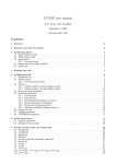
The essence of the quasi-static approximation is illustrated by Figure 1. When we calculate the plasma response,
the beam is considered as a rigid (not evolving in time) distribution of charges and currents which propagates
with the speed of light c. The fields generated by this beam depend on the longitudinal coordinate z and time
t only in combination ξ = z − ct and can be found layer-by-layer starting from the beam head. Since the beam
is not changing, all particles started from some transverse position r0 copy the motion of each other, and their
parameters (transverse coordinate and momenta) can be found as functions of ξ. Thus, a plasma macroparticle
in the quasi-static model is not a “big” particle, but a particle tube, i.e., a group of real particles started from
a given radius with a given initial momentum. This greatly reduces the memory required for storing plasma
particles.
simulation window
perfectly conducting walls
beam
(a)
unperturbed plasma before the beam
(b)
Figure 1: Geometry of the problem (a), and trajectory of a plasma particle in the simulation window (b).
The calculated fields are then used to modify the beam. For highly relativistic beams, the time step ∆t for
beam particles can be made large, which speeds up simulations several orders of magnitude. The quasi-static
approximation is thus useful if and only if the time scale of beam evolution is much longer than the period of
plasma wave.
Various details of LCODE and underlying physics are described in the following papers:
• K.V.Lotov, Simulation of ultrarelativistic beam dynamics in plasma wake-field accelerator. Phys. Plasmas
5 (1998), p.785-791. — The fluid plasma model.
• K.V.Lotov, Fine wakefield structure in the blowout regime of plasma wakefield accelerators. Phys. Rev.
ST - Accel. Beams 6 (2003), p.061301. — The beam model and the kinetic plasma model.
• K.V.Lotov, Blowout regimes of plasma wakefield acceleration. Phys. Rev. E 69 (2004), p.046405. —
Energy fluxes in the co-propagating window.
• K.V.Lotov, V.I.Maslov, I.N.Onishchenko, and E.N.Svistun, Resonant excitation of plasma wakefields by
a non-resonant train of short electron bunches. Plasma Phys. Control. Fusion 52 (2010), p.065009. —
Discussion on applicability of quasi-static codes to simulations of long beams.
• K.V. Lotov, A. Sosedkin, E.Mesyats, Simulation of Self-modulating Particle Beams in Plasma Wakefield
Accelerators. Proceedings of IPAC2013 (Shanghai, China), p.1238-1240. — Upgrade of the kinetic plasma
solver which was necessary for simulations of long beams.
2
Notation and units of measure
We use cylindrical coordinates (r, φ, ξ) for the axisymmetric geometry and Cartesian coordinates (x, y, ξ) for
the plane geometry. The beam propagates in positive ξ-direction.
The code works with dimensionless quantities. Units of measure depend on some basic plasma density n0 . It
is recommended to use the initial unperturbed plasma density as n0 . All times are in units of ωp−1 , where
2
√
ωp = 4πn0 e2 /m is the electron plasma frequency, e is the elementary charge, and m is the electron mass.
All distances are in units of c/ωp . The unit velocity is c. The notation used and units of measure for various
quantities are given in Table 1.
Table 1: Notation, units of measure, and places of first appearance
or definition for various quantities.
Notation
Quantity & place of definition
Unit
Times:
ωp−1
t
Time in general (Sec. 1) or propagation time for the beam
∆t
Main time step for the beam, Sec. 1, Sec. 5.1, time-step
′
∆t
Reduced time step for the beam, Sec. 5.1, beam-substepping-energy
tmax
Time limit for the run, Sec. 5.1, time-limit
tF
Period of the external beam focusing, Sec. 5.2, foc-period
tB
Oscillation period for the external magnetic field, Sec. 5.4, magnetic-field-period
∆tout
Periodicity of the detailed output, Sec. 5.6, output-period
Lengths:
c/ωp
ξ
The co-moving coordinate, Sec. 1
∆ξ
Longitudinal grid step, Sec. 3.1, Sec. 5.1, xi-step
⃗rb , rb , xb , ξb Coordinates of a beam macro-particle, Sec. 3.3
ξmax
Length of the simulation window, Sec. 5.1, window-length
∆r
Transverse grid step, Sec. 5.1, r-step
rmax
Transverse size of the simulation window, Sec. 5.1, window-width
rp , rp2
Width parameters for some plasma density profiles, Sec. 5.4.1, plasma-profile
Ltrap
Path limit for trapped plasma particles, Sec. 5.4.1, trapped-path-limit
ξsi
Check points for diagnosing beam survival (i = 1 . . . 6), Sec. 5.5, output-survival-xi
Xb0
Transverse displacement of the beam slice, Sec. 5.5, output-beam-slices
Rb , Xb
Radius or half-width of the beam slice, Sec. 5.5, output-beam-slices
ϵ
Emittance of the beam slice, Sec. 5.5, output-beam-slices
ξfrom , ξto
Left and right boundaries of the subwindow, Sec. 5.6.1, subwindow-xi-from
rfrom , rto
Bottom and top boundaries of the subwindow, Sec. 5.6.1, subwindow-xi-from
rax , raux
Two transverse coordinates to output functions of ξ at, Sec. 5.6.2, axis-radius
ls
Length of the beam segment, Sec. 6.1, length
δξ
Distance to beginning of the beam segment, Sec. 6.1, xishape
ξs
ξ-coordinate the segment begins at (ξs < 0), Sec. 6.1, xishape
σr
Transverse size of the beam segment, Sec. 6.1, xishape
σz
Length parameter for the Gaussian beam segment, Sec. 6.1, xishape
x0
Transverse displacement of the segment, Sec. 6.1, vshift
Velocities:
c
⃗v
Velocity of a plasma macro-particle or of an electron fluid element, Sec. 3.1, Sec. 3.2
⃗vi
Velocity of i-th plasma macro-particle, Sec. 3.1
⃗vb
Velocity of a beam macro-particle, Sec. 3.3
Momenta:
mc
p⃗
Momentum of a plasma macro-particle or of an electron fluid element, Sec. 3.1, Sec. 3.2
p⃗b
Momentum of a beam particle (not of a heavy macro-particle), Sec. 3.3
∆p foc
Extra momentum gained by a beam particle due to external focusing, Sec. 5.2, focusing
p⃗e
Momentum of a plasma electron, Sec. 5.6.1, colormaps-full
p⃗i
Momentum of a plasma ion, Sec. 5.6.1, colormaps-full
pb,ref
Reference value for displaying beam momentum, Sec. 5.6.4, output-reference-energy
pb0
Basic longitudinal momentum of beam particles in the segment, Sec. 6.1, energy
pa
Auxiliary value of the longitudinal momentum for the beam segment, Sec. 6.1, espread
Angular momentum:
mc2 /ωp
Mb
Angular momentum of a beam particle, Sec. 7.1
Masses:
m
M
Mass of a plasma macro-particle, Sec. 3.1
mb
Mass of a beam particle, Sec. 3.3
Number densities:
n0
ne
Density of plasma electrons, Sec. 3.2, Sec. 5.6.1, colormaps-full
ni
Density of plasma ions, Sec. 3.2, Sec. 5.6.1, colormaps-full
3
n(r)
np2
Initial transverse profile of the plasma density, Sec. 5.4.1, plasma-profile
A parameter for some plasma density profiles, Sec. 5.4.1, plasma-profile
Charge densities:
en0
ρ
Charge density of the plasma, Sec. 3.1
ρb
Charge density of the beam, Sec. 3.1, Sec. 5.6.1, colormaps-full
Current densities:
ecn0
⃗j
Total current density of plasma particles, Sec. 3.1
⃗jb
Current density of the beam, Sec. 3.1
Charges:
e
q
Charge of a plasma macro-particle, Sec. 3.1
qb
Charge of a beam particle, Sec. 3.3
Currents:
mc3 /e
Ib0
Base beam current, Sec. 5.2, beam-current
Ib
Current of the beam slice, Sec. 6.1, xishape
Fields:
E0 ≡ mcωp /e
⃗
E
Electric field in the plasma, Sec. 3.1
⃗
B
Magnetic field in the plasma, Sec. 3.1
Ẽr , B̃r
Auxiliary fields used in the kinetic plasma solver, Sec. 3.1
B0
External longitudinal magnetic field, Sec. 3.1, Sec. 5.4, magnetic-field-type
Bz0
Variation amplitude for the external magnetic field, Sec. 5.4, magnetic-field
Eaz
Average longitudinal electric field acting on the beam slice, Sec. 5.6.2, f(xi)
Potential:
mc2 /e
Φ
Wakefield potential, Sec. 3.2
Energies:
mc2
Wkin
Kinetic energy of a plasma electron, Sec. 3.1
Wss
Substepping energy for the beam, Sec. 5.2, beam-substepping-energy
Energy flux densities:
n0 mc3
⃗
S
Total energy flux density, Sec. 3.4, Sec. 5.6.1, colormaps-full
⃗f
S
Collective energy flux density, Sec. 3.4, Sec. 5.6.1, colormaps-full
⃗
Se
Electromagnetic energy flux density, Sec. 3.4, Sec. 5.6.1, colormaps-full
Energy fluxes:
n0 mc5 /ωp2
Ψ
Total energy flux along the simulation window, Sec. 3.4, Sec. 5.6.2, f(xi)
Ψf
Collective energy flux along the simulation window, Sec. 3.4, Sec. 5.6.2, f(xi)
Ψe
Electromagnetic energy flux along the simulation window, Sec. 3.4, Sec. 5.6.2, f(xi)
Energy densities:
n0 mc2
W
Total energy density, Sec. 3.4, Sec. 5.6.1, colormaps-full
Wf
Collective energy density, Sec. 3.4, Sec. 5.6.1, colormaps-full
Linear energy densities:
n0 mc4 /ωp2
Wint
Linear density of the total energy, Sec. 3.4, Sec. 5.6.2, f(xi)
dWint
Difference between total and collective linear energy densities, Sec. 3.4, Sec. 5.6.2, f(xi)
Distribution functions:
f⊥
Sec. 6.1, rshape
ωp /(m2 c3 )
f4d
Sec. 6.1, rshape
ωp2 /(m2 c4 )
f∥
Sec. 6.1, eshape
1/(mc)
Focusing strength:
mωp2
Fs
Strength of the external beam focusing, Sec. 5.2, foc-strength
Dimensionless:
qi
Charge of i-th plasma macro-particle, Sec. 3.1
A
Normalization factor for calculation of plasma currents and charge densities, Sec. 3.1
⃗ez
Unit vector in z-direction, Sec. 3.2
N
Quantity used by the fluid solver instead of the electron density, Sec. 3.2
γ
Relativistic factor of a plasma particle or of a fluid element, Sec. 3.2
Nr
Number of grid steps in the transverse direction, Sec. 5.1, r-step
l
Number of twofold reductions of the time step for a low-energy beam particle, Sec. 5.2,
beam-substepping-energy
Nb
Number of beam macro-particles in the slice of current Ib0 , Sec. 5.2.1,
beam-particles-in-layer
Dss
Maximum sub-stepping depth allowed for the kinetic plasma model (0 . . . 4), Sec. 5.4.1,
4
Asub
db
ηdraw
Nmr
Nmξ
Nav,r
Nav,ξ
Xm , Ym
Db
hfig
Nbins
γmin
Cstep
Ncol
αb
α0
Ia
substepping-depth
Sensitivity of the substepping trigger, Sec. 5.4.1, substepping-sensivity
Fraction of beam particles to output, Sec. 5.5, write-beam-particles
Fraction of the simulation window to be drawn as the full window, Sec. 5.6.1,
Number of grid points to be merged transversely into a single pixel on colored maps,
Sec. 5.6.1, colormaps-merging-r
Number of grid points to be merged longitudinally into a single pixel on colored maps,
Sec. 5.6.1, colormaps-merging-z
Rate of data smoothing in transverse direction, Sec. 5.6.1, colormaps-smoothing-r
Rate of data smoothing in longitudinal direction, Sec. 5.6.1, colormaps-smoothing-r
Substitutes for axis dimensions, Sec. 5.6.2, Sec. 5.6.3
Fraction of beam macro-particles to be drawn, Sec. 5.6.3, draw-each
Height of various pictures in pixels, Sec. 5.6.3, beam-picture-height
Number of histogram bins, Sec. 5.6.4, histogram-bins
Minimum relativistic factor for the plasma particle to be drawn, Sec. 5.6.5,
trajectories-min-energy
Color step for visualization of particle energies, Sec. 5.6.5, trajectories-energy-step
Ordinal number of a color in the palette, Sec. 5.6.5, trajectories-energy-step
Angular spread of the beam slice, Sec. 6, angshape
Maximum angular spread in the segment, Sec. 6, angspread
Maximum current in the beam segment, Sec. 6.1, ampl
Throughout the manual, the following highlighting conventions are used:
(filename.ext) — names of various files (small typewriter font in parentheses);
command -opt — execution commands (typewriter font);
option — configuration option (boldface);
3
3.1
Underlying physics
Kinetic plasma model
The equations solved for the fields are Maxwell equations, which in the dimensionless variables take the form
⃗
⃗ = ⃗j + ⃗jb + ∂ E ,
rot B
∂t
⃗
⃗ = − ∂B ,
rot E
∂t
⃗ = ρ + ρb ,
div E
⃗ = 0.
div B
(1)
Under the quasi-static assumption
∂
∂
∂
=− =
,
∂z
∂t
∂ξ
(2)
equations (1) result in
1 ∂
∂Ez
rEr = ρ + ρb −
,
r ∂r
∂ξ
1 ∂
∂Ez
r(Er − Bφ ) = ρ − jz ,
= jr ,
r ∂r
∂r
1 ∂
∂Bz
rBr = −
,
r ∂r
∂ξ
∂Bz
= −jφ ,
Eφ = −Br .
∂r
(3)
(4)
Here we neglect the components jbr and jbφ of the beam current and put jbz = ρb , since beam particles are
assumed to move mostly in z-direction. To provide stability of the algorithm, we solve in finite differences,
instead of (3), the following equations:
∂(ρ + ρb ) ∂jr
∂ 1 ∂
rEr − Er =
−
− Ẽr ,
∂r r ∂r
∂r
∂ξ
∂ 1 ∂
∂jφ
rBr − Br =
− B̃r ,
∂r r ∂r
∂ξ
(5)
where Ẽr and B̃r are some predictions for fields Er and Br . These equations are obtained by differentiation
of (3) and substitution of (4) into the result. Subtraction of the fields (with or without the tildes) from both
sides of the equalities does not produce a big error if the predictions are close to final fields. The boundary
conditions for equations (4)–(5) are those of a perfectly conducting tube of the radius rmax :
∫ rmax
2
Er (0) = Br (0) = Bφ (0) = Ez (rmax ) = Br (rmax ) = 0,
2πrBz dr = πrmax
B0 ,
(6)
0
5
where B0 is an external longitudinal magnetic field, if any (the presence of this field does not change the axial
symmetry of the system).
Each plasma macro-particle is characterized by 7 quantities: transverse coordinate (r), three components of the
momentum (pr , pφ , and pz ), mass M , charge q, and ordinal number. Parameters of plasma macro-particles are
initialized ahead of the beam (at ξ = 0) and then advanced slice-by-slice according to equations
])
d⃗
p
d⃗
p dt
q (⃗ [
⃗ ,
=
=
E + ⃗v × B
dξ
dt dξ
vz − 1
dr
vr
=
,
dξ
vz − 1
⃗v = √
p⃗
M 2 + p2
.
(7)
If a particle hits the wall (at r = rmax ), it is returned to the simulation area to some near-wall location with
zero momentum. Plasma current and charge density are obtained by summation over plasma macro-particles
lying within a given radial interval:
⃗j = A
∑
i
qi⃗vi
,
1 − vz,i
ρ=A
∑
i
qi
,
1 − vz,i
(8)
where A is a normalization factor. The denominator in (8) appears since the contribution of a “particle tube”
to density and current depends on the macro-particle speed in the simulation window.
calculation of plasma response
simulation window
layer b layer a
trajectory of a plasma
known
Dx
particle in simulation
response
window
r
beam
beam propagation
x=z-ct
Figure 2: Calculation of plasma response in the quasi-static approximation.
The plasma response is calculated layer-by-layer towards the decreasing ξ (from right to left in Fig. 2). As far as
for calculation of fields we need ξ-derivatives of currents, the following predictor-corrector scheme is used. We
first move plasma particles from layer a to layer b by the fields of the layer a, then calculate currents in layer b,
then calculate all fields in layer b, then move plasma particles from layer a to layer b by average fields of layers a
and b, then again calculate currents and fields in layer b, then again move plasma particles from layer a to layer
b by the average fields. When the fields are calculated first time, the radial fields from the previous layer are
taken as Ẽr and B̃r . When the fields are calculated second time, the earlier found average radial fields are used
as Ẽr and B̃r . Also, special efforts are made to suppress a small-scale (of the grid step size) plasma density noise.
The algorithm allows easy shortening of the ξ-step in the regions of a fine field structure. The shortening is
made automatically if the plasma current density |jz | exceeds some threshold value.
In the plane geometry, instead of equations (4), (5) we solve
∂ 2 Ex
∂(ρ + ρb ) ∂jx
− Ex =
−
− Ẽx ,
∂x2
∂x
∂ξ
∂(Ex − By )
∂Ez
∂Bz
= ρ − jz ,
= jx ,
= −jy ,
∂x
∂x
∂x
∂ 2 Bx
∂jy
− Bx =
− B̃x ,
∂x2
∂ξ
∂(Ex − By )
Ey = −Bx ,
= jx .
∂ξ
(9)
(10)
The last equation is used only at x = 0.9 rmax to find the integration constant for By . The boundary conditions
in the plane case are
∫ rmax
Ez (0) = Bx (0) = Ez (rmax ) = Br (rmax ) = 0,
Bz dx = rmax B0 .
(11)
0
6
3.2
Fluid plasma model
In the fluid approximation, the plasma is characterized by the density ne and momentum p⃗ of the electron
component. Plasma ions are the immobile background of the density ni = 1. Motion of the electron fluid is
governed by the equation
[
]
∂⃗
p
⃗ − ⃗v × B
⃗ ,
+ (⃗v ∇)⃗
p = −E
(12)
∂t
which, together with (1) and
√
⃗j = −ne⃗v ,
ρ = 1 − ne ,
⃗v = p⃗/γ,
γ = 1 + p2 ,
(13)
forms the complete set of equations. This set has two constants of motion. The first one was derived by Khudik
and Lotov1 :
⃗ = rot p⃗ + ne B0 (⃗ez − ⃗v ),
B
(14)
where B0 is the unperturbed longitudinal magnetic field ahead of the beam. The second one is well known and
comes from conservation of the generalized momentum:
Φ = γ − pz ,
(15)
where Φ is the wakefield potential:
Ez = −
∂Φ
,
∂ξ
Er − Bφ = −
∂Φ
.
∂r
(16)
It is convenient to use the quantity N = ne (1 − vz ) instead of the electron density ne and explicitly use the
continuity equation which takes the form
∂N
1 ∂ rN pr
=
.
(17)
∂ξ
r ∂r Φ
The final set of solved equations is, in the order of solving,
∂Φ
= −Ez ,
∂ξ
∂pr
∂pz
N pφ B0
1 ∂ ∂Φ
=
+ Bφ +
,
N =1+
r
,
∂ξ
∂r
Φ
r ∂r ∂r
1 + p2r + p2φ − Φ2
∂ 1 ∂
N pφ
∂N
∂Ez
N pr
rpφ −
= −B0
,
pz =
,
=−
,
∂r r ∂r
Φ
∂r
2Φ
∂r
Φ
N pr B0
∂pφ
1 ∂
Br = −Eφ = −
−
,
Bz =
rpφ + B0 N,
Φ
∂ξ
r ∂r
N
∂jb
∂ N
pr ∂ rN pr
N pr Ez
N 2 pφ B0
∂ 1 ∂
rBφ − Bφ =
− pz
+
+
+
.
∂r r ∂r
Φ
∂r
∂r Φ
Φ r ∂r Φ
Φ2
Φ2
(18)
(19)
(20)
(21)
Equations (18) are: the first equation of (16); the φ-component of (14) combined with (15); and the first
equation of (4). Equations (19) are: the z-component of (14) differentiated with respect to r and combined with
the third equation of (4); the definition of Φ (15) with the relativistic factor taken from (13); and the second
equation of (4). Equations (20) are: the last equation of (4); the r-component of (14); and the z-component
of (14). To obtain equation (21), we differentiate the z-component of the first equation in (1) with respect
to r, use the expression (19) for ∂Ez /∂r, and exclude ξ-derivatives of N , Φ, and pr with the help of (17) and (18).
In equations (18)–(21), only two quantities (Φ and pr ) need to be advanced to the next layer in ξ, all the others
can be expressed in terms of Φ and pr within the layer. The initial conditions for (18)–(21) are Φ = 1 and
pr = 0. The necessary boundary conditions are
∂(rBφ ) pφ (0) = pφ (rmax ) = 0,
Bφ (0) = Ez (rmax ) = 0,
= 0.
(22)
∂r r=rmax
Equations (18)–(21) are solved with the predictor-corrector scheme.
1 V.N.Khudik and K.V.Lotov, Ion channels produced by ultrarelativistic electron beams in a magnetized plasma. Plasma Physics
Reports, v.25 (1999), N 2, p.149-159.
7
In the plane geometry, the solved equations are
∂Φ
∂px
∂pz
N py B0
∂2Φ
∂ 2 py
N py
∂N
= −Ez ,
=
+ By +
,
N =1+
,
−
= −B0
,
2
∂ξ
∂ξ
∂x
Φ
∂x
∂x2
Φ
∂x
1 + p2x + p2y − Φ2
∂Ez
N px
N px B0
∂py
∂py
pz =
,
=−
,
Bx = −Ey = −
−
,
Bz =
+ B0 N,
2Φ
∂x
Φ
Φ
∂ξ
∂x
∂ 2 By
N
∂jb
∂ N
px ∂ N px
N px Ez
N 2 p y B0
− By =
− pz
+
+
+
,
2
2
∂x
Φ
∂x
∂x Φ
Φ ∂x Φ
Φ
Φ2
∂By ∂By py (0) = py (rmax ) = 0,
Ez (0) = Ez (rmax ) = 0,
=
= 0.
∂x ∂x x=0
3.3
(23)
(24)
(25)
(26)
x=rmax
Beam model
The beam is modeled by macro-particles. Each beam macro-particle is characterized by its longitudinal position ξb , transverse position rb or xb , three components of momentum p⃗b , charge qb , and mass mb . Equations of
motion for the macro-particles are
dξb
= vbz − 1,
dt
drb
= vbr ,
dt
[
]
d⃗
pb
⃗ + qb ⃗vb × B
⃗ ,
= qb E
dt
p⃗b
.
⃗vb = √ 2
mb + p2b
(27)
These equations are solved with the modified Euler’s method (midpoint method). The fields acting on the
macro-particle are linearly interpolated to the predicted macro-particle location at the half time step. If a
particle has a small longitudinal momentum and thus a high frequency of betatron oscillations, then the time
step for this particle is automatically reduced.
With no external magnetic field (B0 = 0), the angular momentum of beam particles must conserve, so the
azimuthal component of the momentum pbφ is not changed according to (27), but reconstructed from the
condition rb pbφ = const.
3.4
Energy fluxes and energy densities
In the presence of beams, there appears energy flows in the co-moving window2 . These flows are composed by
the energy flow in the laboratory frame and the energy transfer due to motion of the window. We can write the
perturbation to the dimensionless flux density of the electromagnetic energy
[
]
2
2
2
⃗e = −⃗ez E + B − B0 + E
⃗ ×B
⃗ ,
S
2
(28)
and the total energy flux density in the co-moving window
∑
⃗=S
⃗e +
S
(γ − 1)(⃗v − ⃗ez ),
(29)
where the summation is carried out over plasma particles in the unit volume. For the fluid plasma model, the
energy flux density is
⃗f = S
⃗e + ne (γ − 1)(⃗v − ⃗ez ).
S
(30)
⃗−S
⃗f , is the measure of the energy carried in the form of a thermal motion of
The difference of the two, S
plasma particles.
Integrating (28)–(30) across the simulation window gives us the energy fluxes against the z-axis:
r∫max
Ψe = −
Sez 2πr dr,
r∫max
Ψ=−
0
Sz 2πr dr,
0
r∫max
Ψf = −
Sf z 2πr dr.
(31)
0
It is easy to check that the total energy flux is the measure of beam-plasma energy exchange:
∂Ψ
=
∂ξ
r∫max
jbz Ez 2πr dr.
0
2 K.V.Lotov,
Blowout regimes of plasma wakefield acceleration. Phys. Rev. E, v.69 (2004), N 4, p.046405.
8
(32)
Thus, the drive beam puts energy to some point of the simulation window, and then this energy flows backward
or transversely until it exits the window or gets taken by a witness beam.
The difference between Ψ and Ψf can serve as a measure of the lost energy which cannot be retrieved by the
accelerated beam. In the absence of beams and nearby walls, the derivative ∂Ψ/∂ξ must be zero; this can be
used as a good test of precision for simulations.
The total energy density and fluid energy density are defined in the straightforward way:
W =
E 2 + B 2 − B02 ∑
+
(γ − 1),
2
Wf =
E 2 + B 2 − B02
+ ne (γ − 1),
2
(33)
correspondingly; summation is over plasma particles the unit volume.
4
Running the code
To run LCODE, execute the file (lcode.exe) (Windows) or (lcode) (UNIX, execute with ./lcode) in the
folder where the necessary input files are located. Possible (optional) input files are:
(lcode.cfg): the default configuration file (Sec. 5);
(beamfile.bin): the beam state file (Sec. 7.1);
(beamfile.bit): the continuation run indicator (Sec. 7.2);
(plasma.bin): the plasma state file (Sec. 7.3);
(fields.bin): the fields state file (Sec. 7.4);
arbitrarily named: other configuration files (Sec. 6), the beam constructor file (see beam-profile).
Additional command-line options can be provided after the executable name:
• Options --option=value overwrite options used in the main configuration file lcode.cfg.
• Directives filename.ext include other files containing configuration options.
• Special options interrupt the normal process of parsing command-line parameters and terminate execution
of the program with the following actions:
--help or --usage outputs a brief description of all possible configuration options.
--dump or --dump-config outputs the already read values of configuration options to console. To save
the output to a file (config.cfg), execute lcode.exe --dump-config > config.cfg (Windows) or
./lcode --dump-config > config.cfg (UNIX).
--dump-defconfig outputs the the configuration file with default values of options to console. To save
it to a file (default.cfg), execute lcode.exe --dump-defconfig > default.cfg (Windows) or
./lcode --dump-defconfig > default.cfg (UNIX).
--dump-docconfig outputs the the configuration file with default values of options, but in a more
detailed format. To save it to a file (docconfig.cfg), execute lcode.exe --dump-docconfig >
docconfig.cfg (Windows) or ./lcode --dump-docconfig > docconfig.cfg (UNIX).
If an option occurs several times in configuration files or command line, then the later value is used. The order
of reading the values is the following:
1. Initially, all options have the default hard-coded values (the ones specified as default in this manual,
Sec. 5).
2. The main configuration file ’lcode.cfg’, if present, with all the files included. The file is read from the
beginning to the end, with the included files, if any.
3. The command-line options processed left-to-right, if provided, with the included files if any.
Here are some examples of using command-line options:
./lcode
Executes LCODE with the values read from lcode.cfg, if present. (UNIX)
9
lcode.exe filename.cfg --beam-tune-charge=y
The same as above, but also reads values from (filename.cfg) and explicitly defines the beam-tunecharge option. (Windows)
lcode.exe filename1.cfg filename2.cfg --dump
First reads values from (lcode.cfg), if available; then reads values from (filename1.cfg) and
(filename2.cfg); then prints the resulting set of values to the screen. Simulations are not started. (Windows)
If the program is running in the terminal mode, its execution can be controlled by pressing some keys at the
terminal:
’,’ (comma): pause the execution before the next time step, can be used repeatedly to pause after each
time step;
’.’ (dot): stop the execution after finishing the time step, the run can be resumed afterwards;
’ ’ (space): pause the execution immediately;
’esc’ (escape): terminate the execution immediately;
’*’ (any key): resume the paused execution.
The
0
1
2
3
exit codes are:
— execution ends successfully;
— execution fails, the program prints an error message and terminates;
— the program was stopped manually with the dot key;
— the program was interrupted manually with the escape key.
The option values are validated after reading. If some values are invalid, then the program attempts an
automatic ’config recovery’ which consists of resetting the invalid values to the hardcoded defaults. This action
is indicated by warning messages. An example of a config recovery session is:
invalid histogram-bins=0 (Must be positive and <= 300) was reset to default 300
config recovered
Error filling config: invalid config, some defaults used
The config is still valid though
Trying to use a recovered config
If the recovery has been completed successfully, the program attempts execution with the recovered config.
The final (possibly recovered) configuration values at the start of computations are written to (lcode.runas.cfg)
to ease the diagnostics (see save-config, save-config-filename).
5
Configuration file
The configuration file is a text file containing the list of options in the form
option=value
or
option = value.
The order of options is of no importance. If an option is specifies several times, the later value is used.
Several options may coexist on the same line of the file, if they are separated by semicolons. Semicolons may
be omitted in several cases, but it is strongly recommended not to rely on that. The configuration file can
contain comments or empty lines which are ignored by the program, but improve visual readability of the file.
Comments begin with # and extend to the end of line.
In this section, configuration options are described like this:
option, type (default value): brief description
Detailed description, if necessary.
Possible types of options are:
choice: a value from a predefined set.
float: a floating-point number, may be in scientific notation.
string: a string (multiple characters). Strings with spaces, semicolons or hash signs must be enclosed in
double quotes, multiline strings must be enclosed in triple double quotes.
multichoice: multiple values from the predefined set, separated with commas.
10
y/n: ‘yes’ or ‘no’. Brief forms ‘y’ and ‘n’ are also possible.
The following is the list of options grouped by purpose. The options present in (lcode.runas.cfg), but not
described here, are under development.
5.1
Simulation area
geometry, choice (c): The geometry of the problem:
‘c’ or ‘axisymmetric’: Axisymmetric (cylindrical) geometry
‘p’ or ‘plane’: Plane (2d Cartesian) geometry
window-width, float (5): Transverse size of the simulation window, rmax
The radius in the cylindrical geometry or the full width in the plane geometry.
window-length, float (15): Length of the simulation window, ξmax
r-step, float (0.05): Transverse grid step, ∆r
The number of grid steps in the transverse direction, Nr , must not be too large: Nr = rmax /∆r ≤ 10000.
Otherwise ∆r is automatically increased.
xi-step, float (0.05): Longitudinal grid step, ∆ξ
time-limit, float (200.5): Time limit for the run, tmax
To insure against round off accumulation, put here a somewhat greater value than the last time moment
you wish to calculate.
time-step, float (25): Main time step for the beam, ∆t
continuation, choice (n): Mode of plasma continuation (Fig. 3):
‘n’ or ‘no’: Evolution of the beam. Every time step the beam enters an unperturbed plasma of a
prescribed profile.
‘y’ or ‘beam’: Evolution of the beam sequence. Every time step (except the first one) the beam
enters the perturbed plasma; the plasma state is taken from the end of the previous simulation
window. Does not work for the fluid plasma model.
‘Y’ or ‘longplasma’: Evolution of the plasma. A long beam creates the wake, and long-term behavior
of this wake is followed by the sequence of simulation windows. In this mode, only a rigid beam
can extend to several simulation windows. Does not work for the fluid plasma model.
Latter two regimes need ∆t = ξmax , otherwise ∆t is automatically corrected.
t
'Y'
'n'
simulation
windows
'y'
Dt
x=z-ct
xmax
Figure 3: Illustration of continuation modes.
5.2
Particle beams
beam-current, float (0.1): Base beam current (in 17 kA), Ib0
The common multiplier (in units of mc3 /e ≈ 17 kA) for dimensionless beam currents specified in
beam-profile. In the plane geometry corresponds to the current through c/ωp in the third dimension.
Also the unit current for beam macro-particles.
rigid-beam, y/n (n): Switch for evolution of the beam
‘y’ or ‘yes’: A rigid (not evolving in time) distribution of the beam current.
‘n’ or ‘no’: The beam is modeled by macro-particles.
11
beam-substepping-energy, float (2): Substepping energy for the beam, Wss
The threshold of reducing the time step for beam particles. For each beam particle, the minimal integer
l is found that meets the condition 22l (1 + pbz ) > Wss , and the reduced time step ∆t′ = ∆t/2l is then
determined. Plasma fields are calculated with periodicity ∆t, and each beam particle is propagating in
these fields with its own time step ∆t′ . This feature is particularly useful if low energy beam particles are
present in the system, which otherwise would require undesirable reduction of the main time step ∆t.
focusing, choice (n): External focusing for the beam:
‘n’ or ‘no’: No focusing
‘c’ or ‘cosine’: Cosine-varying focusing force. Each beam particle (located at radius rb ) at each time
step gets the extra radial momentum ∆p foc = Fs rb ∆t cos(2πt/tF ).
‘r’ or ‘rectangular’: Piecewise-constant focusing force. Each beam particle (located at radius rb ) at
each time step gets the extra radial momentum ∆p foc = ±Fs rb ∆t, where “+” is chosen if the
fractional part of (t/tF + 0.25) is less than 0.5, and “−” is chosen otherwise.
In the plane geometry, ∆p foc is the addition to x-momentum, and the distance between the particle and the midplane of the simulation window is used instead of rb .
foc-period, float (100): Period of the external focusing, tF
foc-strength, float (0.01): Strength of the external focusing, Fs
5.2.1
Newly generated beams
The following beam options determine parameters of newly generated particle beams or rigid beams. If the
beam is allowed to evolve by rigid-beam and the files (beamfile.bit) and (beamfile.bin) are present in the
working folder, then the beam state is imported from (beamfile.bin), the time is read from (beamfile.bit),
and these options are ignored.
beam-particles-in-layer, integer (200): Number of beam particles in the layer (≤ 100000), Nb
A beam slice which has the current Ib0 and length ∆ξ contains Nb macro-particles. Beam slices with lower
currents have correspondingly fewer macro-particles.
beam-profile, string (”xishape=cos, length=1”): Initial distribution of beam particles
The name of the file that specifies the initial distribution of beam particles in 6d phase space, or the initial
beam distribution itself (as a multiline description enclosed in triple quotes). If the value consists of a
single line without spaces or equal signs, it is interpreted as a filename to read the beam distribution from;
otherwise the value itself is considered the beam distribution description. The format of beam distribution
is described in Sec. 6.
beam-tune-charge, y/n (n): Tuning the charge of beam particles to match the beam profile better
‘n’ or ‘no’: All beam particles are equally charged. Only the absolute value of the charge can be
different. Consequently, the beam current can have only discrete values and therefore slightly
differs from the specified value.
‘y’ or ‘yes’: The charge of particles in each beam slice is slightly modified to better match the
specified beam profile. This option lowers the shot noise produced by the beam.
rng-seed, integer (1): Random generator seed
An integer number initiating the generator of random numbers. Different seeds generate different statistical
ensembles for the beam.
5.3
Laser beams
laser, choice (n): Enable laser beams
Option is under construction.
12
5.4
Plasma
plasma-model, choice (P): Plasma model:
‘f’ or ‘fluid’: The fluid model. It is the fastest one, but works only for the initially uniform plasma
with immobile ions. Neither wave-breaking, nor near-wall plasma perturbations are allowed.
‘p’ or ‘particles’: Obsolete kinetic model.
‘P’ or ‘newparticles’: New kinetic model described in Sec. 3.1.
magnetic-field, float (0): Variation amplitude for the external longitudinal magnetic field, Bz0
For zero Bz0 , the code runs faster since some equations (which are identically zeros) are not solved.
magnetic-field-type, choice (c): Time dependence of the external magnetic field seen by the beam:
‘c’ or ‘constant’: Always B0 = Bz0 .
‘r’ or ‘random’: B0 is a random value between 0 and Bz0 for each time step.
‘p’ or ‘periodic’: B0 = Bz0 cos(2πt/tB ).
magnetic-field-period, float (200): Period of magnetic field oscillations, tB
Used only with the periodic external magnetic field.
5.4.1
Options specific to particle plasma models
These options have effect only if plasma-model is a kinetic one.
plasma-particles-number, int (1000): Number of plasma macro-particles (≤ 40000)
All plasma electrons are modeled by this number of macro-particles. Mobile ions, if chosen, are modeled
by the same number of heavier macro-particles; in this case this number must be ≤ 20000.
plasma-profile, choice (1): The initial transverse profile of the plasma density (Fig. 4):
‘1’ or ‘uniform’: Uniform (= 1) up to the walls.
‘2’ or ‘stepwise’: Uniform (= 1) up to rp , zero at r > rp .
‘3’ or ‘gaussian’: Gaussian n(r) = exp(−r2 /2rp2 ), zero at r > 6rp ; obtained by variation of macroparticles weights.
‘4’ or ‘arbitrary’: Arbitrary, with particle parameters imported from (plasma.bin) and initial fields
from (fields.bin).
‘5’ or ‘channel’: Zero up to rp , uniform (= 1) at r > rp .
‘6’ or ‘sub-channel’: Constant (np2 ) up to rp2 , then linear growth from np2 to 1 between rp2 and rp ,
then 1 at r > rp ; obtained by variation of macro-particles weights.
For the plane geometry, the distance to the midplane |x − rmax /2| is used instead of r.
plasma-width, float (2): Main parameter of initial plasma density distributions, rp
plasma-width-2, float (1): Auxiliary parameter of initial plasma density distributions, rp2
plasma-density-2, float (0.5): Auxiliary parameter of initial plasma density distributions, np2
rp2 rp
'1'
1
1
'1'
'4'
n(r)
n(r)
'4'
np2 '6'
'5'
0 rp2 rp
(a)
'6'
np2
'3'
'2'
r
0
rmax
(b)
'5'
rmax /2
'3'
'2'
x
rmax
Figure 4: Illustration of possible plasma profiles in axisymmetric (a) and plane (b) geometries.
plasma-temperature, float (0): Initial temperature of mobile plasma particles in units of mc2
13
ion-model, choice (y): Model of plasma ions:
‘Y’ or ‘mobile’: Half of plasma macro-particles are single-charged mobile ions initially located at the
same positions as plasma electrons.
‘y’ or ‘background’: Ions are immobile background charge.
‘n’ or ‘absent’: No ions, plasma electrons are initially at rest.
ion-mass, float (1836): Ion mass in units of the electron mass (for mobile ions)
substepping-depth, integer (3): Maximum sub-stepping depth allowed (0 . . . 4), Dss
Substepping is usually needed for strongly nonlinear wakefields when some plasma particles are close to
trapping. If necessary, the longitudinal grid step can be automatically reduced up to 10Dss times with
respect to the basic xi-step.
substepping-sensivity, float (0.2): Sensitivity of substepping trigger, Asub .
If the longitudinal current density (jz ) is so high that the product of |jz | and ξ-step exceeds Asub at some
point, then the ξ-step is automatically divided by 10 (if allowed by substepping-depth). Reverse action
(increasing the ξ-step) is taken when jz gets small again.
trapped-path-limit, float (0): Path limit for trapped plasma particles, Ltrap
With this option, it is possible to treat trapping of plasma particles by the wakefield (to the extent allowed
by the quasi-static approximation). The charge of a macro-particle is put to zero when the time spent by
this macro-particle in the simulation window exceeds Ltrap . With this trick we obtain the correct plasma
state and fields at the distance Ltrap from the beam entrance to the plasma even if some plasma particles
get trapped by the wakefield. It is necessary to put Ltrap ≫ ξmax , otherwise the result will have no physical
meaning. Zero value of Ltrap switches this option off.
For every “trapped” macro-particle, 10 values are appended to file (captured.pls) (one particle per line):
1. Time
2. Number of the macro-particle (which contains information on its initial position)
3. Final ξ-coordinate
4. Final transverse coordinate
5-7. Final r-, φ-, and z-components of the particle momentum
8. Mass of the macro-particle
9. Charge-to-mass ratio
10. Relativistic factor
5.4.2
Option specific to the fluid plasma model
viscosity, float (0): Artificial viscosity
Artificial viscosity is used for suppressing high-frequency numerical noises or forcing the fluid model to
work beyond the applicability area. Reasonable values are between 0 and 0.01.
5.5
Every-time-step diagnostics
If activated, these diagnostics work at each main time step ∆t.
indication-line-format, choice (1): Format of the on-screen progress indication:
‘1’ or ‘eachdt’: One line each time step: time, total number of survived beam macro-particles,
maximum and minimum electric field Ez on the axis.
‘2’ or ‘eachdxi’: One line each ξ-step: time, |ξ|, Ez on axis, total energy flux Ψ, number of beam
macro-particles in this layer, number of sub-steps in ξ within the last ξ-step.
Location of the axis is determined by axis-radius. After finishing a time step (just before drawing pictures), the word “finished” is printed.
output-Ez-minmax, y/n (n): Write absolute extrema of the on-axis Ez into
output-Phi-minmax, y/n (n): Write absolute extrema of the on-axis Φ into
output-Ez-local, y/n (n): Write local extrema of the on-axis Ez into
14
(emaxf.dat)
(gmaxf.dat)
(elocf.dat)
output-Phi-local, y/n (n): Write local extrema of the on-axis Φ into
(glocf.dat)
If enabled, a line of 5 values is appended to the corresponding file immediately after an extremum is found:
1. Current time t
2. The maximum value of the quantity
3. ξ-coordinate of this maximum
4. The minimum value of the quantity (earlier found in case of local extrema)
5. ξ-coordinate of this minimum
Locations of the potential extrema are calculated more precisely than those of the field extrema. The
latter are found as multiples of the grid step ∆ξ.
output-beam-survival, y/n (n): Output of the number of survived beam particles
output-survival-xi, string (-2, -4, -6, -8, -10, -12): Check points for diagnosing beam survival
6 negative values separated by commas, in the descending order, ξsi (i = 1 . . . 6).
If enabled, then a line of 7 values is appended to file (n1.dat) at each time step:
1. Time t,
2-7. Number of survived beam macro-particles with ξb > ξsi
The information is written by one value immediately after passing ξsi .
output-beam-slices, y/n (n): Output of beam characteristics at selected cross-sections
output-slices-xi, string (-2, -4, -6, -8, -10, -12): Cross-sections for diagnosing beam properties
6 negative values separated by commas, in the descending order.
If the diagnostics is enabled, characteristics of 6 beam slices are appended to files (tt*.dat), where (*) is
a cross-section number (1 . . . 6). When the slice is passed, 6 values are appended to the corresponding file:
1. Time t,
2. On-axis electric field Ez at this ξ,
3. Emittance ϵ of the slice,
4. Beam transverse displacement Xb0 (is nonzero only in the plane geometry),
5. Beam radius Rb or half-width Xb ,
6. Number of beam macro-particles in this layer.
write-beam-particles, y/n (n): Output of individual characteristics of beam particles
If the diagnostics is enabled, then the following information about selected beam particles is appended to
file (partic.swp) at every time step, one line (9 values) per particle:
1. Time t,
2. Longitudinal coordinate ξb ,
3. Transverse coordinate rb or xb ,
4. Longitudinal momentum pbz ,
5. Transverse momentum pbr or pbx ,
6. Angular momentum Mb or third component of the momentum pby ,
7. Charge-to-mass ratio (absolute value),
8. Current carried by the particle,
9. Ordinal number.
The same particle characteristics can be also extracted from (beamfile.bin).
write-beam-particles-each, integer (1000): Fraction of beam particles to output, db
A beam particle is selected for output if its ordinal number is a multiple of db .
write-beam-particles-from, float (0): Right limit.
write-beam-particles-to, float (-10): Left limit
Only beam particles located between these two non-positive values are selected for output.
write-beam-particles-q-m-from, float (0): Lower limit for filtering beam particles by their q/m ratio
write-beam-particles-q-m-to, float (0): Upper limit for filtering beam particles by their q/m ratio
The interval of charge-to-mass ratios in which particles are written to (partic.swp). Equal values of these
parameters disable filtering.
output-lost-particles, y/n (n): Output of lost particles to (beamlost.dat)
If enabled, then beam particles which exit the simulation window are kept in file (beamlost.dat). One
line of 9 values is written for each particle. These values correspond to the last time particle was in the
simulation window. The file format is the same as for (partic.swp).
15
5.6
Periodical diagnostics
These diagnostics are periodically triggered with the time interval given by
output-period, float (100): Time periodicity of detailed output, ∆tout
If ∆tout < ∆t, then each time step is diagnosed. The first time step is always diagnosed.
5.6.1
Colored maps
These keys control output of various quantities as functions of r and ξ, either in the form of a colored map, or
in the form of a data array.
The colored maps are produced as separate files named (??*****[w].png) where (??) stands for two-character
quantity abbreviation, (*****) is the time of output, and the optional suffix ‘w’ denotes subwindow output.
Data arrays have the same naming abbreviations, but different extension: (??*****[m|w].swp). Suffix ‘m’
stands for full-window output, suffix ‘w’ denotes subwindow output. In the data files, one row is for one ξ-layer
or sub-layer. Columns correspond to different transverse coordinates.
colormaps-full, multichoice (””): A list of quantities to output in the full window
colormaps-subwindow, multichoice (””): A list of quantities to output in the subwindow
Full window means the drawn-portion of the whole simulation window, the area of size ξmax × rmax ηdraw .
Subwindow size and location are controlled manually. Output of the following quantities is possible:
.png
‘Er’: first transverse component of the electric field, Er or Ex
(er*****[w] .swp
)
.png
‘Ef’: second transverse component of the electric field, Eφ or Ey
(ef*****[w] .swp )
‘Ez’: z-component of the electric field, Ez
(ez*****[w] .png
)
.swp
‘Phi’: wakefield potential, Φ
(fi*****[w] .png
)
.swp
)
‘Bf’: φ or y component of the magnetic field, Bφ or By
(bf*****[w] .png
.swp
‘Bz’: perturbation of the longitudinal magnetic field, Bz − B0
(bz*****[w] .png
)
.swp
‘pr’: first transverse component of the electron momentum, per or pex
(pr*****[w] .png
)
.swp
‘pf’: second transverse component of the electron momentum, peφ or pey
(pf*****[w] .png
)
.swp
‘pz’: z-component of the electron momentum, pez
(pz*****[w] .png
)
.swp
‘pri’: first transverse component of the ion momentum, pir or pix
(ir*****[w] .png
)
.swp
‘pfi’: second transverse component of the ion momentum, piφ or piy
(if*****[w] .png
)
.swp
‘pzi’: z-component of the ion momentum, piz
(iz*****[w] .png
)
.swp
‘nb’: charge density of particle beams, ρb
(nb*****[w] .png
)
.swp
‘ne’: perturbation of the plasma electron density, ne − 1
(ne*****[w] .png
)
.swp
‘ni’: perturbation of the plasma ion density, ni − 1
(ni*****[w] .png
)
.swp
‘Sf’: z-component of the total energy flux density (e.f.d.), Sz
(sf*****[w] .png
)
.swp
‘Sr’: r-component of the total e.f.d., Sr
(sr*****[w] .png
)
.swp
‘dS’: z-component of the thermal e.f.d., Sz − Sf z
(sd*****[w] .png
)
.swp
‘Sf2’: r-weighted z-component of the total e.f.d., 2πrSz
(2f*****[w] .png
)
.swp
‘Sr2’: r-weighted r-component of the total e.f.d., 2πrSr
(2r*****[w] .png
)
.swp
‘dS2’: r-weighted z-component of the thermal e.f.d., 2πr(Sz − Sf z )
(2d*****[w] .png
)
.swp
‘Wf’: total energy density, W
(wf*****[w] .png
)
.swp
‘dW’: thermal energy density, W − Wf
(wd*****[w] .png
)
.swp
‘SEB’: z-component of the electromagnetic e.f.d., Sez
(se*****[w] .png
)
.swp
If a quantity is undefined (like electron momentum at points of zero electron density), then zero is output
at this point.
colormaps-type, choice (y): Controls whether functions of (r, ξ) are output as data files or as pictures:
‘n’ or ‘numbers’: Only data files.
‘y’ or ‘pictures’: Only pictures.
‘F’ or ‘both’: Both pictures and data files.
drawn-portion, float (1): Fraction of the simulation window to be referred as the full window, ηdraw
A number between 0 and 1 (Fig. 5a). Used to exclude uninteresting near-wall regions from the output.
subwindow-xi-from, float (-5): Right boundary of the subwindow, ξfrom
subwindow-xi-to, float (-10): Left boundary of the subwindow, ξto
subwindow-r-from, float (0): Bottom boundary of the subwindow, rfrom
subwindow-r-to, float (3): Top boundary of the subwindow, rto
Four parameters controlling the size and position of the subwindow (Fig. 5b).
16
axisymmetric:
hdraw rmax
hdraw rmax
Dr Nmr
pixels
plane:
rmax (1+h )
draw
2
xmax /Dx/Nmx pixels
r
0
x
-xmax
rmax (1-h )
draw
0 2
x
(a)
r to
(xfrom- xto)/Dx pixels
value
before
(rto -rfrom)/Dr
pixels
rfrom
xto
(b)
xfrom
after
cells
(c)
Figure 5: Physical and pixel sizes of the full-window colored map (a) and subwindow colored map (b); elementary
smoothing procedure (c).
colormaps-merging-r, integer (1): Merging in r, grid points, Nmr
colormaps-merging-z, integer (1): Merging in ξ, grid points, Nmξ
These numbers control output of one average value from several grid points (Fig. 5a). Values from the
specified number of grid points (Nmr in r and Nmξ in ξ) are added together and divided by the number
of points (Nmr Nmξ ). This procedure is made after the passage of the whole simulation window, when all
the values are written to an auxiliary file. The subwindow output is not affected by these options.
colormaps-smoothing-r, integer (0): Averaging in r, times, Nav,r
colormaps-smoothing-z, integer (0): Averaging in z, times, Nav,ξ
Smoothing out data arrays prepared for drawning as color maps. The elementary smoothing procedure
consists in delivering 1/4 of the value per adjacent cell (Fig. 5c). The procedure is repeated Nav,r times in
r-direction and Nav,ξ times in ξ-direction. Smoothing is made after merging of grid points, if any.
palette, choice (d): Colormap palette: default/greyscale/hue/bluewhitered
Coloring method used to display values of functions on (r, ξ) plane (Fig. 6):
‘d’ or ‘default’: Distinctly-colored palette
‘g’ or ‘greyscale’: Greyscale palette
‘h’ or ‘hue’: Hue-equidistant palette
‘b’ or ‘bluewhitered’: Blue-white-red palette
Each palette has 8 distinct colors for positive values of quantities and 7 colors for negative values. One
color is reserved for regions of zero density at plasma density maps (black for ‘default’ and ‘greyscale’
palettes, pure magenta for ‘hue’, and pure blue for ‘bluewhitered’).
The following parameters (color steps) set up a correspondence between the increment of a quantity and color
change on the picture:
E-step, float (0.1): Components of the electric field (‘Er’, ‘Ef’, ‘Ez’).
Phi-step, float (0.1): Wakefield potential (‘Phi’).
Bf-step, float (0.1): Transverse magnetic field (‘Bf’).
Bz-step, float (0.1): Longitudinal magnetic field (‘Bz’).
electron-momenta-step, float (0.1): Electron momenta (‘pr’, ‘pf’, ‘pz’).
ion-momenta-step, float (0.1): Ion momenta (‘pri’, ‘pfi’, ‘pzi’).
nb-step, float (0.1): Charge density of particle beams ( ‘nb’).
ne-step, float (0.1): Density of plasma electrons (‘ne’).
17
default
greyscale
hue
bluewhitered
Figure 6: Examples of colormap palettes.
Figure 7: Physical and pixel sizes of the figures showing functions of ξ and colors used for displaying output
quantities in the first group (top) and second group (bottom). The exact appearance of colors in the manual
may depend on the viewing software.
ni-step, float (0.01): Density of plasma ions (‘ni’).
flux-step, float (0.01): Components of energy flux densities ( ‘Sf’, ‘Sr’, ‘dS’, ‘SEB’).
r-corrected-flux-step, float (0.01): r-corrected energy flux densities (‘Sf2’, ‘Sr2’, ‘dS2’).
energy-step, float (0.01): Energy densities (‘Wf’, ‘dW’).
18
5.6.2
Functions of ξ
These keys control output of various quantities as functions of ξ, either in the form of a graph, or in the form
of a data array. The graphs are plotted in files named (u*****.png) or (v*****.png) by different colors, where
(*****) is the time of output (Fig. 7). Data arrays are named (u*****.swp) and (v*****.swp). Each line in the
data array correspond to certain ξ and contains 13 (u*****.swp) or 17 (v*****.swp) columns. First columns
in the files are values of ξ, others are output quantities. If a quantity is not chosen for output, zero value is
written in its place.
f(xi), multichoice (Ez,nb2,Ez2,dS,Sf,SEB): A list of quantities to output as functions of ξ.
The quantities can be listed in an arbitrary order.
There are two groups of quantities, which differ by files of output.
Indicated in braces are: the column number in the
data array (?*****.swp), the color of the graph in (?*****.png), the style of the graph.
First group:
(u*****. .png
)
.swp
‘ne’
{2, grey line}
ne (rax )
on-axis density of plasma electrons
‘nb’
{3, blue line}
ρb (rax )
on-axis charge density of the beam
‘Ez’
{4, green line}
Ez (rax )
on-axis z-component of the electric field
‘⟨Ez⟩’
{5, white line}
Eaz
average longitudinal electric field acting on the
beam slice
‘Bz’
{6, dark red line}
Bz (rax ) − B0
on-axis z-component of the magnetic field
‘Phi’
{7, yellow line}
Φ(rax )
on-axis wakefield potential
‘pz’
{8, dark green line}
pez (rax )
on-axis z-momentum of plasma electrons
‘emitt’ {9, green points}
ϵ
emittance of the beam slice
‘dW’
{10, dark grey line}
dWint
thermal energy per unit length
‘Wf’
{11, dark grey line}
Wint
total energy per unit length
‘ni’
{12, white line}
ni (rax )
on-axis density of plasma ions
‘pzi’
{13, dark green line} piz (rax )
on-axis z-momentum of plasma ions
.png
Second group:
(v*****. .swp
)
‘nb2’
{2, blue line}
ρb (raux )
off-axis charge density of the beam
‘Er’
{3, cyan line}
Er or Ex (raux )
off-axis transverse electric field
‘Ez2’
{4, green line}
Ez (raux )
off-axis longitudinal electric field
‘Bf’
{5, brown line}
Bφ or By (raux ) off-axis φ- or y component of the magnetic field
‘Bz2’
{6, dark red line}
Bz (raux ) − B0
off-axis z-component of the magnetic field
‘Fr’
{7, yellow line}
average focusing force, (Φaux − Φax )(raux − rax )
‘pr’
{8, dark blue line}
per or pex (raux ) off-axis r- or x-momentum of plasma electrons
‘pf’
{9, violet line}
peφ or pey (raux ) off-axis φ- or y-momentum of plasma electrons
{10, red points}
Rb or Xb
radius/width of the beam
‘⟨rb⟩’
{11, dark red points} 0 or Xb0
transverse displacement of the beam
‘dS’
{12, dark grey line}
Ψ − Ψf
integral thermal energy flux
‘Sf’
{13, dark grey line}
Ψ
integral total energy flux
‘SEB’
{14, dark grey line}
Ψe
integral electromagnetic energy flux
‘pri’
{15, dark blue line}
pir or pix (raux )
off-axis r- or x-momentum of plasma ions
‘pfi’
{16, violet line}
piφ or piy (raux ) off-axis φ- or y-momentum of plasma ions
‘Ef’
{17, magenta line}
Eφ or Ey (raux ) off-axis φ- or y component of the electric field
f(xi)-type, choice (n): Output mode for the functions of ξ:
‘y’ or ‘pictures’: Only pictures (u*****.png) and (v*****.png) are created.
‘Y’ or ‘numbers’: Only data files (u*****.swp) and (v*****.swp) are created.
‘F’ or ‘both’: Both pictures and data files are created.
‘n’ or ‘n’: No output of this kind.
axis-radius, float (0): Position of the ‘probe’ line 1, rax
auxiliary-radius, float (1): Position of the ‘probe’ line 2, raux
Two transverse positions at which functions of ξ are output. Both are measured from the geometrical axis
(in cylindrical geometry) or middle of the simulation window (in plane geometry). It makes sense to put
rax ̸= 0 only if the beam goes off-axis (in plane geometry) or if the plasma density is too noisy at the
geometrical axis (in cylindrical geometry).
The following parameters (Xm ) determine the size of the vertical axis when drawing functions of ξ (Fig. 7). The
axis is:
19
(0, Xm )
for fixed sign quantities,
(−Xm , Xm ) for sign-changing quantities.
For ion and electron densities, the axis type depends on Xm :
if Xm ≥ 1, then (0, Xm ),
the absolute value of the density is drawn,
if Xm < 1, then (−Xm , Xm ), the density perturbation is drawn.
E-scale, float (1): Most of the fields: ‘Er’,‘Ef’, ‘Ez’, ‘Ez2’, ‘⟨Ez⟩’, ‘Bf’, ‘Fr’
Phi-scale, float (1): Wakefield potential: ‘Phi’
Bz-scale, float (1): Longitudinal magnetic field: ‘Bz’, ‘Bz2’
electron-momenta-scale, float (1): Electron momenta: ‘pr, ‘pf’, ‘pz’
ion-momenta-scale, float (1): Ion momenta: ‘pri’, ‘pfi’, ‘pzi’
beam-radius-scale, float (5): Beam width and displacement: ‘⟨rb⟩’
nb-scale, float (1): Charge density of particle beams: ‘nb’, ‘nb2’
ne-scale, float (2): Density of plasma electrons: ‘ne’
ni-scale, float (1): Density of plasma ions: ‘ni’
flux-scale, float (1): Integral energy fluxes: ‘dS’, ‘Sf’, ‘SEB’
energy-scale, float (1): Energies per unit length: ‘dW’, ‘Wf’
emittance-scale, float (5): Beam emittance: ‘emitt’
5.6.3
Beam particle information as pictures
These keys control output of beam portraits in various parameter spaces. The selected beam macro-particles
are drawn as cyan dots in pictures (?*****.png), where (?) shows the content, and (*****) is the time.
output-beam-particles, multichoice (””): A list of beam projections to be drawn
Beam macro-particles can be output on the following planes in the following files:
‘r’: (r, ξ) plane (real space)
‘pr’: (pbr , ξ) plane (transverse momentum)
‘pz’: (pbz , ξ) plane (longitudinal phase space)
‘M’: (Mb , ξ) plane (angular momentum)
(p*****.png)
(r*****.png)
(z*****.png)
(m*****.png)
draw-each, integer (20): Fraction of beam macro-particles to be drawn, Db
A beam macro-particle is drawn if its ordinal number is a multiple of Db .
beam-picture-height, integer (300): Height of figures in pixels, hfig
This number determines the vertical size of f(xi) graphs, histograms, and beam portraits except the real
space portrait. The latter has the same height as colored maps (equal to ηdraw rmax /∆r/Nmr ).
output-reference-energy, float (1000): Reference value for displaying beam momentum, pb,ref .
The following parameters (Ym ) determine the size of the vertical axis for corresponding beam portraits:
beam-pr-scale, float (100): Axis is (−Ym , Ym ) for r-momentum of beam particles (‘pr’)
beam-a-m-scale, float (100): Axis is (0, Ym ) for the angular momentum of beam particles (‘M’)
beam-pz-scale, float (2000): Axis for z-momentum of beam particles (‘pz’)
The latter axis depends on the ratio between Ym and output-reference-energy pb,ref . If Ym > pb,ref , the
axis is (0, Ym ), otherwise it is (pb,ref − Ym , pb,ref + Ym ).
5.6.4
Beam information as histograms
These keys control output of beam characteristics in the histogram form, either as a picture (d?*****.png), or
as a data file (d?*****.swp), where (?) shows the content, and (*****) is the time. If a macro-particle falls
outside the chosen histogram interval, the particle is ignored.
Vertical size of the pictures in pixels is determined by beam-picture-height (Fig. 8a). The picture height in
physical units equals the highest column. To retain the normalization, the line of 3 values is appended to file
(hystog.dat) each time a histogram picture is produced. These values are:
1. Time
2. Histogram type (second character of the filename)
3. Height of the highest column.
The data files for histograms have 2 columns:
20
1. Number of the cell
2. Number of macro-particles in this cell.
Nbins pixels
hfig pixels
hdraw rmax
pixels
Dr Nmr
hdraw rmax units
xmax /Dx/Nmx pixels
-xmax
pb,ref
(a)
Ym
x
0
(b)
Figure 8: Exemplary histogram of beam longitudinal momentum (a) and trajectories of plasma particles in the
blowout regime (b).
histogram-output, multichoice (””): Output of various beam properties in the histogram form
Available options, corresponding output quantities, keys determining histogram intervals, and corresponding file names are:
‘r’: transverse momentum, pbr or pbx , beam-pr-scale,
(dr***** .png
)
.swp
‘z’: longitudinal momentum, pbz , beam-pz-scale,
(dz***** .png
)
.swp
‘M’: angular or y-momentum, Mb or pby , beam-a-m-scale,
(dm***** .png
)
.swp
‘a’: angle between the particle momentum and z-axis, beam-angle-scale,
(da***** .png
)
.swp
histogram-output-accel, multichoice (””): Output of histograms for accelerated particles only
The same as histogram output, but only beam macro-particles with z-momentum greater than outputreference-energy are taken into account. Available options, corresponding output quantities, keys determining histogram intervals, and corresponding file names are:
‘r’: transverse momentum, pbr or pbx , beam-pr-scale,
(dR***** .png
)
.swp
‘z’: longitudinal momentum, pbz , beam-pz-scale,
(dZ***** .png
)
.swp
‘M’: angular or y-momentum, Mb or pby , beam-a-m-scale,
(dM***** .png
)
.swp
‘a’: angle between the particle momentum and z-axis, beam-angle-scale,
(dA***** .png
)
.swp
histogram-type, choice (y): Mode of the histogram output:
‘y’ or ‘pictures’: Pictures only,
‘n’ or ‘data’: Data files only,
‘F’ or ‘both’: Both pictures and data files.
histogram-bins, integer (300): Number of histogram bins (≤ 3000), Nbins
beam-angle-scale, float (0.1): Axis size for the histogram of beam angular distribution
The axis is from zero to this value.
5.6.5
Trajectories of plasma particles
These diagnostics visualizes trajectories of plasma macro-particles in the simulation window, either as the
picture (pp*****.png) (Fig. 8b), or as the data file (*****.pls), where (*****) is the time. The diagnostics
works for kinetic plasma models only. Each line of the data file contains 9 values corresponding to one position
of one macro-particle:
1. Current ξ-coordinate
2. Number of the macro-particle
3. Transverse coordinate (r or x)
4-6. r-, φ-, and z-components of the particle momentum
21
7. Mass of the macro-particle
8. Charge-to-mass ratio
9. Relativistic factor
trajectories-draw, choice (n): Output mode for trajectories of plasma particles:
‘n’ or ‘n’: No output.
‘y’ or ‘y’: Picture mode. Trajectories of chosen plasma macro-particles on (r, ξ) plane are shown by
dotted lines with a specified interval in ξ between dots. The dot color represents the gammafactor γ of the particle. Sizes of the picture are the same as for full-window colored maps.
‘”Y”’ or ‘”Y”’: Data mode. Information about chosen macro-particles is written to the data file with
a specified interval in ξ between successive outputs.
‘F’ or ‘F’: Both picture and data file.
trajectories-each, integer (10): Fraction of plasma macro-particles to output
A trajectory of a plasma macro-particle can be drawn or written if the ordinal number of the macro-particle
is a multiple of this number.
trajectories-spacing, integer (10): Spacing in ξ for consecutive output of macro-particle parameters
This interval is measured in units of the grid step ∆ξ.
trajectories-min-energy, float (1): Minimum relativistic factor γ for the particle to be drawn, γmin
Particles with smaller relativistic factors are ignored. This is useful if you want to exclude weakly perturbed
plasma regions from the output.
trajectories-energy-step, float (0.5): Color step for visualization of particle energies, Cstep
The dot color in pictures is determined by Ncol = (γ − γmin )/Cstep . The order of colors is the same as for
the default palette of colored maps.
5.6.6
Detailed (substepped) plasma response
These keys control output of various plasma characteristics at a reduced ξ-step.
substepping-output-depth, integer (4): Substepping depth for the output (0..4)
How deep sub-stepping in ξ is included into the following output.
substepping-output-map, y/n (n): Substepped output of functions of (r, ξ)
If this option is enabled, then quantities chosen in colormaps-subwindow are also output with a reduced
ξ-step into data files named (??*****.det), where (??) is the two-character quantity abbreviation, and
(*****) is the time. The subwindow for the output is the same as for subwindow colored maps. No merging
or smoothing of values is made. If this diagnostics is on, the file (xi*****.det) is also created, which has
the same number of lines as data files and contains corresponding values of ξ, one value per line.
substepping-output-f(xi), y/n (n): Substepped output of functions of ξ
If enabled, then quantities chosen in f(xi) are also output with a reduced ξ-step into data files named
(u*****.det) and (v*****.det), where (*****) is the time. The file format is the same as for (u*****.swp)
or (v*****.swp).
substepping-output-particles, y/n (n): Substepped output of plasma particles
If enabled, information about plasma macro-particles is written to data file at each ξ-step or sub-step of the
depth specified by substepping-output-depth. Particle filtering criteria imposed by trajectories-each
and trajectories-min-energy are applicable.
substepping-output-particles-area, choice (f): Area for substepped output of plasma particles:
‘n’ or ‘no’: The output window is the same as for colored maps. Particle parameters are written to
file (*****.pls), where (*****) is the time.
‘y’ or ‘yes’: The output window is the same as subwindow for colored maps. Particle parameters
are written to file (s*****.pls), where (*****) is the time. The file format is the same as for
(*****.pls).
22
5.7
Saving run state
The following options control periodical savings of the run state.
saving-period, float (1000): Time interval between run saves
The run is saved if the time t differs from a multiple of the saving period by less then
made after completion of the ξ-cycle and drawing all pictures.
∆t/2.
Saving is
save-beam, y/n (n): Saving the beam state
The state of the beam is saved in binary file (tb*****.swp). The format of the file is the same as that of
(beamfile.bin). Option works for non-rigid beams only. Independently on this key, the beam state is also
saved to (beamfile.bin) on reaching the time limit tmax or after manual interruption of the run (by the
dot), so that the run can be continued without data loss.
save-plasma, y/n (n): Saving the plasma state
The plasma state at the end of the simulation window is saved to files (pl*****.swp) (plasma particles) and
(fl*****.swp) (electric and magnetic fields). Formats of the files are the same as those of (plasma.bin)
and (fields.bin) (Sec. 7.3, 7.4). Option works for kinetic plasma models only. Independently on this key,
in regimes with plasma continuation the final plasma state is saved to (plasma.bin) and (fields.bin) on
reaching the time limit tmax or after manual interruption of the run (by the dot), so that the run can be
continued without data loss.
The run can be resumed from any saved time ***** by changing the content of (beamfile.bit) to *****,
renaming (tb*****.swp) to (beamfile.bin), and, if necessary, renaming (pl*****.swp) to (plasma.bin) and
(fl*****.swp) to (fields.bin). Any changes in code options (e.g., changes of diagnostics) will take effect on
the resumed run.
5.8
Logging preferences
log-stdout-level, choice (d): Verbosity level for printing messages
log-file-level, choice (w): Verbosity level for logging to a file:
‘”e”’ or ‘”error”’: Output error messages only
‘”w”’ or ‘”warning”’: Output error and warning messages
‘”i”’ or ‘”info”’: Output error, warning and info messages
‘”d”’ or ‘”debug”’: Output error, warning, info and debug messages
log-filename, string (“lcode.log”): Name of the file to log to
log-file-clean, y/n (y): Remove empty log file
If enabled, then empty log files are automatically removed at the end of the run, if any.
save-config, y/n (y): Enable saving config to a file
save-config-filename, string (“lcode.runas.cfg”): Name of the file to save the current config to
This config includes the final version of all parameters, including those set by command-line switches. This
may become useful in later debugging, for exact replication of the execution process, and especially after
config recovery, as it reflects the automatic changes introduced by the recovery process.
6
Initial beam shape
There are two ways to define the initial distribution of beam particles in the six-dimensional phase space.
The first way is to specify all necessary parameters for each beam macro-particle. For this, information about
the macro-particles must be written to the binary file (beamfile.bin) by an external program. The initial time
must be written to the text file (beamfile.bit). The code will read this information as the initial state of the
beam.
The second way is to specify macroscopic parameters for individual beam segments. A segment is a beam piece
of variable length ls . The segments follow one by one starting from the beginning of the simulation window (at
ξ = 0). A description of a segment has the format
23
parameter1=value1, parameter2=value2, ..., parameterN=valueN
If a parameter definition not followed by comma, then it is considered as the last one in the description of this
segment. A description must contain at least one parameter defined. Segment descriptions follow one by one
in beam-profile or in a separate file which beam-profile refers to.
Numerical parameters can be specified in scientific notation (like 1e6) and postfixed with PI or Pi which acts
like multiplication by 3.1415926.
If a parameter is not explicitly defined in the segment description, then it is assigned the default value. The
initial default values are given in the following description. To modify default values for all subsequent segments,
a special line prefixed with ’default:’ can be used. This line has the same syntax as segment descriptions, but
does not define any segment and only changes the default values of some parameters. Re-definition of default
values can be made several times.
6.1
Segment parameters
length, float (2PI): Length of the segment, ls
ampl, float (0.5): Maximum current in the segment, Ia
Maximum current for this segment in units of beam-current Ib0 .
xishape, choice (c): Dependence of the beam current on the longitudinal coordinate, Ib (ξ)
In the following variants, the formulae are applicable in the interval ls > δξ > 0, where δξ = ξs − ξ, and
the segment starts at ξs ≤ 0.
‘c’ or ‘cos’: Shifted cosine shape,
Ib (ξ) = 0.5 Ia Ib0 (1 − cos(2πδξ/ls )).
‘t’ or ‘t’: Linear rise of the current,
Ib (ξ) = Ia Ib0 δξ/ls .
‘T’ or ‘T’: Linear decrease of the current,
Ib (ξ) = Ia Ib0 (1 − δξ/ls ).
‘l’ or ‘l’: Constant current,
Ib (ξ) = Ia Ib0 .
‘h’ or ‘half-cos’: Rising half-period of the shifted cosine,
Ib (ξ) = 0.5 Ia Ib0 (1 − cos(πδξ/ls )).
‘b’ or ‘b’: Decreasing half-period of the shifted cosine,
Ib (ξ) = 0.5 Ia Ib0 (1 + cos(πδξ/ls )).
‘g’ or ‘g’: Decreasing part of Gaussian function with σz = ls /6, Ib (ξ) = 0.5 Ia Ib0 exp(−18 δξ 2 /ls2 ).
radius, float (1): Radius of the beam segment, σr
energy, float (1000): Basic longitudinal momentum of beam particles, pb0
vshift, float (0): Transverse displacement of the segment (used in plane geometry only), x0
24
rshape, choice (g): Initial distribution of beam particles in the transverse phase space
Available options:
‘g’ or ‘gaussian’: Random distribution with the probability density
(
)
p2br + p2bφ
rb2
rb
f⊥ (rb , pbr , pbφ ) =
exp − 2 −
,
(axisymmetric beam),
2πσr2 αb2 p2b0
2σr
2αb2 p2b0
(
)
p2bx + p2by
1
(xb − x0 )2
f⊥ (xb , pbx , pby ) =
−
,
(plane geometry).
exp −
2σr2
2αb2 p2b0
(2π)3/2 σr αb2 p2b0
Here αb is the angular spread of the beam slice, and xb is measured from the central plane.
‘r’ or ‘regular’: The distribution with the same probability density as for ‘gaussian’, but with a
regular distribution of beam particles.
‘f’ or ‘flattop’:
Random distribution of particles with the “flattop” probability density in the
4-dimensional phase space,
(
)
(
)
p2by
1
(xb − x0 )2
p2bx
yb2
f4d (xb , yb , pbx , pby ) = 2 2 2 2 , if
+ 2 2
< 1 and
+ 2 2
< 1;
π σr αb pb0
σr2
αb pb0
σr2
αb pb0
f4d (xb , yb , pbx , pby ) = 0,
otherwise,
in which one spatial coordinate is ignored for each particle:
√
xb pbx + yb pby
yb pbx − xb pby
rb = x2b + yb2 , pbr =
, pbφ =
,
rb
rb
φb ignored, (axisymmetric),
yb ignored,
(plane).
angspread, float (1e-5): Maximum angular spread in the segment, α0
angshape, choice (l): Dependence of the angular spread on the longitudinal coordinate, αb (ξ)
In the following variants, the formulae are applicable in the interval ls > δξ > 0, where δξ = ξs − ξ, and
the segment starts at ξs < 0.
‘c’ or ‘cos’: Shifted cosine,
αb (ξ) = 0.5 α0 (1 − cos(2πδξ/ls )).
‘t’ or ‘t’: Linear rise,
αb (ξ) = α0 δξ/ls .
‘T’ or ‘T’: Linear decrease,
αb (ξ) = α0 (1 − δξ/ls ).
‘l’ or ‘l’: Constant,
αb (ξ) = α0 .
‘h’ or ‘half-cos’: Rising half-period of the shifted cosine, αb (ξ) = 0.5 α0 (1 − cos(πδξ/ls )).
‘b’ or ‘b’: Decreasing half-period of the shifted cosine,
αb (ξ) = 0.5 α0 (1 + cos(πδξ/ls )).
‘g’ or ‘g’: Decreasing part of Gaussian function,
αb (ξ) = 0.5 α0 exp(−18 δξ 2 /ls2 ).
espread, float (0): Auxiliary value of the longitudinal momentum, pa
eshape, choice (m): Longitudinal momentum distribution of beam particles, f∥ (pbz )
Available options:
‘m’ or ‘monoenergetic’: Monoenergetic,
f∥ (pbz ) = δ(pbz − pb0 ).
‘u’ or ‘uniform’: Uniform over the interval,
f∥ (pbz ) = (pb0 − pa )−1
if pb0 > pbz > pa ,
f∥ (pbz ) = 0 (
otherwise.
)
‘l’ or ‘linear’: Linear energy growth from pa to pb0 ,
f∥ (pbz ) = δ pbz − pb0 δξ/ls − pa (1 − δξ/ls ) .
2
2
e−(pbz −pb0 ) /(2pa )
√
‘g’ or ‘gaussian’: Gaussian distribution,
f∥ (pbz ) =
2πpa
‘N’ or ‘N’: N monoenergetic fractions (N is a digit, 2 . . . 9),
N
−1
∑
i
(pb0 − pa )
f∥ (pbz ) =
δ(pbz − pi ),
pi = pa +
N −1
i=0
m/q, float (1): Absolute value of mass-to-charge ratio, compared to the electron
25
6.2
Example of a beam profile
default: angspread=3e-3, energy=2000
xishape=cos, ampl=1, length=6PI
xishape=len, ampl=0, length=1e6
The first line redefines the default values for two options.
The second line defines the beam segment of the length 6π, current Ib (ξ) = 0.5 Ib0 (1 − cos(|ξ|/3)), and Gaussian
transverse distribution (hardcoded default value) with σr = 1 (hardcoded default value) and αb = 0.003
(hardcoded default ξ-dependence, new default value). All particle in the segment have the same longitudinal
momentum (hardcoded default distribution) that equals 2000 (new default value). Particles are either electrons
or positrons, depending on the sign of Ib0 .
The second line defines the space extending from ξ = −6π to ξ = −1000000 − 6π with zero current and thus
no particles.
7
7.1
Format of other input and output files
beamfile.bin
This file contains information about beam macro-particles in the binary form. For each particle, 8 values are
are written, 8 bytes each (type double). These values are:
1. Longitudinal position, ξb .
2. Transverse position, rb (cylindrical geometry) or xb (plane geometry).
3. Longitudinal momentum, pbz .
4. Transverse momentum, pbr (cylindrical geometry) or pbx (plane geometry).
5. Angular momentum Mb (cylindrical geometry) or third momentum component pby (plane geometry).
6. Absolute value of the charge-to-mass ratio, compared to electron.
7. Charge carried by the macro-particle. The charge unit is ∆ξmc2 /(2e).
8. Ordinal number of the macro-particle.
As follows from the data format, the actual beam density depends on the longitudinal grid step xi-step. If
the beam generated with some ∆ξ is used in a continuation run with different ∆ξ, then the beam density seen
by the code will differ from the original one by the ratio of grid steps. The reason is that different number of
macro-particles add together to form the total beam current in each particular grid layer.
The last macro-particle in (beamfile.bin) always has ξb = −100000.0 and serves as the end-of-file sign.
7.2
beamfile.bit
Contains the current time (a decimal number in the text form) and serves as the indicator of the continuation
mode. If this file is present, the code tries to continue a previous run.
7.3
plasma.bin
File (plasma.bin) contains information about plasma macro-particles (one line for one macro-particle). It has
6 columns:
1. Transverse coordinate of the macro-particle (r or x) counted from the bottom of the simulation window.
2. First component of the transverse momentum (pr or px ) of the macro-particle (not of a single electron
or ion). It equals the particle velocity times relativistic factor times “mass” of the macro-particle.
3. Second component of the transverse momentum (pφ or py ) of the macro-particle.
4. Longitudinal momentum (pz ) of the macro-particle.
5. “Mass” of the macro-particle. For uniform electrons of the unit density (i.e., of the density n0 ), the
“mass” is just the cross-section corresponding to this macro-particle (it is a ring in the cylindrical geometry or
a rectangle in the plane geometry). For heavier particles, the “mass” is correspondingly greater.
6. “Charge” of the macro-particle. It is the “mass” times the real charge-to-mass ratio for particles of
this sort.
When the run is normally terminated or interrupted in the regimes of a long plasma, the final parameters of
all macro-particles are automatically saved to (plasma.bin). If the run is then continued, the initial plasma
26
parameters are taken from (plasma.bin). The same happens if a new run is started with an arbitrary initial
plasma profile.
7.4
fields.bin
File (fields.bin) contains information about the fields and plasma currents. Each line in (fields.bin)
corresponds to a grid point. Number of lines is Nr + 1 (number of grid steps plus one). Each line contains
8 values:
Er , Eφ , Ez , Bφ , Bz , pr , pφ , pz for cylindrical geometry and fluid plasma model,
Ex , Ey , Ez , By , Bz , px , py , pz for plane geometry and fluid plasma model,
Er , Eφ , Ez , Bφ , Bz , jr , jφ , jz for cylindrical geometry and kinetic plasma model,
Ex , Ey , Ez , By , Bz , jx , jy , jz for plane geometry and kinetic plasma model.
Here pα are components of the electron momentum; jα are components of the total current density.
When the run is normally terminated or interrupted in the regimes of a long plasma, the final fields are
automatically saved to (fields.bin). For kinetic plasma models, the run can be then continued with the initial
fields taken from (plasma.bin). The same happens if a new run is started with an arbitrary initial plasma profile.
7.5
r*****.det
This file contains auxiliary information for subwindow diagnostics (Sec. 5.6.1, 5.6.6). If any sub-window diagnostics is on, then 3 values are written (not appended) to file (f*****.det), where (*****) is the time:
1. Transverse grid step.
2. Lower boundary of the sub-window.
3. Number of ξ-steps inside the sub-window.
7.6
Diagnostics files
These files are generated by diagnostic tools described in corresponding sections of the manual, and their format
is explained on the following pages:
File name
Section Page
File name
Section Page
(beamlost.dat) 5.5
15
(captured.pls) 5.5
14
(elocf.dat)
5.5
15
(s*****.pls)
5.6.6
21
(emaxf.dat)
5.5
15
(*****.pls)
5.6.5
21
(glocf.dat)
5.5
15
(??*****m.swp) 5.6.1
16
(gmaxf.dat)
5.5
15
(??*****w.swp) 5.6.1
16
(hystog.dat)
5.6.4
20
(d?*****.swp)
5.6.4
20
(n1.dat)
5.5
15
(fl*****.swp)
5.7
27
(tt*.dat)
5.5
15
(partic.swp)
5.5
15
(??*****.det)
5.6.6
16
(pl*****.swp)
5.7
26
(u*****.det)
5.6.6
19
(tb*****.swp)
5.7
26
(v*****.det)
5.6.6
19
(u*****.swp)
5.6.2
19
(xi*****.det)
5.6.6
22
(v*****.swp)
5.6.2
19
7.7
Temporary files
Files (aver.swp), (digcol.swp), (digcol2.swp), (bfile.swp), (info.swp), (??*****.swp) are temporary files and
are always deleted in normal regimes
27