Download NMAG User Manual (Incomplete DRAFT)

NMAG User Manual (Incomplete DRAFT)
Author:
Author:
Author:
Author:
Author:
Author:
Licence:
Version:
SVN-Version:
This document:
Hans Fangohr
Thomas Fischbacher
Matteo Franchin
Giuliano Bordignon
Michael Walter
Jacek Generowicz
GNU General Public License (GPL)
manual.txt 4253 2007-10-04 12:03:44Z fangohr
4249:4253
compiled 2007-10-04 at 12:58.
Outline of document
1 Introduction
1.1 Nmag Philosophy
1.2 How to read this document
2 Guided Tour
2.1 Example: Demag field in uniformly magnetised sphere
2.1.1 Importing nmag
2.1.2 Creating the simulation object
2.1.3 Defining (magnetic) materials
2.1.4 Loading the mesh
2.1.5 Setting the initial magnetisation
2.1.6 Setting the external field
2.1.7 Extracting and saving data
2.1.7.1 Saving averaged data
2.1.7.2 Extracting arbitrary data from the running programme
2.1.7.3 Saving spatially resolved data
2.2 Example 2: Computing the time development of a system
2.2.1 Mesh generation
2.2.2 The simulation
2.2.3 Analysing the data
2.2.3.1 Time dependent averages
2.2.3.2 Spatially resolved fields
2.2.4 ... these are the basics
2.2.5 “Relaxing” the system
2.2.6 “Relaxing” the system faster
2.3 Example: Hysteresis loop for Stoner-Wohlfarth particle
2.3.1 Hysteresis simulation script
1
2.3.2 Hysteresis loop computation
2.3.3 Obtaining the hysteresis loop data
2.3.4 Plotting the hysteresis loop with Gnuplot
2.4 Example: Hysteresis loop for thin disk
2.4.1 Thin disk hysteresis loop
2.5 Example: Vortex formation and propagation in disk
2.6 Example: Manipulating magnetisation
2.6.1 Modifying the magnetisation
2.7 Example: IPython
2.8 Example: Pinning Magnetisation
2.8.1 Pinning simulation script
2.8.2 Pinning magnetisation
2.8.3 Visualisation
2.9 Example: Uniaxial anisotropy
2.9.1 Unixaial anisotropy simulation script
2.9.2 Visualization
2.9.3 Comparison
2.10 Example: Cubic Anisotropy
2.10.1 Cubit anisotropy simulation script
2.10.2 Analyzing the result
2.11 Example: Thermal Effects
2.11.1 Thermal effects simulation script
2.11.2 Simulating thermal effects
2.11.3 Comparison of runs at different temperatures
2.12 Example: Larmor precession
2.13 Example: 1D periodicity
2.14 Example: 2D periodicity
2.15 Restart example
2.16 Timestepper parameter example
2.17 Periodic boundary conditions
2.18 Parallel execution
3 Background
3.1 The nsim library
3.2 Fields and subfields
3.2.1 Field
3.2.2 Subfield
3.3 Fields and Subfields in Nmag
3.3.1 Example: one magnetic material
3.4 Mesh
3.4.1 Node
3.4.2 node id
3.4.3 node position
3.5 Site
3.6 SI object
2
3.7 Terms
3.7.1 Stage, Step, iteration, time
3.7.2 Some geek-talk deciphered
4 Command reference
4.1 MagMaterial
4.1.1 uniaxial_anisotropy
4.1.2 cubic_anisotropy
4.2 Simulation
4.2.1 advance_time
4.2.2 get_subfield
4.2.3 get_subfield_positions
4.2.4 get_subfield_sites
4.2.5 probe_subfield
4.2.6 probe_H_demag
4.2.7 hysteresis
4.2.8 load_mesh
4.2.9 relax
4.2.10 save_data
4.2.11 set_m
4.2.12 set_H_ext
4.2.13 set_pinning
4.3 SI
4.3.1
4.3.2
4.3.3
4.3.4
value
units
in_units_of
is_compatible_with
5 Finite element mesh generation
5.1 Nmesh file format
5.1.1 Ascii nmesh
5.1.2 Hdf5 nmesh
5.2 mesh file size
5.3 Conversion of mesh files into nmesh format
6 Executables
6.1 ncol
6.2 nmagpp
6.3 nsim
6.4 nmeshpp
6.4.1
6.4.2
6.4.3
6.4.4
General information (--info)
Inspecting the quality of a mesh
Histogram of edge lengths
nmeshimport
7 Files and file names
7.1 mesh file (.nmesh, .nmesh.h5)
7.2 Simulation scripts (.py)
3
7.3 Data files (.ndt)
7.4 Data files (.h5)
7.5 File names for data files
7.6 File names for log files
8 Frequently asked questions
8.1 What’s the difference between OOMMF and nmag?
8.2 Why do you have your own Python interpreter (=“nsim“)?
9 Useful tools
9.1 vtk
9.2 MayaVi
9.3 NumPy
10 Acknowledgements
1 Introduction
Nmag is a flexible, finite element based micromagnetic simulation package with an user interface based on the Python
programming language.
1.1 Nmag Philosophy
The majority of specialized simulation codes used in research today consists of a highly specialized core application
which was written initially to simulate the behaviour of some very specific system. Usually, the core application then
evolved into a more broadly applicable tool through the introduction of additional parameters. Some simulation codes
reach a point where it becomes evident that they need an amount of flexibility that can only be provided by including
some script programming capabilities.
The approach underlying Nmag turns this very common pattern of software evolution (which we also have seen in
web browsers, CAD software, word processors, etc) on its head: rather than gradually providing more and more
flexibility in an ad-hoc manner through adding configuration parameters, slowly evolving into an extensive specialized
programming language, Nmag starts out as an extension to a widely used programming language from which it gains
all its flexibility and evolves towards more specialized notions to conveniently define the properties of very specific
systems.
The main advantage of this approach is two-fold: first, we do not gradually evolve another ad-hoc (and potentially
badly implemented) special purpose programming language. Second, by drawing upon the capabilities of a well
supported existing framework for flexibility, we get a lot of additional power for free: the user can employ readily
available and well supported libraries for tasks such as data post-processing and analysis, e.g. generating images
for web pages etc. In addition to this, some users may benefit from the capability to use Nmag interactively from a
command prompt, which can be very helpful during the development phase of an involved simulation script.
The disadvantage is of course that a novice user may be confronted with much more freedom than he can handle.
We try to cope with this issue by providing a collection of example scripts for the most common applications that only
need very slight modification (e.g. changing of the mesh filename or material parameters) for basic use.
At present, Nmag is based on the Python programming language. This seems to be a somewhat reasonable choice
at present, as Python is especially friendly towards casual users who do not want to be forced to first become expert
programmers before they can produce any useful results. Furthermore, Python is quite widespread and widely
supported these days. As most of the underlying field theoretical foundations used by Nmag are derived from the
low level nsim multiphysics simulator which is not closely tied to Python, it would be possible to provide support for
other scripting languages in the future should the need arise (e.g. in case Python should become unpopular over the
years).
4
1.2 How to read this document
We suggest you follow the Guided Tour through a number of examples to get a quick overview of what nmag looks like
in real use, and to see examples that can be used to carry out typical simulations. We provide a number of skeletons
that are easily adapted to specific systems which show how to compute hysteresis loops, do energy minimisation, or
compute time evolution.
The Command Reference section explains the relevant commands provided by Nmag in full detail. This should be
especially useful to advanced users who want to design sophisticated simulation scripts in Python.
2 Guided Tour
We present a number of examples, together with more detailed explanation of their structure.
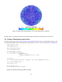
2.1 Example: Demag field in uniformly magnetised sphere
This example computes the demagnetisation field in a uniformly magnetised sphere. We know, of course, that the
demag field has to have the opposite direction to the magnetisation, and a magnitude of 1/3 of the magnetisation in
this special case.
When using finite element calculations, a crucial (and non-trivial) part of the work is the finite element mesh generation. We provide a very small mesh for this example (sphere1.nmesh.h5) which was generated with Netgen. It
describes a sphere of radius 10nm.
Using this, we can write the following nmag script with name sphere1.py:
import nmag
from nmag import SI
#create simulation object
sim = nmag.Simulation()
# define magnetic material
Py = nmag.MagMaterial(name = ’Py’,
Ms = SI(1e6, ’A/m’),
exchange_coupling = SI(13.0e-12, ’J/m’)
)
# load mesh
sim.load_mesh(’sphere1.nmesh.h5’,
[(’sphere’, Py)],
unit_length = SI(1e-9, ’m’))
# set initial magnetisation
sim.set_m([1,0,0])
# set external field
sim.set_H_ext([0,0,0], SI(’A/m’))
# Save and display data in a variety of ways
sim.save_data(fields=’all’) # save all fields spatially resolved
# together with average data
# sample demag field through sphere
for i in range(-10,11):
x = i*1e-9
#position in metres
H_demag = sim.probe_subfield_f(’H_demag’, [x,0,0])
print "x =", x, ": H_demag = ", H_demag
5
To execute this script, we have to give its name to the nsim executable, for example (on linux):
user@host user> nsim sphere1.py
Let’s discuss the sphere1.py script step by step.
2.1.1 Importing nmag
First we need to import nmag, and any subpackages of nmag that we need (this is just the SI object).
import nmag
from nmag import SI
2.1.2 Creating the simulation object
Next, we need to create a simulation object.
sim = nmag.Simulation()
2.1.3 Defining (magnetic) materials
After having imported the nmag module into Python’s workspace and after creating the simulation object sim, we
need to define a material using nmag.MagMaterial. We give it a name (as a Python string) which in this case is "Py"
and we assign a saturaration magnetisation and an exchange coupling strength.
Py = nmag.MagMaterial(name = ’Py’,
Ms = SI(1e6, ’A/m’,
exchange_coupling = SI(13.0e-12, ’J/m’))
The name of the material chosen here plays an important role as all the Fields and Subfields will automatically be
given names which include this material name. The output files will also use that name to label output data.
All data input and output within nmag is expressed in SI units by default. To avoid ambiguity here but simultanouesly
provide flexibility in the choice of input and output units, an SI object is provided. This has to be used when defining
the material parameters (and in some other places). We thus express the saturation magnetisation in Ampere per
metre (Ms = SI(1e6,"A/m")) and the exchange coupling constant (often called A in micromagnetism) in Joules per
metre (exchange_coupling = SI(13.0e-12, "J/m")).
2.1.4 Loading the mesh
The next step is to load the mesh.
sim.load_mesh(’sphere1.nmesh.h5’,
[(’sphere’, Py)],
unit_length = SI(1e-9, ’m’))
The first argument is the file name ("sphere1.nmesh.h5"). The second argument is a list of tuples which describe
the domains (also called regions) within the mesh. In this example we have a list with one tuple: ("sphere", Py).
The first element of the tuple, "sphere", is a string (of the user’s choice) and this is the name given to mesh region 1
(i.e. the space occupied by all simplices that have the region id 1 in the mesh file).
[This information is currently only used for debugging purposes (such as when printing the simulation object).]
The second part of the tuple is the MagMaterial object that has been created in Defining (magnetic) materials and
bound to the variable Py. This object determines the material properties of the material in this domain; in this example,
we have specified the properties of PermAlloy.
The third argument to load_mesh is an SI object which defines what real distance should be associated with the
length 1.0 as given in the mesh file. In this example, the mesh has been created in nanometres, i.e. the distance 1.0
in the mesh file should correspond to 1 nanometre in the real world. We thus use an SI object of 1nm.
6
2.1.5 Setting the initial magnetisation
To set the initial magnetisation, we use the set_m method.
sim.set_m([1,0,0])
The field m describes the normalised magnetisation whereas the field M contains the magnetisation with its proper
magnitude (i.e. |M| is the saturation magnetisation, whereas |m|=1.0). For this simulation, we provide a unit vector
pointing in the x-direction to indicate that we would like the initial magnetisation to point in the positive x-direction. (We
could provide a vector with non-normalised magnitude, which would be normalised automatically. This is convenient
for, say, magnetisation pointing 45 degrees between x and y axis: [1,1,0]).
2.1.6 Setting the external field
We could set the external field using the set_H_ext command
sim.set_H_ext([0,0,0], SI(’A/m’))
In contrast to set_m, this method takes two arguments. The first defines numerical values for the direction and
magnitude of the external field. The second determines the meaning of these numerical values using an SI object. Suppose we would like an external field of 1e6 A/m acting in the y-direction, then the command would read:
sim.set_H_ext([0,1e6,0],SI(1,"A/m")). However, we could also use sim.set_H_ext([0,1,0],SI(1e6,"A/m")).
The default value for the external field is [0,0,0] A/m, so for this example, we could have ommitted the set_H_ext
command altogether.
2.1.7 Extracting and saving data
We have three different ways of extracting data from the simulation
1. saving averaged values of fields (which can be analysed later)
2. saving spatiallialy resolved fields (which can be analysed later)
3. extracting field values at arbitrary positions from within the running programme
In the sphere1 example discussed here, we use all three methods and will discuss these in more detail now:
2.1.7.1 Saving averaged data
sim.save_data()
The save_data method writes averages of all fields (see Fields and subfields) into a text file. This file is best analysed
using the ncol tool but can also just be read with a text editor. The format follows OOMMF’s odt fileformat: every row
corresponds to one snap shot of the system (see save_data).
The function can also be called with parameters to save spatially resolved field data (see Saving spatially resolved
data).
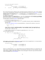
The first and second line in the file are headers that explain the entity and the units of the entity saved in the
corresponding column.
The ncol tool allows to extract particular columns easily so that these can be plotted later (useful for hysterises loop
studies). In this example where have only one “timestep”, there is only one row of data in this file and we shall not
explore this further here.
2.1.7.2 Extracting arbitrary data from the running programme
The line
H_demag = sim.get_subfield_f( ’H_demag’, [x,0,0] )
obtains the demagnetisation field (see Fields and subfields in nmag) at position (x,0,0). By default, the position is
specified in SI units, and the data returned are also expressed in SI units.
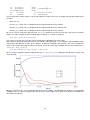
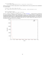
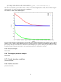
The for-loop in the programme (which iterates x in the range from -10*1e-9 to 10*1e-9 in steps of 1e-9) produces the
following output
7
x
x
x
x
x
x
x
x
x
x
x
x
x
x
x
x
x
x
x
x
x
=
=
=
=
=
=
=
=
=
=
=
=
=
=
=
=
=
=
=
=
=
-1e-08 : H_demag =
-9e-09 : H_demag =
-8e-09 : H_demag =
-7e-09 : H_demag =
-6e-09 : H_demag =
-5e-09 : H_demag =
-4e-09 : H_demag =
-3e-09 : H_demag =
-2e-09 : H_demag =
-1e-09 : H_demag =
0.0
: H_demag =
1e-09 : H_demag =
2e-09 : H_demag =
3e-09 : H_demag =
4e-09 : H_demag =
5e-09 : H_demag =
6e-09 : H_demag =
7e-09 : H_demag =
8e-09 : H_demag =
9e-09 : H_demag =
1e-08 : H_demag =
None
[-329655.76203912671, 130.62999726469423, 194.84338557811344]
[-329781.46587966662, 66.963624669268853, 137.47161381890737]
[-329838.57852402801, 181.46249265908259, 160.61298054099865]
[-329899.63327447395, 131.06488858715838, 71.383139326493094]
[-329967.79622912291, 82.209856975234786, -16.893046828024836]
[-329994.67306536058, 61.622521557150371, -34.433041910642359]
[-329997.62759666931, 23.222244635691535, -65.991127111463769]
[-330013.90370482224, 10.11035370824321, -61.358763616681067]
[-330023.50844056415, -6.9714476825652287, -54.900260456937708]
[-330030.98847923806, -26.808832466764223, -48.465748009067141]
[-330062.38479507214, -38.660812022013424, -42.83439139610747]
[-330093.78111090627, -50.512791577262625, -37.2030347831478]
[-330150.72580001026, -64.552170478617398, -23.120555702674721]
[-330226.19050178828, -77.236085707456397, -5.5373829923226916]
[-330304.59300913941, -90.584413821813229, 14.090609104026118]
[-330380.1392610991, -115.83746059068679, 37.072085708324757]
[-330418.85831447819, -122.47512022500726, 62.379121138009992]
[-330476.40747455234, -110.84257225592108, 108.06217226524763]
[-330500.20126762061, -68.175725285038382, 162.46166752217249]
[-330517.86675206106, -24.351273685146875, 214.40344001233677]
At position -1e-8, there is no field defined (this is just outside the mesh) and therefore the value None is returned.
We can see how the demagnetisation field varies slightly throughout the sphere. The x-component is approximately
a third of the magnetisation, and the y- and z-components are close to zero (as would be expected for a perfectly
round sphere).
We mention for completeness that most fields (such as magnetisation, exchange field, anisotropy field etc) are only
defined within the region occupied by the magnetisation. However, there is a special function to probe the demagnetisation field anywhere in space (XXX to be documented, Ticket:19).
2.1.7.3 Saving spatially resolved data
The command
sim.save_data(fields=’all’)
will save all fields (see Fields and subfields) spatially resolved for the current configuration into a file with name
sphere1_dat.h5. (It will also save the spatially average values as described in Saving averaged data.) Whenever the
save_data function is called, it will write the averaged field values into the ndt file.) This name is, by default, based
on the name of the simulation script, but can be overridden with an optional argument to the Simulation constructor.
The data in this file are in compressed binary format (build on the hdf5 standard) and can be extracted and converted
later using the nmagpp tool.
For example, we can dump the magnetisation field to stdout (which is typically the screen) using:
nmagpp --dump sphere1
However, here we are interested in creating a vtk file for visualisation purposes from the saved data. We use:
nmagpp --vtk sphere1.vtk sphere1
where sphere1.vtk is the name of the vtk file that is to be generated.
Once this is executed, we can visualise the data. For this manual we use MayaVi as the visualisation tool for vtk files
but there are others avialable (see vtk).
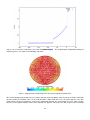
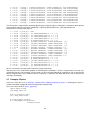
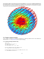
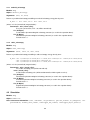
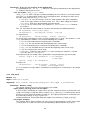
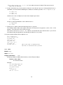
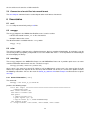
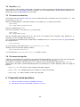
We start MayaVi and load the vtk data file with mayavi -d sphere1.vtk. Using MayaVi’s menus, we can add a
“VelocityVector” module to display the magnetisation:
8
The magnetisation is pointing in the x-direction (because we initialised the magnetisation in this orientation by issuing
the command sim.set_m([1,0,0])).
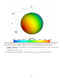
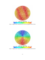
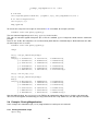
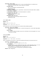
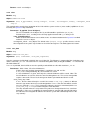
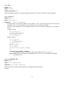
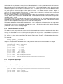
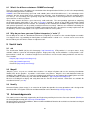
The demagnetisation field should point in the opposite direction of the magnetisation. Let’s first create a colour-coded
plot of the scalar magnetic potential, phi, from which the demag field is computed by taking the negative gradient:
9
We can see that the potential varies along the x-direction. The legend at the bottom of the figure shows the colour
code used. We can also see from the legend title that the units of the potential phi are Ampere (this is the <A>).
Unless the user specifies a particular request for the units of data, the following rules apply for vtk files:
• position are given in the same coordinates as the mesh coordinates (that is why the x, y and z axis have values
going from -10 to 10).
• all field data are given in SI units.
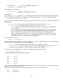
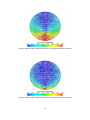
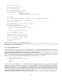
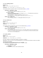
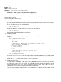
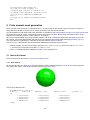
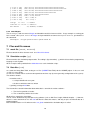
The next plot shows the demag field (the vectors) together with isosurfaces of the magnetic potential:
10
It can be seen that the isosurfaces are completely flat planes (i.e. the potential is changing only along x) and the
demagnetisation field is perpendicular to the isosurfaces. The colorbar on the left refers to the magnitude of the
demagnetisation field which is expressed in Ampere per metre as can be seen from the label <A/m>.
2.2 Example 2: Computing the time development of a system
This example computes the time development of the magnetisation in a bar with dimensions 30nm in the x and y
directions and 100nm in z-direction. The initial magnetisation is pointing in the [1,0,1] direction, i.e. 45 degrees away
from the x axis in the direction of the z-axis. We first show the simulation code and then discuss it in more detail.
2.2.1 Mesh generation
While it is down to the mesh generation software (see also Finite element mesh generation) to explain how to generate
finite element meshes, we briefly show the steps necessary to create a mesh for this example in Netgen, and how to
convert it into an nmesh mesh.
1. The finite element method requires the domain of interest to be broken down into small regions: the finite
elements. Such a subdivision of space is known as a mesh or grid. We use Netgen to create this mesh.
Netgen reads a geometry file which tells it what geometry to mesh. To create the mesh used here, start
Netgen and load the geometry file by using the menu: File-> Load Geometry. Then tell Netgen that we
like the edge length to be shorter than 3 by going to Mesh->Meshing Options->Mesh Size and enter 3.0
in the max mesh-size box. Then click on the Generate Mesh button to generate the mesh. Finally, using
File->Export save the mesh as a neutral file (this is the default) under the name bar30_30_100.neutral.
(We provide a gzipped version of this file for completeness here.)
2. This neutral file needs to be converted into a nmesh file. We do this using:
11
nmeshimport --netgen bar30_30_100.neutral bar30_30_100.nmesh.h5
By providing the .h5 extension, we write a compressed mesh file which is significantly smaller than an
ascii file (see mesh file size).
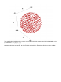
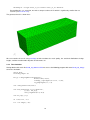
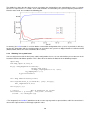
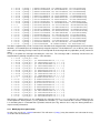
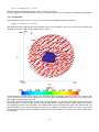
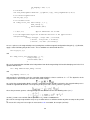
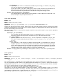
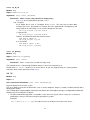
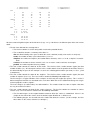
The generated mesh is shown here:
We can examine the mesh using nmeshpp to find out about the mesh quality, the statistical distribution of edge
lengths, and the overall number of points and elements etc.
2.2.2 The simulation
Having obtained the mesh file bar30_30_100.nmesh.h5 we can use the following program with name bar30_30_100.py
to run the simulation:
import nmag
from nmag import SI
mat_Py = nmag.MagMaterial(name="Py",
Ms=SI(0.86e6,"A/m"),
exchange_coupling=SI(13.0e-12, "J/m"),
llg_damping=SI(0.5,""))
sim = nmag.Simulation("bar")
sim.load_mesh("bar30_30_100.nmesh.h5",
[("Py", mat_Py)],
unit_length=SI(1e-9,"m"))
sim.set_m([1,0,1])
dt = SI(5e-12, "s")
for i in range(0, 61):
12
sim.advance_time(dt*i)
#compute time development
if i % 10 == 0:
#every 10 loop iterations,
sim.save_data(fields=’all’)
#save averages and all
#fields spatially resolved
else:
sim.save_data()
#otherwise just save averages
As in Example demag field in uniformly magnetised sphere, we import nmag and create the the material object.
import nmag
from nmag import SI
mat_Py = nmag.MagMaterial(name="Py",
Ms=SI(0.86e6,"A/m"),
exchange_coupling=SI(13.0e-12, "J/m"),
llg_damping=SI(0.5,""))
We set the llg_damping parameter to 0.5. To be consistent with the other input parameters for the material, this
needs to be an SI object without units - this is why we write SI(0.5,"").
The next line creates the simulation object.
sim = nmag.Simulation("bar")
Here, we provide a name for the simulation object, i.e. bar. This will be used as the root of the name of any data
files that are being written. If this name is not specified (as in Example demag field in uniformly magnetised sphere),
it defaults to the name of the file that contains the script (but without the .py extension).
Next, we load the mesh file, and set the initial (normalised) magnetisation to point in the [1,0,1] direction, i.e. to
have equal magnitude in the x- and z-direction and 0 in the y-direction.
sim.load_mesh("bar30_30_100.nmesh.h5",
[("Py", mat_Py)],
unit_length=SI(1e-9,"m"))
sim.set_m([1,0,1])
This vector will automatically be normalised within nmag, so that [1,0,1] is equivalent to the normalised vector
[0.70710678,0,0.70710678].
In this example, we would like to study a dynamic process and will ask nmag to compute the time development over
a certain amount of time dt. The line:
dt = SI(5e-12, "s")
simply creates an SI object which represents this amount of time (i.e. 5 pico seconds) over which to carry out that
integration.
We then have a Python for-loop in which i will take integer values ranging from 0 to 60 for subsequent iterations. All
indented lines are the body of the for-loop.
for i in range(0, 61):
sim.advance_time(dt*i)
if i % 10 == 0:
sim.save_data(fields=’all’)
else:
sim.save_data()
13
In each iteration, we first call sim.advance_time(i*dt) which instructs nmag to carry out the integration up to a time
i*dt.
The call to save_data will save the average data into the bar_dat.ndt file.
The last four lines contain an if statement and are used to save the data. The percent operator % computes i modulo
10. This will be 0 when i takes values 0, 10, 20, 30, ..., i.e. every 10 iterations. In this case, we call:
sim.save_data(fields=’all’)
which will save the (spatial) averages of all fields (going into the bar_dat.ndt file), and the spatially resolved data for
all fields (that are saved to bar_dat.h5).
If i is not an integer multiple of 10, then the command:
sim.save_data()
is called, which saves only the spatially averaged data.
2.2.3 Analysing the data
2.2.3.1 Time dependent averages
First, we will plot the average magnetisation vector against time. To see what data is available, we call ncol with just
the name of the simulation (which here is bar):
$> ncol bar
0:
#time
1:
id
2:
step
3:
stage_time
4:
stage_step
5:
stage
6:
E_total_Py
7:
phi
8:
E_ext_Py
9:
H_demag_0
10:
H_demag_1
11:
H_demag_2
12:
dmdt_Py_0
13:
dmdt_Py_1
14:
dmdt_Py_2
15:
H_anis_Py_0
16:
H_anis_Py_1
17:
H_anis_Py_2
18:
m_Py_0
19:
m_Py_1
20:
m_Py_2
21:
M_Py_0
22:
M_Py_1
23:
M_Py_2
24:
E_anis_Py
25:
E_exch_Py
26:
rho
27:
H_ext_0
28:
H_ext_1
29:
H_ext_2
30: H_total_Py_0
31: H_total_Py_1
32: H_total_Py_2
33:
E_demag_Py
34:
H_exch_Py_0
#<s>
<>
<>
<s>
<>
<>
<kg/ms^2>
<A>
<kg/ms^2>
<A/m>
<A/m>
<A/m>
<A/ms>
<A/ms>
<A/ms>
<A/m>
<A/m>
<A/m>
<>
<>
<>
<A/m>
<A/m>
<A/m>
<kg/ms^2>
<kg/ms^2>
<A/m^2>
<A/m>
<A/m>
<A/m>
<A/m>
<A/m>
<A/m>
<kg/ms^2>
<A/m>
0
1
0
0
0
0
-0.2603465789714
0.0002507410390772
0
-263661.6680783
-8.218106743355
-77027.641984
-8.250904652583e+15
2.333344983225e+16
8.250904652583e+15
0
0
0
0.7071067811865
0
0.7071067811865
608111.8318204
0
608111.8318204
0
5.046530179037e-17
0.03469702141876
0
0
0
-263661.6680783
-8.218106743352
-77027.641984
-0.2603465789714
3.301942533099e-11
14
35:
H_exch_Py_1
36:
H_exch_Py_2
37: maxangle_m_Py
38:
localtime
39:
unixtime
<A/m>
<A/m>
<deg>
<>
<s>
0
3.301942533099e-11
0
2007/08/15-11:16:19
1187172979.6
The meaning of the various entries is discussed in detail in section ncol. Here, we simply note that the number of the
left row is
• 0 for the time,
• 21 for M_Py_0 which is the x-component of the magnetisation of the Py material,
• 22 for M_Py_1 which is the y-component of the magnetisation of the Py material, and
• 23 for M_Py_2 which is the z-component of the magnetisation of the Py material,
We can use ncol to extract this data into a file data_M.dat which has the time for each time step in the first column
and the x, y and z component of the magnetisation in columns 2, 3 and 4, respectively:
ncol bar 0 21 22 23 > data_M.txt
This creates a text file data_M.txt that can be read by other applications to create a plot.
Note, however, that the order of the entries in the ndt file is not guaranteed, i.e. the numbers corresponding to fields
may change with different versions of the software, or different simulations (for example: the user may add extra
fields). The recommended way therefore is to directly specify the name of the columns that are to be extracted (i.e.
time M_Py_0 M_Py_1 M_Py_2):
ncol bar time M_Py_0 M_Py_1 M_Py_2 > data_M.txt
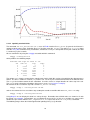
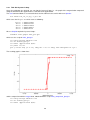
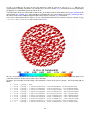
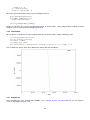
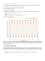
We use xmgrace to plot this data by calling it with xmgrace -nxy data_M.txt, adding the legend and axis labels, and
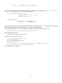
create this plot:
We have carried out the same simulation with Magpar and OOMMF. The following plot shows the corresponding
OOMMF-curves (as spheres) together with nmag’s results. (The magpar curve, which is not shown here, follows the
nmag data very closely.)
15
2.2.3.2 Spatially resolved fields
The command sim.save_data(fields=’all’) saves all Fields into the file bar_dat.h5 (in general, the filename is
composed of the name of the simulation [here bar] and the extension _dat.h5). The code bar30_30_100.py above
calls the save_data command every 10 iterations, and because every dt corresponds to 0.5 pico seconds, the data
is saved every 5 pico seconds.
We can confirm this by using the nmagpp executable with this command:
nmagpp --timesteplist bar
which produces the following output:
Available time steps for field ’m’ are
row
time <s>
step
stage
0
0
0
1
1
5e-11
307
1
2
1e-10
562
1
3
1.5e-10
1002
1
4
2e-10
1471
1
5
2.5e-10
1584
1
6
3e-10
1668
1
The column row is simply a counter for the stored entries for this field. We used to select which of the data to process
further. The time is shown in seconds (<s>) and we can see the 5 pico second interval between the different rows.
The step is the iteration counter for the calculation. It can be used as a unique identifier of a time step in the run.
The stage is only relevant for calculations of hysterises curves (see hysteresis example).
We convert the first saved time step into a vtk file bar_initial.vtk using
nmagpp --range 0 --vtk bar_initial.vtk bar
and we also convert the last saved time step at 300 pico seconds to avtk file with name bar_final.vtk using:
nmagpp --range 6 --vtk bar_final.vtk bar
Using MayaVi, we can display this data in a variety of ways. Remember that all field values are shown in SI units
by default (see nmagpp), and positions are as provided in the mesh file. In this case, positions are expressed in
nanometers (this comes from the unit_length=SI(1e-9,"m") expression in the sim.load_mesh() command.
The following image shows the initial magnetisation pointing in the [1,0,1] direction:
16
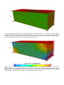
The final configuration show that the magnetisation aligns along the z-direction. The coloured surface show the
x-component of the magnetisation (and the colorbar provides the scale). It can be seen that the magnetisation at
position z=100 nm goes into a flower state to minimise the overall energy (note that stricly speaking this system is
not in a meta-stable state yet but a snap shot of a dynamical process):
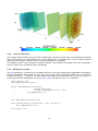
Because we have saved all fields (not just the magnetisation), we can also study other properties. For example, the
following image shows the demagnetisation field as vectors (and the legend refers to the magnitude of the vectors),
and the magnetic scalar potential is shown via 10 isosurfaces. Because the demagnetisation field is the (negative)
gradient of the scalar potential, the vectors are perpendicular on the isosurfaces:
17
2.2.4 ... these are the basics
The examples above provide an overview of the fundamental commands used to setup a micromagnetic calculation
and used to progress the configuration of the system through time. In principle, this is all one needs to know to
compute hysteresis loops and carry out the common micromagnetic calculations.
The following sections (and subsequent examples) introduce some higher-level functions that make computing a
hysterises loop easier, and provide further functionality.
2.2.5 “Relaxing” the system
The relax command is a function of the simulation that takes the current magnetisation configuration and computes
the time development until the torque on each mesh site is smaller than a certain threshhold. This is useful for the
example of our bar as -- in general -- we don’t know for how long we need to integrate the system until it stops in a
local energy minimum configuration. Here is the source code changed to use the relax command:
import nmag4 as nmag
from nmag4 import SI,every,at
mat_Py = nmag.MagMaterial( name="Py",
Ms=SI(0.86e6,"A/m"),
exchange_coupling=SI(13.0e-12, "J/m"),
llg_damping=SI(0.5,"")
)
sim = nmag.Simulation("bar_relax")
sim.load_mesh("bar30_30_100.nmesh.h5", [("Py", mat_Py)], \
unit_length=SI(1e-9,"m"))
sim.set_m([1,0,1])
18
s = SI(1,"s")
#get SI dimensions for seconds
sim.relax(save = [(’averages’, every(’time’,5e-12*s)),
(’fields’, at(’convergence’))])
We’ll explain the relax command:
sim.relax(save = [(’averages’, every(’time’,50e-12*s)),
(’fields’, at(’convergence’))])
in more detail.
The argument save = [ ] is telling the relax function that it should save data according to the following instructions.
There are two objects provided in the list between the square brackets ([ and ]). here. The first one is this tuple:
(’averages’, every(’time’,50e-12*s)
and means that the averages should be saved every 50 pico seconds. The syntax that is used breaks down in the
following parts:
• ’averages’ is just the keyword (a string) to say that the average data should be saved
• every(...) is a special object which takes two parameters. They are here:
– ’time’ to indicate that something should be done every time a certain amount of simulated time
has passed and
– 50e-12*s which is the amount of time after which the data should be saved again. This has to
be a SI object (and this is achieved in this example by multipyling a number (50e-12) with the SI
object s which just represents one second and has been defined in our example program.
– We can provide further keywords to the every object (for example to save the data every n iteration steps we can use every(10,’step’)). The relax command uses the hysteresis command
internally, so this can be used to look up more explanation.
The second object in the list is:
(’fields’, at(’convergence’))
and means that the fields should be saved at convergence, i.e. when the relaxation process has finished and the
magnetisation has converged to its (meta)stable configuration:
• ’fields’ is a string that indicates that we would like to save all the defined fields.
• at(’convergence’) is a special object that indicates that this should happen exactly when the relaxation process has converged, i.e. at the end of the simulation in this example.
After having run this programme, we can use the ncol tool to look at the averages saved:
ncol bar_relax step time
we get the following output (only the beginning shown):
0
82
120
146
176
201
227
248
0
5e-12
1e-11
1.5e-11
2e-11
2.5e-11
3e-11
3.5e-11
which shows the iterations on the left and the simulated time (in seconds) on the right. As requested, there is one
data entry (i.e. line) every 5 pico seconds.
Note that it may happen, that the system saves the data not exactly at the requested time, i.e.:
532
580
620
6.5e-11
7.047908066945e-11
7.5e-11
19
The middle line shows that the data has been saved when the simulated time was approximately 7.05e-11 seconds
whereas we requested 7e-11 seconds. Such small deviations are tolerated by the system to improve performance2.
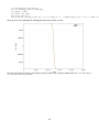
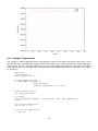
From the data saved, we can obtain the following plot:
In summary, the relax function is useful to obtain a metastable configuration of the system. In particular, it will carry
out the time integration until the remaining torque at any point in the system has dropped below a certain threshold
(Matteo, XXXX, what is this value and where do we set it?).
2.2.6 “Relaxing” the system faster
If we are only interested in the final (meta stable) configuration of a run, we can switch off the precession term in the
Laundau Lifschitz and Gilbert equation. This is done when we define the Material in the following example:
import nmag
from nmag import SI,every,at
mat_Py = nmag.MagMaterial( name="Py",
Ms=SI(0.86e6,"A/m"),
exchange_coupling=SI(13.0e-12, "J/m"),
llg_damping=SI(0.5,""),
do_precession=False)
sim = nmag.Simulation("bar_relax2")
sim.load_mesh("bar30_30_100.nmesh.h5", [("Py", mat_Py)],
unit_length=SI(1e-9,"m"))
sim.set_m([1,0,1])
s = SI("s")
#get SI dimensions for seconds
sim.relax(save = [(’averages’, every(’time’,5e-12*s)),
(’fields’, at(’convergence’))])
2
The integrator (here Sundials) would have to do an extra step to get to the requested time, and if the current time is
close to the requested time, it will simply report this value.
20
The new command is do_precession=False in the constructor of the Permalloy variable mat_Py. As a result, there
will be no precession in the equation of motion:
While the time-development of the system happens at the same time scale as for the system with the precession
term (see “Relaxing” the system), the computation of the system without the precession is significantly faster (for this
example, we needed about 3500 iterations with the precession term and 1500 without it, and the computation time
scales similarly).
Note, that the ”dynamics” shown here are of course artifical and only used to obtain a meta-stable configuration more
efficiently.
2.3 Example: Hysteresis loop for Stoner-Wohlfarth particle
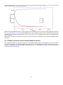
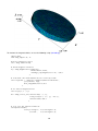
This example computes the hysteresis loop of an ellipsoidal magnetic object, and compares the results with the
analytical solution given by the Stoner-Wohlfahrt model. We use an ellipsoid with semi-axes dimensions of 3 nm, 1
nm and 1 nm along the x, y and z direction, respectively (the mesh is contained in ellipsoid.nmesh.h5 and produced
with Netgen from ellipsoid.geo):
21
2.3.1 Hysteresis simulation script
To compute the hysteresis loop for the ellipsoid, we use the following script (ellipsoid.py):
import nmag
from nmag import SI, at
#create simulation object
sim = nmag.Simulation()
# define magnetic material
Py = nmag.MagMaterial( name="Py",
Ms=SI(1e6,"A/m"),
exchange_coupling=SI(13.0e-12, "J/m")
)
# load mesh: the mesh dimensions are scaled by 100nm
sim.load_mesh( "ellipsoid.nmesh.h5",
[("ellipsoid", Py)],
unit_length=SI(0.5e-9,"m")
)
# set initial magnetisation
sim.set_m([1.,1.,0.])
22
Hs = nmag.vector_set( direction=[1.,1.,0.],
norm_list=[1000.0, 995.0, [], -1000.0,
-995.0, -990.0, [], 1000.0],
units=1e3*SI(’A/m’)
)
# loop over the applied fields Hs
sim.hysteresis(Hs,
save=[(’averages’, at(’convergence’)),
(’fields’,
at(’convergence’))]
)
To execute this script, we call the nsim executable, for example (on linux):
user@host user> nsim ellipsoid.py
As in the previous examples, we first need to import the modules necessary for the simulation, define the material of
the magnetic object, load the mesh and set the initial configuration of the magnetisation as well as the external field.
2.3.2 Hysteresis loop computation
Assume we’d like to apply magnetic fields with a strength of 1e6 A/m down to -1e6 A/m in the [110] direction (i.e. 45
degrees between the x and the y-axis), in steps of 5e3 A/m.
To convey this information efficiently to nmag, we use:
1. a direction for the applied field (here just [1,1,0])
2. a list of magnitudes of the field (this is H_norms) that will be multiplied with the direction vector
3. another multiplier that defines the strength of the applied fields (here 1e3*SI(’A/m’)).
Putting all this together, we obtain this command:
Hs = nmag.vector_set( direction=[1,1,0],
norm_list=[1000.0, 995.0, [], -1000.0,
-995.0, -990.0, [], 1000.0],
units=1e3*SI(’A/m’)
)
which computes a list of vectors Hs. Each entry in the list corresponds to one applied field.
The hysteresis command takes this list of applied fields Hs as one input parameter, and will compute the hysteresis
loop for these fields:
sim.hysteresis(Hs,
save=[(’averages’, at(’convergence’)),
(’fields’,
at(’convergence’))]
)
The second parameter (save) is used to tell the hysteresis command what data to save, and how often. We have come
across this notation when explaining the relax command in the section “Relaxing” the system. In the example shown
here, we request that the averages of the fields should be saved at the point in time where we reach convergence.
We also request that the spatially resolved fields should be saved at convergence.
The hysteresis command computes the time development of the system for one applied field until a convergence
criterion is met. It then proceeds to the next external field value provided during Hs. The value for stopping_dm_dt
which is used as the convergence criterion (see Timestepper parameter example)
23
2.3.3 Obtaining the hysteresis loop data
Once the calculation has finished, we can plot the graph of the magnetisation (projected along the direction of the
applied field) as a function of the applied field.
The ncol command allows us to extract the data and we redirect it to a text file with name nsim.dat:
ncol ellipsoid time H_ext_0 H_ext_1 H_ext_2 m_Py_0 m_Py_1 m_Py_2 > plot.dat
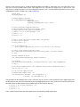
2.3.4 Plotting the hysteresis loop with Gnuplot
Instead of xmgrace (which we have used in Time dependent averages for plotting), other applications can be used.
Here we use Gnuplot:
user@host user> gnuplot make_plot.gnu
which uses the script in make_plot.gnu:
set term postscript enhanced color
set out ’hysteresis.ps’
set xlabel ’Applied field (kA/m)’
set ylabel ’M / Ms’
versor_x = 0.707106781186548
versor_y = 0.707106781186548
versor_z = 0.0
scalar_prod(x1,x2,x3) = (x1*versor_x+x2*versor_y+x3*versor_z)
magnit(x1,x2,x3) = sqrt(x1*x1+x2*x2+x3*x3)
plot [-1050:1050] [1.2:1.2] ’plot.dat’ u (scalar_prod($1,$2,$3)/1000):(scalar_prod($4,$5,$6)) ti ’StonerWohlfahrt’ w lp 4
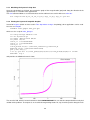
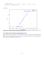
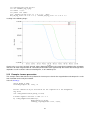
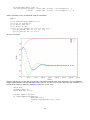
and provides the following hysteresis loop:
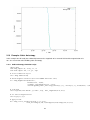
The coercive field, which is located somewhere between 165 and 170 kA/m, can now be compared with an analytical
solution of the problem. To compute it, we need the demagnetizing factors Nx, Ny, Nz of the particle along the main
24
axes. Since we deal with a prolate ellipsoid where two of the axes have the same dimension ( y and z in this case), it
is sufficient to compute the factor along the longest axis (x axis), and the other two are easily derived from the relation
Nx + Ny + Nz = 1. The expression to compute the Nx is the following
where, calling a the length of the particle semi-axis along the x direction and c the length of the semi-axis along the
y (or z) direction, m is defined as m = a/c. The value of Nx is therefore 0.1087, while the others are Ny = Nz = 0.4456
from the equation Nx + Ny + Nz = 1. With these values the shape anisotropy is easily computed according to the
expression
which gives Ha = 337 kA/m in the case of Ms = 1000 kA/m. The final step is to compute the coercive field hc using
the following analytical result (Stoner-Wohlfahrt model):
where theta_0 is the angle between the easy-axis of the particle (x-axis in our case) and the direction of the applied
field. Substituting theta_0 = 45 (degrees) in the formula, we obtain hc = 0.5, that is Hc = 0.5 * Ha = 168 kA/m. As
we have seen before, the simulated hysteresis loop gives a value between 165 and 170 kA/m, which is in agreement
with the analytical solution.
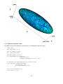
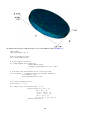
2.4 Example: Hysteresis loop for thin disk
This example computes the hysteresis loop of a flat disc magnetised along a direction orthogonal to the main axis. In
comparison to the previous Stoner-Wohlfarth example, it shows use a more complex sequence of applied fields.
We use a disc 10 nm thick and 200 nm in diameter for this example (the mesh is contained in nanodot.nmesh.h5
which is created from nanodot1.geo with Netgen):
25
To compute the hysteresis loop for the disc, we use the following script (nanodot1.py):
import nmag
from nmag import SI, at
#create simulation object
sim = nmag.Simulation()
# define magnetic material
Py = nmag.MagMaterial( name="Py",
Ms=SI(795774,"A/m"),
exchange_coupling=SI(13.0e-12, "J/m")
)
# load mesh: the mesh dimensions are scaled by 100nm
sim.load_mesh( "../example_hysteresis/cylinder1.nmesh.h5",
[("cylinder", Py)],
unit_length=SI(100e-9,"m")
)
# set initial magnetisation
sim.set_m([1.,0.,0.])
Hs = nmag.vector_set( direction=[1.,0.,0.],
norm_list=[1000.0, 900.0, [],
95.0, 90.0, [],
-100.0, -200.0, [],
-1000.0, -900.0, [],
-95.0, -90.0, [],
100.0, 200.0, [], 1000.0],
units=1e3*SI(’A/m’)
)
26
# loop over the applied fields Hs
sim.hysteresis(Hs,
save=[(’averages’, at(’convergence’)),
(’fields’,
at(’convergence’)),
#
(’restart’, at(’convergence’)) # not working yet
]
)
We assume that the previous example have been sufficiently instructive to explain the basic steps such as importing
nmag, creating a simulation object, defining the material and leading the mesh. We focus on the hysteresis command:
We’d like to apply fields ranging from [1e6, 0, 0] A/m to [100e3, 0, 0] A/m in steps of 100e3 A/m.
Then from [95e3, 0, 0] A/m to [-95e3, 0, 0] A/m we would like to use a smaller step size of 5e3 A/m (to resolve
this applied field range better).
This will take us through zero applied field ([0,0,0] A/m). Now, symmetric to the positive field values, we would like
to use a step size of 100e3 A/m again to go from [-100e3, 0, 0] A/m to [1e6, 0, 0] A/m. At this point, we would
like to reverse the whole sequency (to sweep the field back to the initial value).
The information we need for the hysteresis command includes:
1. a direction for the applied field (here just [1,0,0])
2. a list of magnitudes of the field (this is the norm_list) that will be interpreted, and then multiplied with the
direction vector.
As in the Stoner-Wohlfarth example, the input provided here is interpreted. For example, the expression:
[1000.0, 900.0, [],
95.0]
means that we start with a magnitude of 1000, the next magnitude is 900. The empty brackets ([])
indicate that this sequence should be continued (i.e. 800, 700, 600, 500, 400, 300, 200, 100) until the
next value given is reached (i.e. 95).
3. another multiplier that defines the strength of the applied fields (here 1e3*SI(’A/m’)).
The corresponding command is:
Hs = nmag.vector_set( direction=[1,0,0],
norm_list=[1000.0, 900.0, [],
95.0, 90.0, [],
-100.0, -200.0, [],
-1000.0, -900.0, [],
-95.0, -90.0, [],
100.0, 200.0, [], 1000.0],
units=1e6*SI(’A/m’)
)
which computes a list of vectors Hs. The hysteresis command takes this list of applied fields Hs as one input parameter, and will compute the hysteresis loop for these fields:
sim.hysteresis(Hs,
save=[(’averages’, at(’convergence’)),
(’fields’,
at(’convergence’)),
(’restart’, at(’convergence’))
]
)
Again, the second parameter (save) is used to tell the hysteresis command what data to save, and how often. We
request that the averages of the fields should be saved at the point in time where we reach convergence. We also
request that the spatially resolved fields should be saved at convergence. We further request that restart data is
saven at convergence (see restart example).
27
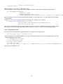
2.4.1 Thin disk hysteresis loop
Once the calculation has finished, we can plot the hysteresis loop, i.e. the graph of the magnetisation computed
along the direction of the applied field as a function of the applied field.
The ncol command allows us to extract the data and we redirect it to a text file with name plot.dat:
ncol nanodot1 H_ext_0 m_Py_0 > plot.dat
which saves the file plot.dat which starts as following:
1000000
950000
900000
850000
800000
0.9999551243645
0.9999541970431
0.9999531184538
0.9999519886171
0.999950827041
We use Gnuplot to plot the hysteresis loop:
user@host user> gnuplot make_plot.gnu
which uses the script in make_plot.gnu:
set term postscript enhanced color
set out ’nanodot_hyst.ps’
set xlabel ’Applied field (A/m)’
set ylabel ’M / Ms’
plot [-1.2e6:1.2e6] [-1.2:1.2] ’nmag.dat’ u 2:3 ti ’nmag’ with linespoints lw 3 pt 5
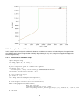
The resulting graph is shown here:
and the comparison with the magpar data, obtained with the script make_comparison_plot.gnu:
set term postscript enhanced color
set out ’nanodot_hyst.ps’
set xlabel ’Applied field (A/m)’
28
set ylabel ’M / Ms’
plot [-0.2e3:0.2e3] [-1.2:1.2] ’nmag.dat’ u ($2/1000):3
par.dat’ u 3:4 ti ’magpar’ w lp 4
ti ’nmag’ w lp 3, ’mag-
is shown here:
Here we can see the different switching point between nmag and magpar, probably due to different tolerances in the
estimation of the convergence for the time integrator in the two cases.
2.5 Example: Vortex formation and propagation in disk
This example computes the evolution of a vortex in a flat cylinder magnetised along a direction orthogonal to the main
axis.
We use a flat the same geometry as in the Hysteresis loop for thin disk example: cylinder, 10 nm thick and 200 nm in
diameter (the mesh is contained in nanodot.nmesh.h5):
29
To simulate the magnetised disc, we use the following script (nanodot.py):
import nmag
from nmag import SI, at
#create simulation object
sim = nmag.Simulation()
# define magnetic material
Py = nmag.MagMaterial( name="Py",
Ms=SI(795774,"A/m"),
exchange_coupling=SI(13.0e-12, "J/m")
)
# load mesh: the mesh dimensions are scaled by 100nm
sim.load_mesh( "../nanodot_comparison/nanodot.nmesh.h5",
[("cylinder", Py)],
unit_length=SI(100e-9,"m")
)
# set initial magnetisation
sim.set_m([1.,0.,0.])
Hs = nmag.vector_set( direction=[1.,0.,0.],
norm_list=[12.0, 7.0, [], -200.0],
units=1e3*SI(’A/m’)
)
# loop over the applied fields Hs
sim.hysteresis(Hs,
save=[(’averages’, at(’convergence’)),
(’fields’,
at(’convergence’)),
30
#
(’restart’,
at(’convergence’)) # not working yet
]
)
We would like to compute the magnetisation behaviour in the applied fields ranging from [12e3, 0, 0] A/m to [200e3, 0, 0] A/m in steps of 5e3 A/m. The command for this is:
Hs = nmag.vector_set( direction=[1,0,0],
norm_list=[12.0, 7.0, [], -200.0],
units=1e3*SI(’A/m’)
)
sim.hysteresis(Hs,
save=[(’averages’, at(’convergence’)),
(’fields’,
at(’convergence’)),
]
)
Once the calculation has finished, we can plot the evolution of the magnetisation, i.e. the graph of the magnetisation
computed along the direction of the applied field as a function of the applied field.
The ncol command allows us to extract the data and we redirect it to a text file with name nsim.dat:
ncol nanodot time H_ext_0 m_Py_0 m_Py_1 m_Py_2 > plot.dat
Plotting the data with Gnuplot:
user@host user> gnuplot make_plot.gnu
which uses the script in make_plot.gnu:
set term postscript enhanced color
set out ’nanodot_evo.ps’
set xlabel ’Applied field (A/m)’
set ylabel ’M / Ms’
plot [-250:50] [-1.2:1.2] ’nsim.dat’ u ($2/1000):3
par.dat’ u ($1>0 ? $3 : 1/0):4 ti ’magpar’ w lp 4
The resulting graph is shown here:
31
ti ’nsim’ w lp 3 #, ’mag-
and we can see that the results from nsim match those from magpar . The magnetization configuration during the
switching process are shown in the following snapshots:
Figure 1: Magnetisation configuration for a decreasing applied field of 20 kA/m.
We see that during magnetisation reversal a vortex nucleates on the boundary of the disc when the field is sufficiently
decreased from its saturation value. As the field direction is aligned with the x-axis, the vortex appears in the disc
region with the largest y component, and it moves downwards towards the centre along the y-axis. With a further
decrease of the applied field the vortex moves towards the opposite side of the disc with respect to the nucleation
32
Figure 2: Magnetisation configuration for a decreasing applied field of 15 kA/m.
Figure 3: Magnetisation configuration for a decreasing applied field of 10 kA/m.
33
Figure 4: Magnetisation configuration for a decreasing applied field of -30 kA/m.
Figure 5: Magnetisation configuration for a decreasing applied field of -95 kA/m.
34
Figure 6: Magnetisation configuration for a decreasing applied field of -100 kA/m.
position, and it is eventually expelled when the magnetisation aligns with the field direction over all the disc.
2.6 Example: Manipulating magnetisation
The basics of this file are as in Example: Demag field in uniformly magnetised sphere: a ferromagnetic sphere is studied, and initially configured to have homogeneous magnetisation. Here is the source code of sphere_manipulate.py
import nmag4 as nmag
from nmag4 import SI
#create simulation object
sim = nmag.Simulation()
# define magnetic material
Py = nmag.MagMaterial(name="Py",
Ms=SI(1e6,"A/m"),
exchange_coupling=SI(13.0e-12, "J/m")
)
# load mesh
sim.load_mesh("sphere1.nmesh.h5", [("sphere", Py)], unit_length=SI(1e-9,"m") )
# set initial magnetisation
sim.set_m([1,0,0])
# set external field
sim.set_H_ext([0,0,0],SI(1,"A/m"))
# Save and display data in a variety of ways
# Step 1: save all fields spatially resolved
35
sim.save_data(fields=’all’)
# Step 2: sample demag field through sphere
for i in range(-10,11):
x = i*1e-9
#position in metres
H_demag = sim.probe_subfield_f( ’H_demag’, [x,0,0] )
print "x =", x, ": H_demag = ", H_demag
# Step 3: sample exchange field through sphere
for i in range(-10,11):
x = i*1e-9
#position in metres
H_exch_Py = sim.probe_subfield_f( ’H_exch_Py’, [x,0,0] )
print "x =", x, ": H_exch_Py = ", H_exch_Py
#now modify the magnetisation at position (0,0,0) (this happens to be
#node 0 in the mesh.)
#Step 4: request a vector with the magnetisation of all sites in the
#mesh
myM = sim.get_subfield(’m_Py’)
#Step 5: We modify the first entry:
myM[0] = [0,1,0]
#Step 6: Set the magnetisation to the new (modified) values
sim.set_m(myM)
#Step 7: saving the fields again (so that we can later plot the demag
#and exchange field
sim.save_data(fields=’all’)
#Step 8: sample demag field through
for i in range(-10,11):
x = i*1e-9
H_demag = sim.probe_subfield_f(
print "x =", x, ": H_demag = ",
sphere
#position in metres
’H_demag’, [x,0,0] )
H_demag
#Step 9: sample exchange field through sphere
for i in range(-10,11):
x = i*1e-9
#position in metres
H_exch_Py = sim.probe_subfield_f( ’H_exch_Py’, [x,0,0] )
print "x =", x, ": H_exch_Py = ", H_exch_Py
To execute this script, we have to give its name to the nsim executable, for example (on linux):
user@host user> nsim sphere_manipulate.py
Let us discuss the sphere_manipulate.py script step by step. After having created the simulation object, defined the
material, loaded the mesh, set the initial magnetisation and the external field, we save the data the first time (Step 1).
We could visualise the magnetisation and all other fields as described in Example: Demag field in uniformly magnetised sphere, and would obtain the same figures as shown in section Saving spatially resolved data.
In step 2, we probe the demag field at positions along a line going from [-10,0,0]nm to [10,0,0]nm, and then print the
values. This produces the following output:
x = -1e-08 : H_demag =
None
36
x
x
x
x
x
x
x
x
x
x
x
x
x
x
x
x
x
x
x
x
=
=
=
=
=
=
=
=
=
=
=
=
=
=
=
=
=
=
=
=
-9e-09
-8e-09
-7e-09
-6e-09
-5e-09
-4e-09
-3e-09
-2e-09
-1e-09
0.0
1e-09
2e-09
3e-09
4e-09
5e-09
6e-09
7e-09
8e-09
9e-09
1e-08
:
:
:
:
:
:
:
:
:
:
:
:
:
:
:
:
:
:
:
:
H_demag
H_demag
H_demag
H_demag
H_demag
H_demag
H_demag
H_demag
H_demag
H_demag
H_demag
H_demag
H_demag
H_demag
H_demag
H_demag
H_demag
H_demag
H_demag
H_demag
=
=
=
=
=
=
=
=
=
=
=
=
=
=
=
=
=
=
=
=
[-329656.18892701436, 131.69946810517845, 197.13873034397167]
[-329783.31649797881, 68.617197264295427, 140.00328871543459]
[-329842.17628131888, 183.37401011699876, 163.01612229436262]
[-329904.84956877632, 133.62473797637142, 74.090532749764847]
[-329974.43178624194, 85.517390832982983, -13.956465964930704]
[-330002.69224229571, 64.187663119270084, -30.832135394870004]
[-330006.79488959321, 25.479055440690821, -61.958073893954818]
[-330020.18327401817, 11.70722487517595, -58.143562276077219]
[-330025.52325345919, -5.7120648683347452, -52.237341988696294]
[-330028.67095553532, -25.707310077918752, -46.346108473560378]
[-330058.98559210222, -37.699378078580203, -41.167364094137213]
[-330089.30022866925, -49.691446079241658, -35.988619714714041]
[-330145.36618529289, -63.819285767062581, -22.213920341440794]
[-330220.13307247689, -76.54950394725968, -5.0509172407556262]
[-330298.69089200837, -90.534514175273259, 13.57279800234617]
[-330375.34327985492, -117.01128011426778, 35.262477275758371]
[-330415.38940687838, -123.68558207391983, 60.580352625726341]
[-330474.37719032855, -112.22952205433305, 106.13032196062491]
[-330499.64039893239, -69.97070465326442, 160.41688110297264]
[-330518.649930441, -26.536490670368085, 212.32392103651733]
The data is approximately 1/3 Ms = 333333 in the direction of the magnetisation, and approximately zero in the other
directions, as we would expect in a homogenously magnetised sphere. The deviations we see are due to (i) the shape
of the sphere not being perfectly resolved (ie we actually look at the demag field of a polyhedron) and (ii) numerical
errors.
In step 3, we probe the exchange field along the same line. The exchange field is effectively zero because the
magnetisation is pointing everywhere in the same direction:
x
x
x
x
x
x
x
x
x
x
x
x
x
x
x
x
x
x
x
x
x
=
=
=
=
=
=
=
=
=
=
=
=
=
=
=
=
=
=
=
=
=
-1e-08
-9e-09
-8e-09
-7e-09
-6e-09
-5e-09
-4e-09
-3e-09
-2e-09
-1e-09
0.0
1e-09
2e-09
3e-09
4e-09
5e-09
6e-09
7e-09
8e-09
9e-09
1e-08
:
:
:
:
:
:
:
:
:
:
:
:
:
:
:
:
:
:
:
:
:
H_exch_Py
H_exch_Py
H_exch_Py
H_exch_Py
H_exch_Py
H_exch_Py
H_exch_Py
H_exch_Py
H_exch_Py
H_exch_Py
H_exch_Py
H_exch_Py
H_exch_Py
H_exch_Py
H_exch_Py
H_exch_Py
H_exch_Py
H_exch_Py
H_exch_Py
H_exch_Py
H_exch_Py
=
=
=
=
=
=
=
=
=
=
=
=
=
=
=
=
=
=
=
=
=
None
[-1.264324643856989e-09, 0.0, 0.0]
[-2.0419540595507732e-10, 0.0, 0.0]
[-1.4334754136843496e-09, 0.0, 0.0]
[-2.7214181426130964e-10, 0.0, 0.0]
[1.6323042074911775e-09, 0.0, 0.0]
[-1.6243345875473033e-09, 0.0, 0.0]
[-5.6526341264934703e-09, 0.0, 0.0]
[-6.1145979552370084e-09, 0.0, 0.0]
[-3.0929969691649876e-09, 0.0, 0.0]
[9.2633407053741312e-10, 0.0, 0.0]
[1.9476821552904271e-09, 0.0, 0.0]
[2.9690302400434413e-09, 0.0, 0.0]
[2.6077357277001043e-09, 0.0, 0.0]
[1.5836815585162886e-09, 0.0, 0.0]
[1.6602158583197139e-09, 0.0, 0.0]
[1.8844573960991853e-09, 0.0, 0.0]
[-6.2460015649740799e-09, 0.0, 0.0]
[-1.1231714572170603e-08, 0.0, 0.0]
[-7.3643182171284044e-09, 0.0, 0.0]
[-3.4351784609779937e-09, 0.0, 0.0]
Note that the subfield name we are probing for the exchange field is H_exch_Py whereas the subfield name we
used to probe the demag field is H_demag (without the extension _Py. The reason for this is that the exchange field
is a something that is associated with a particular material (here Py) whereas the is only one demag field that is
experienced by all materials.
2.6.1 Modifying the magnetisation
In step 4, we use the get_subfield command. This will return a (numpy) array that contains one 3d vector for every
site of the finite element mesh.
37
In step 5, we modify the first entry in this array (which has index 0), and set its value to [0,1,0]. Whereas the
magnetisation is pointing everywhere in [1,0,0] (because we have used the set_m command in the very beginning of
the program, it is now pointing in the [0,1,0] at site 0.
The information, which site corresponds to which entry in the data vector we have obtained using get_subfield can be
retrieved from get_subfield_sites. Correspondly, the position of the sites can be obtained using get_subfield_positions.
We now need to set this modified magnetisation vector (Step 6) using the set_m command.
If we save the data again to the file (Step 7), we can subsequently convert this to a vtk file (using, for example, nmagpp
--vtk data sphere_manipulate) and visualise with mayavi:
We can see one blue cone in the centre of the sphere -- this is the one site that he have modified to point in the
y-direction (whereas all other cones point in the x-direction).
As before, we can probe the fields along a line through the center of the sphere (Step 8). For the demag field we
obtain:
x
x
x
x
x
x
x
x
x
x
x
=
=
=
=
=
=
=
=
=
=
=
-1e-08
-9e-09
-8e-09
-7e-09
-6e-09
-5e-09
-4e-09
-3e-09
-2e-09
-1e-09
0.0
:
:
:
:
:
:
:
:
:
:
:
H_demag
H_demag
H_demag
H_demag
H_demag
H_demag
H_demag
H_demag
H_demag
H_demag
H_demag
=
=
=
=
=
=
=
=
=
=
=
None
[-333816.99138074159, -1884.643376396662, 16.665519199152595]
[-334670.87148225965, -2293.608410913705, -102.38526828192296]
[-335258.77403632947, -3061.1708540342884, -532.73877752122235]
[-339506.72150998382, -5316.1506383768137, -969.36630578549921]
[-344177.83909963415, -8732.9787600552572, -1610.433091871927]
[-344725.75257842313, -16708.164927667149, -5224.2484897904633]
[-337963.49070659198, -24567.078937669514, -3321.016613832679]
[-321612.85117992124, -30613.873989917105, -1385.6383061516099]
[-298312.3363571504, -41265.117003123923, 636.60703829516081]
[-273449.78240732534, -52534.176864875568, 2793.5027588779139]
38
x
x
x
x
x
x
x
x
x
x
=
=
=
=
=
=
=
=
=
=
1e-09
2e-09
3e-09
4e-09
5e-09
6e-09
7e-09
8e-09
9e-09
1e-08
:
:
:
:
:
:
:
:
:
:
H_demag
H_demag
H_demag
H_demag
H_demag
H_demag
H_demag
H_demag
H_demag
H_demag
=
=
=
=
=
=
=
=
=
=
[-293644.21931918303,
[-313838.65623104072,
[-330296.09687372146,
[-343611.94111195666,
[-348062.40814087034,
[-342272.36888512014,
[-338716.66400897497,
[-335656.89887674141,
[-334985.59512328985,
[-334441.59096545313,
-39844.049389551074, 4310.6449471266505]
-27153.921914226579, 5827.7871353753881]
-21814.293451835449, 5525.7290665358933]
-18185.932406317523, 4931.5464761658959]
-11029.603829202088, 3781.8263522408147]
-6604.210117819096, 50.151907623841332]
-3860.7761876767272, 485.90273674867018]
-2610.0345208853882, 586.74812908870092]
-2169.9546280837162, 542.76746044672041]
-1634.8337299563193, 627.17874011463311]
The change of the magnetisation at position [0,0,0] from [1,0,0] to [0,1,0] has reduced the x-component of the demag
field somewhat around x=0, and has introduced a significant demag field in the -y direction around x=0.
Looking at the exchange field (Step 9):
x
x
x
x
x
x
x
x
x
x
x
x
x
x
x
x
x
x
x
x
x
=
=
=
=
=
=
=
=
=
=
=
=
=
=
=
=
=
=
=
=
=
-1e-08 :
-9e-09 :
-8e-09 :
-7e-09 :
-6e-09 :
-5e-09 :
-4e-09 :
-3e-09 :
-2e-09 :
-1e-09 :
0.0
:
1e-09 :
2e-09 :
3e-09 :
4e-09 :
5e-09 :
6e-09 :
7e-09 :
8e-09 :
9e-09 :
1e-08 :
H_exch_Py
H_exch_Py
H_exch_Py
H_exch_Py
H_exch_Py
H_exch_Py
H_exch_Py
H_exch_Py
H_exch_Py
H_exch_Py
H_exch_Py
H_exch_Py
H_exch_Py
H_exch_Py
H_exch_Py
H_exch_Py
H_exch_Py
H_exch_Py
H_exch_Py
H_exch_Py
H_exch_Py
=
=
=
=
=
=
=
=
=
=
=
=
=
=
=
=
=
=
=
=
=
None
[-1.264324643856989e-09, 0.0, 0.0]
[-2.0419540595507732e-10, 0.0, 0.0]
[-1.4334754136843496e-09, 0.0, 0.0]
[-2.7214181426130964e-10, 0.0, 0.0]
[1.6323042074911775e-09, 0.0, 0.0]
[-153858.81305452777, 153858.81305452611, 0.0]
[-972420.67935341748, 972420.67935341166, 0.0]
[-2445371.8369108676, 2445371.8369108611, 0.0]
[5283169.701234119, -5283169.7012341227, 0.0]
[15888993.991894867, -15888993.991894867, 0.0]
[8434471.7912872285, -8434471.7912872266, 0.0]
[979949.59067958547, -979949.59067958279, 0.0]
[-1112837.3087986181, 1112837.3087986207, 0.0]
[-193877.66176242317, 193877.6617624248, 0.0]
[1.6602158583197139e-09, 0.0, 0.0]
[1.8844573960991853e-09, 0.0, 0.0]
[-6.2460015649740799e-09, 0.0, 0.0]
[-1.1231714572170603e-08, 0.0, 0.0]
[-7.3643182171284044e-09, 0.0, 0.0]
[-3.4351784609779937e-09, 0.0, 0.0]
We can see that the exchange field is indeed very large around x=0.
Note that one of the fundamental problem of micromagnetic simulations is that the magnetisation must not vary
significantly from one site to another. In this example, we have manually violated this requirement only to demonstrate
how the magnetisation can be modified, and to see that this is reflected in the dependant fields (such as demag and
exchange) immediately.
2.7 Example: IPython
The basics of this file are as in Example: Demag field in uniformly magnetised sphere: a ferromagnetic sphere is
studied, and initially configured to have homogeneous magnetisation.
Here is the source code of sphere_ipython.py
import nmag4 as nmag
from nmag4 import SI
#create simulation object
sim = nmag.Simulation()
# define magnetic material
Py = nmag.MagMaterial(name="Py",
Ms=SI(1e6,"A/m"),
39
exchange_coupling=SI(13.0e-12, "J/m")
)
# load mesh
sim.load_mesh("sphere1.nmesh.h5", [("sphere", Py)], unit_length=SI(1e-9,"m") )
# set initial magnetisation
sim.set_m([1,0,0])
nmag.ipython()
To execute this script, we have to give its name to the nsim executable, for example (on linux):
user@host user> nsim sphere_ipython.py
The new command appearing here is nmag.ipython() in the last line.
This calls an interactive python interpreter (this is like the standard ipython interpreter called from the command
prompt).
Once we are “inside” this interpreter, we can interactively work with the simulation object. We demonstrate this with
the transcript of such a session:
user@host user> nsim sphere_ipython.py
<snip>
In [1]: sim.get_subfield("H_demag")
Out[1]:
array([[ -3.30028671e+05, -2.57073101e+01,
[ -3.30518650e+05, -2.65364907e+01,
[ -3.30380750e+05, -1.34382835e+02,
...,
[ -3.30063839e+05,
4.56312711e+01,
[ -3.30056243e+05, -3.23341645e+01,
[ -3.29950815e+05,
4.44150291e+01,
-4.63461085e+01],
2.12323921e+02],
1.94635283e+01],
-1.31204248e+02],
-2.26732582e+02],
-5.41700794e+01]])
In [2]: sim.set_m([0,0,1])
In [3]: sim.get_subfield("H_demag")
Out[3]:
array([[ -6.86773473e+01,
4.44496808e+01,
[ -2.83792944e+02,
1.78935681e+02,
[ -2.04396266e+02,
2.48374212e+02,
...,
[ -1.02055030e+02, -9.53215211e+01,
[ 1.94875407e+02,
1.22757584e+02,
[ 6.16259262e+01,
1.66071597e+02,
-3.30084368e+05],
-3.30268314e+05],
-3.30180923e+05],
-3.30239401e+05],
-3.29771010e+05],
-3.29848851e+05]])
Note that within ipython, one can just press the TAB key to autocomplete object names, funtions and commands.
You can leave the ipython enviroment by pressing CTRL+D. For the script shown here, this will stop the execution.
2.8 Example: Pinning Magnetisation
In this example we show how to pin (i.e. fix) magnetisation in certain parts of a material.
2.8.1 Pinning simulation script
import nmag
40
from nmag import SI, si
# create simulation object
sim = nmag.Simulation()
# define magnetic material: PermAlloy
Py = nmag.MagMaterial(name="Py",
Ms=SI(0.86e6,"A/m"),
exchange_coupling=SI(13.0e-12, "J/m"))
# load mesh
sim.load_mesh("sphere1.nmesh.h5", [("sphere", Py)], unit_length=SI(1e-9,"m") )
# set initial magnetisation to +x direction
sim.set_m([1,0,0])
# pin magnetisation at center in radius of 4e-9m
def pin_at_center((x,y,z)):
if (x*x + y*y + z*z) < (4e-9)*(4e-9):
return 0.0 #inside the 4nm sphere -> pin
else:
return 1.0 #outside -> do not pin
sim.set_pinning(pin_at_center)
# apply external field in +y direction
unit = 0.5*si.T/si.mu0 #500mT in A/m
sim.set_H_ext([0*unit, 1*unit, 0*unit])
# relax the magnetisation
sim.relax()
We will now discuss the sphere.py example step-by-step:
We first define a material modelling Permalloy and apply it to a sphere with radius 10 nm. Then we set initial
magnetisation to point in +x direction.
2.8.2 Pinning magnetisation
In order to allow the user to fix magnetisation, nmag provides a scalar field, the so-called pinning field: its value at
each site is used as a scale factor for dm/dt, hence by setting it to 0 at certain locations of the mesh we can force
magnetisation to remain constant at these locations for the entire simulation.
We now set the pinning field using set_pinning (which is used like set_m and set_H_ext, except that it is a scalar field
whereas the latter are vector fields) such that magnetisation is fixed at sites with distance less than 4 nm from the
sphere’s center. First we define a Python function which we decide to call pin_at_center:
def pin_at_center((x,y,z)):
if (x*x + y*y + z*z) < (4e-9)*(4e-9):
return 0.0
else:
return 1.0
The function receives a 3-tuple ((x,y,z)) containing the three floating point variables x, y and z provide the position
coordinates (in metres) for which the function returns either 0.0 (which means the magnetisation at this position is
pinned) or 1.0 (in which case there is no pinning). The formula in the if statement simply evaluates the Cartesian
magnitude of the vector [x,y,z] by squaring each component. This number is then compared against (4nm)^2. As
a result, all the nodes (i.e. corners of tetrahedra) that are located within a sphere with radius 4nm are pinned, and all
nodes that are located outside this sphere can change as usual.
Second, we need to tell nmag that it should use this function to decide where the magnetisation should be pinned:
41
sim.set_pinning(pin_at_center)
Note the slightly counterintuitive fact that value 1 means “no pinning”.
Finally we apply an external field of half a Tesla in +y direction, and use relax to compute the equilibrium configuration.
2.8.3 Visualisation
After running the example via nsim sphere.py we convert the equilibrium data to VTK format:
nmagpp --vtk=sphere.vtk sphere
We would first like to verify that the pinning field has been set up properly. Hence we use MayaVi to visualize it by
showing an isosurface of the pinning field (shown as blue).
The blue blob in the center of the sphere is the collection of those tetrahedra that have corners just inside the 4nm
sphere. Because we have not generated the mesh to have nodes coinciding with the 4nm sphere, the shape of the
blue region is not particularly spherical.
We further show the magnetisation vectors of the final configuration. Their colour corresponds to the pinning field
at their location. It can be seen that the blue magnetisation vectors emerging from the central region of the sphere,
are all pointing (strictly) in the x-direction. The magnetisation vectors outside the blue sphere are coloured red. The
applied field drives these vectors to point into the y-direction. However, the magnetisation in the centre is pinned and
the exchange interaction requires a gradual spatial change of magnetisation. This explains the spatial variation of the
magnetisation.
42
The next figure, shows the same data is the last one but in addition a ScalarCutPlane (in MayaVi terminology) has
been introduced which is coloured according to the x-component of the magnetisation. Red corresponds to 1.0 and
blue corresponds to 0.73 (we have not shown the legend to provide a larger main plot). This demonstrates the gradual
change from the pinned magnetisation in the centre to the outside.
2.9 Example: Uniaxial anisotropy
In this example we would like to simulate the development of a Bloch type domain wall on a thin cobalt bar of
dimension 504 x 1 x 1 nm (bar.nmesh.h5) due to uniaxial anisotropy.
2.9.1 Unixaial anisotropy simulation script
import nmag
from nmag import SI, every, at
from numpy import array
from math import sin, cos, pi, sqrt
# create simulation object (no demag field!)
sim = nmag.Simulation(do_demag=False)
# define magnetic material (data from OOMMF materials file)
Co = nmag.MagMaterial(name="Co",
43
Ms=SI(1400e3, "A/m"),
exchange_coupling=SI(30e-12, "J/m"),
anisotropy=nmag.uniaxial_anisotropy(axis=[0,0,1], K1=SI(520e3, "J/m^3")))
# load mesh
sim.load_mesh("bar.nmesh.h5", [("bar", Co)], unit_length=SI(1e-9,"m") )
# set initial magnetisation
def sample_m0((x,y,z)):
if x<=2e-9:
return [0,0,1]
if x>=502e-9:
return [0,0,-1]
z = -2*(x-2e-9)/500e-9+1
return [0, sqrt(1-z*z), z]
sim.set_m(sample_m0)
# pin lhs/rhs magnetisation
def sample_pinning((x,y,z)):
return x>=2e-9 and x<=502e-9
sim.set_pinning(sample_pinning)
# save magnetisation along x axis
def save_magnetisation_along_x(filename):
f = open(filename, ’w’)
for i in range(0, 504):
x = array([i+0.5,0.5,0.5]) * 1e-9
M = sim.probe_subfield_f(’M_Co’, x)
print >>f, x[0], M[0], M[1], M[2]
# simulate
dt = SI(1e-9, "s")
for i in range(0, 11):
sim.advance_time(i*dt)
save_magnetisation_along_x(’bar_mag_x_%02ins.txt’ % i)
We shall now discuss the bar.py script step-by-step:
In this particular example we are solely interested in energy terms resulting from exchange interaction and anisotropy.
Hence we disable the demagnetisation field as follows:
sim = nmag.Simulation(do_demag=False)
We then create the Co material modelling cobalt exhibiting uniaxial anisotropy in z direction with phenomenological
anisotropy constant K1 = SI(520e3, "J/m^3"):
Co = nmag.MagMaterial(name="Co",
Ms=SI(1400e3, "A/m"),
exchange_coupling=SI(30e-12, "J/m"),
anisotropy=nmag.uniaxial_anisotropy(axis=[0,0,1], K1=SI(520e3, "J/m^3")))
After loading the mesh, we set the initial magnetisation direction such that it rotates from +z to -z while staying in the
plane normal to x direction (hence suggesting the development of a Bloch type domain wall):
def sample_m0((x,y,z)):
if x<=2:
return [0,0,1]
if x>=502:
44
return [0,0,-1]
z = -2*(x-2.0)/500+1
return [0, sqrt(1-z*z), z]
We further pin magnetisation at the very left and right of the bar:
# pin lhs/rhs magnetisation
def sample_pinning((x,y,z)):
return x>=2 and x<=502
sim.set_pinning(sample_pinning)
Finally, we compute the system’s time development for 10 nanoseconds, saving magnetisation spatially resolved
along the x axis in a format understandable by Gnuplot.
2.9.2 Visualization
We can then use Gnuplot to visualize magnetisation after 10 nanoseconds using the following script:
set term png giant size 800,600
set out ’bar_mag_x_10ns.png’
set xlabel ’x (nm)’
set ylabel ’M.z (A/m)’
plot [0e-9:502e-9] [-1400e3:1400e3] ’bar_mag_x_10ns.txt’ u 1:4 ti ’nmag’ w l 2
The resulting plot clearly shows that a Bloch type domain wall has developed:
2.9.3 Comparison
After simulating the same scenario with OOMMF (see ../example_uniaxial_anis/oommf/bar.mif), we can compare
results using another Gnuplot script:
45
set term png giant size 800,600
set out ’bar_mag_x_10ns_vs_oommf.png’
set xlabel ’x (nm)’
set ylabel ’M.z (A/m)’
plot [0e-9:502e-9] [1400e3:1400e3] ’bar_mag_x_10ns.txt’ u 1:4 ti ’nmag’ w l 2, ’oommf/bar_mag_x.txt’ u 1:4 ti ’oommf’ w l
which generates the following plot showing good agreement of both systems:
We also remark that the nmag result almost perfectly matches the analytical solution given by cos(atan(sinh((xx_wall)/sqrt(A/K1)))+pi/2)*Ms:
46
2.10 Example: Cubic Anisotropy
In this example we will study the relationship between the magnitude of an external field and the magnetisation of a
10 x 10 x 10 nm iron cube exhibiting cubic anisotropy.
2.10.1 Cubit anisotropy simulation script
import nmag
from nmag import SI, every, at, si
from math import sin, cos, pi, sqrt
# create simulation object
sim = nmag.Simulation()
# define magnetic material (data from OOMMF materials file)
Fe = nmag.MagMaterial(name="Fe",
Ms=SI(1700e3, "A/m"),
exchange_coupling=SI(21e-12, "J/m"),
anisotropy=nmag.cubic_anisotropy(axis1=[1,0,0], axis2=[0,1,0], K1=SI(48e3, "J/m
# load mesh
sim.load_mesh("cube.nmesh", [("cube", Fe)], unit_length=SI(1e-9,"m"))
# set initial magnetisation
sim.set_m([0,0,1])
# apply fields
Hs = nmag.vector_set(direction=[1.0,0,0.0001],
norm_list=range(0,191,10)+range(191,211)+range(210,501,10),
47
units=0.1*0.001*si.T/si.mu0)
sim.hysteresis(Hs)
We will now discuss the cube.py script step-by-step:
After creating the simulation object we define a magnetic material Fe with cubic anisotropy representing iron:
Fe = nmag.MagMaterial(name="Fe",
Ms=SI(1700e3, "A/m"),
exchange_coupling=SI(21e-12, "J/m"),
anisotropy=nmag.cubic_anisotropy(axis1=[1,0,0], axis2=[0,1,0], K1=SI(48e3, "J/m
We the load the mesh and set initial magnetisation pointing in +z direction (that is, in a local minimum of anisotropy
energy density).
Finally, we use hysteresis to apply gradually stronger fields in +x direction (up to 50 mT):
s = nmag.vector_set(direction=[1.0,0,0.0001],
norm_list=range(0,191,10)+range(191,211)+range(210,501,10),
units=0.1*0.001*si.T/si.mu0)
Note that we sample more often the region between 19 and 21 mT where magnetisation direction changes rapidly
due to having crossed the anisotropy energy “barrier” between +z and +x (as can be seen in the graph below).
2.10.2 Analyzing the result
First, we extract magnitude of the applied field and the x component of magnetisation:
ncol cube H_ext_0 M_Fe_0 > cube_hext_vs_m.txt
Then we compare the result with OOMMF’s result (generated from the equivalent scene description oommf/cube.mif)
using the following Gnuplot script:
set term png giant size 800,600
set out ’cube_hext_vs_m.png’
set xlabel ’H_ext.x (A/m)’
set ylabel ’M.x (A/m)’
plot ’cube_hext_vs_m.txt’ t ’nmag’ w l 2, ’oommf/cube_hext_vs_m.txt’ u ($1*795.77471545947674):2 ti ’
which gives the following result:
48
2.11 Example: Thermal Effects
In this example we will analyze the relationship between simulation temperature and switching time of magnetisation
of a NdFeB particle (whose magnetisation is initially aligned along its easy axis, and given an applied field opposite
to initial magnetisation).
2.11.1 Thermal effects simulation script
import nmag4 as nmag
from nmag import SI, si, every, at
import sys
# parse temperature given as command line argument
if len(sys.argv) < 2:
raise Exception, "Usage: nsim thermal.py <TEMPERATURE-IN-KELVIN>"
temperature = SI(float(sys.argv[1]), "K")
# create simulation object
ps = SI(1e-12, "s")
sim = nmag.Simulation(temperature=temperature,
thermal_delta_t=0.0025*ps)
# define magnetic material (data from Kronmueller)
NdFeB = nmag.MagMaterial(name="NdFeB",
Ms=1.6*si.T/si.mu0,
exchange_coupling=SI(7.3e-12, "J/m"),
anisotropy=nmag.uniaxial_anisotropy(axis=[0,0,1], K1=SI(4.3e6, "J/m^3"), K2=
# load mesh
49
sim.load_mesh("sphere1.nmesh.h5", [("sphere", NdFeB)], unit_length=SI(1e-9,"m") )
# set initial magnetisation to +z direction
sim.set_m([0,0,1])
# apply external field in -z direction
H_n = 8.79*si.T/si.mu0
sim.set_H_ext([0*H_n,0*H_n,-1*H_n])
# relax
num_steps = 100
for n in range(0, num_steps+1):
print "Step %i/%i" % (n,num_steps)
sim.advance_time(n*ps)
if (n % 5) == 0:
sim.save_data(fields=’all’)
else:
sim.save_data()
We will now discuss the thermal.py example step-by-step:
2.11.2 Simulating thermal effects
nmag supports the simulation of thermal effects by adding a stochastically fluctuating field with proper variance. This
feature is enabled by specifying a temperature when creating the Simulation object. Since thermal noise renders
nmag’s standard time integrator unusable, it is using a fixed time step integration method instead; the actual timestep
to be used is passed via the thermal_delta_t parameter.
In our particular case we have the user specify simulation temperature on the command line, and we use a timestep
of 0.0025 ps:
temperature = SI(float(sys.argv[1]), "K")
ps = SI(1e-12, "s")
sim = nmag.Simulation(temperature=temperature,
thermal_delta_t=0.0025*ps)
We then define a magnetic material modelling NdFeB and assign it to a spherical mesh of radius 10 nm. Initial
magnetisation is set to point to +z direction (which also is the material’s easy axis) and an external field of 8.79 T
(equal in magnitude to the nucleation field as determined using hysteresis) is applied in -z direction.
Finally we compute the system’s time development for 100 ps, saving field data spatially resolved every 5 ps and
averages every 1 ps.
2.11.3 Comparison of runs at different temperatures
We run the simulation script for temperatures of 0 K, 4 K and 8 K, extracting time and average z component of
magnetisation after each run:
nsim thermal.py 0.0
ncol thermal time M_NdFeB_2 > thermal_0k_mag_z.txt
nsim thermal.py 4.0
ncol thermal time M_NdFeB_2 > thermal_4k_mag_z.txt
nsim thermal.py 8.0
ncol thermal time M_NdFeB_2 > thermal_8k_mag_z.txt
Using the following Gnuplot script, we then plot the z component of magnetisation against time (for all three temperatures):
50
set term png giant size 800,600
set out ’thermal_mag_z.png’
set xlabel ’t (s)’
set ylabel ’M.z (A/m)’
plot ’thermal_0k_mag_z.txt’ ti ’0 K’ w l 1, ’thermal_4k_mag_z.txt’ ti ’4 K’ w l 2, ’thermal_8k_mag_z.txt’ ti ’8 K’ w l 3
resulting in the following image:
Clearly in the case of 4 K and 8 K, thermal effects allowed to overcome the energy barrier introduced by anisotropy
and hence to switch magnetisation to -z direction (the direction of the applied field). We further note that larger noise
amplitudes at 8 K resulted in reduced switching time, as one would expect.
2.12 Example: Larmor precession
This example shows how to derive the period of the Larmor precession for the magnetization and compare the result
from simulation to the analytical solution.
In the file larmor.py
import nmag4 as nmag
from nmag4 import SI, every, at
#create simulation object and switch off the computation of the demagnetizing field
sim = nmag.Simulation(do_demag = False)
# define magnetic material so that Js = 1 T
Py = nmag.MagMaterial(name="Py",
Ms=SI(795774.71,"A/m"),
exchange_coupling=SI(13.0e-12, "J/m"),
51
llg_damping = SI(0.0,"")
)
# load mesh
sim.load_mesh("sphere1.nmesh.h5", [("sphere", Py)], unit_length=SI(1e-9,"m") )
# set initial magnetisation
sim.set_m([1,1,1])
# set external field
Hs = nmag.vector_set( direction=[0.,0.,1.],
norm_list=[1.0],
units=1e6*SI(’A/m’)
)
s = SI(1,"s")
#get SI dimensions for seconds
# let the magnetization precess around the direction of the applied field
sim.hysteresis(Hs,
save=[(’averages’, every(’time’,0.1e-12*s)),
(’fields’, every(’time’,0.1e-12*s)),
(’restart’, at(’time’,300e-12*s))])
we use a sphere as the magnetic object and, starting from a uniform magnetic configuration along the [1,1,1] direction,
apply a static field along the positive z-axis. These condition are defined with the lines
sim.set_m([1,1,1])
and
Hs = nmag.vector_set( direction=[0.,0.,1.],
norm_list=[1.0],
units=1e6*SI(’A/m’)
)
We set the magnetization evolution to be independent from the demagnetizing field and the damping term in the LLG
equation with the lines
sim = nmag.Simulation(do_demag = False)
and
llg_damping = SI(0.0,"")
and to make the calculation easier the saturation magnetisation is chosen such that Js = 1 T. The dynamics of the
magnetisation is driven only by the Zeeman effect, with a torque:
on each of the magnetization dipoles m which is orthogonal to both M and H and makes the magnetization precess
around the applied field direction. The frequency of the precession, called f_Larmor, is given by:
1
where the parameter gamma, called gyromagnetic ratio, is taken to have the following value (see ):
so that f_Larmor = 35.176 GHz and the period T = 1/f_Larmor = 0.0284284 ns.
We save the average magnetisation every 0.1 ps in order to have a sufficient number of points to compute the period
T.
To execute this script, we have to give its name to the nsim executable, for example (on linux):
52
user@host user> nsim larmor.py
The data on the magnetization components at each time step 0.1 ps is extracted with the following command
user@host user> ncol larmor 0 20 21 22 > data.txt
and we use Gnuplot to extract the value of the Larmor period T.
Gnuplot is run with the command
user@host user> gnuplot
and the following command plots the x component of the magnetization as a function of the simulation time
gnuplot>
gnuplot>
gnuplot>
gnuplot>
f(x) = A*sin(2*pi*x/B + C) + D
B = 30
fit f(x) "data.txt" u ($1/1e-12):2 via A,B,C,D
plot "data.txt" u ($1/1e-12):2, f(x)
The result is the following image:
The values for B in the fit, which corresponds to the unknown period T, is initially set to 30 in order to help Gnuplot
fit the curve. Such fit on T gives the value 28.4293; this value corresponds to 0.0284293 ns when rescaled by the
10e12 factor used for the plotting, and shows a difference starting from the 5th digit when compared to the analytical
solution of 0.0284284 ns.
2.13 Example: 1D periodicity
This example shows how to use the macro-geometry feature to simulate an array of periodic copies of our system.
First of all, the definition periodic here is not completely correct, as the lattice where the periodic copies are placed
is not infinite but has a limited size defined by the macro-geometry. To understand what this means, let us assume
1
see OOMMF manual, and in Werner Scholz’s thesis, after (3.7), llg_gamma_G = 2.210173e5 m/(As)
53
to have a cube 15x15x15 nm^3. If now we want to build a prism which is 105x15x15 nm^3 using the cube as the
unit cell, we need 7 periodic copies of the cube along the x-axis. We take the “original” one as the first one, and
copy it 3 times along the positive x-axis and 3 along the negative x-axis. The way to do this operation in nsim is quite
straightforward, and it is shown in the script periodic1.py:
import nmag
from nmag import SI
# define magnetic material
Py = nmag.MagMaterial(name="Py",
Ms=SI(1e6,"A/m"),
exchange_coupling=SI(13.0e-12, "J/m")
)
# lattice spacings along the main axes;
# the value must be zero for no periodic copies,
# larger than the body dimension otherwise
x_lattice = 15.01 # the spacing is 0.01
y_lattice = 0.0
z_lattice = 0.0
# list to store the lattice points where the periodic
# copies will be placed
lattice_points = []
for xi in range(-3,4):
lattice_points.append([xi*x_lattice,0.0*y_lattice,0.0*z_lattice])
# copies of the system along the x-axis
pbc = nmag.SetLatticePoints(vectorlist=lattice_points, scalefactor=SI(1e9,’m’))
#create simulation object
sim = nmag.Simulation(periodic_bc=pbc.structure)
# load mesh
sim.load_mesh("cube.nmesh.h5", [("repeated-cube-1D", Py)], unit_length=SI(1e9,"m") )
# set initial magnetisation: the component along x must be different from 0!
sim.set_m([0.1,1.,1.])
# loop over the applied field
from nsim.when import every, at
sim.relax(save=[(’averages’, at(’convergence’) ),
(’fields’, at(’convergence’)) ,])
The operation can be splitted in three steps. In the first step we set the x_lattice parameter to be slightly larger than
the dimension of the unit cell (in order not to have overlapping between the cells) and leave to zero the value for the
directions where we don’t want to have periodic copies of our magnetic object(s):
x_lattice = 15.01 # the spacing is 0.01
y_lattice = 0.0
z_lattice = 0.0
In the second step we define the lattice points where we want the periodic copies to be
54
for xi in range(-3,4):
lattice_points.append([xi*x_lattice,0.0*y_lattice,0.0*z_lattice])
and in the third step we define the object whose structure attribute will be used as the parameter in the definition of
the simulation object
# copies of the system along the x-axis
pbc = nmag.SetLatticePoints(vectorlist=lattice_points, scalefactor=SI(1e-9,’m’))
#create simulation object
sim = nmag.Simulation(periodic_bc=pbc.structure)
The rest is simply the definition of a relaxation process as shown in Example 2 . To note that for the symmetry of
the system if the initial x component of the magnetisation is 0, there is no evolution towards the configuration with
the magnetisation along the x-axis. Varying the number of periodic copies used in the system, one can obtain an
estimate of the number of copies needed to approximate an infinite prism along the periodic axis. The curves of the
demagnetising field as a function of the number of periodic copies for a uniform magnetisation along the periodic axis
and along the orthogonal direction are the following:
55
2.14 Example: 2D periodicity
This example is another application of the macro-geometry feature, where now we deal with a 2D system. In this
case the unit cell is a 30x10x10 nm^3 prism and we want to copy it in the x and y directions for a total of 400 copies
of the unit cell, 10 in the x direction and 40 in the y. Let us start computing the relaxation curves for Mx, My and Mz
using only the unit cell, assuming to have an initial uniform magnetisation along the [1,1,1] direction. The script is
no_periodic.py:
import nmag
from nmag import SI
import nsim.sets as sets
# define magnetic material
Py = nmag.MagMaterial(name="Py",
Ms=SI(1e6,"A/m"),
exchange_coupling=SI(13.0e-12, "J/m")
)
#create simulation object
sim = nmag.Simulation()
# load mesh
sim.load_mesh("prism.nmesh.h5", [("no-periodic", Py)], unit_length=SI(1e9,"m") )
# set initial magnetisation
sim.set_m([1.,1.,1.])
# loop over the applied field
s = SI(1,"s")
56
from nsim.when import every, at
sim.relax(save=[(’averages’, every(’time’,5e-12*s) | at(’convergence’)
(’fields’ , every(’time’,5e-12*s) | at(’convergence’)
),
), ])
and the relaxation curves are obtained using the commands:
gnuplot
>>
>>
>>
>>
>>
set term postscript enhanced color
set out ’no_periodic.ps’
set xlabel ’time (s)’
set ylabel ’M / Ms’
plot ’plot_no_periodic.dat’ u 1:2 ti ’Mx’ w lp, \
’plot_no_periodic.dat’ u 1:3 ti ’My’ w lp, \
’plot_no_periodic.dat’ u 1:4 ti $
so, here is the figure:
From this plot we can see that with using only the unit cell the magnetisation aligns along the x-axis at equilibrium.
Imagine now to introduce the periodic copies of the unit cell. This time let us assume to put our unit cell on the (-1,-1,
0) point of the lattice as shown in periodic2.py and let the system relax.
import nmag
from nmag import SI
import nsim.sets as sets
# define magnetic material
Py = nmag.MagMaterial(name="Py",
Ms=SI(1e6,"A/m"),
exchange_coupling=SI(13.0e-12, "J/m")
)
57
# lattice spacings along the main axes;
# the value must be zero for no periodic copies,
# larger than the body dimension otherwise
x_lattice = 30.01 # the spacing is 0.01
y_lattice = 10.01 # the spacing is 0.01
z_lattice = 0.0
# list to store the lattice points where the periodic
# copies will be placed
lattice_points = []
for xi in range(-4,6):
for yi in range(-19,21):
lattice_points.append([xi*x_lattice,yi*y_lattice,0.0*z_lattice])
# copies of the system on the lattice points
pbc = nmag.SetLatticePoints(vectorlist=lattice_points, scalefactor=SI(1e9,’m’))
#create simulation object
sim = nmag.Simulation(periodic_bc=pbc.structure)
# load mesh
sim.load_mesh("prism.nmesh.h5", [("repeated-prism-2D", Py)], unit_length=SI(1e9,"m") )
# set initial magnetisation
sim.set_m([1.,1.,1.])
# loop over the applied field
s = SI(1,"s")
from nsim.when import every, at
sim.relax(save=[(’averages’, every(’time’,5e-12*s) | at(’convergence’)
(’fields’ , every(’time’,5e-12*s) | at(’convergence’)
),
), ])
As in the previous example, let first define the three unit vectors of the lattice, again slightly larger than the dimension
of the unit cell to avoid overlapping:
x_lattice = 30.01
y_lattice = 10.01
z_lattice = 0.0
# the spacing is 0.01
# the spacing is 0.01
Then we define where the copies will be placed:
for xi in range(-4,6):
for yi in range(-19,21):
lattice_points.append([xi*x_lattice,yi*y_lattice,0.0*z_lattice])
# copies of the system along the x-axis
pbc = nmag.SetLatticePoints(vectorlist=lattice_points, scalefactor=SI(1e-9,’m’))
The z direction is already done, as we don’t want any periodic copy there. Along the x direction we want to place
4 copies along its negative orientation, 5 along the positive, and therefore the lattice points along such direction are
those between (-4,0,0) and (5,0,0). An analogous procedure is repeated for the y-axis, where we place 20 copies
along the positive y-axis and 19 along the negative one.
The next step is then to set the copies on the lattice:
58
# copies of the system on the lattice points
pbc = nmag.SetLatticePoints(vectorlist=lattice_points, scalefactor=SI(1e-9,’m’))
and now let see how the system evolves when set in the same initial configuration as before, with a uniform magnetisation along [1,1,1], and let it evolve towards the equilibrium.
The outcome is shown in the following figure:
where we notice that the final configuration is now with the magnetization aligned along the (negative) y axis, and not
along the x axis as before. Understood why? Because now the system has a total size of 300.09 nm (30nmx10copies
plus spacings along the x direction) times 400.39 nm (10nmx40copies plus spacings along the y direction) times 10nm
(no periodic copies along the z direction), so that now the longest side is along the y direction.
2.15 Restart example
To be written.
2.16 Timestepper parameter example
To be written.
2.17 Periodic boundary conditions
(to be documented)
2.18 Parallel execution
(to be documented)
59
3 Background
In this section, we list some background information on the simulation package, some explanation of the philosophy
behind it (which may explain some of the user interface choices that have been made) and explanation of some terms
that are relevant.
3.1 The nsim library
Nmag is the high-level user interface that provides micromagnetic capabilities to a general purpose finite element
multi-physics field theory library called nsim. Therefore, many of the concepts used by Nmag are inherited from nsim.
3.2 Fields and subfields
3.2.1 Field
The Field is the central entity within nsim. It represents physical fields such as:
• magnetisation (usually a 3d vector field),
• the magnetic exchange field (usually a 3d vector field), or
• magnetic exchange energy (a scalar field).
A field may contain degrees of freedom of different type, which belong to different parts of a simulated object. For
example, the magnetisation field may contain the effective magnetisation (density) for more than one type of magnetic
atoms, which may make up different parts of the object studied. In order to deal with this, we introduce the concept
of subfields: A Nmag/nsim field can be regarded as a collection of subfields. Most often, there only is one subfield
in a field, but when it makes sense to group together multiple conceptually independent fields (such as the effective
magnetisation of the iron atoms in a multilayer structure and that of some other magnetic metal also present in the
structure), a field may contain more than one subfield: In particular, the magnetisation field M may contain subfields
M_Fe and M_Co.
The question what subfields to group together is partly a question of design. For Nmag, the relevant choices have
been made by the Nmag developers, so the user should not have to worry about this.
3.2.2 Subfield
Each field contains one or more subfields. For example, a simulation with two different types of magnetic material (for
example Fe and Dy), has a field m for the normalised magnetisation and this would contain two subfields m_Fe and
m_Dy.
(It is partly a question of philosophy whether different material magnetisations are treated as subfields in one field, or
whether they are treated as two fields. For now, we have chosen to collect all the material magnetisations as different
subfields in one field.)
Often, a field contains only one subfield and this may carry the same name as the field.
3.3 Fields and Subfields in Nmag
3.3.1 Example: one magnetic material
Assuming we have a simulation of one material with name PermAlloy (Py), we would have the following fields and
subfields:
Field
m
M
H_total
H_ext
E_ext
Subfield
m_Py
M_Py
H_total_Py
H_ext
E_ext_Py
Comment
normalised magnetisation
magnetisation
total effective field
external (applied) field (only one)
energy density of Py due to external field
60
Field
H_anis
E_anis
H_exch
E_exch
H_demag
E_demag
phi
rho
H_total
Subfield
H_anis_Py
E_anis_Py
H_exch_Py
E_exch_Py
H_demag
E_demag_Py
phi
rho
H_total_Py
Comment
crystal anisotropy field
crystal anisotropy energy density
exchange field
exchange energy
demagnetisation field (only one)
demagnetisation field energy density for Py
scalar potential for H_demag
magnetic charge density (div M)
total effective field
It is worth noting that the names of the fields are fixed whereas the subfield names are (often) material dependent
and given by
• the name of the field and the material name (joined through ’_’) if there is one (material-specific) subfield for
every magnetisation or
• the name of the field if there is only one subfield (such as the demagnetisation field or the applied external field)
This may seem a little bit confusing at first, but is easy to understand once one accepts the general rule that the
material-dependent quantities -- and only those -- contain a material-related suffix. All atomic species experience
the demagnetisation field in the same way, so this has to be H_demag (i.e. non-material-specific). On the other hand,
anisotropy depends on the atomic species, so this is H_anis_Py, and therefore, the total effective field also has to be
material-specific: H_total_Py. (All this becomes particularly relevant in systems where two types of magnetic atoms
are embedded in the same crystal lattice.)
Data contained in subfields can be written to files (using save_data), can be probed at particular points in space
(get_subfield,get_subfield_f_), or can be obtained from all sites simulatenously. Some data can also be set (in
particular the applied field H_ext and all the subfields belonging to the field m).
3.4 Mesh
In finite element calculations, we need a mesh to define the geometry of the system. For development and debugging
purposes, nsim includes some capabilities to generate toy meshes directly from geometry specifications, but for
virtually all nsim applications, the user will have to use an external tool to generate a (tetrahedral) mesh file describing
the geometry.
XXX T.F. Done up to here XXX
3.4.1 Node
Roughly speaking, a mesh consists of mesh nodes which are connected with their nearest neighbours. nmag uses
an unstructured mesh (i.e. nodes that connect to fill the ferromagnetic geometry with tetrahedra in three dimensions).
3.4.2 node id
Each node in the finite element mesh has an associated node id. This is an integer (starting from 0 for the first node).
This information is used when defining which node is connected to which (see Finite element mesh generation for
more details), and when defining the sites at which the field degrees of freedom are calculated.
3.4.3 node position
Each node has, of course, a position in 3d space, i.e. just a 3d vector that defines where the node is located.
61
3.5 Site
A mesh has nodes, and each node is identified by its node id.
If we use first order basis functions in the finite element calculation, then a site is exactly the same as a node. In
micromagnetism, we almost always use first order basis functions (because the requirement to resolve the exchange
length forces us to have a very fine mesh, and usually the motivation of using higher order basis functions is to make
the mesh coarser).
If we were to use second or higher order base functions, then we have more sites than nodes. In a second order
base function calculation, we identify sites by a tuple of node id.
..comment XXX Here a plot of first order and second order triangles would be useful.
3.6 SI object
We are using a special SI object to express physical entities (see also SI). Let’s first clarify some terminology:
physical entity A pair (a,b) where a is a number (for example 10) and b is a product of powers of dimensions (for
example m^1v^-1) which we need to express a physical quantity (in this example 10 m/s)
dimension SI dimensions: meters (m), seconds (s), Ampere (A), kilogramm (kg), Kelvin (K), Mol (mol), candela (cd).
These can be obtaining using the units attribute of the SI object.
SI-number for a given physical entity (a,b) where a is the numerical value and b are the dimensions, this is just the
numerical value (and can be obtained with the value attribute of the SI object).
Simulation Units The dimensionless number that expressed an entity within the simulation core. This is irrelevant
to the user.
There are several reasons for using SI objects:
• In the context of the micromagnetic simulations, the use of SI objects avoids ambiguity as the user has to
specify the right dimensions and -- where possible -- the code will complain if these are unexpected units (such
as in the definition of material parameters).
• The specification of units is more important when the micromagnetism is extended with other physical phenomena (moving towards multi-physics calculations) for which, in principle, the software cannot predict what units
these will have.
3.7 Terms
3.7.1 Stage, Step, iteration, time
We use the same terminology for hysteresis loops as OOMMF (stage, step, iteration, time) and extend this slightly:
step: A step is the smallest possible change of the fields. This corresponds (usually) to carrying out a
time integration of the system over a small about of time dt.
If we minimise energy (rather than computing the time development exactly), then this may not necessarily refer to real time.
We use the Step in the simulation to uniquely identify time steps during the run of a whole simulation.
iteration: another term for Step (deprecated)
stage: All the calculations carried out at one (constant) applied magnetic field are called stage.
time: The time that has been simulated (typically of the order of pico or nano seconds).
id: This is an integer (starting from 0) that uniquely identifies saved data. Ie whenever data is saved, this
number will increase by 1. It is available in the h5 and the ndt5 files, and thus allows to match data
in the ndt files with the corresponding (spatially resolved) field data in the _dat.h5 file.
stage_step: The number of steps since we have started the current stage.
stage_time: The amount of time that has been simulated since we started this stage.
62
real_time: The amount of real time the simulation has been running (this is the [wall] execution time) and
therefore typically of the order of minutes to days.
local_time: A string (human readable) with the local time. Useful in data files to see when an entry was
saved.
unix_time: The number of (non-leap) seconds since 1.1.1970 -- this is the same information as local_time
but in a more computer friendly way for computing differences.
3.7.2 Some geek-talk deciphered
nmag uses some object orientation in the high-level user interface prensented here. There are a few special
terms used in object orientation that may not be familiar and of which we attempt to give a very brief description:
method: A method is just a function that is associated to an object.
4 Command reference
4.1 MagMaterial
Module: nmag
Object: MagMaterial
Class constructor information: (self,name,Ms,llg_damping,exchange_coupling,anisotropy=None,anisotropy_order=
Parameters: name (string)
The name of the material. This will be used in the names of material dependent fields and
subfields. Example: ’Py’
Ms (SI Object)
The saturation magnetisation of the material (in Ampere per metre).
Example (and default value): SI(0.86e6,"A/m")
llg_damping (SI Object)
The damping parameter (often called alpha). Optimum damping for 1.0, realistic values are of
the order of 0.01. The default value (as in OOMMF) is 0.5.
Example (and default value): SI(0.5,"")
exchange_coupling (SI Object)
The coupling strength for the exchange interaction in Joule per metre.
Example (and default value): SI(1.3e-11, "J/m")
anisotropy (PredefinedAnisotropy Object or function(vector) -> SI Object)
Either a predefined anisotropy (such as returned by uniaxial_anisotropy or cubic_anisotropy), or
a custom function a(m) returning anisotropy energy density given the (normalised) magnetisation
direction m.
If you specify a custom anisotropy function, you also need to pass the anisotropy_order parameter.
Default value is None, that is, no anisotropy term is used.
anisotropy_order (int)
Specifies the maximal degree of the polynomial approximation which is internally generated by
nmag from the given custom anisotropy function.
Default value is None.
do_precession (True or False)
Boolean that can switch the precessional term in the LLG equation off. This is useful to improve
convergence speed when studying metastable configurations.
Example (and default value): True
63
4.1.1 uniaxial_anisotropy
Module: nmag
Object: uniaxial_anisotropy
Arguments: (axis, K1, K2=0)
Returns a predefined anisotropy modelling an uniaxial anisotropy energy density term:
E_anis = - K1 * <axis, m>^2 - K2 * <axis, m>^4
(where m is the (normalised) magnetization.)
Parameters: axis (vector (=list))
Easy axis (or hard axis, if K1 < 0; will be normalised).
K1 (SI Object)
Second-order phenomenological anisotropy constant (as used in the equation above).
K2 (SI Object)
Fourth-order phenomenological anisotropy constant (as used in the equation above).
Default value is 0.
4.1.2 cubic_anisotropy
Module: nmag
Object: cubic_anisotropy
Arguments: (axis1, axis2, K1, K2=0, K3=0)
Returns a predefined anisotropy modelling a cubic anisotropy energy density term:
E_anis = K1 * (<axis1,m>^2 <axis2,m>^2 + <axis1,m>^2 <axis3,m>^2 + <axis2,m>^2 <axis3,m>^2)
+ K2 * (<axis1,m>^2 <axis2,m>^2 <axis3,m>^2)
+ K3 * (<axis1,m>^4 <axis2,m>^4 + <axis1,m>^4 <axis3,m>^4 + <axis2,m>^4 <axis3,m>^4)
(where m is the (normalised) magnetisation.)
Parameters: axis1 (vector (=list))
First cubic anisotropy axis (will be normalised).
axis2 (vector (=list))
Second cubic anisotropy axis (will be orthonormalised with regards to axis1).
K1 (SI Object)
Fourth-order phenomenological anisotropy constant (as used in the equation above).
K2 (SI Object)
Sixth-order phenomenological anisotropy constant (as used in the equation above).
Default value is 0.
K3 (SI Object)
Eigth-order phenomenological anisotropy constant (as used in the equation above).
Default value is 0.
4.2 Simulation
Module: nmag
Object: Simulation
Class constructor information: (self, name=None, use_hlib=False, periodic_bc=None, do_demag=True, temperature=None, thermal_delta_t=None, timestepper_max_order=2, timestepper_krylov_max=300)
64
Parameters: name (string)
Name of the simulation object; this is used e.g. for prefixing filenames created by nmag.
Default value is the name of the current script (sans extension).
do_demag (bool)
Pass False to disable the demagnetisation field.
Default value is True.
temperature (SI Object)
Simulated temperature (unless equal to None, stochastic thermal fluctuations will be enabled).
thermal_delta_t (SI Object)
Time step to use when stochastic thermal fluctuations are enabled.
timestepper_max_order (int)
Maximum order for Adams method.
Default value is 2.
timestepper_krylov_max (int)
Maximum dimension of the Krylov subspace to be used.
Default value is 300.
4.2.1 advance_time
Module: nmag
Object: Simulation.advance_time
Arguments: (self, target_time, max_it=-1)
This method carries out the time integration of the Landau-Lifshitz and Gilbert equation.
Parameters: target_time (SI Object)
The simulation will run until this time is reached. If the target_time is zero, this will simply update
all fields.
max_it (integer)
The maximum number of iterations (steps) to be carried out in this time integration call. If set to
-1, then there is no limit.
4.2.2 get_subfield
Module: nmag
Object: Simulation.get_subfield
Arguments: (self, subfieldname, units=None)
Given a subfieldname, this will return a numpy-array containing all the data (one element for each site).
Parameters: subfieldname (string)
The name of the subfield, for example m_Py or H_demag.
units (SI object)
Optional parameter. If it is provided, then the entity is expressed in these units. If it is not
provided, then we will lookup the correct SI dimensions for this subfield, and use this.
If you would like to see simulation units in the output, then use SI(1).
In short: if you ommit the second parameter, you will obtain SI numbers.
Returns: data : numpy-array
65
4.2.3 get_subfield_positions
Module: nmag
Object: Simulation.get_subfield_positions
Arguments: (self, subfieldname, pos_units=SI(1,[’m’,1]))
This function provides the positions of the sites for data obtained with get_subfield.
Parameters: subfieldname (string)
The name of the subfield, for example m_Py or H_demag.
pos_units (SI Object)
How should the positions be expressed? Default is SI(1,’m’). The default means that the site
positions are expressed in metres.
If you would like to see them in simulation units, then use SI(1).
If you would like to see node positions in nano meters, then use SI(1e-9,’m’).
Returns: pos (numpy-array)
Array containing a position (i.e. 3 floating point numbers) for every site.
4.2.4 get_subfield_sites
Module: nmag
Object: Simulation.get_subfield_sites
Arguments: (self, subfieldname)
This function provides the node indices of the sites for data obtained with get_subfield.
Parameters: subfieldname (string)
The name of the subfield, for example m_Py or H_demag.
Returns: data (numpy-array)
Array containing a list of integer for every site. The integers within each list are node indices of
the mesh. There will be only one integer per site in first order basis function calculations (which
is the usual case in micromagnetics)
4.2.5 probe_subfield
Module: nmag
Object: Simulation.probe_subfield
Arguments: (self, subfieldname, pos, unit=None)
for a given subfield name and position (SI object), return data (as SI object).
Note that get_subfield_f has the same functionality but takes a list of floats for the position (instead of an SI object)
and returns (a list of) float(s).
If the subfield is not defined at that part of space, None is returned.
If the subfield does generally not exist, then a KeyError exception is thrown.
Parameters: subfieldname (string)
The name of the subfield
pos (SI object)
The position for which the data should be returned
66
unit (SI object)
If you request the value for a subfield of a field that is part of nmag (i.e. fields M, m, H_demag,
etc), then you do not need to provide this object.
If you request data of any other (multi-physics) fields, then this function needs to know the SI
dimensions of that field (for the correct conversion from simulation units to SI units).
If incorrect dimensions are provided, the returned data is likely to be wrongly scaled.
Returns: data ([list [of list[ of ...]]] SI objects)
The returned object is an SI object for scalar subfields, a list of SI objects for vector fields, a list
of list of SI objects for (rank 2) tensor fields, etc.
4.2.6 probe_H_demag
Module: nmag
Object: Simulation.probe_H_demag
Arguments: (self, pos, pos_unit=SI(1,[’m’,1]), epsilon=9.9999999999999995e-08)
Compute the demag field at given position. Works inside and outside of magnetic materials. Note that most fields
can only be probed where they are defined. This function computes the demag field at the given position on the fly,
based on the boundary element method.
Note that for large distances away from the magnetic material, we expect this not to be very accurate (purely for
numerical reasons).
Parameters: pos (list of floats)
The SI numbers described the position in metres. A command like probe_H_demag([0,0,1e9])
would thus probe the demag field one nanometre away (in z-direction) from the origin.
pos_unit (SI object)
Optional argument that defaults to SI(“m”). The full SI position is computed as pos*pos_unit.
The above example could therefore be written as probe_H_demag([0,0,1],pos_unit=SI(1e9,"m")).
epsilon (float)
This parameter is used internally to compute the demag field via central differences from the
magnetic potential. It is the distance between the two points at which each of the field components is being computed (because the field is the negative gradient of the potential). The default
value of 1e-7 should be sensible if normal simulation units are used. Typically, this parameter
should be ignored. Note that this number is measured in simulation units.
Returns: A numpy python array containing the demag field in SI units (i.e. A/m) at the specified position.
4.2.7 hysteresis
Module: nmag
Object: Simulation.hysteresis
Arguments: (self, H_ext_list, save=[(’averages’, ’fields’, at(convergence, True))], convergence_check=ever
’step’))
This method executes a simulation where the applied field is set in sequence to the values specified in H_ext_list.
The time integration proceeds with the same applied field until convergence is reached. At this point the field is
changed to the next one in H_ext_list and the method reinitialise() is called to proceed with the simulation.
The user can specify when to save data using the optional argument save.
This allows to carry out hysteresis loop computations and write the results to disk.
Technically we say that this function performs a multi-stage simulation. In out terminology a stage is a part of the
simulation where the field does not change. Therefore every value for the applied field specified in H_ext_list
corresponds to a different stage. Stages are numbered starting from 1, which corresponds to H_ext_list[0]. In
general during stage number i the applied field is H_ext_list[i-1].
67
Parameters: H_ext_list (list of values for the applied field)
It is something like [H1, H2, H3, ...], where Hi is the triple of components of the applied field,
i.e. SI objects having units of “A/m”;
save (list of pairs (thing_to_save, when))
thing_to_save is either a string or a function provided by the user and when is an instance of the
class When, i.e. an object which contains the specification of when “the thing” has to be saved.
Possible string values for thing_to_save are:
• "averages": to save the averages of all the fields together with other information
(such as the stage number, the time reached, etc.). This is done calling the method
save_data(). Refer to its documentation for further details;
• "fields": to save all the fields. The method save_data(fields=’all’) is called for
this purpose.
The user can provide his own function to save data. For example, the following two lines:
def my_fun(sim): sim.save_data_table()
sim.hysteresis(..., save=[(my_fun, every(10, ’step’))])
are equivalent to:
sim.hysteresis(..., save=[(’averages’, every(10, ’step’))])
To specify when something has to be saved the module when is used. The functions at and
every, provided by this module, can refer to the following time variables:
• step: the step number from the beginning of the simulation;
• stage_step: the step number from the beginning of the current stage;
• time: the simulation time passed from the beginning of the simulation;
• stage_time: the simulation time passed from the beginning of the current stage;
• stage: the number of the current stage;
• convergence: a boolean value which is True if the convergence criterion is satisfied.
Use in this way at(’convergence’)
Remember that you can combine time specifications using the operator | (or) and & (and):
every(2, ’stage’) & at(’convergence’) --> at convergence
of odd stages
every(10, ’step’) | at(’convergence’)
Examples are:
sim.hysteresis(..., save=[(’averages’, every(10, ’step’)),
(’fields’, at(’convergence’))])
If save is not given, averages will be saved whenever convergence is reached (this is the default
behaviour).
4.2.8 load_mesh
Module: nmag
Object: Simulation.load_mesh
Arguments: (self, filename, region_names_and_mag_mats, unit_length, do_reorder=False)
Parameters: filename (string)
The file that contains the mesh in nmesh format (ascii or hdf5)
region_names_and_mag_mats (list of 2-tuples)
A list of 2-tuples containing the region names and the magnetic materials associated to each
region. For example, having two spheres (called region_A and region B) with materials A and
B in the mesh, the argument would be [(“region_A”, A),(“region_B”,B)] where A and B must have
been defined previously as nmag.MagMaterial.
Having two Materials X and Y both defined in region A, we would use [(“region_A”,[X,Y])].
unit_length (SI object)
The SI object defines what a length of 1.0 in the mesh file corresponds to in reality. If the length
1.0 in the mesh is a nano metre, then the corresponding SI object would be SI(1e-9,“m”)
68
Returns: mesh : mesh object
4.2.9 relax
Module: nmag
Object: Simulation.relax
Arguments: (self, H_applied=None, save=[(’averages’, ’fields’, at(convergence, True))], convergence_check=
’step’))
This method carries out the time integration of the LLG until the system reaches a (meta stable) equilibrium. It uses
internally the hysteresis loop command.
Parameters: H_applied (list of SI objects)
For a 3-d simulation, the SI-objects Hx, Hy and Hz would be specified as [Hx,Hy,Hz].
Default value is None, resulting in the currently applied external field H_ext being used.
save (Schedule object)
Allows to define what data to save at what events. See documentation on the hysteresis method
and on the Schedule object.
convergence_check : every object The default value (every(5,’step’) specifies that we ask the
time integrator to carry out 5 steps before we check for convergence. If in doubt, ignore this feature.
4.2.10 save_data
Module: nmag
Object: Simulation.save_data
Arguments: (self, fields=None, avoid_same_step=False)
Save the averages of all defined (subfields) into a ascii data file. The filename is composed of the simulation name
and the extension _dat.ndt. The extension ndt stands for Nmag Data Table (analog to OOMMFs .odt extension for
this kind of data file.
If fields is provided, then it will also save the spatially resolved fields to a file with extensions _dat.h5.
Parameters: fields : None, ’all’ or list of fieldnames
If None, then only spatially averaged data is saved into *ndt and *h5 files.
If all (i.e. the string containing ’all’), then all fields are saved.
If a list of fieldnames is given, then only the selected fieldnames will be saved. Note: The
list of fieldnames to save has to be the same list throughout a run. This can be changed but
requires some work. Please let the nmag team know if you would consider this useful.
avoid_same_step : bool
If True, then the data will only be saved if the current clock[’step’] counter is different
from the step counter of the last saved configuration. If False, then the data will be saved in
any case. Default is ‘False. This is internally used by the hysteresis command (which uses
avoid_same_step == True) to avoid saving the same data twice.
The only situation where the step counter may not have changed from the last saved configuration, is if the user is modifying the magnetisation or external field manually (otherwise
the call of the time integrator to advance or relax the system will automatically increase the
step counter).
69
4.2.11 set_m
Module: nmag
Object: Simulation.set_m
Arguments: (self, values, subfieldname=None)
Parameters: values (vector (=list), function or numpy array.)
The values to be set. See more detailed explanation below.
This method sets the (normalised) magnetisation to a particular value (or pattern). The field that it will set is the m
field; therefore the name.
It can be used in three different ways:
1. Providing a constant vector
To set the magnetisation to point everywhere in the same direction, this function accepts a list of 3 floats to
represent this. For example, to have the magnetisation point in the x-direction, we could call the function
like this (assuming that sim is a simulation object:
sim.set_m([1,0,0])
To point in a 45 degree direction between the x- and y-axis, we could use:
sim.set_m([1,1,0])
(The magnetisation will automatically be normalised.)
2. Providing a function
If the magnetisation is meant to vary spatially, then a function can be given to the set_m method as in this
example:
def my_magnetisation((x,y,z)):
# get access to pi, cos and sin
import math
# change angle of Mx and My by 10 degree when x varies by 1nm
angle = (x*1e9)*10./360*2*math.pi
Mx = math.cos(angle)
My = math.sin(angle)
Mz = 0
#return magnetisation vector for position (x,y,z)
return (Mx,My,Mz)
sim.set_m(my_magnetisation)
The function my_magnetisation returns the magnetisation vector corresponding to the given 3d position
in space.
This position (x,y,z) as given to the function is expressed in metres.
3. Providing a numpy array.
If a numpy array is provided to set the values of the subfield, then the shape of this array has to match
the shape of the subfield data. For example, if the subfield is the magnetisation of material X, and this
material is defined on n mesh sites, then the array needs to have n entries. Each of those has to be a
3-component array because the magnetisation has three components.
If you are unsure about the required format, use the Simulation.get_subfield() function to obtain exactly
such a numpy array for the relevant subfield.
70
4.2.12 set_H_ext
Module: nmag
Object: Simulation.set_H_ext
Arguments: (self, values, unit=None)
Parameters: values (vector (=list), function or numpy array.)
See set_m for an explanation of possible values.
unit : SI Object
An SI Object that is used as a multiplier for the values. The units have to come down
to Amper per metre. We provide an example where the applied field is homogenous and
always point in the x-direction (i.e. the y and z components are zero):
sim.set_H_ext([1e6,0,0],SI(1,"A/m"))
is equivalent to:
sim.set_H_ext([1,0,0],SI(1e6,"A/m"))
However, we could also define the field in Oersted:
from nmag.si import Oe
sim.set_H_ext([100,0,0],Oe)
or in Tesla/mu0:
from nmag.si import T, mu0
sim.set_H_ext([1,0,0],T/mu0)
4.2.13 set_pinning
Module: nmag
Object: Simulation.set_pinning
Arguments: (self, values)
Parameters: values : vector (=list), function or numpy array.
This method sets the scalar pinning field which defines a local scale factor for dm/dt.
Default value is 1.0, use 0.0 to force dm/dt to zero, that is, to “pin” (fix) magnetisation at a certain position.
Semantics of the values parameter match set_m.
4.3 SI
Module: nmag
Object: SI
Class constructor information: (self, value, dimensions=[])
Physical quantity in the SI units system.
This class allows to associate SI-dimensions (such as metre, kilograme, Ampere, seconds, candela and mol) with a
floating point number.
The resulting object support addition (which fails if the dimensions of the objects disagree), multiplication and division.
Different ways of creating this SI objects:
1. The Most fundamental approach is to provide a value and a list of pairs where each pair is a character
identifying the SI base unit and an integer that provides it’s power.
Examples:
A. v = SI(10,[’m’,1,’s’,-1]) is the code to create an SI object v that represents 10 m/s.
71
B. B = SI(0.6,[’kg’,1,’s’,-2,’A’,-1]) is the code to create an SI object T that represents 0.6
kg/(s^2 A) (i.e. 0.6 Tesla)
2. A more Convenient way is to first define all the base units like this (these are already defined in the si
submodule, so # instead of the following lines below, we could also just write: from si import m,s,A):
m = SI(1,’m’)
s = SI(1,’s’)
A = SI(1,’A’)
and then to use these SI objects to create more complex expressions:
v = 10*m/s
B = 0.6*kg/s**2/A
Of course, short hand notations can be defined such as:
T = kg/s**2/A
B = 0.6*T
3. Finally, there is another convenient (but not generic as yet) way:
The SI object knows about some typical units that are being used in magnetism, such as ’A/m’, ’N’ for
Newton, ’J’ for Joule and ’J/m’ for Joule per metre.
This can be used such as f=SI(100,’N’). However, be warned that at the moment there is just a list of
hard coded strings that provide this functionality (and that list is very short).
A very basic demonstration of the SI object in use:
>>> a = SI(1,’m’)
>>> b = SI(1e-3,’m’)
>>> print a+b
<SI: 1.001 m >
>>> print a*b
<SI: 0.001 m^2 >
>>> print a/b
>>> <SI: 1000 >
#Note that this is dimensionless
#because we devided meters by meters
4.3.1 value
Module: nmag
Object: SI.value
Property information
None
Read-only attribute to obtain (dimensionless) value of Physical Object
Returns: value (float)
The numerical value.
Example:
>>> from nmag import SI
>>> H = SI(10, ’A/m’)
>>> print H.value
10.0
>>> print H
<SI: 10 A / m >
72
4.3.2 units
Module: nmag
Object: SI.units
Property information None
Read-only attribute to obtain units of Physical Object (returned as list of pairs of dimension name and power)
4.3.3 in_units_of
Module: nmag
Object: SI.in_units_of
Arguments:
(self, unit_quantity)
The object will be expressed in multiplies of ’unit_quantity’. This is useful to convert from one measurement
convention (such as m/s) to another one (such as km/h). The return value is just a float.
The units of ’unit_quantity’ have to be compatible with the units of the object itself (otherwise an exception is
raised).
A simple example:
>>> d = SI(10,’m’)
>>> inch = SI(2.54e-3,’m’)
>>> d.in_units_of(inch)
3937.0078740157478
Another example:
>>> m = SI(1,’m’)
>>> s = SI(1,’s’)
>>> velocity=2*m/s
>>> print velocity
<SI: 2 m / s >
>>> km = 1000*m
>>> h = 3600*s
>>> print velocity.in_units_of(km/h)
8.2
Parameters: unit_quantity (SI Object)
The SI object itself (i.e. self) will be expressed in multiplies of this unit_quantity. ‘
Returns: float This is the number that, multiplied by the unit_quantitity will provide the SI quantity
of the object itself.
4.3.4 is_compatible_with
Module: nmag
Object: SI.is_compatible_with
Arguments: (self, physical_quantity)
Returns True when the given physical quantity is compatible with the object itself.
Example:
73
>>> from nsim.si_units import SI
>>> m_per_sec = SI(1,’m’)/SI(1,’s’)
>>> km_per_hour = SI(1000,’m’)/SI(3600,’s’)
>>> Newton = SI(1,’kg’)*SI(1,’m’)/SI(1,’s’)**2
>>> m_per_sec.is_compatible_with(Newton)
False
>>> m_per_sec.is_compatible_with(km_per_hour)
True
5 Finite element mesh generation
Finite element mesh generation is a difficult business, and one needs to get used to using at least one mesh generating software to be able to create meshes for the geometries that you want to simulate.
A list of available free and commercial mesh generators is available at: http://www.andrew.cmu.edu/user/sowen/softsurv.html
For nmag one needs to create ’unstructured’ meshes which means for three dimensional simulations that the mesh
simplices are tetrahedra, and the surface elements are triangles.
We are not recommending any mesh generating software. We have used Netgen to generate most of the meshes for
this manual. The Vienna group (Fidler and Schrefl) use the commercial mesh generator GID (http://gid.cimne.upc.es/).
The mesh format used by nmag is called nmesh and described in Nmesh file format.
The nmeshimport tool provides conversion from the following mesh formats into nmesh files:
• Netgen (neutral). Create mesh in Netgen, then go to File->Export Filetype and ensure that Neutral Format
is selected. Then export the mesh with File->Export Mesh.
• There is a contributed import module for Gambit. Use at your own risk.
5.1 Nmesh file format
There are two nmesh file formats: ascii nmesh and hdf5 nmesh.
5.1.1 Ascii nmesh
We describe the structure of the ascii nmesh file format using the following example: A mesh file has been generated
of a sphere with radius 1 (with Netgen and this geometry file sphere.geo):
The mesh file looks like this:
# PYFEM mesh file version 1.0
# dim = 3
nodes = 79
79
0.000000000000
1.000000000000
0.911922000000
0.941662000000
<snip>
simplices = 174
0.000000000000
0.000000000000
0.410365000000
0.159249000000
74
surfaces = 148
0.000000000000
0.000000000000
0.000000000000
0.296499000000
periodic = 0
0.038305000000
-0.533150000000
-0.552912000000
0.052091000000
-0.107777000000
-0.084880000000
174
1
1
1
1
<snip>
1
1
1
1
148
-1 1
1 -1
1 -1
<snip>
1 -1
1 -1
1 -1
58
33
19
67
0
78
77
75
62
36
0
78
78
50
17
72
58
77
78
78
0
51
67
49
53
32
63
63
62
39
72
50
45 51 59
5 12 13
25 37 39
19 30 34
42 44 54
32 45 51
We have removed significant parts of the file where it says <snip>. We discuss the different parts of this file in more
detail:
• The file starts with two lines starting with #.
– The first line contains a version string which needs to be provided like this.
– The second line contains a summary of the data, i.e.:
dim the dimensionality of the space in which the mesh is defined (usually 3 for meshes in 3d space)
nodes the number of nodes (also called vertices), here 79
simplices the number of simplices (also called volume elements), here 174. In 3d, a simplex is a tetrahedron
surfaces the number of surface elements, here 148. In 3d, the surface elements are triangles
periodic the number of points that are periodic.
• The next section contains the data for all the nodes. The first line of this section contains (again) the total
number of nodes (79). All subsequent 79 lines in this section contain each the position of one node. Because
the dimensionality of space in this example is 3, there are 3 floating point numbers per node (i.e. the x, y and
z-component).
• The next section contains the data for the simplices. The first line of this section contains (again) the total
number of simplices (here 174). The next 174 lines contain the following information each:
The first integer is a region identifier. In this example, we have only one region (the sphere). This is useful, if
different magnetic materials are simulated at the same time. When the mesh is loaded into nmag, one assigns
material properties to these regions.
The next 4 integers (in 3 dimensions) are node identifiers. The 4 nodes listed here, form a simplex. Note that
the very first node has index 0.
• The next section contains the data for the surface elements. The first line contains the number of surface
elments (148). The next 148 lines contain each the following information:
– The first two integers are the region identifiers between which the surface is sandwiched. If there is no
simplex on one side of the surface, then the outside region identifier of -1 will be used.
– The following integers are the node ids of the nodes that define the surface. (In this example, we have
three nodes as the surface elements are triangles.)
75
Note that this last section is only contained in the file to make the users life easier (for, say, plotting of the
mesh). This section on surface elements can be ommitted and nmesh will read and process the mesh even if
the surface elements are not specified (they can be computed from the nodes and simplices data in the other
sections).
• The next section contains data about periodic points. The first line contains the number of lines to follow. The
remaining lines refer to one set of identical points each. If we have periodic boundary conditions, then some
points (for example on the far left and on the far right) are effectively representing the same physics. For each
set of these identical points, we use one line and write their indices in this line.
5.1.2 Hdf5 nmesh
In addition to the Ascii nmesh format, there is another (binary and compressed) way of storing nmesh meshes. To do
this, we use a library called hdf5 which is often abbreviated as h5.
We recommend that you use this fileformat to store your meshes as it is a binary and a compressed file format,
and thus much more space efficient. You can convert ascii nmesh files into hdf5 nmesh files using the nmeshpp
tool (using --convert) or the nmeshimport tool by specifying the target name of the nmesh file to end in .h5. We
recommened to use the extension .nmesh.h5 (but .h5 is sufficient to trigger saving in hdf5 format).
If you need to manually convert mesh files into the nmesh format (via code you have to write), we suggest that you
write the ascii nmesh format, and then convert this ascii nmesh file to .h5 files.
For completeness, we outline the nmesh.h5 file format here. You may find the following description more useful after
having familiarised yourself with hdf5 or pytables.
The nmesh.h5 file contains the following nodes (this is output from pytables’s ptdump program):
/ (RootGroup) ’’
/etc (Group) ’Configuration and version data’
/etc/filetype (Array(1L,)) ’data file type’
/etc/fileversion (Array(1L,)) ’data file type version’
/mesh (Group) ’Mesh data’
/mesh/points (CArray(1154L, 3L), shuffle,
zlib(5)) ’Positions of mesh nodes (=points)’
/mesh/simplices (CArray(4953L, 4L), shuffle, zlib(5))
’Indices of nodes (starting from zero).
Each row is one simplex.’
/mesh/simplicesregions (CArray(4953L,), shuffle, zlib(5))
’Region ids (one for each simplex).’
In short, the position of the mesh nodes are stored in /mesh/points as 8byte-floats. The simplices (i.e. tetrahedra in
3d) are stored in /mesh/simplices as a set of integers (4 in 3d) per simplex which are the indices of the mesh nodes
that form the simplex. We also need to store to what physical region each simplex belows. Regions are coded by
integer values (with 0 being vacuum, and -1 the area outised the mesh) and stored in /mesh/simplicesregions.
5.2 mesh file size
The following table shows the size of the mesh file used in Example 2 stored in various formats.
Filename
bar30_30_100.neutral
bar30_30_100.neutral.gz
bar30_30_100.nmesh
bar30_30_100.nmesh.h5
size (kB)
1036
246
794
203
type
ascii
gzipped ascii
ascii
hdf5
The .neutral file is the mesh written by Netgen in its format. The second line just shows the file size of the same file
compressed with gzip. The third line shows the size of the mesh stored as an Ascii nmesh while the last line shows
76
the size of the mesh stored as a Hdf5 nmesh file.
5.3 Conversion of mesh files into nmesh format
The nmeshimport command can be used to import other mesh formats into nmesh.
6 Executables
6.1 ncol
ncol is a utility to conveniently analyse ndt files.
6.2 nmagpp
The nmagpp program is the NMAG data PostProcessor. It can be used to
• convert data stored in RUNID_dat.h5 files into vtk files
• dump the data to the screen.
The documentation is available with the --help switch:
nmagpp --help
6.3 nsim
The main executable. It appears to be a Python interpreter, but has extendend functionality. In particular, it can be
executed in parallel (using MPI), and provides access to a module with name ocaml that provides the functionality of
the nsim multiphysics library.
6.4 nmeshpp
The nmeshpp program is the NMESHPre Processer and NMESHPost Processor. It provides quick access to some
statistical information about nmesh meshes. The basic usage is
nmeshpp [OPTIONS] INPUTFILE [OUTPUTFILE]
where INPUT is the name of a nmesh file (either in ascii or hdf5 format), OUTPUTFILE is the name of the file to be
written to (if required; this depends on the OPTIONS) and OPTIONS can be one or several of the options listed in
the following subsections. We use the mesh file bar30_30_100.nmesh.h5 from Example 2 to illustrate the usage of
nmeshpp.
6.4.1 General information (--info)
The command:
nmeshpp --info bar30_30_100.nmesh.h5
produces the following output:
====== Info output: ========================================================
3-dimensional mesh
18671 volume elements (3d)
3438 surface elements (2d)
4086 points
1 simplex regions ([1])
2 point regions ([-1, 1])
2 region volumes ([0.0, 89999.999999999782])
1721 boundary points
a0: average=3.543451, std=0.581220, min=1.953689, max=5.708395
77
Starting from the top of the output, we are given the information that this is a three-dimonsional mesh, with its number
of volume elements (i.e. tetrahedra in 3d), surface elements (i.e. surface triangles) and points.
We are also given a list of simplex regions (which is just [1] here). If we had more than one region defined (say two
disconnected spheres), then we would have two entries here. The numbers given in this list are the identifiers of the
regions: in this example there is only one region and it has the identifier 1.
The point regions is a list of all regions in which points are located. This includes of course region 1. Region -1
represents the vacuum around the meshed region. The points that are located on the surface of the bar are located
both in the bar (region 1) and in the vacuum (region -1).
The region volumes provide the geometrical volume of the regions. By convention, the vacuum has volume 0. In this
example, the bar volume is meant to be 30x30x100=90000. The deviation from this due to limited numerical precision
(and of the order of 1e-10).
The boundary points are the number of nodes located at the surface of the bar. This number is important if using
the hybrid finite element/boundary element method to compute the demagnetisation field, as the boundary element
matrix size will be proportional to the square of the number of boundary points.
Finally, we are given some information about the statistics of the edge lengths a0 in the mesh: the average value,
the standard deviation, the maximum and minimum value. This is important as in micromagnetics the angle of the
magnetisation must not vary strongly from one node to the next. In practice, the edge length should therefore be
(significantly) smaller than the exchange length.
6.4.2 Inspecting the quality of a mesh
The quality of a mesh can be defined in various ways. In micromagnetics, we usually want tetrahedra that have edges
of nearly identical length (i.e. we don’t want the tetrahedra to be flat).
nmeshpp uses the ratio of the radius of the insphere (the sphere that can just fit into a tetrahedron so that it touches
the sides) to radius of the cirumsphere (the sphere defined by the 4 corners), multiplied by the number of dimensions.
This numer is 1.0 for a perfect tetrahedran with identical edge lengths, and 0 for a completely flat (effectively 2dimensional) tetrahedron.
The command:
nmeshpp -q bar30_30_100.nmesh.h5
computes a histogram of the distribution of this quality parameter for the bar mesh, and produces this output:
====== Quality output:
[qual interval] counts
[ 0.000- 0.100]
0
[ 0.100- 0.200]
0
[ 0.200- 0.300]
0
[ 0.300- 0.400]
0
[ 0.400- 0.500]
1
[ 0.500- 0.600]
42
[ 0.600- 0.700]
364
[ 0.700- 0.800]
2420
[ 0.800- 0.900]
8252
[ 0.900- 1.000]
7592
======================================================
= probability
= 0.00%
= 0.00%
= 0.00%
= 0.00%
= 0.01% *
= 0.22% *
= 1.95% **
=12.96% ************
=44.20% ****************************************
=40.66% *************************************
6.4.3 Histogram of edge lengths
The command:
nmeshpp -a bar30_30_100.nmesh.h5
computes a histogram of the edge length distribution of the mesh:
====== a0 output: ===========================================================
[a0
interval] counts = probability
[ 1.954- 2.329]
234 = 0.63% **
[ 2.329- 2.705]
1424 = 3.81% *******
78
[
[
[
[
[
[
[
[
2.7053.0803.4563.8314.2074.5824.9575.333-
3.080]
3.456]
3.831]
4.207]
4.582]
4.957]
5.333]
5.708]
7921
8790
7573
5884
3769
1385
365
63
=21.17%
=23.50%
=20.24%
=15.73%
=10.08%
= 3.70%
= 0.98%
= 0.17%
*************************************
****************************************
***********************************
***************************
******************
*******
**
*
average
a0: <a0>
= 3.543451
stand dev a0: <a0^2> = 0.581220^2
min and max :
=(1.953689,5.708395)
6.4.4 nmeshimport
The nmeshimport tool can convert Netgen and Gambit neutral files into nmesh files. Usage example: assuming you
have created a file mymesh.neutral in Netgen and you would like to convert it to mymesh.nmesh.h5, you would use
this command:
nmeshimport --netgen mymesh.neutral mymesh.nmesh.h5
7 Files and file names
7.1 mesh file (.nmesh, .nmesh.h5)
File that contain the finite element mesh. See Nmesh file format.
7.2 Simulation scripts (.py)
File that contains the simulation program code. The ending is (by convention) .py which reflects that the programming
language used is Python.
All the example codes provided in the Guided tour are such simulation scripts.
7.3 Data files (.ndt)
ndt stands for Nmag Data Table, analog to odt files (OOMMF Data Table) for the OOMMF project. In fact, ndt and
odt files are very similar.
ndt files are ascii files where each row corresponds to one time step (or, more generally, configuration of the system).
The columns contain:
• metadata such as
– a unique identifier for every row
– the time at which the row was written
• (spatially) averaged field data
The first two lines contain information about what data is stored in the various columns:
1. The first line provides a header
2. The second line provides the SI units
All other lines contain the actual data.
The file can be loaded into any data processing software (such as MS Excel, Origin, Matlab, Gnuplot, ...). However,
often it is more convenient to use the ncol tool filter the data that matters, and only to pass the filtered data to a
plotting program.
Data is written into the ndt file whenever the save_data method of the simulation object is called.
79
7.4 Data files (.h5)
The h5 data files store spatially resolved fields. The format is a binary and compressed hdf5 format to which we have
convenient access via the pytables package for Python. The user should not have to worry about reading this file
directly, but use the nmagpp tool to access the data.
7.5 File names for data files
The filenames for the ndt and h5 data files are the concatenation of the simulation name, the extension _dat. and
the extension (.h5 or .ndt).
When a simulation object is created for example in a file called mybar.py which starts like this:
import nmag
sim = nmag.Simulation(name="bar")
then the simulation name is bar.
If no name is provided, i.e. the file mybar.py starts like this:
import nmag
sim = nmag.Simulation()
then the simulation name will be the run id. The run id is the filename of the simulation script (without the .py
extension), i.e. the simulation name will be mybar.
Let’s assume for the remainder of the section that the simulation name is bar. Once we use the save_data command,
for example like this:
sim.save_data()
an ndt file will be created, with name bar_dat.ndt (= bar + _dat. + ndt).
Similarly, if we write the fields spatially resolved:
sim.save_data(fields=’all’)
a h5 file with name bar_dat.h5 (= bar + _dat. + h5) will be created.
7.6 File names for log files
A log file is created that stores (most of) the messages displayed to stdout (i.e. the screen). The name of the log file
starts with the name of the simulation script (without the .py extension), and ends with _log.log.
For example, a simulation script with name mybar.py will have an associated log file with name mybar_log.log.
Another three files will be created automatically which are primarily of use to the developers and can usually be
ignored:
• mybar_log.conf: This can be used to configure what data is logged.
• mybar_ocaml.conf: Configuration of some variables used in the ocaml code
• mybar_nmag.conf: Some variables used in the nmag code
8 Frequently asked questions
8.1 What’s the difference between OOMMF and nmag?
8.2 Why do you have your own Python interpreter (=“nsim“)?
80
8.1 What’s the difference between OOMMF and nmag?
There are several aspects. We address the calculation of the demagnetisation field here (as this is the computationally
most demanding part of the calculation).
OOMMF is based on discretising space into small cuboids (often called ’finite differences’). One advantage of this
method is that the demag field can be computed very efficiently. One disadvantage is that this methods works
less well (i.e. less accurately) if the geometry shape does not align with a cartesian grid because the boundary is
represented as a staircase pattern.
nmag’s finite element discretises space into many small tetrahedra. The corresponding approach to computing
the demagnetisation field (which is the same as magpar’s method) is based on the Fredkin and Koehler Hybrid
Finite Element/Boundary Element method. The advantage of this method (over OOMMF’s approach) is that curved
and spherical geometries can be spatially resolved much more accurately. However, this method of calculating the
demagnetisation field is less efficient than OOMMF’s approach for thin films. (In particular: memory requirements for
the boundary element method grow as the square of the number of surface points.)
8.2 Why do you have your own Python interpreter (=“nsim“)?
Due to ability to run code in a distributed environment (using MPI), we cannot use the standard Python executable.
It so happens that -- by providing our own Python executable which is called nsim -- we have easier access to the
low-level library of nsim which is written in Objective Caml.
9 Useful tools
9.1 vtk
The Visualisation ToolKit (vtk) has this homepage: http://www.vtk.org. VTK provides is is an open source, freely
available software system for 3D computer graphics, image processing, and visualization. It also provides a fileformat which is called ’vtk’. A number of high-level user interfaces exist to visualise data provided in such vtk files.
These include:
• MayaVi (http://mayavi.sourceforge.net/)
• VisIt (http://www.llnl.gov/visit/)
• ParaView (http://www.paraview.org/)
9.2 MayaVi
“MayaVi is a free, easy to use scientific data visualizer. It is written in Python and uses the amazing Visualization
Toolkit (VTK) for the graphics. It provides a GUI written using Tkinter. MayaVi is free and distributed under the
conditions of the BSD license. It is also cross platform and should run on any platform where both Python and VTK
are available (which is almost any Unix, Mac OSX or Windows).” (http://mayavi.sourceforge.net/)
We have used MayaVi to display and study data from the vtk files for this manual. Other tools are available for
visualtion of vtk files (see vtk).
9.3 NumPy
Numerical Python (short numpy ) is an extension to Python that provides fast array operations and is designed for
numerical work. This Python extension and documentation can be found at http://numpy.scipy.org/
10 Acknowledgements
This work has been financially supported by the Engineering and Physical Science Research Council (EPSRC) in
the United Kingdom and by the University of Southampton.
We thank Thomas Schrefl, Wyn Williams, Werner Scholz and Michael Donahue for useful discussion that have helped
the development of this tool.
81
Generated on: 2007-10-04. Generated by Docutils from reStructuredText source.
82