Download OOMMF User's Guide

OOMMF
User’s Guide
September 28, 2012
This manual documents release 1.2a4.
WARNING: In this alpha release, the documentation may not be
up to date.
Abstract
This manual describes OOMMF (Object Oriented Micromagnetic Framework), a
public domain micromagnetics program developed at the National Institute of Standards and Technology. The program is designed to be portable, flexible, and extensible,
with a user-friendly graphical interface. The code is written in C++ and Tcl/Tk. Target systems include a wide range of Unix platforms, Windows NT, and Windows 9X.
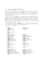
Contents
Disclaimer
iv
1 Overview of OOMMF
1
2 Installation
2.1 Requirements . . . . . . . . . . . . . . . . .
2.2 Basic Installation . . . . . . . . . . . . . . .
2.2.1 Download . . . . . . . . . . . . . . .
2.2.2 Check Your Platform Configuration .
2.2.3 Compiling and Linking . . . . . . . .
2.2.4 Installing . . . . . . . . . . . . . . .
2.2.5 Using OOMMF Software . . . . . . .
2.2.6 Reporting Problems . . . . . . . . .
2.3 Advanced Installation . . . . . . . . . . . . .
2.3.1 Reducing Disk Space Usage . . . . .
2.3.2 Local Customizations . . . . . . . . .
2.3.3 Optimization . . . . . . . . . . . . .
2.3.4 Parallelization . . . . . . . . . . . . .
2.3.5 Managing OOMMF Platform Names
2.4 Platform Specific Installation Issues . . . . .
2.4.1 Unix Configuration . . . . . . . . . .
2.4.2 Microsoft Windows Options . . . . .
2.4.3 Mac OS X Configuration . . . . . . .
.
.
.
.
.
.
.
.
.
.
.
.
.
.
.
.
.
.
.
.
.
.
.
.
.
.
.
.
.
.
.
.
.
.
.
.
.
.
.
.
.
.
.
.
.
.
.
.
.
.
.
.
.
.
.
.
.
.
.
.
.
.
.
.
.
.
.
.
.
.
.
.
.
.
.
.
.
.
.
.
.
.
.
.
.
.
.
.
.
.
.
.
.
.
.
.
.
.
.
.
.
.
.
.
.
.
.
.
.
.
.
.
.
.
.
.
.
.
.
.
.
.
.
.
.
.
.
.
.
.
.
.
.
.
.
.
.
.
.
.
.
.
.
.
.
.
.
.
.
.
.
.
.
.
.
.
.
.
.
.
.
.
.
.
.
.
.
.
.
.
.
.
.
.
.
.
.
.
.
.
.
.
.
.
.
.
.
.
.
.
.
.
.
.
.
.
.
.
.
.
.
.
.
.
.
.
.
.
.
.
.
.
.
.
.
.
.
.
.
.
.
.
.
.
.
.
.
.
.
.
.
.
.
.
.
.
.
.
.
.
.
.
.
.
.
.
.
.
.
.
.
.
.
.
.
.
.
.
.
.
.
.
.
.
.
.
.
.
.
.
.
.
.
.
.
.
.
.
.
.
.
.
.
.
.
.
.
.
.
.
.
.
.
.
.
.
.
.
.
.
.
.
.
.
.
.
.
.
.
.
.
.
.
.
.
.
.
.
.
.
.
.
.
.
3
3
4
4
5
9
9
10
10
10
10
10
11
11
13
15
15
16
20
3 Quick Start: Example OOMMF Session
21
4 OOMMF Architecture Overview
27
5 Command Line Launching
29
6 OOMMF Launcher/Control Interface: mmLaunch
32
7 OOMMF eXtensible Solver
7.1 OOMMF eXtensible Solver Interactive Interface: Oxsii
7.2 OOMMF eXtensible Solver Batch Interface: boxsi . . .
7.3 Standard Oxs Ext Child Classes . . . . . . . . . . . . .
7.3.1 Atlases . . . . . . . . . . . . . . . . . . . . . . .
7.3.2 Meshes . . . . . . . . . . . . . . . . . . . . . . .
7.3.3 Energies . . . . . . . . . . . . . . . . . . . . . .
7.3.4 Evolvers . . . . . . . . . . . . . . . . . . . . . .
7.3.5 Drivers . . . . . . . . . . . . . . . . . . . . . . .
7.3.6 Field Objects . . . . . . . . . . . . . . . . . . .
34
34
39
45
46
52
52
66
77
82
i
.
.
.
.
.
.
.
.
.
.
.
.
.
.
.
.
.
.
.
.
.
.
.
.
.
.
.
.
.
.
.
.
.
.
.
.
.
.
.
.
.
.
.
.
.
.
.
.
.
.
.
.
.
.
.
.
.
.
.
.
.
.
.
.
.
.
.
.
.
.
.
.
.
.
.
.
.
.
.
.
.
.
.
.
.
.
.
.
.
.
.
.
.
.
.
.
.
.
.
.
.
.
.
.
.
.
.
.
7.3.7
MIF Support Classes . . . . . . . . . . . . . . . . . . . . . . . . . . . 101
8 Micromagnetic Problem Editor: mmProbEd
102
9 Micromagnetic Problem File Source: FileSource
105
10 The 2D Micromagnetic Solver
10.1 The 2D Micromagnetic Interactive Solver: mmSolve2D . . .
10.2 OOMMF 2D Micromagnetic Solver Batch System . . . . . .
10.2.1 2D Micromagnetic Solver Batch Interface: batchsolve
10.2.2 2D Micromagnetic Solver Batch Scheduling System .
.
.
.
.
.
.
.
.
.
.
.
.
.
.
.
.
.
.
.
.
.
.
.
.
.
.
.
.
.
.
.
.
.
.
.
.
107
107
114
114
117
11 Data Table Display: mmDataTable
126
12 Data Graph Display: mmGraph
129
13 Vector Field Display: mmDisp
134
14 Data Archive: mmArchive
149
15 Documentation Viewer: mmHelp
151
16 Command Line Utilities
16.1 Bitmap File Format Conversion: any2ppm . . . . . .
16.2 Making Data Tables from Vector Fields: avf2odt . . .
16.3 Vector Field File Format Conversion: avf2ovf . . . . .
16.4 Making Bitmaps from Vector Fields: avf2ppm . . . .
16.5 Making PostScript from Vector Fields: avf2ps . . . .
16.6 Vector Field File Difference: avfdiff . . . . . . . . . .
16.7 Cyclic Redundancy Check: crc32 . . . . . . . . . . .
16.8 Killing OOMMF Processes: killoommf . . . . . . . .
16.9 Launching the OOMMF host server: launchhost . . .
16.10Calculating H Fields from Magnetization: mag2hfield
16.11MIF Format Conversion: mifconvert . . . . . . . . .
16.12ODT Column Extraction: odtcols . . . . . . . . . . .
16.13OOMMF and Process ID Information: pidinfo . . . .
16.14Process Nicknames: nickname . . . . . . . . . . . . .
16.15Platform-Independent Make: pimake . . . . . . . . .
.
.
.
.
.
.
.
.
.
.
.
.
.
.
.
153
153
154
158
160
163
167
167
169
170
171
172
173
174
175
176
.
.
.
.
179
179
179
181
187
17 Problem Specification File Formats (MIF)
17.1 MIF 2.1 . . . . . . . . . . . . . . . . . . .
17.1.1 MIF 2.1 File Overview . . . . . . .
17.1.2 MIF 2.1 Extension Commands . . .
17.1.3 Specify Conventions . . . . . . . .
ii
.
.
.
.
.
.
.
.
.
.
.
.
.
.
.
.
.
.
.
.
.
.
.
.
.
.
.
.
.
.
.
.
.
.
.
.
.
.
.
.
.
.
.
.
.
.
.
.
.
.
.
.
.
.
.
.
.
.
.
.
.
.
.
.
.
.
.
.
.
.
.
.
.
.
.
.
.
.
.
.
.
.
.
.
.
.
.
.
.
.
.
.
.
.
.
.
.
.
.
.
.
.
.
.
.
.
.
.
.
.
.
.
.
.
.
.
.
.
.
.
.
.
.
.
.
.
.
.
.
.
.
.
.
.
.
.
.
.
.
.
.
.
.
.
.
.
.
.
.
.
.
.
.
.
.
.
.
.
.
.
.
.
.
.
.
.
.
.
.
.
.
.
.
.
.
.
.
.
.
.
.
.
.
.
.
.
.
.
.
.
.
.
.
.
.
.
.
.
.
.
.
.
.
.
.
.
.
.
.
.
.
.
.
.
.
.
.
.
.
.
.
.
.
.
.
.
.
.
.
.
.
.
.
.
.
.
.
.
.
.
.
.
.
.
.
.
.
.
.
.
.
.
17.1.4 Variable Substitution . . . . . . . . . . . . . . . . .
17.1.5 Sample MIF 2.1 File . . . . . . . . . . . . . . . . .
17.2 MIF 2.2 . . . . . . . . . . . . . . . . . . . . . . . . . . . .
17.2.1 Differences between MIF 2.2 and MIF 2.1 Formats
17.2.2 MIF 2.2 New Extension Commands . . . . . . . . .
17.2.3 Sample MIF 2.2 File . . . . . . . . . . . . . . . . .
17.3 MIF 1.1 . . . . . . . . . . . . . . . . . . . . . . . . . . . .
17.3.1 Material parameters . . . . . . . . . . . . . . . . .
17.3.2 Demag specification . . . . . . . . . . . . . . . . . .
17.3.3 Part geometry . . . . . . . . . . . . . . . . . . . . .
17.3.4 Initial magnetization . . . . . . . . . . . . . . . . .
17.3.5 Experiment parameters . . . . . . . . . . . . . . . .
17.3.6 Output specification . . . . . . . . . . . . . . . . .
17.3.7 Miscellaneous . . . . . . . . . . . . . . . . . . . . .
17.4 MIF 1.2 . . . . . . . . . . . . . . . . . . . . . . . . . . . .
.
.
.
.
.
.
.
.
.
.
.
.
.
.
.
.
.
.
.
.
.
.
.
.
.
.
.
.
.
.
.
.
.
.
.
.
.
.
.
.
.
.
.
.
.
.
.
.
.
.
.
.
.
.
.
.
.
.
.
.
.
.
.
.
.
.
.
.
.
.
.
.
.
.
.
.
.
.
.
.
.
.
.
.
.
.
.
.
.
.
.
.
.
.
.
.
.
.
.
.
.
.
.
.
.
.
.
.
.
.
.
.
.
.
.
.
.
.
.
.
.
.
.
.
.
.
.
.
.
.
.
.
.
.
.
.
.
.
.
.
.
.
.
.
.
.
.
.
.
.
18 Data Table File Format (ODT)
19 Vector Field File Format (OVF)
19.1 The OVF 1.0 format . . . . . .
19.1.1 Segment Header block .
19.1.2 Data block . . . . . . . .
19.2 The OVF 2.0 format . . . . . .
19.3 The OVF 0.0 format . . . . . .
197
198
201
201
202
204
209
209
211
211
213
213
215
216
218
219
.
.
.
.
.
.
.
.
.
.
.
.
.
.
.
.
.
.
.
.
.
.
.
.
.
.
.
.
.
.
.
.
.
.
.
.
.
.
.
.
.
.
.
.
.
.
.
.
.
.
.
.
.
.
.
.
.
.
.
.
.
.
.
.
.
.
.
.
.
.
.
.
.
.
.
.
.
.
.
.
.
.
.
.
.
.
.
.
.
.
.
.
.
.
.
.
.
.
.
.
.
.
.
.
.
.
.
.
.
.
.
.
.
.
.
.
.
.
.
.
.
.
.
.
.
219
220
221
222
225
227
20 Troubleshooting
230
21 References
234
22 Credits
236
iii
Disclaimer
This software was developed at the National Institute of Standards and Technology by
employees of the Federal Government in the course of their official duties. Pursuant to Title
17, United States Code, Section 105, this software is not subject to copyright protection and
is in the public domain.
OOMMF is an experimental system. NIST assumes no responsibility whatsoever for
its use by other parties, and makes no guarantees, expressed or implied, about its quality,
reliability, or any other characteristic.
We would appreciate acknowledgement if the software is used. When referencing OOMMF
software, we recommend citing the NIST technical report, M. J. Donahue and D. G. Porter,
“OOMMF User’s Guide, Version 1.0,” NISTIR 6376, National Institute of Standards and
Technology, Gaithersburg, MD (Sept 1999).
Commercial equipment and software referred to on these pages are identified for informational purposes only, and does not imply recommendation of or endorsement by the National
Institute of Standards and Technology, nor does it imply that the products so identified are
necessarily the best available for the purpose.
iv
1
Overview of OOMMF
The goal of the OOMMF1 (Object Oriented Micromagnetic Framework) project in the Information Technology Laboratory (ITL) at the National Institute of Standards and Technology
(NIST) is to develop a portable, extensible public domain micromagnetic program and associated tools. This code will form a completely functional micromagnetics package, but will
also have a well documented, flexible programmer’s interface so that people developing new
code can swap their own code in and out as desired. The main contributors to OOMMF are
Mike Donahue and Don Porter.
In order to allow a programmer not familiar with the code as a whole to add modifications
and new functionality, we feel that an object oriented approach is critical, and have settled
on C++ as a good compromise with respect to availability, functionality, and portability.
In order to allow the code to run on a wide variety of systems, we are writing the interface
and glue code in Tcl/Tk. This enables our code to operate across a wide range of Unix
platforms, Windows NT, and Windows 9X.
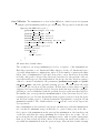
The code may be modified at 3 distinct levels. At the top level, individual programs
interact via well-defined protocols across network sockets. One may connect these modules
together in various ways from the user interface, and new modules speaking the same protocol
can be transparently added. The second level of modification is at the Tcl/Tk script level.
Some modules allow Tcl/Tk scripts to be imported and executed at run time, and the top
level scripts are relatively easy to modify or replace. At the lowest level, the C++ source is
provided and can be modified, although at present the documentation for this is incomplete
(cf. the “OOMMF Programming Manual”).
The first portion of OOMMF released was a magnetization file display program called
mmDisp. A working release2 of the complete OOMMF project was first released in October,
1998. It included a problem editor, a 2D micromagnetic solver, and several display widgets,
including an updated version of mmDisp. The solver can be controlled by an interactive
interface (Sec. 10.1), or through a sophisticated batch control system (Sec. 10.2). This solver
was originally based on a micromagnetic code that Mike Donahue and Bob McMichael
had previously developed. It utilizes a Landau-Lifshitz ODE solver to relax 3D spins on
a 2D mesh of square cells, using FFT’s to compute the self-magnetostatic (demag) field.
Anisotropy, applied field, and initial magnetization can be varied pointwise, and arbitrarily
shaped elements can be modeled.
The current development version, OOMMF 1.2, includes Oxs, the OOMMF eXtensible
Solver. Oxs offers users of OOMMF the ability to extend Oxs with their own modules. The
details of programming an Oxs extension module are found in the OOMMF Programming
Manual 3 . The extensible nature of the Oxs solver means that its capabilities may be varied
as necessary for the problem to be solved. Oxs modules distributed as part of OOMMF
support full 3D simulations suitable for modeling layered materials.
1
http://math.nist.gov/oommf/
http://math.nist.gov/oommf/software.html
3
http://math.nist.gov/oommf/doc/
2
1
If you want to receive e-mail notification of updates to this project, register your e-mail
address with the “µMAG Announcement” mailing list:
http://www.ctcms.nist.gov/˜rdm/email-list.html.
The OOMMF developers are always interested in your comments about OOMMF. See the
Credits (Sec. 22) for instructions on how to contact them, and for information on referencing
OOMMF.
2
2
Installation
2.1
Requirements
OOMMF software is written in C++ and Tcl. It uses the Tcl-based Tk Windowing Toolkit
to create graphical user interfaces that are portable to many varieties of Unix as well as
Microsoft Windows.
Tcl and Tk must be installed before installing OOMMF. Tcl and Tk are available for
free from the Tcl Developer Xchange4 . We recommend the latest stable versions of Tcl and
Tk concurrent with this release of OOMMF. OOMMF requires at least Tcl version 7.5 and
Tk version 4.1 on Unix platforms, and requires at least Tcl version 8.0 and Tk version 8.0
on Microsoft Windows platforms. OOMMF software does not support any alpha or beta
versions of Tcl/Tk, and each release of OOMMF may not work with later releases of Tcl/Tk.
Check the release dates of both OOMMF and Tcl/Tk to ensure compatibility.
A Tcl/Tk installation includes two shell programs. The names of these programs may
vary depending on the Tcl/Tk version and the type of platform. The first shell program
contains an interpreter for the base Tcl language. In the OOMMF documentation we refer
to this program as tclsh. The second shell program contains an interpreter for the base
Tcl language extended by the Tcl commands supplied by the Tk toolkit. In the OOMMF
documentation we refer to this program as wish. Consult your Tcl/Tk documentation to
determine the actual names of these programs on your platform (for example, tclsh83.exe
or wish8.0).
OOMMF applications communicate via TCP/IP network sockets. This means that
OOMMF requires support for networking, even on a stand-alone machine. At a minimum,
OOMMF must be able to access the loopback interface so that the host can talk to itself
using TCP/IP.
OOMMF applications that use Tk require a windowing system and a valid display. On
Unix systems, this means that an X server must be running. If you need to run OOMMF
applications on a Unix system without display hardware or software, you may need to start
the application with command line option -tk 0 (see Sec. 5) or use the Xvfb5 virtual frame
buffer.
The OOMMF source distribution unpacks into a directory tree containing about 800
files and directories, occupying approximately 10 MB of storage. The amount of disk space
needed for compiling and linking varies greatly between platforms; allow an additional 15 MB
to 80 MB for the build. Removing intermediate object modules (cf. the pimake “objclean”
target, in Reducing Disk Space Usage, Sec. 2.3.1, below ) reduces the final space requirement
for source + binary executables to between 15 MB and 25 MB. The OOMMF distribution
containing Windows executables unpacks into a directory tree occupying about 15 MB of
storage. Note: On a non-compressed FAT16 file system on a large disk, OOMMF may
take up much more disk space. This is because on such systems, the minimum size of any
4
5
http://purl.org/tcl/home/
http://www.itworld.com/AppDev/1461/UIR000330xvfb/
3
file is large, as much as 32 KB. Since this is much larger than many files in the OOMMF
distribution require, a great deal of disk space is wasted.
To build OOMMF software from source code, you will need a C++ compiler capable
of handling C++ templates, C++ exceptions, and (for the OOMMF eXtensible Solver) the
C++ Standard Template Library. You will need other software development utilities for your
platform as well. We do development and test builds on the following platforms, although
porting to others should not be difficult:
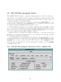
Platform
Windows
Compilers
Microsoft Visual C++, Borland C++,
Intel C++, MinGW g++
Linux/x86
Gnu g++, Intel C++, Portland Group pgCC
Linux/Itanium
Intel C++, Gnu g++
Mac OS X
Gnu g++
MIPS/IRIX 6 (SGI) MIPSpro C++, Gnu g++
SPARC/Solaris
Sun Workshop C++, Gnu g++
System Notes:
• Linux/x86: Both 32-bit x86 and 64-bit x86 64 supported.
• Windows: Microsoft Visual C++ compiler 6.0 or later required.
2.2
Basic Installation
Follow the instructions in the following sections, in order, to prepare OOMMF software for
use on your computer.
2.2.1
Download
The latest release of the OOMMF software may be retrieved from the OOMMF download
page6 . Each release is available in two formats. The first format is a gzipped tar file containing an archive of all the OOMMF source code. The second format is a .zip compressed
archive containing source code and pre-compiled executables for Microsoft Windows. Each
Windows binary distribution is compatible with only a particular sequence of releases of
Tcl/Tk. For example, a Windows binary release for Tcl/Tk 8.3.x is compatible with Tcl/Tk
8.3.0, 8.3.1, . . . . Other release formats, e.g., pre-compiled executables for Microsoft Windows NT running on a Compaq Alpha Systems RISC-based microprocessor system, and/or
compatible with older versions of Tcl/Tk, may be made available upon request.
For the first format, unpack the distribution archive using gunzip and tar:
gunzip -c oommf12a4_20040908.tar.gz | tar xvf 6
http://math.nist.gov/oommf/software.html
4
For the other format(s), you will need a utility program to unpack the .zip archive.
This program must preserve the directory structure of the files in the archive, and it must
be able to generate files with names not limited to the old MSDOS 8.3 format. Some very
old versions of the pkzip utility do not have these properties. One utility program which is
known to work is UnZip7 .
Using your utility, unpack the .zip archive, e.g.
unzip oommf12a4_20040908_84.zip
For either distribution format, the unpacking sequence creates a subdirectory oommf
which contains all the files and directories of the OOMMF distribution. If a subdirectory
named oommf already existed (say, from an earlier OOMMF release), then files in the new
distribution overwrite those of the same name already on the disk. Some care may be needed
in that circumstance to be sure that the resulting mix of files from an old and a new OOMMF
distribution combine to create a working set of files.
2.2.2
Check Your Platform Configuration
After downloading and unpacking the OOMMF software distribution, all the OOMMF software is contained in a subdirectory named oommf. Start a command line interface (a shell
on Unix, or the MS-DOS Prompt on Microsoft Windows), and change the working directory to the directory oommf. Find the Tcl shell program installed as part of your Tcl/Tk
installation. In this manual we call the Tcl shell program tclsh, but the actual name of the
executable depends on the release of Tcl/Tk and your platform type. Consult your Tcl/Tk
documentation.
In the root directory of the OOMMF distribution is a file named oommf.tcl. It is the
bootstrap application (Sec. 5) which is used to launch all OOMMF software. With the
command line argument +platform, it will print a summary of your platform configuration
when it is evaluated by tclsh. This summary describes your platform type, your C++
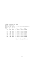
compiler, and your Tcl/Tk installation. As an example, here is the typical output on a
Linux/x86 64 system:
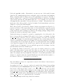
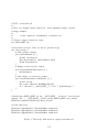
$ tclsh8.4 oommf.tcl +platform
oommf.tcl 1.2.0.4 info:
OOMMF release 1.2.0.4
Platform Name:
linux-x86_64
Tcl name for OS:
Linux 2.6.18-274.7.1.el5
C++ compiler:
/usr/bin/g++
Version string:
g++ (GCC) 4.1.2 20080704 (Red Hat 4.1.2-51)
Shell details --tclsh (running):
/usr/bin/tclsh8.4
--> Version 8.4.13, 64 bit, threaded
7
http://www.info-zip.org/pub/infozip/UnZip.html
5
tclsh (OOMMF):
/usr/bin/tclsh8.4
--> Version 8.4.13, 64 bit, threaded
filtersh:
/usr/local/oommf/app/omfsh/linux-x86_64/filtersh
--> Version 8.4.13, 64 bit, threaded
tclConfig.sh:
/usr/lib64/tclConfig.sh
--> Version 8.4.13
wish (OOMMF):
/usr/bin/wish8.4
--> Version 8.4.13, Tk 8.4.13, 64 bit, threaded
tkConfig.sh:
/usr/lib64/tkConfig.sh
--> Tk Version 8.4.13
OOMMF threads:
Yes
Default thread count:
4
NUMA support:
No
Temp file directory:
/tmp
If oommf.tcl +platform doesn’t print a summary similar to the above, it should instead print an error message describing why it can’t. For example, if your Tcl installation is
older than release 7.5, the error message will report that fact. Follow the instructions provided and repeat until oommf.tcl +platform successfully prints a summary of the platform
configuration information.
The first line of the example summary reports that OOMMF recognizes the platform by
the name linux-x86 64. OOMMF software recognizes many of the more popular computing
platforms, and assigns each a platform name. The platform name is used by OOMMF in
index and configuration files and to name directories so that a single OOMMF installation
can support multiple platform types. If oommf.tcl +platform reports the platform name
to be “unknown”, then you will need to add some configuration files to help OOMMF assign
a name to your platform type, and associate with that name some of the key features of your
computer. See the section on “Managing OOMMF platform names” (Sec. 2.3.5) for further
instructions.
The second line reports the operating system version, which is mainly useful to OOMMF
developers when fielding bug reports. The third line reports what C++ compiler will be
used to build OOMMF from its C++ source code. If you downloaded an OOMMF release
with pre-compiled binaries for your platform, you may ignore this line. Otherwise, if this line
reports “none selected”, or if it reports a compiler other than the one you wish to use, then
you will need to tell OOMMF what compiler to use. To do that, you must edit the appropriate configuration file for your platform. Continuing the example above, one would edit the
file config/platforms/linux-x86 64.tcl. Editing instructions are contained within the
file. On other platforms the name linux-x86 64 in config/platforms/linux-x86 64.tcl
should be replaced with the platform name OOMMF reports for your platform. For example,
on a 32-bit Windows machine using an x86 processor, the corresponding configuration file is
config/platforms/wintel.tcl.
The next group of lines describe the Tcl configuration OOMMF finds on your platform.
The first couple of lines, “tclsh (running)”, describe the Tcl shell running the oommf.tcl
6
script. After that, the “tclsh (OOMMF)” subgroup describes the Tcl shell that OOMMF
will launch when it needs to run vanilla Tcl scripts. If the OOMMF binaries have been built,
then there will also be a filtersh subgroup, which describes the augmented Tcl shell used
to run many of the OOMMF support scripts. All of these shells should report the same
version, bitness, and threading information. If OOMMF can’t find tclsh, or if it finds the
wrong one, you can correct this by setting the environment variable OOMMF TCLSH to
the absolute location of tclsh. (For information about setting environment variables, see
your operating system documentation.)
Following the Tcl shell information, the tclConfig.sh lines report the name of the
configuration file installed as part of Tcl, if any. Conventional Tcl installations on Unix
systems and within the Cygwin environment on Windows have such a file, usually named
tclConfig.sh. The Tcl configuration file records details about how Tcl was built and where
it was installed. On Windows platforms, this information is recorded in the Windows registry, so it is normal to have oommf.tcl +platform report “none found”. If oommf.tcl
+platform reports “none found”, but you know that an appropriate Tcl configuration file is
present on your system, you can tell OOMMF where to find the file by setting the environment variable OOMMF TCL CONFIG to its absolute filename. In unusual circumstances,
OOMMF may find a Tcl configuration file which doesn’t correctly describe your Tcl installation. In that case, use the environment variable OOMMF TCL CONFIG to instruct
OOMMF to use a different file that you specify, and, if necessary, edit that file to include a
correct description of your Tcl installation.
Next, the oommf.tcl +platform reports similar information about the wish and Tk
configuration. The environment variables OOMMF TK CONFIG and OOMMF WISH may be used to
tell OOMMF where to find the Tk configuration file and the wish program, respectively.
Following the Tk information are some lines reporting “thread” build and run status.
Threads are used by OOMMF to implement parallelism in the Oxs (oxsii and boxsi) 3D
solvers on multi-processor/multi-core shared memory machines. In order to build or run
a parallel version of OOMMF, you must have a thread-enabled version of Tcl. The Tcl
thread status is indicated on the first thread status line. If Tcl is thread enabled, then
the default OOMMF build process will create a threaded version of OOMMF. You can
override this behavior if you wish to build a non-parallel version of OOMMF by editing the
oommf threads value in the config/platforms/ file for your platform.
If Tcl and OOMMF threads are enabled, then the next line will show the default number
of threads run by the Oxs solvers. (This value may vary between machines, depending on
the number of processors in the machine.) You can change this by setting the thread count
value in the config/platforms/ file for your platform. The default can be overridden at
run time by the environment variable OOMMF THREADS, or by the oxsii/boxsi command
line option -threads. If NUMA support is possible on your platform (see “Parallelization,”
Sec. 2.3.4 below), then the next line of thread info will indicate whether or not the build
process will create NUMA-aware Oxs solvers.
After the thread info, oommf.tcl +platform reports the directory that OOMMF will
use to write temporary files. This directory is used, for example, to transfer magnetization
7
data from the micromagnetic solvers to the mmDisp display module. You must have write
access to this directory. If you don’t like the OOMMF default, you may change it via the
path directory temporary setting in the config/platforms/ file for your platform. Or
you can set the environment variable OOMMF TEMP, which will override all other settings.
If any environment variables relevant to OOMMF are set, then oommf.tcl +platform
will report these next, followed finally by any warnings about possible problems with your
Tcl/Tk installation, such as if you are missing important header files.
If oommf.tcl +platform indicates problems with your Tcl/Tk installation, it may be
easiest to re-install Tcl/Tk taking care to perform a conventional installation. OOMMF
deals best with conventional Tcl/Tk installations. If you do not have the power to re-install
an existing broken Tcl/Tk installation (perhaps you are not the sysadmin of your machine),
you might still install your own copy of Tcl/Tk in your own user space. In that case, if your
private Tcl/Tk installation makes use of shared libraries, take care that you do whatever is
necessary on your platform to be sure that your private tclsh and wish find and use your
private shared libraries instead of those from the system Tcl/Tk installation. This might
involve setting an environment variable (such as LD LIBRARY PATH). If you use a private
Tcl/Tk installation, you also want to be sure that there are no environment variables like
TCL LIBRARY or TK LIBRARY that still refer to the system Tcl/Tk installation.
Additional Configuration Issues on Windows A few other configurations should be
checked on Windows platforms. First, note that absolute filenames on Windows makes use
of the backslash (\) to separate directory names. On Unix and within Tcl the forward slash
(/) is used to separate directory names in an absolute filename. In this manual we usually
use the Tcl convention of forward slash as separator. In portions of the manual pertaining
only to MS Windows we use the backslash as separator. There may be instructions in this
manual which do not work exactly as written on Windows platforms. You may need to
replace forward slashes with backward slashes in pathnames when working on Windows.
OOMMF software needs networking support that recognizes the host name localhost.
It may be necessary to edit a file which records that localhost is a synonym for the loopback interface (127.0.0.1). If a file named hosts exists in your system area (for example,
C:\Windows\hosts), be sure it includes an entry mapping 127.0.0.1 to localhost. If no
hosts file exists, but a hosts.sam file exists, make a copy of hosts.sam with the name
hosts, and edit the copy to have the localhost entry.
The directory that holds the tclsh and wish programs also holds several *.dll files that
OOMMF software needs to find to run properly. Normally when the OOMMF bootstrap
application (Sec. 5) or mmLaunch (Sec. 6) is used to launch OOMMF programs, they take
care of making sure the necessary *.dll files can be found. As an additional measure, you
might want to add the directory which holds the tclsh and wish programs to the list of
directories stored in the PATH environment variable. All the directories in the PATH are
searched for *.dll files needed when starting an executable.
8
2.2.3
Compiling and Linking
If you downloaded a distribution with pre-compiled executables, you may skip this section.
When building OOMMF software from source code, be sure the C++ compiler reported
by oommf.tcl +platform is properly configured. In particular, if you are running on a Windows system, please read carefully the notes in Advanced Installation, Sec. 2.4.2, pertaining
to your compiler.
The compiling and linking of the C++ portions of OOMMF software are guided by the
application pimake (Sec. 16.15) (“Platform Independent Make”) which is distributed as part
of the OOMMF release. To begin building OOMMF software with pimake, first change your
working directory to the root directory of the OOMMF distribution:
cd .../path/to/oommf
If you unpacked the new OOMMF release into a directory oommf which contained an
earlier OOMMF release, use pimake to build the target upgrade to clear away any source
code files which were in a former distribution but are not part of the latest distribution:
tclsh oommf.tcl pimake upgrade
Next, build the target distclean to clear away any old executables and object files which
are left behind from the compilation of the previous distribution:
tclsh oommf.tcl pimake distclean
Next, to build all the OOMMF software, run pimake without specifying a target:
tclsh oommf.tcl pimake
On some platforms, you cannot successfully compile OOMMF software if there are OOMMF
programs running. Check that all OOMMF programs have terminated (including those in
the background) before trying to compile and link OOMMF.
When pimake calls on a compiler or other software development utility, the command line
is printed, so that you may monitor the build process. Assuming a proper configuration for
your platform, pimake should be able to compile and link all the OOMMF software without
error. If pimake reports errors, please first consult Troubleshooting (Sec. 20) to see if a fix
is already documented. If not, please send both the complete output from pimake and the
output from oommf.tcl +platform to the OOMMF developers when you e-mail to ask for
help.
2.2.4
Installing
The current OOMMF release does not support an installation procedure. For now, simply
run the executables from the directories in which they were unpacked/built.
9
2.2.5
Using OOMMF Software
To start using OOMMF software, run the OOMMF bootstrap application (Sec. 5). This
may be launched from the command line interface:
tclsh oommf.tcl
If you prefer, you may launch the OOMMF bootstrap application oommf.tcl using whatever graphical “point and click” interface your operating system provides. By default, the
OOMMF bootstrap application will start up a copy of the OOMMF application mmLaunch
(Sec. 6) in a new window.
If you publish material created with the aid of OOMMF, please refer to Credits (Sec. 22)
for citation information.
2.2.6
Reporting Problems
If you encounter problems when installing or using OOMMF, please report them to the
OOMMF developers. The oommf.tcl +platform command has been designed in large part
to help OOMMF developers debug installation problems, so PLEASE be sure to include
the complete output from oommf.tcl +platform in your report. See also the section on
troubleshooting (Sec. 20) for additional instructions.
2.3
Advanced Installation
The following sections provide instructions for some additional installation options.
2.3.1
Reducing Disk Space Usage
To delete the intermediate files created when building the OOMMF software from source
code, use pimake (Sec. 16.15) to build the target objclean in the root directory of the
OOMMF distribution.
tclsh oommf.tcl pimake objclean
Running your platform strip utility on the OOMMF executable files should also reduce
their size somewhat.
2.3.2
Local Customizations
OOMMF software supports local customization of some of its features. All OOMMF programs load the file config/options.tcl, which contains customization commands as well
as editing instructions. As it is distributed, config/options.tcl directs programs to also
load the file config/local/options.tcl, if it exists. Because future OOMMF releases
may overwrite the file config/options.tcl, permanent customizations should be made by
copying config/options.tcl to config/local/options.tcl and editing the copy. It is
10
recommended that you leave in the file config/local/options.tcl only the customization
commands necessary to change those options you wish to modify. Remove all other options so that overwrites by subsequent OOMMF releases are allowed to change the default
behavior.
Notable available customizations include the choice of which network port the host service
directory application (Sec. 4) uses, and the choice of what program is used for the display of
help documentation. By default, OOMMF software uses the application mmHelp (Sec. 15),
which is included in the OOMMF release, but the help documentation files are standard
HTML, so any web browser (for example, Netscape Navigator or Microsoft Internet Explorer)
may be used instead. Complete instructions are in the file config/options.tcl.
2.3.3
Optimization
In the interest of successful compilation of a usable software package “out of the box,” the
default configuration for OOMMF does not attempt to achieve much in terms of optimization.
However, in each platform’s configuration file (for example, config/platforms/wintel.tcl),
there are alternative values for the configuration’s optimization flags, available as comments.
If you are familiar with your compiler’s command line options, you may experiment with
other choices as well. You can edit the platform configuration file to replace the default
selection with another choice that provides better computing performance. For example, in
config/platforms/wintel.tcl, alternative optimization flags for the MSVC++ compiler
are defined with the line:
$config SetValue program_compiler_c++_option_opt {format "/G5 /Ox"}
The extensible solver, Oxs, can be compiled with debugging support for extensive runtime code checks. This will significantly reduce computation performance. In the standard
OOMMF distributions, these checks should be disabled. You may verify this by checking
that the following line appears in the file config/options.tcl:
Oc_Option Add * Platform cflags {-def NDEBUG}
To enable these checks, either comment/remove this line, or else add to the config/local/options.tcl
file a “cflags” option line without “-def NDEBUG”, such as
Oc_Option Add * Platform cflags {-warn 1}
The config/local/options.tcl file may be created if it does not already exist.
2.3.4
Parallelization
The OOMMF Oxs 3D solvers (oxsii amd boxsi) can be built thread-enabled to allow
parallel processing on multi-processor/multi-core machines. In order to build and run a
parallel version of OOMMF, you must have a thread-enabled version of Tcl. Most standard
binary releases of Tcl today are thread-enabled, so OOMMF releases that include pre-built
11
executables are built thread-enabled. If you build OOMMF from source, then by default
OOMMF will be built thread-enabled if your Tcl is thread-enabled. As explained earlier,
you can check thread build status with the tclsh oommf.tcl +platform command. If you
want to force a non-threaded build of OOMMF, then edit the config/platforms/ file for
your platform. In the section labeled LOCAL CONFIGURATION, you will find a line that looks
like
# $config SetValue oommf_threads 0
Uncomment this line (i.e., remove the leading ‘#’ character) to force a non-threaded build.
Then run
tclsh oommf.tcl pimake distclean
tclsh oommf.tcl pimake
from the OOMMF root directory to create a fresh build.
You can use the tclsh oommf.tcl +platform command to see the default number of
compute threads that will be run by the Oxs 3D solver programs oxsii and boxsi. You
can modify the default by editing the oommf thread count value in the config/platforms/
file for your platform. You can override the default at run time by setting the environment
variable OOMMF THREADS, or by using the command line option -threads to oxsii and boxsi.
Some multi-processor machines have a non-uniform memory architecture (NUMA), which
means that although each processor can access all of system memory, some parts of memory
can be accessed faster than others. Typically this is accomplished by dividing the system
memory and processors into “nodes.” Memory accesses within a node are faster than accesses
between nodes, and depending on the architecture access latency and bandwidth may be
different between different node pairs. Examples of machines with NUMA include some
multi-processor AMD Opteron and Intel Nehalem Xeon boxes.
Computer programs such as OOMMF can run on NUMA machines without making any
special allowances for the memory architecture. However, a program that is written to take
advantage of the faster local (intra-node) memory accesses can sometimes run significantly
faster. OOMMF contains NUMA-aware code, but this code is highly operating system specific. At present, OOMMF can be built with NUMA support only on Linux (32- and 64-bit)
systems. To do this, you must install the operating system NUMA support packages “numactl” and “numactl-devel”. The names may vary somewhat between Linux distributions,
but the first typically includes the executable numactl and the second includes the header
file numa.h. Once the numactl package is installed, you can run the command
numactl --hardware
to get an overview of the memory architecture on your machine. If this shows you have only
one node, then there is no advantage to making a NUMA-aware build of OOMMF.
The next step is to edit the config/platforms for your platform. For example, on a
64-bit Linux box this file is config/platforms/linux-x86 64.tcl. In the section labeled
LOCAL CONFIGURATION, find the line
12
# $config SetValue use_numa 1
Edit this to remove the leading ‘#’ character. Alternatively (and, actually, preferably), create
a local subdirectory and make a local configuration file with the same platform name; e.g.,
config/platforms/local/linux-x86 64.tcl on a 64-bit Linux machine. Add the line
$config SetValue use_numa 1
to this file. (The advantage of using a config/platforms/local file is that you can make
changes without modifying the original OOMMF source code, which makes it easier to port
your local changes to future releases of OOMMF.) If this is done correctly, then the command
‘tclsh oommf.tcl +platform’ will show that NUMA support is enabled. Then simply run
‘tclsh oommf.tcl pimake distclean’ and ‘tclsh oommf.tcl pimake’ from the OOMMF
root directory to build a NUMA-aware version of OOMMF.
To activate the NUMA-aware code, you must specify the -numanodes option on the
oxsii/boxsi command line, or set the the environment variable OOMMF NUMANODES. Check
the Oxs documentation (Sec. 7) for details.
2.3.5
Managing OOMMF Platform Names
OOMMF software classifies computing platforms into different types using the scripts in the
directory config/names relative to the root directory of the OOMMF distribution. Each
type of computing platform is assigned a unique name. These names are used as directory
names and in index and configuration files so that a single OOMMF installation may contain
platform-dependent sections for many different types of computing platforms.
To learn what name OOMMF software uses to refer to your computing platform, run
tclsh oommf.tcl +platform
in the OOMMF root directory.
Changing the name OOMMF assigns to your platform First, use pimake (Sec. 16.15)
to build the target distclean to clear away any compiled executables built using the old
platform name.
tclsh oommf.tcl pimake distclean
Then, to change the name OOMMF software uses to describe your platform from foo to
bar, simply rename the file
config/names/foo.tcl
to
config/names/bar.tcl
and
config/platforms/foo.tcl
to
config/platforms/bar.tcl.
After renaming your platform type, you should recompile your executables using the new
platform name.
13
Adding a new platform type If oommf.tcl +platform reports the platform name
unknown, then none of the scripts in config/names/ recognizes your platform type. As
an example, to add the platform name foo to OOMMF’s vocabulary of platform names,
create the file config/names/foo.tcl. The simplest way to proceed is to copy an existing
file in the directory config/names and edit it to recognize your platform.
The files in config/names include Tcl code like this:
Oc_Config New _ \
[string tolower [file rootname [file tail [info script]]]] {
# In this block place the body of a Tcl proc which returns 1
# if the machine on which the proc is executed is of the
# platform type identified by this file, and which returns 0
# otherwise.
#
# The usual Tcl language mechanism for discovering details
# about the machine on which the proc is running is to
# consult the global Tcl variable ’tcl_platform’. See the
# existing files for examples, or contact the OOMMF
# developers for further assistance.
}
After creating the new platform name file config/names/foo.tcl, you also need to
create a new platform file config/platforms/foo.tcl. A reasonable starting point is to
copy the file config/platforms/unknown.tcl for editing. Contact the OOMMF developers
for assistance.
Please consider contributing your new platform recognition and configuration files to the
OOMMF developers for inclusion in future releases of OOMMF software.
Resolving platform name conflicts If the script oommf.tcl +platform reports “Multiple platform names are compatible with your computer”, then there are multiple files in the
directory config/names/ that return 1 when run on your computer. For each compatible
platform name reported, edit the corresponding file in config/names/ so that only one of
them returns 1. Experimenting using tclsh to probe the Tcl variable tcl platform should
assist you in this task. If that fails, you can explicitly assign a platform type corresponding
to your computing platform by matching its hostname. For example, if your machine’s host
name is foo.bar.net:
Oc_Config New _ \
[string tolower [file rootname [file tail [info script]]]] {
if {[string match foo.bar.net [info hostname]]} {
return 1
}
# Continue with other tests...
}
14
Contact the OOMMF developers if you need further assistance.
2.4
Platform Specific Installation Issues
The installation procedure discussed in the previous sections applies to all platforms (Unix,
Windows, Mac OS X). There are, however, some details which pertain only to a particular
platform. These issues are discussed below.
2.4.1
Unix Configuration
Missing Tcl/Tk files The basic installation procedure should be sufficient to install
OOMMF on most Unix systems. Sometimes, however, the build will fail due to missing
Tcl header files (tcl.h, tk.h) or libraries (e.g., libtcl.so, libtk.so). This problem can
usually be solved by installing a “development” version of Tcl/Tk, which may be found on
the operating system installation disks, or may be available from the system vender. There
are also binary releases of Tcl/Tk for a number of systems available from ActiveState, under
the name ActiveTcl8 . Alternatively, one may download the sources for Tcl and Tk from
the Tcl Developer Xchange9 , and build and install Tcl/Tk from source. The Tcl/Tk build
follows the usual Unix configure, make, make install build convention.
Compiler Optimization Options On most systems, OOMMF builds by default with
relatively unaggressive compiler optimization options. As discussed earlier (“Optimiation,”
Sec. 2.3.3)), you may edit the appropriate oommf/config/platforms/ file to change the
default compilation options. However, on some common systems (e.g., Linux, some BSD
variants) OOMMF will try to deduce the hardware architecture (i.e., the CPU subtype,
such as Pentium 3 vs. Pentium 4) and apply architecture-specific options to the compile
commands. This is probably what you want if OOMMF is to be run only on the system on
which it was built, or if it is run on a homogeneous cluster. If, instead, you intend to run
OOMMF on a heterogeneous cluster you may need to restrict the compiler options to those
supported across your target machines. In that case, open the appropriate configuration file
in the oommf/config/platforms/ directory, and look for the lines
# You can override the GuessCPU results by directly setting or
# unsetting the cpuopts variable, e.g.,
#
#
set cpuopts [list -march=athlon]
# or
#
unset cpuopts
#
8
9
http://www.activestate.com/Products/ActiveTcl/
http://purl.org/tcl/home/
15
Uncomment either the “unset cpuopts” line to make a generic build, or else edit the “set
cpuopts” line to an appropriate common-denominator architecture and uncomment that line.
In a similar vein, some compilers support a “-fast” switch, which usually creates an
architecture-specific executable. The same considerations apply in this case.
An advanced alternative would be to define separate OOMMF “platforms” for each CPU
subtype in your cluster. At a minimum, this would involve creating separate platform name
files in oommf/config/names/ for each subtype, and then making copies of the appropriate
oommf/config/platforms file for each new platform. The platform name files would have
to be written so as to reliably detect the CPU subtype on each machine. See “Managing
OOMMF platform names” (Sec. 2.3.5) for details on creating platform name files.
2.4.2
Microsoft Windows Options
This section lists installation options for Microsoft Windows.
Using Microsoft Visual C++ If you are building OOMMF software from source using the Microsoft Visual C++ command line compiler, cl.exe, it is necessary to run
vcvars32.bat to set up the path and some environment variables. This file is distributed
as part of Visual C++. You may want to set up your system so this batch file gets run
automatically when you boot the system, or open a command prompt. See your compiler
and system documentation for details.
Using the Cygwin toolkit The Cygwin Project10 is a free port of the GNU development
environment to Windows, which includes the GNU C++ compiler g++. OOMMF has
been successfully built and tested within the Cygwin environment; sample configuration
files config/names/cygtel.tcl and config/platforms/cygtel.tcl are included in the
OOMMF distribution. IMPORTANT: Use a standard Windows build of Tcl/Tk (e.g., the
ActiveTcl release11 ) when configuring, building, and launching OOMMF software. As of this
writing (Oct. 2004), the tclsh distributed with Cygwin (i.e., /usr/bin/tclsh) has problems
involving sockets that make it unsuitable for use with OOMMF. Unfortunately, standard
Windows versions of Tcl are not acquainted with the Cygwin POSIX-style pathnames, so in
many cases you will have to use Windows-style pathnames instead.
Note that OOMMF software determines whether it is running under Cygwin by examining the environment variables OSTYPE and TERM. If either is set to a value beginning
with cygwin, the Cygwin environment is assumed. If you are using the Cygwin environment with different values for both OSTYPE and TERM, you will have to modify the
config/names/cygtel.tcl file accordingly.
10
11
http://www.cygwin.com/
http://www.activestate.com/Products/ActiveTcl/
16
Using Borland C++ OOMMF has been successfully built and tested using the Borland
C++ command line compiler version 5.5. However, a couple preparatory steps are necessary
before building OOMMF with this compiler.
1. Properly complete bcc55 compiler installation.
Be sure to read the readme.txt file in the BCC55 subdirectory of the Borland install
directory. In particular, check that the bcc32.cfg and ilink32.cfg configuration files
exist in the BIN subdirectory, and have appropriate contents. If you omit this step you
will get error messages during the OOMMF build process relating to the inability of
the Borland compiler to find system header files and libraries. You will probably also
need to add the Borland BIN directory to your PATH environment variable. Some of the
Borland tools are fragile with respect to spaces in their pathnames, so you should either
select the Borland install directory to be one without spaces anywhere in the pathname
(e.g., use C:\Borland\ instead of "C:\Program Files\Borland\"), or at least when
setting the PATH use the “8dot3” style short name version of each component of the
Borland install directory, e.g.,
PATH=C:\Progra~1\Borland\BCC55\Bin;%PATH%
Use “dir /x” to display both the short and long versions of filenames. The Borland
Developer Studio 2006 install automatically sets the path to include the long name
version of the Borland BIN directory; you should manually change this via the System
dialog box from the Control Panel. Select the Advanced tab, and pull up the Environment Variables sub-dialog. Edit the Path variable as discussed above; check both the
“User variables” and the “System variables” settings. You will need to launch a new
shell (command prompt) for the changes to take effect.
2. Create Borland compatible Tcl and Tk libraries.
The import libraries distributed with Tcl/Tk, release 8.0.3 and later, are not compatible with the Borland C++ linker. However, the command line utility coff2omf,
which is distributed with the Borland compiler, can be used to create suitable libraries
from the Tcl/Tk .lib’s. In the Tcl/Tk library directory (typically C:\Tcl\lib or
"C:\Program Files\Tcl\lib"), issue the following commands
coff2omf tcl84.lib tcl84bc.lib
coff2omf tk84.lib tk84bc.lib
Here tcl84.lib and tk84.lib are the input libraries (in COFF format) and tcl84bc.lib
and tk84bc.lib are the new libraries (in OMF format).
If coff2omf doesn’t work, you can try creating the necessary import libraries directly
from the Tcl/Tk DLL’s. From the Tcl/Tk library directory issue the following commands:
17
impdef -a tcl84bc.def ..\bin\tcl84.dll
implib tcl84bc.lib tcl84bc.def
This creates the Borland compatible import library tcl84bc.lib. Repeat with “tk”
in place of “tcl” to create tk84bc.lib. The “-a” switch requests impdef to add a
leading underscore to function names. This is sufficient for the DLL’s shipped with
Tcl/Tk 8.4, but other releases may require additional tweaking. The module definition
file output by impdef, e.g., tcl84bc.def above, is a plain text file. You may need to
edit this file to add or modify entries.
3. Edit oommf\config\platforms\wintel.tcl
At a minimum, you will have to change the program compiler c++ value to point to
the Borland C++ compiler. The sample wintel.tcl file assumes the librarian tlib
and the linker ilink32 are in the execution path, and that the Borland compatible
import libraries, with names as specified above, are in the Tcl/Tk library directory. If
this is not the case then you will have to make appropriate modifications. Also, you
may need to add the “-o” switch to the linker command to force ordinal usage of the
Borland compatible Tcl/Tk libraries produced in the previous step.
After this, continue with the instructions in Sec. 2.2.3, Compiling and Linking.
Using Digital Mars C++ The Digital Mars12 C++ command line compilers (dmc)
versions 8.50 and earlier do not successfully build this release of OOMMF. The following
notes may help build OOMMF with a later release of dmc.
1. Install the Digital Mars C++ compiler, tools, and STL.
Unpack the dmc archive into a convenient location. The default name for the root
directory of the dmc installation area is “dm”. Unpack the STLport (C++ Standard
Library) into the dmc installation area. The top-level directory in the STLport archive
is “dm”, so if you unzip this archive from the parent directory to the dmc installation
area it will naturally unpack into its standard location. Then modify the dmc configuration to include the STL header files. The dm\bin\sc.ini file should be edited so
that the first element of the INCLUDE path is "%@P%\..\stlport\stlport";
Next, use “set INCLUDE” and “set LIBRARY” from the DOS command prompt to
check that these environment variables are either not set, or else set to values as
needed by the Digital Mars compiler. (These variables names may be used by other
applications, which will conflict with values expected by dmc.) To unset these variables, use the commands “set INCLUDE=” and “set LIBRARY=”. For convenience, you
probably also want to put the dm\bin directory into your environment PATH variable.
12
http://www.digitalmars.com/
18
2. Create compatible Tcl/Tk import libraries.
The Digital Mars linker uses the same library format as the Borland linker, and as in
that case, you will have to build compatible import libraries for the Tcl/Tk libraries.
The free download from Digital Mars does not include a utility to create these import
libraries. If you have purchased the compiler from Digital Mars, you can use the coff2off
or implib tools for this. See the documentation for details. Another option is to use
the Borland tools. See the section above on using Borland C++ for details.
3. Edit oommf\config\platforms\wintel.tcl.
You will need to uncomment the entry for the dmc compiler, and comment out the
other compiler selections. (The comment character is ’#’.) The configuration file
assumes that the dmc compiler and associated tools are in a directory included in your
environment PATH variable.
After this, continue with the instructions in Sec. 2.2.3, Compiling and Linking.
Setting the TCL LIBRARY environment variable If you encounter difficulties during OOMMF start up, you may need to set the environment variable TCL LIBRARY.
On Windows NT Bring up the Control Panel (e.g., by selecting Settings|Control
Panel off the Start menu), and select System. Go to the Environment tab, and enter
TCL LIBRARY as the Variable, and the name of the directory containing init.tcl for the
Value, e.g.,
%SystemDrive%\Program Files\Tcl\lib\tcl8.0
Click Set and OK to finish.
On Windows 9x Edit the file autoexec.bat. Add a line such as the following:
set TCL_LIBRARY=C:\Program Files\Tcl\lib\tcl8.0
Checking .tcl file association on Windows NT As part of the Tcl/Tk installation,
files with the .tcl extension are normally associated with the wish application. This allows
Tcl scripts to be launched from Windows Explorer by double-clicking on their icon, or from
the NT command line without specifying the tclsh or wish shells. If this is not working, you
may check your installation from the NT command line as follows. First, run the command
“assoc .tcl”. This should return the file type associated with the .tcl extension, e.g.,
TclScript. Next, use the ftype command to check the command line associated with that
file type, e.g.,
C:\> ftype TclScript
"C:\Program Files\Tcl\bin\wish84.exe" "%1" %2 %3 %4 %5 %6 %7 %8 %9
19
Note that the quotes are required as shown to protect spaces in pathnames. If either assoc or
ftype are incorrect, view the command line help information (“assoc /?” and “ftype /?”)
for details on making changes.
Adding an OOMMF shortcut to your desktop Right mouse click on the desktop
to bring up the configuration dialog, and select New|Shortcut. Enter the command line
necessary to bring up OOMMF, e.g.,
tclsh84 c:\oommf\oommf.tcl
Click Next> and enter OOMMF for the shortcut name. Select Finish.
At this point the shortcut will appear on your desktop with either the tclsh or wish icons.
Right mouse click on the icon and select Properties. Select the ShortCut tab, and bring up
Change Icon. . . Under File Name: enter the OOMMF icon file, e.g.,
C:\oommf\oommf.ico
Click OK. Back on the Shortcut tab, change the Run: selection to Minimized. Click OK
to exit the Properties dialog box. Double clicking on the OOMMF icon should now bring
up the OOMMF application mmLaunch.
2.4.3
Mac OS X Configuration
This section lists installation options for Mac OS X.
Building OOMMF on Mac OS X 1) Check Tcl/Tk; pointer to ActiveTcl. 2) Check
C++ compiler
Follow the basic installation instructions in the previous section. If the platform configuration check does not find a C++ compiler, then you will have to install one. Recent
releases of Mac OS Xinclude the XCode development tools on the base OS X installation
disk. These tools include the GNU C++ compiler (g++). Install the XCode tools onto your
computer and then go back to the basic OOMMF installation instructions.
20
3
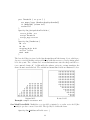
Quick Start: Example OOMMF Session
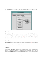
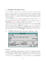
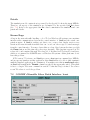
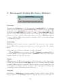
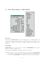
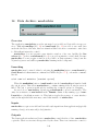
STEP 1: Start up the mmLaunch window.
• At the command prompt, when you are in the OOMMF root directory, type
tclsh oommf.tcl
(The name of the Tcl shell, rendered here as tclsh, may vary between systems. This
matter is discussed in Sec. 2.1.) Alternatively, you may launch oommf.tcl using whatever “point and click” interface is provided by your operating system.
• This will bring up a small window labeled mmLaunch. It will come up in background
mode, so you will get another prompt in your original window, even before the mmLaunch window appears.
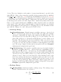
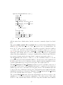
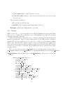
STEP 2: Gain access to other useful windows.
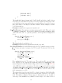
• On the mmLaunch window, check the localhost box, causing a menu of user account
boxes to appear. Check the box corresponding to the account you want to compute on.
(On Windows 9X systems, the user account list may consist of only the faux “oommf”
user account.) This gives a menu of options:
–
–
–
–
–
–
–
mmArchive: to auto-save scalar and vector field data
mmDataTable: to display current values of scalar outputs
mmDisp: to display vector fields
mmGraph: to form x-y plots
mmProbEd: to grab/modify a problem for mmSolve2D or Oxsii
mmSolve2D: to control the 2D solver
Oxsii: to control the 3D solver
• Click on mmDisp, mmGraph, and/or mmDataTable, depending on what form of
output you want. Use mmArchive to save data to disk.
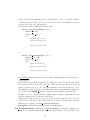
STEP 3a: Run a 2D problem.
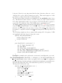
Load problem:
• On the mmLaunch window, click on the mmProbEd button.
• On the mmProbEd window, make menu selection File|Open. . . An Open File
dialog window will appear. On this window:
– Double click in the Path subwindow to change directories. Several sample
problems can be found in the directory oommf/app/mmpe/examples.
– To load a problem, double click on a *.mif file (e.g., prob1.mif) from the list
above the Filter: subwindow.
21
• Modify the problem as desired by clicking on buttons from the main mmProbEd
window (e.g., Material Parameters), and fill out the pop-up forms. A completely
new problem may be defined this way.
• If desired, the defined problem may be stored to disk via the File|Save as. . . menu
selection.
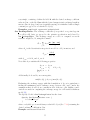
Initialize solver:
• On the mmLaunch window, click on the mmSolve2D button to launch an instance
of the program mmSolve2D.
• Wait for the new solver instance to appear in the Threads column in the mmLaunch window.
• Check the box next to the mmSolve2D entry in the Threads column. A window
containing an mmSolve2D interface will appear.
• On the mmSolve2D window:
– Check Problem Description under Inputs.
– Check mmProbEd under Source Threads.
– Click LoadProblem.
– A status line will indicate the problem is loading.
– When the problem is fully loaded, more buttons appear.
– Check Scheduled Outputs.
– For each desired output (TotalField, Magnetization, and/or DataTable), specify the frequency of update:
1. Check desired output. This will exhibit the possible output destinations under the Destination Threads heading. Output applications such as mmDisp,
mmGraph, and/or mmDataTable must be running to appear in this list.
2. Check the box next to the desired Destination Thread. This will exhibit
Schedule options.
3. Choose a schedule:
∗ Iteration: fill in number and check the box.
∗ ControlPoint: fill in number and check the box.
∗ Interactive: whenever you click corresponding Interactive output button.
Start calculation:
• On the mmSolve2D window, start the calculation with Run (which runs until
problem completion) or Relax (which runs until the next control point is reached).
• If you requested mmDataTable output, check the boxes for the desired quantities
on the mmDataTable window under the Data menu, so that they appear and are
updated as requested in your schedule.
• Similarly, check the box for the desired X, Y1, and Y2 quantities on the mmGraph
window(s) under the X, Y1 and Y2 menus.
22
Save results:
• Vector field data (magnetization and effective field) may be interactively written
to disk using mmDisp, or may be automatically saved via scheduled output to
mmArchive. For example, to save the magnetization state at each control point,
start up an instance of mmArchive and select the ControlPoint check box for
mmArchive on the Magnetization schedule in the solver. This may be done
before starting the calculation. (Control points are points in the simulation where
the applied field is stepped. These are typically equilibrium states, but depending
on the input *.mif file, may be triggered by elapsed simulation time or iteration
count.)
• DataTable data may be saved by sending scheduled output from the solver to
mmArchive, which will automatically save all the data it receives. Alternatively,
mmGraph can perform this function. Schedule output to mmGraph as desired, and use either the interactive or automated save functionality of mmGraph
(Sec. 12). You can setup the solver data scheduling before the calculation is started,
but must wait for the first data point to configure mmGraph before saving any
data. As a workaround, you may configure mmGraph by sending it the initial
solver state interactively, and then use the Options|clear Data menu item in mmGraph to remove the initializing data point.
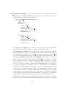
Midcourse control:
• On
–
–
–
–
the mmSolve2D window, buttons can stop and restart the calculation:
Reset: Return to beginning of problem.
LoadProblem: Restart with a new problem.
Run: Apply a sequence of fields until all complete.
Relax: Run the ODE at the current applied field until the next control point
is reached.
– Pause: Click anytime to stop the solver. Continue simulation from paused
point with Run or Relax.
– Field−: Apply the previous field again.
– Field+: Apply the next field in the list.
• Output options can be changed and new output windows opened.
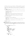
STEP 3b: Run a 3D problem.
Launch solver:
• On the mmLaunch window, click on the Oxsii button to launch an instance of
the program Oxsii.
• Wait for the new solver instance to appear in the Threads column in the mmLaunch window.
23
• Check the box next to the Oxsii entry in the Threads column. A window containing an Oxsii interface will appear.
Load problem:
• On the Oxsii window, select the File|Load. . . menu option. A Load Problem
dialog box will appear. On this window:
– Double click in the Path subwindow to change directories. Several sample
problems can be found in the directory oommf/app/oxs/examples.
– To load a problem, double click on a *.mif file (e.g., stdprob1.mif) from the
list above the Filter: subwindow.
The native input format for the 3D solver is the MIF 2.1 (Sec. 17.1) format, which
must be composed by hand using a plain text editor. (See the Oxs Ext Child
Class (Sec. 7.3) documentation for additional details.) However, MIF 1.1 (i.e., 2D
problem) files are readable by Oxsii, or may be converted to the MIF 2.1 format
using the command line tool mifconvert (Sec. 16.11). mmProbEd also supports
an extension to the MIF 1.1 format, namely MIF 1.2, which provides limited 3D
functionality. MIF 1.2 files may also be read directly by Oxsii.
• The status line in the Oxsii interface window will indicate the problem is loading.
• When the problem is fully loaded, the status line will show “Pause”, and the top
row of buttons (Reload, Reset, . . . ) will become active. Also, the Output list will
fill with available outputs.
• Set up scheduled outputs. For each desired output
1. Select the source from the Output list.
2. Select the receiver from the Destination list.
3. Specify the frequency of update:
– Step: fill in number and check the box.
– Stage: fill in number and check the box.
The items in the Output list will vary depending on the problem that was loaded.
The items in the Destination list reflect the OOMMF data display and archiving
programs currently running.
Start calculation:
• On the Oxsii window, start the calculation with Run, Relax, or Step.
• If you requested mmDataTable output, check the boxes for the desired quantities
on the mmDataTable window under the Data menu, so that they appear and are
updated as requested in your schedule.
• Similarly, check the box for the desired X, Y1, and Y2 quantities on the mmGraph
window(s) under the X, Y1 and Y2 menus.
Save results:
24
• Vector field data (magnetization and effective field) may be interactively written
to disk using mmDisp, or may be automatically saved via scheduled output to
mmArchive. For example, to save the magnetization state at the end of each
problem stage, start up an instance of mmArchive and select the Stage check
box for the Magnetization output, mmArchive destination pair. (Stages denote
points in the simulation where some significant event occurs, such as when an
equilibrium is reached or some preset simulation time index is met. These criteria
are set by the input MIF file.)
• Tabular data may be saved by sending scheduled output from the solver to mmArchive,
which will automatically save all the data it receives. Alternatively, mmGraph
can perform this function. Schedule output to mmGraph as desired, and use either the interactive or automated save functionality of mmGraph (Sec. 12). You
can setup the solver data scheduling before the calculation is started, but must
wait for the first data point to configure mmGraph before saving any data. As
a workaround, you may configure mmGraph by sending it the initial solver state
interactively, and then use the Options|clear Data menu item in mmGraph to
remove the initializing data point.
Midcourse control:
• On
–
–
–
–
–
–
the Oxsii window, buttons can stop and restart the calculation:
Reload: Reload the same file from disk.
Reset: Return to problem start.
Run: Step through all stages until all complete.
Relax: Run until the current stage termination criteria are met.
Step: Do one solver iteration and then pause.
Pause: Click anytime to stop the solver. Continue simulation from paused
point with Run, Relax or Step.
– Stage: Interactively change the current stage index by either typing the desired
stage number (counting from 0) into the Stage entry box or by moving the
associated slider.
• Output options can be changed and new output windows opened. The Send button
in the Oxsii Schedule subwindow is used to interactively send output to the selected
Output + Destination pair.
STEP 4: Exit OOMMF.
• Individual OOMMF applications can be terminated by selecting the File|Exit menu
item from their interface window.
• Selecting File|Exit on the mmLaunch window will close the mmLaunch window, and
also the interface windows for any mmArchive, mmSolve2D, and Oxsii applications.
However, those applications will continue to run in the background, and their interfaces
may be re-displayed by starting a new mmLaunch instance.
25
• To automatically kill all OOMMF applications, select the File|Exit All OOMMF option
from the mmLaunch menu bar.
26
4
OOMMF Architecture Overview
Before describing each of the applications which comprise the OOMMF software, it is helpful
to understand how these applications work together. OOMMF is not structured as a single
program. Instead it is a collection of programs, each specializing in some task needed as
part of a micromagnetic simulation system. An advantage of this modular architecture is
that each program may be improved or even replaced without a need to redesign the entire
system.
The OOMMF programs work together by providing services to one another. The programs communicate over Internet (TCP/IP) connections, even when the programs are running on a common host. An advantage of this design is that distributed operation of OOMMF
programs over a networked collection of hosts is supported in the basic design, and will be
available in a future release.
When two OOMMF applications are in the relationship that one is requesting a service
from the other, it is convenient to introduce some clarifying terminology. Let us refer to
the application that is providing a service as the “server application” and the application
requesting the service as the “client application.” Note that a single application can be both
a server application in one service relationship and a client application in another service
relationship.
Each server application provides its services on a particular Internet port, and needs to
inform potential client applications how to obtain its service. Each client application needs
to be able to look up possible providers of the service it needs. The intermediary which
brings server applications and client applications together is another application called the
“account service directory.” There may be at most one account service directory application
running under the user ID of each user account on a host. Each account service directory
keeps track of all the services provided by OOMMF server applications running under its
user account on its host and the corresponding Internet ports at which those services may be
obtained. OOMMF server applications register their services with the corresponding account
service directory application. OOMMF client applications look up service providers running
under a particular user ID in the corresponding account server directory application.
The account service directory applications simplify the problem of matching servers and
clients, but they do not completely solve it. OOMMF applications still need a mechanism
to find out how to obtain the service of the account service directory! Another application,
called the “host service directory” serves this function. Only one copy of the host service
directory application runs on each host. Its sole purpose is to tell OOMMF applications
where to obtain the services of account service directories on that host. Because only one
copy of this application runs per host, it can provide its service on a well-known port which
is configured into the OOMMF software. By default, this is port 15136. OOMMF software
can be customized (Sec. 2.3.2) to use a different port number.
The account service directory applications perform another task as well. They launch
other programs under the user ID for which they manage service registration. The user
controls the launching of programs through the interface provided by the application mm27
Launch (See Sec. 6), but it is the account service directory application that actually spawns
a subprocess for the new application. Because of this architecture, most OOMMF applications are launched as child processes of an account service directory application. These child
processes inherit their environment from their parent account service directory application,
including their working directory, and other key environment variables, such as DISPLAY.
Each account service directory application sets its working directory to the root directory
of the OOMMF distribution. Future releases of OOMMF software will likely be based on a
revised architecture which alleviates these restrictions.
These service directory applications are vitally important to the operation of the total
OOMMF micromagnetic simulation system. However, it would be easy to overlook them.
They act entirely “behind the scenes” without a user interface window. Furthermore, they
are never launched by the user. When any server application needs to register its service, if
it finds that these service directory applications are not running, it launches new copies of
them. In this way the user can be sure that if any OOMMF server applications are running,
then so are the service directory applications needed to direct clients to its service. After all
server applications terminate, and there are no longer any services registered with a service
directory application, it terminates as well. Similarly, when all service directory applications
terminate, the host service directory application exits.
In the sections which follow, the OOMMF applications are described in terms of the
services they provide and the services they require.
28
5
Command Line Launching
Some of the OOMMF applications are platform-independent Tcl scripts. Some of them
are Tcl scripts that require special platform-dependent interpreters. Others are platformdependent, compiled C++ applications. It is likely that some of them will change status in
later releases of OOMMF. Each of these types of application requires a different command line
for launching. Rather than require all OOMMF users to manage this complexity, we provide
a pair of programs that provide simplified interfaces for launching OOMMF applications.
The first of these is used to launch OOMMF applications from the command line. Because
its function is only to start another program, we refer to this program as the “bootstrap
application.” The bootstrap application is the Tcl script oommf.tcl. In its simplest usage,
it takes a single argument on the command line, the name of the application to launch. For
example, to launch mmGraph (Sec. 12), the command line is:
tclsh oommf.tcl mmGraph
The search for an application matching the name is case-insensitive. (Here, as elsewhere in
this document, the current working directory is assumed to be the OOMMF root directory.
For other cases, adjust the pathname to oommf.tcl as appropriate.) As discussed in Sec. 2.1,
the name of the Tcl shell, rendered here as tclsh, may vary between systems.
If no command line arguments are passed to the bootstrap application, by default it will
launch the application mmLaunch (Sec. 6).
Any command line arguments to the bootstrap application that begin with the character
‘+’ modify its behavior. For a summary of all command line options recognized by the
bootstrap application, run:
tclsh oommf.tcl +help
The command line arguments +bg and +fg control how the bootstrap behaves after
launching the requested application. It can exit immediately after launching the requested
application in background mode (+bg), or it can block until the launched application exits (+fg). Each application registers within the OOMMF system whether it prefers to be
launched in foreground or background mode. If neither option is requested on the command
line, the bootstrap launches the requested application in its preferred mode.
The first command line argument that does not begin with the character + is interpreted
as a specification of which application should be launched. As described above, this is usually
the simple name of an application. When a particular version of an application is required,
though, the bootstrap allows the user to include that requirement as part of the specification.
For example:
tclsh oommf.tcl "mmGraph 1.1"
will guarantee that the instance of the application mmGraph it launches is of at least version
1.1. If no copy of mmGraph satisfying the version requirement can be found, an error is
reported.
29
The rest of the command line arguments that are not recognized by the bootstrap are
passed along as arguments to the application the bootstrap launches. Since the bootstrap
recognizes command line arguments that begin with + and most other applications recognize
command line arguments that begin with -, confusion about which options are provided to
which programs can be avoided. For example,
tclsh oommf.tcl +help mmGraph
prints out help information about the bootstrap and exits without launching mmGraph.
However,
tclsh oommf.tcl mmGraph -help
launches mmGraph with the command line argument -help. mmGraph then displays its
own help message.
Most OOMMF applications accept the standard options listed below. Some of the
OOMMF applications accept additional arguments when launched from the command line,
as documented in the corresponding sections of this manual. The -help command line option
can also be used to view the complete list of available options. When an option argument is
specified as <0|1>, 0 typically means off, no or disable, and 1 means on, yes or enable.
-version Display the version of the application and exit.
-help Display a help message and exit.
-tk <0|1> Disable or enable Tk. Tk must be enabled for an application to display graphical widgets. However, when Tk is enabled on Unix platforms the application is dependent on an X Windows server. If the X Windows server dies, it will kill the application.
Long-running applications that do not inherently use display widgets support disabling
of Tk with -tk 0. Other applications that must use display widgets are unable to run
with the option -tk 0. To run applications that require -tk 1 on a Unix system with
no display, one might use Xvfb13 .
-cwd directory Set the current working directory of the application.
-console Display a console widget in which Tcl commands may be interactively typed into
the application. Useful for debugging.
-nickname <name> Associates the specified name as a nickname for the process. The
string name should contain at least one non-numeric character. Nicknames can also
be set at launch time via the Destination command (Sec. 17.1.2) in MIF 2.x files, or
after a process is running via the nickname (Sec. 16.14) command line application.
Nicknames are used by the MIF 2.x Destination command to associate Oxs output
streams with particular application instances. Multiple -nickname options may be
used to set multiple nicknames. (Technical detail: Nickname functionality is only
available to processes that connect to an account server.)
13
http://www.itworld.com/AppDev/1461/UIR000330xvfb/
30
In addition, those applications which enable Tk accept additional Tk options, such as
-display. See the Tk documentation for details.
The bootstrap application should be infrequently used by most users. The application
mmLaunch (Sec. 6) provides a more convenient graphical interface for launching applications. The main uses for the bootstrap application are launching mmLaunch, launching
pimake, launching programs which make up the OOMMF Batch System (Sec. 10.2) and
other programs that are inherently command line driven, and in circumstances where the user
wishes to precisely control the command line arguments passed to an OOMMF application
or the environment in which an OOMMF application runs.
Platform Issues
On most Unix platforms, if oommf.tcl is marked executable, it may be run directly, i.e.,
without specifying tclsh. This works because the first few lines of the oommf.tcl Tcl script
are:
#!/bin/sh
# \
exec tclsh "$0" ${1+"$@"}
When run, the first tclsh on the execution path is invoked to interpret the oommf.tcl script.
If the Tcl shell program cannot be invoked by the name tclsh on your computer, edit the
first lines of oommf.tcl to use the correct name. Better still, use symbolic links or some
other means to make the Tcl shell program available by the name tclsh. The latter solution
will not be undone by file overwrites from OOMMF upgrades.
If in addition, the directory .../path/to/oommf is in the execution path, the command
line can be as simple as:
oommf.tcl appName
from any working directory.
On Windows platforms, because oommf.tcl has the file extension .tcl, it is normally
associated by Windows with the wish interpreter. The oommf.tcl script has been specially
written so that either tclsh or wish is a suitable interpreter. This means that simply
double-clicking on an icon associated with the file oommf.tcl (say, in Windows Explorer)
will launch the bootstrap application with no arguments. This will result in the default
behavior of launching the application mmLaunch, which is suitable for launching other
OOMMF applications. (If this doesn’t work, refer back to the Windows Options section in
the installation instructions, Sec. 2.4.2.)
31
6
OOMMF Launcher/Control Interface: mmLaunch
Overview
The application mmLaunch launches, monitors, and controls other OOMMF applications.
It is the OOMMF application which is most closely connected to the account service directory
and host service directory applications that run behind the scenes. It also provides user
interfaces to any applications, notably Oxsii (Sec. 7.1) and mmSolve2D (Sec. 10.1), that
do not have their own user interface window.
Launching
mmLaunch should be launched using the bootstrap application (Sec. 5). The command
line is
tclsh oommf.tcl mmLaunch [standard options]
Controls
Upon startup, mmLaunch displays a panel of checkbuttons, one for each host service
directory to which it is connected. In the current release of OOMMF there is only one
checkbutton—localhost. Future releases of mmLaunch will be able to connect to remote
32
hosts as well. If there is no host service directory running on the localhost when mmLaunch is launched, mmLaunch will start one. In that circumstance, there may be some
delay before the localhost check button appears.
Toggling the localhost checkbutton toggles the display of an interface to the host service
directory. The host service directory interface consists of a row of checkbuttons, one for
each account service directory registered with the host service directory. Each checkbutton
is labeled with the user ID of the corresponding account service directory. For most users,
there will be only one checkbutton, labeled with the user’s own account ID, except on
Windows 9X, where the dummy account ID “oommf” may be displayed instead. If there is
no account service directory running for the account under which mmLaunch was launched,
mmLaunch will start one. In that circumstance, there may be some delay before the account
checkbutton appears.
Toggling an account checkbutton toggles the display of an interface to the corresponding
account service directory. The account service directory interface consists of two columns.
The Programs column contains buttons labeled with the names of OOMMF applications
that may be launched under the account managed by this account service directory. Clicking
on one of these buttons launches the corresponding application. Only one click is needed,
though there will be some delay before the launched application displays a window to the
user. Multiple clicks will launch multiple copies of the application. Note: The launching is
actually handled by the account service directory application (Sec. 4), which sets the initial
working directory to the OOMMF root directory.
The Threads column is a list of all the OOMMF applications currently running under
the account that are registered with the account service directory. The list includes both
the application name and an ID number by which multiple copies of the same application
may be distinguished. This ID number is also displayed in the title bar of the corresponding
application’s user interface window. When an application exits, its entry is automatically
removed from the Threads list.
Any of the running applications that do not provide their own interface window will be
displayed in the Threads list with a checkbutton. The checkbutton toggles the display of
an interface which mmLaunch provides on behalf of that application. The only OOMMF
applications currently using this service are the 3D solvers Oxsii and Boxsi (Sec. 7), the 2D
solvers mmSolve2D and batchsolve (Sec. 10), and the archive application mmArchive
(Sec. 14). These interfaces are described in the documentation for the corresponding applications.
The menu selection File|Exit terminates the mmLaunch application, and the File|Exit
All OOMMF selection terminates all applications in the Threads list, and then exits mmLaunch. The menu Help provides the usual help facilities.
33
7
OOMMF eXtensible Solver
The Oxs (OOMMF eXtensible Solver) is an extensible micromagnetic computation engine
capable of solving problems defined on three-dimensional grids of rectangular cells holding
three-dimensional spins. There are two interfaces provided to Oxs: the interactive interface
Oxsii (Sec. 7.1) intended to be controlled primarily through a graphical user interface, and the
batch mode Boxsi (Sec. 7.2), which has extended command line controls making it suitable
for use in shell scripts.
Problem definition for Oxs is accomplished using input files in the MIF 2 format (Sec. 17.1).
This is an extensible format; the standard OOMMF modules are documented in Sec. 7.3 below. Files in the MIF 1.1 and MIF 1.2 formats are also accepted. They are passed to
mifconvert (Sec. 16.11) for conversion to MIF 2 format “on-the-fly.”
Note on Tk dependence: Some MIF 2 problem descriptions rely on external image files;
examples include those using the Oxs ImageAtlas class (Sec. 7.3.1), or those using the MIF 2
ReadFile command with the image translation specification (Sec. 17.1.2). If the image file
is not in the PPM P3 (text) format, then the any2ppm application may be launched to
read and convert the file. Since any2ppm requires Tk, at the time the image file is read a
valid display must be available. See the any2ppm documentation (Sec. 16.1) for details.
7.1
OOMMF eXtensible Solver Interactive Interface: Oxsii
Overview
The application Oxsii is the graphical, interactive user interface to the Oxs micromagnetic
computation engine. Within the OOMMF architecture (see Sec. 4), Oxsii is both a server
and a client application. Oxsii is a client of data table display and storage applications, and
vector field display and storage applications. Oxsii is the server of a solver control service
for which the only client is mmLaunch (Sec. 6). It is through this service that mmLaunch
34
provides a user interface window (shown above) on behalf of Oxsii.
A micromagnetic problem is communicated to Oxsii via a MIF 2 file, which defines a
collection of Oxs Ext objects that comprise the problem model. The problem description
includes a segmentation of the lifetime of the simulation into stages. Stages mark discontinuous changes in model attributes, such as applied fields, and also serve to mark coarse grain
simulation progress. Oxsii provides controls to advance the simulation, stopping between
iterations, between stages, or only when the run is complete. Throughout the simulation,
the user may save and display intermediate results, either interactively or via scheduling
based on iteration and stage counts.
Problem descriptions in the MIF 1.1 and MIF 1.2 formats can also be input. They are
automatically passed to mifconvert (Sec. 16.11) for implicit conversion to MIF 2 format.
Launching
Oxsii may be started either by selecting the Oxsii button on mmLaunch, or from the command line via
tclsh oommf.tcl oxsii [standard options] [-exitondone <0|1>] \
[-nice <0|1>] [-parameters params] [-pause <0|1>] \
[-restart <0|1>] [-threads <count>] [-numanodes <nodes>] [miffile]
where
-exitondone <0|1> Whether to exit after solution of the problem is complete. Default is
to simply await the interactive selection of another problem to be solved.
-nice <0|1> If enabled (i.e., 1), then the program will drop its scheduling priority after
startup. The default is 1, i.e., to yield scheduling priority to other applications.
-parameters params Sets MIF 2 (Sec. 17.1) file parameters. The params argument should
be a list with an even number of arguments, corresponding to name + value pairs. Each
“name” must appear in a Parameter statement (Sec. 17.1.2) in the input MIF file. The
entire name + value list must be quoted so it is presented to Oxsii as a single item
on the command line. For example, if A and Ms appeared in Parameter statements in
the MIF file, then an option like
-parameters "A 13e-12 Ms 800e3"
could be used to set A to 13e-12 and Ms to 800e3. The quoting mechanism is shell/operating
system specific; refer to your system documentation for details.
-pause <0|1> If disabled (i.e., 0), then the program automatically shifts into “Run” mode
after loading the specified miffile. The default is 1, i.e., to “Pause” once the problem
is loaded. This switch has no effect if miffile is not specified.
35
-restart <0|1> Controls the initial setting of the restart flag, and thereby the load restart
behavior of any miffile specified on the command line. The restart flag is described
in the Controls section below. The default value is 0, i.e., no restart.
-threads <count> The option is available on threaded (Sec. 2.3.4) builds of Oxs. The
count parameter is the number of threads to run. The default count value is set by
the oommf thread count value in the config/platforms/ file for your platform, but
may be overridden by the OOMMF THREADS environment variable or this command line
option. In most cases the default count value will equal the number of processing cores
on the system; this can be checked via the command tclsh oommf.tcl +platform.
-numanodes <nodes> This option is available on NUMA-aware (Sec. 2.3.4) builds of
Oxs. The nodes parameter must be either a comma separated list of 0-based node
numbers, the keyword “auto”, or the keyword “none”. In the first case, the numbers refer to memory nodes. These must be passed on the command line as a single
parameter, so either insure there are no spaces in the list, or else protect the spaces
with outlying quotes. For example, -numanodes 2,4,6 or -numanodes "2, 4, 6".
Threads are assigned to the nodes in order, in round-robin fashion. The user can either assign all the system nodes to the Oxsii process, or may restrict Oxsii to run on
a subset of the nodes. In this way the user may reserve specific processing cores for
other processes (or other instances of Oxsii). Although it varies by system, typically
there are multiple processing cores associated with each memory node. If the keyword
“auto” is selected, then the threads are assigned to a fixed node sequence that spans
the entire list of memory nodes. If the keyword “none” is selected, then threads are
not tied to nodes by Oxsii, but are instead assigned by the operating system. In this
last case, over time the operating system is free to move the threads among processors. In the other two cases, each thread is tied to a particular node for the lifetime of
the Oxsii instance. See also the discussion on threading considerations in the Boxsi
documentation.
The default value for nodes is “none”, which allows the operating system to assign
and move threads based on overall system usage. This is also the behavior obtained
when the Oxs build is not NUMA-aware. On the other hand, if a machine is dedicated
primarily to running one instance of Oxsii, then Oxsii will likely run fastest if the
thread count is set to the number of processing cores on the machine, and nodes is set
to “auto”. If you want to run multiple copies of Oxsii simultaneously, or run Oxsii in
parallel with some other application(s), then set the thread count to a number smaller
than the number of processing cores and restrict Oxsii to some subset of the memory
nodes with the -numanodes option and an explicit nodes list.
The environment variable OOMMF NUMANODES may be used to override the default “none”
setting, but is subordinate to the command line setting, if any.
miffile Load and solve the problem found in miffile, which must be either in the MIF 2
format, or convertible to that format by mifconvert. Optional.
36
All the above switches are optional.
Since Oxsii does not present any user interface window of its own, it depends on mmLaunch to provide an interface on its behalf. The entry for an instance of Oxsii in the
Threads column of any running copy of mmLaunch has a checkbutton next to it. This
button toggles the presence of a user interface window through which the user may control
that instance of Oxsii.
Inputs
Unlike mmSolve2D (Sec. 10.1), Oxsii loads problem specifications directly from disk (via
the File|Load... menu selection), rather than through mmProbEd (Sec. 8) or FileSource (Sec. 9). Input files for Oxsii must be either in the MIF 2 (Sec. 17.1) format, or
convertible to that format by the command line tool mifconvert (Sec. 16.11). There are
sample MIF 2 files in the directory oommf/app/oxs/examples. MIF files may be edited with
any plain text editor.
Outputs
Once a problem has been loaded, the scroll box under the Output heading will fill with a list of
available outputs. The contents of this list will depend upon the Oxs Ext objects specified in
the input MIF file. Refer to the documentation for those objects for specific details (Sec. 7.3).
To send output from Oxsii to another OOMMF application, highlight the desired selection
under the Output heading, make the corresponding selection under the Destination heading,
and then specify the output timing under the Schedule heading. Outputs may be scheduled
by the step or stage, and may be sent out interactively by pressing the Send button. The
initial output configuration is set by Destination and Schedule commands in the input
MIF file (Sec. 17.1.2).
Outputs fall under two general categories: scalar (single-valued) outputs and vector field
outputs. The scalar outputs are grouped together as the DataTable entry in the Output scroll
box. Scalar outputs include such items as total and component energies, average magnetization, stage and iteration counts, max torque values. When the DataTable entry is selected,
the Destination box will list all OOMMF applications accepting datatable-style input, i.e.,
all currently running mmDataTable (Sec. 11), mmGraph (Sec. 12), and mmArchive
(Sec. 14) processes.
The vector field outputs include pointwise magnetization, various total and partial magnetic fields, and torques. Unlike the scalar outputs, the vector field outputs are listed individually in the Output scroll box. Allowed destinations for vector field output are running instances of mmDisp (Sec. 13) and mmArchive (Sec. 14). Caution is advised when
scheduling vector field output, especially with large problems, because the output may run
many megabytes.
37
Controls
The File menu button holds five entries: Load, Show Console, Close Interface, Clear Schedule
and Exit Oxsii. File|Load. . . launches a dialog box that allows the user to select an input
MIF problem description file. File|Show Console brings up a Tcl shell console running
off the Oxsii interface Tcl interpreter. This console is intended primary for debugging
purposes. In particular, output from MIF Report commands (Sec. 17.1.2) may be viewed
here. File|Close Interface will remove the interface window from the display, but leaves the
solver running. This effect may also be obtained by deselecting the Oxsii interface button
in the Threads list in mmLaunch. File|Clear Schedule will disable all currently active
output schedules, exactly as if the user clicked through the interactive schedule interface
one output and destination at a time and disabled each schedule-enabling checkbutton. The
final entry, File|Exit Oxsii, terminates the Oxsii solver and closes the interface window.
The Options menu holds two entries: Clear Schedule and Restart Flag. The first clears
all Step and Stage selections from the active output schedules, exactly as if the user clicked
through the interactive schedule interface one output and destination at a time and disabled
each schedule-enabling checkbutton. This control can be used after loading a problem to
override the effect of any Schedule commands in the MIF file. The restart flag controls
problem load behavior. In normal usage, the restart flag is not set and the selected problem
loads and runs from the beginning. Conversely, if the restart flag is set, then when a problem
is loaded a check is made for a restart (checkpoint) file. If the checkpoint file is not found,
then an error is raised. Otherwise, the information in the checkpoint file is used to resume the
problem from the state saved in that file. The restart flag can be set from the Options menu,
the File|Load dialog box, or from the command line. See the Oxs Driver documentation
(Sec. 7.3.5, page 77) for information on checkpoint files.
The Help menu provides the usual help facilities.
The row of buttons immediately below the menu bar provides simulation progress control.
These buttons become active once a problem has been loaded. The first button, Reload,
re-reads the most recent problem MIF input file, re-initializes the solver, and pauses. Reset
is similar, except the file is not re-read. The remaining four buttons, Run, Relax, Step
and Pause place the solver into one of four run-states. In the Pause state, the solver sits
idle awaiting further instructions. If Step is selected, then the solver will move forward one
iteration and then Pause. In Relax mode, the solver takes at least one step, and then runs
until it reaches a stage boundary, at which point the solver is paused. In Run mode, the
solver runs until the end of the problem is reached. Interactive output is available in all
modes; the scheduled outputs occur appropriately as the step and stage counts advance.
Directly below the progress control buttons are two display lines, showing the name of
the input MIF file and the current run-state. Below the run-state Status line is the stage
display and control bar. The simulation stage may be changed at any time by dragging the
scroll bar or by typing the desired stage number into the text display box to the left of the
scroll bar. Valid stage numbers are integers from 0 to N − 1, where N is the number of
stages specified by the MIF input file.
38
Details
The simulation model construction is governed by the Specify blocks in the input MIF file.
Therefore, all aspects of the simulation are determined by the specified Oxs Ext classes
(Sec. 7.3). Refer to the appropriate Oxs Ext class documentation for simulation and computational details.
Known Bugs
A bug in the network traffic handling code of Tcl on Windows 9X systems can sometimes
interfere with communications between the control interface of Oxsii and the actual computation engine. If Oxsii is sending out data to two or more data display services every
iteration, the network traffic from that data can “crowd out” the receipt of control messages
from the control interface. You may observe this as a long delay between the time you click
the Pause button and the time the solver stops iterating. This bug first appeared in Tcl
release 8.0.3, and remained through Tcl release 8.1.1. It is fixed in Tcl releases 8.2 and later,
which we recommend for OOMMF users on Windows 9X systems. Other platforms do not
have this problem.
If Tcl version 7.5 is in use, and Oxsii processes a Destination command in a MIF file,
and in response launches another application, then Oxsii will not be able to fully terminate
until the launched application also terminates. You might notice this in mmLaunch where
an Oxsii will remain in the Threads column long after it has apparently exited. This glitch
is due to a bug in Tcl’s exec command in version 7.5 that has long been fixed. Use a more
recent Tcl release to avoid the problem.
7.2
OOMMF eXtensible Solver Batch Interface: boxsi
39
Overview
The application Boxsi provides a batch mode interface to the Oxs micromagnetic computation engine. A restricted graphical interface is provided, but Boxsi is primarily intended
to be controlled by command line arguments, and launched by the user either directly from
the shell prompt or from inside a batch file.
Within the OOMMF architecture (see Sec. 4), Boxsi is both a server and a client application. It is a client of data table display and storage applications, and vector field display
and storage applications. Boxsi is the server of a solver control service for which the only
client is mmLaunch (Sec. 6). It is through this service that mmLaunch provides a user
interface window (shown above) on behalf of Boxsi.
A micromagnetic problem is communicated to Boxsi through a MIF 2 file specified on
the command line and loaded from disk. The MIF 1.x formats are also accepted; they are
converted to the MIF 2 format by an automatic call to mifconvert (Sec. 16.11).
Launching
Boxsi must be started from the command line. The syntax is
tclsh oommf.tcl boxsi [standard options] [-exitondone <0|1>] \
[-kill tags] [-nice <0|1>] [-parameters params] [-pause <0|1>] \
[-restart <0|1|2>] [-threads <count>] [-numanodes <nodes>] miffile
where
-exitondone <0|1> Whether to exit after solution of the problem is complete, or to await
the interactive selection of the File|Exit command. The default is 1, i.e., automatically
exit when done.
-kill tags On termination, sends requests to other applications to shutdown too. The tags
argument should be either a list of destination tags (which are declared by Destination
commands, Sec. 17.1.2) from the input MIF file, or else the keyword all, which is
interpreted to mean all the destination tags.
-nice <0|1> If enabled (i.e., 1), then the program will drop its scheduling priority after
startup. The default is 0, i.e., to retain its original scheduling priority.
-parameters params Sets MIF 2 (Sec. 17.1) file parameters. The params argument should
be a list with an even number of arguments, corresponding to name + value pairs. Each
“name” must appear in a Parameter statement (Sec. 17.1.2) in the input MIF file. The
entire name + value list must be quoted so it is presented to Boxsi as a single item
on the command line. For example, if A and Ms appeared in Parameter statements in
the MIF file, then an option like
-parameters "A 13e-12 Ms 800e3"
40
could be used to set A to 13e-12 and Ms to 800e3. The quoting mechanism is shell/operating
system specific; refer to your system documentation for details.
-pause <0|1> If enabled (i.e., 1), then the program automatically pauses after loading
the specified problem file. The default is 0, i.e., to automatically move into “Run”
mode once the problem is loaded.
-restart <0|1|2> If the restart option is 0 (the default), then the problem loads and runs
from the beginning. If set to 1, then when loading the problem a check is made for a
pre-existing restart (checkpoint) file. If one is found, then the problem resumes from
the state saved in that file. If no checkpoint file is found, then an error is raised. If the
restart option is set to 2, then a checkpoint file is used if one can be found, but if not
then the problem loads and runs from the beginning without raising an error. See the
Oxs Driver documentation (Sec. 7.3.5, page 77) for information on checkpoint files.
-threads <count> The option is available on threaded (Sec. 2.3.4) builds of Oxs. The
count parameter is the number of threads to run. The default count value is set by
the oommf thread count value in the config/platforms/ file for your platform, but
may be overridden by the OOMMF THREADS environment variable or this command line
option. In most cases the default count value will equal the number of processing cores
on the system; this can be checked via the command tclsh oommf.tcl +platform.
-numanodes <nodes> This option is available on NUMA-aware (Sec. 2.3.4) builds of
Oxs. The nodes parameter must be either a comma separated list of 0-based node
numbers, the keyword “auto”, or the keyword “none”. In the first case, the numbers refer to memory nodes. These must be passed on the command line as a single
parameter, so either insure there are no spaces in the list, or else protect the spaces
with outlying quotes. For example, -numanodes 2,4,6 or -numanodes "2, 4, 6".
Threads are assigned to the nodes in order, in round-robin fashion. The user can either assign all the system nodes to the Boxsi process, or may restrict Boxsi to run
on a subset of the nodes. In this way the user may reserve specific processing cores for
other processes (or other instances of Boxsi). Although it varies by system, typically
there are multiple processing cores associated with each memory node. If the keyword
“auto” is selected, then the threads are assigned to a fixed node sequence that spans
the entire list of memory nodes. If the keyword “none” is selected, then threads are
not tied to nodes by Boxsi, but are instead assigned by the operating system. In this
last case, over time the operating system is free to move the threads among processors.
In the other two cases, each thread is tied to a particular node for the lifetime of the
Boxsi instance. See also the discussion on threading considerations below.
The default value for nodes is “none”, which allows the operating system to assign
and move threads based on overall system usage. This is also the behavior obtained
when the Oxs build is not NUMA-aware. On the other hand, if a machine is dedicated
primarily to running one instance of Boxsi, then Boxsi will likely run fastest if the
41
thread count is set to the number of processing cores on the machine, and nodes is set
to “auto”. If you want to run multiple copies of Boxsi simultaneously, or run Boxsi in
parallel with some other application(s), then set the thread count to a number smaller
than the number of processing cores and restrict Boxsi to some subset of the memory
nodes with the -numanodes option and an explicit nodes list.
The environment variable OOMMF NUMANODES may be used to override the default “none”
setting, but is subordinate to the command line setting, if any.
miffile Load and solve the problem found in miffile, which must be either in the MIF 2
format, or convertible to that format by mifconvert. Required.
Although Boxsi cannot be launched by mmLaunch, nonetheless a limited graphical
interactive interface for Boxsi is provided through mmLaunch, in the same manner as is
done for Oxsii. Each running instance of Boxsi is included in the Threads list of mmLaunch, along with a checkbutton. This button toggles the presence of a user interface
window.
Inputs
Boxsi loads problem specifications directly from disk as requested on the command line.
The format for these files is the MIF 2 (Sec. 17.1) format, the same as used by the Oxsii
interactive interface. The MIF 1.1 and MIF 1.2 formats used by the 2D solver mmSolve2D
can also be input to Boxsi, which will automatically call the command line tool mifconvert
(Sec. 16.11) to convert from the MIF 1.x format to the MIF 2 format “on-the-fly.” Sample
MIF 2 files can be found in the directory oommf/app/oxs/examples.
Outputs
The lower panel of the Boxsi interactive interface presents Output, Destination, and Schedule sub-windows that display the current output configuration and allow interactive modification of that configuration. These controls are identical to those in the Oxsii user interface;
refer to the Oxsii documentation (Sec. 7.1) for details. The only difference between Boxsi
and Oxsii with respect to outputs is that in practice Boxsi tends to rely primarily on
Destination and Schedule commands in the input MIF file (Sec. 17.1.2) to setup the output configuration. The interactive output interface is used for incidental runtime monitoring
of the job.
Controls
The runtime controls provided by the Boxsi interactive interface are a restricted subset of
those available in the Oxsii interface. If the runtime controls provided by Boxsi are found
to be insufficient for a given task, consider using Oxsii instead.
42
The File menu holds 4 entries: Show Console, Close Interface, Clear Schedule, and Exit
Oxsii. File|Show Console brings up a Tcl shell console running off the Boxsi interface Tcl
interpreter. This console is intended primary for debugging purposes. File|Close Interface
will remove the interface window from the display, but leaves the solver running. This
effect may also be obtained by deselecting the Boxsi interface button in the Threads list
in mmLaunch. File|Clear Schedule will disable all currently active output schedules,
exactly as if the user clicked through the interactive schedule interface one output and
destination at a time and disabled each schedule-enabling checkbutton. The final entry,
File|Exit Boxsi, terminates the Boxsi solver and closes the interface window. Note that
there is no File|Load. . . menu item; the problem specification file must be declared on the
Boxsi command line.
The Help menu provides the usual help facilities.
The row of buttons immediately below the menu bar provides simulation progress control. These buttons—Run, Relax, Step and Pause—become active once the micromagnetic
problem has been initialized. These buttons allow the user to change the run state of the
solver. In the Pause state, the solver sits idle awaiting further instructions. If Step is selected, then the solver will move forward one iteration and then Pause. In Relax mode, the
solver takes at least one step, and then runs until it reaches a stage boundary, at which point
the solver is paused. In Run mode, the solver runs until the end of the problem is reached.
When the problem end is reached, the solver will either pause or exit, depending upon the
setting of the -exitondone command line option.
Normally the solver progresses automatically from problem initialization into Run mode,
but this can be changed by the -pause command line switch. Interactive output is available
in all modes; the scheduled outputs occur appropriately as the step and stage counts advance.
Directly below the run state control buttons are three display lines, showing the name
of the input MIF file, the current run-state, and the current stage number/maximum stage
number. Both stage numbers are 0-indexed.
Details
As with Oxsii, the simulation model construction is governed by the Specify blocks in the
input MIF file, and all aspects of the simulation are determined by the specified Oxs Ext
classes (Sec. 7.3). Refer to the appropriate Oxs Ext class documentation for simulation and
computational details.
Threading considerations
As an example, suppose you are running on a four dual-core processor box, where each of the
four processors is connected to a separate memory node. In other words, there are eight cores
in total, and each pair of cores shares a memory node. Further assume that the processors
are connected via point-to-point links such as AMD’s HyperTransport or Intel’s QuickPath
Interconnect.
43
If you want to run a single instance of Boxsi as quickly as possible, you might use the
-threads 8 option, which, assuming the default value of -numanodes none is in effect, would
allow the operating system to schedule the eight threads among the system’s eight cores as
it sees fit. Or, you might reduce the thread count to reserve one or more cores for other
applications. If the job is long running, however, you may find that the operating system
tries to run multiple threads on a single core—perhaps in order to leave other cores idle so
that they can be shut down to save energy. Or, the operating system may move threads
away from the memory node where they have allocated memory, which effectively reduces
memory bandwidth. In such cases you might want to launch Boxsi with the -numanodes
auto option. This overrides the operating systems preferences, and ties threads to particular
memory nodes for the lifetime of the process. (On Linux boxes, you should also check the
“cpu frequency governor” selection and settings.)
If you want to run two instances of Boxsi concurrently, you might launch each with the
-threads 4 option, so that each job has four threads for the operating system to schedule.
If you don’t like the default scheduling by the operating system, you can use the -numanodes
option, but what you don’t want to do is launch two jobs with -numanodes auto, because
the “auto” option assigns threads to memory nodes from a fixed sequence list, so both jobs
will be assigned to the same nodes. Instead, you should manually assign the nodes, with a
different set to each job. For example, you may launch the first job with -numanodes 0,1
and the second job with -numanodes 2,3. One point to keep in mind when assigning nodes
is that some node pairs are “closer” (with respect to memory latency and bandwidth) than
others. For example, memory node 0 and memory node 1 may be directly connected via a
point-to-point link, so that data can be transferred in a single “hop.” But sending data from
node 0 to node 2 may require two hops (from node 0 to node 1, and then from node 1 to
node 2). In this case -numanodes 0,1 will probably run faster than -numanodes 0,2.
The -numanodes option is only available on Linux boxes if the “numactl” and “numactldevel” packages are installed. The numactl command itself can be used to tie jobs to
particular memory nodes, similar to the boxsi -numanodes option, except that -numanodes
ties threads whereas numactl ties jobs. The numactl --hardware command will tell you
how many memory nodes are in the system, and also reports a measure of the (memory
latency and bandwidth) distance between nodes. This information can be used in selecting
nodes for the boxsi -numanodes option, but in practice the distance information reported by
numactl is often not reliable. For best results one should experiment with different settings,
or run memory bandwidth tests with different node pairs.
Known Bugs
Boxsi suffers from the same Windows 9X Tcl network traffic bug as Oxsii. OOMMF users
on Windows 9X systems are encouraged to upgrade to Tcl 8.2 or later.
44
7.3
Standard Oxs Ext Child Classes
An Oxs simulation is built as a collection of Oxs Ext (Oxs Extension) objects. These are
defined via Specify blocks in the input MIF 2 file (Sec. 17.1). The reader will find the
information and sample MIF file, Fig. 7, provided in that section to be a helpful adjunct to
the material presented below. Addition example MIF 2 files can be found in the directory
oommf/app/oxs/examples.
This section describes the Oxs Ext classes available in the standard OOMMF distribution,
including documentation of their Specify block initialization strings, and a list of some sample
MIF files from the oommf/app/oxs/examples directory that use the class. The standard
Oxs Ext objects, i.e., those that are distributed with OOMMF, can be identified by the Oxs
prefix in their names. Additional Oxs Ext classes may be available on your system. Check
local documentation for details.
In the following presentation, the Oxs Ext classes are organized into 8 categories: atlases,
meshes, energies, evolvers, drivers, scalar field objects, vector field objects, and MIF support
classes. The following Oxs Ext classes are currently available:
• Atlases
Oxs BoxAtlas
Oxs MultiAtlas
Oxs EllipsoidAtlas
Oxs ImageAtlas
Oxs ScriptAtlas
• Meshes
Oxs RectangularMesh
• Energies
Oxs CubicAnisotropy
Oxs Exchange6Ngbr
Oxs FixedZeeman
Oxs ScriptUZeeman
Oxs StageZeeman
Oxs TwoSurfaceExchange
Oxs UniformExchange
Oxs
Oxs
Oxs
Oxs
Oxs
Oxs
Oxs
• Evolvers
Oxs CGEvolve
Oxs RungeKuttaEvolve
Oxs EulerEvolve
Oxs SpinXferEvolve
• Drivers
Oxs MinDriver
Oxs TimeDriver
• Scalar Field Objects
Oxs AtlasScalarField
Oxs RandomScalarField
Oxs UniformScalarField
Oxs ScriptOrientScalarField
Oxs AffineTransformScalarField
Oxs
Oxs
Oxs
Oxs
Oxs
45
Demag
ExchangePtwise
RandomSiteExchange
SimpleDemag
TransformZeeman
UniaxialAnisotropy
UZeeman
LinearScalarField
ScriptScalarField
VecMagScalarField
AffineOrientScalarField
ImageScalarField
• Vector Field Objects
Oxs AtlasVectorField
Oxs PlaneRandomVectorField
Oxs ScriptVectorField
Oxs ScriptOrientVectorField
Oxs AffineTransformVectorField
Oxs ImageVectorField
Oxs
Oxs
Oxs
Oxs
Oxs
FileVectorField
RandomVectorField
UniformVectorField
AffineOrientVectorField
MaskVectorField
• MIF Support Classes
Oxs LabelValue
7.3.1
Atlases
Geometric volumes of spaces are specified in Oxs via atlases, which divide their domain into
one or more disjoint subsets called regions. Included in each atlas definition is the atlas
bounding box, which is an axes parallel rectangular parallelepiped containing all the regions.
There is also the special universe region, which consists of all points outside the regions
specified in the atlas. The universe region is not considered to be part of any atlas, and the
universe keyword should not be used to label any of the atlas regions.
The most commonly used atlas is the simple Oxs BoxAtlas. For combining multiple
atlases, use Oxs MultiAtlas.
Oxs BoxAtlas: An axes parallel rectangular parallelepiped, containing a single region that
is coterminous with the atlas itself. The specify block has the form
Specify Oxs BoxAtlas:atlasname {
xrange { xmin xmax }
yrange { ymin ymax }
zrange { zmin zmax }
name regionname
}
where xmin, xmax, . . . are coordinates in meters, specifying the extents of the volume
being defined. The regionname label specifies the name assigned to the region contained
in the atlas. The name entry is optional; if not specified then the region name is taken
from the object instance name, i.e., atlasname.
Examples: sample.mif, cgtest.mif.
Oxs ImageAtlas: This class is designed to allow an image file to be used to define regions in terms of colors in the image. It is intended for use in conjunction with the
Oxs AtlasScalarField and Oxs AtlasVectorField classes in circumstances where
a small number of distinct species (materials) are being modeled. This provides a
generalization of the mask file functionality of the 2D solver (Sec. 17.3.3).
46
For situations requiring continuous variation in material parameters, the script field
classes should be used in conjunction with the ReadFile MIF extension command.
See the ColorField sample proc in the ReadFile documentation in Sec. 17.1.2 for an
example of this technique.
The Oxs ImageAtlas Specify block has the following form:
Specify Oxs ImageAtlas:name {
xrange { xmin xmax }
yrange { ymin ymax }
zrange { zmin zmax }
viewplane view
image pic
colormap {
color-1 region name
color-2 region name
...
color-n region name
}
matcherror max color distance
}
The xrange, yrange, zrange entries specify the extent of the atlas, in meters. The
viewplane view value should be one of the three two-letter codes xy, zx or yz, which
specify the mapping of the horizontal and vertical axes of the image respectively to axes
in the simulation. The image is scaled as necessary along each dimension to match the
atlas extents along the corresponding axes. The image is overlaid through the entire
depth of the perpendicular dimension, i.e., along the axis absent from the viewplane
specification. The Oxs ImageAtlas class can be used inside a Oxs MultiAtlas object
to specify regions in a multilayer structure.
The image entry specifies the name of the image file to use. If the file path is relative,
then it will be taken with respect to the directory containing the MIF file. The image
format may be any of those recognized by any2ppm (Sec. 16.1). The file will be read
directly by Oxs if it is in the P3 or P6 PPM formats, otherwise any2ppm will be
automatically launched to perform the conversion.
The colormap value is an even length list of color + region name pairs. The colors
may be specified in any of several ways. The most explicit is to use one of the Tk
numeric formats, #rgb, #rrggbb, #rrrgggbbb or #rrrrggggbbbb, where each r, g, and
b is one hex digit (i.e., 0-9 or A-F) representing the red, green and blue components
of the color, respectively. For example, #F00 is bright (full-scale) red, #800 would be
a darker red, while #FF0 and #FFFF00 would both be bright yellow. Refer to the
Tk GetColor documentation for details. For shades of gray the special notation grayD
or greyD is available, where D is a decimal value between 0 and 100, e.g., grey0 is
47
black and grey100 is white. Alternatively, one may use any of the symbolic names
defined in the oommf/config/colors.config file, such as red, white and skyblue.
When comparing symbolic names, spaces and capitalization are ignored. The list of
symbolic names can be extended by adding additional files to the Color filename
option in the options.tcl customization file (Sec. 2.3.2). Finally, one color in the
colormap list may optionally be the special keyword “default”. All pixels that don’t
match any of the other specified colors (as determined by the matcherror option) are
assigned to region paired with default.
Each of the specified colors should be distinct, but the region names are allowed to be
repeated as desired. The region names may be chosen arbitrarily, except the special
keyword “universe” is reserved for points not in any of the regions. This includes all
points outside the atlas bounding box defined by the xrange, yrange, zrange entries,
but may also include points inside that boundary.
Pixels in the image are assigned to regions by comparing the color of the pixel to the
list of colors specified in colormap. If the pixel color is closer to a colormap color than
max color distance, then the colors are considered matched. If a pixel color matches
exactly one colormap color, then the pixel is assigned to the corresponding region. If
a pixel color matches more than one colormap color, the pixel is assigned to the region
corresponding to the closest match. If a pixel color doesn’t match any of the colormap
colors, then it is assigned to the default region, which is the region paired with the
“default” keyword. If default does not explicitly appear in the colormap colors list,
then universe is made the default region.
To calculate the distance between two colors, each color is first converted to a scaled
triplet of floating point red, green, and blue values, (r, g, b), where each component
lies in the interval [0, 1], with (0, 0, 0) representing black and (1, 1, 1) representing
white. For example, (0, 0, 1) is bright blue. Given two colors in this representation, the
distance is computed using the standard Euclidean norm with uniform weights, i.e.,
the distance between (r1 , g1 , b1 ) and (r2 , g2 , b2 ) and is
q
(r1 − r2 )2 + (g1 − g2 )2 + (b1 − b2 )2 .
Since the difference
√ in any one component is at most 1, the distance between any two
colors is at most 3.
As explained above, two colors are considered to match if the distance between them
is less than the specified matcherror value. If max color distance is sufficiently small,
then it may easily happen that a pixel’s color does not match any of the specified
region colors, so the pixel would be √
assigned to the default region. On the other hand,
if max color distance is larger than 3, then all colors will match, and no pixels will be
assigned to the default region. If matcherror is not specified, then the default value
for max color distance is 3, which means all colors match.
The following example should help clarify these matters.
48
Specify Oxs_ImageAtlas:atlas {
xrange { 0 400e-9 }
yrange { 0 200e-9 }
zrange { 0 20e-9 }
image mypic.gif
viewplane "xy"
colormap {
blue
cobalt
red
permalloy
green universe
default cobalt
}
matcherror .1
}
Blue pixels get mapped to the “cobalt” region and red pixels to the “permalloy” region.
Green pixels are mapped to the “universe” non-region, which means they are considered
to be outside the atlas entirely. This is a fine point, but comes into play when atlases
with overlapping bounding boxes are brought together inside an Oxs MultiAtlas. To
which region would an orange pixel be assigned? The scaled triplet representation for
orange is (1, 0.647, 0), so the distance to blue is 1.191, the distance to red is 0.647,
and the distance to green is 1.06. Thus the closest color is red, but 0.647 is outside
the matcherror setting of 0.1, so orange doesn’t match any of the colors and is hence
assigned to the default region, which in this case is cobalt. On the other hand, if
matcherror had been set to say 1, then orange and red would match and orange
would be assigned to the permalloy region.
Pixels with colors that are equidistant to and match more than one color in the colormap will be assigned to one of the closest color regions. The user should not rely on
any particular selection, that is to say, the explicit matching procedure in this case is
not defined.
Examples: imageatlas.mif, grill.mif.
Oxs MultiAtlas: This atlas is built up as an ordered list of other atlases. The set of regions
defined by the Oxs MultiAtlas is the union of the regions of all the atlases contained
therein. The sub-atlases need not be disjoint, however each point is assigned to the
region in the first sub-atlas in the list that contains it, so the regions defined by the
Oxs MultiAtlas are effectively disjoint.
49
The Oxs MultiAtlas specify block has the form
Specify Oxs MultiAtlas:name {
atlas
atlas 1 spec
atlas
atlas 2 spec
...
xrange { xmin xmax }
yrange { ymin ymax }
zrange { zmin zmax }
}
Each atlas spec may be either a reference to an atlas defined earlier and outside the
current Specify block, or else an inline, embedded atlas definition. The bounding box
xrange, yrange and zrange specifications are each optional. If not specified the
corresponding range for the atlas bounding box is taken from the minimal bounding
box containing all the sub-atlases.
If the atlases are not disjoint, then the regions as defined by an Oxs MultiAtlas can
be somewhat different from those of the individual component atlases. For example,
suppose regionA is a rectangular region in atlasA with corner points (5,5,0) and
(10,10,10), and regionB is a rectangular region in atlasB with corner points (0,0,0) and
(10,10,10). When composed in the order atlasA, atlasB inside an Oxs MultiAtlas,
regionA reported by the Oxs MultiAtlas will be the same as regionA reported by
atlasA, but regionB as reported by the Oxs MultiAtlas will be the “L” shaped
volume of those points in atlasB’s regionB not inside regionA. If the Oxs MultiAtlas
is constructed with atlasB first and atlasA second, then regionB as reported by the
Oxs MultiAtlas would agree with that reported by atlasB, but regionA would be
empty.
NOTE: The attributes key label (cf. Sec. 17.1.3.5) is not supported by this class.
Examples: manyregions-multiatlas.mif, spinvalve.mif, spinvalve-af.mif, yoyo.mif.
Oxs ScriptAtlas: An atlas where the regions are defined via a Tcl script. The specify
block has the form
Specify Oxs ScriptAtlas:name {
xrange { xmin xmax }
yrange { ymin ymax }
zrange { zmin zmax }
regions { rname 1 rname 2 . . . rname n }
script args { args request }
script Tcl script
}
50
Here xmin, xmax, . . . are coordinates in meters, specifying the extents of the axesparallel rectangular parallelepiped enclosing the total volume being identified. This
volume is subdivided into n sub-regions, using the names as given in the regions list.
The script is used to assign points to the various regions. Appended to the script are
the arguments requested by script args, in the manner explained in the User Defined
Support Procedures section (Sec. 17.1.3.6) of the MIF 2 file format documentation.
The value args request should be a subset of {relpt rawpt minpt maxpt span}. If
script args is not specified, the default value relpt is used. When executed, the
return value from the script should be an integer in the range 1 to n, indicating the
user-defined region in which the point lies, or else 0 if the point is not in any of the
n regions. Region index 0 is reserved for the implicit “universe” region, which is allencompassing. The following example may help clarify the discussion:
proc Octs { cellsize x y z xmin ymin zmin xmax ymax zmax } {
set xindex [expr {int(floor(($x-$xmin)/$cellsize))}]
set yindex [expr {int(floor(($y-$ymin)/$cellsize))}]
set zindex [expr {int(floor(($z-$zmin)/$cellsize))}]
set octant [expr {1+$xindex+2*$yindex+4*$zindex}]
if {$octant<1 || $octant>8} {
return 0
}
return $octant
}
Specify Oxs_ScriptAtlas:octant {
xrange {-20e-9 20e-9}
yrange {-20e-9 20e-9}
zrange {-20e-9 20e-9}
regions { VIII V VII VI IV I III II }
script_args { rawpt minpt maxpt }
script { Octs 20e-9 }
}
This atlas divides the rectangular volume between (−20, −20, −20) and (20, 20, 20)
(nm) into eight regions, corresponding to the standard octants, I through VIII. The
Octs Tcl procedure returns a value between 1 and 8, with 1 corresponding to octant
VIII and 8 to octant II. The canonical octant ordering starts with I as the +x, +y, +z
space, proceeds counterclockwise in the +z half-space, and concludes in the −z halfspace with V directly beneath I, VI beneath II, etc. The ordering computed algorithmically in Octs starts with 1 for the −x, −y, −z space, 2 for the +x, −y, −z space, 3
for the −x, +y, −z space, etc. The conversion between the two systems is accomplished
by the ordering of the regions list.
Examples: manyregions-scriptatlas.mif, octant.mif, tclshapes.mif, diskarray.mif,
ellipsoid-atlasproc.mif.
51
Oxs EllipsoidAtlas: Defines an ellipsoidal region with axes parallel to the coordinate axes.
This functionality can be obtained using the Oxs ScriptAtlas class with an appropriate Tcl script, but this class is somewhat easier to use and faster. The Specify block
has the form
Specify Oxs EllipsoidAtlas:atlasname {
xrange { xmin xmax }
yrange { ymin ymax }
zrange { zmin zmax }
name regionname
}
Here xmin, xmax, . . . are coordinates in meters, specifying the bounding box for the
ellipsoid. The layout of the Specify block is exactly the same as for the Oxs BoxAtlas
class, except that in this case the named region is not the whole bounding box but
rather that subvolume that is the interior of the ellipsoid inscribed inside the bounding
box. Points exterior to that ellipsoid are assigned to the “universe” region.
As in the Oxs BoxAtlas case, the regionname entry is optional; if missing, the region
name is taken from the object instance name, i.e., atlasname.
Example: ellipsoid.mif. See also ellipsoid-atlasproc.mif and
ellipsoid-fieldproc.mif for equivalent examples using Tcl scripts.
7.3.2
Meshes
Meshes define the discretization impressed on the simulation. There should be exactly one
mesh declared in a MIF 2 file. The only standard mesh available at present is
Specify Oxs RectangularMesh:name {
cellsize { xstep ystep zstep }
atlas atlas spec
}
This creates an axes parallel rectangular mesh across the entire space covered by atlas.
The mesh sample rates along each axis are specified by cellsize (in meters). The mesh is
cell-based, with the center of the first cell one half step in from the minimal extremal point
(xmin,ymin,ymax) for atlas spec. The name is commonly set to “mesh”, in which case the
mesh object may be referred to by other Oxs Ext objects by the short name :mesh.
Examples: All MIF files contain this class.
7.3.3
Energies
The following subsections describe the available energy terms. In order to be included in
the simulation energy and field calculations, each energy term must be declared in its own,
top-level Specify block, i.e., energy terms should not be declared inline inside other Oxs Ext
52
objects. There is no limitation on the number of energy terms that may be specified in the
input MIF file. Many of these terms have spatially varying parameters that are initialized
via field object spec entries (Sec. 7.3.6) in their Specify initialization block (see Sec. 17.1.3.2).
Outputs: For each magnetization configuration, two standard outputs are provided by
all energy terms: the scalar output “Energy,” which is the total energy in joules contributed
by this energy term, and the vector field output “Field,” which is the pointwise field in A/m.
If the code was compiled with the macro NDEBUG not defined, then there will be an additional
scalar output, “Calc count,” which counts the number of times the term has been calculated
in the current simulation. This is intended for debugging purposes only; this number should
agree with the “Energy calc count” value provided by the evolver.
• Anisotropy Energy
Oxs UniaxialAnisotropy: Uniaxial magneto-crystalline anisotropy. Specify block
takes 2 parameters, the anisotropy direction axis, and either the crystalline
anisotropy constant K1 (in J/m3 ) or the anistropy field Ha (in A/m). The
axis direction is an easy axis if K1 (or Ha) is >0, or is the normal to the easy
plane if K1 (or Ha) is < 0. Both axis and K1/Ha may be varied cellwise across
the mesh. The anisotropy axis direction is initialized with a vector field object,
while K1 or Ha is initialized with a scalar field object. The axis direction must
be non-zero at each point, and will be normalized to unit magnitude before being
used. The energy computed by this term is non-negative in all cases. Examples:
diskarray.mif, stdprob3.mif, grill.mif.
Oxs CubicAnisotropy: Cubic magneto-crystalline anisotropy. Specify block takes 3
parameters, crystalline anisotropy — either as anisotropy constant K1 in J/m3 or
anisotropy field Ha in A/m — and anisotropy directions axis1 and axis2. The
third anisotropy axis is computed as the vector product, axis1 × axis2. The axis
directions are easy axes if K1 (or Ha) is >0, or hard axes if K1 (or Ha) is <0.
All may be varied cellwise across the mesh. K1 or Ha is initialized with a scalar
field object, and the axis directions are initialized with vector field objects. The
axis1 and axis2 directions must be mutually orthogonal and non-zero at each
point. For each cell, if K1 (resp. Ha) is >0 then the computed energy will be nonnegative, else if K1 (resp. Ha) <0 then the computed energy will be non-positive.
Examples: cgtest.mif, sample2.mif, grill.mif.
• Exchange Energy
Oxs Exchange6Ngbr: Standard 6-neighbor exchange energy. The exchange energy
density contribution from cell i is given by
Ei =
X
Aij
j∈Ni
53
mi · (mi − mj )
∆2ij
(1)
where Ni is the set consisting of the 6 cells nearest to cell i, Aij is the exchange
coefficient between cells i and j in J/m, and ∆ij is the discretization step size
between cell i and cell j (in meters).
The Specify block for this term has the form
Specify Oxs Exchange6Ngbr:name {
default A value
atlas atlas spec
A {
region-1 region-1 A11
region-1 region-2 A12
...
region-m region-n Amn
}
}
or
Specify Oxs Exchange6Ngbr:name {
default lex value
atlas atlas spec
les {
region-1 region-1 lex11
region-1 region-2 lex12
...
region-m region-n lexmn
}
}
where
lex specifies the magnetostatic-exchange length, in meters, defined by lex =
q
2A/(µ0 Ms2 ).
In the first case, the A block specifies Aij values on a region by region basis, where
the regions are labels declared by atlas spec. This allows for specification of A both
inside a given region (e.g., Aii ) and along interfaces between regions (e.g., Aij ).
By symmetry, if Aij is specified, then the same value is automatically assigned to
Aji as well. The default A value is applied to any otherwise unassigned Aij .
In the second case, one specifies the magnetostatic-exchange length instead of A,
but the interpretation is otherwise analogous.
Although one may specify Aij (resp. lexij ) for any pair of regions i and j, it is only
required and only active if the region pair are in contact. If long-range exchange
interaction is required, use Oxs TwoSurfaceExchange.
Examples: grill.mif, spinvalve.mif, tclshapes.mif.
Oxs UniformExchange: Similar to Oxs Exchange6Ngbr, except the exchange constant A (or exchange length lex) is uniform across all space. The Specify block is
54
very simple, consisting of either the label A with the desired exchange coefficient
value in J/m, or the label lex with the desired magnetostatic-exchange length in
meters. Since A (resp. lex) is not spatially varying, it is initialized with a simple
constant (as opposed to a scalar field object).
Examples: sample.mif, cgtest.mif, stdprob3.mif.
Oxs ExchangePtwise: The exchange coefficient Ai is specified on a point-by-point
(or cell-by-cell) basis, as opposed to the pairwise specification model used by
Oxs Exchange6Ngbr. The exchange energy at a cell i is computed across its
nearest 6 neighbors, Ni , using the formula
Ei =
X
Aij,eff
j∈Ni
mi · (mi − mj )
∆2ij
where ∆ij is the discretization step size from cell i to cell j in meters, and
Aij,eff =
2Ai Aj
,
Ai + A j
with Aij,eff = 0 if Ai and Aj are 0.
Note that Aij,eff satisfies the following properties:
Aij,eff = Aji,eff
Aij,eff = Ai
if Ai = Aj
lim Aij,eff = 0.
Ai ↓0
Additionally, if Ai and Aj are non-negative,
min(Ai , Aj ) ≤ Aij,eff ≤ max(Ai , Aj ).
Evaluating the exchange energy with this formulation of Aij,eff is equivalent to
finding the minimum possible exchange energy between cells i and j under the
assumption that Ai and Aj are constant in each of the two cells. Similar considerations are made in computing the exchange energy for a 2D variable thickness
model [16].
The Specify block for Oxs ExchangePtwise has the form
Specify Oxs ExchangePtwise:name {
A scalarfield spec
}
where scalarfield spec is an arbitrary scalar field object (Sec. 7.3.6) returning the
desired exchange coefficient in J/m.
Example: antidots-filled.mif.
55
Oxs TwoSurfaceExchange: Provides long-range bilinear and biquadratic exchange.
Typically used to simulate RKKY-style coupling across non-magnetic spacers in
spinvalves. The specify block has the form
Specify Oxs TwoSurfaceExchange:name {
sigma value
sigma2 value
surface1 {
atlas atlas spec
region region label
scalarfield scalarfield spec
scalarvalue fieldvalue
scalarside sign
}
surface2 {
atlas atlas spec
region region label
scalarfield scalarfield spec
scalarvalue fieldvalue
scalarside sign
}
}
Here sigma and sigma2 are the bilinear and biquadratic surface (interfacial)
exchange energies, in J/m2 . Either is optional, with default value 0.
The surface1 and surface2 sub-blocks describe the two interacting surfaces.
Each description consists of 5 name-values pairs, which must be listed in the
order shown. In each sub-block, atlas spec specifies an atlas, and region label
specifies a region in that atlas. These bound the extent of the desired surface. The
following scalarfield, scalarvalue and scalarside entries define a discretized
surface inside the bounding region. Here scalarfield spec references a scalar field
object, fieldvalue should be a floating point value, and sign should be a single
character, either ‘−’ or ‘+’. If sign is ‘−’, then any point for which the scalar field
object takes a value less than or equal to the scalarvalue value is considered to
be “inside” the surface. Conversely, if sign is ‘+’, then any point for which the
scalar field object has value greater than or equal to the scalarvalue value is
considered to be “inside” the surface. The discretized surface determined is the
set of all points on the problem mesh that are in the bounding region, are either
on the surface or lie on the “inside” side of the surface, and have a (nearest-)
neighbor that is on the “outside” side of the surface. A “neighbor” is determined
by the mesh; in a typically rectangular mesh each cell has six neighbors.
In this way, 2 discrete lists of cells representing the two surfaces are obtained.
Each cell from the first list (representing surface1) is then matched with the
56
closest cell from the second list (i.e., from surface2). Note the asymmetry in this
matching process: each cell from the first list is included in exactly one match,
but there may be cells in the second list that are included in many match pairs,
or in none. If the two surfaces are of different sizes, then in practice typically
the smaller will be made the first surface, because this will usually lead to fewer
multiply-matched cells, but this designation is not required.
The resulting exchange energy density at cell i on one surface from matching cell
j on the other is given by
h
Eij =
σ [1 − mi · mj ] + σ2 1 − (mi · mj )2
i
∆ij
where σ and σ2 , respectively, are the bilinear and biquadratic surface exchange
coefficients between the two surfaces, in J/m2 , mi and mj are the normalized, unit
spins (i.e., magnetization directions) at cells i and j, and ∆ij is the discretization
cell size in the direction from cell i towards cell j, in meters. Note that if σ is
negative, then the surfaces will be anti-ferromagnetically coupled. Likewise, if σ2
is negative, then the biquadratic term will favor orthogonal alignment.
The following example produces an antiferromagnetic exchange coupling between
the lower surface of the “top” layer and the upper surface of the “bottom” layer,
across a middle “spacer” layer. The simple Oxs LinearScalarField object is
used here to provide level surfaces that are planes orthogonal to the z-axis. In
practice this example might represent a spinvalve, where the top and bottom
layers would be composed of ferromagnetic material and the middle layer could
be a copper spacer.
Specify Oxs_MultiAtlas:atlas {
atlas { Oxs_BoxAtlas {
name top
xrange {0 500e-9}
yrange {0 250e-9}
zrange {6e-9 9e-9}
} }
atlas { Oxs_BoxAtlas {
name spacer
xrange {0 500e-9}
yrange {0 250e-9}
zrange {3e-9 6e-9}
} }
atlas { Oxs_BoxAtlas {
name bottom
xrange {0 500e-9}
yrange {0 250e-9}
57
zrange {0 3e-9}
} }
}
Specify Oxs_LinearScalarField:zheight {
vector {0 0 1}
norm
1.0
}
Specify Oxs_TwoSurfaceExchange:AF {
sigma -1e-4
surface1 {
atlas :atlas
region bottom
scalarfield :zheight
scalarvalue 3e-9
scalarside }
surface2 {
atlas :atlas
region top
scalarfield :zheight
scalarvalue 6e-9
scalarside +
}
}
Example: spinvalve-af.mif.
Oxs RandomSiteExchange: A randomized exchange energy. The Specify block has
the form
Specify Oxs RandomSiteExchange:name {
linkprob probability
Amin A lower bound
Amax A upper bound
}
Each adjacent pair of cells i, j, is given linkprob probability of having a non-zero
exchange coefficient Aij . Here two cells are adjacent if they lie in each other’s 6neighborhood. If a pair is found to have a non-zero exchange coefficient, then Aij
is drawn uniformly from the range [Amin, Amax]. The exchange energy is computed
using (1), the formula used by the Oxs Exchange6Ngbr energy object. The value
Aij for each pair of cells is determined during problem initialization, and is held
fixed thereafter. The limits A lower bound and A upper bound may be any real
58
numbers; negative values may be used to weaken the exchange interaction arising
from other exchange energy terms. The only restriction is that A lower bound
must not be greater than A upper bound. The linkprob value probability must
lie in the range [0, 1].
Example: randexch.mif.
• Self-Magnetostatic Energy
Oxs Demag: Standard demagnetization energy term, which is built on the assumption that the magnetization is constant in each cell, and computes the average
demagnetization field through the cell using formulae from [2, 15] and convolution via the Fast Fourier Transform. The Specify initialization string should be
an empty string, typically denoted by {}.
Examples: sample.mif, cgtest.mif.
Oxs SimpleDemag: This is the same as the Oxs Demag object, except that the implementation does not use any of the of the symmetries inherent in the demagnetization kernel, or special properties of the Fourier Transform when applied to a
real (non-complex) function. As a result, the source code for this implementation
is considerably simpler than for Oxs Demag, but the run time performance and
memory usage are poorer. Oxs SimpleDemag is included for validation checks,
and as a base for user-defined demagnetization implementations. The Specify
initialization string for Oxs SimpleDemag is an the empty string, i.e., {}.
Example: squarecubic.mif.
• Zeeman Energy
Oxs UZeeman: Uniform (homogeneous) applied field energy. This class is frequently
used for simulating hysteresis loops. The specify block takes an optional multiplier entry, and a required field range list Hrange. The field range list should be
a compound list, with each sublist consisting of 7 elements: the first 3 denote the
x, y, and z components of the start field for the range, the next 3 denote the x,
y, and z components of the end field for the range, and the last element specifies
the number of (linear) steps through the range. If the step count is 0, then the
range consists of the start field only. If the step count is bigger than 0, then the
start field is skipped over if and only if it is the same field that ended the previous
range (if any).
The fields specified in the range entry are nominally in A/m, but these values
are multiplied by multiplier, which may be used to effectively change the units.
For example,
Specify Oxs UZeeman {
multiplier 795.77472
Hrange {
59
{ 0 0 0 10 0 0 2 }
{ 10 0 0 0 0 0 1 }
}
}
The applied field steps between 0 mT, 5 mT, 10 mT and back to 0 mT, for four
stages in total. If the first field in the second range sublist was different from the
second field in the first range sublist, then a step would have been added between
those field values, so five stages would have resulted. In this example, note that
795.77472=0.001/µ0 .
Examples: sample.mif, cgtest.mif, marble.mif.
Oxs FixedZeeman: Non-uniform, non-time varying applied field. This can be used
to simulate a biasing field. The specify block takes one required parameter, which
defines the field, and one optional parameter, which specifies a multiplication
factor.
Specify Oxs FixedZeeman:name {
field vector field spec
multiplier multiplier
}
The default value for multiplier is 1.
Examples: spinvalve.mif, spinvalve-af.mif, yoyo.mif.
Oxs ScriptUZeeman: Spatially uniform applied field, potentially varying as a function of time and stage, determined by a Tcl script. The Specify block has the
form
Specify Oxs ScriptUZeeman:name {
script args { args request }
script Tcl script
multiplier multiplier
stage count number of stages
}
Here script indicates the Tcl script to use. The script is called once each iteration. Appended to the script are the arguments requested by script args, in the
manner explained in the User Defined Support Procedures section (Sec. 17.1.3.6)
of the MIF 2 file format documentation. The value args request should be a subset
of {stage stage time total time}. If script args is not specified, the default
argument list is the complete list in the aforementioned order. The units for the
time arguments are seconds.
The return value from the script should be a 6-tuple of numbers, {Hx, Hy, Hz, dHx,
dHy, dHz}, representing the applied field and the time derivative of the applied
field. The field as a function of time must be differentiable for the duration of
each stage. Discontinuities are permitted between stages. If a time evolver is
60
being used, then it is very important that the time derivative values are correct;
otherwise the evolver will not function properly. This usual symptom of this
problem is a collapse in the time evolution step size.
The field and its time derivative are multiplied by the multiplier value before
use. The final field value should be in A/m; if the Tcl script returns the field
in T, then a multiplier value of 1/µ0 (approx. 795774.72) should be applied to
convert the Tcl result into A/m. The default value for multiplier is 1.
The stage count parameter informs the Oxs Driver (Sec. 7.3.5) as to how many
stages the Oxs ScriptUZeeman object wants. A value of 0 (the default) indicates
that the object is prepared for any range of stages. The stage count value given
here must be compatible with the stage count setting in the driver Specify block
(q.v.).
The following example produces a sinusoidally varying field of frequency 1 GHz
and amplitude 800 A/m, directed along the x-axis.
Specify Oxs_ScriptUZeeman {
script_args total_time
script SineField
}
proc SineField { total_time } {
set PI [expr {4*atan(1.)}]
set Amp 800.0
set Freq [expr {1e9*(2*$PI)}]
set Hx [expr {$Amp*sin($Freq*$total_time)}]
set dHx [expr {$Amp*$Freq*cos($Freq*$total_time)}]
return [list $Hx 0 0 $dHx 0 0]
}
Examples: acsample.mif, pulse.mif, rotate.mif, varalpha.mif, yoyo.mif.
Oxs TransformZeeman: Essentially a combination of the Oxs FixedZeeman and
Oxs ScriptUZeeman classes, where an applied field is produced by applying a
spatially uniform, but time and stage varying linear transform to a spatially varying but temporally static field. The transform is specified by a Tcl script.
The Specify block has the form
Specify Oxs TransformZeeman:name {
field vector field spec
type transform type
script Tcl script
script args { args request }
multiplier multiplier
stage count number of stages
}
61
The field specified by vector field spec is evaluated during problem initialization
and held throughout the life of the problem. On each iteration, the specified
Tcl script is called once. Appended to the script are the arguments requested
by script args, as explained in the User Defined Support Procedures section
(Sec. 17.1.3.6) of the MIF 2 file format documentation. The value for script args
should be a subset of {stage stage time total time}. The default value for
script args is the complete list in the aforementioned order. The time arguments
are specified in seconds.
The script return value should define a 3x3 linear transform and its time derivative. The transform must be differentiable with respect to time throughout
each stage, but is allowed to be discontinuous between stages. As noted in the
Oxs ScriptUZeeman documentation, it is important that the derivative information be correct. The transform is applied pointwise to the fixed field obtained
from vector field spec, which is additionally scaled by multiplier. The multiplier
entry is optional, with default value 1.0.
The type transform type value declares the format of the result returned from the
Tcl script. Recognized formats are identity, diagonal, symmetric and general.
The most flexible is general, which indicates that the return from the Tcl script
is a list of 18 numbers, defining a general 3x3 matrix and its 3x3 matrix of time
derivatives. The matrices are specified in row-major order, i.e., M1,1 , M1,2 , M1,3 ,
M2,1 , M2,2 , . . . . Of course, this is a long list to construct; if the desired transform
is symmetric or diagonal, then the type may be set accordingly to reduce the size
of the Tcl result string. Scripts of the symmetric type return 12 numbers, the 6
upper diagonal entries in row-major order, i.e., M1,1 , M1,2 , M1,3 , M2,2 , M2,3 , M3,3 ,
for both the transformation matrix and its time derivative. Use the diagonal
type for diagonal matrices, in which case the Tcl script result should be a list of
6 numbers.
The simplest transform type is identity, which is the default. This identifies
the transform as the identity matrix, which means that effectively no transform is applied, aside from the multiplier option which is still active. For
the identity transform type, script and script args should not be specified,
and Oxs TransformZeeman becomes a clone of the Oxs FixedZeeman class.
The following example produces a 1000 A/m field that rotates in the xy-plane at
a frequency of 1 GHz:
Specify Oxs_TransformZeeman {
type general
script {Rotate 1e9}
field {0 1000. 0}
}
proc Rotate { freq stage stagetime totaltime } {
global PI
62
set w [expr {$freq*2*$PI}]
set ct [expr {cos($w*$totaltime)}]
set mct [expr {-1*$ct}]
;# "mct" is "minus
set st [expr {sin($w*$totaltime)}]
set mst [expr {-1*$st}]
;# "mst" is "minus
return [list $ct $mst 0 \
$st $ct
0 \
0
0
1 \
[expr {$w*$mst}] [expr {$w*$mct}]
[expr {$w*$ct}] [expr {$w*$mst}]
0
0
cosine (w)t"
sine (w)t"
0 \
0 \
0]
}
This particular effect could be obtained using the Oxs ScriptUZeeman class, because the field is uniform. But the field was taken uniform only to simplify the
example. The vector field spec may be any Oxs vector field object (Sec. 7.3.6).
For example, the base field could be large in the center of the sample, and decay
towards the edges. In that case, the above example would generate an applied
rotating field that is concentrated in the center of the sample.
The stage count parameter informs the Oxs Driver (Sec. 7.3.5) as to how many
stages the Oxs TransformZeeman object wants. A value of 0 (the default) indicates that the object is prepared for any range of stages. The stage count value
given here must be compatible with the stage count setting in the driver Specify
block (q.v.).
Examples: sample2.mif, tickle.mif, rotatecenter.mif.
Oxs StageZeeman: The Oxs StageZeeman class provides spatially varying applied
fields that are updated once per stage. In its general form, the field at each stage
is provided by an Oxs vector field object (Sec. 7.3.6) determined by a user supplied
Tcl script. There is also a simplified interface that accepts a list of vector field
files (Sec. 19), one per stage, that are used to specify the applied field.
The Specify block takes the form
Specify Oxs StageZeeman:name {
script Tcl script
files { list of files }
stage count number of stages
multiplier multiplier
}
The initialization string should specify either script or files, but not both. If
a script is specified, then each time a new stage is started in the simulation,
a Tcl command is formed by appending to Tcl script the 0-based integer stage
number. This command should return a reference to an Oxs VectorField object,
as either the instance name of an object defined via a top-level Specify block
63
elsewhere in the MIF file, or as a two item list consisting of the name of an
Oxs VectorField class and an appropriate initialization string. In the latter case
the Oxs VectorField object will be created as a temporary object via an inlined
Specify call.
The following example should help clarify the use of the script parameter.
Specify Oxs_StageZeeman {
script SlidingFieldSpec
stage_count 11
}
proc SlidingFieldSpec { stage } {
set xcutoff [expr {double($stage)/10.}]
set spec Oxs_ScriptVectorField
lappend spec [subst {
atlas :atlas
script {SlidingField $xcutoff}
}]
return $spec
}
proc SlidingField { xcutoff xrel yrel zrel } {
if {$xrel>$xcutoff} { return [list 0. 0. 0.] }
return [list 2e4 0. 0.]
}
The SlidingFieldSpec proc is used to generate the initialization string for an
Oxs ScriptVectorField vector field object, which in turn uses the SlidingField
proc to specify the applied field on a position-by-position basis. The resulting
field will be 2 × 104 A/m in the positive x-direction at all points with relative
x-coordinate larger than $stage/10., and 0 otherwise. $stage is the stage index,
which here is one of 0, 1, . . . , 10. For example, if $stage is 5, then the left half of
the sample will see a 2 × 104 A/m field directed to the right, and the right half of
the sample will see none. The return value from SlidingFieldSpec in this case
will be
Oxs_ScriptVectorField {
atlas :atlas
script {SlidingField 0.5}
}
The :atlas reference is to an Oxs Atlas object defined elsewhere in the MIF file.
The stage count parameter lets the Oxs Driver (Sec. 7.3.5) know how many
stages the Oxs StageZeeman object wants. A value of 0 indicates that the object
is prepared for any range of stages. Zero is the default value for stage count
64
when using the Tcl script interface. The stage count value given here must be
compatible with the stage count setting in the driver Specify block (q.v.).
The example above made use of two scripts, one to specify the Oxs VectorField
object, and one used internally by the Oxs ScriptVectorField object. But any
Oxs VectorField class may be used, as in the next example.
Specify Oxs_StageZeeman {
script FileField
stage_count 3
}
proc FileField { stage } {
set filelist { field-a.ohf field-b.ohf field-c.ohf }
set spec Oxs_FileVectorField
lappend spec [subst {
atlas :atlas
file [lindex $filelist $stage]
}]
return $spec
}
The FileField proc yields a specification for an Oxs FileVectorField object
that loads one of three files, field-a.ohf, field-b.ohf, or field-c.ohf, depending on the stage number.
Specifying applied fields from a sequence of files is common enough to warrant a
simplified interface. This is the purpose of the files parameter:
Specify Oxs_StageZeeman {
files { field-a.ohf field-b.ohf field-c.ohf }
}
This is essentially equivalent to the preceding example, with two differences. First,
stage count is not needed because Oxs StageZeeman knows the length of the list
of files. You may specify stage count, but the default value is the length of the
files list. This is in contrast to the default value of 0 when using the script
interface. If stage count is set larger than the file list, then the last file is repeated
as necessary to reach the specified size.
The second difference is that no Oxs Atlas is specified when using the files
interface. The Oxs FileVectorField object spatially scales the field read from
the file to match a specified volume. Typically a volume is specified by explicit
reference to an atlas, but with the files interface to Oxs StageZeeman the file
fields are implicitly scaled to match the whole of the meshed simulation volume.
This is the most common case; to obtain a different spatial scaling use the script
interface as illustrated above with a different atlas or an explicit x/y/z-range
specification.
65
The list of files value is interpreted as a grouped list. See the notes in Sec. 17.1.3.3
for details on grouped lists.
The remaining Oxs StageZeeman parameter is multiplier. The value of this
parameter is applied as a scale factor to the field magnitude on a point-by-point
basis. For example, if the field returned by the Oxs VectorField object were
in Oe, instead of the required A/m, then multiplier could be set to 79.5775
to perform the conversion. The direction of the applied field can be reversed by
supplying a negative multiplier value.
Examples: sliding.mif, slidingproc.mif, rotatestage.mif,
rotatecenterstage.mif.
7.3.4
Evolvers
Evolvers are responsible for updating the magnetization configuration from one step to the
next. There are two types of evolvers, time evolvers, which track Landau-Lifshitz-Gilbert dynamics, and minimization evolvers, which locate local minima in the energy surface through
direct minimization techniques. Evolvers are controlled by drivers (Sec. 7.3.5), and must
be matched with the appropriate driver type, i.e., time evolvers must be paired with time
drivers, and minimization evolvers must be paired with minimization drivers. The drivers
hand a magnetization configuration to the evolvers with a request to advance the configuration by one step (also called an iteration). It is the role of the drivers, not the evolvers, to
determine when a simulation stage or run is complete. Specify blocks for evolvers contain
parameters to control all aspects of individual stepwise evolution, but stopping criteria are
communicated in the Specify block of the driver, not the evolver.
There are currently three time evolvers and one minimization evolver in the standard
OOMMF distribution. The time evolvers are Oxs EulerEvolve, Oxs RungeKuttaEvolve,
and Oxs SpinXferEvolve. The minimization evolver is Oxs CGEvolve.
Oxs EulerEvolve: Time evolver implementing a simple first order forward Euler method
with step size control on the Landau-Lifshitz ODE [10, 12]:
dM
|¯
γ |α
(2)
= −|¯
γ | M × Heff −
M × (M × Heff ) ,
dt
Ms
where M is the magnetization, Heff is the effective field, γ¯ is the Landau-Lifshitz
gyromagnetic ratio, and α is the damping constant. The Gilbert form
!
dM
α
dM
= −|γ| M × Heff +
M×
,
dt
Ms
dt
(3)
where γ is the Gilbert gyromagnetic ratio, is mathematically equivalent to the LandauLifshitz form under the relation γ = (1 + α2 ) γ¯ .
The Specify block has the form
66
Specify Oxs EulerEvolve:name {
alpha α
gamma LL γ¯
gamma G γ
do precess precess
min timestep minimum stepsize
max timestep maximum stepsize
fixed spins {
atlas spec
region1 region2 . . .
}
start dm ∆m
error rate rate
absolute step error abs error
relative step error rel error
step headroom headroom
}
All the entries have default values, but the ones most commonly adjusted are listed
first.
The options alpha, gamma LL and gamma G are as in the Landau-Lifshitz-Gilbert
ODE (2), (3), where the units on γ¯ and γ are m/A·s and α is dimensionless. At
most one of γ¯ and γ should be specified. If neither is specified, then the default is
γ = 2.211 × 105 . (Because of the absolute value convention adopted on γ¯ and γ in
(2), (3), the sign given to the value of gamma LL or gamma G in the Specify block is
irrelevant.) The default value for α is 0.5, which is large compared to experimental
values, but allows simulations to converge to equilibria in a reasonable time. However,
for accurate dynamic studies it is important to assign an appropriate value to α.
The do precess value should be either 1 or 0, and determines whether or not the
precession term in the Landau-Lifshitz ODE (i.e., the first term on the righthand side
in (2)) is used. If precess is 0, then precession is disabled and the simulation evolves
towards equilibrium along a steepest descent path. The default value is 1.
The min timestep and max timestep parameters provide soft limits on the size of
steps taken by the evolver. The minimum value may be overridden by the driver if a
smaller step is needed to meet time based stopping criteria. The maximum value will
be ignored if a step of that size would produce a magnetization state numerically indistinguishable from the preceding state. The units for min timestep and max timestep
are seconds. Default values are 0 and 10−10 respectively.
The optional fixed spins entry allows the magnetization in selected regions of the
simulation to be frozen in its initial configuration. The value portion of the entry
should be a list, with the first element of the list being either an inline atlas definition
67
(grouped as a single item), or else the name of a previously defined atlas. The remainder
of the list are names of regions in that atlas for which the magnetization is to be be
fixed, i.e., M(t) = M(0) for all time t for all points in the named regions. Fields and
energies are computed and reported normally across these regions. Although any atlas
may be used, it is frequently convenient to set up an atlas with special regions defined
expressly for this purpose.
The stepsize for the first candidate iteration in the problem run is selected so that the
maximum change in the normalized (i.e., unit) magnetization m is the value specified
by start dm. The units are degrees, with default value 0.01.
The four remaining entries, error rate, absolute step error, relative step error,
and step headroom, control fine points of stepsize selection, and are intended for
advance use only. Given normalized magnetization mi (t) at time t and position i, and
candidate magnetization mi (t + ∆t) at time t + ∆t, the error at position i is estimated
to be
˙ i (t + ∆t) − m
˙ i (t)| ∆t / 2,
Errori = |m
˙ is computed using the Landau-Lifshitz
where the derivative with respect to time, m,
˙ is constant on the interval
ODE (2). First order methods essentially assume that m
˙ at the endpoints of the interval
[t, t + ∆t]; the above formula uses the difference in m
to estimate (guess) how untrue that assumption is.
A candidate step is accepted if the maximum error across all positions i is smaller
˙ max |∆t,
than absolute step error, error rate × ∆t, and relative step error × |m
˙ max | is the maximum value of |m
˙ i | across all i at time t. If the step is
where |m
rejected, then a smaller stepsize is computed that appears to pass the above tests, and
a new candidate step is proposed using that smaller stepsize times step headroom.
Alternatively, if the step is accepted, then the error information is used to determine
the stepsize for the next step, modified in the same manner by step headroom.
The error calculated above is in terms of unit magnetizations, so the natural units
are radians or radians/second. Inside the Specify block, however, the error rate and
absolute step error are specified in degrees/nanosecond and degrees, respectively;
they are converted appropriately inside the code before use. The relative step error
is a dimensionless quantity, representing a proportion between 0 and 1. The error check
controlled by each of these three quantities may be disabled by setting the quantity
value to -1. They are all optional, with default values of -1 for error rate, 0.2 for
absolute step error, and 0.2 for relative step error.
The headroom quantity should lie in the range (0, 1), and controls how conservative the
code will be in stepsize selection. If headroom is too large, then much computation time
will be lost computing candidate steps that fail the error control tests. If headroom
is small, then most candidate steps will pass the error control tests, but computation
time may be wasted calculating more steps than are necessary. The default value for
headroom is 0.85.
68
In addition to the above error control tests, a candidate step will also be rejected if
the total energy, after adjusting for effects due to any time varying external field, is
found to increase. In this case the next candidate stepsize is set to one half the rejected
stepsize.
The Oxs EulerEvolve module provides five scalar outputs and three vector field outputs. The scalar outputs are
• Max dm/dt: maximum |dm/dt|, in degrees per nanosecond; m is the unit
magnetization direction.
• Total energy: in joules.
• Delta E: change in energy between last step and current step, in joules.
• dE/dt: derivative of energy with respect to time, in joules per second.
• Energy calc count: number of times total energy has been calculated.
The vector field outputs are
• Total field: total effective field H in A/m.
• mxH: torque in A/m; m is the unit magnetization direction, H is the total
effective field.
• dm/dt: derivative of spin m with respect to time, in radians per second.
Example: octant.mif.
Oxs RungeKuttaEvolve: Time evolver implementing several Runge-Kutta methods for
integrating the Landau-Lifshitz-Gilbert ODE (2), (3), with step size control. In most
cases it will greatly outperform the Oxs EulerEvolve class. The Specify block has the
form
Specify Oxs RungeKuttaEvolve:name {
alpha α
gamma LL γ¯
gamma G γ
do precess precess
allow signed gamma signed gamma
min timestep minimum stepsize
max timestep maximum stepsize
fixed spins {
atlas spec
region1 region2 . . .
}
start dm ∆m
start dt start timestep
69
stage start scontinuity
error rate rate
absolute step error abs error
relative step error rel error
energy precision eprecision
min step headroom min headroom
max step headroom max headroom
reject goal reject proportion
method subtype
}
Most of these options appear also in the Oxs EulerEvolve class. The repeats have the
same meaning as in that class, and the same default values except for relative step error
and error rate, which for Oxs RungeKuttaEvolve have the default values of 0.01 and
1.0, respectively. Additionally, the alpha, gamma LL and gamma G options may
be initialized using scalar field objects, to allow these material parameters to vary
spatially.
The allow signed gamma parameter is for simulation testing purposes, and is intended for advanced use only. There is some lack of consistency in the literature with
respect to the sign of γ. For this reason the Landau-Lifshitz-Gilbert equations are
presented above (2, 3) using the absolute value of γ. This is the interpretation used
if allow signed gamma is 0 (the default). If instead allow signed gamma is set to 1,
then the Landau-Lifshitz-Gilbert equations are interpreted without the absolute values and with a sign change on the γ terms, i.e., the default value for γ in this case is
−2.211 × 105 (units are m/A·s). In this setting, if γ is set positive then the spins will
precess backwards about the effective field, and the damping term will force the spins
away from the effective field and increase the total energy. If you are experimenting
with γ > 0, you should either set α <= 0 to force spins back towards the effective
field, or disable the energy precision control (discussed below).
The two controls min step headroom (default value 0.33) and max step headroom
(default value 0.95) replace the single step headroom option in Oxs EulerEvolve.
The effective step headroom is automatically adjusted by the evolver between the
min headroom and max headroom limits to make the observed reject proportion approach the reject goal (default value 0.05).
The method entry selects a particular Runge-Kutta implementation. It should be
set to one of rk2, rk4, rkf54, rkf54m, or rkf54s; the default value is rkf54. The rk2
and rk4 methods implement canonical second and fourth global order Runge-Kutta
˙ at the
methods[18], respectively. For rk2, stepsize control is managed by comparing m
middle and final points of the interval, similar to what is done for stepsize control for
˙
the Oxs EulerEvolve class. One step of the rk2 method involves 2 evaluations of m.
In the rk4 method, two successive steps are taken at half the nominal step size, and
70
the difference between that end point and that obtained with one full size step are
compared. The error is estimated at 1/15th the maximum difference between these
˙ but the end
two states. One step of the rk4 method involves 11 evaluations of m,
result is that of the 2 half-sized steps.
The remaining methods, rkf54, rkf54m, and rkf54s, are closely related Runge-KuttaFehlberg methods derived by Dormand and Prince[7, 8]. In the nomenclature of these
papers, rkf54 implements RK5(4)7FC, rkf54m implements RK5(4)7FM, and rkf54s
implements RK5(4)7FS. All are 5th global order with an embedded 4th order method
˙ if the step
for stepsize control. Each step of these methods requires 6 evaluations of m
is accepted, 7 if rejected. The difference between the methods involves tradeoffs between stability and error minimization. The RK5(4)7FS method has the best stability,
RK5(4)7FM the smallest error, and RK5(4)7FC represents a compromise between the
two. The default method used by Oxs RungeKuttaEvolve is RK5(4)7FC.
The remaining undiscussed entry in the Oxs RungeKuttaEvolve Specify block is energy precision. This should be set to an estimate of the expected relative accuracy
of the energy calculation. After accounting for any change in the total energy arising
from time-varying applied fields, the energy remainder should decrease from one step
of the LLG ODE to the next. Oxs RungeKuttaEvolve will reject a step if the energy
remainder is found to increase by more than that allowed by eprecision. The default
value for eprecision is 10−10 . This control may be disabled by setting eprecision to -1.
The Oxs RungeKuttaEvolve module provides the same five scalar outputs and three
vector outputs as Oxs EulerEvolve.
Examples: sample.mif, acsample.mif, varalpha.mif, yoyo.mif.
Oxs SpinXferEvolve: Time evolver that integrates an Landau-Lifshitz-Gilbert ODE augmented with a spin momentum term [21],
!
dm
dm
= −|γ| m × Heff + α m ×
+ |γ|β (m × mp × m) − |γ|β0 m × mp
dt
dt
(compare to (3)), where
m = reduced magnetization, M/Ms
γ = Gilbert gyromagnetic ratio
h
¯ J
β = µ0 e tMs
mp = (unit) electron polarization direction
P Λ2
=
(Λ2 + 1) + (Λ2 − 1)(m · mp )
0
= secondary spin tranfer term.
71
(4)
In the definition of β, e is the electron charge in C, J is current density in A/m2 , t is
the free layer thickness in meters, and Ms is the saturation magnetization in A/m.
The various parameters are defined in the Specify block, which is an extension of that
for the Oxs RungeKuttaEvolve class:
Specify Oxs SpinXferEvolve:name {
alpha α
gamma LL γ¯
gamma G γ
do precess precess
allow signed gamma signed gamma
min timestep minimum stepsize
max timestep maximum stepsize
fixed spins {
atlas spec
region1 region2 . . .
}
start dm ∆m
stage start scontinuity
error rate rate
absolute step error abs error
relative step error rel error
energy precision eprecision
min step headroom min headroom
max step headroom max headroom
reject goal reject proportion
method subtype
P polarization
P fixed p fixed layer
P free p free layer
Lambda Λ
Lambda fixed Λ fixed layer
Lambda free Λ free layer
eps prime ep
J current density
J profile Jprofile script
J profile args Jprofile script args
mp p direction
energy slack eslack
}
The options duplicated in the Oxs RungeKuttaEvolve class Specify block have the
same meaning and default values here, with the exception of error rate, which for
72
Oxs SpinXferEvolve has the default value of -1 (i.e., disabled).
The default values for P and Lambda are 0.4 and 2, respectively. If preferred, values
for the fixed and free layers may be instead specified separately, through P fixed,
P free, Lambda fixed, and Lambda free. Otherwise P fixed = P free = P and
Lambda fixed = Lambda free = Lambda. Lambda must be larger than or equal to 1;
set Lambda=1 to remove the dependence of on m · mp . If you want non-zero 0 , it is
set directly as eps prime.
Current density J and unit polarization direction mp are required. The units on J are
A/m2 . Positive J produces torque that tends to align m towards mp .
Parameters J, mp, P, Lambda, and eps prime may all be varied pointwise, but are
fixed with respect to time. However, J can be multiplied by a time varying “profile,”
to model current rise times, pulses, etc. Use the J profile and J profile args options
to enable this feature. The Jprofile script should be a Tcl script that returns a single
scalar. Jprofile script args should be a subset of {stage stage time total time}, to
specify arguments appended to Jprofile script on each time step. Default is the entire
set, in the order as listed.
The Oxs SpinXferEvolve module provides the same five scalar outputs and three
vector outputs as Oxs RungeKutta, plus the scalar output “average J,” and the vector
field outputs “Spin torque” (which is |γ|β (m × mp × m)) and “J*mp.” (Development
note: In the case propogate mp is enabled, mp is actually ∆x ∂m/∂x, where x is the
flow direction and ∆x is the cell dimension in that direction.)
The Oxs SpinXferEvolve class does not include any oersted field arising from the
current. Of course, arbitrary fields simulating the oersted field may be added separately
as Zeeman energy terms. An example of this is contained in the spinxfer.mif sample
file.
There are no temperature effects in this evolver, i.e., it is a T = 0 K code.
Note also that mp is fixed.
For basic usage, the Specify block can be as simple as
Specify Oxs_SpinXferEvolve:evolve {
alpha 0.014
J 7.5e12
mp {1 0 0}
P 0.4
Lambda 2
}
This class is still in early development; at this time the example files are located in
oommf/app/oxs/local instead of oommf/app/oxs/examples.
Examples: spinxfer.mif, spinxfer-miltat.mif, spinxfer-onespin.mif.
73
Oxs CGEvolve: The minimization evolver is Oxs CGEvolve, which is an in-development
conjugate gradient minimizer with no preconditioning. The Specify block has the form
Specify Oxs CGEvolve:name {
gradient reset angle reset angle
gradient reset count count
minimum bracket step minbrack
maximum bracket step maxbrack
line minimum angle precision min prec angle
line minimum relwidth relwidth
energy precision eprecision
method cgmethod
fixed spins {
atlas spec
region1 region2 . . .
}
}
All entries have default values.
The evolution to an energy minimum precedes by a sequence of line minimizations.
Each line represents a one dimensional affine subspace in the 3N dimensional space
of possible magnetization configurations, where N is the number of spins in the simulation. Once a minimum has been found along a line, a new direction is chosen that
is ideally orthogonal to all preceding directions, but related to the gradient of the energy taken with respect to the magnetization. In practice the line direction sequence
cannot be extended indefinitely; the parameters gradient reset angle and gradient reset count control the gradient resetting process. The first checks the angle
between the new direction and the gradient. If that angle is larger than reset angle
(expressed in degrees), then the selected direction is thrown away, and the conjugategradient process is re-initialized with the gradient direction as the new first direction.
In a similar vein, count specifies the maximum number of line directions selected before
resetting the process. Because the first line in the sequence is selected along the gradient direction, setting count to 1 effectively turns the algorithm into a steepest descent
minimization method. The default values for reset angle and count are 80 degrees and
50, respectively.
Once a minimization direction has been selected, the first stage of the line minimization
is to bracket the minimum energy on that line, i.e., given a start point on the line—
the location of the minimum from the previous line minimization—find another point
on the line such that the energy minimum lies between those two points. As one
moves along the line, the spins in the simulation rotate, with one spin rotating faster
than (or at least as fast as) all the others. If the start point was not the result of a
successful line minimization from the previous stage, then the first bracket attempt
74
step is sized so that the fastest moving spin rotates through the angle specified by
minimum bracket step. In the more usual case that the start point is a minimum
from the previous line minimization stage, the initial bracket attempt step size is set
to the distance between the current start point and the start point of the previous line
minimization stage.
The energy and gradient of the energy are examined at the candidate bracket point to
test if an energy minimum lies in the interval. If not, the interval is extended, based
on the size of the first bracket attempt interval and the derivatives of the energy at the
interval endpoints. This process is continued until either a minimum is bracketed or the
fastest moving spin rotates through the angle specified by maximum bracket step.
If the bracketing process is successful, then a one dimensional minimization is carried
out in the interval, using both energy and energy derivative information. Each step in
this process reduces the width of the bracketing interval. This process is continued until
either the angle between the line direction and the computed energy gradient is within
line minimum angle precision degrees of orthogonal, or the width of the interval
relative to the distance of the interval from the start point (i.e., the stop point from the
previous line minimization process) is less than line minimum relwidth. In either
case, the stop point, i.e., the effective minimum, is taken to be the endpoint of the
final interval having smaller energy. The default value for min prec angle is 5 degrees,
and the default value for relwidth is 1. This latter setting effectively disables the
line minimum relwidth control, which should generally be used only as a secondary
control.
If the bracketing process is unsuccessful, i.e., the check for bracketed energy minimum
failed at the maximum bracket interval size allowed by maximum bracket step, then
the maximum bracket endpoint is accepted as the next point in the minimization
iteration.
Once the line minimum stop point has been selected, the next iteration begins with
selection of a new line direction, as described above, except in the case where the stop
point was not obtained as an actual minimum, but rather by virtue of satisfying the
maximum bracket step constraint. In that case the orthogonal line sequence is reset,
in the same manner as when the gradient reset angle or gradient reset count
controls are triggered, and the next line direction is taken directly from the energy
gradient.
There are several factors to bear in mind when selecting values for the parameters minimum bracket step, maximum bracket step, and line minimum relwidth. If
minimum bracket step is too small, then it may take a great many steps to obtain
an interval large enough to bracket the minimum. If minimum bracket step is too
large, then the bracket interval will be unnecessarily generous, and many steps may
be required to locate the minimum inside the bracketing interval. However, this value
only comes into play when resetting the line minimization direction sequence, so the
setting is seldom critical. It is specified in degrees, with default value 0.05.
75
If maximum bracket step is too small, then the minima will be mostly not bracketed,
and the minimization will degenerate into a type of steepest descent method. On the
other hand, if maximum bracket step is too large, then the line minimizations may
draw the magnetization far away from a local energy minimum (i.e., one on the full
3N dimensional magnetization space), eventually ending up in a different, more distant
minimum. The value for maximum bracket step is specified in degrees, with default
value 10.
The line minimum angle precision and line minimum relwidth values determine
the precision of the individual line minimizations, not the total minimization procedure, which is governed by the stopping criteria specified in the driver’s Specify block.
However, these values are important because the precision of the line minimizations
affects the the line direction sequence orthogonality. If both are too coarse, then the
selected line directions will quickly drift away from mutual orthogonality. Conversely,
setting either too fine will produce additional line minimization steps that do nothing to improve convergence towards the energy minimum in the full 3N dimensional
magnetization space.
The energy precision parameter estimates the relative precision of the energy computations. This is used to introduce a slack factor into the energy comparisons during
the bracketing and line minimization stages, that is, if the computed energy values at
two points have relative error difference smaller than eprecision, they are treated as
having the same energy. The default value for eprecision is 1e-10. The true precision
will depend primarily on the number of spins in the simulation. It may be necessary
for very large simulations to increase the eprecision value.
The method parameter can be set to either Fletcher-Reeves or Polak-Ribiere to
specify the conjugate gradient direction selection algorithm. The default is FletcherReeves, which has somewhat smaller memory requirements.
The last parameter, fixed spins, performs the same function as for the Oxs EulerEvolve
class.
The Oxs CGEvolve module provides seven scalar outputs and two vector field outputs.
The scalar outputs are
• Max mxHxm: maximum |m × H × m|, in A/m; m is the unit magnetization
direction.
• Total energy: in joules.
• Delta E: change in energy between last step and current step, in joules.
• Energy calc count: number of times total energy has been calculated.
• Bracket count: total number of attempts required to bracket energy minimum
during first phase of line minimization procedures.
• Line min count: total number of minimization steps during second phase of line
minimization procedures (i.e., steps after minimum has been bracketed).
76
• Cycle count: number of line direction selections.
• Cycle sub count: number of line direction selections since the last gradient
direction reset.
The vector field outputs are
• H: total effective field in A/m.
• mxHxm: in A/m; m is the unit magnetization direction.
Examples: cgtest.mif, stdprob3.mif, yoyo.mif.
7.3.5
Drivers
While evolvers (Sec. 7.3.4) are responsible for moving the simulation forward in individual
steps, drivers coordinate the action of the evolver on the simulation as a whole, by grouping
steps into tasks, stages and runs.
Tasks are small groups of steps that can be completed without adversely affecting user
interface responsiveness. Stages are larger units specified by the MIF problem description;
in particular, problem parameters are not expected to change in a discontinuous manner
inside a stage. The run is the complete sequence of stages, from problem start to finish. The
driver detects when stages and runs are finished, using criteria specified in the MIF problem
description, and can enforce constraints, such as making sure stage boundaries respect time
stopping criteria.
There are two drivers in Oxs, Oxs TimeDriver for controlling time evolvers such as
Oxs RungeKuttaEvolve, and Oxs MinDriver for controlling minimization evolvers like Oxs CGEvolve.
Oxs TimeDriver: The Oxs time driver is Oxs TimeDriver. The specify block has the
form
Specify Oxs TimeDriver:name {
evolver evolver spec
mesh mesh spec
Ms scalar field spec
m0 vector field spec
stopping dm dt torque criteria
stopping time time criteria
stage iteration limit stage iteration count
total iteration limit total iteration count
stage count number of stages
stage count check test
checkpoint file restart file name
checkpoint interval checkpoint minutes
checkpoint cleanup cleanup behavior
77
start iteration iteration
start stage stage
start stage iteration stage iteration
start stage start time stage time
start stage elapsed time stage elapsed time
start last timestep timestep
normalize aveM output aveMflag
report max spin angle report
}
The first four parameters, evolver, mesh, Ms and m0 provide references to a time
evolver, a mesh, a scalar field and a vector field, respectively. Here Ms is the pointwise
saturation magnetization in A/m, and m0 is the initial configuration for the magnetization unit spins, i.e., |m| = 1 at each point. These four parameters are required.
The next group of 3 parameters control stage stopping criteria. The stopping dm dt
value, in degrees per nanosecond, specifies that a stage should be considered complete
when the maximum |dm/dt| across all spins drops below this value. Similarly, the
stopping time value specifies the maximum “Simulation time,” i.e., the LandauLifshitz-Gilbert ODE (2), (3) time, allowed per stage. For example, if time criteria is
10−9 , then no stage will evolve for more than 1 ns. If there were a total of 5 stages in the
simulation, then the total simulation time would be not more than 5 ns. The third way
to terminate a stage is with a stage iteration limit. This is a limit on the number
of successful evolver steps allowed per stage. A stage is considered complete when any
one of these three criteria are met. Each of the criteria may be either a single value,
which is applied to every stage, or else a grouped list (Sec. 17.1.3.3) of values. If the
simulation has more stages than a criteria list has entries, then the last criteria value is
applied to all additional stages. These stopping criteria all provide a default value of 0,
meaning no constraint, but usually at least one is specified since otherwise there is no
automatic stage termination control. For quasi-static simulations, a stopping dm dt
value in the range of 1.0 to 0.01 is reasonable; the numerical precision of the energy
calculations usually makes in not possible to obtain |dm/dt| much below 0.001 degree
per nanosecond.
The total iteration limit, stage count and stage count check parameters involve
simulation run completion conditions. The default value for the first is 0, interpreted
as no limit, but one may limit the total number of steps performed in a simulation
by specifying a positive integer value here. The more usual run completion condition
is based on the stage count. If a positive integer value is specified for stage count,
then the run will be considered complete when the stage count reaches that value. If
stage count is not specified, or is given the value 0, then the effective number of stages
value is computed by examining the length of the stopping criteria lists, and also any
other Oxs Ext object that has stage length expectations, such as Oxs UZeeman. The
longest of these is taken to be the stage limit value. Typically these lengths, along with
78
stage count if specified, will all be the same, and any differences indicate an error in
the MIF file. Oxs will automatically test this condition, provided stage count check
is set to 1, which is the default value. Stage length requests of 0 or 1 are ignored in
this test, since those lengths are commonly used to represent sequences of arbitrary
length. At times a short sequence is intentionally specified that is meant to be implicitly
extended to match the full simulation stage length. In this case, the stage count check
can be disabled by setting test to 0.
The checkpoint options are used to control the saving of solver state to disk; these saves
are used by the oxsii and boxsi restart feature. The value of the checkpoint file
option is the name to use for the solver state file. The default is base file name.restart.
Cleanup of the checkpoint file is determined by the setting of checkpoint cleanup,
which should be one of normal (the default), done only, or never. Under the normal setting, the checkpoint file is automatically deleted upon normal program termination, either because the solver reached the end of the problem, or because the
user interactively terminated the problem prematurely. If cleanup behavior is set to
done only, then the checkpoint file is only deleted if the problem endpoint is reached.
If cleanup behavior is never, then OOMMF does not delete checkpoint file; the user is
responsible for deleting this file as she desires.
The checkpoint interval value is the time in minutes between overwrites of the
checkpoint file. No checkpoint file is written until checkpoint minutes have elapsed.
Checkpoint writes occur between solver iterations, so the actual interval time may be
somewhat longer than the specified time. If checkpoint minutes is 0, then each step is
saved. Setting checkpoint minutes to -1 disables checkpointing. The default checkpoint
interval is 15 minutes.
The six start * options control the problem run start point. These are intended
primarily for automatic use by the restart feature. The default value for each is 0.
The normalize aveM output option is used to control the scaling and units on
the average magnetization components Mx , My and Mz sent as DataTable output
(this includes output sent to mmDataTable (Sec. 11), mmGraph (Sec. 12), and
mmArchive (Sec. 14)). If aveMflag is true (1), then the output values are scaled to
lie in the range [−1, 1], where the extreme values are obtained only at saturation (i.e.,
all the spins are aligned). If aveMflag is false (0), then the output is in A/m. The
default setting is 1.
In the older MIF 2.1 format, the driver Specify block supports three additional values: basename, scalar output format, and vector field output format. In the
MIF 2.2 format these output controls have been moved into the SetOptions block.
See the SetOptions (Sec. 17.2.2) documentation for details.
Oxs TimeDriver provides 11 scalar outputs and 2 vector field outputs. The scalar
outputs are
• Stage: current stage number, counting from 0.
79
• Stage iteration: number of successful evolver steps in the current stage.
• Iteration: number of successful evolver steps in the current simulation.
• Simulation time: Landau-Lifshitz-Gilbert evolution time, in seconds.
• Last time step: The size of the preceding time step, in seconds.
• Mx/mx: magnetization component in the x direction, averaged across the entire
simulation, in A/m (Mx) or normalized units (mx), depending on the setting of
the normalize aveM output option.
• My/my: magnetization component in the y direction, averaged across the entire
simulation, in A/m (My) or normalized units (my), depending on the setting of
the normalize aveM output option.
• Mz/mz: magnetization component in the z direction, averaged across the entire
simulation, in A/m (Mz) or normalized units (mz), depending on the setting of
the normalize aveM output option.
• Max Spin Ang: maximum angle between neighboring spins having non-zero
magnetization Ms , measured in degrees. The definition of “neighbor” depends on
the mesh, but for Oxs RectangularMesh the neighborhood of a point consists of
6 points, those nearest forward and backward along each of the 3 coordinate axis
directions.
• Stage Max Spin Ang: the largest value of “Max Spin Ang” obtained across
the current stage, in degrees.
• Run Max Spin Ang: the largest value of “Max Spin Ang” obtained across the
current run, in degrees.
The three “Max Spin Ang” outputs are disabled by default. In general one should refer
instead to the neighboring spin angle outputs provided by the exchange energies. However, for backward compatibility, or for simulations without any exchange energy terms,
the driver spin angle outputs can be enabled by setting the report max spin angle
option to to 1.
The vector field outputs are
• Magnetization: magnetization vector M, in A/m.
• Spin: unit magnetization m. This output ignores the vector field output format
precision setting, instead always exporting at full precision.
Examples: sample.mif, pulse.mif.
Oxs MinDriver: The Oxs driver for controlling minimization evolvers is Oxs MinDriver.
The specify block has the form
80
Specify Oxs MinDriver:name {
evolver evolver spec
mesh mesh spec
Ms scalar field spec
m0 vector field spec
stopping mxHxm torque criteria
stage iteration limit stage iteration count
total iteration limit total iteration count
stage count number of stages
stage count check test
checkpoint file restart file name
checkpoint interval checkpoint minutes
checkpoint cleanup cleanup behavior
start iteration iteration
start stage stage
start stage iteration stage iteration
start stage start time stage time
start stage elapsed time stage elapsed time
start last timestep timestep
normalize aveM output aveMflag
report max spin angle report
}
These parameters are the same as those described for the Oxs TimeDriver class (page 77),
except that stopping mxHxm replaces stopping dm dt, and there is no analogue to
stopping time. The value for stopping mxHxm is in A/m, and may be a grouped list
(Sec. 17.1.3.3). Choice depends on the particulars of the simulation, but typical values
are in the range 10 to 0.1. Limits in the numerical precision of the energy calculations
usually makes it not possible to obtain |m × H × m| below about 0.01 A/m. This
control can be disabled by setting it to 0.0.
As with Oxs TimeDriver, in the older MIF 2.1 format this Specify block supports
three additional values: basename to control output filenames, and output format
controls scalar output format and vector field output format. In the MIF 2.2
format these output controls have been moved into the SetOptions block. See the
SetOptions (Sec. 17.2.2) documentation for details.
Oxs MinDriver provides 9 scalar outputs and 2 vector field outputs. The scalar outputs
are
• Stage: current stage number, counting from 0.
• Stage iteration: number of successful evolver steps in the current stage.
• Iteration: number of successful evolver steps in the current simulation.
81
• Mx/mx: magnetization component in the x direction, averaged across the entire
simulation, in A/m (Mx) or normalized units (mx), depending on the setting of
the normalize aveM output option.
• My/my: magnetization component in the y direction, averaged across the entire
simulation, in A/m (My) or normalized units (my), depending on the setting of
the normalize aveM output option.
• Mz/mz: magnetization component in the z direction, averaged across the entire
simulation, in A/m (Mz) or normalized units (mz), depending on the setting of
the normalize aveM output option.
• Max Spin Ang: maximum angle between neighboring spins having non-zero
magnetization Ms , measured in degrees. The definition of “neighbor” depends on
the mesh, but for Oxs RectangularMesh the neighborhood of a point consists of
6 points, those nearest forward and backward along each of the 3 coordinate axis
directions.
• Stage Max Spin Ang: the largest value of “Max Spin Ang” obtained across
the current stage, in degrees.
• Run Max Spin Ang: the largest value of “Max Spin Ang” obtained across the
current run, in degrees.
As is the case for the Oxs TimeDriver, the three “Max Spin Ang” outputs are disabled
by default. They can be enabled by setting the report max spin angle option to to
1.
The vector field outputs are
• Magnetization: magnetization vector M, in A/m.
• Spin: unit magnetization m. This output ignores the vector field output format
precision setting, instead always exporting at full precision.
Examples: cgtest.mif, stdprob3.mif.
7.3.6
Field Objects
Field objects return values (either scalar or vector) as a function of position. These are
frequently used as embedded objects inside Specify blocks of other Oxs Ext objects to initialize spatially varying quantities, such as material parameters or initial magnetization spin
configurations. Units on the returned values will be dependent upon the context in which
they are used.
Scalar field objects are documented first. Vector field objects are considered farther
below.
Oxs UniformScalarField: Returns the same constant value regardless of the import position. The Specify block takes one parameter, value, which is the returned constant
82
value. This class is frequently embedded inline to specify homogeneous material parameters. For example, inside a driver Specify block we may have
Specify Oxs_TimeDriver {
...
Ms { Oxs_UniformScalarField {
value 8e5
}}
...
}
As discussed in the MIF 2 documentation (Sec. 17.1.3.2, page 188), when embedding
Oxs UniformScalarField or Oxs UniformVectorField objects, a notational shorthand is allowed that lists only the value. The previous example is exactly equivalent
to
Specify Oxs_TimeDriver {
...
Ms 8e5
...
}
where an implicit Oxs UniformScalarField object is created with value set to 8e5.
Examples: sample.mif, cgtest.mif.
Oxs AtlasScalarField: Declares values that are defined across individual regions of an
Oxs Atlas. The Specify block looks like
Specify Oxs AtlasScalarField:value {
atlas atlas spec
multiplier mult
default value scalar field spec
values {
region1 label scalar field spec1
region2 label scalar field spec2
...
}
}
The specified atlas is used to map cell locations to regions; the value at the cell location
of the scalar field from the corresponding values sub-block is assigned to that cell. The
default value entry is optional; if specified, and if a cell’s region is not included in
the values sub-block, then the default value scalar field is used. If default value
is not specified, then missing regions will raise an error.
83
The scalar field entries may specify any of the scalar field types described in this
(Field Objects) section. As usual, one may provide a single numeric value in any
of the scalar field spec positions; this will be interpreted as requesting a uniform
(spatially homogeneous) field with the indicated value.
If the optional multiplier value is provided, then each field value is scaled (multiplied)
by the value mult.
The vector field analogue to this class is Oxs AtlasVectorField, which is described
below in the vector fields portion of this section.
Examples: diskarray.mif, ellipsoid.mif, grill.mif, spinvalve.mif, tclshapes.mif.
Oxs LinearScalarField: Returns a value that varies linearly with position. The Specify
block has the form:
Specify Oxs LinearScalarField:name {
norm value
vector { vx vy vz }
offset off
}
If optional value norm is specified, then the given vector is first scaled to the requested
size. The offset entry is optional, with default value 0. For any given point (x, y, z),
the scalar value returned by this object will be xvx + yvy + zvz + of f .
Example: spinvalve-af.mif.
Oxs RandomScalarField: Defines a scalar field that varies spatially in a random fashion.
The Specify block has the form:
Specify Oxs RandomScalarField:name {
range min minvalue
range max maxvalue
cache grid mesh spec
}
The value at each position is drawn uniformly from the range declared by the two required parameters, range min and range max. There is also an optional parameter,
cache grid, which takes a mesh specification that describes the grid used for spatial
discretization. If cache grid is not specified, then each call to Oxs RandomScalarField
generates a different field. If you want to use the same random scalar field in two places
(as a base for setting, say anisotropy coefficients and saturation magnetization), then
specify cache grid with the appropriate (usually the base problem) mesh.
Examples: randomshape.mif, stdprob1.mif.
84
Oxs ScriptScalarField: Analogous to the parallel Oxs ScriptVectorField class, this class
produces a scalar field dependent on a Tcl script and optionally other scalar and vector
fields. The Specify block has the form
Specify Oxs ScriptScalarField:name {
script Tcl script
script args { args request }
scalar fields { scalar field spec . . . }
vector fields { vector field spec . . . }
atlas atlas spec
xrange { xmin xmax }
yrange { ymin ymax }
zrange { zmin zmax }
}
For each point of interest, the specified script is called with the arguments requested
by script args appended to the command, as explained in the User Defined Support
Procedures section (Sec. 17.1.3.6) of the MIF 2 file format documentation. The value
for script args should be a subset of {rawpt relpt minpt maxpt span scalars
vectors}.
If rawpt is requested, then when the Tcl proc is called, at the corresponding spot in
the argument list the x, y, z values of point will be placed, in problem coordinates
(in meters). The points so passed will usually be node points in the simulation discretization (the mesh), but this does not have to be the case in general. The relpt,
minpt, maxpt, and span rely on a definition of a bounding box, which is an axes parallel
parallelepiped. The bounding box must be specified by either referencing an atlas, or
by explicitly stating the range via the three entries xrange, yrange, zrange (in meters). The minpt and maxpt arguments list the minimum and maximum values of the
bounding box (coordinate by coordinate), while span provides the 3-vector resulting
from (maxpt − minpt). The relpt selection provides x rel, y rel, z rel, where each
element lies in the range [0, 1], indicating a relative position between minpt and maxpt,
coordinate-wise.
Each of the script args discussed so far places exactly 3 arguments onto the Tcl proc
argument list. The last two, scalars and vectors, place arguments depending on the
size of the scalar fields and vector fields lists. The scalar fields value is a list
of other scalar field objects. Each scalar field is evaluated at the point in question,
and the resulting scalar value is placed on the Tcl proc argument list, in order. The
vector fields option works similarly, except each vector field generates three points
for the Tcl proc argument list, since the output from vector field objects is a three
vector. Although the use of these entries appears complicated, this is a quite powerful
facility that allows nearly unlimited control for the modification and combination of
other field objects. Both scalar fields and vector fields entries are optional.
85
If script args is not specified, the default value relpt is used.
Note that if script args includes relpt, minpt, maxpt, or span, then a bounding box
must be specified, as discussed above. The following example uses the explicit range
method. See the Oxs ScriptVectorField documentation (page 93) for an example
using an atlas specification.
proc Ellipsoid { xrel yrel zrel } {
set xrad [expr {$xrel - 0.5}]
set yrad [expr {$yrel - 0.5}]
set zrad [expr {$zrel - 0.5}]
set test [expr {$xrad*$xrad+$yrad*$yrad+$zrad*$zrad}]
if {$test>0.25} {return 0}
return 8.6e5
}
Specify Oxs_ScriptScalarField {
script Ellipsoid
xrange { 0
1e-6 }
yrange { 0 250e-9 }
zrange { 0 50e-9 }
}
This Oxs ScriptScalarField object returns 8.6 × 105 if the import (x,y,z) lies within
the ellipsoid inscribed inside the axes parallel parallelepiped defined by (xmin=0,
ymin=0, zmin=0) and (xmax=1e-6, ymax=250e-9, zmax=50e-9), and 0 otherwise.
See also the discussion of the ReadFile MIF extension command in Sec. 17.1.2 for an
example using an imported image file for similar purposes.
Below is one more example, illustrating the use of the vector fields option.
proc DotProduct { x1 y1 z1 x2 y2 z2 } {
return [expr {$x1*$x2+$y1*$y2+$z1*$z2}]
}
Specify Oxs_FileVectorField:file1 {
atlas :atlas
file file1.omf
}
Specify Oxs_UniformVectorField:dir111 {
norm 1
vector {1 1 1}
}
86
Specify Oxs_ScriptScalarField:project {
script DotProduct
script_args vectors
vector_fields {:file1 :dir111}
}
The scalar field :project yields at each point in space the projection of the vector
field :file1 onto the [1,1,1] direction.
Examples: antidots-filled.mif, ellipsoid-fieldproc.mif, manyregions-scriptfields.mif,
manyspheres.mif, varalpha.mif.
Oxs VecMagScalarField: The Oxs VecMagScalarField class produces a scalar field from
a vector field by taking the norm of the vector field on a point-by-point basis, i.e.,
kvk =
q
vx2 + vy2 + vz2 .
The Specify block has the form:
Specify Oxs VecMagScalarField:name {
field vector field spec
multiplier mult
offset off
}
The multiplier and offset entries are applied after the vector norm, i.e., the resulting
scalar field is mult ∗ kvk + off. The default values for mult and off are 1 and 0,
respectively.
The functionality of the Oxs VecMagScalarField class may be achieved with the
Oxs ScriptScalarField class by using the vector fields option and a Tcl script to
compute the vector norm. However, this particular functionality is needed frequently
enough that a specialized class is useful. For example, this class can be used in conjunction with a vector field object to set both the saturation magnetization distribution
(Ms ) and the initial magnetization:
Specify Oxs_FileVectorField:file1 {
atlas :atlas
file file1.omf
}
Specify Oxs_TimeDriver {
basename test
evolver :evolve
stopping_dm_dt 0.01
87
mesh :mesh
m0 :file1
Ms { Oxs_VecMagScalarField {
field :file1
}}
}
Example: sample-vecrotate.mif.
Oxs ScriptOrientScalarField: Scalar fields provide scalar values as a function of position
across three-space. The Oxs ScriptOrientScalarField class is used to compose a
transformation on the input position before evaluation by a scalar field. The Specify
block has the form:
Specify Oxs ScriptOrientScalarField:name {
field scalar field spec
script Tcl script
script args { args request }
atlas atlas spec
xrange { xmin xmax }
yrange { ymin ymax }
zrange { zmin zmax }
}
The field argument should refer to a scalar field object. The script is a Tcl script
that should return a position vector that will be sent on the field object to ultimately produce a scalar value. The arguments to the Tcl script are determined by
script args, which should be a subset of {relpt rawpt minpt maxpt span}. If any
arguments other than rawpt are requested, then the bounding box must be specified
by either the atlas option, or else through the three xrange, yrange, zrange entries.
The default value for script args is relpt.
The Oxs ScriptOrientScalarField class can be used to change the “orientation” of
a scalar field, as in the following simple example, which reflects the :file1mag scalar
field across the yz-plane:
Specify Oxs_FileVectorField:file1 {
atlas :atlas
file file1.omf
}
Specify Oxs_VecMagScalarField:file1mag {
field :file1
}
88
proc Reflect { x y z xmin ymin zmin xmax ymax zmax} {
return [list [expr {($xmax+$xmin-$x)}] $y $z]
}
Specify Oxs_ScriptOrientScalarField:reflect {
field :file1mag
script Reflect
script_args {rawpt minpt maxpt}
atlas :atlas
}
See also the Oxs ScriptOrientVectorField class (page 96) for analogous operations
on vector fields.
Example: sample-reflect.mif.
Oxs AffineOrientScalarField: The Oxs AffineOrientScalarField class is similar to the
Oxs ScriptOrientScalarField class, except that the transformation on the import
position is by an affine transformation defined in terms of a 3 × 3 matrix and an offset
instead of a Tcl script. Although this functionality can be obtained by an appropriate
Tcl script, the Oxs AffineOrientScalarField is easier to use and will run faster, as
the underlying transformation is performed by compiled C++ instead of Tcl script.
The Specify block has the form:
Specify Oxs AffineOrientScalarField:name {
field scalar field spec
M { matrix entries . . . }
offset { offx offy offz }
inverse invert flag
inverse slack slack
}
If F (x) represents the scalar field specified by the field value, then the resulting transformed scalar field is F (M x + off). Here M is a 3 × 3 matrix, which may be specified
by a list of 1, 3, 6 or 9 entries. If the matrix entries list consists of a single value,
then M is taken to be that value times the identity matrix, i.e., M is a homogeneous
scaling transformation. If matrix entries consists of 3 values, then M is taken to be
the diagonal matrix with those three values along the diagonal. If matrix entries is
6 elements long, then M is assumed to be a symmetric matrix, where the 6 elements
specified correspond to M11 , M12 , M13 , M22 , M23 , and M33 . Finally, if matrix entries
is 9 elements long, then the elements specify the entire matrix, in the order M11 , M12 ,
M13 , M21 , . . . , M33 . If M is not specified, then it is taken to be the identity matrix.
The offset entry is simply a 3-vector that is added to M x. If offset is not specified,
then it is set to the zero vector.
89
It is frequently the case that the transformation that one wants to apply is not M x+off,
but rather the inverse, i.e., M −1 (x − off). Provided M is nonsingular, this can be
accomplished by setting the inverse option to 1. In this case the matrix M.M −1 is
compared to the identity matrix, to check the accuracy of the matrix inversion. If
any entry in M.M −1 differs from I by more than the 8-byte float machine precision
(typically 2 × 10−16 ) times the value of inverse slack, then an error is raised. The
default setting for invert flag is 0, meaning don’t invert, and the default setting for
slack is 128.
Here is an example using Oxs AffineOrientScalarField to rotate a field by 90◦ counterclockwise about the z-axis. Note that the specified atlas is square in x and y, with
the origin of the atlas coordinates in the center of the atlas volume.
Specify Oxs_BoxAtlas:atlas {
xrange {-250e-9 250e-9}
yrange {-250e-9 250e-9}
zrange { -15e-9 15e-9}
}
Specify Oxs_FileVectorField:file1 {
atlas :atlas
file file1.omf
}
Specify Oxs_VecMagScalarField:file1mag {
field :file1
}
Specify Oxs_AffineOrientScalarField:reflect {
field :file1mag
M { 0 1 0
-1 0 0
0 0 1 }
}
See also the Oxs AffineOrientVectorField class (page 97) for analogous operations
on vector fields.
Example: sample-rotate.mif.
Oxs AffineTransformScalarField: Like the Oxs AffineOrientScalarField class, this
class composes an affine transform with a separate scalar field, but in this case the
affine transform is applied after the field evaluation. The Specify block has the form:
Specify Oxs AffineTransformScalarField:name {
90
field scalar field spec
multiplier mult
offset off
inverse invert flag
}
If F (x) represents the scalar field specified by the field value, then the resulting scalar
field is mult ∗ F (x) + off. Since the output from F is a scalar, both multiplier and
offset are scalars. If inverse is 1, then the transform is changed to (F (x) − off) /mult,
provided mult is non-zero.
The default values for mult, off, and invert flag are 1, 0, and 0, respectively. The field
value is the only required entry.
The functionality provided by Oxs AffineTransformScalarField can also be produced by the Oxs ScriptScalarField class (page 85) with the scalar fields entry,
but the Oxs AffineTransformScalarField class is faster and has a simpler interface.
See also the Oxs AffineTransformVectorField class (page 97) for analogous operations on vector fields.
Example: sample-rotate.mif.
Oxs ImageScalarField: This class creates a scalar field using an image. The Specify block
has the form
Specify Oxs ImageScalarField:name {
image pic
invert invert flag
multiplier mult
offset off
viewplane view
atlas atlas spec
xrange { xmin xmax }
yrange { ymin ymax }
zrange { zmin zmax }
exterior ext flag
}
The image is interpreted as a monochromatic map, yielding a scalar field with black
corresponding to zero and white to one if invert is 0 (the default), or with black
corresponding to 1 and white to 0 if invert is 1. Color images are converted to
grayscale by simply summing the red, green, and blue components. A multiplier
option is available to change the range of values from [0, 1] to [0, mult], after which the
offset value, if any, is added.
The viewplane is treated in the same manner as the viewplane option in the Oxs ImageAtlas
class, and should likewise take one of the three two-letter codes xy (default), zx or
91
yz. The spatial scale is adjusted to fit the volume specified by either the atlas or
xrange/yrange/zrange selections. If the specified volume does not fill the entire
simulation volume, then points outside the specified volume are handled as determined by the exterior setting, which should be either a floating point value, or one of
the keywords boundary or error. In the first case, the floating point value is treated
as a default value for points outside the image, and should have a value in the range
[0, 1]. The multiplier and offset adjustments are made to this value in the same way
as to points inside the image. If ext flag is boundary, then points outside the image
are filled with the value of the closest point on the boundary of the image. If ext is
error (the default), then an error is raised if a value is needed for any point outside
the image.
Examples: rotatecenterstage.mif, sample-reflect.mif.
The available vector field objects are:
Oxs UniformVectorField: Returns the same constant value regardless of the import position. The Specify block takes one required parameter, vector, which is a 3-element list
of the vector to return, and one optional parameter, norm, which if specified adjusts
the size of export vector to the specified magnitude. For example,
Specify Oxs UniformVectorField {
norm 1
vector {1 1 1}
}
√
This object returns the unit vector (a, a, a), where a = 1/ 3, regardless of the import
position.
This class is frequently embedded inline to specify spatially uniform quantities. For
example, inside a driver Specify block we may have
Specify Oxs_TimeDriver {
...
m0 { Oxs_UniformVectorField {
vector {1 0 0}
}}
...
}
As discussed in the MIF 2 documentation (Sec. 17.1.3.2, page 188), when embedding
Oxs UniformVectorField or Oxs UniformScalarField objects, a notational shorthand is allowed that lists only the required value. The previous example is exactly
equivalent to
92
Specify Oxs_TimeDriver {
...
m0 {1 0 0}
...
}
where an implicit Oxs UniformVectorField object is created with the value of vector
set to {1 0 0}.
Examples: sample.mif, cgtest.mif.
Oxs AtlasVectorField: Declares vector values that are defined across individual regions
of an Oxs Atlas. The Specify block has the form
Specify Oxs AtlasVectorField:name {
atlas atlas spec
norm magval
multiplier mult
default value vector field spec
values {
region1 label vector field spec1
region2 label vector field spec2
...
}
}
Interpretation is analogous to the Oxs AtlasScalarField specify block, except here
the output values are 3 dimensional vectors rather than scalars. Thus the values
associated with each region are vector fields rather than scalar fields. Any of the
vector field types described in this (Field Objects) section may be used. As usual,
one may provided a braced list of three numeric values to request a uniform (spatially
homogeneous) vector field with the indicated value.
The optional norm parameter causes each vector value to be scaled to have magnitude
magval. The optional multiplier value scales the field values. If both norm and
multiplier are specified, then the field vectors are first normalized before being scaled
by the multiplier value.
Examples: diskarray.mif, exchspring.mif, imageatlas.mif, spinvalve.mif.
Oxs ScriptVectorField: Conceptually similar to the Oxs ScriptScalarField scalar field
object (page 85), except that the script should return a vector (as a 3 element list)
rather than a scalar. In addition to the parameters accepted by Oxs ScriptScalarField,
Oxs ScriptVectorField also accepts an optional parameter norm. If specified, the
return values from the script are size adjusted to the specified magnitude. If both norm
93
and multiplier are specified, then the field vectors are first normalized before being
scaled by the multiplier value.
The following example produces a vortex-like unit vector field, with an interior core
region pointing parallel to the z-axis. Here the scaling region is specified using an
atlas reference to an object named “:atlas”, which is presumed to be defined earlier
in the MIF file. See the Oxs ScriptScalarField sample Specify block for an example
using the explicit range option.
proc Vortex { xrel yrel zrel } {
set xrad [expr {$xrel-0.5}]
set yrad [expr {$yrel-0.5}]
set normsq [expr {$xrad*$xrad+$yrad*$yrad}]
if {$normsq <= 0.025} {return "0 0 1"}
return [list [expr {-1*$yrad}] $xrad 0]
}
Specify Oxs_ScriptVectorField {
script Vortex
norm 1
atlas :atlas
}
See also the Oxs MaskVectorField documentation and the discussion of the ReadFile
MIF extension command in Sec. 17.1.2 for other example uses of the Oxs ScriptVectorField
class.
Examples: cgtest.mif, ellipsoid.mif, manyregions-scriptfields.mif, sample-vecreflect.m
stdprob3.mif, yoyo.mif.
Oxs FileVectorField: Provides a file-specified vector field. The Specify block has the form
Specify Oxs FileVectorField:name {
file filename
atlas atlas spec
xrange { xmin xmax }
yrange { ymin ymax }
zrange { zmin zmax }
spatial scaling { xscale yscale zscale }
spatial offset { xoff yoff zoff }
exterior ext flag
norm magnitude
multiplier mult
}
94
Required values in the Specify block are the name of the input vector field file and
the desired scaling parameters. The filename is specified via the file entry, which
names a file containing a vector field in one of the formats recognized by avf2ovf
(Sec. 16.3). If atlas or xrange/yrange/zrange are specified, then the file will be
scaled and translated as necessary to fit that scaling region, in the same manner as done,
for example, by the Oxs ScriptScalarField and Oxs ScriptVectorField classes.
Alternatively, one may specify spatial scaling and spatial offset directly. In this
case the vector spatial positions are taken as specified in the file, multiplied componentwise by (xscale,yscale,zscale), and then translated by (xoff,yoff,zoff). If you
want to use the spatial coordinates as directly specified in the file, use (1,1,1) for
spatial scaling and (0,0,0) for spatial offset.
In all cases, once the input field has been scaled and translated, it is then sub-sampled
(zeroth-order fit) as necessary to match the simulation mesh.
The exterior flag determines the behavior at “exterior points”, i.e., locations (if any)
in the simulation mesh that lie outside the extent of the scaled and translated vector
field. The ext flag should be either a three-vector, or one of the keywords boundary
or error. If a three-vector is given, then that value is supplied at all exterior points.
If ext flag is set to boundary, then the value used is the point on the boundary of the
input vector field that is closest to the exterior point. The default setting for ext flag
is error, which raises an error if there are any exterior points.
The magnitude of the field can be modified by the optional norm and multiplier
attributes. If the norm parameter is given, then each vector in the field will be renormalized to the specified magnitude. If the multiplier parameter is given, then each
vector in the field will be multiplied by the given scalar value. If the multiplier value is
negative, the field direction will be reversed. If both norm and multiplier are given,
then the field vectors are renormalized before being scaled by the multiplier value.
Examples: stdprob3.mif, yoyo.mif.
Oxs RandomVectorField: Similar to Oxs RandomScalarField (q.v.), but defines a vector
field rather than a scalar field that varies spatially in a random fashion. The Specify
block has the form:
Specify Oxs RandomVectorField:name {
min norm minvalue
max norm maxvalue
cache grid mesh spec
}
The Specify block takes two required parameters, min norm and max norm. The
vectors produced will have magnitude between these two specified values. If min norm
= max norm, then the samples are uniformly distributed on the sphere of that radius. Otherwise, the samples are uniformly distributed in the hollow spherical vol95
ume with inner radius min norm and outer radius max norm. There is also an optional parameter, cache grid, which takes a mesh specification that describes the grid
used for cache spatial discretization. If cache grid is not specified, then each call
to Oxs RandomVectorField generates a different field. If you want to use the same
random vector field in two places (as a base for setting, say anisotropy axes and initial magnetization), then specify cache grid with the appropriate (usually the base
problem) mesh.
Examples: diskarray.mif, sample2.mif, randomshape.mif stdprob1.mif.
Oxs PlaneRandomVectorField: Similar to Oxs RandomVectorField, except that samples are drawn from 2D planes rather than 3-space. The Specify block has the form
Specify Oxs RandomVectorField:name {
plane normal vector field spec
min norm minvalue
max norm maxvalue
cache grid mesh spec
}
The min norm, max norm, and cache grid parameters have the same meaning
as for the Oxs RandomVectorField class. The additional parameter, plane normal,
specifies a vector field that at each point provides a vector that is orthogonal to the
plane from which the random vector at that point is to be drawn. If the vector field is
specified explicitly as three real values, then a spatially uniform vector field is produced
and all the random vectors will lie in the same plane. More generally, however, the
normal vectors (and associated planes) may vary from point to point. As a special
case, if a normal vector at a point is the zero vector, then no planar restriction is made
and the resulting random vector is drawn uniformly from a hollow ball in three space
satisfying the minimum/maximum norm constraints.
Example: sample2.mif.
Oxs ScriptOrientVectorField: This class is analogous to the Oxs ScriptOrientScalarField
class (page 88). The Specify block has the form:
Specify Oxs ScriptOrientVectorField:name {
field vector field spec
script Tcl script
script args { args request }
atlas atlas spec
xrange { xmin xmax }
yrange { ymin ymax }
zrange { zmin zmax }
}
96
The interpretation of the specify block and the operation of the Tcl script is exactly
the same as for the Oxs ScriptOrientScalarField class, except the input field and
the resulting field are vector fields instead of scalar fields.
Note that the “orientation” transformation is applied to the import spatial coordinates
only, not the output vector. For example, if the field value represents a shaped vector
field, and the script proc is a rotation transformation, then the resulting vector
field shape will be rotated as compared to the original vector field, but the output
vectors themselves will still point in their original directions. In such cases one may
wish to compose the Oxs ScriptOrientVectorField with a Oxs ScriptVectorField
object (page 93) to rotate the output vectors as well. This situation occurs also with
the Oxs AffineOrientVectorField class. See the Oxs AffineTransformVectorField
class documentation (page 97) for an example illustrating the composition of an object
of that class with a Oxs AffineOrientVectorField object.
Example: sample-vecreflect.mif.
Oxs AffineOrientVectorField: This class is analogous to the Oxs AffineOrientScalarField
class (page 89). The Specify block has the form:
Specify Oxs AffineOrientVectorField:name {
field vector field spec
M { matrix entries . . . }
offset { offx offy offz }
inverse invert flag
inverse slack slack
}
The interpretation of the specify block and the affine transformation is exactly the
same as for the Oxs AffineOrientScalarField class, except the input field and the
resulting field are vector fields instead of scalar fields.
As explained in the Oxs ScriptOrientVectorField documentation, the “orientation”
transformation is applied to the import spatial coordinates only, not the output vector.
If one wishes to rotate the output vectors, then a Oxs AffineTransformVectorField
object may be applied with the opposite rotation. See that section for an example.
Examples: yoyo.mif, sample-vecrotate.mif.
Oxs AffineTransformVectorField: This class applies an affine transform to the output of
a vector field. It is similar to the Oxs AffineTransformScalarField class (page 90),
except that in this case the affine transform is applied to a vector instead of a scalar.
The Specify block has the form:
Specify Oxs AffineTransformVectorField:name {
field vector field spec
M { matrix entries . . . }
97
offset { offx offy offz }
inverse invert flag
inverse slack slack
}
Because the output from field is a 3-vector, the transform defined by M and offset
requires M to be a 3×3 matrix and offset to be a 3-vector. Thus, if v(x) represents the
vector field specified by the field value, then the resulting vector field is M.v(x) + off.
M is described by a list of from one to nine entries, in exactly the same manner as
for the Oxs AffineOrientVectorField and Oxs AffineOrientScalarField classes
(page 90). The interpretation of offset, inverse, and inverse slack is also the same.
In particular, if invert flag is 1, then the resulting vector field is M −1 . (v(x) − off).
The following example illustrates combining a Oxs AffineTransformVectorField with
a Oxs AffineOrientVectorField to completely rotate a vector field.
Specify Oxs_BoxAtlas:atlas {
xrange {-80e-9 80e-9}
yrange {-80e-9 80e-9}
zrange {0 40e-9}
}
proc Trap { x y z } {
if {$y<=$x && $y<=0.5} {return [list 0 1 0]}
return [list 0 0 0]
}
Specify Oxs_ScriptVectorField:trap {
script Trap
atlas :atlas
}
Specify Oxs_AffineOrientVectorField:orient {
field :trap
M { 0 -1 0
1 0 0
0 0 1 }
offset { -20e-9 0 0 }
inverse 1
}
Specify Oxs_AffineTransformVectorField:rot {
field :orient
M { 0 -1 0
1 0 0
0 0 1 }
}
98
proc Threshold { vx vy vz } {
set magsq [expr {$vx*$vx+$vy*$vy+$vz*$vz}]
if {$magsq>0} {return 8e5}
return 0.0
}
Specify Oxs_ScriptScalarField:Ms {
vector_fields :rot
script Threshold
script_args vectors
}
Specify Oxs_TimeDriver {
m0 :rot
Ms :Ms
stopping_dm_dt 0.01
evolver :evolve
mesh :mesh
}
The base field here is given by the Oxs ScriptVectorField:trap object, which produces a vector field having a trapezoidal shape with the non-zero vectors pointing parallel to the y-axis. The :orient and :rot transformations rotate the shape and the vectors counterclockwise 90◦ . Additionally, the offset option in :orient translates the
shape 20 nm towards the left. The original and transformed fields are illustrated below.
Original field
Example: sample-vecrotate.mif.
Rotated field
Oxs MaskVectorField: Multiplies a vector field pointwise by a scalar vector field (the
mask) to produce a new vector field. The Specify block has the form:
Specify Oxs MaskVectorField:name {
99
mask scalar field spec
field vector field spec
}
This functionality can be achieved, if in a somewhat more complicated fashion, with
the Oxs ScriptVectorField class. For example, given a scalar field :mask and a vector
field :vfield, this example using the Oxs MaskVectorField class
Specify Oxs_MaskVectorField {
mask :mask
field :vfield
}
is equivalent to this example using the Oxs ScriptVectorField class
proc MaskField { m vx vy vz } {
return [list [expr {$m*$vx}] [expr {$m*$vy}] [expr {$m*$vz}]]
}
Specify Oxs_ScriptVectorField {
script MaskField
script_args {scalars vectors}
scalar_fields { :mask }
vector_fields { :vfield }
}
Of course, the Oxs ScriptVectorField approach is easily generalized to much more
complicated and arbitrary combinations of scalar and vector fields.
Example: rotatecenterstage.mif.
Oxs ImageVectorField: This class creates a vector field using an image. The Specify
block has the form
Specify Oxs ImageVectorField:name {
image pic
multiplier mult
vx multiplier xmult
vy multiplier ymult
vz multiplier zmult
vx offset xoff
vy offset yoff
vz offset zoff
norm norm magnitude
viewplane view
atlas atlas spec
100
xrange {
yrange {
zrange {
exterior
xmin xmax }
ymin ymax }
zmin zmax }
ext flag
}
The image is interpreted as a three-color map, yielding a vector field where each (x,y,z)
component is determined by the red, green, and blue color components, respectively.. . .
The viewplane, atlas, xrange/yrange/zrange, and exterior are treated the same
as for the Oxs ImageScalarField class (q.v.)
Examples: NONE.
7.3.7
MIF Support Classes
Oxs LabelValue: A convenience object that holds label + value pairs. Oxs LabelValue
objects may be referenced via the standard attributes field in other Specify blocks,
as in this example:
Specify Oxs_LabelValue:probdata {
alpha 0.5
start_dm 0.01
}
Specify Oxs_EulerEvolve {
attributes :probdata
}
The Specify block string for Oxs LabelValue objects is an arbitrary Tcl list with an
even number of elements. The first element in each pair is interpreted as a label, the
second as the value. The attribute option causes this list to be dropped verbatim
into the surrounding object. This technique is most useful if the label + value pairs in
the Oxs LabelValue object are used in multiple Specify blocks, either inside the same
MIF file, or across several MIF files into which the Oxs LabelValue block is imported
using the ReadFile MIF extension command.
Examples: The MIF files sample-rotate.mif and sample-reflect.mif use the
Oxs LabelValue object stored in the sample-attributes.tcl file.
Refer to Sec. 17.1 for details on the base MIF 2 format specification.
101
8
Micromagnetic Problem Editor: mmProbEd
Overview
The application mmProbEd provides a user interface for creating and editing micromagnetic problem descriptions in the MIF 1.1 (Sec. 17.3, page 209) and MIF 1.2 (Sec. 17.4)
formats. mmProbEd also acts as a server, supplying problem descriptions to running
mmSolve2D micromagnetic solvers.
Launching
mmProbEd may be started either by selecting the mmProbEd button on mmLaunch, or
from the command line via
tclsh oommf.tcl mmProbEd [standard options] [-net <0|1>]
-net <0|1> Disable or enable a server which provides problem descriptions to other applications. By default, the server is enabled. When the server is disabled, mmProbEd
is only useful for editing problem descriptions and saving them to files.
Inputs
The menu selection File|Open... displays a dialog box for selecting a file from which to
load a MIF problem description. Several example files are included in the OOMMF release
102
in the directory oommf/app/mmpe/examples. At startup, mmProbEd loads the problem
contained in oommf/app/mmpe/init.mif as an initial problem. Note: When loading a file,
mmProbEd discards comments and moves records it does not understand to the bottom
of its output file. Use the FileSource application (Sec.9) to serve unmodified problem
descriptions.
Outputs
The menu selection File|Save as... displays a dialog box for selecting/entering a file in which
the problem description currently held by mmProbEd is to be saved. Because the internal
data format use by mmProbEd is an unordered array that does not include comments (or
unrecognized records), the simple operation of reading in a MIF file and then writing it back
out may alter the file.
Each instance of mmProbEd contains exactly one problem description at a time. When
the option -net 1 is active (the default), each also services requests from client applications
(typically solvers) for the problem description it contains.
Controls
The Options menu allows selection of MIF output format; either MIF 1.1 or MIF 1.2 may
be selected. This affects both File|Save as... file and mmSolve2D server output. See the
MIF 1.2 (Sec. 17.4, page 218) format documentation for details on the differences between
these formats.
The main panel in the mmProbEd window contains buttons corresponding to the sections in a MIF 1.x problem description. Selecting a button brings up another window through
which the contents of that section may be edited. The MIF sections and the elements they
contain are described in detail in the MIF 1.1 and MIF 1.2 documentation. Only one editing
window is displayed at a time. The windows may be navigated in order using their Next or
Previous buttons.
The Material Parameters edit window includes a pull-down list of pre-configured material settings. NOTE: These values should not be taken as standard reference values for
these materials. The values are only approximate, and are included for convenience, and as
examples for users who wish to supply their own material types with symbolic names. To introduce additional material types, edit the Material Name, Ms, A, K1, and Anisotropy Type
values as desired, and hit the Add button. (The Damp Coef and Anistropy Init settings
are not affected by the Material Types selection.) The Material Name entry will appear in
red if it does not match any name in the Material Types list, or if the name matches but one
or more of the material values differs from the corresponding value as stored in the Material
Types list. You can manage the Material Types list with the Replace and Delete buttons,
or by directly editing the file oommf/app/mmpe/local/materials; follow the format of other
entries in that file. The format is the same as in the default oommf/app/mmpe/materials
file included with the OOMMF distribution.
103
The menu selection File|Exit terminates the mmProbEd application. The menu Help
provides the usual help facilities.
104
9
Micromagnetic Problem File Source: FileSource
Overview
The application FileSource provides the same service as mmProbEd (Sec. 8), supplying
MIF 1.x problem descriptions to running mmSolve2D micromagnetic solvers. As the MIF
specification evolves, mmProbEd may lag behind. There may be new fields in the MIF
specification that mmProbEd is not capable of editing, or which mmProbEd may not
pass on to solvers after loading them in from a file. To make use of such fields, a MIF file
may need to be edited “by hand” using a general purpose text editor. FileSource may then
be used to supply the MIF problem description contained in a file to a solver without danger
of corrupting its contents.
Launching
FileSource must be launched from the command line. You may specify on the command
line the MIF problem description file it should serve to client applications. The command
line is
tclsh oommf.tcl FileSource [standard options] [filename]
Although FileSource does not appear on the list of Programs that mmLaunch offers
to launch, running copies do appear on the list of Threads since they do provide a service
registered with the account service directory.
Inputs
FileSource takes its MIF problem description from the file named on the command line,
or from a file selected through the File|Open dialog box. No checking of the file contents
against the MIF specification is performed. The file contents are passed uncritically to any
client application requesting a problem description. Those client applications should raise
errors when presented with invalid problem descriptions.
Outputs
Each instance of FileSource provides the contents of exactly one file at a time. The file
name is displayed in the FileSource window to help the user associate each instance of
105
FileSource with the data file it provides. Each instance of FileSource accepts and services
requests from client applications (typically solvers) for the contents of the file it exports.
The contents of the file are read at the time of the client request, so if the contents of
a file change between the time of the FileSource file selection and the arrival of a request
from a client, the new contents will be served to the client application.
Controls
The menu selection File|Exit terminates the FileSource application. The Help menu provides the usual help facilities.
106
10
The 2D Micromagnetic Solver
The OOMMF 2D micromagnetic computation engine, mmSolve, is capable of solving problems defined on a two-dimensional grid of square cells with three-dimensional spins. This
solver is older, less flexible and less extensible than the Oxs (Sec. 7) solver. Users are
encouraged to migrate to Oxs where possible.
There are two interfaces provided to mmSolve, the interactive mmSolve2D (Sec. 10.1)
interface and the command line driven batchsolve (Sec. 10.2.1) interface which can be used
in conjunction with the OOMMF Batch System (Sec. 10.2).
Problem definition for mmSolve is accomplished using input files in the MIF 1.1 format
(Sec. 17.3). Please note that this format is incompatible with the newer MIF 2.x format
used by the Oxs solver. However, the command line utility mifconvert (Sec. 16.11) can be
used to aid conversion from the MIF 1.1 format to MIF 2.1.
mmSolve will also accept files in the MIF 1.2 format (Sec. 17.4) format, provided the
CellSize record meets the restriction that the x- and y-dimensions are the same, and that
the z-dimension equals the part thickness.
Note on Tk dependence: If a problem is loaded that uses a bitmap mask file (Sec. 17.3.3),
and if that mask file is not in the PPM P3 (text) format, then mmSolve2D will launch
any2ppm (Sec. 16.1) to convert it into the PPM P3 format. Since any2ppm requires
Tk, at the time the mask file is read a valid display must be available. See the any2ppm
documentation for details.
10.1
The 2D Micromagnetic Interactive Solver: mmSolve2D
107
Overview
The application mmSolve2D is a micromagnetic computation engine capable of solving
problems defined on two-dimensional square grids of three-dimensional spins. Within the
OOMMF architecture (see Sec. 4), mmSolve2D is both a server and a client application.
mmSolve2D is a client of problem description server applications, data table display and
storage applications, and vector field display and storage applications. mmSolve2D is the
server of a solver control service for which the only client is mmLaunch (Sec. 6). It is
through this service that mmLaunch provides a user interface window (shown above) on
behalf of mmSolve2D.
Launching
mmSolve2D may be started either by selecting the mmSolve2D button on mmLaunch, or
from the command line via
tclsh oommf.tcl mmSolve2D [standard options] [-restart <0|1>]
-restart <0|1> Affects the behavior of the solver when a new problem is loaded. Default
value is 0. When launched with -restart 1, the solver will look for basename.log
and basename*.omf files to restart a previous run from the last saved state (where
basename is the “Base Output Filename” specified in the input MIF 1.1 problem
specification file (Sec. 17.3)). If these files cannot be found, then a warning is issued
and the solver falls back to the default behavior (-restart 0) of starting the problem
from scratch. The specified -restart setting holds for all problems fed to the solver,
not just the first. (There is currently no interactive way to change the value of this
switch.)
Since mmSolve2D does not present any user interface window of its own, it depends on
mmLaunch to provide an interface on its behalf. The entry for an instance of mmSolve2D
in the Threads column of any running copy of mmLaunch has a checkbutton next to it.
This button toggles the presence of a user interface window through which the user may
control that instance of mmSolve2D. The user interface window is divided into panels,
providing user interfaces to the Inputs, Outputs, and Controls of mmSolve2D.
Inputs
The top panel of the user interface window may be opened and closed by toggling the
Inputs checkbutton. When open, the Inputs panel reveals two subpanels. The left subpanel
contains a list of the inputs required by mmSolve2D. There is only one item in the list:
ProblemDescription. When ProblemDescription is selected, the right subpanel (labeled
Source Threads) displays a list of applications that can supply a problem description. The
user selects from among the listed applications the one from which mmSolve2D should
request a problem description.
108
Outputs
When mmSolve2D has outputs available to be controlled, a Scheduled Outputs checkbutton appears in the user interface window. Toggling the Scheduled Outputs checkbutton
causes a bottom panel to open and close in the user interface window. When open, the
Scheduled Outputs panel contains three subpanels. The Outputs subpanel is filled with a
list of the types of output mmSolve2D can generate while solving the loaded problem. The
three elements in this list are TotalField, for the output of a vector field representing the
total effective field, Magnetization, for the output of a vector field representing the current
magnetization state of the grid of spins, and DataTable, for the output of a table of data
values describing other quantities of interest calculated by mmSolve2D.
Upon selecting one of the output types from the Outputs subpanel, a list of applications
appears in the Destination Threads subpanel which provide a display and/or storage service
for the type of output selected. The user may select from this list those applications to which
the selected type of output should be sent.
For each application selected, a final interface is displayed in the Schedule subpanel.
Through this interface the user may set the schedule according to which the selected type
of data is sent to the selected application for display or storage. The schedule is described
relative to events in mmSolve2D. An Iteration event occurs at every step in the solution
of the ODE. A ControlPoint event occurs whenever the solver determines that a control
point specification is met. (Control point specs are discussed in the Experiment parameters
paragraph in the MIF 1.1 documentation (Sec. 17.3), and are triggered by solver equilibrium,
simulation time, and iteration count conditions.) An Interactive event occurs for a particular output type whenever the corresponding “Interactive Outputs” button is clicked in the
Runtime Control panel. The Interactive schedule gives the user the ability to interactively
force data to be delivered to selected display and storage applications. For the Iteration and
ControlPoint events, the granularity of the output delivery schedule is under user control.
For example, the user may elect to send vector field data describing the current magnetization state to an mmDisp instance for display every 25 iterations of the ODE, rather than
every iteration.
The quantities included in DataTable output produced by mmSolve2D include:
• Iteration: The iteration count of the ODE solver.
• Field Updates: The number of times the ODE solver has calculated the effective
field.
• Sim Time (ns): The elapsed simulated time.
• Time Step (ns): The interval of simulated time spanned by the last step taken in
the ODE solver.
• Step Size: The magnitude of the last step taken by the ODE solver as a normalized
value. (This is currently the time step in seconds, multiplied by the gyromagnetic ratio
times the damping coefficient times Ms .)
109
• Bx, By, Bz (mT): The x, y, and z components of the nominal applied field (see
Sec. 17.3.5).
• B (mT): The magnitude of the nominal applied field (always non-negative).
• |m x h|: The maximum of the point-wise quantity kM × Heff k/Ms2 over all the spins.
This “torque” value is used to test convergence to an equilibrium state (and raise
control point –torque events).
• Mx/Ms, My/Ms, Mz/Ms: The x, y, and z components of the average magnetization of the magnetically active elements of the simulated part.
• Total Energy (J/m3 ): The total average energy density for the magnetically active
elements of the simulated part.
• Exchange Energy (J/m3 ): The component of the average energy density for the
magnetically active elements of the simulated part due to exchange interactions.
• Anisotropy Energy (J/m3 ): The component of the average energy density for
the magnetically active elements of the simulated part due to crystalline and surface
anisotropies.
• Demag Energy (J/m3 ): The component of the average energy density for the magnetically active elements of the simulated part due to self-demagnetizing fields.
• Zeeman Energy (J/m3 ): The component of average energy density for the magnetically active elements of the simulated part due to interaction with the applied
field.
• Max Angle: The maximum angle (in degrees) between the magnetization orientation
of any pair of neighboring spins in the grid. (The neighborhood of a spin is the same
as that defined by the exchange energy calculation.)
In addition, the solver automatically keeps a log file that records the input problem specification and miscellaneous runtime information. The name of this log file is basename.log,
where basename is the “Base Output Filename” specified in the input problem specification.
If this file already exists, then new entries are appended to the end of the file.
Controls
The middle section of the user interface window contains a series of buttons providing user
control over the solver. After a problem description server application has been selected, the
LoadProblem button triggers a fetch of a problem description from the selected server. The
LoadProblem button may be selected at any time to (re-)load a problem description from
the currently selected server. After loading a new problem the solver goes automatically
into a paused state. (If no problem description server is selected when the LoadProblem
110
button is invoked, nothing will happen.) The Reset button operates similarly, except that
the current problem specifications are used.
Once a problem is loaded, the solver can be put into any of three states: run, relax
and pause. Selecting Relax puts the solver into the “relax” state, where it runs until a
control point is reached, after which the solver pauses. If the Relax button is reselected
after reaching a control point, then the solver will simply re-pause immediately. The Field+
or Field– button must be invoked to change the applied field state. (Field state schedules
are discussed below.) The Run selection differs in that when a control point is reached, the
solver automatically steps the nominal applied field to the next value, and continues. In
“run” mode the solver will continue to process until there are no more applied field states in
the problem description. At any time the Pause button may be selected to pause the solver.
The solver will stay in this state until the user reselects either Run or Relax. The current
state of the solver is indicated in the Status line in the center panel of the user interface
window.
The problem description (MIF 1.x format) specifies a fixed applied field schedule (see
Sec. 17.3.5). This schedule defines an ordered list of applied fields, which the solver in
“run” mode steps through in sequence. The Field– and Field+ buttons allow the user to
interactively adjust the applied field sequence. Each click on the Field+ button advances
forward one step through the specified schedule, while Field– reverses that process. In
general, the step direction is not related to the magnitude of the applied field. Also note
that hitting these buttons does not generate a “ControlPoint” event. In particular, if you
are manually accelerating the progress of the solver through a hysteresis loop, and want to
send non-ControlPoint data to a display or archive widget before advancing the field, then
you must use the appropriate “Interactive Output” button.
The second row of buttons in the interaction control panel, TotalField, Magnetization
and DataTable, allow the user to view the current state of the solver at any time. These
buttons cause the solver to send out data of the corresponding type to all applications for
which the “Interactive” schedule button for that data type has been selected, as discussed
in the Outputs section above.
At the far right of the solver controls is the Exit button, which terminates mmSolve2D.
Simply closing the user interface window does not terminate mmSolve2D, but only closes
the user interface window. To kill the solver the Exit button must be pressed.
Details
Given a problem description, mmSolve2D integrates the Landau-Lifshitz equation [10, 12]
dM
|¯
γ |α
= −|¯
γ | M × Heff −
M × (M × Heff ) ,
dt
Ms
where
M
Heff
is the pointwise magnetization (A/m),
is the pointwise effective field (A/m),
111
(5)
γ¯
α
is the Landau-Lifshitz gyromagnetic ratio (m/(A·s)),
is the damping coefficient (dimensionless).
(Compare to (2), page 66.)
The effective field is defined as
Heff = −µ−1
0
∂E
.
∂M
The average energy density E is a function of M specified by Brown’s equations [4], including anisotropy, exchange, self-magnetostatic (demagnetization) and applied field (Zeeman)
terms.
The micromagnetic problem is impressed upon a regular 2D grid of squares, with 3D
magnetization spins positioned at the centers of the cells. Note that the constraint that the
grid be composed of square elements takes priority over the requested size of the grid. The
actual size of the grid used in the computation will be the nearest integral multiple of the
grid’s cell size to the requested size. It is important when comparing the results from grids
with different cell sizes to account for the possible change in size of the overall grid.
The anisotropy and applied field energy terms are calculated assuming constant magnetization in each cell. The exchange energy is calculated using the eight-neighbor bilinear
interpolation described in [5], with Neumann boundary conditions. The more common fourneighbor scheme is available as a compile-time option. Details can be found in the source-code
file oommf/app/mmsolve/magelt.cc.
The self-magnetostatic field is calculated as the convolution of the magnetization against
a kernel that describes the cell to cell magnetostatic interaction. The convolution is evaluated using fast Fourier transform (FFT) techniques. Several kernels are supported; these
are selected as part of the problem description in MIF 1.x format; for details see Sec. 17.3.2:
Demag specification. Each kernel represents a different interpretation of the discrete magnetization. The recommended model is ConstMag, which assumes the magnetization is constant
in each cell, and computes the average demagnetization field through the cell using formulae
from [15] and [2].
The Landau-Lifshitz ODE (5) is integrated using a second order predictor-corrector technique of the Adams type. The right side of (5) at the current and previous step is extrapolated forward in a linear fashion, and is integrated across the new time interval to obtain a
quadratic prediction for M at the next time step. At each stage the spins are renormalized
to Ms before evaluating the energy and effective fields. The right side of (5) is evaluated at
the predicted M, which is then combined with the value at the current step to produce a
linear interpolation of dM/dt across the new interval. This is then integrated to obtain the
final estimate of M at the new step. The local (one step) error of this procedure should be
O(∆t3 ).
The step is accepted if the total energy of the system decreases, and the maximum error
between the predicted and final M is smaller than a nominal value. If the step is rejected,
then the step size is reduced and the integration procedure is repeated. If the step is accepted,
112
then the error between the predicted and final M is used to adjust the size of the next step.
No fixed ratio between the previous and current time step is assumed.
A fourth order Runge-Kutta solver is used to prime the predictor-corrector solver, and is
used as a backup in case the predictor-corrector fails to find a valid step. The Runge-Kutta
solver is not selectable as the primary solver at runtime, but may be so selected at compile
time by defining the RUNGE KUTTA ODE macro. See the file oommf/app/mmsolve/grid.cc for
all details of the integration procedure.
For a given applied field, the integration continues until a control point (cf. Experiment
parameters, Sec. 17.3.5) is reached. A control point event may be raised by the ODE iteration
count, elapsed simulation time, or by the maximum value of kM×Heff k/Ms2 dropping below
a specified control point –torque value (implying an equilibrium state has been reached).
Depending on the problem size, mmSolve2D can require a good deal of working memory.
The exact amount depends on a number of factors, but a reasonable estimate is 5 MB +
1500 bytes per cell. For example, a 1 µm × 1 µm part discretized with 5 nm cells will require
approximately 62 MB.
Known Bugs
mmSolve2D requires the damping coefficient to be non-zero. See the MIF 1.1 documentation (Sec. 17.3) for details on specifying the damping coefficient.
When multiple copies of mmLaunch are used, each can have its own interface to a
running copy of mmSolve2D. When the interface presented by one copy of mmLaunch
is used to set the output schedule in mmSolve2D, those settings are not reflected in the
interfaces presented by other copies of mmLaunch. For example, although the first interface
sets a schedule that DataTable data is to be sent to an instance of mmGraph every third
Iteration, there is no indication of that schedule presented to the user in the second interface
window. It is unusual to have more than one copy of mmLaunch running simultaneously.
However, this bug also appears when one copy of mmLaunch is used to load a problem
and start a solver, and later a second copy of mmLaunch is used to monitor the status of
that running solver.
A bug in the network traffic handling code of Tcl on Windows 9X systems can sometimes
interfere with communications between the control interface of mmSolve2D and the actual
computation engine. If mmSolve2D is sending out data to two or more data display services
every iteration, the resulting network traffic can “crowd out” the receipt of control messages
from the control interface. You may observe this as a long delay between the time you click
the Pause button and the time the solver stops iterating. This bug first appeared in Tcl
release 8.0.3, and remained through Tcl release 8.1.1. It is fixed in Tcl releases 8.2 and later,
which we recommend for OOMMF users on Windows 9X systems. Other platforms do not
have this problem.
113
10.2
OOMMF 2D Micromagnetic Solver Batch System
The OOMMF Batch System (OBS) provides a scriptable interface to the same micromagnetic solver engine used by mmSolve2D (Sec. 10.1), in the form of three Tcl applicatons
(batchmaster, batchslave, and batchsolve) that provide support for complex job scheduling. All OBS script files are in the OOMMF distribution directory app/mmsolve/scripts.
Unlike much of the OOMMF package, the OBS is meant to be driven primarily from the
command line or shell (batch) script. OBS applications are launched from the command line
using the bootstrap application (Sec. 5).
10.2.1
2D Micromagnetic Solver Batch Interface: batchsolve
Overview
The application batchsolve provides a simple command line interface to the OOMMF 2D
micromagnetic solver engine.
Launching
The application batchsolve is launched by the command line:
tclsh oommf.tcl batchsolve [standard options]
[-end_exit <0|1>] [-end_paused] [-interface <0|1>] \
[-restart <0|1>] [-start_paused] [file]
where
-end exit <0|1> Whether or not to explicitly call exit at bottom of batchsolve.tcl.
When launched from the command line, the default is to exit after solving the problem
in file. When sourced into another script, like batchslave.tcl, the default is to wait
for the caller script to provide further instructions.
-interface <0|1> Whether to register with the account service directory application, so
that mmLaunch (Sec. 6), can provide an interactive interface. Default = 1 (do
register), which will automatically start account service directory and host service
directory applications as necessary.
-start paused Pause solver after loading problem.
-end paused Pause solver and enter event loop at bottom of batchsolve.tcl rather than
just falling off the end (the effect of which will depend on whether or not Tk is loaded).
-restart <0|1> Determines solver behavior when a new problem is loaded. If 1, then the
solver will look for basename.log and basename*.omf files to restart a previous run
from the last saved state (where basename is the “Base Output Filename” specified
in the input problem specification). If these files cannot be found, then a warning is
114
issued and the solver falls back to the default behavior (equivalent to -restart 0)
of starting the problem from scratch. The specified -restart setting holds for all
problems fed to the solver, not just the first.
file Immediately load and run the specified MIF 1.x file.
The input file file should contain a Micromagnetic Input Format (Sec. 17) 1.x problem
description, such as produced by mmProbEd (Sec. 8). The batch solver searches several
directories for this file, including the current working directory, the data and scripts subdirectories, and parallel directories relative to the directories app/mmsolve and app/mmpe
in the OOMMF distribution. Refer to the mif path variable in batchsolve.tcl for the
complete list.
If -interface is set to 1 (enabled), batchsolve registers with the account service directory application, and mmLaunch will be able to provide an interactive interface. Using this
interface, batchsolve may be controlled in a manner similar to mmSolve2D (Sec. 10.1).
The interface allows you to pause, un-pause, and terminate the current simulation, as well
as to attach data display applications to monitor the solver’s progress. If more interactive
control is needed, mmSolve2D should be used.
If -interface is 0 (disabled), batchsolve does not register, leaving it without an interface, unless it is sourced into another script (e.g., batchslave.tcl) that arranges for an
interface on the behalf of batchsolve.
Use the -start_paused switch to monitor the progress of batchsolve from the very
start of a simulation. With this switch the solver will be paused immediately after loading
the specified MIF file, so you can bring up the interactive interface and connect display applications before the simulation begins. Start the simulation by selecting the Run command
from the interactive interface. This option cannot be used if -interface is disabled.
The -end_paused switch insures that the solver does not automatically terminate after
completing the specified simulation. This is not generally useful, but may find application
when batchsolve is called from inside a Tcl-only wrapper script.
Note on Tk dependence: If a problem is loaded that uses a bitmap mask file (Sec. 17.3.3),
and if that mask file is not in the PPM P3 (text) format, then batchsolve will launch
any2ppm (Sec. 16.1) to convert it into the PPM P3 format. Since any2ppm requires
Tk, at the time the mask file is read a valid display must be available. See the any2ppm
documentation for details.
Output
The output may be changed by a Tcl wrapper script (see Sec. 10.2.1), but the default
output behavior of batchsolve is to write tabular text data and the magnetization state
at the control point for each applied field step. The tabular data are appended to the
file basename.odt, where basename is the “Base Output Filename” specified in the input
MIF 1.x file. See the routine GetTextData in batchsolve.tcl for details, but at present
the output consists of the solver iteration count, nominal applied field B, reduced average
magnetization m, and total energy. This output is in the ODT file format.
115
The magnetization data are written to a series of OVF (OOMMF Vector Field) files,
basename.fieldnnnn.omf, where nnnn starts at 0000 and is incremented at each applied
field step. (The ASCII text header inside each file records the nominal applied field at that
step.) These files are viewable using mmDisp (Sec. 13).
The solver also automatically appends the input problem specification and miscellaneous
runtime information to the log file basename.log.
Programmer’s interface
In addition to directly launching batchsolve from the command line, batchsolve.tcl may
also be sourced into another Tcl script that provides additional control structures. Within
the scheduling system of OBS, batchsolve.tcl is sourced into batchslave, which provides
additional control structures that support scheduling control by batchmaster. There are
several variables and routines inside batchsolve.tcl that may be accessed and redefined
from such a wrapper script to provide enhanced functionality.
Global variables
mif A Tcl handle to a global mms mif object holding the problem description defined by
the input MIF 1.x file.
solver A Tcl handle to the mms solver object.
search path Directory search path used by the FindFile proc (see below).
Refer to the source code and sample scripts for details on manipulation of these variables.
Batchsolve procs
The following Tcl procedures are designed for external use and/or redefinition:
SolverTaskInit Called at the start of each task.
BatchTaskIterationCallback Called after each iteration in the simulation.
BatchTaskRelaxCallback Called at each control point reached in the simulation.
SolverTaskCleanup Called at the conclusion of each task.
FindFile Searches the directories specified by the global variable search path for a specified
file. The default SolverTaskInit proc uses this routine to locate the requested input
MIF file.
SolverTaskInit and SolverTaskCleanup accept an arbitrary argument list (args), which
is copied over from the args argument to the BatchTaskRun and BatchTaskLaunch procs
in batchsolve.tcl. Typically one copies the default procs (as needed) into a task script,
and makes appropriate modifications. You may (re-)define these procs either before or after
sourcing batchsolve.tcl. See Sec. 10.2.2.4 for example scripts.
116
10.2.2
2D Micromagnetic Solver Batch Scheduling System
Overview
The OBS supports complex scheduling of multiple batch jobs with two applications, batchmaster and batchslave. The user launches batchmaster and provides it with a task
script. The task script is a Tcl script that describes the set of tasks for batchmaster
to accomplish. The work is actually done by instances of batchslave that are launched
by batchmaster. The task script may be modeled after the included simpletask.tcl or
multitask.tcl sample scripts (Sec. 10.2.2.4).
The OBS has been designed to control multiple sequential and concurrent micromagnetic
simulations, but batchmaster and batchslave are completely general and may be used to
schedule other types of jobs as well.
10.2.2.1 Master Scheduling Control: batchmaster The application batchmaster
is launched by the command line:
tclsh oommf.tcl batchmaster [standard options] task_script \
[host [port]]
task script is the user defined task (job) definition Tcl script,
host specifies the network address for the master to use (default is localhost),
port is the port address for the master (default is 0, which selects an arbitrary open port).
When batchmaster is run, it sources the task script. Tcl commands in the task script
should modify the global object $TaskInfo to inform the master what tasks to perform and
optionally how to launch slaves to perform those tasks. The easiest way to create a task
script is to modify one of the example scripts in Sec. 10.2.2.4. More detailed instructions are
in Sec. 10.2.2.3.
After sourcing the task script, batchmaster launches all the specified slaves, initializes
each with a slave initialization script, and then feeds tasks sequentially from the task list to
the slaves. When a slave completes a task it reports back to the master and is given the
next unclaimed task. If there are no more tasks, the slave is shut down. When all the tasks
are complete, the master prints a summary of the tasks and exits.
When the task script requests the launching and controlling of jobs off the local machine,
with slaves running on remote machines, then the command line argument host must be
set to the local machine’s network name, and the $TaskInfo methods AppendSlave and
ModifyHostList will need to be called from inside the task script. Furthermore, OOMMF
does not currently supply any methods for launching jobs on remote machines, so a task
script which requests the launching of jobs on remote machines requires a working rsh
command or equivalent. See Sec. 10.2.2.3 for details.
117
10.2.2.2 Task Control: batchslave The application batchslave may be launched by
the command line:
tclsh oommf.tcl batchslave [standard options] \
host port id password [auxscript [arg ...]]
host, port Host and port at which to contact the master to serve.
id, password ID and password to send to the master for identification.
auxscript arg ... The name of an optional script to source (which actually performs the
task the slave is assigned), and any arguments it needs.
In normal operation, the user does not launch batchslave. Instead, instances of batchslave are launched by batchmaster as instructed by a task script. Although batchmaster
may launch any slaves requested by its task script, by default it launches instances of batchslave.
The function of batchslave is to make a connection to a master program, source the
auxscript and pass it the list of arguments aux arg .... Then it receives commands
from the master, and evaluates them, making use of the facilities provided by auxscript.
Each command is typically a long-running one, such as solving a complete micromagnetic
problem. When each command is complete, the batchslave reports back to its master
program, asking for the next command. When the master program has no more commands
batchslave terminates.
Inside batchmaster, each instance of batchslave is launched by evaluating a Tcl command. This command is called the spawn command, and it may be redefined by the task
script in order to completely control which slave applications are launched and how they are
launched. When batchslave is to be launched, the spawn command might be:
exec tclsh oommf.tcl batchslave -tk 0 -- $server(host) $server(port) \
$slaveid $passwd batchsolve.tcl -restart 1 &
The Tcl command exec is used to launch subprocesses. When the last argument to exec
is &, the subprocess runs in the background. The rest of the spawn command should look
familiar as the command line syntax for launching batchslave.
The example spawn command above cannot be completely provided by the task script,
however, because parts of it are only known by batchmaster. Because of this, the task
script should define the spawn command using “percent variables” which are substituted by
batchmaster. Continuing the example, the task script provides the spawn command:
exec %tclsh %oommf batchslave -tk 0 %connect_info \
batchsolve.tcl -restart 1
118
batchmaster replaces %tclsh with the path to tclsh, and %oommf with the path to the
OOMMF bootstrap application. It also replaces %connect info with the five arguments from
-- through $password that provide batchslave the hostname and port where batchmaster
is waiting for it to report to, and the ID and password it should pass back. In this example,
the task script instructs batchslave to source the file batchsolve.tcl and pass it the
arguments -restart 1. Finally, batchmaster always appends the argument & to the spawn
command so that all slave applications are launched in the background.
The communication protocol between batchmaster and batchslave is evolving and is
not described here. Check the source code for the latest details.
10.2.2.3 Batch Task Scripts The application batchmaster creates an instance of a
BatchTaskObj object with the name $TaskInfo. The task script uses method calls to this
object to set up tasks to be performed. The only required call is to the AppendTask method,
e.g.,
$TaskInfo AppendTask A "BatchTaskRun taskA.mif"
This method expects two arguments, a label for the task (here “A”) and a script to accomplish the task. The script will be passed across a network socket from batchmaster to a
slave application, and then the script will be interpreted by the slave. In particular, keep in
mind that the file system seen by the script will be that of the machine on which the slave
process is running.
This example uses the default batchsolve.tcl procs to run the simulation defined by
the taskA.mif MIF 1.x file. If you want to make changes to the MIF problem specifications
on the fly, you will need to modify the default procs. This is done by creating a slave
initialization script, via the call
$TaskInfo SetSlaveInitScript { <insert script here> }
The slave initialization script does global initializations, and also usually redefines the
SolverTaskInit proc; optionally the BatchTaskIterationCallback, BatchTaskRelaxCallback
and SolverTaskCleanup procs may be redefined as well. At the start of each task SolverTaskInit
is called by BatchTaskRun (in batchsolve.tcl), after each iteration BatchTaskIterationCallback
is executed, at each control point BatchTaskRelaxCallback is run, and at the end of each
task SolverTaskCleanup is called. SolverTaskInit and SolverTaskCleanup are passed
the arguments that were passed to BatchTaskRun. A simple SolverTaskInit proc could be
proc SolverTaskInit { args } {
global mif basename outtextfile
set A [lindex $args 0]
set outbasename "$basename-A$A"
$mif SetA $A
$mif SetOutBaseName $outbasename
set outtextfile [open "$outbasename.odt" "a+"]
119
puts $outtextfile [GetTextData header \
"Run on $basename.mif, with A=[$mif GetA]"]
}
This proc receives the exchange constant A for this task on the argument list, and makes use of
the global variables mif and basename. (Both should be initialized in the slave initialization
script outside the SolverTaskInit proc.) It then stores the requested value of A in the mif
object, sets up the base filename to use for output, and opens a text file to which tabular
data will be appended. The handle to this text file is stored in the global outtextfile,
which is closed by the default SolverTaskCleanup proc. A corresponding task script could
be
$TaskInfo AppendTask "A=13e-12 J/m" "BatchTaskRun 13e-12"
which runs a simulation with A set to 13 × 10−12 J/m. This example is taken from the
multitask.tcl script in Sec. 10.2.2.4. (For commands accepted by mif objects, see the file
mmsinit.cc. Another object than can be gainfully manipulated is solver, which is defined
in solver.tcl.)
If you want to run more than one task at a time, then the $TaskInfo method AppendSlave
will have to be invoked. This takes the form
$TaskInfo AppendSlave <spawn count> <spawn command>
where <spawn command> is the command to launch the slave process, and <spawn count> is
the number of slaves to launch with this command. (Typically <spawn count> should not
be larger than the number of processors on the target system.) The default value for this
item (which gets overwritten with the first call to $TaskInfo AppendSlave) is
1 {Oc_Application Exec batchslave -tk 0 %connect_info batchsolve.tcl}
The Tcl command Oc Application Exec is supplied by OOMMF and provides access to
the same application-launching capability that is used by the OOMMF bootstrap application (Sec. 5). Using a <spawn command> of Oc Application Exec instead of exec %tclsh
%oommf saves the spawning of an additional process. The default <spawn command> launches
the batchslave application, with connection information provided by batchmaster, and
using the auxscript batchsolve.tcl.
Before evaluating the <spawn command>, batchmaster applies several percent-style substitutions useful in slave launch scripts: %tclsh, %oommf, %connect info, %oommf root, and
%%. The first is the Tcl shell to use, the second is an absolute path to the OOMMF bootstrap program on the master machine, the third is connection information needed by the
batchslave application, the fourth is the path to the OOMMF root directory on the master
machine, and the last is interpreted as a single percent. batchmaster automatically appends the argument & to the <spawn command> so that the slave applications are launched
in the background.
To launch batchslave on a remote host, use rsh in the spawn command, e.g.,
120
# FILE: simpletask.tcl
#
# This is a sample batch task file. Usage example:
#
#
tclsh oommf.tcl batchmaster simpletask.tcl
#
# Form task list
$TaskInfo AppendTask A "BatchTaskRun taskA.mif"
$TaskInfo AppendTask B "BatchTaskRun taskB.mif"
$TaskInfo AppendTask C "BatchTaskRun taskC.mif"
Figure 1: Sample task script simpletask.tcl.
$TaskInfo AppendSlave 1 {exec rsh foo tclsh oommf/oommf.tcl \
batchslave -tk 0 %connect_info batchsolve.tcl}
This example assumes tclsh is in the execution path on the remote machine foo, and
OOMMF is installed off of your home directory. In addition, you will have to add the
machine foo to the host connect list with
$TaskInfo ModifyHostList +foo
and batchmaster must be run with the network interface specified as the server host (instead
of the default localhost), e.g.,
tclsh oommf.tcl batchmaster multitask.tcl bar
where bar is the name of the local machine.
This may seem a bit complicated, but the examples in the next section should make
things clearer.
10.2.2.4 Sample task scripts The first sample task script (Fig. 1) is a simple example that runs the 3 micromagnetic simulations described by the MIF 1.x files taskA.mif,
taskB.mif and taskC.mif. It is launched with the command
tclsh oommf.tcl batchmaster simpletask.tcl
This example uses the default slave launch script, so a single slave is launched on the current
machine, and the 3 simulations will be run sequentially. Also, no slave initialization script
is given, so the default procs in batchsolve.tcl are used. Output will be magnetization
states and tabular data at each control point, stored in files on the local machine with base
names as specified in the MIF files.
The second sample task script (Fig. 2) builds on the previous example by defining
BatchTaskIterationCallback and BatchTaskRelaxCallback procedures in the slave init
121
script. The first set up to write tabular data every 10 iterations, while the second writes
tabular data on each control point event. The data is written to the output file specified by
the Base Output Filename entry in the input MIF files. Note that there is no magnetization vector field output in this example. This task script is launched the same way as the
previous example:
tclsh oommf.tcl batchmaster octrltask.tcl
The third task script (Fig. 3) is a more complicated example running concurrent processes
on two machines. This script should be run with the command
tclsh oommf.tcl batchmaster multitask.tcl bar
where bar is the name of the local machine.
Near the top of the multitask.tcl script several Tcl variables (RMT MACHINE through
A list) are defined; these are used farther down in the script. The remote machine is specified as foo, which is used in the $TaskInfo AppendSlave and $TaskInfo ModifyHostList
commands.
There are two AppendSlave commands, one to run two slaves on the local machine, and
one to run a single slave on the remote machine (foo). The latter changes to a specified
working directory before launching the batchslave application on the remote machine.
(For this to work you must have rsh configured properly. In the future it may be possible to
launch remote commands using the OOMMF account server application, thereby lessening
the reliance on system commands like rsh.)
Below this the slave initialization script is defined. The Tcl regsub command is used
to place the task script defined value of BASEMIF into the init script template. The init
script is run on the slave when the slave is first brought up. It first reads the base MIF file
into a newly created mms mif instance. (The MIF file needs to be accessible by the slave
process, irrespective of which machine it is running on.) Then replacement SolverTaskInit
and SolverTaskCleanup procs are defined. The new SolverTaskInit interprets its first
argument as a value for the exchange constant A. Note that this is different from the default
SolverTaskInit proc, which interprets its first argument as the name of a MIF 1.x file to
load. With this task script, a MIF file is read once when the slave is brought up, and then
each task redefines only the value of A for the simulation (and corresponding changes to the
output filenames and data table header).
Finally, the Tcl loop structure
foreach A $A_list {
$TaskInfo AppendTask "A=$A" "BatchTaskRun $A"
}
is used to build up a task list consisting of one task for each value of A in A list (defined
at the top of the task script). For example, the first value of A is 10e-13, so the first task
will have the label A=10e-13 and the corresponding script is BatchTaskRun 10e-13. The
122
# FILE: octrltask.tcl
#
# This is a sample batch task file, with expanded output control.
# Usage example:
#
#
tclsh oommf.tcl batchmaster octrltask.tcl
#
# "Every" output selection count
set SKIP_COUNT 10
# Initialize solver. This is run at global scope
set init_script {
# Text output routine
proc MyTextOutput {} {
global outtextfile
puts $outtextfile [GetTextData data]
flush $outtextfile
}
# Change control point output
proc BatchTaskRelaxCallback {} {
MyTextOutput
}
# Add output on iteration events
proc BatchTaskIterationCallback {} {
global solver
set count [$solver GetODEStepCount]
if { ($count % __SKIP_COUNT__) == 0 } { MyTextOutput }
}
}
# Substitute $SKIP_COUNT in for __SKIP_COUNT__ in above "init_script"
regsub -all -- __SKIP_COUNT__ $init_script $SKIP_COUNT init_script
$TaskInfo SetSlaveInitScript $init_script
# Form task list
$TaskInfo AppendTask A "BatchTaskRun taskA.mif"
$TaskInfo AppendTask B "BatchTaskRun taskB.mif"
$TaskInfo AppendTask C "BatchTaskRun taskC.mif"
Figure 2: Task script with iteration output octrltask.tcl.
123
value 10e-13 is passed on by BatchTaskRun to the SolverTaskInit proc, which has been
redefined to process this argument as the value for A, as described above.
There are 6 tasks in all, and 3 slave processes, so the first three tasks will run concurrently
in the 3 slaves. As each slave finishes it will be given the next task, until all the tasks are
complete.
# FILE: multitask.tcl
#
# This is a sample batch task file. Usage example:
#
#
tclsh oommf.tcl batchmaster multitask.tcl hostname [port]
#
# Task script configuration
set RMT_MACHINE
foo
set RMT_TCLSH
tclsh
set RMT_OOMMF
"/path/to/oommf/oommf.tcl"
set RMT_WORK_DIR
"/path/to/oommf/app/mmsolve/data"
set BASEMIF taskA
set A_list { 10e-13 10e-14 10e-15 10e-16 10e-17 10e-18 }
# Slave launch commands
$TaskInfo ModifyHostList +$RMT_MACHINE
$TaskInfo AppendSlave 2 "exec %tclsh %oommf batchslave -tk 0 \
%connect_info batchsolve.tcl"
$TaskInfo AppendSlave 1 "exec rsh $RMT_MACHINE \
cd $RMT_WORK_DIR \\\;\
$RMT_TCLSH $RMT_OOMMF batchslave -tk 0 %connect_info batchsolve.tcl"
# Slave initialization script (with batchsolve.tcl proc
# redefinitions)
set init_script {
# Initialize solver. This is run at global scope
set basename __BASEMIF__
;# Base mif filename (global)
mms_mif New mif
$mif Read [FindFile ${basename}.mif]
# Redefine TaskInit and TaskCleanup proc’s
proc SolverTaskInit { args } {
global mif outtextfile basename
set A [lindex $args 0]
set outbasename "$basename-A$A"
$mif SetA $A
$mif SetOutBaseName $outbasename
set outtextfile [open "$outbasename.odt" "a+"]
124
puts $outtextfile [GetTextData header \
"Run on $basename.mif, with A=[$mif GetA]"]
flush $outtextfile
}
proc SolverTaskCleanup { args } {
global outtextfile
close $outtextfile
}
}
# Substitute $BASEMIF in for __BASEMIF__ in above script
regsub -all -- __BASEMIF__ $init_script $BASEMIF init_script
$TaskInfo SetSlaveInitScript $init_script
# Create task list
foreach A $A_list {
$TaskInfo AppendTask "A=$A" "BatchTaskRun $A"
}
Figure 3: Advanced sample task script multitask.tcl.
125
11
Data Table Display: mmDataTable
Overview
The application mmDataTable provides a data display service to its client applications. It
accepts data from clients which are displayed in a tabular format in a top-level window. Its
typical use is to display the evolving values of quantities computed by micromagnetic solver
programs.
Launching
mmDataTable may be started either by selecting the mmDataTable button on mmLaunch, or from the command line via
tclsh oommf.tcl mmDataTable [standard options] [-net <0|1>]
-net <0|1> Disable or enable a server which allows the data displayed by mmDataTable
to be updated by another application. By default, the server is enabled. When the
server is disabled, mmProbEd is only useful if it is embedded in another application.
126
Inputs
The client application(s) that send data to mmDataTable for display control the flow of
data. The user, interacting with the mmDataTable window, controls how the data is
displayed. Upon launch, mmDataTable displays only a menubar. Upon user request, a
display window below the menubar displays data values.
Each message from a client contains a list of (name, value, units) triples containing data
for display. For example, one element in the list might be {Magnetization 800000 A/m}.
mmDataTable stores the latest value it receives for each name. Earlier values are discarded
when new data arrives from a client.
Outputs
mmDataTable does not support any data output or storage facilities. To save tabular
data, use the mmGraph (Sec. 12) or mmArchive (Sec. 14) applications.
Controls
The Data menu holds a list of all the data names for which mmDataTable has received
data. Initially, mmDataTable has received no data from any clients, so this menu is empty.
As data arrives from clients, the menu fills with the list of data names. Each data name
on the list lies next to a checkbutton. When the checkbutton is toggled from off to on, the
corresponding data name and its value and units are displayed at the bottom of the display
window. When the checkbutton is toggled from on to off, the corresponding data name is
removed from the display window. In this way, the user selects from all the data received
what is to be displayed. Selecting the dashed rule at the top of the Data menu detaches it
so the user may easily click multiple checkbuttons.
Displayed data values can be individually selected (or deselected) with a left mouse button
click on the display entry. Highlighting is used to indicated which data values are currently
selected. The Options menu also contains commands to select or deselect all displayed
values. The selected values can be copied into the cut-and-paste (clipboard) buffer with the
CTRL-c key combination, or the Options|Copy menu command.
The data value selection mechanism is also used for data value formatting control. The
Options|Format menu command brings up a Format dialog box to change the justification
and format specification string. The latter is the conversion string passed to the Tcl format
command, which uses the C printf format codes. If the Adjust:Selected radiobutton is
active, then the specification will be applied to only the currently selected (highlighted) data
values. Alternately, if Adjust:All is active, then the specification will be applied to all data
values, and will additionally become the default specification.
A right mouse button click on a display entry will select that entry, and bring up the
Format dialog box with the justification and format specifications of the selected entry.
These specifications, with any revisions, may then be applied to all of the selected entries.
127
If a value cannot be displayed with the selected format specification string, e.g., if a
“%d” integer format were applied to a string containing a decimal point, then the value
will be printed in red in the form as received by mmDataTable, without any additional
formatting.
The menu selection File|Reset reinitializes the mmDataTable application to its original
state, clearing the display and the Data menu. The reset operation is also automatically
invoked upon receipt of new data following a data set close message from a solver application.
The menu selection File|Exit terminates the application. The menu Help provides the usual
help facilities.
128
12
Data Graph Display: mmGraph
Overview
The application mmGraph provides a data display service similar to that of mmDataTable (Sec. 11). The usual data source is a running solver, but rather than the textual output
provided by mmDataTable, mmGraph produces 2D line plots. mmGraph also stores
the data it receives, so it can produce multiple views of the data and can save the data to
disk. Postscript output is also supported.
Launching
mmGraph may be started either by selecting the mmGraph button on mmLaunch or
from the command line via
tclsh oommf.tcl mmGraph [standard options] [-net <0|1>] [loadfile ...]
-net <0|1> Disable or enable a server which allows the data displayed by mmGraph to
be updated by another application. By default, the server is enabled. When the server
is disabled, mmGraph may only input data from a file.
loadfile . . . Optional list of data (ODT) files to preload.
129
Inputs
Input to mmGraph may come from either a file in the ODT format (Sec. 18), or when
-net 1 (the default) is active, from a client application (typically a running solver). The
File|Open. . . dialog box is used to select an input file. Receipt of data from client applications is the same as for mmDataTable (Sec. 11). In either case, input data are appended
to any previously held data.
When reading from a file, mmGraph will automatically decompress data using the local
customization (Sec. 2.3.2) “Nb InputFilter decompress” option to Oc Option. For details,
see the discussion on file translation in the Inputs section of the mmDisp documentation
(Sec. 13).
Curve breaks (i.e., separation of a curve into disjoint segments) are recorded in the
data storage buffer via curve break records. These records are generated whenever a new
data table is detected by mmGraph, or when requested by the user using the mmGraph
Options|Break Curves menu option.
Outputs
Unlike mmDataTable, mmGraph internally stores the data sent to it. These data may
be written to disk via the File|Save As... dialog box. If the file specified already exists,
then mmGraph output is appended to that file. The output is in the tabular ODT format
described in Sec. 18. The data are segmented into separate Table Start/Table End blocks
across each curve break record.
By default, all data currently held by mmGraph is written, but the Save: Selected
Data option presented in the File|Save As... dialog box causes the output to be restricted
to those curves currently selected for display. In either case, the graph display limits do not
affect the output.
The save operation writes records that are held by mmGraph at the time the File|Save
As... dialog box OK button is invoked. Additionally, the Auto Save option in this dialog
box may be used to automatically append to the specified file each new data record as it
is received by mmGraph. The appended fields will be those chosen at the time of the
save operation, i.e., subsequent changing of the curves selected for display does not affect
the automatic save operation. The automatic save operation continues until either a new
output file is specified, the Options|Stop Autosave control is invoked, or mmGraph is
terminated.
The File|Print... dialog is used to produce a Postscript file of the current graph. On
Unix systems, the output may be sent directly to a printer by filling the Print to: entry
with the appropriate pipe command, e.g., |lpr. (The exact form is system dependent.)
Controls
Graphs are constructed by selecting any one item off the X-axis menu, and any number of
items off the Y1-axis and Y2-axis menus. The y1-axis is marked on the left side of the graph;
130
the y2-axis on the right. These menus may be detached by selecting the dashed rule at the
top of the list. Sample results are shown in the figure at the start of this section.
When mmGraph is first launched, all the axis menus are empty. They are dynamically
built based on the data received by mmGraph. By default, the graph limits and labels are
automatically set based on the data. The x-axis label is set using the selected item data
label and measurement unit (if any). The y-axes labels are the measurement unit of the first
corresponding y-axis item selected.
The Options|Configure... dialog box allows the user to override default settings. To
change the graph title, simply enter the desired title into the Title field. To set the axis
labels, deselect the Auto Label option in this dialog box, and fill in the X Label, Y1 Label
and Y2 Label fields as desired. The axis limits can be set in a similar fashion. In addition,
if an axis limit is left empty, a default value (based on all selected data) will be used. Select
the Auto Scale option to have the axis ranges automatically adjust to track incoming data.
Use the Auto Offset Y1 and Auto Offset Y2 to automatically translate each curve
plotted against the specified axis up or down so that the first point on the curve has a
y-value of zero. This feature is especially useful for comparing variations between different
energy curves, because for these curves one is typically interested in changes is values rather
than the absolute energy value itself.
The size of the margin surrounding the plot region is computed automatically. Larger
margins may be specified by filling in the appropriate fields in the Margin Requests section.
Units are pixels. Requested values smaller than the computed (default) values are ignored.
The initial curve width is determined by the Ow GraphWin default curve width setting in the config/options.tcl and config/local/options.tcl files, following the usual
method of local customization (Sec. 2.3.2). The current curve width can be changed by specifying the desired width in the Curve Width entry in the Options|Configure... dialog box.
The units are pixels. Long curves will be rendered more quickly, especially on Windows, if
the curve width is set to 1.
As mentioned earlier, mmGraph stores in memory all data it receives. Over the course
of a long run, the amount of data stored can grow to many megabytes. This storage can
be limited by specifying a positive (> 0) value for the Point buffer size entry in the Options|Configure... dialog box. The oldest records are removed as necessary to keep the
total number of records stored under the specified limit. A zero value for Point buffer size
is interpreted as no limit. (The storage size of an individual record depends upon several
factors, including the number of items in the record and the version of Tcl being used.)
Data erasures may not be immediately reflected in the graph display. At any time, the point
buffer storage may be completely emptied with the Options|clear Data command. The
Options|Stop Autosave selection will turn off the auto save feature, if currently active.
Also on this menu is Options|Rescale, which autoscales the graph axis limits from the
selected data. This command ignores but does not reset the Auto Scale setting in the
Options|Configure... dialog box. The Rescale command may also be invoked by pressing
the Home key.
The Options|Break Curves item inserts a curve break record into the point buffer,
131
causing a break in each curve after the current point. This option may be useful if mmGraph
is being fed data from multiple sources.
The Options|Key selection toggles the key (legend) display on and off. The key may
also be repositioned by dragging with the left mouse button. If curves are selected off both
the y1 and y2 menus, then a horizontal line in the key separates the two sets of curves, with
the labels for the y1 curves on top.
If the Options|Auto Reset selection is enabled, then when a new table is detected all
previously existing axis menu labels that are not present in the column list of the new data
set are deleted, along with their associated data. mmGraph will detect a new table when
results from a new problem are received, or when data is input from a file. If Options|Auto
Reset is not selected, then no data or axis menu labels are deleted, and the axes menus will
show the union of the old column label list and the new column label list. If the axes menus
grow too long, the user may manually apply the File|Reset command to clear them.
The last command on the options menu is Options|Smooth. If smoothing is disabled,
then the data points are connected by straight line segments. If enabled, then each curve
is rendered as a set of parabolic splines, which do not in general pass through the data
points. This is implemented using the --smooth 1 option to the Tcl canvas create line
command; see that documentation for details.
A few controls are available only using the mouse. If the mouse pointer is positioned over
a drawn item in the graph, holding down the Control key and the left mouse button will
bring up the coordinates of that point, with respect to the y1-axis. Similarly, depressing the
Control key and the right mouse button, or alternatively holding down the Control+Shift
keys while pressing the left mouse button will bring up the coordinates of the point with
respect to the y2-axis. The coordinates displayed are the coordinates of a point on a drawn
line, which are not necessarily the coordinates of a plotted data point. (The data points are
plotted at the endpoints of each line segment.) The coordinate display is cleared when the
mouse button is released while the Control key is down.
One vertical and one horizontal rule (line) are also available. Initially, these rules are
tucked and hidden against the left and bottom graph axes, respectively. Either may be
repositioned by dragging with the left or right mouse button. The coordinates of the cursor
are displayed while dragging the rules. The displayed y-coordinate corresponds to the y1axis if the left mouse button is used, or the y2-axis if the right mouse button or the Shift
key with the left mouse button are engaged.
The graph extents may be changed by selecting a “zoom box” with the mouse. This is
useful for examining a small portion of the graph in more detail. This feature is activated
by clicking and dragging the left or right mouse button. A rectangle will be displayed that
changes size as the mouse is dragged. If the left mouse button is depressed, then the x-axis
and y1-axis are rescaled to just match the extents of the displayed rectangle. If the right
mouse button, or alternatively the shift key + left mouse button, is used, then the x-axis and
y2-axis are rescaled. An arrow is drawn against the rectangle indicating which y-axis will
be rescaled. The rescaling may be canceled by positioning the mouse pointer over the initial
point before releasing the mouse button. The zoom box feature is similar to the mouse zoom
132
control in the mmDisp (Sec. 13) application, except that here there is no “un-zooming”
mouse control.
The PageUp and PageDown keys may also be used to zoom the display in and out. Use
in conjuction with the Shift key to jump by larger steps, or with the Control key for finer
control. The Options|Rescale command or the Options|Configure. . . dialog box may also
be used to reset the graph extents.
If mmGraph is being used to display data from a running solver, and if Auto Scale is
selected in the Options|Configure. . . dialog box, then the graph extents may be changed
automatically when a new data point is received. This is inconvenient if one is simultaneously
using the zoom feature to examine some portion of the graph. In this case, one might prefer
to disable the Auto Scale feature, and manually pan the display using the keyboard arrow
keys. Each key press will translate the display one half frame in the indicated direction.
The Shift key used in combination with an arrow keys double the pan step size, while the
Control key halves it.
The menu selection File|Reset reinitializes the mmGraph application to its original
state, releasing all data and clearing the axis menus. The menu selection File|Exit terminates
the application. The menu Help provides the usual help facilities.
Details
The axes menus are configured based on incoming data. As a result, these menus are initially
empty. If a graph widget is scheduled to receive data only upon control point or stage done
events in the solver, it may be a long time after starting a problem in the solver before the
graph widget can be configured. Because mmGraph keeps all data up to the limit imposed
by the Point buffer size, data loss is usually not a problem. Of more importance is the
fact that automatic data saving can not be set up until the first data point is received. As a
workaround, the solver initial state may be sent interactively as a dummy point to initialize
the graph widget axes menus. Select the desired quantities off the axes menus, and use
the Options|clear Data command to remove the dummy point from mmGraph’s memory.
The File|Save As... dialog box may then be used—with the Auto Save option enabled—to
write out an empty table with proper column header information. Subsequent data will be
written to this file as they arrive.
133
13
Vector Field Display: mmDisp
Overview
The application mmDisp displays two-dimensional spatial distributions of three-dimensional
vectors (i.e., vector fields). It can load vector fields from files in a variety of formats, or it
can accept vector field data from a client application, typically a running solver. mmDisp
offers a rich interface for controlling the display of vector field data, and can also save the
data to a file and produce Postscript print output.
Launching
mmDisp may be started either by selecting the mmDisp button on mmLaunch, or from
the command line via
tclsh oommf.tcl mmDisp [standard options] [-config file] \
[-net <0|1>] [filename]
-config file User configuration file that specifies default display parameters. This file is
discussed in detail below.
-net <0|1> Disable or enable a server which allows the data displayed by mmDisp to be
updated by another application. By default, the server is enabled. When the server is
disabled, mmDisp may only input data from a file.
134
If a filename is supplied on the command line, mmDisp takes it to be the name of a file
containing vector field data for display. That file will be opened on startup.
Inputs
Input to mmDisp may come from either a file or from a client application (typically a
running solver), in any of the vector field formats described in Sec. 19. Other file formats
can also be supported if a translation filter program is available.
Client applications that send data to mmDisp control the flow of data. The user,
interacting with the mmDisp window, determines how the vector field data are displayed.
File input is initiated through the File|Open. . . dialog box. Several example files are
included in the OOMMF release in the directory app/mmdisp/examples. When the Browse
button is enabled, the “Open File” dialog box will remain open after loading a file, so
that multiple files may be displayed in sequence. The Auto configuration box determines
whether the vector subsampling, data scale, zoom and slice settings should be determined
automatically (based on the data in the file and the current display window size), or whether
their values should be held constant while loading the file.
mmDisp permits local customization allowing for automatic translation from other file
formats into one of the vector field formats (Sec. 19) that mmDisp recognizes. When loading
a file, mmDisp compares the file name to a list of extensions. An example extension is .gz.
The assumption is that the extension identifies files containing data in a particular format.
For each extension in the list, there is a corresponding translation program. mmDisp calls
on that program as a filter which takes data in one format from standard input and writes
to standard output the same data in one of the formats supported by mmDisp. In its
default configuration, mmDisp recognizes the patterns .gz, .z, and .zip, and invokes
the translation program gzip -dc to perform the “translation.” In this way, support for
reading compressed files is “built in” to mmDisp on any platform where the gzip program
is installed.
There are two categories of translations supported: decompression and format conversion.
Both are modified by the usual method of local customization (Sec. 2.3.2). The command
governing decompression in the customization file is of the form
Oc_Option Add * Nb_InputFilter decompress {{.gz .zip} {gzip -dc}}
The final argument in this command is a list with an even number of elements. The first
element of each pair is the filename extension. The second element in each pair is the
command line for launching the corresponding translation program. To add support for
bzip2 compressed files, change this line to
Oc_Option Add * Nb_InputFilter decompress \
{{.gz .zip} {gzip -dc} .bz2 bunzip2}
This option also affects other applications such as mmGraph that support “on-the-fly”
decompression. In all cases the decompression program must accept compressed input on
standard input and write the decompressed output to standard output.
135
There is also input translation support for filters that convert from foreign (i.e., nonOOMMF) file formats. For example, if a program foo were known to translate a file format
identified by the extension .bar into the OVF file format, that program could be made
known to mmDisp by setting the customization command:
Oc_Option Add * Nb_InputFilter ovf {.bar foo}
This assumes that the program foo accepts input of the form .bar on standard input and
writes the translated results to standard output.
Outputs
The vector field displayed by mmDisp may be saved to disk via the File|Save As. . . dialog
box. The output is in the OVF format (Sec. 19.1). The OVF file options may be set by
selecting the appropriate radio buttons in the OVF File Options panel. The Title and Desc
fields may be edited before saving. Enabling the Browse button allows for saving multiple
files without closing the “Save File” dialog box.
The File|Print. . . dialog is used to produce a Postscript file of the current display. On
Unix systems, the output may be sent directly to a printer by filling the Print to: entry
with the appropriate pipe command, e.g., |lpr. (The exact form is system dependent.) The
other print dialog box options are described in the configuration files section below.
The File|Write config. . . dialog allows one to save to disk a configuration file holding
the current display parameters. This file can be used to affect startup display parameters,
or used as input to the avf2ppm (Sec. 16.4) and avf2ps (Sec. 16.5) command line utilities
that convert files from the OVF format into bitmap images and PostScript printer files,
respectively. (mmDisp does not provide direct support for writing bitmap files.) Details of
the configuration file are discussed below.
Controls
The menu selection File|Clear clears the display window. The menu selection File|Exit
terminates the mmDisp application. The menu Help provides the usual help facilities.
The View menu provides high-level control over how the vector field is placed in the
display window. The menu selection View|Wrap Display resizes the display window so that
it just contains the entire vector field surrounded by a margin. View|Fill Display resizes the
vector field until it fills the current size of the display window. If the aspect ratio of the display
window does not match the aspect ratio of the vector field, a larger than requested margin
appears along one edge to make up the difference. View|Center Display translates the
vector field to put the center of view at the center of the display window. View|Rotate ccw
and View|Rotate cw rotate the display one quarter turn counter-clockwise and clockwise
respectively. If the display size is not locked (see Options|Lock size below), then the display
window also rotates, so that the portion of the vector field seen and any margins are preserved
(unless the display of the control bar forces the display window to be wider). View|reDraw
136
allows the user to invoke a redrawing of the display window. The View|Viewpoint tearable
submenu supports rotation of the vector field out of the plane of the display, so that it may
be viewed from along a different axis.
The menu selection Options|Configure. . . brings up a dialog box through which the
user may control many features of the vector field display. Vectors in the vector field may be
displayed as arrows, pixels, or both. The Arrow and Pixel buttons in the Plot type column
on the left of the dialog box enable each type of display.
Columns 2–4 in the Configure dialog box control the use of color. Both arrows and
pixels may be independently colored to indicate some quantity. The Color Quantity column
controls which scalar quantity the color of the arrow or pixel represents. Available color
quantities include vector x, y, and z components, total vector magnitude, slice depth, and
angles as measured in-plane from a fixed axis. On regularly gridded data the vector field
divergence is also available for display.
The assignment of a color to a quantity value is determined by the Colormap selected.
Colormaps are labeled by a sequence of colors that are mapped across the range of the
selected quantity. For example, if the “Red-Black-Blue” colormap is applied to the Color
Quantity “z”, then vectors pointing into the xy-plane (z < 0) are colored red, those lying
in the plane (z = 0) are colored black, and those pointing out of the plane (z > 0) are
colored blue. Values between the extremes are colored with intermediate colors, selected
using a discretization determined by the # of Colors value. This value governs the use of
potentially limited color resources, and can be used to achieve some special coloring effects.
(Note: The in-plane angle quantities are generally best viewed with a colormap that begins
and ends with the same color, e.g., “Red-Green-Blue-Red.”) The ordering of the colormap
can be reversed by selecting the Reverse checkbox. For example, this would change the
“Red-Black-Blue” colormap to effectively “Blue-Black-Red.”
Below the Reverse checkbutton in the pixel plot type row is a Opaque checkbutton. If
this is selected then arrows below the top row in the pixel slice range (see slice discussion
below) will be hidden by the pixel object. If disabled, then the pixel object is translucent,
so objects further below are partially visible.
When there are many vectors in a vector field, a display of all of them may be more confusing than helpful. The Subsample column allows the user to request that only a sampling
of vectors from the vector field be displayed. The Subsample value is roughly the number of
vectors along one spatial dimension of the vector field which map to a single displayed vector
(arrow or pixel). Each vector displayed is an actual vector in the vector field—the selection
of vectors for display is a sampling process, not an averaging or interpolation process. The
subsample rates for arrows and pixels may be set independently. A subsample rate of 0 is
interpreted specially to display all data. (This is typically much quicker than subsampling
at a small rate, e.g., 0.1.)
The length of an arrow represents the magnitude of the vector field. All arrows are
drawn with a length between zero and “full-scale.” By default, the full-scale arrow length
is computed so that it covers the region of the screen that one displayed vector is intended
to represent, given the current subsample rate. Following this default, arrows do not signifi137
cantly overlap each other, yet all non-zero portions of the vector field have a representation
in the display. Similarly, pixels are drawn with a default size that fills an area equal to
the region of the screen one pixel is intended to represent, given the pixel subsample rate.
The Size column allows the user to (independently) override the default size of pixels and
full-scale arrows. A value of 1 represents the default size. By changing to a larger or smaller
Size value, the user may request arrows or pixels larger or smaller than the default size.
Below the Arrow and Pixel Controls are several additional controls. The Data Scale
entry affects the data value scaling. As described above, all arrows are displayed with length
between zero and full-scale. The full-scale arrow length corresponds to some scalar value of
the magnitude of the vector field. The Data Scale entry allows the user to set the value at
which the drawn arrow length goes full-scale. Any vectors in the vector field with magnitude
equal to or greater than the data scale value will be represented by arrows drawn at full scale.
Other vectors will be represented by shorter arrows with length determined by a linear scale
between zero and the data scale value. Similarly, the data scale value controls the range
of values spanned by the colormap used to color pixels. The usual use of the Data Scale
entry is to reduce the data scale value so that more detail can be seen in those portions of
the vector field which have magnitude less than other parts of the vector field. If the data
scale value is increased, then the length of the arrows in the plot is reduced accordingly.
If the data scale value is decreased, then the length of the arrows is increased, until they
reach full-scale. An arrow representing a vector with magnitude larger than the data scale
value may be thought of as being truncated to the data scale value. The initial (default)
data scale value is usually the maximum vector magnitude in the field, so at this setting
no arrows are truncated. Entering 0 into the data scale box will cause the data scale to be
reset to the default value. (For OVF files (Sec. 19.1), the default data scale value is set from
the ValueRangeMaxMag header line. This is typically set to the maximum vector magnitude,
but this is not guaranteed.) The data scale control is intended primarily for use with vector
fields of varying magnitude (e.g., H-fields), but may also be used to adjust the pixel display
contrast for any field type.
The Zoom entry controls the spatial scaling of the display. The value roughly corresponds
to the number of pixels per vector in the fully-sampled vector field. (This value is not affected
by the subsampling rate.)
The Margin entry specifies the margin size, in pixels, to be maintained around the vector
field.
The next row of entry boxes control slice display. Slice selection allows display of that
subset of the data that is within a specified distance of a plane running perpendicular to
the view axis. The location of that plane with respect to the view axis is specified in the
X-slice center, Y-slice center or Z-slice center entry, depending on the current view axis.
The thickness of the slice may be varied separately for arrow and pixel displays, as specified
in the next two entry boxes. The slice span boxes interpret specially the following values: 0
resets the slice thickness to the default value, which is usually the thickness of a single cell.
Any negative value sets the slice thickness to be the full thickness of the mesh. Values for all
of the slice control entries are specified in the fundamental mesh spatial unit, for example,
138
meters. (Refer to the vector field file format (Sec. 19) documentation for more on mesh
spatial units.)
Below the slice contols are controls to specify whether or not a bounding polygon is
displayed, and the background color for the display window.
No changes made by the user in the Options|Configure. . . dialog box affect the display
window until either the Apply or OK button is selected. If the OK button is selected, the
dialog box is also dismissed. The Close button dismisses the dialog without changing the
display window.
The next item under the Options menu is a checkbutton that toggles the display of a
control bar. The control bar offers alternative interfaces to some of the operations available
from the Options|Configure. . . dialog box and the View menu. On the left end of the
control bar is a display of the coordinate axes. These axes rotate along with the vector field
in the display window to identify the coordinate system of the display, and are color coded
to agree with the pixel (if active) or arrow coloring. A click of the left mouse button on the
coordinate axes causes a counter-clockwise rotation. A click of the right mouse button on
the coordinate axes causes a clockwise rotation.
To the right of the coordinate axes are two rows of controls. The top row allows the
user to control the subsample rate and size of displayed arrows. The subsample rate may be
modified either by direct entry of a new rate, or by manipulation of the slider. The second
row controls the current data scale value and zoom (spatial magnification). A vertical bar
in the slider area marks the default data scale value. Specifying 0 for the data scale value
will reset the data scale to the default value.
The spatial magnification may be changed either by typing a value in the Zoom box of
the control bar, or by using the mouse inside the display window. A click and drag with
the left mouse button displays a red rectangle that changes size as the mouse is dragged.
When the left mouse button is released, the vector field is rescaled so that the portion of
the display window within the red rectangle expands until it reaches the edges of the display
window. Both dimensions are scaled by the same amount so there is no aspect distortion of
the vector field. Small red arrows on the sides of the red rectangle indicate which dimension
will expand to meet the display window boundaries upon release of the left mouse button.
After the rescaling, the red rectangle remains in the display window briefly, surrounding the
same region of the vector field, but at the new scale.
A click and drag with the right mouse button displays a blue rectangle that changes size
as the mouse is dragged. When the right mouse button is released, the vector field is rescaled
so that all of the vector field currently visible in the display window fits the size of the blue
rectangle. Both dimensions are scaled by the same amount so there is no aspect distortion of
the vector field. Small blue arrows on the sides of the blue rectangle indicate the dimension
in which the vector field will shrink to exactly transform the display window size to the blue
rectangle size. After the rescaling, the blue rectangle remains in the display window briefly,
surrounding the same region of the vector field, now centered in the display window, and at
the new scale.
When the zoom value is large enough that a portion of the vector field lies outside the
139
display window, scrollbars appear that may be used to translate the vector field so that
different portions are visible in the display window. On systems that have a middle mouse
button, clicking the middle button on a point in the display window translates the vector
field so that the selected point is centered within the display window.
mmDisp remembers the previous zoom value and data scale values. To revert to the
previous settings, the user may hit the ESC key. This is a limited “Undo” feature.
Below the data scale and zoom controls in the control bar is the slice center selection
control. This will be labeled Z-slice, X-slice, or Y-slice, depending on which view axis is
selected. The thickness of the slice can be set from the Options|Configure. . . dialog box.
The final item under the Options menu is the Options|Lock size checkbutton. By
default, when the display is rotated in-plane, the width and height of the viewport are
interchanged so that the same portion of the vector field remains displayed. Selecting the
Options|Lock size checkbutton disables this behavior, and also other viewport changing
operations (e.g., display wrap).
Several keyboard shortcuts are available as alternatives to menu- or mouse-based operations. (These are in addition to the usual keyboard access to the menu.) The effect of a key
combination depends on which subwindow of mmDisp is active. The TAB key may be used
to change the active subwindow. The SHIFT-TAB key combination also changes the active
subwindow, in reverse order.
When the active subwindow is the display window, the following key combinations are
active:
• CTRL-o – same as menu selection File|Open. . .
• CTRL-s – same as menu selection File|Save as. . .
• CTRL-p – same as menu selection File|Print. . .
• CTRL-c – same as menu selection Options|Configure. . .
• CTRL-v – launches viewpoint selection menu, View|Viewpoint
• CTRL-w – same as menu selection View|Wrap Display
• CTRL-f – same as menu selection View|Fill Display
• HOME – First fill, then wrap the display.
• CTRL-space – same as menu selection View|Center Display
• CTRL-r – same as menu selection View|Rotate ccw
• SHIFT-CTRL-r – same as menu selection View|Rotate cw
• INSERT – decrease arrow subsample by 1
• DEL – increase arrow subsample by 1
140
• SHIFT-INSERT – decrease arrow subsample by factor of 2
• SHIFT-DEL – increase arrow subsample by factor of 2
• PAGEUP – increase the zoom value by a factor of 1.149
• PAGEDOWN – decrease the zoom value by a factor of 1.149
• SHIFT-PAGEUP – increase the zoom value by factor of 2
• SHIFT-PAGEDOWN – decrease the zoom value by factor of 2
• ESC – revert to previous data scale and zoom values
When the active subwindow is the control bar’s coordinate axes display, the following
key combinations are active:
• LEFT – same as menu selection View|Rotate ccw
• RIGHT – same as menu selection View|Rotate cw
When the active subwindow is any of the control bar’s value entry windows – arrow
subsample, size, data scale or zoom, the following key combinations are active:
• ESC – undo uncommitted value (displayed in red)
• RETURN – commit entered value
When the active subwindow is in any of the control bar’s sliders—arrow subsample, data
scale or slice—the following key combinations are active:
• LEFT – slide left (decrease value)
• RIGHT – slide right (increase value)
• ESC – undo uncommitted value (displayed in red)
• RETURN – commit current value
When any of the separate dialog windows are displayed (e.g., the File|Open. . . or
Options|Configure. . . dialogs), the shortcut CTRL-. (control-period) will raise and transfer
keyboard focus back to the root mmDisp window.
141
Configuration files
The various initial display parameters (e.g., window size, orientation, colormap) are set by
configuration files. The default configuration file
oommf/app/mmdisp/scripts/mmdisp.config
is read first, followed by the local customization file,
oommf/app/mmdisp/scripts/local/mmdisp.config
if it exists. Lastly, any files passed as -config options on the command line are input. The
files must be valid Tcl scripts, the main purpose of which is to set elements of the plot config
and print config arrays, as illustrated in the default configuration file (Fig. 4, page 146).
(See the Tcl documentation for details of the array set command.)
There are several places in the configuration file where colors are specified. Colors may
be represented using the symbolic names in oommf/config/colors.config, in any of the
Tk hexadecimal formats, e.g., #RRGGBB, or as a shade of gray using the format “grayD” (or
“greyD”), where D is a decimal integer from 0-100, inclusive. Examples in the latter two
formats are #FFFF00 for yellow, gray0 for black, and gray100 or #FFFFFF for white.
Refer to the default configuration file as we discuss each element of the plot config
array:
arrow,status Set to 1 to display arrows, 0 to not draw arrows.
arrow,autosample If 1, then ignore the value of arrow,subsample and automatically determine a “reasonable” subsampling rate for the arrows. Set to 0 to turn off this
feature.
arrow,subsample If arrow,autosample is 0, then subsample the input vectors at this rate
when drawing arrows. A value of 0 for arrow,subsample is interpreted specially to
display all data.
arrow,colormap Select the colormap to use when drawing arrows. Should be one of the
strings specified in the Colormap section of the Options|Configure. . . dialog.
arrow,colorcount Number of discretization levels to use from the colormap. A value of
zero will color all arrows with the first color in the colormap.
arrow,quantity Scalar quantity the arrow color is to represent. Supported values include x,
y, z, xy-angle, xz-angle, yz-angle, and slice. The Options|Configure. . . dialog
presents the complete list of allowed quantities, which may be image dependent.
arrow,colorreverse The colorreverse value should be 1 or 0, signifying to reverse or
not reverse, respectively. If reverse is selected, then the colormap ordering is inverted,
changing for example Blue-White-Red into Red-White-Blue. This corresponds to the
Reverse control in the Options|Configure. . . .
142
arrow,colorphase The phase is a real number between -1 and 1 that provides a translation
in the selected colormap. For the xy-angle, xz-angle and yz-angle color quantities,
this displays as a rotation of the colormap, e.g., setting colorphase to 0.333 would
effectively change the Red-Green-Blue-Red colormap into Green-Blue-Red-Green.
For the other color quantities, it simply shifts the display band, saturating at one end.
For example, setting colorphase to 0.5 changes the Blue-White-Red colormap into
White-Red-Red. If both inversion and phase adjustment are requested, then inversion
is applied first.
arrow,size Size of the arrows relative to the default size (represented as 1.0).
pixel,. . . Most of the pixel configuration elements have analogous arrow configuration elements, and are interpreted in the same manner. The exception is the pixel,opaque
element, which is discussed next. Note too that the auto subsampling rate for pixels
is considerably denser than for arrows.
pixel,opaque If the opaque value is 1, then the pixel is drawn in a solid manner, concealing
any arrows which are drawn under it. If opaque is 0, then the pixel is drawn only
partially filled-in, so objects beneath it can still be discerned.
misc,background Specify the background color.
misc,drawboundary If 1, then draw the bounding polygon, if any, as specified in the input
vector field file.
misc,boundarycolor String specifying the bounding polygon color, if drawn.
misc,boundarywidth Width of the bounding polygon, in pixels.
misc,margin The size of the border margin, in pixels.
misc,defaultwindowwidth, misc,defaultwindowheight Width and height of initial display viewport, in pixels.
misc,width, misc,height Width and height of displayed area. This will be less than
the viewport dimensions if scrollbars are present. These values are ignored during
mmDisp initialization, but are written out by the File|Write config. . . command as
a convenience for the avf2ppm (Sec. 16.4) command line utility.
misc,rotation Counterclockwise rotation in degrees; either 0, 90, 180 or 270.
misc,zoom Scaling factor for the display. This is the same value as shown in the “zoom”
box in the mmDisp control bar, and corresponds roughly to the number of pixels per
vector in the (original, fully-sampled) vector field. If set to zero, then the scaling is set
so the image, including margins, just fits inside the viewport dimensions.
143
misc,datascale Scale for arrow size and colormap ranges; equivalent to the Data Scale
control. In general, this should be a positive real value, but a zero or empty value will
set the scaling to its default setting.
misc,centerpt If specified, the value should be a three item list of real numbers specifying
the center of the display, {x y z}, in file mesh units (e.g., meters).
misc,relcenterpt If specified, the value should be a three item list of real numbers in
the range [0, 1] specifying the center of the display in relative coordinates. If both
misc,relcenterpt and misc,centerpt are defined, then misc,centerpt takes precedence.
viewaxis Select the view axis, which should be one of +z, -z, +y, -y, +x, or -x. This option
is equivalent to the View|Viewpoint menu control.
viewaxis,xarrowspan, viewaxis,yarrowspan, viewaxis,zarrowspan Specifies the thickness of the arrow display slice, for the corresponding view. For example, if the view
axis is +z or -z, then only viewaxis,zarrowspan is active. The value for each element
should be either a real value or an empty string. If the value is zero or an empty string,
then the thickness is set to the default value, which is typically the thickness of a single
cell. If the value is positive, then it specifies the slice range in file mesh units, e.g., in
meters. Lastly, if the value is negative, then the slice is set to the entire thickness of
the mesh in that view direction.
viewaxis,xpixelspan, viewaxis,ypixelspan, viewaxis,zpixelspan Identical interpretation and behavior as the corresponding arrow span elements, but with regards to pixel
display.
The print config array controls printing defaults, as displayed in the File|Print. . .
dialog box:
orient Paper orientation, either landscape or portrait.
paper Paper type: letter, legal, A4 or A3.
hpos, vpos The horizontal and vertical positioning on the printed page. Valid values for
hpos are left, center, or right, and for vpos are top, center, or bottom.
units Units that the margin and print area dimensions are measured in; either in or cm.
tmargin, lmargin Top and left margin size, measured in the selected units.
pwidth, pheight Output print area dimensions, width and height, measured in the selected
units. The output will be scaled to meet the more restrictive dimension. In particular,
the x/y-scaling ratio remains 1:1.
144
croptoview Boolean value, either 0 or 1. If 1 (true), then the print output is cropped to
display only that portion of the vector field that is visible in the display window. If 0,
then the display is ignored and the output is scaled so that the entire vector field is
printed.
If any of the above elements are set in multiple configuration files, then the last value
read takes precedence.
Details
The selection of vectors for display determined by the Subsample value differs depending
on whether or not the data lie on a regular grid. If so, Subsample takes integer values and
determines the ratio of data points to displayed points. For example, a value of 5 means that
every fifth vector on the grid is displayed. This means that the number of vectors displayed
is 25 times fewer than the number of vectors on the grid.
For an irregular grid of vectors, an average cell size is computed, and the Subsample takes
values in units of 0.1 times the average cell size. A square grid of that size is overlaid on the
irregular grid. For each cell in the square grid, the data vector from the irregular grid closest
to the center of the square grid cell is selected for display. The vector is displayed at its true
location in the irregular grid, not at the center of the square grid cell. As the subsample
rate changes, the set of displayed vectors also changes, which can in some circumstances
substantially change the appearance of the displayed vector field.
Using mmDisp as a WWW browser helper application
You may configure your web browser to automatically launch mmDisp when downloading
an OVF file. The exact means to do this depends on your browser, but a couple of examples
are presented below.
In Netscape Navigator 4.X, bring up the Edit|Preferences. . . dialog box, and select
the Category Navigator|Applications subwindow. Create a New Type, with the following
fields:
Description of type: OOMMF Vector Field
MIME Type: application/x-oommf-vf
Suffixes: ovf,omf,ohf,obf
Application: tclsh oommfroot/oommf.tcl +fg mmDisp -net 0 “arg”
On Windows platforms, the Suffixes field is labeled File Extension, and only one file
extension may be entered. Files downloaded from a web server are handled according to
their MIME Type, rather than their file extension, so that restriction isn’t important when
web browsing. If you wish to have files on the local disk with all the above file extensions
145
array set plot_config {
arrow,status
1
arrow,autosample
1
arrow,subsample
0
arrow,colormap
Red-Black-Blue
arrow,colorcount
256
arrow,quantity
z
arrow,colorreverse 0
arrow,colorphase
0
arrow,size
1
pixel,status
pixel,autosample
pixel,subsample
pixel,colormap
pixel,colorcount
pixel,quantity
pixel,colorreverse
pixel,colorphase
pixel,size
pixel,opaque
0
1
0
Blue-White-Red
256
x
0
0
1
1
}
array set print_config {
orient
landscape
paper
letter
hpos
center
vpos
center
units
in
}
misc,background
misc,drawboundary
misc,boundarycolor
misc,boundarywidth
misc,margin
misc,defaultwindowwidth
misc,defaultwindowheight
misc,width
misc,height
misc,rotation
misc,zoom
misc,datascale
misc,relcenterpt
{0.5
white
1
black
1
10
640
480
0
0
0
0
0
0.5 0.5}
viewaxis
viewaxis,xarrowspan
viewaxis,xpixelspan
viewaxis,yarrowspan
viewaxis,ypixelspan
viewaxis,zarrowspan
viewaxis,zpixelspan
+z
{}
{}
{}
{}
{}
{}
tmargin
1.0
lmargin
1.0
pwidth
6.0
pheight
6.0
croptoview 1
Figure 4: Contents of default configuration file mmdisp.config.
146
recognized as OOMMF Vector Field files, you must repeat the New Type entry for each
file extension. In the Application field, the values of tclsh, oommfroot, and arg vary with
your platform configuration. The value of tclsh is the full path to the tclsh application on
your platform (see Section 5). On Unix systems, tclsh may be omitted, assuming that the
oommf.tcl script is executable. If tclsh is not omitted on Unix systems, Netscape may issue
a security warning each time it opens an OOMMF Vector Field file. The value of oommfroot
should be the full path to the root directory of your OOMMF installation. The value of arg
should be “%1” on Windows and “%s” on Unix. The MIME type “application/x-oommf-vf”
must be configured on any HTTP server which provides OOMMF Vector Field files as well.
For Microsoft Internet Explorer 3.X, bring up the View|Options. . . dialog box, and
select the Program tab. Hit the File Types. . . button, followed by the New Type. . .
button. Fill the resulting dialog box with
Description of type: OOMMF Vector Field
Associated extension: ovf
Content type (MIME): application/x-oommf-vf
You may also disable the Confirm open after download checkbutton if you want. Then hit
the New. . . button below the Actions: window, and in the pop-up fill in
Action: open
Application used to perform action:
tclsh oommfroot/oommf.tcl +fg mmDisp -net 0 “%1”
Hit OK, Close, Close and OK. Replace tclsh and oommfroot with the appropriate paths on
your system (cf. Section 5). This will set up an association on files with the .ovf extension.
Internet Explorer 3.X apparently ignores the HTML Content Type field, so you must repeat
this process for each file extension (.ovf, .omf, .ohf, .obf and .svf) that you want to recognize.
This means, however, that Internet Explorer will make the appropriate association even if
the HTML server does not properly set the HTML Content Type field.
Microsoft Internet Explorer 4.X is integrated with the Windows operating system. Internet Explorer 4.X doesn’t offer any means to set up associations between particular file
types and the applications which should be used to open them. Instead, this association is
configured within the Windows operating system. To set up associations for the OOMMF
Vector Field file type on Windows 95 or Windows NT, select Settings|Control Panel from
the Start menu. The Control Panel window appears. Select View|Options. . . to display
a dialog box. A Windows 98 shortcut to the same dialog box is to select Settings|Folder
Options. . . from the Start menu. Select the File Types tab and proceed as described above
for Internet Explorer 3.X. Depending on the exact release/service patch of your Windows
operating system, the exact instructions may vary.
Once you have your browser configured, you can test with the following URL:
http://math.nist.gov/˜MDonahue/cubevortex.ovf
147
Known Bugs
The slice selection feature does not work properly with irregular meshes.
148
14
Data Archive: mmArchive
Overview
The application mmArchive provides automated vector field and data table storage services. Although mmDisp (Sec. 13) and mmGraph (Sec. 12) are able to save such data
under the direction of the user, there are situations where it is more convenient to write data
to disk without interactive control.
mmArchive does not present a user interface window of its own, but like the Oxs
solvers (Sec. 7) relies on mmLaunch (Sec. 6) to provide an interface on its behalf. Because
mmArchive does not require a window, it is possible on Unix systems to bring down the
X (window) server and still keep mmArchive running in the background.
Launching
mmArchive may be started either by selecting the mmArchive button on mmLaunch by
Oxsii/Boxsi via a Destination command in a MIF 2 file (Sec. 17.1), or from the command
line via
tclsh oommf.tcl mmArchive [standard options]
When the mmArchive button of mmLaunch is invoked, mmArchive is launched with
the -tk 0 option. This allows mmArchive to continue running if the X window server is
killed. The -tk 1 option is useful only for enabling the -console option for debugging.
As noted above, mmArchive depends upon mmLaunch to provide an interface. The
entry for an instance of mmArchive in the Threads column of any running copy of mmLaunch has a checkbutton next to it. This button toggles the presence of a user interface
window through which the user may control that instance of mmArchive.
Inputs
mmArchive accepts vector field and data table style input from client applications (typically
running solvers) on its network (socket) interface.
Outputs
The client applications that send data to mmArchive control the flow of data. mmArchive
copies the data it receives into files specified by the client. There is no interactive control to
149
select the names of these output files. A simple status line shows the most recent vector file
save, or data table file open/close event.
For data table output, if the output file already exists then the new data is appended to
the end of the file. The data records for each session are sandwiched between “Table Start”
and “Table End” records. See the ODT format documentation (Sec. 18) for explanation of
the data table file structure. It is the responsibility of the user to insure that multiple data
streams are not directed to the same data table file at the same time.
For vector field output, if the output file already exists then the old data is deleted and
replaced with the current data. See the OVF documentation (Sec. 19) for information about
the vector field output format.
Controls
The Exit in the mmLaunch-supplied user interface terminates mmArchive. Simply closing the user interface window does not terminate mmArchive, but only hides the control
window. To kill mmArchive the Exit button must be pressed.
Known Bugs
mmArchive appends data table output to the file specified by the source client application
(e.g., a running solver). If, at the same time, more than one source specifies the same file, or if
the the same source sends data table output to more than one instance of mmArchive, then
concurrent writes to the same file may corrupt the data in that file. It is the responsibility
of the user to ensure this does not happen; there is at present no file locking mechanism in
OOMMF to protect against this situation.
150
15
Documentation Viewer: mmHelp
Overview
The application mmHelp manages the display and navigation of hypertext (HTML) help
files. It presents an interface similar to that of World Wide Web browsers.
Although mmHelp is patterned after World Wide Web browsers, it does not have all of
their capabilities. mmHelp displays only a simplified form of hypertext required to display
the OOMMF help pages. It is not able to display many of the advanced hypertext features
provided by modern World Wide Web browsers. In the current release, mmHelp is not able
to follow http: URLs. It only follows file: URLs, such as
file:/path/to/oommf/doc/userguide/userguide/Documentation Viewer mmHelp.html
OOMMF software can be customized (See Sec. 2.3.2) to use another program to display the
HTML help files.
Launching
mmHelp may be launched from the command line via
tclsh oommf.tcl mmHelp [standard options] [URL]
The command line argument URL is the URL of the first page (home page) to be displayed. If
no URL is specified, mmHelp displays the Table of Contents of the OOMMF User’s Guide
by default.
151
Controls
Each page of hypertext is displayed in the main mmHelp window. Words which are underlined and colored blue are hyperlinks which mmHelp knows how to follow. Words which
are underlined and colored red are hyperlinks which mmHelp does not know how to follow.
Moving the mouse over a hyperlink displays the target URL of the hyperlink in the Link:
line above the display window. Clicking on a blue hyperlink will follow the hyperlink and
display a new page of hypertext.
mmHelp keeps a list of the viewed pages in order of view. Using the Back and Forward
buttons, the user may move backward and forward through this list of pages. The Home
button causes the first page to be displayed, allowing the user to start again from the
beginning. These three buttons have corresponding entries in the Navigate menu.
Use the menu selection File|Open to directly select a file from the file system to be
displayed by mmHelp.
The menu selection File|Refresh, or the Refresh button causes mmHelp to reload and
redisplay the current page. This may be useful if the display becomes corrupted, or for
repeatedly loading a hypertext file which is being edited.
When mmHelp encounters hypertext elements it does not recognize, it will attempt to
work around the problem. However, in some cases it will not be able to make sense of the
hypertext, and will display an error message. Documentation authors should take care to
use only the hypertext elements supported by mmHelp in their documentation files. Users
should never see such an error message.
mmHelp displays error messages in one of two ways: within the display window, or in
a separate window. Errors reported in the display window replace the display of the page of
hypertext. They usually indicate that the hypertext page could not be retrieved, or that its
contents are not hypertext. File permission errors are also reported in this way.
Errors reported in a separate window are usually due to a formatting error within the
page of hypertext. Selecting the Continue button of the error window instructs mmHelp to
attempt to resume display of the hypertext page beyond the error. Selecting Abort abandons
further display.
The menu selection Options|Font scale... brings up a dialog box through which the
user may select the scale of the fonts to use in the display window, relative to their initial
size.
The menu selection File|Exit or the Exit button terminates the mmHelp application.
The menu Help provides the usual help facilities.
Known Bugs
mmHelp is pretty slow. You may be happier using local customization (Sec. 2.3.2) methods
to replace it with another more powerful HTML browser. Also, we have noticed that the
underscore character in the italic font is not displayed (or is displayed as a space) at some
font sizes on some platforms.
152
16
Command Line Utilities
This section documents a few utilities distributed with OOMMF that are run from the
command line (Unix shell or Windows DOS prompt). They are typically used in pre- or
post-processing of data associated with a micromagnetic simulation.
16.1
Bitmap File Format Conversion: any2ppm
The any2ppm program converts bitmap files from the Portable Pixmap (PPM), Windows
BMP, and GIF formats into the Portable Pixmap P3 (text) format or the uncompressed 24
bits-per-pixel BMP binary format. Additional formats may be available if the Tcl/Tk Img 14
package is installed on your system. (Note: OOMMF support for BMP requires Tk 8.0 or
later.)
Launching
The any2ppm launch command is:
tclsh oommf.tcl any2ppm [standard options] [-f] [-format fmt] \
[-noinfo] [-o outfile] [infile ...]
where
-f Force output. If the -o option is not specified, then the output filename is automatically
generated by stripping the extension, if any, off of each input filename, and appending
a format-specific extension (e.g., .ppm). If -f is specified, that generated filename is
used for the output filename. If -f is not specified, then a check is made to see if the
generated filename already exists. If so, then an additional “-000” or “-001” . . . suffix
is appended to create an unused filename. If the input is coming from stdin, i.e., there
is no input filename, then the default output is to stdout.
-format fmt Output file format. The default is PPM, which is the Portable Pixmap P3
(text) format. Setting fmt to BMP will produce files in the uncompressed Windows
BMP 24 bits-per-pixel format. If the Tcl/Tk Img package is installed, then additional
formats, such as PNG, JPEG and TIFF, will be available. The default output file
extension depends on the format selected, e.g., .ppm for PPM files and .bmp for BMP
files.
-noinfo Suppress writing of progress information to stderr.
-o outfile Write output to outfile; use “-” to pipe output to stdout. Note that if outfile
is specified, then all output will go to this one file; in this case it is unlikely that one
wants to specify more than one input file.
14
http://purl.oclc.org/net/nijtmans/img.html
153
infile . . . List of input files to process. If none, or if an infile is the empty string, then read
from stdin.
Note: If the output is to stdout, and the selected output format is anything other than
PPM, then the output is first written to a temporary file before being copied to stdout. Under
normal operation the temporary file will be automatically deleted, but this is not guaranteed
if the program terminates abnormally.
Tk Requirement: any2ppm uses the Tk image command in its processing. This
requires that Tk be properly initialized, which in particular means that a valid display must
be available. This is not a problem on Windows, where a desktop is always present, but
on Unix this means that an X server must be running. The Xvfb 15 virtual framebuffer can
be used if desired. (Xvfb is an X server distributed with X11R6 that requires no display
hardware or physical input devices.)
16.2
Making Data Tables from Vector Fields: avf2odt
The avf2odt program converts rectangularly meshed vector field files in any of the recognized
formats (OVF, VIO; see Sec. 19) into the ODT 1.0 (Sec. 18) data table format. (Irregular
meshes are not supported by this command. Note that any OVF file using the “irregular”
meshtype is considered to be using an irregular mesh, even if the mesh nodes do in fact lie
on a rectangular grid.)
Launching
The avf2odt launch command is:
tclsh oommf.tcl avf2odt [standard options] \
[-average <space|plane|line|point|ball>] [-axis <x|y|z>] \
[-ball_radius brad] [-defaultvals <0|1>] [-filesort method] \
[-headers <full|collapse|none>] [-index label units valexpr] \
[-ipat pattern] [-normalize <0|1>] [-numfmt fmt] \
[-onefile outfile] [-opatexp regexp] [-opatsub sub] \
[-region xmin ymin zmin xmax ymax zmax] \
[-rregion rxmin rymin rzmin rxmax rymax rzmax] \
[-truncate <0|1>] [-v level] [-valfunc label units fcnexpr] \
[infile ...]
where
-average <space|plane|line|point|ball> Specify type of averaging. Selection of Space
averaging results in the output of one data line (per input file) consisting of the average
vx , vy and vz field values in the selected region (see -region option below). For
example, in magnetization files, vx , vy and vz correspond to Mx , My and Mz . If plane
15
http://www.itworld.com/AppDev/1461/UIR000330xvfb/
154
or line is selected, then the output data table consists of multiple lines with 4 or 5
columns per line, respectively. The last 3 columns in both cases are the vx , vy and
vz averaged over the specified axes-parallel affine subspace (i.e., plane or line). In the
plane case, the first column specifies the averaging plane offset along the coordinate
axis normal to the plane (see -axis option below). In the line case, the first 2 columns
specify the offset of the averaging line in the coordinate plane perpendicular to the line.
If the averaging type is point, then no averaging is done, and the output consists of
lines of 6 column data, one line for each point in the selected region, where the first 3
columns are the point coordinates, and the last 3 are the vx , vy and vz values at the
point. If the type is ball, then one line is output for each sample point for which a
ball of radius brad (see -ball radius option) centered about that point lies entirely
inside the selected region. The output values consist of 6 columns: the ball center point
location and the vx , vy and vz values averaged across the ball. As a special case, if the
spatial extent of the selected region is two-dimensional (e.g., all the sample locations
have the same z-coordinate), then the averaging region is taken to be a disk instead
of a ball. Similarly, if the spatial extent of the selected region is one-dimensional, then
the averaging region is reduced to a one-dimensional line segment. (Note: The output
columns described above may be suppressed by the -defaultpos and -defaultvals
options. Additional columns may be introduced by the -index and -valfunc options.)
The default averaging type is space.
-axis <x|y|z> For the -average plane and -average line averaging types, selects which
subset of affine subspaces the averaging will be performed over. In the plane case, the
-axis represents the normal direction to the planes, while for line it is the direction
parallel to the lines. This parameter is ignored if -average is not either plane or
line. Default value is x.
-ball radius brad This option is required if -average is ball, in which case brad specifies
the radius of the averaging ball in problem units (e.g., meters). If -average is not
ball, then this option is ignored.
-defaultpos <0|1> By default, the output data columns are as described in the description of the -average option above. However, -defaultpos 0 may be used to omit the
columns indicating the averaging position.
-defaultvals <0|1> By default, the output data columns are as described in the description of the -average option above. However, -defaultvals 0 may be used to omit
the columns containing the averaged vx , vy and vz values. In particular, this may be
useful in conjunction with the -valfunc option.
-filesort method Specifies the sorting order to apply to the input file list. This order
is important when using the -onefile option, since it controls the order in which
the rows from the various input files are concatenated. Method should be either the
keyword “none”, or else a valid option string for the Tcl command lsort, e.g., “-ascii
155
-decreasing”. Note that the lsort sort options all begin with a hyphen, “-”, and that
if you want to use multiple options they must be grouped as one element to filesort
(by, for example, placing quotes around the list). The default value is “-dictionary” if
the -ipat option is specified, or “none” otherwise.
-headers <full|collapse|none> Determines the style of headers written to the output
ODT file(s). The full style (default) provides the standard headers, as described in the
ODT documentation (Sec. 18). Specifying “none” produces raw data lines without any
headers. The collapse style is used with multiple input files and the -onefile output
option to concatenate output with no ODT header information between the segments.
-index label units valexpr Adds an input file based index column to the output, where
label is the column header, units is a string displayed as the column units header, and
valexpr is a Tcl expr expression that may include the special variables $i, $f1, $f2,
. . . , $d1, $d2, . . . ; here $i is the 0-based index of the file in the list of input files,
$f1 is the first number appearing in the input filename, $f2 is the second number
appearing in the input filename, $d1 is the first number appearing in the “Desc” fields
in the header of the input file, etc. For example, if there are two input files named
foo-100.ovf and and foo-101.ovf, then setting valexpr to abs($f1)+1 would yield
a column with the value 101 for all lines coming from foo-100.ovf, and the value 102
for all lines coming from foo-101.ovf. (We use the Tcl expr function abs because the
leading hyphen in foo-100.ovf gets interpreted as a minus sign, so $f1 is extracted as
-100.) On Unix systems, the valexpr string should be surrounding by single quotes in
order to forestall interpolation of the special variables by the shell. On Windows, the
valexpr string should be surrounded by double quotes as usual to protect embedded
spaces. Multiple instances of the -index option on the command line will result in
multiple columns in the output file, in the order specified. The index columns, if any,
will be the first columns in the output file.
-ipat pattern Specify input files using a pattern with “glob-style” wildcards. Especially
useful in DOS. Files must meet the infile requirements (see below).
-normalize <0|1> If 1, then the default averaged output values vx , vy and vz are divided
by the maximum magnitude that would occur if all the vectors in the averaging manifold are aligned. (In particular, the maximum magnitude of the output vector is 1.)
This option should be used carefully because the normalization is done independently
for each output row. For -normalize 0 (the default), averaged output values are in
file units.
-numfmt fmt C-style output format for numeric data in the body of the output table.
Default value is “%- #20.15g”.
-onefile outfile Generally a avf2odt writes its output to a collection of files with names
generated using the -opatexp and -opatsub specifications. This option overrides that
156
behavior and sends all output to one place. If outfile is “-”, then the output is sent to
standard output, otherwise outfile is the name of the output file.
-opatexp regexp Specify the “regular expression” applied to input filenames to determine
portion to be replaced in generation of output filenames. The default regular expression
is: (\.[^.]?[^.]?[^.]?$|$)
-opatsub sub The string with which to replace the portion of input filenames matched by
the -opatexp regexp during output filename generation. The default is .odt.
-region xmin ymin zmin xmax ymax zmax Axes-parallel rectangular box denoting region in the vector field file over which data is to be collected. The locations are in
problem units (typically meters). A single hyphen, “-”, may be specified for any of the
box corner coordinates, in which case the corresponding extremal value from the input
file is used. Optional; the default, -region - - - - - -, selects the entire input file.
-rregion rxmin rymin rzmin rxmax rymax rzmax This option is the same as -region,
except that the locations are specified in relative units, between 0 and 1.
-truncate <0|1> When opening an existing file for output, the new output can either
be appended to the file (-truncate 0), or else the existing data can be discarded
(-truncate 1). The default is -truncate 0.
-v level Verbosity (informational message) level, with 0 generating only error messages,
and larger numbers generating additional information. The level value is an integer,
defaulting to 1.
-valfunc label units fcnexpr Similar to the -index option, -valfunc adds an additional
column to the output with label and units as the column header, and fcnexpr is a
Tcl expr expression that may include special variables. Here, however, the allowed
special variables are $x, $y, $z, $r, $vx, $vy, $vz, $vmag,
√ where $x, $y, $z, and $r
are sample location and magnitude, respectively (r = x2 + y 2 + z 2 ), and $vx, $vy,
$vz and $vmag are vector component values and magnitude. The output is the value
of fcnexpr averaged across the manifold selected by the -average option. A couple of
examples are
-valfunc Ms
A/m ’$vmag’
-valfunc M110 A/m ’($vx+$vy)/sqrt(2.)’
As with the valexpr string for -index, the fcnexpr string should be surrounding by
single quotes on Unix in order to forestall interpolation of the special variables by
the shell. On Windows, the fcnexpr string should be surrounded by double quotes as
usual to protect embedded spaces. The output value is not affected by the -normalize
option. Multiple instances of the -valfunc option on the command line will result in
157
multiple columns in the output file, in the order specified. These additional columns
will be append to the right of all other columns in the output file.
infile . . . Input file list. Files must be one of the recognized formats, OVF 1.0 or VIO, in
a rectangular mesh subformat.
The file specification options require some explanation. Input files may be specified either
by an explicit list (infile ...), or by giving a wildcard pattern, e.g., -ipat *.omf, which is
expanded in the usual way by avf2odt (using the Tcl command glob). Unix shells (sh, csh,
etc.) automatically expand wildcards before handing control over to the invoked application,
so the -ipat option is not usually needed—although it is useful in case of a “command-line
too long” error. DOS does not do this expansion, so you must use -ipat to get wildcard
expansion in Windows. The resulting file list is sorted based on the -filesort specification
as described above.
If -onefile is not requested, then as each input file is processed, a name for the corresponding output file is produced from the input filename by rules determined by handing the
-opatexp and -opatsub expressions to the Tcl regsub command. Refer to the Tcl regsub
documentation for details, but essentially whatever portion of the input filename is matched
by the -opatexp expression is removed and replaced by the -opatsub string. The default
-opatexp expression matches against any filename extension of up to 3 characters, and the
default -opatsub string replaces this with the extension .odt.
16.3
Vector Field File Format Conversion: avf2ovf
The avf2ovf program converts vector field files from any of the recognized formats (OVF,
VIO; see Sec. 19) into the OVF 1.0 format.
Launching
The avf2ovf launch command is:
tclsh oommf.tcl avf2ovf [standard options] \
[-clip xmin ymin zmin xmax ymax zmax] [-flip flipstr] \
[-format <text|b4|b8>] [-grid <rect|irreg>] [-info] [-keepbb] \
[-mag] [-pertran xoff yoff zoff] [-q] [-rpertran rxoff ryoff rzoff] \
[-subsample period] [infile [outfile]]
where
-clip xmin ymin zmin xmax ymax zmax The 6 arguments specify the vertices of a
bounding clip box. Only mesh points inside the clip box are brought over into the
output file. Any of the arguments may be set to “-” to use the corresponding value
from the input file, i.e., to not clip along that box face.
158
-flip flipstr Provides an axis coordinate transformation. Flipstr has the form A:B:C, where
A, B, C is a permutation of x, y, z, with an optional minus sign on each entry. The
first component A denotes the axis to which x is mapped, B where y is mapped, and
C where z is mapped. The default is the identity map, x:y:z. To rotate 90◦ about
the z-axis, use “-flip y:-x:z”, which sends x to the +y axis, y to the -x axis, and leaves
z unchanged.
-format <text|b4|b8> Specify output data format. The default is ASCII text; b4 selects 4-byte binary, b8 selects 8-byte binary. (The OVF format has an ASCII text
header in all cases.)
-grid <rect|irreg> Specify output grid structure. The default is rect, which will output
a regular rectangular grid if the input is recognized as a regular rectangular grid. The
option “-grid irreg” forces irregular mesh style output.
-info Instead of converting the file, print information about the file, such as size, range, and
descriptive text from the file header.
-keepbb If the -clip option is used, then normally the spatial extent, i.e., the boundary,
of the output is clipped to the specified clip box. If -keepbb (keep bounding box) is
given, then the spatial extent of the output file is taken directly from the input file.
Clipping is still applied to the data vectors; -keepbb affects only the action of the clip
box on the boundary.
-mag Write out a scalar valued field instead of a vector value field, where the scalar values
are the magnitude |v(r)| of the vector values at each point r.
-pertran xoff yoff zoff Translates field with respect to location coordiates, by amount
(xoff , yoff , zoff ), in a periodic fashion. For example, if (xoff , yoff , zoff ) is (50e-9, 0, 0),
then a vector v at position (rx , ry, rz ) in the original file is positioned instead at
(rx + 50e-9, ry, rz ) in the output file. If the spatial extent of the x coordinate in the
input file runs from xmin to xmax , and if rx + 50e-9 is larger than xmax , then v will be
placed at rx + 50e-9 − xmax + xmin instead. Translations are rounded to the nearest
full step; aside from any clipping, the output file has the exact same spatial extent and
sample locations as the original file. If both translation and clipping are requested,
then the clipping is applied after the translation.
-q Quiet operation — don’t print informational messages.
-rpertran rxoff ryoff rzoff Similar to -pertran, except the offsets (rxoff , ryoff , rzoff ) are
interpreted as offsets in the range [0, 1] taken relative to the spatial extents of the x,
y, and z coordinates. For example, if xmax − xmin = 500e-9, then an rxoff value of
0.1 is equivalent to an xoff value of 50e-9.
159
-subsample period Reduce point density in output by subsampling input with specified
period along x, y, and z axes. For example, if period is 2, then the output will have
only 1/8th as many points as the input. This control is only available for input files
having a rectangular grid structure. Default value is 1, i.e., no subsampling.
infile Name of input file to process. Must be one of the recognized formats, OVF 0.0, OVF
1.0, or VIO. If no file is specified, reads from stdin.
outfile Name of output file. If no file is specified, writes to stdout.
The -clip option is useful when one needs to do analysis on a small piece of a large
simulation. The -info option is helpful here to discover the extents of the original mesh.
The -flip option can change be used to align different simulations to the same orientation. It can also be used to change a file into its mirror image; for example, “-flip -x:y:z”
reflects the mesh through the yz-plane.
If both clip and -flip options are specified, then clipping is applied first, using the
original coordinates.
The -format text and -grid irreg options are handy for preparing files for import
into non-OOMMF applications, since all non-data lines are readily identified by a leading
“#,” and each data line is a 6-tuple consisting of the node location and vector value. Pay
attention, however, to the scaling of the vector value as specified by “# valueunit” and
“# valuemultiplier” header lines.
For output format details, see the OVF file description (Sec. 19.1, page 220).
Known Bugs
If the input file contains an explicit boundary polygon (cf. the boundary entry in the Segment
Header block subsection of the OVF file description, Sec. 19.1) then the output file will
also contain an explicit boundary polygon. If clipping is active, then the output boundary
polygon is formed by moving the vertices from the input boundary polygon as necessary to
bring them into the clipping region. This is arguably not correct, in particular for boundary
edges that don’t run parallel to a coordinate axis.
16.4
Making Bitmaps from Vector Fields: avf2ppm
The avf2ppm utility converts a collection of vector field files (e.g., .omf, .ovf) into color
bitmaps suitable for inclusion into documents or collating into movies. The command line
arguments control filename and format selection, while plain-text configuration files, modeled
after the mmDisp (Sec. 13) configuration dialog box, specify display parameters.
Launching
The avf2ppm launch command is:
160
tclsh oommf.tcl avf2ppm [standard options] [-config file] [-f] \
[-filter program] [-format <P3|P6|B24>] [-ipat pattern] \
[-opatexp regexp] [-opatsub sub] [-v level] [infile ...]
where
-config file User configuration file that specifies image display parameters. This file is
discussed in detail below.
-f Force overwriting of existing (output) files. By default, if avf2ppm tries to create a
file, say foo.ppm, that already exists, it generates instead a new name of the form
foo.ppm-000, or foo.ppm-001, . . . , or foo.ppm-999, that doesn’t exist and writes
to that instead. The -f flag disallows alternate filename generation, and overwrites
foo.ppm instead.
-filter program Post-processing application to run on each avf2ppm output file. May be
a pipeline of several programs.
-format <P3|P6|B24> Specify the output image file format. Currently supported formats are the true color Portable Pixmap (PPM) formats P3 (ASCII text) and P6
(binary), and the uncompressed Windows BMP 24 bits-per-pixel format. The default
is P6.
-ipat pattern Specify input files using a pattern with “glob-style” wildcards. Mostly useful
in DOS.
-opatexp regexp Specify the “regular expression” applied to input filenames to determine
portion to be replaced in generation of output filenames. The default regular expression
is: (\.[^.]?[^.]?[^.]?$|$)
-opatsub sub The string with which to replace the portion of input filenames matched by
the -opatexp regexp during output filename generation. The default is .ppm for type
P3 and P6 file output, .bmp for B24 file output.
-v level Verbosity (informational message) level, with 0 generating only error messages,
and larger numbers generating additional information. The level value is an integer,
defaulting to 1.
infile . . . List of input files to process.
The file specification options require some explanation. Input files may be specified either
by an explicit list (infile ...), or by giving a wildcard pattern, e.g., -ipat *.omf, which is
expanded in the usual way by avf2ppm (using the Tcl command glob). Unix shells (sh, csh,
etc.) automatically expand wildcards before handing control over to the invoked application,
so the -ipat option is not needed (although it is useful in case of a “command-line too long”
161
error). DOS does not do this expansion, so you must use -ipat to get wildcard expansion
in Windows.
As each input file is processed, a name for the output file is produced from the input
filename by rules determined by handing the -opatexp and -opatsub expressions to the
Tcl regsub command. Refer to the Tcl regsub documentation for details, but essentially
whatever portion of the input filename is matched by the -opatexp expression is removed
and replaced by the -opatsub string. The default -opatexp expression matches against any
filename extension of up to 3 characters, and the default -opatsub string replaces this with
the extension .ppm or .bmp.
If you have command line image processing “filter” programs, e.g., ppmtogif (part of
the NetPBM package), then you can use the -filter option to pipe the output of avf2ppm
through that filter before it is written to the output file specified by the -opat* expressions.
If the processing changes the format of the file, (e.g., ppmtogif converts from PPM to GIF),
then you will likely want to specify a -opatsub different from the default.
Here is an example that processes all files with the .omf extension, sending the output
through ppmtogif before saving the results in files with the extension .gif:
tclsh oommf.tcl avf2ppm -ipat *.omf -opatsub .gif -filter ppmtogif
(On Unix, either drop the -ipat flag, or use quotes to protect the input file specification
string from expansion by the shell, as in -ipat ’*.omf’.) You may also pipe together
multiple filters, e.g., -filter "ppmquant 256 | ppmtogif".
Configuration files
The details of the conversion process are specified by plain-text configuration files, in the
same format as the mmDisp configuration file (Sec. 13, page 142).
Each of the configurable parameters is an element in an array named plot config. The
default values for this array are read first from the main configuration file
oommf/app/mmdisp/scripts/avf2ppm.config
followed by the local customization file
oommf/app/mmdisp/scripts/local/avf2ppm.config
if it exists. Lastly, any files passed as -config options on the command line are input. Each
of these parameters is interpreted as explained in the mmDisp documentation (q.v.), except
that avf2ppm ignores the misc,defaultwindowwidth and misc,defaultwindowheight parameters, and the following additional parameters are available:
arrow,antialias If 1, then each pixel along the edge of an arrow is drawn not with the color
of the arrow, but with a mixture of the arrow color and the background color. This
makes arrow boundaries appear less jagged, but increases computation time. Also, the
colors used in the anti-aliased pixels are not drawn from the arrow or pixel colormap
discretizations, so color allocation in the output bitmap may increase dramatically.
162
misc,boundarypos Placement of the bounding polygon, either back or front, i.e., either
behind or in front of the rendered arrows and pixel elements.
misc,matwidth Specifies the width, in pixels, of a mat (frame) around the outer edge of
the image. The mat is drawn in front of all other objects. To disable, set matwidth to
0.
misc,matcolor Color of the mat.
misc,width, misc,height Maximum width and height of the output bitmap, in pixels. If
misc,crop is enabled, then one or both of these dimensions may be shortened.
misc,crop If disabled (0), then any leftover space in the bitmap (of dimensions misc,width
by misc,height) after packing the image are filled with the background color. If enabled (1), then the bitmap is cropped to just include the image (with the margin
specified by misc,margin). NOTE: Some movie formats require that bitmap dimensions be multiples of 8 or 16. For such purposes, you should disable misc,crop and
specify appropriate dimensions directly with misc,width and misc,height.
The default configuration file shown in Fig. 5 (page 164) can be used as a starting point
for user configuration files. You may also use configuration files produced by the File|Write
config. . . command in mmDisp, although any of the above avf2ppm-specific parameters
that you wish to use will have to be added manually, using a plain text editor. You may omit
any entries that you do not want to change from the default. You may “layer” configuration
files by specifying multiple user configuration files on the command line. These are processed
from left to right, with the last value set for each entry taking precedence.
16.5
Making PostScript from Vector Fields: avf2ps
The avf2ps utility creates a collection of color Encapsulated PostScript files from a collection of vector field files (e.g., .omf, .ovf), which can be embedded into larger PostScript
documents or printed directly on a PostScript printer. Operation of the avf2ps command
is modeled after the avf2ppm command (Sec. 16.4) and the print dialog box in mmDisp
(Sec. 13).
Launching
The avf2ps launch command is:
tclsh oommf.tcl avf2ps [standard options] [-config file] [-f] \
[-filter program] [-ipat pattern] [-opatexp regexp] [-opatsub sub] \
[-v level] [infile ...]
where
163
array set plot_config {
arrow,status
1
arrow,colormap
Black-Gray-White
arrow,colorcount
0
arrow,quantity
z
arrow,colorphase
0.
arrow,colorinvert 0
arrow,autosample
1
arrow,subsample
10
arrow,size
1
arrow,antialias
1
pixel,status
pixel,colormap
pixel,colorcount
pixel,opaque
pixel,quantity
pixel,colorphase
pixel,colorinvert
pixel,autosample
pixel,subsample
pixel,size
1
Teal-White-Red
225
1
x
0.
0
1
0
1
misc,background
#FFFFFF
misc,drawboundary
1
misc,boundarywidth 1
misc,boundarycolor #000000
misc,boundarypos
front
misc,matwidth
0
misc,matcolor
#FFFFFF
misc,margin
10
misc,width
640
misc,height
480
misc,crop
1
misc,zoom
0
misc,rotation
0
misc,datascale
0
misc,relcenterpt {0.5 0.5 0.5}
viewaxis
viewaxis,xarrowspan
viewaxis,xpixelspan
viewaxis,yarrowspan
viewaxis,ypixelspan
viewaxis,zarrowspan
viewaxis,zpixelspan
+z
{}
{}
{}
{}
{}
{}
}
Figure 5: Contents of default configuration file avf2ppm.config.
164
-config file User configuration file that specifies image display parameters. This file is
discussed in detail below.
-f Force overwriting of existing (output) files. By default, if avf2ps tries to create a file, say
foo.ps, that already exists, it generates instead a new name of the form foo.ps-000,
or foo.ps-001, . . . , or foo.ps-999, that doesn’t exist and writes to that instead. The
-f flag disallows alternate filename generation, and overwrites foo.ps instead.
-filter program Post-processing application to run on each avf2ps output file. May be a
pipeline of several programs.
-ipat pattern Specify input files using a pattern with “glob-style” wildcards. Mostly useful
in DOS.
-opatexp regexp Specify the “regular expression” applied to input filenames to determine
portion to be replaced in generation of output filenames. The default regular expression
is: (\.[^.]?[^.]?[^.]?$|$)
-opatsub sub The string with which to replace the portion of input filenames matched by
the -opatexp regexp during output filename generation. The default is .eps.
-v level Verbosity (informational message) level, with 0 generating only error messages,
and larger numbers generating additional information. The level value is an integer,
defaulting to 1.
infile . . . List of input files to process.
The file specification options, -ipat, -opatexp, and -opatsub, are interpreted in the
same manner as for the avf2ppm application.
If you have command line PostScript processing “filter” programs, e.g., ghostscript,
then you can use the -filter option to pipe the output of avf2ps through that filter before
it is written to the output file specified by the -opat* expressions. If the processing changes
the format of the file, (e.g., from PostScript to PDF), then you will likely want to specify a
-opatsub different from the default.
Here is an example that processes all files with the .ovf extension, sending the output
through ps2pdf (part of the ghostscript package) before saving the results in files with the
extension .pdf:
tclsh oommf.tcl avf2ps -ipat *.ovf -opatsub .pdf -filter "ps2pdf - -"
On Unix, either drop the -ipat flag, or use quotes to protect the input file specification
string from expansion by the shell, as in -ipat ’*.ovf’.
165
Configuration files
The details of the conversion process are specified by plain-text configuration files, in the
same format as the mmDisp configuration file (Sec. 13, page 142).
The arrays plot config and print config hold the configurable parameters. The default values for these arrays are read first from the main configuration file
oommf/app/mmdisp/scripts/avf2ps.config
followed by the local customization file
oommf/app/mmdisp/scripts/local/avf2ps.config
if it exists. Lastly, any files passed as -config options on the command line are input. Each
of these parameters is interpreted as explained in the mmDisp documentation (q.v.), except that avf2ps ignores the misc,defaultwindowwidth and misc,defaultwindowheight
parameters, and the following additional parameters are available:
arrow,outlinewidth Width of a colored outline around each arrow; this can improve visibility of an arrow when it is overlayed against a background with color similar to that
of the arrow. Default value is zero, meaning no outline. A value of 1 produces an
outline with a recommended width, and other positive values are scaled relative to
this.
arrow,outlinecolor If arrow,outlinewidth is positive, then this is the color of the arrow
outline.
misc,boundarypos Placement of the bounding polygon, either back or front, i.e., either
behind or in front of the rendered arrows and pixel elements.
misc,matwidth Specifies the width, in pixels, of a mat (frame) around the outer edge of
the image. The mat is drawn in front of all other objects. To disable, set matwidth to
0.
misc,matcolor Color of the mat.
misc,width, misc,height Maximum width and height of the output bitmap, in pixels. If
misc,crop is enabled, then one or both of these dimensions may be shortened.
misc,crop If disabled (0), then any leftover space in the bitmap (of dimensions misc,width
by misc,height) after packing the image are filled with the background color. If enabled (1), then the bitmap is cropped to just include the image (with the margin
specified by misc,margin). NOTE: Some movie formats require that bitmap dimensions be multiples of 8 or 16. For such purposes, you should disable misc,crop and
specify appropriate dimensions directly with misc,width and misc,height.
166
The default configuration file shown in Fig. 6 (page 168) can be used as a starting point
for user configuration files. You may also use configuration files produced by the File|Write
config. . . command in mmDisp, although any of the above avf2ps-specific parameters that
you wish to use will have to be added manually, using a plain text editor. You may omit any
entries that you do not want to change from the default. You may “layer” configuration files
by specifying multiple user configuration files on the command line. These are processed
from left to right, with the last value set for each entry taking precedence.
16.6
Vector Field File Difference: avfdiff
The avfdiff program computes differences between vector field files in any of the recognized
formats (OVF, VIO; see Sec. 19). The input data must lie on rectangular meshes with
identical dimensions.
Launching
The avfdiff launch command is:
tclsh oommf.tcl avfdiff [standard options] [info] file-0 file-1 [... file-n]
where
-info Prints statistics on file differences. If this option is selected then no output files are
created.
file-0 Name of input file to subtract from other files. Must be either an OVF 1.0 file in the
rectangular mesh subformat, or an VIO file. Required.
file-1 Name of first input file from which file-0 is to be subtracted. Must also be either
an OVF 1.0 file in the rectangular mesh subformat, or an VIO file, and must have the
same dimensions as file-0. Required.
. . . file-n Optional additional files from which file-0 is to be subtracted, with the same
requirements as file-1.
For each input file file-1 through file-n, a separate output file is generated, in the
OVF 1.0 format. Each output file has a name based on the name of corresponding input
file, with a -diff suffix. If a file with the same name already exists, it will be overwritten.
For output file format details, see the OVF file description (Sec. 19.1).
16.7
Cyclic Redundancy Check: crc32
The crc32 application computes 32-bit cyclic redundancy checksums (CRC-32) on files.
167
array set plot_config {
arrow,status
1
arrow,colormap
Black-Gray-White
arrow,colorcount
0
arrow,quantity
z
arrow,colorphase
0.
arrow,colorinvert 0
arrow,autosample
1
arrow,subsample
10
arrow,size
1
arrow,antialias
1
pixel,status
pixel,colormap
pixel,colorcount
pixel,opaque
pixel,quantity
pixel,colorphase
pixel,colorinvert
pixel,autosample
pixel,subsample
pixel,size
1
Teal-White-Red
225
1
x
0.
0
1
0
1
misc,background
#FFFFFF
misc,drawboundary
1
misc,boundarywidth 1
misc,boundarycolor #000000
misc,boundarypos
front
misc,matwidth
0
misc,matcolor
#FFFFFF
misc,margin
10
misc,width
640
misc,height
480
misc,crop
1
misc,zoom
0
misc,rotation
0
misc,datascale
0
misc,relcenterpt {0.5 0.5 0.5}
viewaxis
viewaxis,xarrowspan
viewaxis,xpixelspan
viewaxis,yarrowspan
viewaxis,ypixelspan
viewaxis,zarrowspan
viewaxis,zpixelspan
}
array set print_config {
orient
landscape
paper
letter
hpos
center
vpos
center
units
in
}
+z
{}
{}
{}
{}
{}
{}
tmargin
1.0
lmargin
1.0
pwidth
6.0
pheight
6.0
croptoview 1
Figure 6: Contents of default configuration file avf2ps.config.
168
Launching
The crc32 command line is:
tclsh oommf.tcl crc32 [standard options] [-binary|-text] \
[-decimal|-hex] [-v level] [file ...]
where
-binary|-text Select binary (default) or text input mode.
-decimal|-hex Output CRC value in decimal (default) or hexadecimal format.
-v level Verbosity (informational message) level, with 0 generating only error messages and
minimal CRC output, and larger numbers generating additional information. The
level value is an integer, defaulting to 1.
file . . . List of files to process. If no files are listed, then input is read from stdin.
For each file in the input file list, the CRC-32 is computed and output. By default, the computation is on the raw byte stream (binary mode). However, if text mode is selected, then
text mode translations, e.g., carriage return + newline → newline conversion, is performed
before the CRC-32 computation. Text mode translations usually have no effect on Unix systems. For additional information on text mode, see the Tcl documentation for fconfigure,
specifically “-translation auto.”
If the verbosity level is 1 or greater, then the length of the byte stream as processed by
the CRC-32 computation is also reported.
16.8
Killing OOMMF Processes: killoommf
The killoommf application terminates running OOMMF processes.
Launching
The killoommf command line is:
tclsh oommf.tcl killoommf [standard options] [-account name] \
[-hostport port] [-q] [-show] [-shownames] [-test] \
[-timeout secs] oid [...]
where
-account name Specify the account name. The default is the same used by mmLaunch
(Sec. 6): the current user login name, except on Windows 9X, where the dummy
account ID “oommf” may be used instead.
169
-hostport port Use the host server listening on port. Default is set by the Net Host port
setting in oommf/config/options.tcl, or by the environment variable OOMMF HOSTPORT
(which, if set, overrides the former). The standard setting is 15136.
-q Quiet; don’t print informational messages.
-show Don’t kill anything, just print matching targets.
-shownames Don’t kill anything, just print nicknames of matching targets, where nicknames are as set by the MIF 2.1 Destination command (Sec. 17.1.2).
-test Don’t kill anything, just test that targets are responding.
-timeout secs Maximum time to wait for response from servers, in seconds. Default is five
seconds.
oid . . . List of one or more oids (OOMMF ID’s), application names, nicknames, or the
keyword “all”. Glob-style wildcards may also be used. This field is required (there are
no default kill targets).
The killoommf command affects processes that listen to OOMMF message traffic. These
are the same applications that are listed in the “Threads” list of mmLaunch (Sec. 6). The
command
tclsh oommf.tcl killoommf all
is essentially equivalent to the “File|Exit All OOMMF” menu option in mmLaunch, except
that killoommf does not shut down any mmLaunch processes.
An OOMMF application that does not respond to killoommf can be killed by using
the OOMMF command line program pidinfo (Sec. 16.13) to determine its PID (process
identification) as used by the operating system, and then using the system facilities for
terminating processes (e.g., kill on Unix, or the Windows Task Manager on Windows).
16.9
Launching the OOMMF host server: launchhost
Under normal circumstances, the OOMMF host server (also known as the host service directory) is automatically launched in the background as needed by client applications. However,
it can be useful, primarily in batch compute environments, to launch the host server explicitly
in order to control the host server port address.
Launching
The launchhost command line is:
tclsh oommf.tcl launchhost [standard options] port
where
170
port Requested port number for host server to listen on. For non-privileged users, this
usually has to be larger than 1024, or the special value 0 which signals the host server
to open on a random, unused port. On success, launchhost writes the host port
number actually used to stdout.
As described in the OOMMF architecture documentation (Sec. 4), the host server (host service directory) plays a vital role in allowing various OOMMF applications to communicate
with one another. To work, the host server port number must be known to all OOMMF applications. Typically this port number is determined by the Net Host port setting in the file
oommf/config/options.tcl, although this setting may be overridden by the environment
variable OOMMF HOSTPORT.
In batch-mode settings, however, it can occur that one wants to run multiple concurrent
but independent OOMMF sessions on a single machine. One way to accomplish this is to set
the environment variable OOMMF HOSTPORT to distinct values in each session. A difficulty here
is the bookkeeping necessary to insure that each session really gets a distinct value. Using
launchhost with port set to zero provides a straightforward solution to this problem. For
example, consider the Bourne shell script:
#!/bin/sh
OOMMF_HOSTPORT=‘tclsh oommf.tcl launchhost 0‘
export OOMMF_HOSTPORT
tclsh oommf.tcl mmArchive
tclsh oommf.tcl boxsi sample.mif
tclsh oommf.tcl killoommf all
The second line (OOMMF HOSTPORT=...) launches the host server on a random port; the port
selected is printed to stdout by launchhost and sets the environment variable OOMMF HOSTPORT.
(Note in particular the backticks around the launchhost command, which invoke command
execution.) The subsequent commands launch an instance of mmArchive in the background, and run boxsi on the problem described by sample.mif. (By default, boxsi runs
in the foreground.) When boxsi returns, the killoommf command is used to terminate all
OOMMF processes in this session. (Alternatively, the boxsi command option -kill may
be used to the same effect as killoommf.) For csh and derivatives, use
setenv OOMMF_HOSTPORT ‘tclsh oommf.tcl launchhost 0‘
in place of the two OOMMF HOSTPORT commands in the above example.
16.10
Calculating H Fields from Magnetization: mag2hfield
The mag2hfield utility takes a MIF 1.1 micromagnetic problem specification file (.mif, see
Sec. 17.3) and a magnetization file (.omf, see Sec. 19) and uses the mmSolve2D (Sec. 10.1)
computation engine to calculate the resulting component (self-magnetostatic, exchange, crystalline anisotropy, Zeeman) and total energy and/or H fields. The main use of this utility
to study the fields in a simulation using magnetization files generated by an earlier mmSolve2D run.
171
Launching
The mag2hfield launch command is:
tclsh oommf.tcl mag2hfield [standard options]
[-component [all,][anisotropy,][demag,][exchange,][total,][zeeman] \
[-data [energy,][field]] [-energyfmt fmt] [-fieldstep #] \
mif_file omf_file [omf_file2 ...]
where
-component [all,][anisotropy,][demag,][exchange,][total,][zeeman] Specify all energy/field
components that are desired. Optional; default is total, which is the sum of the
crystalline anisotropy, demagnetization (self-magnetostatic), exchange, and Zeeman
(applied field) terms.
-data [energy,][field] Calculate energies, H fields, or both. Energy values are printed
to stdout, H fields are written to files as described below. Optional; the default is
energy,field.
-energyfmt fmt Output C printf-style format string for energy data. Optional. The default
format string is "%s".
-fieldstep # Applied field step index, following the schedule specified in the input MIF file
(0 denotes the initial field). Optional; default is 0.
mif file MIF micromagnetic problem specification file (.mif). Required.
omf file Magnetization state file. This can be in any of the formats accepted by the avfFile
record of the input MIF file. Required.
omf file2 . . . Optional additional magnetization state files.
The H field output file format is determined by the Total Field Output Format record
of the input MIF 1.1 file (Sec. 17.3). The output file names are constructed using the form
basename-hanisotropy.ohf, basename-hzeeman.ohf, etc., where basename is the input
.omf magnetization file name, stripped of any trailing .omf or .ovf extension.
16.11
MIF Format Conversion: mifconvert
The mifconvert utility converts any of the MIF (Sec. 17, page 179) formats into the MIF 2.1
format used by the Oxs 3D solvers (Sec. 7). It can also convert between the MIF 1.1 and
MIF 1.2 formats generated by micromagnetic problem editor, mmProbEd (Sec. 8).
As a migration aid, mifconvert will convert most files from the obsolete MIF 2.0 format
used by OOMMF 1.2a2 into the newer MIF 2.1 format.
172
Launching
The mifconvert launch command is:
tclsh oommf.tcl mifconvert [-f|--force] [--format fmt]
[-h|--help] [--nostagecheck] [-q|--quiet] [--unsafe]
[-v|--version] input_file output_file
where
-f or –force Force overwrite of output file. Optional.
–format fmt Specify output format, where fmt is one of 1.1, 1.2, or 2.1. The 1.1 and 1.2
formats are available only if the input file is also in the 1.x format. Conversion from
the 2.1 format to the 1.x formats is not supported. Optional; default setting is 2.1.
-h or –help Print help information and stop.
–nostagecheck Sets the stage count check parameter in the output Oxs Driver Specify
block (Sec. 7.3.5, page 77) to 0; this disables stage count consistency checks inside the
Oxs solver. Optional. This option is only active when the output MIF format is 2.1.
-q or –quiet Suppress normal informational and warning messages. Optional.
–unsafe Runs embedded Tcl scripts, if any, in unsafe interpreter. Optional.
-v or –version Print version string and stop.
input file Name of the import micromagnetic problem specification file, in MIF 1.1, MIF 1.2,
or MIF 2.0 format. Use “-” to read from stdin. Required.
output file Name of the export micromagnetic problem specification file. Use “-” to write
to stdout. Required.
16.12
ODT Column Extraction: odtcols
The odtcols utility extracts column subsets from ODT (Sec. 18) data table files.
Launching
The odtcols launch command is:
tclsh oommf.tcl odtcols [standard options] [-f format] \
[-m missing] [-q] [-s] [-S] [-t output_type] [-w colwidth] \
[col ...] <infile >outfile
where
173
-f format C printf-style format string for each output item. Optional. The default format
string is "%-${colwidth}s".
-m missing String used on output to designate a missing value. Default is the two character
open-close curly brace pair, {}, as specified by the ODT file format (Sec. 18).
-q Silences some meaningless error messages, such as ”broken pipe” when using the Unix
head or tail utilities.
-s Produces a file summary instead of column extraction. Output includes table titles,
column and row counts, and the header for each specified column. If no columns are
specified, then the headers for all the columns are listed.
-S Same as -s option, except the column list is ignored; headers for all columns are reported.
-t output type Specify the output format. Here output type should be one of the strings
odt, csv, or bare. The default is odt, the ODT file format (Sec. 18). Selecting csv will
yield a “Comma-Separated Values” (CSV) file, which can be read by many spreadsheet
programs. The bare selection produces space separated numeric output, with no ODT
header, trailer, or comment lines. The latter two options are intended as aids for
transferring data to third party programs; in particular, such output is not in ODT
format, and there is no support in OOMMF for translating back from CSV or bare
format to ODT format.
-w colwidth Minimum horizontal spacing to provide for each column on output. Optional.
Default value is 15.
col . . . Output column selections. These may either be integers representing the position of
the column in the input data (with the first column numbered as 0), or else arbitrary
strings used for case-insensitive glob-style matching against the column headers. The
columns are output in match order, obtained by processing the column selections from
left to right. If no columns are specified then by default all columns are selected.
<infile Odtcols reads its input from stdin. Use the redirection operator “<” to read input
from a file.
>outfile Odtcols writes its output to stdout. Use the redirection operator “>” to send the
output to a file.
Commonly the -s switch is used in a first pass, to reveal the column headers; specific column
selections may then be made in a second, separate invocation. If no options or columns are
specified, then the help message is displayed.
16.13
OOMMF and Process ID Information: pidinfo
The pidinfo command returns the mapping of OOMMF ID’s (OID’s) to system process ID’s
(PID’s).
174
Launching
The pidinfo command line is:
tclsh oommf.tcl pidinfo [standard options] [-account name] \
[-hostport port] [-names] [-noheader] [-ports] [-timeout secs] \
[-v] [oid ...]
where
-account name Specify the account name. The default is the same used by mmLaunch
(Sec. 6): the current user login name, except on Windows 9X, where the dummy
account ID “oommf” may be used instead.
-hostport port Use the host server listening on port. Default is set by the Net Host port
setting in oommf/config/options.tcl, or by the environment variable OOMMF HOSTPORT
(which, if set, overrides the former). The standard setting is 15136.
-names Display application nicknames, which are used by the MIF 2.1 Destination command (Sec. 17.1.2).
-noheader Don’t print column headers.
-ports Display active server ports for each application.
-timeout secs Maximum time to wait for response from servers, in seconds. Default is five
seconds.
-v Display information about the host and account servers.
oid . . . List of OOMMF ID’s to display information about. Default is all current applications.
The title bar of running OOMMF applications typically displays the application OID, which
are used by OOMMF applications to identify one another. These ID’s start at 0 and are
incremented each time a newly launched application registers with the account server. The
OID’s are independent of the operating system PID’s. The PID is needed to obtain information, e.g., resource use, about a running process using system utilities. The PID may also be
needed to invoke the operating system “kill” facility to terminate a rogue OOMMF application. The pidinfo application can be used to correspond OID’s or OOMMF application
names to PID’s for such purposes.
16.14
Process Nicknames: nickname
The nickname command associates nicknames to running instances of OOMMF applications. These names are used by the MIF 2.x Destination command (Sec. 17.1.2).
175
Launching
The nickname command line is:
tclsh oommf.tcl nickname [standard options] [-account name] \
[-hostport port] [-pid] [-timeout secs] oid [nickname ...]
where
-account name Specify the account name. The default is the same used by mmLaunch
(Sec. 6): the current user login name, except on Windows 9X, where the dummy
account ID “oommf” may be used instead.
-hostport port Use the host server listening on port. Default is set by the Net Host port
setting in oommf/config/options.tcl, or by the environment variable OOMMF HOSTPORT
(which, if set, overrides the former). The standard setting is 15136.
-pid Specify application instance to nickname by system PID (process identifier) rather
than OID (OOMMF identifier).
-timeout secs Maximum time to wait for response from servers, in seconds. Default is five
seconds.
oid The OOMMF ID of the running application instance to nickname, unless the -pid
option is specified, in which case the system PID is specified instead.
nickname One or more nicknames to associate with the specified application instance. Each
nickname must include at least one non-numeric character.
This command is used to associate nicknames with running instances of OOMMF applications. The MIF 2.1 Destination command can then use the nickname to link Oxs output to
a given OOMMF application instance at problem load time. Nicknames for GUI applications
can be viewed in the application About dialog box, or can be seen for any application via
the -names option to the command line application pidinfo.
16.15
Platform-Independent Make: pimake
The application pimake is similar in operation to the Unix utility program make, but it
is written entirely in Tcl so that it will run anywhere Tcl is installed. Like make, pimake
controls the building of one file, the target, from other files. Just as make is controlled by
rules in files named Makefile or makefile, pimake is controlled by rules in files named
makerules.tcl.
176
Launching
The pimake launch command is:
tclsh oommf.tcl pimake [standard options] \
[-d] [-i] [-k] [-out file] [target]
where
-d Print verbose information about dependencies.
-i Normally an error halts operation. When -i is specified, ignore errors and try to continue
updating all dependencies of target.
-k Normally an error halts operation. When -k is specified, and an error is encountered,
stop processing dependencies which depend on the error, but continue updating other
dependencies of target.
-out file Write output to named file instead of to the standard output.
target The file to build. May also be (and usually is) a symbolic target name. See below
for standard symbolic targets. By default, the first target in makerules.tcl is built.
There are several targets which may be used as arguments to pimake to achieve different
tasks. Each target builds in the current directory and all subdirectories. The standard targets
are:
upgrade Used immediately after unpacking a distribution, it removes any files which were
part of a previous release, but are not part of the unpacked distribution.
all Creates all files created by the configure target (see below). Compiles and links all the
executables and libraries. Constructs all index files.
configure Creates subdirectories with the same name as the platform type. Constructs a
ocport.h file which includes C++ header information specific to the platform.
objclean Removes the intermediate object files created by the compile and link steps.
Leaves working executables in place. Leaves OOMMF in the state of its distribution
with pre-compiled executables.
clean Removes the files removed by the objclean target. Also removes the executables and
libraries created by the all target. Leaves the files generated by the configure target.
distclean Removes the files removed by the clean target. Also removes all files and directories generated by configure target. Leaves only the files which are part of the
source code distribution.
177
maintainer-clean Remove all files which can possibly be generated from other files. The
generation might require specialized developer tools. This target is not recommended
for end-users, but may be helpful for developers.
help Print a summary of the standard targets.
178
17
Problem Specification File Formats (MIF)
Micromagnetic simulations are specified to the OOMMF solvers using the OOMMF Micromagnetic Input Format (MIF). There are four distinct versions of this format. The oldest
format, version 1.1, is used by the mmSolve 2D solvers (mmSolve2D, Sec. 10.1 and batchsolve, Sec. 10.2.1) and the mmProbEd (Sec. 8) problem editor. The MIF 2.1 and MIF 2.2
formats are the powerful, native format used by the Oxs 3D solvers (Sec. 7). The MIF 1.2
format is a minor modification to the 1.1 format, which can be used as a simple but restricted
interface to the Oxs solvers. In all cases values are specified in SI units. A command line
utility mifconvert (Sec. 16.11) is provided to aid in converting MIF 1.1 files to the MIF 2.1
format. For all versions it is recommended that MIF files be given names ending with the
.mif file extension.
17.1
MIF 2.1
The MIF 2.x format was introduced with the Oxs 3D solver (Sec. 7). It is not backwards
compatible with the MIF 1.x formats, however a conversion utility, mifconvert (Sec. 16.11),
is available to aid in converting MIF 1.x files to the MIF 2.1 format.
17.1.1
MIF 2.1 File Overview
The first line of a MIF file must be of the form “# MIF x.y”, where x.y represents the format
revision number, here 2.1. Unlike MIF 1.1 files, the structure of MIF 2.1 files are governed
by the requirement that they be valid Tcl scripts, albeit with a handful of extensions. These
files are evaluated inside a Tcl interpreter, which may be a “safe” interpreter, i.e., one in
which disk and other system access is disabled. (Refer to the documentation of the Tcl
interp command for details on safe interpreters.) The security level is controlled by the
MIFinterp option in the options.tcl customization file (Sec. 2.3.2). The default setting is
Oc_Option Add Oxs* MIFinterp safety custom
which enables all the Tcl interpreter extensions described in MIF 2.1 Extension Commands
(Sec. 17.1.2) below, but otherwise provides a standard Tcl safe interpreter. The keyword
custom above may be replaced with either safe or unsafe. The safe selection is similar to
custom, except that the ReadFile and RGlob extensions are not provided, thereby eliminating all disk access at the MIF script level. At the other extreme, choosing unsafe provides
an unrestricted Tcl interpreter. This option should be used with caution, especially if you
are reading MIF files from an unknown or untrusted source.
After the first line, there is considerable flexibility in the layout of the file. Generally near
the top of the file one places any OOMMFRootDir, Parameter, and RandomSeed statements,
as desired.
This is followed by the major content of the file, the various Specify blocks, which
initialize Oxs Ext objects (Sec. 7.3, page 45):
179
• Atlas (one or more)
• Mesh (one)
• Energy terms (one or more)
• Evolver (one)
• Driver(one)
The Specify blocks are processed in order, so any block that is referred to by another block
must occur earlier in the file. For that reason, the main atlas object, which is referenced
in many other Specify blocks, is generally listed first. The atlas object defines the spatial
extent of the simulation, and optionally declares subregions inside the simulation volume.
The mesh object details the spatial discretization of the simulation volume. Conventionally its Specify block follows the Specify block for the main atlas object; the mesh is
referenced by the driver, so in any event the mesh Specify block needs to precede the driver
Specify block.
The energy terms describe the typical micromagnetic energies and fields that determine the evolution of the simulation, such as exchange energy, magnetostatic fields, and
anisotropy energies. Material parameters, such as the anisotropy constant K1 and the exchange constant A, are generally specified inside the Specify block for the relevant energy,
e.g., Oxs UniaxialAnisotropy or Oxs Exchange6Ngbr. The exception to this is saturation
magnetization, Ms, which is declared in the driver Specify block. The initial magnetization,
m0, is also specified in the driver Specify block. In many cases these material parameters
may be varied spatially by defining them using scalar or vector field objects (Sec. 7.3.6,
page 82). As discussed in the section on Specify Conventions (Sec. 17.1.3), auxiliary objects such as scalar and vector fields can be defined either inline (i.e., inside the body of
the referencing Specify block) or in their own, standalone top-level Specify blocks. In the
latter case, the auxiliary Specify blocks must precede the referencing Specify blocks in the
MIF 2.1 file.
Given the energies and fields, the evolver and driver form a matched pair that advance the magnetic state from an initial configuration, obeying either Landau-LifshitzGilbert (LLG) dynamics or direct energy minimization. For energy minimization studies, the driver must be an Oxs MinDriver object, and the evolver must be a minimization
evolver. At the time of this writing, the only minimization evolver packaged with OOMMF
is the Oxs CGEvolve conjugate-gradient evolver. For time-evolution (LLG) simulations, the
driver must be an Oxs TimeDriver object, and the evolver must be a time evolver, such as
Oxs RungeKuttaEvolve. The evolver to be used is cited inside the driver Specify block,
so the evolver must precede the driver in the MIF 2.1 file. As noted above, the pointwise
saturation magnetization Ms and initial magnetization configuration m0 are declared inside
the driver Specify block as well.
The pre-specified outputs, indicated by zero or more Destination and Schedule commands, are conventionally placed after the Specify blocks. Output selection can also be
180
modified at runtime using the Oxsii (Sec. 7.1, page 34) or Boxsi (Sec. 7.2, page 39) interactive interfaces.
Auxiliary Tcl procs may be placed anywhere in the file, but commonly either near their
point of use or else at the bottom of the MIF file. If a proc is only referenced from inside
Specify blocks, then it can be placed anywhere in the file. On the other hand, if a proc is
used at the top level of the MIF file, for example to dynamically create part of the problem
specification “on-the-fly,” then it must be defined before it is used, in the normal Tcl manner.
A sample MIF 2.1 file is presented in Fig. 7 (Sec. 17.1.5, pages 198–201). More details on
the individual Oxs Ext objects can be found in the Standard Oxs Ext Child Classes portion
(Sec. 7.3, page 45) of the Oxs documentation.
17.1.2
MIF 2.1 Extension Commands
In addition to the standard Tcl commands (modulo the safe Tcl restrictions outlined above),
a number of additional commands are available in MIF 2.1 files: Specify, ClearSpec,
Destination, Ignore, OOMMFRootDir, Parameter, Random, RandomSeed, Report, ReadFile,
RGlob, and Schedule.
Specify An Oxs simulation is built as a collection of Oxs Ext (Oxs Extension) objects. In
general, Oxs Ext objects are specified and initialized in the input MIF 2.1 file using
the Specify command, making Specify blocks the primary component of the problem
definition. The Specify command takes two arguments: the name of the Oxs Ext
object to create, and an initialization string that is passed to the Oxs Ext object
during its construction. The objects are created in the order in which they appear in
the MIF file. Order is important in some cases; for example, if one Oxs Ext object
refers to another in its initialization string, then the referred to object must precede
the referrer in the MIF file.
Here is a simple Specify block:
Specify Oxs_EulerEvolve:foo {
alpha 0.5
start_dm 0.01
}
The name of the new Oxs Ext object is “Oxs EulerEvolve:foo.” The first part of this
name, up to the colon, is the the C++ class name of the object. This must be a child
of the Oxs Ext class. Here, Oxs EulerEvolve is a class that integrates the LandauLifshitz ODE using a simple forward Euler method. The second part of the name,
i.e., the part following the colon, is the instance name for this particular instance of
the object. In general, it is possible to have multiple instances of an Oxs Ext child
class in a simulation, but each instance must have a unique name. These names are
used for identification by output routines, and to allow one Specify block to refer to
another Specify block appearing earlier in the MIF file. If the second part of the name
181
is not given, then as a default the empty string is appended. For example, if instead of
“Oxs EulerEvolve:foo” above the name was specified as just “Oxs EulerEvolve”, then
the effective full name of the created object would be “Oxs EulerEvolve:”.
The second argument to the Specify command, here everything between the curly
braces, is a string that is interpreted by the new Oxs Ext (child) object in its constructor. The format of this string is up to the designer of the child class, but there are a
number of conventions that designers are encouraged to follow. These conventions are
described in Specify Conventions, Sec. 17.1.3, below.
ClearSpec This command is used to disable one or all preceding Specify commands. In
particular, one could use ClearSpec to nullify a Specify block from a base MIF file
that was imported using the ReadFile command. Sample usage is
ClearSpec Oxs_EulerEvolve:foo
where the parameter is the full name (here Oxs EulerEvolve:foo) of the Specify block
to remove. If no parameter is given, then all preceding Specify blocks are removed.
Destination The format for the Destination command is
Destination <desttag> <appname> [new]
This command associates a symbolic desttag with an application. The tags are used
by the Schedule command (see below) to refer to specific application instances. The
appname may either be an OOMMF application name, e.g., mmDisp, or else a specific
application instance in the form application:nickname, such as mmDisp:Spock. In the
first case, the tag is associated with the running instance of the requested application
(here mmDisp) with the lowest OOMMF ID (OID) that has not yet been associated
with another tag. If no running application can be found that meets these criteria,
then a new instance of the application is launched.
If the appname refers to a specific application instance, then the tag is associated
with the running instance of the application (say mmDisp) that has been assigned
the specified nickname. Name matching is case insensitive. If there is no running
copy of the application meeting this condition, then a new instance of the application
is launched and it is assigned the specified nickname. The OOMMF account service
directory guarantees that there is never more than one instance of an application with a
given nickname. However, as with the object name in the Specify command, instances
of two different applications, e.g., mmDisp and mmGraph, are allowed to share
nicknames, because their full instance names, say mmDisp:Spock and mmGraph:Spock,
are unique.
The Destination commands are processed in the order in which they appear in the
the MIF file. No desttag may appear in more than one Destination command, and no
two destination tags may refer to the same application instance. To insure the latter,
182
the user is advised to place all Destination commands referring to specific instances
(e.g., mmDisp:Spock) before any Destination commands using generic application
references (e.g., mmDisp). Otherwise a generic reference might be associated to a
running application holding a nickname that is referenced by a later Destination
command.
The tag association by the Destination command is only known to the solver reading
the MIF file. In contrast, assigned instance nicknames are recognized across applications. In particular, multiple solvers may reference the same running application by
nickname. For example, several sequential solver runs could send stage output to the
same mmGraph widget, to build up overlapping hysteresis loops.
The last parameter to the Destination command is the optional new keyword. If
present, then a fresh copy of the requested application is always launched for association with the given tag. The new option can be safely used with any generic
application reference, but caution must be taken when using this option with specific
instance references, because an error is raised if the requested nickname is already in
use.
Ignore The Ignore command takes an arbitrary number of arguments, which are thrown
away without being interpreted. The primary use of Ignore is to temporarily “comment out” (i.e., disable) Specify blocks.
OOMMFRootDir This command takes no arguments, and returns the full directory path
of the OOMMF root directory. This is useful in conjunction with the ReadFile command for locating files within the OOMMF hierarchy, and can also be used to place
output files. File paths must be created directly since the Tcl file command is not
accessible inside safe interpreters. For example
set outfile [OOMMFRootDir]/data/myoutput
In this context one should always use Tcl path conventions. In particular, use forward
slashes, “/”, to separate directories.
Parameter The Oxs interfaces (Oxsii, Sec. 7.1 and Boxsi, Sec. 7.2) allow specified variables
in the MIF file to be set from the command line via the -parameters option. This
functionality is enabled inside the MIF file via the Parameter command:
Parameter varname optional default value
Here varname is the name of a variable that may be set from the command line. If it
is not set on the command line then the variable is set to the optional default value,
if any, or otherwise an error is raised. An error is also raised if a variable set on the
command line does not have a corresponding Parameter command in the MIF file.
See also the notes on variable substitution (Sec. 17.1.4) below.
183
Random Returns a pseudo-random number in the interval [0, 1], using a C-library random
number generator. This random number generator is specified by the OMF RANDOM
macro in the ocport.h file found in the system-specific subdirectory of oommf/pkg/oc/.
The standard Tcl expr rand() command is also available.
RandomSeed Initializes both the Tcl and the C-library random number generators. If no
parameter is given, then a seed is drawn from the system clock. Otherwise, one integer
parameter may be specified to be used as the seed.
Report Intended primarily as a MIF debugging aid, Report takes one string argument
that is printed to the solver interface console and the Oxs log file. It is essentially
a replacement for the standard Tcl puts command, which is not available in safe
interpreters.
ReadFile The Tcl read command is absent from safe interpreters. The ReadFile command is introduced as a replacement available in “custom” and “unsafe” interpreters.
ReadFile takes two arguments, the file to be read and an optional translation specification. The file may either be specified with an absolute path, i.e., one including all its
directory components, or with a relative path interpreted with respect to the directory
containing the MIF file. The OOMMFRootDir command can be used to advantage to
locate files in other parts of the OOMMF directory tree.
The translation specification should be one of binary, auto (the default), image
or floatimage. The first two translation modes provide the functionality of the
-translation option of the Tcl fconfigure command. Refer to the Tcl documentation for details. Specifying image causes the input file to be read as an image file. The
file will be read directly if it in the PPM P3 (text), PPM P6 (binary), or uncompressed
BMP formats; otherwise it is filtered through the OOMMF any2ppm(Sec. 16.1) program. (Note that any2ppm requires Tk, and Tk requires a display.) The input file is
converted into a string that mimics a PPM P3 text file, minus the leading “P3”. In particular, after conversion the first 3 whitespace separated values are image width, height
and maxvalue, followed by an array of 3 × width × height values, where each triplet
corresponds to the red, green and blue components of an image pixel, sequenced in
normal English reading order. Each component is in the range [0, maxvalue]. This output contains no comments, and may be treated directly as a Tcl list. The floatimage
option is very similar to the image option, except that the third value (i.e., maxvalue)
in the resulting string is always “1”, and the succeeding red, green and blue values are
floating point values in the range [0, 1].
In all cases, the return value from the ReadFile command is a string corresponding to
the contents of the (possibly translated) file. For example,
eval [ReadFile extra_mif_commands.tcl]
can be used to embed a separate Tcl file into a MIF 2.1 file.
184
Here’s a more complicated example that uses a color image file to create a vector field:
set colorimage [ReadFile mirror.ppm floatimage]
set imagewidth [lindex $colorimage 0]
set imageheight [lindex $colorimage 1]
set imagedepth [lindex $colorimage 2] ;# Depth value should be 1
if {$imagedepth != 1} {
Report "ReadFile returned unexpected list value."
}
proc ColorField { x y z } {
global colorimage imagewidth imageheight
set i [expr {int(floor(double($x)*$imagewidth))}]
if {$i>=$imagewidth} {set i [expr {$imagewidth-1}]}
set j [expr {int(floor(double(1-$y)*$imageheight))}]
if {$j>=$imageheight} {set j [expr {$imageheight-1}]}
set index [expr {3*($j*$imagewidth+$i)+3}] ;# +3 is to skip header
set vx [expr {2*[lindex $colorimage $index]-1}] ; incr index ;# Red
set vy [expr {2*[lindex $colorimage $index]-1}] ; incr index ;# Green
set vz [expr {2*[lindex $colorimage $index]-1}] ; incr index ;# Blue
return [list $vx $vy $vz]
}
Specify Oxs_ScriptVectorField:sample {
atlas :atlas
norm 1.0
script ColorField
}
If the input image is large, then it is best to work with the image list (i.e., the variable
colorimage in the preceding example) directly, as illustrated above. The image list
as returned by ReadFile is in a packed format; if you make modifications to the list
values then the memory footprint of the list can grow substantially.
The ReadFile command is not available if the MIFinterp safety option is set to safe
in the options.tcl customization file (Sec. 2.3.2).
RGlob This command is modeled on the Tcl glob command (q.v.), but is restricted to the
current working directory, that is, the directory holding the MIF file. The syntax is
RGlob [-types typelist] [--] pattern [...]
The optional typelist restricts the match to files meeting the typelist criteria. The
optional -- switch marks the end of options. The one or more pattern’s should be
glob-style patterns (strings containing asterisks and question marks) intended to match
185
filenames in the current working directory. See the Tcl glob documentation for details
on the -types option and glob pattern details.
One use of this command is to identify files created by earlier runs of Oxs. For example,
suppose we wanted to use the mmArchive magnetization output from the third stage of
a previous MIF file with basename “sample”. Output files are tagged by stage number
(here “2” since stages are counted from 0) and iteration. The iteration is generally not
known a priori, but assuming the output files are in the same directory as the current
MIF file, we could use a command like
set file [RGlob sample-Oxs_MinDriver-Magnetization-02-???????.omf]
to determine the name of the magnetization file. If more than one magnetization state
was saved for that stage, then the variable file will hold a list of filenames. In this
case the Tcl lsort command can be used to select the one with the highest iteration
number. The file variable can be used in conjunction with the Oxs FileVectorField
class to import the magnetization into the new simulation, for example to set the initial
magnetization configuration.
The RGlob command is not available if the MIFinterp safety option is set to safe
in the options.tcl customization file (Sec. 2.3.2). If MIFinterp safety is set to
unsafe, then the standard (and more capable) Tcl glob command will be available.
Schedule The Schedule command is used to setup outputs from the MIF file. This functionality is critical for solvers running in batch mode, but is also useful for setting up
default connections in interactive mode.
The syntax for the Schedule command is
Schedule <outname> <desttag> <event> <frequency>
The Schedule command mirrors the interactive output scheduling provided by the
Oxsii and Boxsi graphical interfaces (Sec. 7). The first parameter to the Schedule
command is the name of the output being scheduled. These names are the same as
those appearing in the “Outputs” list in the Oxs graphical interfaces, for example
“DataTable” or “Oxs CubicAnisotropy:Nickel:Field.” The name must be presented to
the Schedule command as a single argument; if the name includes one or more spaces
then use double quotes to protect the spaces. Aside from the DataTable output which
is always present, the outname’s are MIF file dependent.
The second parameter to the Schedule command is a destination tag. This is a tag
associated to a running application by a previous Destination command (see above).
The symbolic destination tag replaces the application:OID nomenclature used in the
graphical interface, because in general it is not possible to know the OOMMF ID
for application instances at the time the MIF file is composed. In fact, some of the
applications may be launched by Destination commands, and so don’t even have
OID’s at the time the Destination command is processed.
186
The event parameter should be one of the keywords Step or Stage, and the frequency
parameter should be a positive integer, representing with what frequency of the specified event should output be dispatched. For example, if Step 5 is given, then on
every fifth step of the solver output of the indicated type will be sent to the selected
destination. Set frequency to 1 to send output each time the event occurs.
All of the parameters to the Schedule command are required.
There are examples of scheduling with the Destination and Schedule commands in
the sample MIF 2.1 file presented in Fig. 7 (Sec. 17.1.5, pages 198–201). There, three
destinations are tagged. The first refers to a possibly already running instance of
mmGraph, having nickname Hysteresis. The associated Schedule command sends
DataTable output to this application at the end of each Stage, so hysteresis graphs can
be produced. The second destination tag references a different copy of mmGraph
that will be used for monitoring the run. To make sure that this output is rendered
onto a blank slate, the new keyword is used to launch a fresh copy of mmGraph.
The Schedule command for the monitor destination delivers output to the monitoring
mmGraph every 5 iterations of the solver. The last Destination command tags an
arbitrary mmArchive application, which is used for file storage of DataTable results
at the end of each stage, and snapshots of the magnetization and total field at the end of
every third stage. Note that double quotes enclose the “Oxs EulerEvolve::Total field”
output name. Without the quotes, the Schedule command would see five arguments,
“Oxs EulerEvolve::Total”, “field”, “archive”, “Stage”, and “3”.
17.1.3
Specify Conventions
The Specify blocks in the input MIF file determine the collection of Oxs Ext objects defining the Oxs simulation. As explained above, the Specify command takes two arguments,
the name of the Oxs Ext object to create, and an initialization string. The format of the
initialization string can be arbitrary, as determined by the author of the Oxs Ext class. This
section presents a number of recommended conventions which Oxs Ext class authors are encouraged to follow. Any Oxs Ext classes that don’t follow these conventions should make
that fact explicitly clear in their documentation. Details on the standard Oxs Ext classes
included with OOMMF can be found in the Oxs documentation (Sec. 7).
17.1.3.1 Initialization string format Consider again the simple Specify block presented above:
Specify Oxs_EulerEvolve:foo {
alpha 0.5
start_dm 0.01
}
The first convention is that the initialization string be structured as a Tcl list with an even
number of elements, with consecutive elements consisting of a label + value pairs. In the
187
above example, the initialization string consists of two label + value pairs, “alpha 0.5” and
“start dm 0.01”. The first specifies that the damping parameter α in the Landau-Lifshitz
ODE is 0.5. The second specifies the initial step size for the integration routine. Interested
parties should refer to a Tcl programming reference (e.g., [20]) for details on forming a proper
Tcl list, but in short the items are separated by whitespace, and grouped by double quotes or
curly braces (“{” and “}”). Opening braces and quotes must be whitespace separated from
the preceding text. Grouping characters are removed during parsing. In this example the
list as a whole is set off with curly braces, and individual elements are white space delimited.
Generally, the ordering of the label + value pairs in the initialization string is irrelevant, i.e.,
start dm 0.01 could equivalently precede alpha 0.5.
Sometimes the value portion of a label + value pair will itself be a list, as in this next
example:
Specify Oxs BoxAtlas:myatlas {
...
}
Specify Oxs RectangularMesh:mymesh {
cellsize { 5e-9 5e-9 5e-9 }
atlas Oxs BoxAtlas:myatlas
}
Here the value associated with “cellsize” is a list of 3 elements, which declare the sampling
rate along each of the coordinate axes, in meters. (Oxs BoxAtlas is a particular type of
Oxs Atlas, and “. . . ” mark the location of the Oxs BoxAtlas initialization string, which is
omitted because it is not pertinent to the present discussion.)
17.1.3.2 Oxs Ext referencing The “atlas” value in the mesh Specify block of the preceding example refers to an earlier Oxs Ext object, “Oxs BoxAtlas:myatlas”. It frequently
occurs that one Oxs Ext object needs access to another Oxs Ext object. In this example
the mesh object :mymesh needs to query the atlas object :myatlas in order to know the
extent of the space that is to be gridded. The atlas object is defined earlier in the MIF input
file by its own, separate, top-level Specify block, and the mesh object refers to it by simply
specifying its name. Here the full name is used, but the short form :myatlas would suffice,
provided no other Oxs Ext object has the same short name.
Alternatively, the Oxs RectangularMesh object could define an Oxs BoxAtlas object
inline:
Specify Oxs RectangularMesh:mymesh {
atlas {
Oxs BoxAtlas {
...
}
188
}
cellsize { 5e-9 5e-9 5e-9 }
}
In place of the name of an external atlas object, a two item list is provided consisting of
the type of object (here Oxs BoxAtlas) and the corresponding initialization string. The
initialization string is provided as a sublist, with the same format that would be used if that
object were initialized via a separate Specify block.
More commonly, embedded Oxs Ext objects are used to initialize spatially varying quantities. For example,
Specify Oxs_UniaxialAnisotropy {
axis { Oxs_RandomVectorField {
min_norm 1
max_norm 1
}}
K1 { Oxs_UniformScalarField { value 530e3 } }
}
The magneto-crystalline anisotropy class Oxs UniaxialAnisotropy supports cellwise varying K1 and anisotropy axis directions. In this example, the anisotropy axis directions are
randomly distributed. To initialize its internal data structure, Oxs UniaxialAnisotropy
creates a local Oxs RandomVectorField object. This object is also a child of the Oxs Ext hierarchy, which allows it to be constructed using the same machinery invoked by the Specify
command. However, it is known only to the enclosing Oxs UniaxialAnisotropy object,
and no references to it are possible, either from other Specify blocks or even elsewhere inside the same initialization string. Because it cannot be referenced, the object does not
need an instance name. It does need an initialization string, however, which is given here
as the 4-tuple “min norm 1 max norm 1”. Notice how the curly braces are nested so that
this 4-tuple is presented to the Oxs RandomVectorField initializer as a single item, while
“Oxs RandomVectorField” and the associated initialization string are wrapped up in another Tcl list, so that the value associated with “axis” is parsed at that level as a single
item.
The value associated with “K1” is another embedded Oxs Ext object. In this particular
example, K1 is desired uniform (homogeneous) throughout the simulation region, so the
trivial Oxs UniformScalarField class is used for initialization (to the value 530×103 J/m3 ).
In the case of uniform fields, scalar or vector, a shorthand notation is available that implicitly
supplies a uniform Oxs Ext field class:
Specify Oxs_UniaxialAnisotropy {
axis { 1 0 0 }
K1 530e3
}
which is equivalent to
189
Specify Oxs_UniaxialAnisotropy {
axis { Oxs_UniformVectorField {
vector { 1 0 0 }
}}
K1 { Oxs_UniformScalarField { value 530e3 } }
}
While embedding Oxs Ext objects inside Specify blocks can be convenient, it is important
to remember that such objects are not available to any other Oxs Ext object—only objects
declared via top-level Specify blocks may be referenced from inside other Specify blocks.
Also, embedded Oxs Ext objects cannot directly provide user output. Furthermore, the
only Oxs Energy energy objects included in energy and field calculations are those declared
via top-level Specify blocks. For this reason Oxs Energy terms are invariably created via
top-level Specify blocks, and not as embedded objects.
17.1.3.3 Grouped lists As noted earlier, sometimes the value portion of a label + value
pair will be a list. Some Oxs objects support grouped lists, which provide a type of run-length
encoding for lists. Consider the sample list
{ 1.1
1.2
1.2
1.2
1.2
1.3 }
In a grouped list the middle run of 1.2’s may be represented as a sublist with a repeat count
of 4, like so
{ 1.1
{ 1.2
4 } 1.3 :expand: }
Here the :expand: keyword, when appearing as the last element of the top level list, enables
the group expansion mechanism. Any preceding element, such as { 1.2 4 }, that 1) is a
proper sublist, and 2) has a positive integer as the last element, is treated as a grouped
sublist with repeat count given by the last element. No element of the top-level list is ever
interpreted as a repeat count. For example, the short form of the list
{ 1e-9 1e-9 1e-9 1e-9 1e-9 1e-9 }
is
{ { 1e-9 6 } :expand: }
Note the additional level of brace grouping. Grouped lists may also be nested, as in this
example
{ 5.0 { 5.1 { 5.2 3 } 5.3 2 } :expand: }
which is equivalent to
{ 5.0
5.1
5.2
5.2
5.2
5.3
5.1
190
5.2
5.2
5.2
5.3 }
There are some difficulties with this mechanism when the list components are strings, such
as filenames, that may contain embedded spaces. For example, consider the list
{ "file 3" "file 3" "5 file" }
If we tried to write this as
{ { "file 3" 2 } "5 file" :expand: }
we would find that, because of the nested grouping rules, this grouped list gets expanded
into
{ file file file file file file "5 file" }
Here the trailing “3” in “file 3” is interpreted as a repeat count. Following normal Tcl rules,
the double quotes are treated as equivalents to braces for grouping purposes. However, the
keyword :noexpand: may be used to disable further expansion, like so
{ { {"file 3" :noexpand:} 2 } "5 file" :expand: }
The :noexpand: keyword placed at the end of a list disables all group expansion in that list.
Although it is an unlikely example, if one had a flat, i.e., non-grouped list with last element
“:expand:”, then one would have to disable the grouping mechanism that would otherwise
be invoked by appending :noexpand: to the list. In flat lists generated by program code, it
is recommended to append :noexpand: just to be certain that the list is not expanded.
As a matter of nomenclature, standard (i.e., flat) lists and single values are also considered
grouped lists, albeit trivial ones. Any Oxs object that accepts grouped lists in its Specify
block should explicitly state so in its documentation.
17.1.3.4 Comments The standard Tcl commenting mechanism treats all text running
from an initial # symbol through to the end of a line as a comment. You may note in
the above examples that newlines are treated the same as other whitespace inside the curly
braces delimiting the Specify initialization string. Because of this and additional reasons,
Tcl comments cannot be used inside Specify blocks. Instead, by convention any label + value
pair where label is “comment” is treated as a comment and thrown away. For example:
Specify Oxs_UniaxialAnisotropy {
axis { 1 0 0 }
comment {K1 4500e3}
K1 530e3
comment { 530e3 J/m^3 is nominal for Co }
}
Pay attention to the difference between “comment” used here as the label portion of a label
+ value pair, and the MIF extension command “Ignore” used outside Specify blocks. In
particular, Ignore takes an arbitrary number of arguments, but the value element associated
with a comment label must be grouped as a single element, just as any other value element.
191
17.1.3.5 Attributes Sometimes it is convenient to define label + value pairs outside a
particular Specify block, and then import them using the “attributes” label. For example:
Specify Oxs_LabelValue:probdata {
alpha 0.5
start_dm 0.01
}
Specify Oxs_EulerEvolve {
attributes :probdata
}
The Oxs LabelValue object is an Oxs Ext class that does nothing except hold label +
value pairs. The “attributes” label acts as an include statement, causing the label + value
pairs contained in the specified Oxs LabelValue object to be embedded into the enclosing
Specify initialization string. This technique is most useful if the label + value pairs in
the Oxs LabelValue object are used in multiple Specify blocks, either inside the same MIF
file, or across several MIF files into which the Oxs LabelValue block is imported using the
ReadFile MIF extension command.
17.1.3.6 User defined support procedures A number of Oxs Ext classes utilize userdefined Tcl procedures (procs) to provide extended runtime functionality. The most common
examples are the various field initialization script classes, which call a user specified Tcl proc
for each point in the simulation discretization mesh. The proc returns a value, either scalar
or vector, which is interpreted as some property of the simulation at that point in space,
such as saturation magnetization, anisotropy properties, or an external applied field.
Here is an example proc that may be used to set the initial magnetization configuration
into an approximate vortex state, with a central core in the positive z direction:
proc Vortex { x_rel y_rel z_rel } {
set xrad [expr {$x_rel-0.5}]
set yrad [expr {$y_rel-0.5}]
set normsq [expr {$xrad*$xrad+$yrad*$yrad}]
if {$normsq <= 0.0125} {return "0 0 1"}
return [list [expr {-1*$yrad}] $xrad 0]
}
The return value in this case is a 3D vector representing the spin direction at the point
(x rel,y rel,z rel). Procs that are used to set scalar properties, such as saturation magnetization Ms , return a scalar value instead. But in both cases, the import argument list
specifies a point in the simulation mesh.
In the above example, the import point is specified relative to the extents of the simulation
mesh. For example, if x rel were 0.1, then the x-coordinate of the point is one tenth of the
way between the minimum x value in the simulation and the maximum x value. In all cases
x rel will have a value between 0 and 1.
192
In most support proc examples, relative coordinates are the most flexible and easiest
representation to work with. However, by convention, scripting Oxs Ext classes also support
absolute coordinate representations. The representation used is selected in the Oxs Ext
object Specify block by the optional script args entry. The Tcl proc itself is specified by
the script entry, as seen in this example:
Specify ScriptScalarField:Ms {
atlas :atlas
script_args { rawpt }
script SatMag
}
proc SatMag { x y z } {
if {$z < 20e-9} {return 8e5}
return 5e5
}
The value associated with the label script args should in this case be a subset of {relpt
rawpt minpt maxpt span scalars vectors}, as explained in the Oxs ScriptScalarField
documentation (page 85). Here rawpt provides the point representation in problem coordinates, i.e., in meters. Other Oxs Ext objects support a different list of allowed script args
values. Check the documentation of the Oxs Ext object in question for details. Please note
that the names used in the proc argument lists above are for exposition purposes only. You
may use other names as you wish. It is the order of the arguments that is important, not
their names. Also, because the MIF file is parsed first in toto before the Specify blocks
are evaluated, the support procs may be placed anywhere in the MIF file, regardless of the
location of the referencing Specify blocks.
The command call to the Tcl support proc is actually built up by appending to the
script value the arguments as specified by the script args value. This allows additional
arguments to the Tcl proc to be specified in the script value, in which case they will appear
in the argument list in front of the script args values. The following is equivalent to the
preceding example:
Specify ScriptScalarField:Ms {
script_args { rawpt }
script {SatMag 20e-9 8e5 5e5}
}
proc SatMag { zheight Ms1 Ms2 x y z } {
if {$z < $zheight} {return $Ms1}
return $Ms2
}
Notice in this case that the script value is wrapped in curly braces so that the string SatMag
20e-9 8e5 5e5 will be treated as the single value associated with the label script.
193
As seen in the earlier example using the Vortex Tcl proc, support procedures in MIF 2.1
files will frequently make use of the Tcl expr command. If you are using Tcl version 8.0
or later, then the cpu time required by the potentially large number of calls to such procedures can be greatly reduced by grouping the arguments to expr commands in curly braces,
as illustrated in the Vortex example. The braces aid the operation of the Tcl byte code
compiler, although there are a few rare situations involving multiple substitution where such
bracing cannot be applied. See the Tcl documentation for the expr command for details.
Sometimes externally defined data can be put to good use inside a Tcl support proc, as
in this example:
# Lay out a 6 x 16 mask, at global scope.
set mask {
1 1 1 1 1 1 1 1 1 1 1 1 1 1 1 1
1 1 1 1 1 1 1 1 1 1 1 1 1 1 1 1
1 1 1 1 1 1 1 1 1 1 1 1 1 1 1 1
1 1 1 1 1 0 0 0 0 0 0 1 1 1 1 1
1 1 1 1 1 0 0 0 0 0 0 1 1 1 1 1
1 1 1 1 1 0 0 0 0 0 0 1 1 1 1 1
}
proc MyShape { xrel yrel znotused } {
global mask ;# Make mask accessible inside proc
set Ms 8e5
;# Saturation magnetization of element
set xindex [expr {int(floor($xrel*16))}]
set yindex [expr {5 - int(floor($yrel*6))}]
set index [expr {$yindex*16+$xindex}]
# index references point in mask corresponding
# to (xrel,yrel)
return [expr {[lindex $mask $index]*$Ms}]
}
The variable mask holds a Tcl list of 0’s and 1’s defining a part shape. The mask is brought
into the scope of the MyShape proc via the Tcl global command. The relative x and y
coordinates are converted into an index into the list, and the proc return value is either 0 or
8e5 depending on whether the corresponding point in the mask is 0 or 1. This is essentially
the same technique used in the ColorField proc example presented in the ReadFile MIF
extension command documented above (Sec. 17.1.2), except that there the data structure
values are built from a separate image file rather than from data embedded inside the MIF
file.
17.1.3.7 User defined scalar outputs OOMMF Oxs Ext objects support a general
method to allow users to define scalar (DataTable) outputs derived from vector field outputs.
These scalar outputs are defined by “user output” sub-blocks inside Specify blocks. The
format is:
194
user output {
name output name
source field source
select field weighting
normalize norm request
exclude 0 Ms novacuum
user scaling scale
units units
}
The first parameter, name, specifies the label attached to this output in the DataTable
results; the full name will be the Specify block instance name, followed by :output name. The
second parameter, source field, specifies the vector field output that the output is derived
from. The source value should match the label for the source field output as displayed in
the “Output” pane of the Oxsii or Boxsi interactive interface; this can also be found in the
documentation for the source field Oxs Ext class. If the source field is from the same class
as the user output, then source can use the short form of the name (i.e., the component
following the last “:”); otherwise the full name must be used.
The third parameter, select field, references a field that is used to weight the source
field to create the scalar output. The output is computed according to
X
Wselect [i] · Vsource [i]/
i
X
kWselect [i]k
(6)
i
where the sums are across all cells in the simulation, Wselect [i] is the value of the select field
at cell i, Vsource [i] is the value of the source field at cell i, and “·” indicates the scalar (dot)
product.
The first three parameters are required, the remaining parameters are optional. The first
of the optional parameters, normalize, affects the denominator in (6). If norm request is
1 (the default), then the output is computed as shown in (6). If norm request is 0, then
P
instead the denominator is replaced with the number of cells in the simulation, i.e., i 1.
The second optional parameter, exclude 0 Ms, is a convenience operator; if novacuum
is 1, then the select field is reset so that it is the zero vector at all cells in the simulation where
the saturation magnetization is zero. This is especially useful when you want to compute
the average magnetization of a shaped part. The change to the select field is made before
the denominator in (6) is computed, so setting exclude 0 Ms to 1 is equivalent to defining
the select field as being zero where Ms is zero in the first place. The default value for this
parameter is 0, which results in the select field being used exactly as defined.
The user scaling parameter (default value 1.0) allows the user to define a constant factor
that is multiplied against the result of (6). This can be used, for example, in conjuction with
the units parameter to implement unit conversion. The units value is an arbitrary string
(for example, A/m) that is placed in the DataTable output. If units is not set, then the
units string is copied from the units for the source field.
195
The following is a simple example showing two user outputs based off the demagnetization
field:
Specify Oxs_BoxAtlas:atlas [subst {
xrange {0 $cube_edge}
yrange {0 $cube_edge}
zrange {0 $cube_edge}
}]
Specify Oxs_BoxAtlas:octant [subst {
xrange {0 [expr {$cube_edge/2.}]}
yrange {0 [expr {$cube_edge/2.}]}
zrange {0 [expr {$cube_edge/2.}]}
}]
Specify Oxs_AtlasVectorField:octant_field_y {
atlas :octant
default_value {0 0 0}
values {
octant {0 1 0}
}
}
Specify Oxs_Demag {
user_output {
name "Hdemag_x"
source_field Field
select_field {1 0 0}
}
user_output {
name "octant Hdemag_y"
source_field Field
select_field :octant_field_y
}
}
The first user output, “Hdemag x,” returns the x-component of the demagnetization field,
averaged across the entire simulation volume. This output will appear in DataTable output
with the label “Oxs Demag::Hdemag x.” The source field parameter “Field” refers to the
“Field” output of the surrounding Oxs Ext object, which in this case means Oxs Demag::Field.
The select field is (1, 0, 0), uniform across the simulation volume. The second output,
“octant Hdemag y,” is similar, but the average is of the y component of the demagnetization field, and is averaged across only the first octant of the simulation volume. The
196
averaging volume and component selection are defined by the :octant field y field object,
which is (0, 1, 0) in the first octant and (0, 0, 0) everywhere else.
The source code for user defined scalar outputs can be found in the files ext.h and
ext.cc in the directory oommf/app/oxs/base/.
17.1.4
Variable Substitution
One powerful consequence of the evaluation of MIF 2.1 input files by Tcl is the ability to
define and use variables. For example, the Oxs interfaces (Oxsii, Sec. 7.1 and Boxsi, Sec. 7.2)
use the -parameter command line option in conjunction with the MIF Parameter command
to set variables from the command line for use inside the MIF input file. Variables in Tcl
are evaluated (i.e., value substituted) by prefixing the variable name with the symbol “$”.
For example, if cellsize is a variable holding the value 5e-9, then $cellsize evaluates to
5e-9.
Unfortunately, there are complications in using variables inside Specify blocks. Consider
this simple example:
Parameter cellsize 5e-9
Specify Oxs_RectangularMesh:BadExample {
comment {NOTE: THIS DOESN’T WORK!!!}
cellsize {$cellsize $cellsize $cellsize}
atlas :atlas
}
This doesn’t work, because the curly braces used to set off the Specify initialization string
also inhibit variable substitution. There are several ways to work around this, but the easiest
is usually to embed the initialization string inside a subst (substitution) command:
Parameter cellsize 5e-9
Specify Oxs_RectangularMesh:GoodExample [subst {
comment {NOTE: This works.}
cellsize {$cellsize $cellsize $cellsize}
atlas :atlas
}]
Here the square brackets, “[” and “]”, cause Tcl to perform command substitution, i.e.,
execute the string inside the square brackets as a Tcl command, in this case the subst
command. See the Tcl documentation for subst for details, but the default usage illustrated
above performs variable, command and backslash substitutions on the argument string.
One more example, this time involving both variable and command substitution:
set pi [expr {4*atan(1.0)}]
set mu0 [expr {4*$pi*1e-7}]
Specify Oxs_UZeeman [subst {
197
comment {Set units to mT}
Hscale [expr {0.001/$mu0}]
Hrange {
{ 0 0 0
10 0 0
2 }
{ 10 0 0 -10 0 0
2 }
}
}]
Note that the subst command is evaluated at global scope, so that the global variable mu0
is directly accessible.
17.1.5
Sample MIF 2.1 File
# MIF 2.1
#
# All units are SI.
#
# This file must be a valid Tcl script.
#
# Initialize random number generators with seed=1
RandomSeed 1
# Individual Oxs_Ext objects are loaded and initialized via
# Specify command blocks. The following block defines the
# extents (in meters) of the volume to be modeled. The
# prefix "Oxs_BoxAtlas" specifies the type of Oxs_Ext object
# to create, and the suffix ":WorldAtlas" is the name
# assigned to this particular instance. Each object created
# by a Specify command must have a unique full name (here
# "Oxs_BoxAtlas:WorldAtlas"). If the suffix is not
# explicitly given, then the default ":" is automatically
# assigned. References may be made to either the full name,
# or the shorter suffix instance name (here ":WorldAtlas")
# if the latter is unique. See the Oxs_TimeDriver block for
# some reference examples.
Specify Oxs_BoxAtlas:WorldAtlas {
xrange {0 500e-9}
yrange {0 250e-9}
zrange {0 10e-9}
}
# The Oxs_RectangularMesh object is initialized with the
198
# discretization cell size (in meters).
Specify Oxs_RectangularMesh:mesh {
cellsize {5e-9 5e-9 5e-9}
atlas :WorldAtlas
}
# Magnetocrystalline anisotropy block.
The setting for
# K1 (500e3 J/m^3) implicitly creates an embedded
# Oxs_UniformScalarField object. Oxs_RandomVectorField
# is an explicit embedded Oxs_Ext object.
Specify Oxs_UniaxialAnisotropy {
K1 530e3
axis { Oxs_RandomVectorField {
min_norm 1
max_norm 1
} }
}
# Homogeneous exchange energy, in J/m. This may be set
# from the command line with an option like
#
-parameters "A 10e-12"
# If not set from the command line, then the default value
# specified here (13e-12) is used.
Parameter A 13e-12
Specify Oxs_UniformExchange:NiFe [subst {
A $A
}]
# Define a couple of constants for later use.
set PI [expr {4*atan(1.)}]
set MU0 [expr {4*$PI*1e-7}]
# The Oxs_UZeeman class is initialized with field ranges in A/m.
# The following block uses the multiplier option to allow ranges
# to be specified in mT. Use the Tcl "subst" command to enable
# variable and command substitution inside a Specify block.
Specify Oxs_UZeeman:AppliedField [subst {
multiplier [expr 0.001/$MU0]
Hrange {
{ 0 0 0
10 0 0
2 }
{ 10 0 0 -10 0 0
2 }
{ 0 0 0
0 10 0
4 }
199
{
1
1
1
5
5
5
0 }
}
}]
# Enable demagnetization (self-magnetostatic) field
# computation. This block takes no parameters.
Specify Oxs_Demag {}
# Runge-Kutta-Fehlberg ODE solver, with default parameter values.
Specify Oxs_RungeKuttaEvolve {}
# The following procedure is used to set the initial spin
# configuration in the Oxs_TimeDriver block. The arguments
# x, y, and z are coordinates relative to the min and max
# range of each dimension, e.g., 0<=x<=1, where x==0
# corresponds to xmin, x==1 corresponds to xmax.
proc UpDownSpin { x y z } {
if { $x < 0.45 } {
return "0 1 0"
} elseif { $x > 0.55 } {
return "0 -1 0"
} else {
return "0 0 1"
}
}
Specify Oxs_TimeDriver {
evolver Oxs_RungeKuttaEvolve
stopping_dm_dt 0.01
mesh :mesh
Ms 8e5
comment {implicit Oxs_UniformScalarField object}
m0 { Oxs_ScriptVectorField {
script {UpDownSpin}
norm 1
atlas :WorldAtlas
} }
basename example
}
# Default outputs
Destination hystgraph mmGraph:Hysteresis
Destination monitor
mmGraph
new
200
Destination archive
Schedule
Schedule
Schedule
Schedule
Schedule
mmArchive
DataTable hystgraph Stage 1
DataTable monitor
Step 5
DataTable archive
Stage 1
Oxs_TimeDriver::Magnetization archive Stage 3
"Oxs_RungeKuttaEvolve::Total field" archive Stage 3
Figure 7: Example MIF 2.1 file.
17.2
MIF 2.2
The MIF 2.2 format, introduced with OOMMF 1.2a4, is a minor modification to the MIF 2.1
format. MIF 2.2 provides a few additional commands, and is mostly backwards compatible
with MIF 2.1, except as detailed below.
17.2.1
Differences between MIF 2.2 and MIF 2.1 Formats
1. The first line of a MIF 2.2 file must be “# MIF 2.2”.
2. The basename, scalar output format and vector field output format options to
the Oxs TimeDriver and Oxs MinDriver objects are no longer supported. Instead,
there is a new top-level extension command, SetOptions, where these options are
declared. The SetOptions block also supports new options for controlling output
vector field mesh type (rectangular or irregular) and scalar field output format.
3. In the MIF 2.1 format, MIF files are processed in a two pass mode. During the first
pass, Specify commands simply store the contents of the Specify blocks without
creating any Oxs Ext objects. The Oxs Ext objects associated with each Specify
block are created in the second pass from the data stored in the first pass. In the
MIF 2.2 format, this is replaced with a one pass mode, where Oxs Ext objects are
created at the time that the Specify commands are parsed. This processing model is
more intuitive for MIF file authors, but has two main consequences. The first is that
in MIF 2.1 format files, Tclprocs that are used only inside Specify commands can
be placed anywhere inside the MIF file (for example, commonly at the end), because
they won’t be called during the first pass. As long as they are defined at any point
during the first pass, they will be available for use in the second pass. In contrast, in
the MIF 2.2 format, Tclprocs definitions must generally be moved forward, before any
references in Specify blocks. The second consequence is that Oxs Ext objects defined
by Specify commands are available for use inside the MIF file. This allows support
for the two new commands discussed next.
201
4. Two new top-level extension commands are supported in the MIF 2.2 format, EvalScalarField
and EvalVectorField. These commands are described in detail below.
17.2.2
MIF 2.2 New Extension Commands
In addition to the commands available in MIF 2.1 files (Sec. 17.1.2), MIF 2.2 introduces the
following new commands: GetMifFilename, GetMifParameters, GetOptions, SetOptions,
EvalScalarField, EvalVectorField, GetAtlasRegions, and GetAtlasRegionByPosition.
GetMifFilename The GetMifFilename command returns the full (absolute) name of the
MIF file being read. This command takes no parameters.
GetMifParameters This command takes no parameters, and returns an even numbered
list of “Parameter” label + value pairs as set on the command line or in the Load
Problem dialog box. If no parameters were specified, then the return will be an empty
list.
GetOptions The GetOptions command takes no parameters. It returns the accumulated
contents of all preceding SetOptions blocks, as an even numbered list of label + value
pairs.
SetOptions In MIF 2.1 files, the output basename and output file formats are specified
inside the driver’s Specify block. In MIF 2.2 these specifications are moved to a separate SetOptions block. This block can be placed anywhere in the MIF file, but is
typically placed near the start of the file so that it affects all output initializations.
The SetOptions command takes a single argument, which is a list of label + value
pairs. The default labels are:
• basename
• scalar output format
• scalar field output format
• scalar field output meshtype
• vector field output format
• vector field output meshtype
The basename value is used as a prefix for output filename construction by the data
output routines. If basename is not specified, then the default value is taken from the
filename of the input MIF file. The scalar output format value is a C-style printf
string specifying the output format for DataTable output. This is optional, with default value “%.17g”. The values associated with scalar field output format and
vector field output format should be two element lists that specify the style and
precision for scalar and vector field output sent to mmDisp (Sec. 13) and mmArchive
(Sec. 14). The first element in the list should be one of binary or text, specifying
202
the output style. If binary output is selected, then the second element specifying precision should be either 4 or 8, denoting component binary output length in bytes.
For text output, the second element should be a C-style printf string like that used by
scalar output format. The default value for both scalar field output format and
vector field output format is “binary 8”. The values for scalar field output meshtype
and vector field output meshtype should be either “rectangular” (default) or “irregular”, specifying the grid type for the corresponding field output files.
Multiple SetOptions blocks are allowed. Label values specified in one SetOption block
may be overwritten by a later SetOption block. Output formats for a given output
are set during the processing of the Specify block for the enclosing Oxs Ext object.
Therefore, one can specify different formats for outputs in different Oxs Ext objects by
strategic placement of SetOptions blocks.
Additional label names may be added in the future, and may be Oxs Ext class dependent. At present there is no checking for unknown label names, but that policy is
subject to change.
An example SetOptions block:
SetOptions {
basename fubar
scalar_output_format %.12g
scalar_field_output_format {text %.4g}
scalar_field_output_meshtype irregular
vector_field_output_format {binary 4}
}
EvalScalarField This command allows access in a MIF file to values from a scalar field
defined in a preceding Specify block. For example,
Oxs_AtlasScalarField:Ms {
atlas :atlas
default_value 0
values {
Adisks 520e3
Bdisks 520e3
}
}}
set Ms_a [EvalScalarField :Ms 50e-9 20e-9 2e-9]
The four arguments to EvalScalarField are a reference to the scalar field (here :Ms),
and the three coordinates of the point where you want the field evaluated. The coordinates are in the problem coordinate space, i.e., in meters.
203
EvalVectorField This command is the same as the EvalScalarField command, except
that the field reference is to a vector field, and the return value is a three item list
representing the three components of the vector field at the specified point.
GetAtlasRegions This command takes one argument, which is a reference to an atlas, and
returns an ordered list of all the regions in that atlas. The first item on the returned
list will always be “universe”, which includes all points not in any of the other regions,
including in particular any points outside the nominal bounds of the atlas. Sample
usage:
set regions_list [GetAtlasRegions :atlas]
GetAtlasRegionByPosition This command takes four arguments: a reference to atlas,
followed by the x, y, and z coordinates of a point using problem coordinates (i.e.,
meters). The return value is the name of the region containing the specified point. This
name will match exactly one of the names on the list returned by the GetAtlasRegions
command for the given atlas. Note that the return value might be the “universe” region.
Sample usage:
set rogue_region [GetAtlasRegionByPosition :atlas 350e-9 120e-9 7.5e-9]
17.2.3
Sample MIF 2.2 File
# MIF 2.2
###############
# Constants
set pi [expr 4*atan(1.0)]
set mu0 [expr 4*$pi*1e-7]
###############
# Command-line controls
Parameter seed 1
Parameter thickness 6e-9
Parameter stop 1e-2
# Texturing angle, phideg, in degrees, from 0 to 90; 0 is all z.
Parameter phideg 10;
###############
# Output options
SetOptions [subst {
204
basename "polyuniaxial_phi_$phideg"
scalar_output_format %.12g
scalar_field_output_format {text %.4g}
scalar_field_output_meshtype irregular
vector_field_output_format {binary 4}
}]
###############
# Rogue grain:
# If RoguePt is an empty string, then no rogue grain is selected. OTOH,
# If RoguePt is set to a three item list consisting of x, y, and z coords
#
in the problem coordinate system (i.e., in meters), then the grain
#
containing that point is individually set as specified below.
Parameter RoguePt {263.5e-9 174.5e-9 3e-9}
###############
# Support procs:
proc Ellipse { Ms x y z} {
set x [expr {2*$x-1.}]
set y [expr {2*$y-1.}]
if {$x*$x+$y*$y<=1.0} {
return $Ms
}
return 0.0
}
###############
# Material constants
set Ms 1.40e6
set Ku 530e3
set A 8.1e-12
###############
# Atlas and mesh
set xsize 400e-9
set ysize 400e-9
set xycellsize 1.0e-9
set zcellsize 3.0e-9
205
set grain_count 260
set grain_map polycrystal-map-mif.ppm
set colormap {}
for {set i 0} {$i<$grain_count} {incr i} {
lappend colormap [format "#%06x" $i]
lappend colormap $i
}
Specify Oxs_ImageAtlas:world [subst {
xrange {0 $xsize}
yrange {0 $ysize}
zrange {0 $thickness}
viewplane xy
image $grain_map
colormap {
$colormap
}
matcherror 0.0
}]
Specify Oxs_RectangularMesh:mesh [subst {
cellsize {$xycellsize $xycellsize $zcellsize}
atlas :world
}]
#################################
# Uniaxial Anisotropy
# Generate TEXTURED random unit vector
set phirange [expr {1-cos($phideg*$pi/180.)}]
proc Texture {} {
global pi phirange
set theta [expr {(2.*rand()-1.)*$pi}]
set costheta [expr {cos($theta)}]
set sintheta [expr {sin($theta)}]
set cosphi [expr {1.-$phirange*rand()}]
set sinphi [expr {1.0-$cosphi*$cosphi}]
206
if {$sinphi>0.0} { set sinphi [expr {sqrt($sinphi)}] }
set x [expr {$sinphi*$costheta}]
set y [expr {$sinphi*$sintheta}]
set z [expr {$cosphi}]
return [list $x $y $z]
}
# Set a random unit vector for each grain region
set axes {}
for {set i 0} {$i<$grain_count} {incr i} {
lappend axes $i
lappend axes [Texture]
}
# Sets the rogue grain ($Rogue < $grain_count)
if {[llength $RoguePt] == 3} {
# The :Regions field maps region name (which is a number)
# to the corresponding number.
set regionmap {}
for {set i 0} {$i<$grain_count} {incr i} {lappend regionmap $i $i }
Specify Oxs_AtlasScalarField:Regions [subst {
atlas :world
values [list $regionmap]
}]
foreach {x y z} $RoguePt { break }
set Rogue [EvalScalarField :Regions $x $y $z]
set item_number [expr 2*$Rogue+1]
set axes [lreplace $axes $item_number $item_number {1 0 0}]
}
Specify Oxs_AtlasVectorField:axes [subst {
atlas :world
norm 1.0
values [list $axes]
}]
Specify Oxs_UniaxialAnisotropy [subst {
K1 $Ku
axis :axes
207
}]
#################################
# Exchange
set A_list {}
for {set i 0} {$i<$grain_count} {incr i} {
lappend A_list $i $i $A
}
Specify Oxs_Exchange6Ngbr [subst {
default_A $A
atlas world
A
[list $A_list]
}]
#################################
# Zeeman (applied) field
set field 10000 ;# Maximum field (in Oe)
Specify Oxs_UZeeman [subst {
multiplier [expr (1./($mu0*1e4))*$field]
Hrange {
{ 0 0 0
0 0 1
10}
}
}]
#################################
# Driver and Evolver
Specify Oxs_CGEvolve:evolve {}
Specify Oxs_MinDriver [subst {
evolver evolve
stopping_mxHxm $stop
mesh :mesh
Ms { Oxs_ScriptScalarField {
atlas :world
script_args {relpt}
script {Ellipse $Ms}
} }
208
m0 { 0 0 -1 }
}]
Figure 8: Example MIF 2.2 file.
17.3
MIF 1.1
The MIF 1.1 format is an older micromagnetic problem specification format used by the
mmSolve 2D solvers. It is not compatible with the MIF 2.1 format used by the Oxs 3D
solvers. However, the command line tool mifconvert (Sec. 16.11) may be used as a conversion aid; mifconvert is also called automatically by Oxs solvers when a MIF 1.x file is
input to them.
A sample MIF 1.1 file is presented in Fig. 9. The first line of a MIF file must be of
the form “# MIF x.y”, where x.y represents the format revision number. (The predecessor
MIF 1.0 format was not included in any released version of OOMMF.)
After the format identifier line, any line ending in a backslash, ‘\’, is joined to the
succeeding line before any other processing is performed. Lines beginning with a ‘#’ character
are comments and are ignored. Blank lines are also ignored.
All other lines must consist of a Record Identifier followed by a parameter list. The Record
Identifier is separated from the parameter list by one or more ‘:’ and/or ‘=’ characters.
Whitespace and case is ignored in the Record Identifier field.
The parameter list must be a proper Tcl list. The parameters are parsed (broken into
separate elements) following normal Tcl rules; in short, items are separated by whitespace,
except as grouped by double quotes and curly braces. Opening braces and quotes must be
whitespace separated from the preceding text. The grouping characters are removed during
parsing. Any ‘#’ character that is found outside of any grouping mechanism is interpreted as
a comment start character. The ‘#’ and all following characters on that line are interpreted
as a comment.
Order of the records in a MIF 1.1 file is unimportant, except as explicitly stated below.
If two or more lines contain the same Record Identifier, then the last one takes precedence,
with the exception of Field Range records, of which there may be several active. All records
are required unless listed as optional. Some of these record types are not supported by
mmProbEd, however you may modify a MIF 1.1 file using any plain text editor and supply
it to mmSolve2D (Sec. 10.1) using FileSource (Sec. 9).
For convenience, the Record Identifier tags are organized into several groups; these groups
correspond to the top-level buttons presented by mmProbEd. We follow this convention
below.
17.3.1
Material parameters
• # Material Name: This is a convenience entry for mmProbEd; inside the MIF 1.1
209
file it is a comment line. It relates a symbolic name (e.g., Iron) to specific values to
the next 4 items. Ignored by solvers.
• Ms: Saturation magnetization in A/m.
• A: Exchange stiffness in J/m.
• K1: Crystalline anisotropy constant in J/m3 . If K1 > 0, then the anisotropy axis (or
axes) is an easy axis; if K1 < 0 then the anisotropy axis is a hard axis.
• Anisotropy Type: Crystalline anisotropy type; One of <uniaxial|cubic>.
• Anisotropy Dir1: Directional cosines of first crystalline anisotropy axis, taken with
respect to the coordinate axes (3 numbers). Optional; Default is 1 0 0 (x-axis).
• Anisotropy Dir2: Directional cosines of second crystalline anisotropy axis, taken
with respect to the coordinate axes (3 numbers). Optional; Default is 0 1 0 (y-axis).
For uniaxial materials it suffices to specify only Anisotropy Dir1. For cubic materials
one must also specify Anisotropy Dir2; the third axis direction will be calculated as
the cross product of the first two. The anisotropy directions will be automatically
normalized if necessary, so for example 1 1 1 is valid input (it will be modified to .5774
.5774 .5774). For cubic materials, Dir2 will be adjusted to be perpendicular to Dir1
(by subtracting out the component parallel to Dir1).
• Anisotropy Init: Method to use to set up directions of anisotropy axes, as a function
of spatial location; This is a generalization of the Anisotropy Dir1/2 records. The value
for this record should be one of <Constant|UniformXY|UniformS2>. Constant uses
the values specified for Anisotropy Dir1 and Dir2, with no dispersion. UniformXY ignores the values given for Anisotropy Dir1 and Dir2, and randomly varies the anisotropy
directions uniformly in the xy-plane. UniformS2 is similar, but randomly varies the
anisotropy directions uniformly on the unit sphere (S 2 ). This record is optional; the
default value is Constant.
• Edge K1: Anisotropy constant similar to crystalline anisotropy constant K1 described
above, but applied only along the edge surface of the part. This is a uniaxial anisotropy,
directed along the normal to the boundary surface. Units are J/m3 , with positive values
making the surface normal an easy axis, and negative values making the surface an
easy plane. The default value for Edge K1 is 0, which disables the term.
• Do Precess: If 1, then enable the precession term in the Landau-Lifshitz ODE. If 0,
then do pure damping only. (Optional; default value is 1.)
• Gyratio: The Landau-Lifshitz gyromagnetic ratio, in m/(A.s). This is optional, with
default value of 2.21 × 105 . See the discussion of the Landau-Lifshitz ODE under the
Damp Coef record identifier description.
210
• Damp Coef: The ODE solver in OOMMF integrates the Landau-Lifshitz equation [10,
12], written as
dM
|¯
γ |α
= −|¯
γ | M × Heff −
M × (M × Heff ) ,
dt
Ms
where
γ¯
α
is the Landau-Lifshitz gyromagnetic ratio (m/(A·s)),
is the damping coefficient (dimensionless).
(Compare to (2), page 66.) Here α is specified by the “Damp Coef” entry in the
MIF 1.1 file. If not specified, a default value of 0.5 is used, which allows the solver to
converge in a reasonable number of iterations. Physical materials will typically have
a damping coefficient in the range 0.004 to 0.15. The 2D solver engine mmSolve
(Sec. 10) requires a non-zero damping coefficient.
17.3.2
Demag specification
• Demag Type: Specify algorithm and demagnetization kernel used to calculate selfmagnetostatic (demagnetization) field. Must be one of
– ConstMag: Calculates the average field in each cell under the assumption that
the magnetization is constant in each cell, using formulae from [15]. (The other
demag options calculate the field at the center of each cell.)
– 3dSlab: Calculate the in-plane field components using offset blocks of constant
(volume) charge. Details are given in [3]. Field components parallel to the z-axis
are calculated using squares of constant (surface) charge on the upper and lower
surfaces of the sample.
– 3dCharge: Calculate the in-plane field component using rectangles of constant
(surface) charge on each cell. This is equivalent to assuming constant magnetization in each cell. The z-components of the field are calculated in the same manner
as for the 3dSlab approach.
– FastPipe: Algorithm suitable for simulations that have infinite extent in the
z-direction. This is a 2D version of the 3dSlab algorithm.
– None: No demagnetization. Fastest but least accurate method. :-}
All of these algorithms except FastPipe and None require that the Part Thickness (cf.
the Part Geometry section) be set. Fast Fourier Transform (FFT) techniques are used
to accelerate the calculations.
17.3.3
Part geometry
• Part Width: Nominal part width (x-dimension) in meters. Should be an integral
multiple of Cell Size.
211
• Part Height: Nominal part height (y-dimension) in meters. Should be an integral
multiple of Cell Size.
• Part Thickness: Part thickness (z-dimension) in meters. Required for all demag
types except FastPipe and None.
• Cell Size: In-plane (xy-plane) edge dimension of base calculation cell. This cell is a
rectangular brick, with square in-plane cross-section and thickness given by Part Thickness. N.B.: Part Width and Part Height should be integral multiples of Cell Size.
Part Width and Part Height will be automatically adjusted slightly (up to 0.01%)
to meet this condition (affecting a small change to the problem), but if the required
adjustment is too large then the problem specification is considered to be invalid, and
the solver will signal an error.
• Part Shape: Optional. Part shape in the xy-plane; must be one of the following:
– Rectangle
The sample fills the area specified by Part Width and Part Height. (Default.)
– Ellipse
The sample (or the magnetically active portion thereof) is an ellipse inscribed
into the rectangular area specified by Part Width and Part Height.
– Ellipsoid
Similar to the Ellipse shape, but the part thickness is varied to simulate an ellipsoid, with axis lengths of Part Width, Part Height and Part Thickness.
– Oval r
Shape is a rounded rectangle, where each corner is replaced by a quarter circle
with radius r, where 0 ≤ r ≤ 1 is relative to the half-width of the rectangle.
– Pyramid overhang
Shape is a truncated pyramid, with ramp transition base width (overhang) specified in meters.
– Mask filename
Shape and thickness are determined by a bitmap file, the name of which is specified
as the second parameter. The overall size of the simulation is still determined by
Part Width and Part Height (above); the bitmap is spatially scaled to fit those
dimensions. Note that this scaling will not be square if the aspect ratio of the
part is different from the aspect ratio of the bitmap.
The given filename must be accessible to the solver application. At present the
bitmap file must be in either the PPM (portable pixmap), GIF, or BMP formats.
(Formats other than the PPM P3 (text) format may be handled by spawning an
any2ppm (Sec. 16.1) subprocess.)
White areas of the bitmap are interpreted as being non-magnetic (or having 0
thickness); all other areas are assumed to be composed of the material specified
212
in the “Material Parameters” section. Thickness is determined by the relative
darkness of the pixels in the bitmap. Black pixels are given full nominal thickness
(specified by the “Part Thickness” parameter above), and gray pixels are linearly
mapped to a thickness between the nominal thickness and 0. In general, bitmap
pixel values are converted to a thickness relative to the nominal thickness by the
formula 1-(R+G+B)/(3M), where R, G and B are the magnitudes of the red, green
and blue components, respectively, and M is the maximum allowed component
magnitude. For example, black has R=G=B=0, so the relative thickness is 1, and
white has R=G=B=M, so the relative thickness is 0.
The code does not perform a complete 3D evaluation of thickness effects. Instead, the
approximation discussed in [16] is implemented.
17.3.4
Initial magnetization
• Init Mag: Name of routine to use to initialize the simulation magnetization directions
(as a function of position), and routine parameters, if any. Optional, with default
Random. The list of routines is long, and it is easy to add new ones. See the file
oommf/app/mmsolve/maginit.cc for details. A few of the more useful routines are:
– Random
Random directions on the unit sphere. This is somewhat like a quenched thermal
demagnetized state.
– Uniform θ φ
Uniform magnetization in the direction indicated by the two additional parameters, θ and φ, where the first is the angle from the z-axis (in degrees), and the
second is the angle from the x-axis (in degrees) of the projection onto the xy-plane.
– Vortex
Fits an idealized vortex about the center of the sample.
– avfFile filename
The second parameter specifies an OVF/VIO (i.e., “any” vector field) file to use to
initialize the magnetization. The grid in the input file will be scaled as necessary
to fit the grid in the current simulation. The file must be accessible to the intended
solver application.
17.3.5
Experiment parameters
The following records specify the applied field schedule:
• Field Range: Specifies a range of applied fields that are stepped though in a linear
manner. The parameter list should be 7 numbers, followed by optional control point
(stopping criteria) specifications. The 7 required fields are the begin field Bx By Bz in
Tesla, the end field Bx By Bz in Tesla, and an integer number of steps (intervals) to
213
take between the begin and end fields (inclusive). Use as many Field Range records as
necessary—they will be stepped through in order of appearance. If the step count is
0, then the end field is ignored and only the begin field is applied. If the step count is
larger than 0, and the begin field is the same as the last field from the previous range,
then the begin field is not repeated.
The optional control point specs determine the conditions that cause the applied field
to be stepped, or more precisely, end the simulation of the magnetization evolution
for the current applied field. The control point specs are specified as –type value
pairs. There are 3 recognized control point types: –torque, –time, and –iteration.
If a –torque pair is given, then the simulation at the current applied field is ended
when km × hk (i.e., kM × Hk/Ms2 ) at all spins in the simulation is smaller than the
specified –torque value (dimensionless). If a –time pair is given, then the simulation at
the current field is ended when the elapsed simulation time for the current field step
reaches the specified –time value (in seconds). Similarly, an –iteration pair steps the
applied field when the iteration count for the current field step reaches the –iteration
value. If multiple control point specs are given, then the applied field is advanced when
any one of the specs is met. If no control point specs are given on a range line, then
the Default Control Point Spec is used.
For example, consider the following Field Range line:
Field Range: 0 0 0 .05 0 0
5
-torque 1e-5 -time 1e-9
This specifies 6 applied field values, (0,0,0), (0.01,0,0), (0.02,0,0), . . . , (0.05,0,0) (in
Tesla), with the advancement from one to the next occurring whenever km × hk is
smaller than 1e-5 for all spins, or when 1 nanosecond (simulation time) has elapsed at
the current field. (If –torque was not specified, then the applied field would be stepped
at 1, 2, 3 4 and 5 ns in simulation time.)
The Field Range record is optional, with a default value of 0 0 0 0 0 0 0.
• Default Control Point Spec: List of control point –type value pairs to use as stepping criteria for any field range with no control point specs. This is a generalization of and replacement for the Converge |mxh| Value record. Optional, with default
“-torque 1e-5.”
• Field Type: Applied (external) field routine and parameters, if any. This is optional,
with default Uniform. At most one record of this type is allowed, but the Multi type
may be used to apply a collection of fields. The nominal applied field (NAF) is stepped
through the Field Ranges described above, and is made available to the applied field
routines which use or ignore it as appropriate.
The following Field Type routines are available:
– Uniform
Applied field is uniform with value specified by the NAF.
214
– Ribbon relcharge x0 y0 x1 y1 height
Charge “Ribbon,” lying perpendicular to the xy-plane. Here relcharge is the
charge strength relative to Ms, and (x0,y0), (x1,y1) are the endpoints of the
ribbon (in meters). The ribbon extends height/2 above and below the calculation
plane. This routine ignores the NAF.
– Tie rfx rfy rfz x0 y0 x1 y1 ribwidth
The points (x0,y0) and (x1,y1) define (in meters) the endpoints of the center
spine of a rectangular ribbon of width ribwidth lying in the xy-plane. The cells
with sample point inside this rectangle see an applied field of (rfx,rfy,rfz), in units
relative to Ms. (If the field is large, then the magnetizations in the rectangle will
be “tied” to the direction of that field.) This routine ignores the NAF.
– OneFile filename multiplier
Read B field (in Tesla) in from a file. Each value in the file is multiplied by the
“multiplier” value on input. This makes it simple to reverse field direction (use -1
for the multiplier), or to convert H fields to B fields (use 1.256637e-6). The input
file may be any of the vector field file types recognized by mmDisp. The input
dimensions will be scaled as necessary to fit the simulation grid, with zeroth order
interpolation as necessary. This routine ignores the NAF.
– FileSeq filename procname multiplier
This is a generalization of the OneFile routine that reads in fields from a sequence
of files. Here “filename” is the name of a file containing Tcl code to be sourced
during problem initialization, and “procname” is the name of a Tcl procedure
defined in filename, which takes the nominal B field components (in Tesla) and
field step count values as imports (4 values total), and returns the name of the
vector field file that should be used as the applied B field for that field step. The
B field units in the vector field file should be Tesla.
– Multi routinecount \
param1count name1 param1 param2 . . . \
param2count name2 param1 param2 . . . \
...
Allows a conglomeration of several field type routines. All entries must be on
the same logical line, i.e., end physical lines with ’\’ continuation characters as
necessary. Here routinecount is the number of routines, and param1count is the
number parameters (including name1) needed by the first routine, etc.
Note that all lengths are in meters. The coordinates in the simulation lie in the first
octant, running from (0,0,0) to (Part Width, Part Height, Part Thickness).
17.3.6
Output specification
• Base Output Filename: Default base name used to construct output filenames.
215
• Magnetization Output Format: Format to use in the OVF (Sec. 19.1) data block
for exported magnetization files. Should be one of “binary 4” (default), “binary 8”,
or “text format-spec”, where format-spec is a C printf-style format code, such as
“%# .17g”. Optional.
• Total Field Output Format: Analogous to the Magnetization Output Format, but
for total field output files. Optional, with default “binary 4”.
• Data Table Output Format: Format to use when producing data table style scalar
output, such as that sent to mmDataTable (Sec. 11), mmGraph (Sec. 12), and
mmArchive (Sec. 14). Should specify a C printf-style format code, such as the
default “%.16g”. Optional.
17.3.7
Miscellaneous
• Converge |mxh| Value: Nominal value to use as a stopping criterion: When km×hk
(i.e., kM×Hk/Ms2 ) at all spins in the simulation is smaller than this value, it is assumed
that a relaxed (equilibrium) state has been reached for the current applied field. This
is a dimensionless value.
NOTE: This Record Identifier is deprecated. Use Default Control Point Spec instead.
• Randomizer Seed: Value with which to seed random number generator. Optional.
Default value is 0, which uses the system clock to generate a semi-random seed.
• Max Time Step: Limit the maximum ODE step size to no larger than this amount,
in seconds. Optional.
• Min Time Step: Limit the minimum ODE step size to no less than this amount, in
seconds. Optional.
• User Comment: Free-form comment string that may be used for problem identification. Optional.
# MIF 1.1
#
# Example from the OOMMF User’s Guide.
#
# All units are SI.
#
################# MATERIAL PARAMETERS ######################
Ms: 800e3
# Saturation magnetization in A/m.
A:
13e-12
# Exchange stiffness in J/m.
K1: 0.5e3
# Anisotropy constant in J/m^3.
Anisotropy Type: uniaxial # One of <uniaxial|cubic>.
Anisotropy Dir1: 1 0 0
# Directional cosines wrt to
216
# coordinate axes
################# DEMAG SPECIFICATION ######################
Demag Type: ConstMag # One of <ConstMag|3dSlab|2dSlab
#
|3dCharge|FastPipe|None>.
#################### PART GEOMETRY #########################
Part Width:
0.25e-6
# Nominal part width in m
Part Height:
1.0e-6
# Nominal part height in m
Part Thickness: 1e-9
# Part thickness in m.
Cell Size:
7.8125e-9 # Cell size in m.
#Part Shape:
# One of <Rectangle|Ellipse|Oval|Mask>.
# Optional.
################ INITIAL MAGNETIZATION #####################
Init Mag: Uniform 90 45 # Initial magnetization routine
# and parameters
################ EXPERIMENT PARAMETERS #####################
# Field Range: Start_field Stop_field Steps
Field Range: -.05 -.01 0. .05 .01 0. 100
Field Range: .05 .01 0. -.05 -.01 0. 100
Field Type: Multi 4 \
7 Ribbon 1 0 1.0e-6 0.25e-6 1.0e-6 1e-9 \
7 Ribbon 1 0 0
0.25e-6 0
1e-9 \
9 Tie 100 0 0 0.12e-6 0.5e-6 0.13e-6 0.5e-6 8e-9 \
1 Uniform
# The above positions ribbons of positive charge along the
# upper and lower edges with strength Ms, applies a large
# (100 Ms) field to the center cells, and also applies a
# uniform field across the sample stepped from
# (-.05,-.01,0.) to (.05,.01,0.) (Tesla), and back, in
# approximately 0.001 T steps.
Default Control Point Spec: -torque 1e-6
# Assume equilibrium has been reached, and step the applied
# field, when the reduced torque |mxh| drops below 1e-6.
################ OUTPUT SPECIFICATIONS #####################
Base Output Filename: samplerun
Magnetization Output Format: binary 8 # Save magnetization
# states in binary format with full (8-byte) precision.
217
#################### MISCELLANEOUS #########################
Randomizer Seed: 1
# Random number generator seed.
User Comment: Example MIF 1.1 file, with lots of comments.
Figure 9: Example MIF 1.1 file.
17.4
MIF 1.2
The MIF 1.2 format is a minor modification to the MIF 1.1 format, which supports limited
3D problem specification. It can be read by the Oxs 3D solvers, and, with certain restrictions,
by the mmSolve 2D solvers as well. The mmProbEd problem editor can read and write this
format. The mifconvert (Sec. 16.11) command line tool can be used to convert between
the MIF 1.1 and MIF 1.2 formats, and to convert from the MIF 1.x formats to the Oxs
MIF 2.1 format. mifconvert is also called automatically by Oxs solvers when a MIF 1.x file
is input to them, so questions about the details of Oxs interpretation of MIF 1.x files can be
answered by running mifconvert separately on the input MIF 1.x file.
There are four differences between the MIF 1.1 and 1.2 formats. In the MIF 1.2 format:
1. The first line reads: # MIF 1.2
2. The CellSize record takes three parameters: x-dimension, y-dimension, and z-dimension
(in meters).
3. The 3dSlab, 2dSlab, 3dCharge, and FastPipe parameters of the DemagType record
are deprecated.
4. The new record SolverType is introduced. Valid values are Euler, RK2, RK4, RKF54,
and CG, requesting a first order Euler, second order Runge-Kutta, fourth order RungeKutta, fifth(+fourth) order Runge-Kutta-Fehlberg, and Conjugate-Gradient solvers,
respectively. This record is optional, with default value of RKF54.
If the CellSize record has only one parameter, then it is interpreted in the same manner
as in the MIF 1.1 format, i.e., the parameter is taken as the x- and y-dimension of the
computation cell, and the z-dimension is set to the part thickness.
The mmSolve 2D solvers will accept files in the MIF 1.2 format provided the CellSize
record meets the restrictions of those solvers, namely, the x- and y-dimensions must be the
same, and the z-dimension must equal the part thickness. The SolverType record, if any,
is ignored.
The Oxs 3D solvers will read files in the MIF 1.2 format, but support only the ConstMag
and None demagnetization kernels. All other DemagType records are silently converted to
ConstMag. The SolverType record is converted into the appropriate solver+driver pair.
218
18
Data Table File Format (ODT)
Textual output from solver applications that is not of the vector field variety is output in
the OOMMF Data Table (ODT) format. This is an ASCII text file format, with column
information in the header and one line of data per record. Any line ending in a ’\’ character
is joined to the succeeding line before any other processing is performed. Any leading ‘#’
characters on the second line are removed.
As with the OVF format (Sec. 19.1), all non-data lines begin with a ‘#’ character, comments with two ‘#’ characters. (This makes it easier to import the data into external programs, for example, plotting packages.) An example is shown in Fig. 10.
The first line of an ODT file should be the file type descriptor
# ODT 1.0
It is also recommended that ODT files be given names ending in the file extension .odt so
that ODT files may be easily identified.
The remaining lines of the ODT file format should be comments, data, or any of the
following 5 recognized descriptor tag lines:
• # Table Start: Optional, used to segment a file containing multiple data table blocks.
Anything after the colon is taken as an optional label for the following data block.
• # Title: Optional; everything after the colon is interpreted as a title for the table.
• # Columns: Required. One parameter per column, designating the label for that
column. Spaces may be embedded in a column label by using the normal Tcl grouping
mechanisms (i.e., double-quotes and braces).
• # Units: Optional. If given, it should have one parameter for each column, giving a
unit label for the corresponding column.
• # Table End: Optional, no parameters. Should be paired with a corresponding Table
Start record.
Data may appear anywhere after the Columns descriptor record and before any Table End
line, with one record per line. The data should be numeric values separated by whitespace.
The two character open-close curly brace pair, {}, is used to indicate a missing value.
The command line utility, odtcols (Sec. 16.12), can be a useful tool for examining and
partitioning ODT files.
19
Vector Field File Format (OVF)
Vector field files specify vector quantities (e.g., magnetization or magnetic flux density) as a
function of spatial position. The OOMMF Vector Field (OVF) format is the output vector
219
# ODT 1.0
# Table Start
# Title: This is a small sample ODT file.
#
## This is a sample comment. You can put anything you want
## on comment lines.
#
# Columns: Iteration "Applied Field" {Total Energy}
Mx
# Units:
{}
"mT"
"J/m^3"
"A/m"
103
50
0.00636
787840
1000
32
0.00603
781120
10300
-5000
0.00640
-800e3
# Table End
Figure 10: Sample ODT file.
field file format used by both the 2D (Sec. 10) and 3D (Sec. 7) micromagnetic solvers. It is
also the input data type read by mmDisp (Sec. 13). There are three versions of the OVF
format supported by OOMMF. The OVF 1.0 and 2.0 formats are preferred formats and
the only ones written by OOMMF software. They support both rectangular and irregular
meshes, in binary and ASCII text.
The OVF 0.0 format (formerly SVF) is an older, simpler format that can be useful for
importing three-dimensional vector field data into OOMMF from other programs. (A fourth
format, the VecFil or Vector Input/Output (VIO) format, was used by some precursors to the
OOMMF code. Although OOMMF is able to read the VIO format, its use is deprecated.)
In all these formats, the field domain (i.e., the spatial extent) lies across three dimensions,
with units typically expressed in meters or nanometers. In all the formats except the OVF 2.0
format, the field values are also three dimensional; the value units are more varied, but are
most often Tesla or A/m. The OVF 2.0 format is more general, in that the field values can
be of any arbitrary dimension N > 0. (This dimension, however, is fixed within the file.) If
N = 3, then the OVF 2.0 format supports the same types of data as the OVF 1.0 format,
but another common case is N = 1, which represents scalar fields, such as energy density
(in say, J/m3 ).
The recommended file extensions for OVF files are .omf for magnetization files, .ohf for
magnetic field (H) files, .obf for magnetic flux density (B) files, .oef for energy density
files, or .ovf for generic files.
19.1
The OVF 1.0 format
A commented sample OVF 1.0 file is provided in Fig. 11. An OVF file has an ASCII header
and trailer, and a data block that may be either ASCII or binary. All non-data lines begin
with a ‘#’ character; double ‘##’ mark the start of a comment, which continues until the end
220
of the line. There is no line continuation character. Lines starting with a ‘#’ but containing
only whitespace characters are ignored.
All non-empty non-comment lines in the file header are structured as label+value pairs.
The label tag consists of all characters after the initial ‘#’ up to the first colon (‘:’) character.
Case is ignored, and all space and tab characters are eliminated. The value consists of all
characters after the first colon, continuing up to a ‘##’ comment designator or the end of the
line.
The first line of an OVF file should be a file type identification line, having the form
# OOMMF: rectangular mesh v1.0
or
# OOMMF: irregular mesh v1.0
where the value “rectangular mesh v1.0” or “irregular mesh v1.0” identifies the mesh type
and revision. While the OVF 1.0 format was under development in earlier OOMMF releases,
the revision strings 0.99 and 0.0a0 were sometimes recorded on the file type identification
line. OOMMF treats all of these as synonyms for 1.0 when reading OVF files.
The remainder of the file is conceptually broken into Segment blocks, and each Segment
block is composed of a (Segment) Header block and a Data block. Each block begins with
a “# Begin: <block type>” line, and ends with a corresponding “# End: <block type>”
line. The number of Segment blocks is specified in the
# Segment count: 1
line. Currently only 1 segment is allowed. This may be changed in the future to allow for
multiple vector fields per file. This is followed by
# Begin: Segment
to start the first segment.
19.1.1
Segment Header block
The Segment Header block start is marked by the line “# Begin: Header” and the end by
“# End: Header”. Everything between these lines should be either comments or one of the
following file descriptor lines. They are order independent. All are required unless otherwise
stated. Numeric values are floating point values unless “integer” is explicitly stated.
• title: Long file name or title.
• desc: Description line. Optional. Use as many as desired. Description lines may be
displayed by post-processing programs, unlike comment lines which are ignored by all
automated processing.
221
• meshunit: Fundamental mesh spatial unit, treated as a label. The comment marker
‘##’ is not allowed in this label. Example value: “nm”.
• valueunit: Fundamental field value unit, treated as a label. The comment marker
‘##’ is not allowed in this label. Example: “kA/m.”
• valuemultiplier: Values in the data block are multiplied by this to get true values in
units of “valueunit.” This simplifies the use of normalized values.
• xmin, ymin, zmin, xmax, ymax, zmax: Six separate lines, specifying the bounding
box for the mesh, in units of “meshunit.” This may be used by display programs to
limit the display area, and may be used for drawing a boundary frame if “boundary”
is not specified.
• boundary: List of (x,y,z) triples specifying the vertices of a boundary frame. Optional.
• ValueRangeMaxMag, ValueRangeMinMag: The maximum and minimum field
magnitudes in the data block, in the same units and scale as used in the data block.
These are for optional use as hints by postprocessing programs; for example, mmDisp
will not display any vector with magnitude smaller than ValueRangeMinMag. If both
ValueRangeMinMag and ValueRangeMaxMag are zero, then the values should be ignored.
• meshtype: Grid structure; should be either “rectangular” or “irregular.” Irregular
grid files should specify “pointcount” in the header; rectangular grid files should specify
instead “xbase, ybase, zbase,” “xstepsize, ystepsize, zstepsize,” and “xnodes, ynodes,
znodes.”
• pointcount: Number of data sample points/locations, i.e., nodes (integer). For irregular grids only.
• xbase, ybase, zbase: Three separate lines, denoting the position of the first point in
the data section, in units of “meshunit.” For rectangular grids only.
• xstepsize, ystepsize, zstepsize: Three separate lines, specifying the distance between adjacent grid points, in units of “meshunit.” Required for rectangular grids, but
may be specified as a display hint for irregular grids.
• xnodes, ynodes, znodes: Three separate lines, specifying the number of nodes along
each axis (integers). For rectangular grids only.
19.1.2
Data block
The data block start is marked by a line of the form
# Begin: data <representation>
222
where <representation> is one of “text”, “binary 4”, or “binary 8”. Text mode uses
the ASCII specification, with individual data items separated by an arbitrary amount of
whitespace (spaces, tabs and newlines). Comments are not allowed inside binary mode data
blocks, but are permitted inside text data blocks.
The binary representations are IEEE floating point in network byte order (MSB). To
insure that the byte order is correct, and to provide a partial check that the file hasn’t been
sent through a non 8-bit clean channel, the first datum is a predefined value: 1234567.0
(Hex: 49 96 B4 38) for 4-byte mode, and 123456789012345.0 (Hex: 42 DC 12 21 83 77 DE
40) for 8-byte mode. The data immediately follow the check value.
The structure of the data depends on whether the “meshtype” declared in the header is
“irregular” or “rectangular”. For irregular meshes, each data element is a 6-tuple, consisting
of the x, y and z components of the node position, followed by the x, y and z components of
the field at that position. Ordering among the nodes is not relevant. The number of nodes
is specified in the “pointcount” line in the segment header.
For rectangular meshes, data input is field values only, in x, y, z component triples.
These are ordered with the x index incremented first, then the y index, and the z index last.
This is nominally Fortran order, and is adopted here because commonly x will be the longest
dimension, and z the shortest, so this order is more memory-access efficient than the normal
C array indexing of z, y, x. The size of each dimension is specified in the “xnodes, ynodes,
znodes” lines in the segment header.
In any case, the first character after the last data item should be a newline, followed by
# End: data <representation>
where <representation> must match the value in the “Begin: data” line. This is followed
by a
# End: segment
line that ends the segment, and hence the file.
Note: An OVF 1.0 file with ASCII data and irregular meshtype is also a valid OVF 0.0
(SVF) file, although as a OVF 0.0 file the value scaling as specified by “# valueunit” and
“# valuemultiplier” header lines is inactive.
# OOMMF: rectangular mesh v1.0
#
## This is a comment.
## No comments allowed in the first line.
#
# Segment count: 1
## Number of segments.
#
# Begin: Segment
# Begin: Header
#
223
Should be 1 for now.
# Title: Long file name or title goes here
#
# Desc: ’Description’ tag, which may be used or ignored by postprocessing
# Desc: programs. You can put anything you want here, and can have as many
# Desc: ’Desc’ lines as you want. The ## comment marker is disabled in
# Desc: description lines.
#
## Fundamental mesh measurement unit. Treated as a label:
# meshunit: nm
#
# meshtype: rectangular
# xbase: 0.
## (xbase,ybase,zbase) is the position, in
# ybase: 0.
## ’meshunit’, of the first point in the data
# zbase: 0.
## section (below).
#
# xstepsize: 20. ## Distance between adjacent grid pts.: on the x-axis,
# ystepsize: 10. ## 20 nm, etc. The sign on this value determines the
# zstepsize: 10. ## grid orientation relative to (xbase,ybase,zbase).
#
# xnodes: 200
## Number of nodes along the x-axis, etc. (integers)
# ynodes: 400
# znodes:
1
#
# xmin:
0.
## Corner points defining mesh bounding box in
# ymin:
0.
## ’meshunit’. Floating point values.
# zmin: -10.
# xmax: 4000.
# ymax: 4000.
# zmax:
10.
#
## Fundamental field value unit, treated as a label:
# valueunit: kA/m
# valuemultiplier: 0.79577472 ## Multiply data block values by this
#
## to get true value in ’valueunits’.
#
# ValueRangeMaxMag: 1005.3096 ## These are in data block value units,
# ValueRangeMinMag: 1e-8
## and are used as hints (or defaults)
#
## by postprocessing programs. The mmDisp program ignores any
#
## points with magnitude smaller than ValueRangeMinMag, and uses
#
## ValueRangeMaxMag to scale inputs for display.
#
# End: Header
224
#
## Anything between ’# End: Header’ and ’# Begin: data text’,
## ’# Begin: data binary 4’ or ’# Begin: data binary 8’ is ignored.
##
## Data input is in ’x-component y-component z-component’ triples,
## ordered with x incremented first, then y, and finally z.
#
# Begin: data text
1000 0 0 724.1 0. 700.023
578.5 500.4 -652.36
<...data omitted for brevity...>
252.34 -696.42 -671.81
# End: data text
# End: segment
Figure 11: Commented OVF sample file.
19.2
The OVF 2.0 format
The OVF 2.0 format is a modification to the OVF 1.0 format that also supports fields across
three spatial dimensions but having values of arbitrary (but fixed) dimension. In the OVF 2.0
format:
1. The first line reads: # OOMMF OVF 2.0 for both regular and irregular meshes.
2. In the Segment Header block, the new record valuedim is required. This must specify
an integer value, N , bigger or equal to one.
3. In the Segment Header block, the new valueunits record replaces the valueunit
record of OVF 1.0. Instead of a single unit value, valueunits should be a (Tcl) list
of value units, each treated as an unparsed label. The list should either have length
N (as specified by valuedim), in which case each element denotes the units for the
corresponding dimension index, or else the list should have length one, in which case
the single element is applied to all dimension indexes. The old valueunit record is
not allowed in OVF 2.0 files.
4. In the Segment Header block, the new valuelabels record is required. This should be
an N -item (Tcl) list of value labels, one for each value dimension. The labels identify
the quantity in each dimension. For example, in an energy density file, N would be 1,
valueunits could be J/m3 , and valuelabels might be “Exchange energy density”.
5. In the Segment Header block, the records valuemultiplier, boundary, ValueRangeMaxMag
and ValueRangeMinMag of the OVF 1.0 format are not supported.
225
6. In the Data block, for regular meshes each record consists of N values, where N is
the value dimension as specified by the valuedim record in the Segment Header. The
node ordering is the same as for the OVF 1.0 format. For irregular meshes, each record
consists of N + 3 values, where the first three values are the x, y and z components
of the node position. For data blocks using text representation with N = 3, the Data
block in OVF 1.0 and OVF 2.0 files are exactly the same.
7. The data layout for data blocks using binary representation is also the same as in
OVF 1.0 files, except that all binary values are written in a little endian (LSB) order,
as compared to the MSB order used in the OVF 1.0 format. This includes the initial
check value (IEEE floating point value 1234567.0 for 4-byte format, corresponding to
the LSB hex byte sequence 38 B4 96 49, and 123456789012345.0 for 8-byte format,
corresponding to the LSB hex byte sequence 40 DE 77 83 21 12 DC 42) as well as the
subsequent data records.
In all other respects, the OVF 1.0 and OVF 2.0 are the same. An example OVF 2.0 file for
an irregular mesh with N = 2 follows (Fig. 12).
# OOMMF OVF 2.0
#
# Segment count: 1
#
# Begin: Segment
# Begin: Header
#
# Title: Long file name or title goes here
#
# Desc: Optional description line 1.
# Desc: Optional description line 2.
# Desc: ...
#
## Fundamental mesh measurement unit. Treated as a label:
# meshunit: nm
#
# meshtype: irregular
# pointcount: 5
## Number of nodes in mesh
#
# xmin:
0.
## Corner points defining mesh bounding box in
# ymin:
0.
## ’meshunit’. Floating point values.
# zmin:
0.
# xmax:
10.
# ymax:
5.
# zmax:
1.
226
#
# valuedim: 2
## Value dimension
#
## Fundamental field value units, treated as labels (i.e., unparsed).
## In general, there should be one label for each value dimension.
# valueunits: J/m^3 A/m
# valuelabels: "Zeeman energy density" "Anisotropy field"
#
# End: Header
#
## Each data records consists of N+3 values: the (x,y,z) node
## location, followed by the N value components. In this example,
## N+3 = 5, the two value components are in units of J/m^3 and A/m,
## corresponding to Zeeman energy density and a magneto-crystalline
## anisotropy field, respectively.
#
# Begin: data text
0.5 0.5 0.5 500. 4e4
9.5 0.5 0.5 300. 5e3
0.5 4.5 0.5 400. 4e4
9.5 4.5 0.5 200. 5e3
5.0 2.5 0.5 350. 2.1e4
# End: data text
# End: segment
Figure 12: Commented OVF 2.0 sample file.
19.3
The OVF 0.0 format
The OVF 0.0 format is a simple ASCII text format supporting irregularly sampled data.
It is intended as an aid for importing data from non-OOMMF programs, and is backwards
compatible with the format used for problem submissions for the first µMAG standard
problem16 .
Users of early releases of OOMMF may recognize the OVF 0.0 format by its previous
name, the Simple Vector Field (SVF) format. It came to the attention of the OOMMF
developers that the file extension .svf was already registered in several MIME systems
to indicate the Simple Vector Format17 , a vector graphics format. To avoid conflict, we
have stopped using the name Simple Vector Field format, although OOMMF software still
16
17
http://www.ctcms.nist.gov/%7Erdm/stdprob 1.html
http://www.softsource.com/svf/
227
recognizes the .svf extension and you may still find example files and other references to
the SVF format.
A sample OVF 0.0 file is shown in Fig. 13. Any line beginning with a ‘#’ character is a
comment, all others are data lines. Each data line is a whitespace separated list of 6 elements:
the x, y and z components of a node position, followed by the x, y and z components of the
field at that position. Input continues until the end of the file is reached.
It is recommended (but not required) that the first line of an OVF file be
# OOMMF: irregular mesh v0.0
This will aid automatic file type detection. Also, three special (extended) comments in OVF
0.0 files are recognized by mmDisp:
## File: <filename or extended filename>
## Boundary-XY: <boundary vertex pairs>
## Grid step: <cell dimension triple>
All these lines are optional. The “File” provides a preferred (possibly extended) filename
to use for display identification. The “Boundary-XY” line specifies the ordered vertices of a
bounding polygon in the xy-plane. If given, mmDisp will draw a frame using those points
to ostensibly indicate the edges of the simulation body. Lastly, the “Grid step” line provides
three values representing the average x, y and z dimensions of the volume corresponding to
an individual node (field sample). It is used by mmDisp to help scale the display.
Note that the data section of an OVF 0.0 file takes the simple form of columns of ASCII
formatted numbers. Columns of whitespace separated numbers expressed in ASCII are easy
to import into other programs that process numerical datasets, and are easy to generate,
so the OVF 0.0 file format is useful for exchanging vector field data between OOMMF and
non-OOMMF programs. Furthermore, the data section of an OVF 0.0 file is consistent with
the data section of an OVF 1.0 file that has been saved as an irregular mesh using text data
representation. This means that even though OOMMF software now writes only the OVF
1.0 format for vector field data, simple interchange of vector field data with other programs
is still supported.
228
# OOMMF: irregular mesh v0.0
## File: sample.ovf
## Boundary-XY: 0.0 0.0 1.0 0.0 1.0 2.0 0.0 2.0 0.0 0.0
## Grid step: .25 .5 0
# x
y
z
m_x
m_y
m_z
0.01
0.01
0.01
-0.35537 0.93472 -0.00000
0.01
1.00
0.01
-0.18936 0.98191 -0.00000
0.01
1.99
0.01
-0.08112 0.99670 -0.00000
0.50
0.50
0.01
-0.03302 0.99945 -0.00001
0.99
0.05
0.01
-0.08141 0.99668 -0.00001
0.75
1.50
0.01
-0.18981 0.98182 -0.00000
0.99
1.99
0.01
-0.35652 0.93429 -0.00000
Figure 13: Example OVF 0.0 file.
229
20
Troubleshooting
The OOMMF developers rely on reports from OOMMF users to alert them to problems
with the software and its documentation, and to guide the selection and implementation
of new features. See the Credits (Sec. 22) for instructions on how to contact the OOMMF
developers.
The more complete your report, the fewer followup messages will be required to determine
the cause of your problem. Usually when a problem arises there is an error message produced
by the OOMMF software. A stack trace may be offered that reveals more detail about the
error. When reporting an error, it will help the developers diagnose the problem if users cut
and paste into their problem report the error message and stack trace exactly as reported by
OOMMF software. In addition, PLEASE include a copy of the output generated by tclsh
oommf.tcl +platform; this is important because it will help OOMMF developers identify
problems that are installation or platform dependent.
Before making a report to the OOMMF developers, please check the following list of fixes
for known problems. Additional problems discovered after release will be posted to version
specific “patch” pages at the OOMMF web site.
1. When compiling (Sec. 2.2.3), there is an error about being unable to open system
header files like stdlib.h, time.h, math.h, or system libraries and related program
startup code. This usually indicates a bad compiler installation. If you running on
Windows and building with the the Microsoft Visual C++ command line compiler, did
you remember to run vcvars32.bat to set up the necessary environment variables? If
you are using the Borland C++ compiler, are the bcc32.cfg and ilink32.cfg files
properly configured? In all cases, check carefully any notes in the chapter Advanced
Installation (Sec. 2.3) pertaining to your compiler.
2. When compiling (Sec. 2.2.3), there is an error something like:
<30654> pimake 1.x.x.x MakeRule panic:
Don’t know how to make ’/usr/include/tcl.h’
This means the header file tcl.h is missing from your Tcl installation. Other missing
header files might be tk.h from the Tk installation, or Xlib.h from an X Window
System installation on Unix. In order to compile OOMMF, you need to have the
development versions of Tcl, Tk, and (if needed) X installed. The way to achieve that
is platform-dependent. On Windows you do not need an X installation, but when you
install Tcl/Tk be sure to request a “full” installation, or one with “header and library
files”. On Linux, be sure to install developer packages (for example, the XFree86-devel
RPM) as well as user packages. Other platforms are unlikely to have this problem.
In the case of Xlib.h, it is also possible that the tkConfig.sh file has an incorrect
entry for TK XINCLUDES. A workaround for this is to add the following line to your
oommf/config/platforms/platform file:
230
$config SetValue TK_XINCLUDES "-I/usr/X11R6/include"
Adjust the include directory as appropriate for your system.
3. When compiling (Sec. 2.2.3), there is an error indicating that exceptions are not supported.
Parts of OOMMF are written in C++, and exceptions have been part of the C++
language for many years. If your compiler does not support them, it is time to upgrade
to one that does. OOMMF 1.2 requires a compiler capable of compiling source code
which uses C++ exceptions.
4. Compiling (Sec. 2.2.3) with gcc/egcs produces syntax errors on lines involving auto ptr
templates.
This is known to occur on RedHat 5.2 systems. The auto ptr definition in the
system STL header file memory (located on RedHat 5.2 systems in the directory
/usr/include/g++) is disabled by two #if statements. One solution is to edit this file
to turn off the #if checks. If you do this, you will also have to fix two small typos in
the definition of the release() member function.
5. When compiling (Sec. 2.2.3) there is an error message arising from system include
directories being too early in the include search path. Try adding the offending directories to the program compiler c++ system include path property in the platform
file, e.g.,
$config SetValue program_compiler_c++_system_include_path \
[list /usr/include /usr/local/include]
6. On Solaris, gcc reports many errors like
ANSI C++ forbids declaration ‘XSetTransientForHint’ with no type
On many Solaris systems, the header files for the X Window System are not ANSI
compliant, and gcc complains about that. To work around this problem, edit the file
oommf/config/platforms/solaris.tcl to add the option -fpermissive to the gcc
command line.
7. On Windows, when first starting oommf.tcl, there is an error:
Error launching mmLaunch version 1.x.x.x:
couldn’t execute "...\omfsh.exe": invalid argument
This cryptic message most likely means that the pre-compiled OOMMF binaries which
were downloaded are for a different version of Tcl/Tk than is installed on your system.
Download OOMMF again, taking care this time to retrieve the binaries that match
the release of Tcl/Tk you have installed.
231
8. When first starting oommf.tcl, there is an error:
Error in startup script:
Omf export list set in
Neither Omf export nor
The file oommf/pkg/net/omfExport.tcl may be missing from your OOMMF installation. If necessary, download and install OOMMF again.
9. When launching oommf.tcl on Unix systems, there is an error of the form:
error while loading shared library: libtk8.4.so:
shared object file: No such file or directory
cannot open
This typically happens because the libtk#.#.so (and/or libtcl#.#.so) files are installed in
a directory not included in the ld.so runtime linker/loader search path. One way to fix
this is to add that directory (say /usr/local/lib) to the LD LIBRARY PATH environment
variable. For example, include
export LD_LIBRARY_PATH=$LD_LIBRARY_PATH:/usr/local/lib
in your ~/.bashrc file (bash shell users) or
setenv LD_LIBRARY_PATH ${LD_LIBRARY_PATH}:/usr/local/lib
in your ~/.cshrc file (csh or tcsh shell users). Another option is to modify the ld.so
cache; see the ld.so and ldconfig man pages for details.
10. When launching multiple OOMMF applications on Windows 9X, there is an error:
couldn’t open socket:
no buffer space available
OOMMF uses network sockets for communications between its various components.
On Windows 9X, the socket resources are limited, and most OOMMF applications use
several sockets. The only workaround is to close unneeded OOMMF applications, and
any other applications that may be using network resources. The system command
line utility netstat can be used to monitor network communications. This problem
does not arise on Windows NT or Unix systems.
11. In the Cygwin environment on Windows there is an warning like:
Tcl version mismatch:
C:/Cygwin/lib/tclConfig.sh from 8.0p2
Running Tcl 8.0.4
232
This is caused by broken tclConfig.sh and tkConfig.sh files in the Cygwin distribution. You may ignore the warning, or edit the tclConfig.sh and tkConfig.sh files
to change the TCL PATCH LEVEL and TK PATCH LEVEL values from “p2” to “.4”. However, the best option is to upgrade Tcl/Tk. The stock Windows Tcl/Tk 8.4.7 (and
presumably later) release works in Cygwin.
12. When starting OOMMF in the Cygwin environment on Windows, the mmLaunch
window appears briefly, then disappears without any error messages.
Some versions of Tcl/Tk included with the Cygwin environment (i.e., /usr/bin/tclsh)
are known to have bugs in the socket code that cause OOMMF to crash in this manner.
Please build and run OOMMF using a stock Windows Tcl/Tk, as described in the build
instructions for the Cygwin environment (Sec. 2.4.2, page 16).
13. POSIX-style pathnames are not always recognized by OOMMF in Cygwin.
This is an artifact of using a standard Windows Tcl/Tk, which is unaware of the
Cygwin unix-like view of the file system. At present, the only workaround is to use
Windows-style pathnames, e.g., C:\oommf\tests\mytest.mif.
14. I ran out of memory!
Are you using mmGraph (Sec. 12) to monitor a long-running simulation? All data
sent to mmGraph is kept in memory by default. See the mmGraph documentation
for information on how to manage this problem.
233
21
References
[1] A. Aharoni, Introduction to the Theory of Ferromagnetism (Oxford, New York, 1996).
[2] A. Aharoni, “Demagnetizing factors for rectangular ferromagnetic prisms,” J. App.
Phys., 83, 3432–3434 (1998).
[3] D. V. Berkov, K. Ramst¨ock, and A. Hubert, “Solving micromagnetic problems: Towards
an optimal numerical method,” Phys. Stat. Sol. (a), 137, 207–222 (1993).
[4] W. F. Brown, Jr., Micromagnetics (Krieger, New York, 1978).
[5] M. J. Donahue and R. D. McMichael, “Exchange energy representations in computational micromagnetics,” Physica B, 233, 272–278 (1997).
[6] M. J. Donahue and D. G. Porter, OOMMF User’s Guide, Version 1.0, Tech. Rep. NISTIR 6376, National Institute of Standards and Technology, Gaithersburg, MD (1999).
[7] J. R. Dormand and P. J. Prince, “A family of embedded Runge-Kutta formulae,” J.
Comp. Appl. Math., 6, 19–26 (1980).
[8] J. R. Dormand and P. J. Prince, “A reconsideration of some embedded Runge-Kutta
formulae,” J. Comp. Appl. Math., 15, 203–211 (1986).
[9] J. Fidler and T. Schrefl, “Micromagnetic modelling — the current state of the art,” J.
Phys. D: Appl. Phys., 33, R135–R156 (2000).
[10] T. L. Gilbert, “A Lagrangian formulation of the gyromagnetic equation of the magnetization field,” Phys. Rev., 100, 1243 (1955).
[11] P. R. Gillette and K. Oshima, “Magnetization reversal by rotation,” J. Appl. Phys., 29,
529–531 (1958).
[12] L. Landau and E. Lifshitz, “On the theory of the dispersion of magnetic permeability
in ferromagnetic bodies,” Physik. Z. Sowjetunion, 8, 153–169 (1935).
[13] R. D. McMichael and M. J. Donahue, “Head to head domain wall structures in thin
magnetic strips,” IEEE Trans. Mag., 33, 4167–4169 (1997).
[14] L. N´eel, “Some theoretical aspects of rock magnetism,” Adv. Phys., 4, 191–242 (1955).
[15] A. J. Newell, W. Williams, and D. J. Dunlop, “A generalization of the demagnetizing
tensor for nonuniform magnetization,” J. Geophysical Research - Solid Earth, 98, 9551–
9555 (1993).
[16] D. G. Porter and M. J. Donahue, “Generalization of a two-dimensional micromagnetic
model to non-uniform thickness,” Journal of Applied Physics, 89, 7257–7259 (2001).
234
[17] M. R. Scheinfein, J. Unguris, J. L. Blue, K. J. Coakley, D. T. Pierce, and R. J. Celotta,
“Micromagnetics of domain walls at surfaces,” Phys. Rev. B, 43, 3395–3422 (1991).
[18] J. Stoer and R. Bulirsch, Introduction to Numerical Analysis (Springer, New York,
1993), 2nd edn.
[19] E. C. Stoner and E. P. Wohlfarth, “A mechanism of magnetic hysteresis in heterogeneous
alloys,” Phil. Trans. Royal Soc. London, A240, 599–642 (1948).
[20] B. B. Welch, Practical Programming in Tcl and Tk (Prentice Hall, Upper Saddle River,
New Jersey USA, 2000), 3rd edn.
[21] J. Xiao, A. Zangwill, and M. D. Stiles, “Boltzmann test of Slonczewski’s theory of
spin-transfer torque,” Phys. Rev. B, 70, 172405 (pages 4) (2004).
235
22
Credits
The main contributors to this document are Michael J. Donahue ([email protected])
and Donald G. Porter ([email protected]), both of ITL/NIST. Section 3 is based on
notes from Dianne P. O’Leary.
The OOMMF18 code is being developed mainly by Michael Donahue and Donald Porter.
Robert D. McMichael ([email protected]) made contributions to the early development
of the 2D micromagnetic solver. Jason Eicke wrote the first version of the problem editor,
and worked on the self-magnetostatic module of the 2D micromagnetic solver.
Numerous users have contributed to the development of OOMMF by submitting bug reports, small pieces of code, or suggestions for improvements. Many thanks to all these people,
including Atif Aziz, Loris Bennett, Richard Boardman, Greg Brown, Dieter Buntinx, NgocNga Dao, Hans Fangohr, Colm Faulkner, Olivier G´erardin, Ping He, Michael Ho, Mansoor B.
A. Jalil, J¨org Jorzick, Pierre-Olivier Jubert, Pavel Kabos, Michael Kleiber, Kristof Lebecki,
Oliver Lemcke, H. T. Leung, David Lewis, Sang Ho Lim, Yi Liu, Van Luu, Andy P. Manners,
Damien McGrouther, Johan Moulin, Wong Lai Mun, Edward Myers, Andrew Newell, Valentine Novosad, Andrew Perrella, Angeline Phoa, Anil Prabhakar, Robert Ravlic, Stephen E.
Russek, Renat Sabirianov, Zhupei Shi, Xiaobo Tan, Alexei Temiryazev, Alexander Thieme,
Stephen Thompson, Vassilios Tsiantos, Pieter Visscher, Ruifang Wang, Scott L. Whittenburg, Kong Xiangyang, Ming Yan, Tan Swee Yong, Chengtao Yu, Steven A. Zielke, and Pei
Zou.
If you have bug reports, contributed code, feature requests, or other comments for the
OOMMF developers, please send them in an e-mail message to <[email protected]>.
Acknowledgement is appreciated if the software is used. We recommend citing the following NIST technical report:
M. J. Donahue and D. G. Porter
OOMMF User’s Guide, Version 1.0
Interagency Report NISTIR 6376
National Institute of Standards and Technology, Gaithersburg, MD (Sept 1999).
and optionally include the URL of the OOMMF home page, http://math.nist.gov/oommf/.
To help us keep our bibliography page19 current, please direct publication information to
<[email protected]>.
18
19
http://math.nist.gov/oommf/
http://math.nist.gov/oommf/bibliography.html
236
Index
account service directory, 27, 33, 114, 115
expires, 28
launching of, 28
animations, 160
announcements, 2
antialias, 162
application
any2ppm, 34, 107, 115, 153, 212
avf2odt, 154
avf2ovf, 95, 158
avf2ppm, 136, 143, 160, 163
avf2ps, 136, 163
avfdiff, 167
batchmaster, 117
batchslave, 115
batchsolve, 114, 116, 179
bootstrap, 29–31
Boxsi, 179
boxsi, 39
crc32, 167
FileSource, 105, 209
ghostscript, 165
gzip, 135
Internet Explorer, 11, 147
killoommf, 169
launchhost, 170
mag2hfield, 171
make, 176
mifconvert, 24, 172, 179
mmArchive, 21, 23, 25, 37, 79, 127, 149,
202
mmDataTable, 21, 22, 24, 37, 79, 126,
129, 130
mmDisp, 1, 21, 23, 25, 37, 109, 116, 133,
134, 149, 160, 163, 202
mmGraph, 21–25, 37, 79, 113, 127, 129,
149, 233
mmHelp, 151
mmLaunch, 21, 32, 34, 37, 40, 42, 108,
113, 114
mmProbEd, 21, 102, 105, 115, 179, 236
mmSolve, 211
mmSolve2D, 21, 22, 107, 114, 115, 179,
209
Netscape, 11, 145
odtcols, 173
OOMMF Batch System, 114
Oxs, 149
Oxsii, 21, 23, 34, 179
pidinfo, 174, 175
pimake, 9, 176
ppmquant, 162
ppmtogif, 162
rsh, 117, 120, 122
tclsh, 3
web browser, 145, 151
Windows Explorer, 19, 31
wish, 3
Xvfb, 3, 30, 154
architecture, 27
batch processing, see application,OOMMF Batch System
bitmap files, see file,bitmap
Borland C++, see platform,Windows,Borland C++
boundary, 1, 139, 143
bug reports, see reporting bugs
cell size, 212
citation information, 236
client, 27
client-server architecture, 27
color
discretization, 142
map, 137
quantity, 137, 142
communication protocol, 119
compilers, 4
compressed files, 130, 135
237
configuration values, 6
oommf threads, 7
path directory temporary, 8
thread count, 7
contact information, 236
contributors, 236
control points, see simulation,control point
CRC-32, 167
crystalline anisotropy, 210
curve break, 130
customize, 10
file format translation, 135–136
help file browser, 151
host server port, 27
cut-and-paste, 127
Cygwin, see platform,Windows,Cygwin environment
data
print, 130, 136, 140, 144
save, 23, 24, 130, 133, 136, 140, 149
scale, 138
slice selection, 138, 140
zoom, 138
decompress, see compressed files
demagnetization, 211
Destination command (MIF), 149, 182
download, 4
e-mail, 2, 236
edge anisotropy, 210
energy
anisotropy, 110, 112
crystalline anisotropy, 210
demag, 110, 112, 236
edge anisotropy, 210
exchange, 110, 112
total, 110, 112, 115
Zeeman, 110, 112
environment variables
DISPLAY, 28
inherited from parent process, 28
LD LIBRARY PATH, 8
OOMMF NUMANODES, 13, 36, 42
OOMMF TCL CONFIG, 7
OOMMF TCLSH, 7
OOMMF TEMP, 8
OOMMF THREADS, 7, 12, 36, 41
OOMMF TK CONFIG, 7
OOMMF WISH, 7
OSTYPE, 16
PATH, 8
TCL LIBRARY, 8, 19
TERM, 16
TK LIBRARY, 8
EvalScalarField command (MIF), 203
EvalVectorField command (MIF), 204
exchange stiffness, 210
FFT, 1, 112, 211
field
applied, 1, 110, 115, 116, 214
demag, 1
effective, 112
update count, 109
field range, 213
file
bitmap, 34, 46–49, 107, 115, 153, 160,
184–185, 212
bmp, 153, 161, 212
configuration, 130, 131, 135, 136, 162, 166
conversion, 153, 154, 158, 160, 163, 171,
172
data table, 23, 25, 109, 115, 120, 121, 130,
150, 154, 173, 216, 219
difference, 167
gif, 153, 162, 212
hosts, see platform,Windows,hosts file
HTML, 151
log, 110, 114, 116
magnetization, 114, 121, 171, 216
mask, 34, 46–49, 107, 115, 194, 212
MIF, 172, 179
MIF 1.1, 102
MIF 1.2, 102
MIF 1.x, 105, 111, 115, 116, 119–122
238
obf, see file,vector field
odt, see file,data table
ohf, see file,vector field
omf, see file,magnetization
options.tcl, 10
ovf, see file,vector field
pdf, 165
PostScript, 163
ppm, 153, 161, 162, 212
svf, 220, 223, 227
VecFil, 220
vector field, 23, 25, 109, 116, 135, 136,
138, 147, 150, 154, 158, 160, 163, 167,
171, 213, 216, 219, 227
vio, 154, 158, 167, 213, 220
GetMifFilename command (MIF), 202
GetMifParameters command (MIF), 202
grid, 1, 112, 145, 159, 222
grouped lists (MIF), 190
gyromagnetic ratio, 210
host service directory, 27, 32
expires, 28
launching of, 28
installation, 3
Tcl/Tk, 6–8
instance name (MIF 2), 181
Internet, see TCP/IP
iteration, 109, 115
Landau-Lifshitz, see ODE,Landau-Lifshitz
launch
by account service directory, 27–28
command line arguments, 29–31
foreground, 29
from command line, 29
standard options, 30–31
version requirement, 29
with bootstrap application, 29
with mmLaunch, 33
license, iv
magnetization, 110, 115
initial, 1
magnetization initial, 213
margin, 143
mask file, see file,mask
materials, 209
max angle, 110
memory use, 131
mesh, see grid
MIF, see file,mif
MIF 2.1 Commands, 181
MIF 2.1 Overview, 179
MIF 2.2 Commands, 202
mmLaunch user interface, 32–33, 37, 42, 108,
113, 149
movies, see animations
mxh, see simulation,mxh
NetPBM, 162
network socket, 1, 39, 113, 119
bug, see platform,Windows,network socket bug
nicknames, 30, 175, 182
NUMA, 7, 12–13, 36, 41–44, see also parallelization
OBS, see application,OOMMF Batch System
ODE
Landau-Lifshitz, 1, 66, 69, 71, 111, 112,
210, 211
predictor-corrector, 112
Runge-Kutta, 113
step size, 216
OID’s, 174, 175
optimization, 11
options.tcl, 10
output schedule, 22, 23, 25, 109
Oxs Ext child classes, 45
Oxs AffineOrientScalarField, 89
Oxs AffineOrientVectorField, 97
Oxs AffineTransformScalarField, 90
Oxs AffineTransformVectorField, 97
Oxs AtlasScalarField, 83
Oxs AtlasVectorField, 93
239
Oxs
Oxs
Oxs
Oxs
Oxs
Oxs
Oxs
Oxs
Oxs
Oxs
Oxs
Oxs
Oxs
Oxs
Oxs
Oxs
Oxs
Oxs
Oxs
Oxs
Oxs
Oxs
Oxs
Oxs
Oxs
Oxs
Oxs
Oxs
Oxs
Oxs
Oxs
Oxs
Oxs
Oxs
Oxs
Oxs
Oxs
Oxs
Oxs
Oxs
Oxs
Oxs
BoxAtlas, 46
CGEvolve, 73
CubicAnisotropy, 53
Demag, 59
EllipsoidAtlas, 51
EulerEvolve, 66
Exchange6Ngbr, 53
ExchangePtwise, 55
FileVectorField, 94
FixedZeeman, 60
ImageAtlas, 46
ImageScalarField, 91
ImageVectorField, 100
LabelValue, 101
LinearScalarField, 84
MaskVectorField, 99
MinDriver, 80
MultiAtlas, 49
PlaneRandomVectorField, 96
RandomScalarField, 84
RandomSiteExchange, 58
RandomVectorField, 95
RectangularMesh, 52
RungeKuttaEvolve, 69
ScriptAtlas, 50
ScriptOrientScalarField, 88
ScriptOrientVectorField, 96
ScriptScalarField, 84
ScriptUZeeman, 60
ScriptVectorField, 93
SimpleDemag, 59
SpinXferEvolve, 71
StageZeeman, 63
TimeDriver, 77
TransformZeeman, 61
TwoSurfaceExchange, 55
UniaxialAnisotropy, 53
UniformExchange, 54
UniformScalarField, 82
UniformVectorField, 92
UZeeman, 59
VecMagScalarField, 87
Oxs Ext referencing (MIF), 188
parallelization, 7, 11–13, 36, 41, 43–44, see
also NUMA
part geometry, 211
PID’s, 174, 175
platform, 230
configuration, 5
MacOSX
configuration, 20
names, 6, 13–15
Unix
configuration, 15–16
executable Tcl scripts, 31
PostScript to printer, 130, 136
X server, 149
Windows
Borland C++, 16
configuration, 8, 16–20
Cygwin environment, 7, 16
desktop shortcut, 20
Digital Mars C++, 18
dummy user ID, 33, 169, 175, 176
file extension associations, 19, 31
file path separator, 8
hosts file, 8
Microsoft Visual C++, 16
network socket bug, 39, 44, 113
no Tcl configuration file, 7
setting environment variables, 19
wildcard expansion, 158, 162
platforms, 4
ports, 170
precession, 210
processes
host server, 170
killing, 169
random numbers, 216
record identifier, 209
reporting bugs, 230, 236
requirement
240
application version, see launch,version requirement
C++ compiler, 4
disk space, 3–4, 10
display, 34, 107, 115
rsh, 117
Tcl/Tk, 3
TCP/IP, 3
Tk, 34, 107, 115, 154
Tk 8.0+, 153
sampling, 142
saturation magnetization, 210
Schedule command (MIF), 186
segment block, 221
self-magnetostatic, see demagnetization
server, 27
services, 27
SetOptions command (MIF), 79, 81, 202
simulation 2D
restarting, 108, 114
simulation 3D
restarting, 36, 41
simulation 2D, 1, 107, 114, 236
control point, 23, 109, 113, 119, 121, 214
equilibrium, 23
interactive control, 22, 23, 110, 115
iteration, 214
mxh, 110, 214, 216
scheduling, 117, 122
termination, 111, 115
time, 109, 214
simulation 3D, 1
batch, 39
interactive, 34
interactive control, 24, 25
stage, 25
sockets, 232
Specify attributes (MIF), 192
Specify block (MIF), 181
Specify comments (MIF), 191
Specify conventions (MIF), 187
Specify initialization string (MIF), 187
Specify support procs (MIF), 192
Specify user scalar outputs (MIF), 194
standard options, 30–31
step size, 109
task script, 117, 119
Tcl list, 187, 209
TCP/IP, 3, 27
temporary files, 7
threads, 22, 24, 33, 37, 39, 42, 108, 109
threads, parallel, see parallelization
time step, 109
torque, see simulation,mxh
total field, see field,effective
URL, 151
user ID, 27, 33
variable substitution (MIF), 197
vortex, 213
working directory, 5, 9, 28, 29, 33, 115, 122
Xvfb, see application,Xvfb
241