Download TOSCA User Manual

TOSCA User Manual
CONTENTS
PREFACE
1. INTRODUCTION
1.1 Description of the instrument and basic INS theory
1.2 Sample environment on TOSCA
2. SAMPLE HANDLING
2.1 Safety
2.2 Preparing samples
2.2.1 Preparing an aluminium sachet
2.2.2 Preparing a liquid can
2.3 Loading the samples onto a centrestick
2.4 Loading the 24 position samplechanger
2.5 Changing sample
2.6 Removal from centrestick
2.7 Removal of a stuck centrestick
3. CONTROLLING THE INSTRUMENT
3.1.Change
3.2. Setting sample environment parameters
3.3. Data collection commands
3.4. Using command files
3.5. Using the 24 position samplechanger
4. DATA ANALYSIS AND VISUALISATION
4.1 GENIE
4.1.1 Looking at analysed files
4.1.2 Types of plot
4.1.3 Overlaying spectra
4.1.4 Binning and rebinning
4.1.5 Hard copies
4.1.6 Using the cursor
4.1.7 Useful functions in GENIE
4.1.8 Assigning files
4.2 OPENGENIE
5. THE HARDWARE ON TOSCA
5.1 The instrument
5.1.1 The vacuum
5.1.2 The beryllium filters
5.2 The top loading CCR
5.3 The Nimonic chopper
6. THE VITAL STUFF
6.1 Beam off
6.2 A final checklist
6.3 Useful phone numbers
6.4 Safety summary
6.5. Eating and drinking
6.5.1. On-site
6.5.2. Pubs
TOSCA User Guide
1 / 66
7. APPENDICES
7.1 TOSCA parameters
7.2 List of TOSCA specific GENIE commands
7.3 Detector Tables
7.3.1 SPECTRA.DAT
7.3.2 WIRING.DAT
7.3.3 DETECTOR.DAT
7.4 Detector voltages
PREFACE
This document is designed as an aide-memoire to help you run your experiment and
analyse your data. It is not intended as a substitute for training! For new users
and those who are not regular users, it is essential that you are properly trained in
the use of the instrument by your local contact or the instrument scientist.
More detailed information on some aspects is available from other reports; such as
the sample environment equipment, FRILLS (a fit to a sum of Gaussian peaks) and
on programs such as GENIE. Copies of these manuals can be obtained from your
local contact, although copies are kept in the instrument cabin. A PUNCH manual
can be found in the cabin and contains information on the Instrument Control
Program (ICP) and sample environment controls via CAMAC.
This manual is specific for current version of TOSCA, a pdf file is also available for
download.
TOSCA User Guide
2 / 66
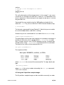
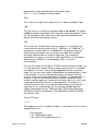
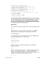
Team TOSCA: left to right, Timmy Ramirez-Cuesta, Stewart Parker (Instrument
Scientists) and John Tomkinson (Group Leader, Molecular Spectroscopy Group).
1 TOSCA
1.1 Description of the instrument and basic INS theory
TOSCA is an inelastic neutron scattering (INS) spectrometer optimised for
vibrational spectroscopy. TOSCA has replaced the previous spectrometers TFXA
and TOSCA-1, however, it retains the advantages of the earlier instruments (ease of
operation and reliability) but simultaneously offers improved sensitivity and
resolution.
TOSCA is a collaborative project between the Consiglio Nationale Recherche (CNR)
of Italy, the Department of Physics at the University of Kent at Canterbury (UK) and
ISIS. (For a detailed list of the participants see the TOSCA website
http://www.isis.rl.ac.uk/molecularspectroscopy/tosca/ and the CNR website:
http://www.ifac.cnr.it/tosca/tosca-main.htm). TOSCA was installed in two phases:
phase 1 was completed in May 1998 and consisted of the backscattering
spectrometer at 12 m, phase 2 added detectors in forward scattering and moved the
spectrometer to 17.0 m. This was completed in September 2000. The move to 17 m
from 12 m has resulted in a large improvement in resolution.
TOSCA User Guide
3 / 66
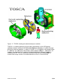
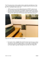
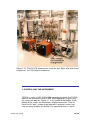
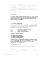
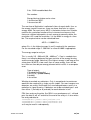
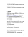
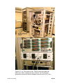
Figure 1.1. TOSCA showing the detector/analyser modules.
TOSCA is an indirect geometry time-of-flight spectrometer at the ISIS pulsed
spallation neutron source at the Rutherford Appleton Laboratory. A section through
one of the analyser modules is shown in Figure 1.2. It is optimal in the energy range
0 - 4000 cm-1 (0 - 500 meV) with the best results below 2,000 cm-1, (250 meV). To
suppress the &gamma-flash and fast neutron background a Nimonic chopper is
installed at 9.5 m. This has a tailcutter (a sheet of B4C) on the leading edge to
remove low energy neutrons that would otherwise result in frame overlap.
TOSCA User Guide
4 / 66
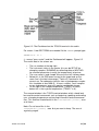
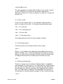
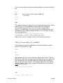
Figure 1.2. A section through one of the analyser modules of TOSCA.
The source of neutrons on TOSCA is the white beam from the water moderator. The
time-of-flight technique is used for energy analysis of the scattered neutrons. A small
fraction of the incident neutrons are inelastically scattered by the sample; those that
are backscattered through an angle of 45° or 135° impinge on a graphite crystal.
Bragg's law states:
λ = 2 d sinθ
(1)
where d (Å) is the interplanar distance in the crystal, λ (Å) is the wavelength of the
scattered neutron and θ is the angle of incidence on the crystal.
From equation (1), since both d and θ are constant only one wavelength (and its
higher orders, λ/2, λ/3 etc...) will be Bragg scattered by the crystal, the remainder will
pass through the graphite crystal to be absorbed by the shielding. The neutrons at
multiples of the fundamental wavelength are scattered by the beryllium filter which
acts as a longpass filter and the remaining neutrons are then detected by the 3He
filled detector tubes. The net effect of the combination of the graphite crystal and
beryllium filter is to act as a narrow bandpass filter.
The energy transferred to the sample, Etrans, is:
TOSCA User Guide
5 / 66
(2)
Etrans.= Ei. - Ef
where Ei and Ef, are the incident and final energies respectively. The kinetic energy,
E, of a neutron is given by:
(3)
where m is the mass of the neutron and v is its velocity. Rearranging (3) gives:
(4)
and since
(5)
travel time = distance / velocity
It follows that the time of arrival at the detector, T, is the sum of the time from the
moderator to the sample, ti, and the time around the analyser, tf, thus:
(6)
Now since the final energy, Ef, the distance round the analyser system, l, and the
length of the flight path from the moderator to the sample, L, are all known, it follows
that the time of arrival at the detector uniquely defines the incident energy, Ei. and
hence the energy transfer at the sample, Etrans. Thus it is a simple matter to convert
from time-of-flight to energy. The result is a spectrometer with no moving parts than
can record spectra from 0 to 8000 cm-1, although the best results are usually
obtained below 2000 cm-1. The resolution of the spectrometer is determined by a
number of factors but for practical purposes can be taken to be 1.25% of the energy
transfer.
The intensity of the ith molecular vibrational transition is proportional to:
(7)
Since neutrons have a mass approximately equal to that of the hydrogen atom, an
inelastic collision results in a significant transfer of momentum, Q (Å-1), as well as
TOSCA User Guide
6 / 66
energy, to the molecule. On TOSCA the design is such that there is only one value
of Q for each energy, (Q2 ≈ ETrans /16 ). (Other instruments at the ISIS Facility and
the ILL allow both the energy and the momentum transfer to be varied, but they
constitute a different story). Ui is the amplitude of vibration of the atoms undergoing
the particular mode. The exponential term in equation (7) is known as the DebyeWaller factor, UTotal is the mean square displacement of the molecule and its
magnitude is in part determined by the thermal motion of the molecule. This can be
reduced by cooling the sample and so spectra are typically recorded below 50K.
σ is the inelastic neutron scattering cross-section of all the atoms involved in the
mode. The scattering cross-sections are a characteristic of each element and do not
depend on the chemical environment. The cross-section for hydrogen is ~ 80 barns
while that for virtually all other elements is less than 5 barns. This means that modes
that involve significant hydrogen displacement will dominate the spectrum. This
dependence on the cross section is why the INS spectrum is so different from
infrared and Raman spectroscopies. There, the intensity derives from changes in the
electronic properties of the molecule that occur as the vibration is executed, (the
dipole moment and the polarisability for infrared and Raman spectroscopy
respectively).
Analysis of INS spectra can be carried out in many ways. For molecular systems,
normal coordinate analysis using the Wilson GF matrix method as implemented in
CLIMAX has long been used. More recently, ab initio methods have proven to be
very successful. The programme aCLIMAX uses the atomic displacements
generated by ab initio packages such as GAUSSIAN98 and DMOL3 to generate the
INS spectrum. See Further Reading at the end of this section for more details on
CLIMAX and aCLIMAX.
A consequence of the indirect geometry is that for energy transfers >100 cm-1 the
momentum transfer vector is essentially parallel to the incident beam. The
significance is that for an INS transition to be observable there must be a component
of motion parallel to the momentum transfer vector. This means that with oriented
samples (such as single crystals or aligned polymers) measurements directly
analogous to optical polarisation experiments carried out .
In addition to the inelastic detectors there are also two 3He filled detector tubes
either side of the incident beam (scattering angle ≈ 179º). These are for elastically
scattered neutrons and enable modest resolution, ∆ d/d ≈ 3 x l0-3, diffraction patterns
to be recorded simultaneously with the inelastic spectrum. It is planned to install two
further banks of diffraction detectors at 45 and 135º. The purpose of the detectors is
to provide a check on the crystal phase of the material and to monitor phase
changes as an experimental variable is changed e.g. temperature and pressure.
There is also a low efficiency scintillation detector (the monitor) in the main beam
just before the cryostat vacuum tank. This measures the incident flux distribution as
a function of time and is used to normalise the spectra.
Further reading
TOSCA User Guide
7 / 66
There is more information about TFXA and TOSCA at the Molecular Spectroscopy
website: http://www.isis.rl.ac.uk/MolecularSpectroscopy/. This includes a list of
publications resulting from work on TFXA and TOSCA. There is also a database of
INS spectra that have been obtained on the instruments. Two types of ASCII and
two types of image files are available for downloading. The database is at:
http://www.isis.rl.ac.uk/INSdatabase/
D. Colognesi, M. Celli, F. Cilloco, R. J. Newport, S. F. Parker, V. Rossi-Albertini, F.
Sacchetti, J. Tomkinson and M. Zoppi.
TOSCA neutron spectrometer; the final configuration,
Appl. Phys. A 74 [Suppl.] (2002) S64-S66.
A description of the current version of TOSCA.
S. F. Parker, C. J. Carlile, T. Pike, J. Tomkinson, R. J. Newport, C. Andreani, F. P.
Ricci, F. Sachetti and M. Zoppi,
TOSCA: A World Class Inelastic Neutron Spectrometer
Physica B 241-243 (1998) 154-156.
This paper gives an overview of TOSCA.
S F Parker,
Vibrational Spectroscopy With Neutrons
Spectroscopy Europe 6 (1994) 14-20.
This gives a brief description of TFXA and highlights some of the areas of research
on the instrument.
J Tomkinson
The Vibrations of Hydrogen Bonds
Spectrochimica Acta, 48A (1992) 329-348.
Illustrates the application of INS to hydrogen bonding studies.
G J Kearley,
A Review of the Analysis of Molecular Vibrations Using INS
Nuclear Instruments and Methods in Physics Research, 354 (1995) 53-58.
An excellent overview of how to analyse INS data using normal coordinate analysis.
J Tomkinson
Neutron Molecular Spectroscopy
in Recent Experimental and Computational Advances in Molecular Spectroscopy,
(R Fausto ed.) Kluwer, 1993 pp229-249.
Briefly describes the theory of INS (and references to in-depth treatments) and some
applications.
aCLIMAX is available from http://www.isis.rl.ac.uk/molecularspectroscopy/
It is described in:
D. J. Champion, J. Tomkinson and G. J. Kearley
a-CLIMAX: a new INS analysis tool
Appl. Phys. A 74 [Suppl.] (2002) S1302-S1304
and
A. J. Ramirez-Cuesta
TOSCA User Guide
8 / 66
aCLIMAX 4.0, The new version of the software for analysing and interpreting INS
spectra
Computer Physics Communications, in press 2003.
B. S. Hudson
Inelastic neutron scattering: a tool in molecular vibrational spectroscopy and a test of
ab initio methods
J. Phys. Chem. A, 105 (2001) 3949-3960.
A demonstration of the power of the combination of ab initio calculations and INS
spectroscopy.
1.2 Sample Environment on TOSCA
The beam size at the sample position is 40 mm high by 40 mm wide. It is clearly
advantageous to fill as much of the beam as possible. For the best resolution the
sample should be 1 mm thick, however, samples up to 4 mm thick are usable.
Solid samples are usually just wrapped in aluminium foil and attached to a
centrestick (see section 2.2 Preparing samples). Liquid samples are run in thin
walled aluminium cans. Air or moisture sensitive samples (solid or liquid) should be
loaded into the cans in a glovebox.
As explained in the previous section, to maximise the INS intensity it is necessary to
reduce the Debye-Waller factor as much as possible, thus virtually all samples on
TOSCA are cooled. Cooling below 50K makes little difference to the spectrum, thus
a Closed Cycle Refrigerator (CCR) which attains temperatures below 20K region is
adequate for most samples, see Figure 1.3. This has the virtues of being reliable,
cheap to run and simple to operate. The CCR is isolated from where the sample sits
and uses helium exchange gas to cool the sample. This has the advantage that the
sample can be changed without warming the CCR, thus samples can be changed in
a matter of minutes without difficulty (see section 2.5 Changing a sample).
The TOSCA CCR has a an internal diameter of 100 mm so will take standard ISIS
centresticks. In addition, there are a number of dedicated centresticks for special
applications. The most important of these is the 24 position automatic
samplechanger. This is described in detail in section 2.4 and 3.5.
If temperatures below the base temperature of the CCR (~ 20K) are required then
normal ISIS practice would be to replace the CCR with a liquid helium cryostat
("orange cryostat"). Because of space constraints this is not possible on TOSCA.
Instead, there is a centrestick that incorporates a liquid helium bin in its shaft. The
design is such that it holds sufficient liquid helium to enable a spectrum to be
TOSCA User Guide
9 / 66
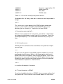
recorded, see Figure 1.3. It may also be pumped on to give a base temperature of ~
1.5K. It is available for use but must be requested well in advance of the experiment
(a minimum of two weeks and ideally on the proposal form).
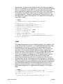
Figure 1.3: The liquid helium centrestick for use on TOSCA
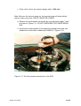
For pressure experiments there are two options. For pressures up to 4 kbar, the
helium intensifier should be used. This allows relatively large samples (the can is 7
mm diameter x 40 mm long) to be used and the pressure can be adjusted with the
centrestick in the beam. For higher pressures, the McWhan clamped cell is used.
The McWhan cell, see Figure 1.4, uses pre-stressed alumina inserts to achieve
pressures of up to 25 kbar. The sample sizes are of the order of 4 mm in diameter
and 10 mm long. It is not possible to pressurise in-situ, and it takes several hours to
cool the whole cell once it is on the instrument. If experiments at pressure are
intended then the equipment must be requested on the proposal form. It is not
available on demand.
TOSCA User Guide
10 / 66
Figure 1.4: A McWhan cell for pressure experiments up to 25 kbar.
2. SAMPLE HANDLING
This section describes how to prepare a sample, load it into TOSCA and what to do
if a centrestick gets stuck in the instrument.
2.1 Safety
There are a number of safety issues associated with work at ISIS. The most obvious
is the radiation hazard from the neutron beam and from irradiated samples and
sample environment equipment. This is minimised by the use of interlocks,
monitoring the radiation levels and appropriate handling and storage of irradiated
materials. If in doubt, ask (your local contact, Health Physics or the Main Control
Room). Before you start an experiment you must watch the ISIS safety video (in
either the DAC or the coffee room in R3) and sign the yellow card. There is also the
risk of exposure to chemicals, in this case the handling instructions on the back of
the sample sheet state the required procedures to follow. Note that cadmium metal
is toxic (it also activates in the beam) so should be handled with care. On removal
from a cryostat, samples and centresticks are usually very cold, so should not be
handled without gloves. Some of the sample environment equipment is heavy or
bulky, so should be carried with due respect.
2.2 Preparing samples
The laboratory’s official handling instructions will be found on the back of the sample
requirement form. You are required to observe them. For solids the easiest way to
present the sample is to load it into an aluminium foil sachet. These are constructed
as described in section 2.2.1. For liquids, a thin walled aluminium can is used. The
same containers can be used for air or moisture sensitive samples, except that the
can is loaded in a glovebox.
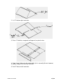
2.2.1 Preparing an aluminium sachet
1. Tear off a piece of foil 20 cm long and fold it over
TOSCA User Guide
11 / 66
2. 1st ‘Z’ fold on right-hand side
3. Press ‘Z’ fold flat, using back of fingernail, or plastic ruler.
4. From "outer" fold mark off sachet width (this is normally 40 mm; however,
for bulky samples this must be ~50 mm).
5. 2nd ‘Z’ fold, on left-hand side
TOSCA User Guide
12 / 66
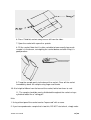
6. Press Z fold flat and cut away excess foil from the sides.
7. Open the sachet with a pencil or spatula.
8. Fill the sachet. Note that it is often valuable to know exactly how much
sample is in the beam, so weighing the sachet before and after filling it is
good practice.
9. Tamp the sample gently to the bare of the sachet. Close off the sachet
immediately above the sample using finger and thumb.
10. At a height of 40mm from the base of the sachet, fold a few times to seal.
11. The sample should be evenly distributed throughout the sachet using a
cylindrical bottle like a "rolling pin".
Hints
1. Using a blunt pencil the sachet can be "impressed" with a name.
2. If you have produced a sample that is too thin, DO NOT start afresh, simply make
TOSCA User Guide
13 / 66
another and run both!
3. If you puncture a sachet, enclose this sachet in some Al foil which can be gripped
on the centrestick as usual.
4. If you are using sachets on the samplechanger, ensure that they will fit within one
of the aluminium frames
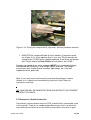
2.2.2 Preparing a liquid cell.
For liquid or air sensitive samples an indium wire-sealed thin-walled aluminium can
should be used. With liquid samples the cell should be filled in a fume hood or a
glovebox if sensitive to the atmosphere. For air or moisture sensitive solids, the
sample should be loaded, and the can assembled, in the glovebox. There are two
types available. One type of cell is designed to go on the 24-position samplechanger
so up to 24 samples can be loaded simultaneously (these can be all cans or a
mixture of sachets and cans). These cans use 1 mm indium wire. Figure 2.3 shows
one of these cells disassembled and a complete cell. The cans have pathlengths of
1, 2, 3 or 5 mm, by suitable choice of the top-plate. For hydrogenous liquids, the 1
mm length should be used since this is sufficient sample to give an excellent
spectrum in around 6 hours. The cells can be used either on the 24-position
samplechanger or clamped to a standard centrestick.
Figure 2.1: A liquid cell for the 24 position samplechanger. Left: baseplate, middle:
top-plate, right: assembled.
Figure 2.2 shows the second ("HET") type cell of thin walled aluminium sample can
and its components. The can consists of two outer cases and a spacer. The spacer
thickness can be varied between 1 and 10 mm. The can is sealed using either
indium wire (narrow grooves) or with Viton O-rings (wide grooves). Since the width of
the can is much greater than that of the beam, solid samples should be loaded into a
TOSCA User Guide
14 / 66
sachet and this positioned in the centre of the can before assembly. To reduce
scattering from the cell, it should be completely shielded with cadmium apart from
the opening at the front of the cell. Owing to the large mass of the cell, once loaded
and attached to the centrestick, it should be immersed in liquid nitrogen for a few
minutes immediately prior to putting the centrestick in the cryostat. This reduces the
cool-down time to less than an hour, from several hours.
Figure 2.2: The components of a liquid cell and an assembled cell, shielded with
cadmium mounted on a centrestick.
2.3 Loading the samples onto a centrestick.
For solid samples in sachets, the simplest method is to attach the sachet to the
aluminium baseplate of an HET type can (lower left in Figure 2.2) with small strips of
aluminium sticky tape. The beam centre is 1165 mm below the underside of the
centrestick flange and the beam itself is 40 x 40 mm (h x w). The sample should
cover as much of the beam area as possible and be preferably no more than 2 mm
thick. If measurements at temperatures other than the base temperature of the CCR
(~12K) are intended, then the best method is to attach heaters and a sensor to the
sides of the plate. Note the sensor number! Care should be taken that only the
sample and the Al sachet are in the beam; items such as sensors, heaters, tape or
wire should not intrude. If it is intended to measure more than four samples at base
temperature it is worth considering using the 24 position samplechanger. For six or
more, its use is almost mandatory. Samplechanger type liquid cells are held by a
clamp attached to the end of the centrestick (see Figure 2.14). HET cans have a
mounting plate with an M8 screw that attaches to the end of the centrestick (top in
Figure 2.2).
2.4 Loading the 24 position samplechanger
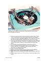
The 24 position samplechanger is shown in Figure 2.3, it consists of two parallel
endless chains connected with horizontal bars from which the samples are
suspended. The device can be controlled either manually from a handset attached to
the control box in the electronics rack next to the services panel or under computer
control. The latter is described in section 3.5. Note that samples can only be run at
TOSCA User Guide
15 / 66
the base temperature of the cryostat (~20K with the samplechanger), it is not
possible to put heaters on the sample or to heat the cryostat. You should also
assume that the samplechanger can only be run forwards, so the samples should be
loaded in the order in which you wish to run them.
Figure 2.3: The 24 position samplechanger in its cradle (right) and its controller
(bottom panel in electronics rack on the left).
The samplechanger can be loaded with sachets or liquid cells in any combination.
Sachets are mounted on an aluminium frame and held on with aluminium sticky
tape. The sachet must be held within the frame it should not protrude above it and
the sticky tape should not be touch the chains. The right-hand side of Figure 2.4
shows a correctly mounted sachet To mount a liquid cell, it may be necessary to
remove an aluminium frame. In either case, note the six digit number on the
clamping plate.
TOSCA User Guide
16 / 66
Figure 2.4: Loading samples on the 24 position samplechanger. Left: empty
aluminium frame for a sachet, note the six digit number at the top of the clamping
plate. Right: sachet mounted on a frame. A liquid cell is mounted at the position
below it.
To move to a vacant position on the samplechanger, use the handset attached to the
controller in the electronics rack, see Figure 2.5. There are four buttons on the
handset: forward is the second from the top, back is the bottom button (the first and
third buttons are not used), press and hold for either direction. There is a green
status light to the right of the digital display on the control rack, the samplechanger
will only move when this illuminated. When the sample is in the correct position,
movement stops and the red "sample in lock" light is illuminated, there are also two
red lights on the samplechanger that show the sample is in the correct position. The
digital display will have changed by ~1600. To install or remove the samplechanger
in TOSCA requires the use of the crane. This must be done by the local contact.
Figure 2.5: The 24 position samplechanger controller
TOSCA User Guide
17 / 66
2.5 Changing sample
Before changing a sample, familiarise yourself with the TOSCA cloche and the area
around it. Figure 2.6 shows the gate and interlocks to the TOSCA enclosure and
highlights the location of the important items. The following procedure assumes that
the four-position sample changer is being used. If an aluminium can or other large
piece of equipment (e.g. a catalysis cell or a McWhan cell) is being used, then it is
essential to pre-cool this in liquid nitrogen immediately before insertion into the
cryostat, otherwise the cool-down time is prohibitively long. If the sample is precooled in liquid nitrogen, then ensure that the lowest baffle does not come into
contact with the liquid nitrogen because it can freeze in the cryostat and cause the
centrestick to become stuck.
TOSCA User Guide
18 / 66
Figure 2.6: The TOSCA cloche and services panel showing the interlocks interlocks,
pump and He flow control.
Access to the TOSCA CCR is via the "cloche" located on the mezzanine floor. This
is interlocked by the standard ISIS key system. The interlocks on the instruments are
there to try to make it impossible to get close to the neutron beam. There are two
sets of interlock keys: The Master (‘M’) key, which is to be found on the front of the
Green box and is labelled with a red tag; The remainder are ‘S’ keys which are
located in the Blue box, see Figure 2.7. There are two shutter control boxes: one in
the cabin and one on the services panel behind the cloche.
Note: You only have control of the shutter if the Master key is in the Green box. If
you try to operate the shutter whilst the interlocks are not complete you will trip-off
ISIS.
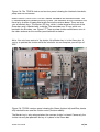
Figure 2.6: TOSCA services panel showing the Green (bottom left) and Blue (centre
left) interlock boxes and the shutter control (bottom middle).
The Master key is only released when the neutron shutter is closed. Conversely the
shutter can only be opened if the key is in place in the Green box.
TOSCA User Guide
19 / 66
The ‘S’ keys give access to the sample enclosure and other controlled areas. They
can be released by placing the Master key in the bottom right hand slot of the Blue
box. This is normally the only vacant slot.
"END" the current run (the Dashboard changes to "SETUP") and write: the
time, Run No and total number of microamps used into the Instrument Diary.
2. Close the shutter to the beam (green button marked "CLOSE" on the Neutron
Beam Shutter Control Panel located on the services panel by TOSCA, Figure
2.7, and in the cabin Figure 2.8. The shutter takes a few minutes to close.
1.
Figure 2.8: The shutter controls in the TOSCA cabin.
3.
Ensure the shutter is closed. Wait until both the blue fluorescent light, and the
red "Beam On" sign are off and the green "CLOSED" light is illuminated in the
shutter control panel. The radiation monitor on the wall of the target station
must show a green light and a reading of less than 20 µ Sv/hr, Figure 2.9.
TOSCA User Guide
20 / 66
Figure 2.9: The radiation monitor on the target station wall. TOSCA's is
labelled "N8 TFXA" (upper right).
3.
4.
5.
6.
7.
8.
9.
10.
Turn anti-clockwise the "Red" (i.e. carrying a red tag) key in the
"Green" box and release it.
Engage the Red key in the "Blue" box, and turn it clockwise.
This liberates all other keys in the Blue box. Select any other key and
turn it anti-clockwise and remove it.
Remove the shielding from the top of the cloche.
Place the key in the enclosure lock and turn it anti-clockwise.
Rotate the bolt fully and withdraw. the bolt fully and withdraw.
Open fully the small brass valve on the flowmeter to the helium cylinder
(see Figure 2.6). Do not adjust the regulator, the gas pressure on the
gauge should read about 0.5 bar.
Open valve No's 1, 2 and 4 on the cryostat pump (see Figure 2.10) The
vacuum gauges should show the pressure rising slowly, meanwhile the
He gas flow is at maximum. Ensure that the light blue valve on the
CCR is pointing vertically, Figure 2.13.
TOSCA User Guide
21 / 66
Figure 2.10: The pump manifold and sketch showing the numbering of the
valves.
TOSCA User Guide
22 / 66
11.
Close valve 2 when the vacuum gauge shows 1000 mbar.
Note: Because the vacuum gauge on the cryostat pump will automatically
release excess pressure: VALVE 4 MUST BE CLOSED.
12.
Remove the thermometer connection by unscrewing the upper "silver"
knurled nut, Figure 2.11. DO NOT UNSCREW THE LOWER BRASS
NUT.
13.
Unscrew the retaining bolts at the top of the sample centrestick and
withdraw the centrestick smoothly but RAPIDLY. (Figure 2.12).
Figure 2.11: The thermometer connection on the CCR.
TOSCA User Guide
23 / 66
Figure 2.12: Illustrating centrestick withdrawal
TOSCA User Guide
24 / 66
Figure 2.13: Photo graph of the cryostat with the centrestick withdrawn and
blanking flange in place. The blue valve on the side of the CCR and the
pressure gauge are labelled.
14.
15.
16.
17.
18.
19.
20.
21.
22.
Cover the cryostat top with the blanking plate and bolt it down (Figure
2.13). If it will be more than a few minutes before the next sample is
inserted, the helium should be pumped out, see 19 and 20. This keeps
the cryostat cold and reduces cool-down time for the next sample.
Take the centrestick to the work bench and replace the old sample with
new sample (see Section 2.2 and 2.6). If a different centrestick is to be
used, ensure that the sample is inside the lead castle on the work
bench.
Unscrew bolts retaining blanking plate, the pressure falls to 0.
Remove the blanking plate and push the centrestick down into the
cryostat, RAPIDITY is needed but CARE must be used. Bent
centresticks are expensive to replace.
Secure centrestick lid with bolts.
Switch on the cryostat pump (switch on right hand side of pump).
Open valves 2 and 3, vacuum gauge begins to register.
WAIT until the pressure drops to 25 millibar on the gauge on top of the
CCR.
Close the blue valve on the CCR and valves 2 and 3 and switch off the
pump.
TOSCA User Guide
25 / 66
Reconnect the thermometer cable to centrestick.
Check which sample is oriented correctly (usually perpendicularly) with
respect to the neutron beam.
25. Close the interlocked door (do steps 4 - 8 in reverse.)
26. Open the shutter and start collecting data (see section 4: Controlling
the instrument).
23.
24.
2.6 Removal from centrestick
This work should be done with the sample centrestick being on the TOSCA
centrestick stand, on the work bench on the mezzanine floor.
Turn the hot air blower on and warm the sample.
Release the sample sachet from the cadmium lantern using long-nose
pliers to remove the retaining wire or aluminium tape. Remember that
cadmium metal strongly activates in the neutron beam.
29. Remove the sample using tweezers - or - if you must, gloved hands.
27.
28.
NEVER HANDLE ACTIVE SAMPLES WITH BARE HANDS.
TOSCA User Guide
26 / 66
Figure 2.14: Testing the sample with β (top) and γ (bottom) radiation monitors.
4.
MONITOR the sample with both β and γ monitors (β monitor cap off,
see Figure 2.14). If the radiation level is less than 75 µSv consign the
sample to the TOSCA active sample cupboard. If the levels are greater
than 75 µSv inform the Duty Officer for instructions (ext: 6789)
Samples consigned to the active cupboard MUST be in sealed plastic bags
and labelled with the owner's and sample names and date. The sample
environment form should also be included. Spare bags are in the tool
cupboard and the prep. labs.
Note: If you really must transfer active loose powders between sample
holders or if a sachet bursts accidentally, phone the Duty Officer for
instructions and help.
NO SAMPLES MAY BE REMOVED FROM ISIS WITHOUT THE CONSENT
OF HEALTH PHYSICS.
2.7 Removal of a Stuck Centrestick
Occasionally, during removal from the CCR a centrestick is found to be stuck
in the cryostat. There are a number of possible causes of this, of which the
most common are failure to ensure that the centrestick is dry when it goes
TOSCA User Guide
27 / 66
into the cryostat, a leak around the top flange of the centrestick caused by the
flange being incorrectly seated on the O-ring, or if the sample was pre-cooled
in liquid nitrogen, solid nitrogen gluing the lowest baffle to the cryostat wall. By
whatever means, the usual result is a small amount of air or nitrogen
condensing between the baffles of the centrestick and the cryostat wall. In
these cases, warming the cryostat to 90K is sufficient to free the centrestick. If
ice is present, then it is necessary to warm it to near room temperature.
THE FIRST ACTION SHOULD BE TO INFORM YOUR LOCAL CONTACT.
The sequence of actions is:
5.
6.
7.
8.
9.
10.
11.
Fill the centrestick chamber with helium gas. The flange of the
centrestick must be bolted down.
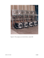
Switch off the two CCR compressors labelled TOSCA on the ground
floor by the outer wall of R55 inside the hall, Figure 2.15. DO NOT
TOUCH the five compressors that are outside the hall, Figure 5.2.
Warm the cryostat to 90K.
When the sample temperature is 90K attempt to remove the
centrestick as normal (see section 2.5)
If the centrestick cannot be removed, wait until the cryostat has
reached room temperature.
When the centrestick has been removed, replace the blanking flange
and flush the sample volume with helium gas three times before
installing the next sample.
Re-start the CCR compressors.
TOSCA User Guide
28 / 66
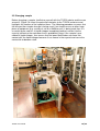
Figure 2.15: TOSCA CCR compressors inside the hall. Right: 40K cold shield
compressor, left: 20K sample compressor.
3. CONTROLLING THE INSTRUMENT
TOSCA is run by a DEC-ALPHA 500 computer located in the TOSCA
cabin on the mezzanine level of R55. After logging-on (if necessary)
the screen will look like Figure 3.1. In the centre of the toolbar at the
bottom of the screen are four buttons labelled one to four. Each of
these has its "own" screen associated with it and each screen can
have as many windows as desired. The convention that is used is:
TOSCA User Guide
29 / 66
Screen 1 is used for displaying the instrument status (the
"Dashboard") and controlling the instrument
Screen 2 is used to display data using GENIE
Screen 3 is for OPENGENIE
Screen 4 is for the users e.g. to telnet to their home computer.
To create a window, on the toolbar click on the icon for a terminal (4th
from the left in Figure 3.1), a menu then pops-up and click on the item
labelled DECTERM. This procedure is the same in any of the screens.
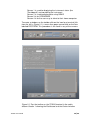
Figure 3.1:Top: the toolbar on the TOSCA terminal in the cabin,
bottom: Screen 1 showing the Dashboard and the Control window.
TOSCA User Guide
30 / 66
Figure 3.2: The Dashboard on the TOSCA terminal in the cabin.
For screen 1 two DECTERMs are needed. At the TOSCA> prompt type:
TOSCA>stat on ←
(← means "press enter") and the Dashboard will appear, Figure 3.2.
The useful data in the screen are:
The run number at the top right.
The instrument status in the centre, this can be SETUP for
changing samples, RUNNING for collecting data or WAITING
for a control parameter (usually the temperature) to be true.
The user name(s) and sample title are at the left, halfway down.
Below this is the ISIS beam current to the target and on the
same line is the total microamps ("Total uA") received in the
current run. For adequate statistics from a hydrogenous sample
this should be at least 600 (3 - 4 hours runtime), small samples
or non-hydrogenous ones will require considerably longer.
On the right is the sample temperature ("TEMP") in Kelvin,
below this is the cryostat temperature ("TEMP1" in K).
The second window is the TOSCA control window, which should only
be used for control commands such as beginning, updating and ending
runs, changing temperature and starting instrument control command
files. This terminal should be left in the tosca$disk0:[tosca] area
at all times.
Note: Do not leave files in the
tosca$disk0:[tosca] area that you want to keep. The area is
regularly purged.
TOSCA User Guide
31 / 66
3.1 Change
The change command allows the user to edit the Dashboard
information. Typing the command
TOSCA> change ← (can be abbreviated to cha)
will initiate the Dashboard editor. Move between areas using the up
and down cursor keys and over type. There are six pages, you will only
modify the first. This page contains title and user information. When
entering the title please be informative; abbreviations or sample
numbers are not helpful. The accumulated spectra on TOSCA form a
unique library whose usefulness is compromised if the spectra are not
clearly identified.
To exit press [PF1] (found on the numeric keypad on the right of the
keyboard). A prompt will appear at the top of the screen, to exit press
[e].
3.2 Setting sample environment parameters
The top right hand portion of the Dashboard displays the sample
environment parameters sample temperature (normally TEMP) and
cryostat temperature (normally TEMP1). If you have changed
centresticks or are using a sensor attached to the sample rather than
the one built into the centrestick, you will need to input the sensor
number. Each sensor is individually calibrated and a unique four digit
number is written on the sensor. On each centrestick is a label with
"SEN" on it that gives the sensor number. To check the censor number
type:
TOSCA> cshow temp/full (or temp1)
The computer will respond:
The "Device number" is the sensor number. To input a different sensor
number type:
TOSCA User Guide
32 / 66
TOSCA> cset temp/devspc=xxxx
Where xxxx is the sensor number.
Most spectra are recorded at the base temperature of the cryostat. If
other temperatures are required, then cartridge heaters need to be
attached to the sample before it is loaded into the cryostat. To change
the sample temperature the cset command is used as follows:
TOSCA> cset temp/value=1OO/control
will set the sample temperature to 100K
Limits can be set to ensure that data are only collected between
specified temperatures:
TOSCA> cset
temp/value=45/lolimit=40/hilimit=50/control
will ensure that data is only collected while the sample temperature lies
between 40K and 50K. If the sample temperature strays out of these
limits the instrument will be put into "WAITING" mode.
If run control is no longer required the nocontrol qualifier should be
used:
TOSCA> cset temp/nocontrol
When measurements are to be made at base temperature, the heater
is usually switched off. If you want to warm up the sample, and there
appears to be no response to the cset temp command, check that the
heater is plugged in and switched on. In the TOSCA cloche, the heavy
black cable must be plugged into the socket marked "HTR" on the
same black box to which the temperature sensor lead is attached. The
heater on/off switch is on the Eurotherm crate, in the electronics rack in
the TOSCA cabin. The % of the maximum power is also controllable.
To determine the current setting type:
FEM> cshow max_power/enq
The computer will return:
Value returned was xx
Where xx is the % power. To change this value type:
FEM> cset max_power ??
Where ?? is the desired value (0 ≤ ?? ≤ 100)
TOSCA User Guide
33 / 66
3.3 Data collection commands
All the following instrument control commands may be abbreviated to
three letters.
begin
update
store
pause
resume
abort
end
Starts a run.
Stores the data collected so far in the current run parameter table
(CRPT)
Stores the data collected up to the last update in the file
tosca$disk0:[tfxmgr.data]TSCA0<xxxx>.sav. The store
command should always be preceded by an update
Pauses data collection.
Resumes data collection.
Aborts the current run without saving any data.
Ends the current run and stores the data in
TOSCA$disk0:[tfxmgr.data]TSC0<xxxx>.raw The data is
analysed automatically by a batch program when a run is ended. This
process takes a few minutes, after that it can be viewed using GENIE.
3.4 Using command files
Command files are written to control the instrument. An example is:
$ begin
begins run
$ waitfor 1000 uamps
waitfor1000 m Amps
$ end
end run
$ cset
temp/value=80/lolimit=75/hilimit=85/control sets temperature limits
wait 40 mins
$ wait 00:40:00
(temperature
stabilisation)
$ change title """Sample at 80K"""
title change (triple "are
essential)
$ begin
begins run
$ waitfor 1000 uamps
$ end
$ exit
spaces are essential
Command files are created using the VMS editor and end with the
extension .com.
TOSCA User Guide
34 / 66
They are run from the TOSCA Control window using @< filename>. To
interrupt a command file type [Control] Y. Note that you are unable to
use the window when a com file is running.
Note: The two commands WAIT and WAITFOR are different, and
confusion over their use is one of the main causes of command file
failures.
WAIT
This is a VMS command that waits for a specified time. The time must
be given in the hrs:mm:secs format used by the VMS operating system
e.g.
WAIT 01:30:00
will wait for one hour 30 minutes before executing the next command.
WAITFOR
This is an instrument control command and can be used to wait for
certain amount of data to be collected. The most common usage of the
command is to wait for a certain number of microamps, in this case the
suffix uamps must be given after the number e.g..
waitfor 1000 uamps
will wait for 1000 microamps of beam current before executing the next
command. If ISIS goes off then it will sit and wait! Note that the format
is rigid, there must be a space between the number and "uamps".
A common requirement is to wait until the sample reaches a given
temperature. This can usually be estimated fairly accurately and a
command file with a WAIT statement used. Alternatively, the cset
command with the /control option can be used, but data is not
collected while in the WAITING state. Instead, if the /chklog option
is used with cset then the next command is only executed when the
condition is true.
A sample command file is:
$ cset temp/value=20/lolimit=5/hilimit=25 sets
temperature limits
$ begin
$ cset temp/chklog
waits until the temperature is in the range 5 - 25K
$ end
TOSCA User Guide
35 / 66
end run
$ change title """Sample at 20K"""
$ begin
begins new run
$ exit
This will collect data until the temperature is in the range 5 - 25K, when
it ends the run, changes title and starts a new run. The commonest use
for this command is while waiting for the sample to cool, but it is not the
only possible use.
Command files are created using the VMS editor and end with the
extension .com. They are run from the TOSCA Control window using:
@ <filename>
To interrupt a command file type [Control] Y. Note that you are unable
to use the window when a com file is running.
A better way to run a command file is to submit it toTOSCA$BATCH by:
submit/que=tosca$batch ←
The advantages are that your local contact can interrupt it and modify it
remotely if necessary, this is not possible if @ <filename> is used.
Also, in theory at least, if the TOSCA computer crashes, the batch job
should restart, using @ <filename>, the command file is terminated.
To check on the status of the command file use:
sho que tosca$batch ←
The response will be:
where Jobname is the name of the command file. To stop a batch job
type:
del/entry=xxxx ←
where xxxx is the entry number returned by the sho que command,
1767 in this instance.
3.5 Using the 24 position samplechanger
The 24 position samplechanger can be used either manually or under
TOSCA User Guide
36 / 66
computer control. In both cases the initial setting-up procedure is the
same. The samples are arranged on an endless chain and the can at
the top of the samplechanger is viewed through the Perspex window
(DO NOT CLEAN WITH SOLVENT!) by a webcam. The samples are
tracked by the numbers on the clamping plate. This consists of six
digits, a four digit number and a two digit checksum. Thus in Figure 2.4
the number 003205 is visible, so this is: 0032 and (0 + 0 + 3 + 2 = 05).
When a sample is in the beam, the can number is not visible but its
counterpart 12 positions away is visible. Thus the first operation after
loading the samples onto the samplechanger, see section 2.4, is to
create a table of sample, can number and can number at the top when
the sample is in the beam. An example is:
Can
2507
2810
2103
1203
505
1405
202
2709
1506
2406
2911
808
707
3609
303
404
3508
3306
1910
3003
2204
101
2002
2608
Top
707
3609
303
404
3508
3306
1910
3003
2204
101
2002
2608
2507
2810
2103
1203
505
1405
202
2709
1506
2406
2911
808
Sample
0.5 mm cell H2O
1 mm cell H2O
2 mm cell H2O
Ti/NaAlH4 (fresh)
Ti/NaAlH4 (after TPD)
Ti/NaAlH4 (after 10 bar H2)
Ti/NaAlH4 (after 100 bar H2)
Sn/NaAlH4 (fresh)
Sn/NaAlH4 (after TPD)
Sn/NaAlH4 (after 10 bar H2)
Sn/NaAlH4 (after 100 bar H2)
n-propanol
Note that not all the positions need to be filled, but pairs of cans must
both have numbers.
After creating the table, the cables are removed and the
samplechanger is then loaded into TOSCA using the crane, this must
be done by the local contact. (Note: the samplechanger must be
bolted down before evacuating the IVC). After installation, the main
control cable, the Ethernet cable and the power supply for the webcam
and the thermometer cable are reconnected. Figure 3.3 shows the
samplechanger installed in TOSCA and the important points
TOSCA User Guide
37 / 66
highlighted.
Figure 3.3: The samplechanger installed in TOSCA.
Before setting the interlocks it is wise to check that everything is
working! The lights immediately below the webcam should be on and
the "sample in lock" light on the controller, Figure 2.5, and on the
samplechanger, (indicated on the right-hand side of Figure 3.3), should
be illuminated. The webcam should also be working. This can be
viewed in the TOSCA cabin using the Ray-of-Light programme on the
PC next to the VMS screen (see later) or at: http://eye2.nd.rl.ac.uk/java
on the general use PC. (It should be listed under Favourites in Internet
Explorer).
The chain of command is: VMS → Ray-of-Light → controller →
samplechanger. The samplechanger can be operated from any point
along the chain, although full automation is only possible from VMS.
The Ray-of-Light interface is shown in Figure 3.4.
TOSCA User Guide
38 / 66
Figure 3.4: The Ray-of-Light interface.
When the control system for the samplechanger was designed it was
intended that it would be run exclusively from the Ray-of-Light interface
(a GUI on top of the LabView control programme). Ultimately, this will
happen when TOSCA is run from a PC rather than VMS. In practice, it
is better to run the samplechanger from VMS and use Ray-of-Light
simply as a connection in the chain. However, for the VMS commands
to work, Ray-of-Light must be operating correctly. When the main
supply cable is detached from the samplechanger Ray-of-Light will
often hang. This is noticeable because the webcam view is not correct.
It is re-started by pressing "QUIT" in the top left of the screen, the
programme will exit and automatically re-start. This takes a couple of
minutes.
The samplechanger can be moved by using the buttons in the lower
centre of the screen. If you change the number of steps (=positions),
labelled #Steps, then reset it to 1 afterwards because VMS uses the
value set on the screen.
In theory, going forwards or backwards should work equally well.
Experience shows that going backwards is when the samplechanger is
most likely to jam, the only cure is to remove it from TOSCA, warm it to
room temperature and put it back in the instrument. This can result in
anything up to 12 hours lost time. You have been warned!
TOSCA User Guide
39 / 66
The samplechanger is run from VMS at the command level (where,
END, BEGIN etc… are done), not in GENIE. The commands are:
next_sample
moves forward number of samples set in "#Steps"
prev_sample
moves back number of samples set in "#Steps"
prev_sample is not recommended as explained earlier. To ensure
reproducible positioning, it moves back two positions, then forward one
so that the limit switches on the samplechanger are always struck from
the same direction. The commands are treated the same as any other
VMS command, so can be included in a command file as usual.
4. DATA ANALYSIS AND VISUALISATION.
Several programs and utilities exist to help you analyse your data
including the GAUS least squares fitting program. TOSCA is unusual in
that for most cases the output from the automatic analysis program is
all that is required. However, if desired, the raw time-of-flight data can
be analysed independently. If you are doing data analysis in your own
directory make sure that you are using the TOSCA GENIEINIT .COM.
Please do not log onto TOSCA and start GENIE as this seriously slows
the system; use a different computer instead e.g. ISISA.
4.1 GENIE
GENIE is the language used at ISIS for data manipulation. A full
description of which, is available in the PUNCH user manual, a copy of
which resides in the TOSCA cabin. Additional copies may be obtained
from the computer support office.
If you are in the TOSCA cabin the GENIE window on screen two
should already be opened. If there is no GENIE window or if GENIE
crashes (rare but not unknown!) it is (re)started by typing "GENIE"
(upper or lower case are both OK since VMS is case insensitive) in a
DECTERM window (see section 3 and Figure 3.1 for how to start a
window). This will create an additional window that can be re-sized
using the mouse. By default GENIE only uses the current screen, it
does not scroll and allow you to use the scroll bar on the right of the
window. This is inconvenient and can be corrected by clicking on the
word "COMMANDS" at the top of the window and selecting the last
item in the list "RESET TERMINAL".
If you are not in the cabin and are attempting to work on TOSCA data
TOSCA User Guide
40 / 66
elsewhere, e.g. in the DAC, the procedure is more complicated and
you should consult your local contact before starting.
When GENIE starts, a page will scroll past which includes each
specialised function available and the command needed to utilise
them. For reference a copy of this can be found in section 7.2. Typing
the command:
sho sym ←
will type the list.
On TOSCA, GENIE is divided into 16 workspaces, w1 – w16. The data
in GENIE is completely volatile and does not alter the original data on
the TOSCA disk. Thus no operation, up to and including crashing
GENIE, will result in loss of data.
4.1.1 Looking at analysed files
For each run, three analysed (i.e. as intensity vs. energy transfer) files
are stored. These are the: the summed back scattering detectors, the
summed forward scattering detectors and the sum of the two sets of
detectors (back + forward). These are called:
trsl
trslba
trslfo
sum of back and forward detectors
backscattering detectors
forward scattering detectors
To read in an analysed file type:
»r wl [tosca.user]trslxxxx.ana ←
»r wl [tosca.user]trslbaxxxx.ana ←
»r wl [tosca.user]trslfoxxxx.ana ←
For the total, back or forward scattering detectors respectively, where
xxxx is the run number. For TOSCA-1 (run numbers 1 - 2134) ) there
are only backscattering spectra, so only the first command is
applicable. For TFXA spectra use:
»r wl [tfxa.user]trslxxxx.ana ←
To display a spectrum (assumed stored in workspace 1) type:
»d wl ←
This will plot the spectrum in the GENIE graphics window. The range of
data displayed may be specified:
TOSCA User Guide
41 / 66
»d wl 50 100 0.1 0.3 ←
This plots workspace 1 between 50 and 100 (x units) and 0.1 and 0.3
(y units). GENIE assumes that the two numbers following the
workspace number are x values; to specify a y range, an x range must
be given first.
4.1.2 Types of plot
As well as the histogram plot, it is also possible to plot the data as
points, line plots or error bars. To change the type of plotting, type:
»d/l ← For a line plot
»d/h ← For a histogram plot
»d/e ← For error bars
»d/m ← For the data points
The display defaults to the last of these options entered.
4.1.3 Overlaying spectra
To overlay spectra one on top of another you can type:
»p w? ←
Where ? is the number of the workspace to be added to the current
graphics window. This is useful for comparing accurately two or more
spectra. A useful device is to display the data using the d command in
a histogram format and then to overlay the error bars by using:
»p/e ←
4.1.4 Binning and rebinning
The bin size represents the number of adjacent points averaged for
each data point. So a binning of 1 (i.e. no binning) has a high accuracy,
but may also have high noise levels. A numerically larger binning will
give reduced noise, but the resolution will be degraded, thus binning
acts as a crude type of smoothing. The advantage is that the data in
the workspace is not permanently changed. To alter the binning, type:
»a b x ←
TOSCA User Guide
42 / 66
Where x (integer only) represents the binning number, usually between
1 and 10.
The GENIE command "rebin" allows different portions of the
workspace to be averaged to different extents (unlike binning which
operates on the whole workspace), but permanently changes the data
in the workspace. Thus the best method is to copy the data to another
workspace by e.g.:
»w1 = w2 ←
and then to experiment on the second workspace. There are two forms
to the command:
»reb w2 16 (2) 4000 ←
»reb w2 16 [.02] 200 [.005] 4000 ←
In form 1 with ( ) brackets the value inside the brackets is in x units. So
for a spectrum in wavenumbers, the first command will rebin the data
into 2 cm-1 intervals between 16 and 4000 cm-1. Rebin truncates to the
limits given. Thus if the upper limit was 2000 cm-1 then the data would
only be retained between 16 and 2000 cm-1. Note that multiple ranges
are possible, as shown in the second example.
In form 2 with [ ] brackets the value inside the brackets is related to the
size of the time bins in the raw time-of-flight data. When the data is
transformed from time-of-flight to energy transfer a value of 0.005 is
used across the entire spectrum. Thus in form 2 the spectrum is being
rebinned in "4’s" (0.02 = 4 x 0.005) between 16 and 200 and in "1’s"
between 200 and 4000 cm-1. This is a particularly useful form of the
command since at low energies there are many more data points than
can be justified by the instrument’s resolution function. Thus the data
can be rebinned to improve the signal-to-noise without degrading the
resolution.
4.1.5 Hard copies
To obtain a hard copy of the current data that is displayed in the
GENIE graphics window, type:
»lpr ←
A list of printers is then given and you are prompted for which printer to
use (See Table 4.1). Just type the printer number and a postscript file
will be automatically created and sent to the nominated printer.
Laser printers
TOSCA User Guide
Location
43 / 66
LASER 0
LASER 1
LASER 2
LASER 17
Computer support office, R3.
Coffee room, R3.
DAC, R55.
TOSCA cabin
Table 4.1: A list of the normally used printer devices.
A procedure that will always work but is somewhat more long-winded is
to type:
»k/h ←
This carries out a screen dump of the GENIE display window and
creates a postscript file called DEC_POSTSCRIPT.DAT, in the
directory you are currently in. To print this file from GENIE:
»j "plaserx dec_postscript.dat" ←
Where x is the number of the laser printer (see table 4.1). Remember
to change the disk/directory name if your file is elsewhere. These files
are purged frequently so it is inadvisable to do too many at any one
time.
4.1.6 Using the cursor
Should you wish to find the exact co-ordinates of a peak for example
you can type:
»c ←
A 'cross-hair' will appear in the GENIE graphics window. This can be
positioned using the mouse. When in the correct place click the left
button and a menu will appear, select the desired option. To exit from
the cursor, it is necessary to choose the "EXIT" option from the menu.
By default, values and text are printed vertically at the cursor position.
For annotation of a plot this is inconvenient, if
»c/h ←
is used then the output is horizontal.
4.1.7 Useful functions in GENIE
As well as the built-in functions of GENIE, there are some routines that
are specific to TOSCA that are useful to know about: For most of the
TOSCA User Guide
44 / 66
programmes, when prompted for a workspace, type:
w? (1 ≤ ? ≤ 16). Exceptions will be noted.
QR4
This is to have a look at the spectrum as it is being recorded. Type:
»qr4 ←
This will result in an analysed spectrum that is not saved. The output
of QR4 is placed in workspace w5. The back scattering detectors are in
w7, the forward in w9 and the sum in w5. Note that workspaces w1 w9 are overwritten during the analysis.
FR4
This is the main TOSCA data analysis program. It is normally only
used if data outside the usual range (2 - 500 meV, 16 - 4000 cm-1) is
required or if saved (.SAV) or co-added files are to be analysed or
when the batch file does not run or when the .ANA file has been
corrupted and the data has to be re-analysed. (For co-adding
sequential runs there is a version of FR4 called SR4, see next topic).
Note that the . RAW file is unchanged by FR4 in any of its
manifestations.
The use of a fixed final energy on TOSCA means that each energy (ω)
is associated with a unique value of momentum transfer Q. A second
consequence is that Q is only weakly dependent on the scattering
angle, thus for the small angles subtended by the detector banks, there
is no variation in Q across the detector bank. This means that the
analysis of the raw time-of-flight data on TOSCA is straightforward. In
essence, it consists of normalising each detector spectrum to the
incident monitor spectrum, conversion to energy transfer (in meV) and
summing the detectors to give a single spectrum. This process is
sufficiently routine that it is carried out automatically by a batch file
each time a run is ended and uses the raw time-of-flight data file
(.RAW) to generate the files TRSLxxx.ANA, TRSLFOxxx.ANA and
TRSLBAxxx.ANA in the directory TOSCA$DISKO:[TOSCA.USER] a
few minutes later.
To run FR4 type:
»fr4 ←
The program asks for a number of inputs. In the order in which they are
required these are:
File extension:
1 for . RAW original data
2 for . SAV files saved during a run
TOSCA User Guide
45 / 66
3 for . SUM co-added data files
Run number.
Energy binning choice and a value:
1 for constant ∆E/E.
2 for constant ∆E.
The raw time-of-flight data is collected in bins of equal width, thus as
the energy transfer increases, there are fewer time bins in a given
energy width. For most cases ∆E/E is the better choice since it better
matches the resolution function of the instrument and ensures that
there are sufficient data points at each energy to correctly define the
resolution. ∆E is not the resolution, it is the width in energy of a time
bin. The required value can be calculated from:
∆E/E ≈ √ 0.0002 Emax
where Emax is the highest energy (in meV) required in the spectrum.
For the standard range 2 - 500 meV a value of 0.005 is appropriate.
The energy range to analyse.
This is usually 3.5 - 500 meV (30 - 4000 cm-1). Care is needed since
there is an interplay between the type and size of the energy binning
and the energy range. Note that if the highest energy is too large or the
value given for ∆E/E is too small, then at some energy, there will be
less than one time bin per energy element which results in a computer
error.
Type of output:
1 for double differential
2 for S(Q,w ) (usual choice)
3 for both
4 for neither
Whether to exclude any detectors. Only in exceptional circumstances
would this be required e.g. single crystal studies. For most samples the
detectors are evenly illuminated, thus excluding detectors results in a
reduction in signal-to-noise. If detectors are to be excluded type 1 and
then either 1 (include) or 0 (exclude) for each detector in turn
FR4 then analyses the data, like QR4 it uses workspaces w1 - w9 and
puts the data in w5, w7 and w9 at the end of the analysis. It also writes
the analysed data to:
tosca$disk0:[tosca.user]trslxxx.ana
tosca$disk0:[tosca.user]trslbaxxx.ana
tosca$disk0:[tosca.user]trslfoxxx.ana
so it may be read in subsequently.
TOSCA User Guide
46 / 66
Thus to analyse data using the standard conditions the series of inputs
are:
1 ←
1←
.005 ←
Value must be in this format, 0.005 will
not work
2 ←
500 ←
2 ←
2 ←
SR4
This program analyses spectra that were collected sequentially and coadds the result. The co-addition is performed before the data is
converted to energy transfer since this results in slightly better
statistics. The operation is the same as for FR4 except that the user is
prompted for the number of spectra and the first run number. It writes
the analysed data to:
tosca$disk0:[tosca.user]tsumslxxx.ana
tosca$disk0:[tosca.user]tsumslbaxxx.ana
tosca$disk0:[tosca.user]tsmslfoxxx.ana
where xxxx is the run number of the first of the consecutive files.
TEMP_PLOT and TEMP_PLOT_CURRENT
These programs plot the temperature vs time for an old run and the
current run respectively. Type
»tp ←
or
»tpc ←
Both programs are run in the same way and are very similar. The only
difference is that after starting tp you are asked for the run number and
then asked to give the start date and time, whereas tpc immediately
asks for the start date and time. The simplest method is to accept the
defaults, which is just a return. If you want to input values then these
must be in the format:
xx-mon-year hr:min:sec
e.g.
12-jul-1995 09:45:00 ←
TOSCA User Guide
47 / 66
The space between the year and the time is essential. You are then
asked for the finish time in the same format. When prompted:
»Give Se block name
Type temp for the sample temperature history or temp1 for the
cryostat temperature history. You are then prompted for the
temperature units (K or C) and for which log column, the default is 3
and this should be used. The program then extracts the relevant data
from the temperature log. This may take several minutes so be patient!
Eventually, it comes up with the message:
»Ok. Toggle mode to point plotting and d/l wl
"Toggle mode" switches between using the edge of data bins and the
centres. Unless there are very few data points available, there is no
visible difference between plots using the two modes (see "Toggle" in
the GENIE manual for details). The data is stored in workspace 1 and
can be treated as normal. Note that because it was generated in
GENIE, it is completely volatile. It can saved as ASCII data using B2A
or as binary data using the GENIE "write" command (see GENIE
manual for details).
B2A
This program converts a binary file (located in a workspace) into a
three column ASCII file (x, y and error) which is suitable for input to
aCLIMAX, CLIMAX or to a spreadsheet. Type:
»b2a ←
you will be prompted for the workspace, w?, and a filename. Note that
b2a automatically adds .DAT to the name you give it. You are then
prompted for the first and last x values (although it asks for the values
in meV, it actually uses whatever the workspace x units are; cm-1, Å, Å1
).
LOAD_B2A
This program inputs an ASCII file to GENIE. It assumes the same
format as that created by B2A i.e. first line is the title, second line is the
units and then three space separated columns, x, y, error. To use it
type:
>>load w? <filename> [tosca.command]load_b2a
TOSCA User Guide
48 / 66
The syntax is:
load w? [tosca.command]load_b2a
e.g.
load w1 1butoh.dat [tosca.command]load_b2a
If the ASCII file is not in the same directory from which GENIE was
started (usually TOSCA$DISK0:[TOSCA]) then <filename> must
include the complete path.
CONVERT
This program coverts the x-axis scale from meV to wavenumbers.
Type:
»con ←
you will be prompted for the workspace, w?, to be converted and then
for the output workspace. This can be the same or different to the input
one.
STRETCH
This program is similar to CONVERT but the x-axis multiplicative factor
is provided by the user. This is useful for going from e.g. meV to THz,
cm-1 to meV and for scaling by 1/√2 to simulate the expected spectrum
for a deuterated sample from that of the protonated one. Type
»str ←
you will be prompted for the workspace, w?, to be converted, then for
the output workspace and then for the scaling factor, this can be any
real number (+ or -).
GAUS
This gives access to a program that performs a least-squares fit of a
sum of Gaussian lineshapes to the experimental data. Type:
»gaus ←
For more information see the FRILLS manual.
TOSCA User Guide
49 / 66
SMOOTH
This creates a smoothed spectrum using the Savitsky-Golay method.
This programme overwrites the input workspace, so it is sensible to
copy the data to another workspace first. To obtain the best results it is
usually necessary to have several attempts. The user is prompted for
the workspace number, in this case enter the number, not w? i.e. 12
not w12. The % smoothing is then asked for, generally 1 - 10% is
optimal. The order of the polynomial is then requested, 0, 2, 4. The
severity of the smoothing is 0 > 2 >4. Type (user input in bold):
>>smo ←
The screen returns:
>> @TOSCA$DISK0:[TOSCA.COMMAND]SMOOGEN>>
>> Data smoother using Savitzky-Golay method
>>
>> ENTER WORKSPACE: 1
For the workspace type the workspace number ? not w?. The screen
returns:
>> Workspace to be smoothed: 1
>> SMOOTHING (%): 10
This controls the degree of smoothing, any integer 1-100 is usuable but
10 is a reasonable compromise between noise reduction and loss of
resolution. The screen returns:
>> Percentage of smoothing: 10
>> ENTER ORDER (0, 2, 4): 4
This also affects the quality of the ouput. 4 works well for smoothing a
background. The screen returns:
>> Smoothing polynomial order: 4
>> TR W1 TOSCA$DISK0:[TOSCA.COMMAND]SMOOGEN.EXE W1
No OF DATA POINTS= 1109
No OF WINDOW POINTS= 111
POL. ORDER= 4
If the result is not to your liking, copy the original data to another
workspace and experiment with the % smoothing and the polynomial
degree until you get something you do like.
SPIKE
TOSCA User Guide
50 / 66
Occasionally, a spectrum will contain a spike in the data caused by a
glitch in the detector or DAE electronics. There are two ways of dealing
with this: convert the file to ASCII using B2A, edit out the offending
points and then put it back into GENIE with LOAD_B2A. Alternatively, it
can be done using SPIKE, which draws a straight line between two
user-defined points. Display the spectrum and using the cursor, note
the edges of the region to be removed. The sequence of commands is
(user input in bold):
>>
>>
>>
>>
>>
>>
>>
>>
>>
>>
>>
>>
>>
>>
OF
spike
@TOSCA$DISK0:[TOSCA.COMMAND]SPIKE.COM
Getting rid of spikes >>
ENTER INPUT WORKSPACE NUMBER: 1
Workspace to be cured: 1
ENTER OUTPUT WORKSPACE NUMBER: 5
Cured workspace : 5
first x-axis point: 1355
First x-axis point
last x-axis point: 1390
Last x-axis point
W5=W1 Load Workfile 1 into Workfile 5
TR W5 TOSCA$DISK0:[TOSCA.COMMAND]SPIKE.EXE W5 No
DATA POINTS= 996
COMP
This programme corrects for a misaligned sample. If the sample is not
at the centre of the instrument, i.e. it is displaced toward or away from
the moderator, this results in a shift in the spectral positions that
increases linearly with increasing energy transfer. This manifests as
the peaks in the forward and backscattering spectra appearing at
different positions. The commonest cause is samples being mounted
proud of the aluminium frame on the samplechanger. If the shift is
small, then the peaks are broadened, if it is large the peaks may be
doubled. It is good practice to always overlay the forward and
backscattering spectra to check for a misalignment rather than just
relying on the sum file. Fortunately, the shift in positions is symmetric
about the true position. This programme uses the difference in position
of a band between the forward and backscattering spectra to generate
corrected spectra. Before running the programme use the cursor to
determine the position of the same sharp peak in the forward and
backscattering spectra The sequence of commands is (user input in
bold):
>> comp
>> @TOSCA$DISK0:[TOSCA.COMMAND]COMP.COM >>
>> Compensating the back-scattering and >> forwardscattering det. banks >>
>>
>> ENTER INPUT WORKSPACE NUMBER (BA): 1 >> BA
TOSCA User Guide
51 / 66
workspace to be compensated: 1
>> ENTER OUTPUT WORKSPACE NUMBER (BA): 5 >>
Compensated BA workspace: 5
>> ENTER INPUT WORKSPACE NUMBER (FO): 2 >> FO
workspace to be compensated: 2
>> ENTER OUTPUT WORKSPACE NUMBER (FO): 6 >>
Compensated FO workspace: 6
>> In meV (1) or cm^-1 (0) ?: 0
>> Energy units of the following w points >> BA waxis point: 1082
>> BA w-axis point
>> FO w-axis point: 1090
>> FO w-axis point
In this example the spectra to be corrected are in w1 and w2 and the
corrected spectra are put in w5 and w6. Any workspaces may be used.
The user is prompted for the input and output workspaces (number
only, not w?) for the backscattering and forward scattering detectors,
whether the units are meV or cm-1, and the position of the same peak
in the forward and backscattering spectra.
DERIVATIVE
This calculates the derivative spectrum for a chosen workspace. Type:
»der ←
Then follow the on screen instructions. Note that it uses additional
workspaces for intermediate steps so data may be overwritten.
4.1.8 Assigning files
It is occasionally necessary to look at the raw time-of-flight data from
the individual detector tubes. To do this type:
»ass dae ←
for the current run or
»ass xxxx ←
where xxxx is the run number for a previous run. To display an
individual spectrum:
»d s? ←
where ? is the tube number. Tubes 1 - 140 are the inelastic detectors,
tube 141 is the monitor and tubes 146 - 149 are the diffraction
detectors. To manipulate the data it must be put into a workspace. For
example, to put spectrum 3 into workspace 1, type:
»w1 = s3 ←
TOSCA User Guide
52 / 66
Then display as described earlier.
To look at more than one tube use the multiplot command (see GENIE
manual):
»mu s1>s56 1000 20000 ←
This will display the data in detectors 1 to 56 between 1000 and 20000
m s.
4.2 OPENGENIE
OPENGENIE is the successor to GENIE. It is more flexible (e.g.
unlimited number of workspaces, able to handle two-dimensional data
sets, command line recall by use of up-arrow, etc…). A HELP file is
available on-line on the web at
http://www.isis.rl.ac.uk/GenieReferenceManual/. The advantage for
TOSCA is that it enables a QREHACK to be carried out in less than a
minute rather than the five minutes or so required by GENIE.
To start OPENGENIE, create a DECTERM in window 3 and then type
at the TOSCA prompt:
TOSCA>OPENGENIE ←
A series of initialisation messages are printed followed by a caveat
emptor notice. OPENGENIE is different from GENIE in that the number
of workspaces is essentially unlimited and they can be called almost
anything. However, for continuity with GENIE, workspaces will be
called w1 to w16.
To look at the current run type:
»qrehack_fb ←
The S(Q,ω) data is placed in w5 (forward scattering detectors) and w7
(backscattering detectors). To display the file type:
»d w5 50 100 0.1 0.3 ←
A PGPLOT window is created and the data displayed in it as shown in
Figure 4.1. Thus the display command is the same as in GENIE. The p
(overlay) command is also the same.
The default x axis of the display is meV, to convert to cm-1 type:
TOSCA User Guide
53 / 66
»w? = con(w5)←
where ? is any integer.
To change the binning type:
»a/b ?←
(note difference from GENIE which is a b ?)
Figure 4.1: The OPENGENIE control window and display window.
To plot the spectrum the lpr command is used as in GENIE, type:
»lpr ←
This will print the list of printers given in Table 4.1 and ask which
printer to use. Just type the printer number and a postscript file will be
automatically created and sent to the nominated printer.
To look at previously analysed files type:
»w?=get(1,"[tosca.user]trslxxxx.ana")
»w?=get(1,"[tosca.user]trslbaxxxx.ana")
»w?=get(1,"[tosca.user]trslfoxxxx.ana")
TOSCA User Guide
54 / 66
? is any integer and xxxx is the run number.
To use the cursor type "cursor" at the prompt rather than just "c" as
in GENIE.
Further TOSCA utilities will be added as time, enthusiasm and demand
enable!
5. THE HARDWARE ON TOSCA
The purpose of this section is to supply practical information on where
things are on TOSCA and how they work. It also supplies information
on what the user can attempt without the risk of damaging the
instrument and what should be left to the instrument scientist.
5.1 The Instrument
5.1.1 The Vacuum
TOSCA has two separate vacuum systems; the sample tank that
contains the cryostat and a second vacuum system that houses the
beryllium filters. Both of these are pumped with turbomolecular pumps
to a cryogenic vacuum of better than 10-5 mbar. The sample and
beryllium filter tanks on TOSCA are separated by aluminium windows.
The spectrometer vacuum pumps are located beneath the
spectrometer, access is interlocked. The vacuum gauges (see Figure
5.1) and controls for the pumps are in the electronics cabinet on the
mezzanine level in front of the TOSCA services panel on the side
furthest from the target station (see Figure 2.3) . The upper panel is for
the beryllium filter and the lower panel is for the sample environment
tank. The display is in millibar. You will NOT normally touch any of this
equipment, however, it is good practice to check the pressure in the
two systems once or twice a day.
TOSCA User Guide
55 / 66
If the pressure is greater than 1 x 10-5 mbar you should inform your
local contact immediately.
Figure 5.1. The vacuum gauges on TOSCA
5.1.2 The Beryllium Filters
The transmission of a beryllium filter is approximately doubled by
cooling below ~100K. On TOSCA each Be filter is attached to a single
stage CCR that cools it below 50K. The ten CCR heads are driven by
five compressors that are located outside the hall, adjacent to the
nearest exit from R55 (see Figure 5.2). The temperature of the heads
is measured by Pt resistance thermometers. The output of these is
displayed in the bank of ten readouts in the section of the TOSCA
cabin that holds the electronics racks (see Figure 5.3). Each of the
filters should be below 50K, there is an alarm signal (the red LED on
the panel) if the temperature exceeds this. Again it is a useful
precaution to check the temperatures of the Be filters once or twice a
day. If a filter is above 50K check that all the compressors are
operating and then inform your local contact.
TOSCA User Guide
56 / 66
Figure 5.2: The compressors for the Be filters outside R55.
TOSCA User Guide
57 / 66
Figure 5.3: (a) The section of the TOSCA cabin that holds the
electronics racks showing the key elements. (b) The Be filter
temperature readouts and the chopper controls. Note "50" in the
TOSCA User Guide
58 / 66
middle of it.
5.2 The top loading CCR
The major piece of sample environment equipment available on
TOSCA is the top loading CCR. This is designed to be compatible with
the standard ISIS centresticks, thus the distance from the underside of
the flange to the beam centre is 1165 mm and the bore is 100 mm. The
advantage of this system is that the sample can be changed without
having to warm the cryostat to room temperature. It is cooled by three
CCR heads, one single-stage compressor cools the outer (thermal)
radiation shield to ~40K and two, two-stage heads cool the inner
vacuum vessel to ~12K. The sample is cooled by helium exchange gas
in this vessel. As described in section 3, the cryostat and sample
temperature’s are displayed on the Dashboard. The CCR heads are
driven by the two compressors located inside the hall on the outer wall
on the ground floor of R55, see Figure 2.15. If the sample or cryostat
temperature starts to rise unexpectedly you should:
Check whether the sample or cryostat is being heated.
Check that there is He exchange gas in the cryostat, (there is a
gauge on top of the cryostat, see Figure 2.13.).
Check that both compressors are on.
If in doubt contact your local contact.
5.3 The Nimonic chopper
The Nimonic chopper on TOSCA at 9.5 m has two purposes; it
removes the γ-flash (γ-rays and unmoderated fast neutrons from the
proton beam hitting the target) which only contribute to background.
There is a piece of B4C on the leading edge of the chopper that
removes slow neutrons from the neutron pulse preventing frame
overlap. The chopper is phased to remove as many high energy
neutrons as possible. The main electronics and power supply are on
the ground floor underneath the TOSCA cabin and the controls are in
the rack in the partioned part of the cabin, see Figure 5.3b. The
rotation rate should be 50 Hz and this is indicated by the digital display
on the control rack. If this reads anything other than 50 inform your
local contact. Neither the phase nor the rotation rate should be altered
by the user.
6. THE VITAL STUFF
TOSCA User Guide
59 / 66
6.1. Beam off
You can check if the beam is off in a number of ways; the beam current
displays at both ends of the experimental hall will read "BEAM OFF",
the Dashboard display will read zero current and your data will not
improve with time! You can get information on what has happened and
how long the beam will be off by typing in the TOSCA Control window:
TOSCA> ISISNEWS C ←
You exit by pressing "Control Y".
The beam statistics can be checked via the internet. At
http://www.isis.rl.ac.uk there is a link to a page containing information
about the beam status. From here graphs of the beam current can be
obtained. There is a link to the MCR message board containing repair
information and estimated fix times.
6.2. A final checklist
Before you walk out of the cabin for a quiet night in the pub, quickly go
through the following checklist.
· Interlocks complete
· Shutter open
· Vacuum good
· Be filter temperature's <50K
· Command file, e.g. for temperature changes, edited, stored and
running
Dashboard shows "RUNNING" (or possibly "WAITING" if using a
command file).
6.3 Useful phone numbers
In the event of any problems with the instrument, computing or sample
environment your first point of contact should be your local contact. If
they are unavailable, then you should contact Stewart Parker, Timmy
TOSCA User Guide
60 / 66
Ramirez-Cuesta or John Tomkinson. The home numbers can be used
in the case of problems in the evening, but please not after 11 o'clock,
except for dire emergencies. The Main Control room is manned at all
hours and they can also be contacted if you have a problem, ext. 6789.
If you have queries about accommodation, claims or transport contact
the University Liaison Office (ULS) inside working hours, ext. 5592,
email: [email protected].
To dial an office extension from outside RAL 01235 44+extension
number
To make an external call from a RAL phone normal number
Other useful numbers:
Emergency Fire or Ambulance
2222
Main Control Room
6789
Health Physics
6696
University Liaison Office
5592
6.4 Safety summary
Before you start your experiment please make sure that:
You have registered with the University Liaison Office (ULS) in R3, or in the
Main Control Room (MCR) if you arrive outside working hours. If you are a
new user you will be issued with safety instructions, read them. You must
also watch the safety video and sign the yellow card.
You have picked up a film badge from the Health Physics Office opposite the
MCR and a swipe card from the MCR.
You have picked up and read the sample record sheet from the Data
Acquisition Centre (DAC) and that you understand the sample handling
instructions. This sheet is to be displayed on the instrument during the
experiment.
The full safety instructions are to be found in the literature given out by
the ULS. However, the salient points concerning the instrument are
summarised here.
After the experiment the sample should be monitored. If the radiation is:
TOSCA User Guide
Greater than 75 µSv (%beta; or γ ). The ISIS duty officer (ext. 6789) must be
informed to supervise the removal of the sample. Any operation concerning
the sample must also be supervised by the duty officer.
Greater than 10 µSv. The sample can be removed and stored in the active
sample cabinet. However, any operation that requires the sample can to be
opened must be done in an active glove box.
61 / 66
Less than 10 µSv. The sample can be handled normally, using good
laboratory practice.
After the completion of the experiment the sample can and sample
should be placed in the active sample cabinet in a suitable container
with a copy of the sample record sheet.
If it is necessary to transport an irradiated sample off-site,
documentation must be obtained from the health physics office. Do not
take the sample to them, they will come down to the instrument.
Preparing the documentation will take some time so ask for this well in
advance of departure.
ISIS conforms to COSSH regulations. Any chemical process or
procedure that involves chemicals, must be assessed beforehand by
ISIS Safety personnel.
If you have any safety concerns ask your local contact or ring the Main
Control Room.
6.5. Eating and Drinking
6.5.1. RAL Opening Hours
R22 Restaurant
The times below were correct at 26/3/03. However... things change! You are advised
to check:
http://wwwinternal.clrc.ac.uk/catering/restaurant/Opening_TimesoftheRestaurant.html
for the most recent information.
ISIS running
Monday to
Friday
Breakfast
7.30 - 9.00
7.30 - 9.00
11.45-13.45
11.45-13.45
Light meal
17.00 - 18.00
17.00 - 17.30
Restaurant
18.15 - 20.30
17.30 - 19.15
8.00 - 9.00
8.00 - 9.00
Lunch
12.00 - 13.30
12.00 - 13.30
Restaurant
18.00 - 20.00
Closed
Lunch
Weekend
ISIS shutdown
Breakfast
TOSCA User Guide
62 / 66
Rl coffee lounge: 08.30 - 16.00 Monday to Friday, closed weekend.
6.5.2. Pubs
Blewbury
Chilton
East Hendred
The Red Lion
Rose & Crown
The Plough
Wheatsheaf
The Crown and Horns
The Swan
The Cherry Tree
The Fox
The Lamb
The Swan
The Hare
The Harrow
East Ilsley
Steventon
Wantage
West Hendred
West Ilsley
7. APPENDICES
7.1 TOSCA Parameters
Moderator:
H2O 300K (Poisoned with Gd at 2.5 cm)
Beam size at sample:
40 by 40 mm (h x w)
Beam height
1165 mm from underside of flange to centre of the
beam
Detectors
130 3He proportional counters for inelastic
scattering
(2.5 mm effective thickness 150 mm effective
length)
4 3He diffraction detectors in backscattering
1 incident beam monitor (scintillator)
Distances
Moderator to chopper
TOSCA User Guide
9.5 m
63 / 66
Moderator to sample
17.0 m
Sample to detectors
0.7 m
7.2 List of TOSCA Specific GENIE commands
B2A:==@TOSCA$DISK0:[TOSCA.COMMAND]b2a
! Converts binary files into ASCII
CON:==@TOSCA$DISK0:[TOSCA.COMMAND]CONVERT
! Conversion of X-scale from meV to cm-1
DER:==@TOSCA$DISK0:[TOSCA.COMMAND]DERIVATIVE
! Double derivative of a workspace
GAUS:==@TOSCA$DISK0:[TOSCA.COMMAND]NGAUS
! Gaussian fits prog (T.Perring)
LOADB2A
! Loads 3 column (x,y,e) ASCII file
LPR:==@TOSCA$DISK0:[TOSCA.COMMAND]LASER_PLOTS.
COM
! Screen capture and print
STR:==@TOSCA$DISK0:[TOSCA.COMMAND]STRETCH
! Stretches/compresses the X scale by requested factor
SMO:==@TOSCA$DISK0:[TOSCA.COMMAND]SMOOGEN
! Smoothing using Savitzky-Golay method
SPIKE:==@TOSCA$DISK0:[TOSCA.COMMAND]SPIKE
! Spike removal
COMP:==@TOSCA$DISK0:[TOSCA.COMMAND]COMP
! Correction for misaligned sample
TOSCA User Guide
64 / 66
TP:==@TOSCA$DISK0:[TOSCA.COMMAND]TEMP_PLOT.CO
M
TPC:==@TOSCA$DISK0:[TOSCA.COMMAND]TEMP_PLOT_C
URRENT.COM
! Temperature plotting of current or old data
ZERO:==@TOSCA$DISK0:[TOSCA.COMMAND]ZERO_ERRO
RS
! Sets all error values in a workspace to zero
MUPHIP:==@TOSCA$DISK0:[TOSCA.COMMAND]MUPHIP.C
OM
DENSIP:==@TOSCA$DISK0:[TOSCA.COMMAND]DENSIP.CO
M
DAMP:==@TOSCA$DISK0:[TOSCA.COMMAND]DAMP.COM
ERA:==@TOSCA$DISK0:[TOSCA.COMMAND]ERA.COM
FR4:==@TOSCA$DISK0:[TOSCA.COMMAND]FOREHACK3B.
COM
! Conversion of time-of-flight to energy transfer
SR4:==@TOSCA$DISK0:[TOSCA.COMMAND]FOREHACKSU
M3B.COM
! Co-addition and conversion of sequential time-of-flight files to
energy transfer
QR4:==@TOSCA$DISK0:[TOSCA.COMMAND]FOREHACKQ3
B.COM
! To look at the data being collected
7.3 Detector Tables
7.3.1 WIRING.DAT
The wiring table can be downloaded here.
7.3.2 SPECTRA.DAT
The spectra table can be downloaded here.
TOSCA User Guide
65 / 66
7.3.3 DETECTOR.DAT
The detector table can be downloaded here.
7.4 Detector Voltages
LeCroy Channel
Voltage
Comment
0
0
Not used
1
1650
Inelastic detectors
2
1650
Inelastic detectors
3
1650
Inelastic detectors
4
1650
Inelastic detectors
5
1650
Inelastic detectors
6
1650
Inelastic detectors
7
1650
Inelastic detectors
8
1650
Inelastic detectors
9
1650
Inelastic detectors
10
1650
Inelastic detectors
11
0
Not used
12
975
Monitor
13
850
Inelastic detectors
14
850
Inelastic detectors
Channel 15 onwards are not used.
Page updated:
Page URL: http://www.isis.rl.ac.uk/molecularSpectroscopy/tosca/toscamanual.htm
TOSCA User Guide
66 / 66