1
Samβada: User manual Sylvie Stucki and Stéphane Joost∗ April 13, 2015 Version v0.5.1 Contents 1 What is Samβada? 2 2 Installation 2 3 Analysis overview 4 4 Data format 5 5 Program use 5.1 Samβada . . . . . . . . . . . . . . . . . . . . . . . . . . . . . . 5.2 Supervision . . . . . . . . . . . . . . . . . . . . . . . . . . . 5.3 RecodePLINK . . . . . . . . . . . . . . . . . . . . . . . . . . . 6 6 16 23 6 Frequently Asked Questions 24 References 24 ∗ Laboratory of Geographic Information Systems (LASIG), School of Civil and Environmental Engineering (ENAC), Ecole Polytechnique Fédérale de Lausanne (EPFL), Bâtiment GC, Station 18, 1015 Lausanne, Switzerland Webpage: lasig.epfl.ch/sambada Contact: [email protected], [email protected] 1 1 What is Samβada? Samβada is an integrated software for landscape genomic analysis of large datasets. The key features are the study of local adaptation in relationship with environment and the measure of spatial autocorrelation in environmental and molecular datasets. On one hand, Samβada uses logistic regressions to estimate the probability that an individual carries a specific genetic marker given the habitat that characterises its sampling site. One the other hand, spatial autocorrelation is measured with Moran’s I and local indicators of spatial association, in order to assess whether the observed data in each location depends on the values in the neighbouring locations. Underlying models are kept simple to put emphasis on process efficiency and user-available options. 2 Installation Software, source code, documentation and examples are available on our webpage lasig.epfl.ch/sambada. Executable binaires Compiled versions of Samβada are already packaged for Windows, Mac OS and Ubuntu. Download and expand the archive at the location of your choice. Compiling from sources Just run make in the source folder, the executables are placed in the subfolder binaries. Documentation Software usage is explained in this manual. Theoretical background is covered by Samβada’s release article [in preparation] and Joost et al. (2007). Extended information on methods and implementation can be found in Stucki (2014) (in French). Examples Three sample cases are provided with the software. DataFromManual is a tiny set of six samples with fives environmental variables and seven molecular markers. The examples from this manual are build on this dataset in order to illustrate data format, analysis workflow and distributed computing. 2 RandomSample is a random set of 100 georeferenced points with two environmental variables and a molecular marker. The first environmental parameter is random, while the second one is correlated to longitude in order to provide some spatial autocorrelation. The molecular marker is random. SubsetSNPCattle contains 386 SNPs from Ugandan cattle [lien approprié]. They are already recoded for Samβada, so there is three binary markers per loci. In this case, the spatial autocorrelation takes some time to compute. Provided you have the file tree shown on fig. 1, if you launch a shell1 and navigate to the folder RandomData or SubsetCattleSNP, examples can be run using: ../../Binaries/Sambada.exe input-Sample100.txt Sample100.txt or ../../Binaries/Sambada.exe paramTest.txt TableEnvUG.csv extrait\_marq.txt Sambada Manual.pdf Binaries Sambada.exe Supervision.exe RecodePLINK.exe Examples DataFromManual OneDataFile combo-data.txt param-combo.txt ... TwoDataFiles env-data.txt mol-data.txt param.txt ... RandomData input-Sample100.txt Sample100.txt SubsetCattleSNP extrait_marq.txt paramTest.txt TableEnvUG.csv Figure 1 – Suggested file tree to run the examples. 1 Command Line or PowerShell on Windows, Terminal on Mac OS and Linux, see p. 24. 3 3 Analysis overview Three programs are available: Samβada processes univariate and multivariate logistic models for the landscape genomics analysis and optionally measures the spatial autocorrelation in environmental and molecular datasets; Supervision can split molecular data in blocks in order to run the analysis on several computers, and can merge the results afterwards; RecodePLINK can translate molecular data from PLINK’s to Samβada’s format. The user must provide Samβada with a parameter file to set up the analysis as well as environmental and molecular data. The workflow is summarised on fig. 2 and the data format is presented in the next section. Environmental data Molecular data RecodePLINK Supervision : split Samβada Supervision : merge Figure 2 – Workflow of analysis. Rectangles stand for data and roundcornered figures stand for programs. Grey elements are mandatory and white ones are optional. Samβada computes correlative models and spatial autocorrelation. The two other features are optional: Supervision enables distributed computing while RecodePLINK transforms .ped/.map files to comply with Samβada’s format. Arrows show processing order; Samβada input consists in environmental data (dashed line) and molecular data (solid line). The zigzag line indicates that Supervision is used before and after the main analysis. 4 4 Data format Samβada’s input consist of molecular and environmental data. They can be provided as a single or two separate files. Files may have any name and extension. Each line provides information for an individual, each column contains an environmental variable or a binary molecular marker. Examples are provided on fig. 3, 4 and 5. Information about data format and analysis options are specified separately in the parameter file. Data files are organised as follows: the header line is optional and the column separator is up to the user. Sample names (identifiers) are optional, and some columns may be excluded from the analysis (for instance phenotypical information stored with the environmental data). If there is a single data file, environmental data must be provided in the first columns, and molecular data in the last ones. Sample names and coordinates are considered as environmental data. If data is split between two files, sample must be in the same order in both files. Missing data can be coded as any character string, for instance NaN or ?. Fig. 3 and 4 are examples of environmental and molecular files. Fig. 5 is the combined file for the same data. NAME ID1 ID2 ID3 ID4 ID5 ID6 ENV1 46 32 32 32 32 35 ENV2 972 987 987 987 987 1021 ENV3 236 238 238 NaN 238 235 ENV4 230 232 232 232 232 230 ENV5 132 83 83 83 83 87 Figure 3 – Example of environmental file (env-data.txt). NAME ID1 ID2 ID3 ID4 ID5 ID6 M4 1 0 0 0 0 0 M7 1 0 1 0 0 1 M8 1 0 0 1 1 0 M9 0 0 0 1 0 0 M16 1 0 0 0 0 0 M17 1 0 0 1 1 1 M18 1 NaN 1 1 0 0 Figure 4 – Example of molecular file (mol-data.txt). 5 NAME ID1 ID2 ID3 ID4 ID5 ID6 ENV1 46 32 32 32 32 35 ENV2 972 987 987 987 987 1021 ENV3 236 238 238 NaN 238 235 ENV4 230 232 232 232 232 230 ENV5 132 83 83 83 83 87 M4 1 0 0 0 0 0 M7 1 0 1 0 0 1 M8 1 0 0 1 1 0 M9 0 0 0 1 0 0 M16 1 0 0 0 0 0 M17 1 0 0 1 1 1 Figure 5 – Example of combined file for environmental and molecular data, corresponding to fig. 3 and 4 (combo-data.txt). Environmental data must be provided in the first columns (left part of the tabular), and molecular data in the last columns (right part). The dentifier, if any, is considered as an environmental variable. 5 Program use 5.1 5.1.1 Samβada Input files The required input for Samβada consists of environmental and molecular data, formatted as explained in sec. 4. A parameter file is needed as well to set up the analysis. The parameter file contains one line per parameter, they can be specified in any order. Each line begins with the name of the current parameter, followed by the values separated by spaces. Some parameters are mandatory, otherwise the entire line may be omitted. Any line beginning with a hash character (#) will be ignored. Fig. 6 presents a working parameter file. Example 1 Let’s assume we want to analyse mol-data.txt (fig. 4) with env-data.txt (fig. 3). The simplest parameter file is shown on fig. 7. Example 2 When environmental and molecular data are provided altogether, slight changes in the parameter file reflect the new data size, see fig. 8. 5.1.2 Program launch Samβada is launched as follows if environmental and molecular data are stored in the same file: Sambada parameterFile dataFile The command changes slightly if there are two separated input files: 6 M18 1 NaN 1 1 0 0 ∗ ∗ ∗ ∗ ∗ HEADERS YES WORDDELIM " " NUMVARENV 24 NUMMARK 120103 NUMINDIV 804 IDINDIV short_name ID_indiv SPATIAL longitude latitude SPHERICAL NEAREST 20 AUTOCORR BOTH MARK 1000 DIMMAX 1 SAVETYPE END BEST 0.01 Figure 6 – Example of a parameter file for setting up Samβada’s analysis. Each line contains an option for the computation, those marked with a sign in the margin are mandatory. The line order has no influence. In this example, the two first lines indicate that data files contain a header line and that columns are separated by spaces. The next lines state the number of environmental variables, the number of molecular markers and the number of individuals/samples. The option IDINDIV indicates which columns contain identifiers of individuals; here environmental and molecular data are recorded in two separated files. The next two lines address the measure of the spatial autocorrelation, with the coordinates names, which are spherical, the weighting scheme and the bandwidth; here the 20 nearest neighbours are taken into account. The analysis will include both global and local autocorrelation (BOTH) of molecular markers (MARK) and the significance will be assessed with 1,000 permutations. The next option means that the detection of selection signatures will rely on univariate models (DIMMAX 1). The last ligne indicates that results will be stored at the end of the process, that only significant models with a significant parent will be stored and that the threshold for significance is set to 1% (before Bonferroni’s correction). HEADERS YES NUMVARENV 6 NUMMARK 8 NUMINDIV 6 IDINDIV NAME DIMMAX 1 SAVETYPE END ALL 0.01 Figure 7 – Parameter file to analyse data from fig. 3 and 4 (param.txt). NUMVARENV and NUMMARK count the total number of columns in the data files. 7 HEADERS YES NUMVARENV 6 NUMMARK 7 NUMINDIV 6 IDINDIV NAME DIMMAX 1 SAVETYPE END ALL 0.01 Figure 8 – Parameter file to analyse data from fig. 5 (param-combo.txt). Sample names are provided once, thus there is one molecular column less. Sambada parameterFile envFile molecularFile Therefore examples 1 and 2 would be launched with: Sambada param.txt env-data.txt mol-data.txt and Sambada param-combo.txt combo-data.txt respectively. Futher examples are provided on p. 3. 5.1.3 List of options This section presents the available parameters for Samβada. The options are presented in the following way: the first line shows the parameter name, whether it is mandatory, the list of possible values (or the expected type in parenthesis) and the default value. The paragraph is completed by a description of the option. Data files and format INPUTFILE Optional (string) Name(s) of the data file(s). If there are two files, indicate first the environmental file then the molecular file. This information may also be given as an argument to the program. OUTPUTFILE Optional (string) Base name(s) for the results file(s). If this option is omitted, the output files will be named after the molecular input file. The different ouput files are distinguished by adding suffixes (“-Out-”, “-AS-”, . . . ), thus the input files are untouched. With this option, the results can be saved in a different folder than the data. HEADERS Optional Yes / No 8 No Presence or absence of variable names. If present, they are read on the first line of the data file, otherwise the environmental variables are labelled P1, P2, P3,. . . and molecular markers are labelled M1, M2, M3,. . . . WORDDELIM Optional (char) ‘ ’ Word delimiter, it must be a single character. This option applies to both molecular and environmental data, while the parameter file is assumed to be space-separated. LOG Optional 1 value, see descr. Location of log information. BOTH TERMINAL print the log on the standard output, CONSOLE 1 writes the log in a file with the suffix “-log”, FILE BOTH uses both methods. Data size NUMVARENV Mandatory (int) Number of columns with environmental variables, including ignored variables and the column of identifiers (if any). If there is one input file, this counts the number of columns that don’t concern molecular data2 . If there are two input files, NUMVARENV counts the total number of columns in the environmental data file. NUMMARK Mandatory (int) Number of columns with molecular data, including ignored data and identifiers if applicable. If there is one input file, this counts the number of columns concerning molecular markers2 . If there are two input files, NUMMARK counts the total number of columns in the molecular data file. For distributed analysis, this parameter must indicate the number of markers for the current block of data followed by the total number of markers3 . 2 In this case, NUMVARENV + NUMMARK is the total number of columns in the molecular data file. The first NUMVARENV columns contain environmental data and the following NUMMARK columns hold molecular markers. 3 The total number of markers is used to compute the Bonferroni correction. Thus ignored data should be excluded of this total. 9 NUMINDIV Mandatory (int) - Number of samples included in the data file(s). Active and inactive columns IDINDIV Optional (string or int) 4 Name(s) of the column(s) containing sample identifiers . These optional identifiers are used to label samples in the output files for local spatial autocorrelation (otherwise the line numbers are used). If there are two data files, two names (or numbers) can be provided, the first one is for the environmental data and the second one is for molecular data. The identifier columns are automatically set as inactive. Moreover if this option is specified with two data files, the two identifiers must match on each line. (Sample must be in the same order in each file.) COLSUPENV Optional (string or int) Name(s) of the column(s) in the environmental data to be excluded from the analysis4 . These columns are set as inactive. (For instance, COLSUPENV can indicate columns such as the sampling date or the name of the area.) COLSUPMARK Optional (string or int) Name(s) of the column(s) in the molecular data to be excluded from the analysis4 . These columns are set as inactive. SUBSETVARENVOptional (string or int) Name(s) of the column(s) in the environmental data to be included in the analysis while the other columns are set as inactive. The different options cumulate: the active columns are those listed here, minus those specified with COLSUPENV as well as IDINDIV. SUBSETMARK Optional (string or int) Name(s) of the column(s) in the molecular data to be included in the analysis while the other columns are set as inactive. The different options cumulate: the active columns are those listed here, minus those specified with COLSUPMARK as well as IDINDIV. 4 The column numbers replace their names in case there is no header line. 10 Logistic model and results storage. DIMMAX Mandatory (int) Maximum number of environmental variables included in the logistic models. The models with less parameters are computed as well. Use 1 for univariate models, 2 for univariate and bivariates models. . . SAVETYPE Mandatory 3 values, see descr. Saving method and model selection. 1 REAL END - Storage mode: REAL saves results during processing, END writes them upon completion of computation. The second option enables sorting the models according to their Wald scores before saving. ALL 2 SIGNIF BEST Model selection: ALL saves all models, SIGNIF saves significant models (according to the G and Wald scores) and BEST saves significant models with at least a significant parent. 3 (double) Significance threshold (p-value) for options SIGNIF and BEST. The Bonferroni correction is applied on this threshold. Example: SAVETYPE END BEST 0.01 UNCONVERGEDMODELS Optional Yes / No No This option controls the back-up of unconverged models. If enabled, these models are saved in a separate file with the suffix “-unconvergedModels”. Spatial autocorrelation SPATIAL Optional 5 values, see descr. 11 - 1 (string or int) Column name (or number) for longitude. 2 (string or int) Column name (or number) for latitude. SPHERICAL Type of coordinates (spherical or projected). CARTESIAN DISTANCE GAUSSIAN Type of weighting scheme, see fig. 9 4 BISQUARE NEAREST Bandwidth of the weighting function (double for the first three cases (in km), int (double or int) 5 for the last). 3 Example: SPATIAL X Y CARTESIAN BISQUARE 10 AUTOCORR Optional 3 values, see descr. This entry requires the specification of SPATIAL. GLOBAL 1 LOCAL BOTH ENV 2 MARK BOTH 3 (int) - Type of indices to compute: Moran’s I for the global spatial autocorrelation, LISA for the local one. Variables for the analysis. Number of permutations for computing the pseudo p-values (default=99). Example: AUTOCORR GLOBAL BOTH 999 SHAPEFILE 5.1.4 Optional YES / NO NO With this option, the LISA are saved as a shapefile (in addition to the usual output). This format is composed of three files: .shp, .shx and .bdf. These files can be loaded together in any GIS software to map the local autocorrelation. This entry requires the specification of SPATIAL. Output Samβada produces several output files. To illustrate the naming scheme, let us assume that the molecular data file is named data.ext. If the log is saved for future reference, the corresponding file is named data-log.ext. For logistic regressions, there is one file for constant models, which are not sorted (see fig. 11). There is also one file per distinct number of parameters (univariate, bivariate, trivariate models and so on, see fig. 12). In these files, models are 12 Moving window w(x) ( 1 if dij < b wij = 0 otherwise b -b x Gaussian kernel w(x) " 1 wij = exp − 2 dij b 2 # b -b x Bisquare kernel w(x) wij = 2 1 − dij 2 if dij < b 0 otherwise b b -b N nearest neighbours ( 1 if j is amongst the N nearest neighbours of i wij = N 0 otherwise w(x) -b b x Figure 9 – Weighting schemes available for measuring spatial autocorrelation. 13 x sorted according to their Wald scores. Fig. 10 lists possible errors for logistic models. If the back-up of unconverged models is enabled, the output file is named data-unconvergedModels.ext. Results files are named as follows: constant models are saved in the file data-Out-0.ext, univariate models in the file data-Out-1.ext, bivariate models the file data-Out-2.ext, and so on. 0 1 2 3 4 5 6 Success Exponential divergence (Xβ is diverging) Singular matrix (impossible to invert the information matrix) Too large β (divergence) Maximal number of iteration number reached without convergence Monomorphic marker (appears in the output file for constant models) Significant model with non-significant parents (multivariate analysis with option SIGNIF) Figure 10 – List of possible errors for logistic models. Marker Hapmap43437-BTA-101873_AA Hapmap43437-BTA-101873_AG Hapmap43437-BTA-101873_GG ARS-BFGL-NGS-16466_AA ARS-BFGL-NGS-16466_AG ARS-BFGL-NGS-16466_GG Hapmap34944-BES1_Contig627_1906_AA Hapmap34944-BES1_Contig627_1906_AC Hapmap34944-BES1_Contig627_1906_CC Loglikelihood -228.2100569 -542.450042 -556.9893006 -44.84132815 -389.8189189 -401.2120224 -456.4590694 -555.856645 -472.7907257 AverageProb 0.082089552 0.404228856 0.513681592 0.009950249 0.189054726 0.800995025 0.254975124 0.470149254 0.274875622 Beta_0 -2.414289083 -0.387875415 0.054740033 -4.600157644 -1.456164041 1.392524911 -1.072251619 -0.119545151 -0.970024485 Figure 11 – Exemple of Samβada’s results for constant models, there is one marker per line. The first column is the name of the molecular marker, here the locus name combined with the allele name. The following columns are the log-likelihood, the frequency of the marker, the estimate of parameter β0 for the logistic model and the error code (0 if success). Constant models are not sorted and thus are in the same order as the markers in the input file. When considered markers are SNPs like here, there are three binary markers per locus. Concerning the measure of spatial autocorrelation, results are stored separately for environmental data and molecular markers. In each case, there are three output files. The first one is named Data-AS-Env.ext (or Data-AS-Mark.ext) and stores Moran’s I and local indicators of spatial association (Anselin, 1995). If provided, the sample names appear in the first column. If both Moran’s I and LISAs are computed, the first line is the global index and each subsequent line is a local index, samples are in the same order as in the data file. The second file is either named Data-AS-Env-Sim.ext (or Data-AS-Mark-Sim.ext) and stores the simulated values of the global 14 NumError 0 0 0 0 0 0 0 0 0 Marker Hapmap41074-BTA-73520_AA ARS-BFGL-NGS-113888_GG Hapmap41762-BTA-117570_GG ARS-BFGL-NGS-46098_GG ARS-BFGL-NGS-113888_GG Hapmap41074-BTA-73520_AA Hapmap41762-BTA-117570_GG ARS-BFGL-NGS-113888_GG Hapmap41074-BTA-73520_AA ARS-BFGL-NGS-46098_GG Hapmap41813-BTA-27442_AA ARS-BFGL-NGS-46098_GG BTA-73516-no-rs_AA Hapmap41813-BTA-27442_AA Hapmap41762-BTA-117570_GG ARS-BFGL-NGS-46098_GG Hapmap41074-BTA-73520_AA ARS-BFGL-NGS-113888_GG BTA-73516-no-rs_AA Hapmap28985-BTA-73836_CC Hapmap31863-BTA-27454_GG ARS-BFGL-NGS-46098_GG BTA-73516-no-rs_AA Hapmap41762-BTA-117570_GG Hapmap28985-BTA-73836_GG ARS-BFGL-NGS-113888_GG Env_1 prec7 prec7 prec7 prec7 latitude latitude latitude prec6 prec6 latitude prec7 prec6 prec7 latitude prec6 longitude bio7 bio7 latitude prec6 prec7 bio7 prec6 bio7 bio3 bio3 Loglikelihood -443.11 -441.73 -435.96 -440.04 -449.13 -450.81 -444.40 -455.48 -457.38 -451.22 -462.30 -451.51 -460.18 -469.89 -454.17 -458.86 -457.07 -456.32 -468.36 -457.78 -474.85 -456.70 -474.90 -460.77 -381.27 -471.77 Gscore 208.53 208.67 202.93 200.82 193.89 193.13 186.04 181.19 179.99 178.45 179.89 177.87 177.43 164.71 166.51 163.18 180.61 179.50 161.06 157.45 155.28 167.50 147.99 153.30 160.94 148.61 WaldScore 151.72 151.70 148.43 147.60 146.89 146.61 141.99 138.85 138.13 138.11 137.52 137.27 136.04 130.98 130.97 130.95 129.73 128.90 128.61 125.68 123.46 121.71 119.50 113.69 111.21 106.51 NumError 0 0 0 0 0 0 0 0 0 0 0 0 0 0 0 0 0 0 0 0 0 0 0 0 0 0 Efron 0.25 0.25 0.24 0.24 0.23 0.23 0.21 0.21 0.21 0.21 0.22 0.21 0.21 0.20 0.20 0.18 0.21 0.20 0.19 0.19 0.19 0.20 0.17 0.18 0.21 0.17 McFadden 0.19 0.19 0.19 0.19 0.18 0.18 0.17 0.17 0.16 0.17 0.16 0.16 0.16 0.15 0.15 0.15 0.16 0.16 0.15 0.15 0.14 0.15 0.13 0.14 0.17 0.14 McFaddenAdj 0.19 0.19 0.19 0.18 0.17 0.17 0.17 0.16 0.16 0.16 0.16 0.16 0.16 0.15 0.15 0.15 0.16 0.16 0.14 0.14 0.14 0.15 0.13 0.14 0.17 0.13 CoxSnell 0.23 0.23 0.22 0.22 0.21 0.21 0.21 0.20 0.20 0.20 0.20 0.20 0.20 0.19 0.19 0.18 0.20 0.20 0.18 0.18 0.18 0.19 0.17 0.17 0.18 0.17 Nagelkerke 0.10 0.10 0.10 0.10 0.09 0.09 0.09 0.09 0.09 0.09 0.08 0.09 0.08 0.08 0.08 0.08 0.09 0.09 0.08 0.08 0.07 0.08 0.07 0.07 0.10 0.07 AIC 890.22 887.47 875.92 884.07 902.25 905.62 892.80 914.95 918.77 906.44 928.60 907.03 924.35 943.77 912.33 921.72 918.14 916.64 940.72 919.57 953.70 917.39 953.79 925.54 766.54 947.53 BIC 912.98 910.23 898.68 906.83 925.01 928.38 915.56 937.71 941.53 929.20 951.36 929.78 947.11 966.53 935.09 944.48 940.90 939.40 963.48 942.33 976.43 940.15 976.55 948.30 789.30 970.29 Beta_0 -2.04 -2.02 -1.86 -1.88 -0.73 -0.75 -0.57 -2.22 -2.23 -0.59 -1.92 -2.11 -1.83 -0.76 -1.96 -23.95 -11.85 -11.82 -0.67 1.87 -1.91 -11.35 -1.97 -10.71 19.98 20.21 Beta_1 0.03 0.03 0.03 0.03 0.86 0.85 0.84 0.03 0.03 0.82 0.03 0.03 0.03 0.76 0.03 0.76 0.08 0.08 0.76 -0.03 0.02 0.08 0.03 0.07 -0.26 -0.24 Figure 12 – Exemple of Samβada’s results for univariate models, there is one marker per line. The first column is the name of the molecular marker, here the locus name combined with the allele name. The second column is the name of the environmental variable. The following columns are the log-likelihood, G score, Wald score and the error code (0 if success). The five next columns are goodness-of-fit measures for the regression (pseudo-R2 ). The analysis includes the AIC (Akaike information criterion) and BIC (Bayesian information criterion) as well. The two last column contain the parameters β for the regression, one constant parameter and one corresponding to the environmental variable. Results file for multivariate models contain additional columns for environmental variables (Env_2, Env_3, . . . ) and for regression parameters (Beta_2, Beta_3, . . . ). 15 Moran’s I for each variable. This file can be used to plot their distribution and compare it to the actual value of the index. Simulation results are not stored for LISAs in order to save disk space. The third file is named Data-AS-Env-pVal.ext (or Data-AS-Mark-pVal.ext) and stores the pseudo p-values for the permutations-based significance tests. For R permutations +1 and M events “Isim is equal or more extreme than I”, the p-value is M R+1 . If requested, LISAs are also stored as a shapefile whose parts are named data.shp, data.shx and data.dbf (for data file data.ext). This format is read by any GIS software, for instance QuantumGIS5 . 5.2 Supervision For large molecular datasets, computation workload may be distributed among several computers. To this end, Supervision is called prior to the analysis to split the molecular dataset in blocks (see fig. 13). The new files are named automatically on the basis of the molecular data file. The last file will contain less markers if the total number is not divisible by the block size. Each share of data is processed separately, either on the same multicore computer or on distrinct computers. Environmental data must provided to each processing node. Results are gathered afterwards so Supervision can merge them and produce the same output as if the whole analysis were run on a single node. 5.2.1 Split process Information about splitting are provided by a parameter file and the processed is launched as follow: Supervision parameterFile The parameter file must contain the six following lines (in the same order): dataFile paramFile numEnv numMark numLines blockSize name of the data or molecular file (beware of trailing tabulations) name of the parameter file (not used yet) number of environmental parameters∗ number of molecular markers number of lines in the data file size of blocks of molecular data Figure 14 – Instance of parameter file for Supervision. ∗ numEnv indicates the number of non-molecular columns in the file to be recoded. These variables will be copied to a separate file. If the molecular file contains no ID or environmental column, numEnv is to be set to 0. Please 5 www.qgis.org 16 Environmental data Molecular data RecodePLINK Supervision : split Samβada 1 Samβada 2 Samβada 3 Samβada 4 Supervision : merge Figure 13 – Workflow of analysis for distributed computing. Rectangles stand for data and round-cornered figures stand for programs. Grey elements are mandatory and white ones are optional. Arrows show processing order for environmental data (dashed line) and for molecular data (solid line). Supervision is used before Samβada to split molecular data in blocks and afterwards to merge results. 17 also note that the fifth parameter counts the total number of lines, including the header line if any. New data files are named automatically. The molecular file names contains two numbers, the first one is the block number (starting from 0) and the second one is the number of the first marker in the block (starting from 0 in the first block). Example 1 Let’s assume the data of fig. 4 is stored in mol-data.txt and that we want blocks of four markers. The corresponding parameter file is shown on fig. 15 and the splitting is performed as follows: Supervision param-split.txt The resulting data files (mol-data-env.txt, mol-data-mark-0-0.txt and mol-data-1-4.txt) are displayed on fig. 16. mol-data.txt thingy.txt 1 7 7 4 numEnv numMark numLines blockSize Figure 15 – Parameter file for Supervision in case molecular data of fig. 4 is stored in mol-data.txt and is to be split in blocks of four markers. NAME ID1 ID2 ID3 ID4 ID5 ID6 (a) File mol-data-env.txt M4 1 0 0 0 0 0 M7 1 0 1 0 0 1 M8 1 0 0 1 1 0 M9 0 0 0 1 0 0 (b) File mol-data-mark-0-0.txt M16 1 0 0 0 0 0 M17 1 0 0 1 1 1 M18 1 NaN 1 1 0 0 (c) File mol-data-mark-1-4.txt Figure 16 – Molecular data of fig. 4 after splitting in block of four markers. In this case, the column NAME is considered as an environmental variable (since it is not a molecular marker). NAME will be copied to the file mol-data-env.txt which will not be used for Samβada’s analysis. The actual environmental data (env-data.txt) is shown on fig. 3. The column 18 NAME cannot be used as an identifier since it was not copied to the molecular data. Thus it must be indicated as a supplementary column to Samβada (option COLSUPENV, see p. 10). Example 2 Supervision can split combined data files, containing both environmental and molecular information. Figure 17 shows the parameter file used to split data from fig. 5 (stored in combo-data.txt) in blocks of three markers. The splitting is performed as follows: Supervision param-split-combo.txt The data files will be named combo-data-env.txt, combo-data-mark-0-0.txt, combo-data-mark-1-3.txt and combo-data-mark-2-6.txt, the latter will have only one column (see fig. 18). In this case, combo-data-env.txt will contain environmental data and can be used in Samβada’s analysis. As in the previous example, the column NAME cannot be used as an identifier since it was not copied to the molecular data. Thus it must be indicated as a supplementary column to Samβada (option COLSUPENV, see p. 10). combo-data.txt thingy.txt 6 7 7 3 numEnv numMark numLines blockSize Figure 17 – Parameter file for Supervision in case molecular data of fig. 5 is stored in combo-data.txt and is to be split in blocks of three markers. 5.2.2 Analysis with Samβada The distributed analysis follows the same process as the single-node one. The parameter file has to be modified to include both the current and the total number of molecular markers (parameter NUMMARK, see p. 9). Thus if the last block has less markers than the other ones, there will be a common parameter file for the first blocks and another one for the last block. The total number of markers is used to adjust the significance threshold with the Bonferroni correction (if relevant). Example 1 Fig. 19 shows the parameter files needed to analyse molecular data from fig. 16 (b and c) with environmental data from fig. 3. For comparison, the parameter file for single node analysis is shown on fig. 7. Beside the change in the number of markers, the column NAME has to be indicated as supplementary data (COLSUPENV) since it is not available in the molecular files. 19 NAME ID1 ID2 ID3 ID4 ID5 ID6 ENV1 46 32 32 32 32 35 ENV2 972 987 987 987 987 1021 ENV3 236 238 238 NaN 238 235 ENV4 230 232 232 232 232 230 ENV5 132 83 83 83 83 87 (a) File mol-data-env.txt M4 1 0 0 0 0 0 M7 1 0 1 0 0 1 M8 1 0 0 1 1 0 M9 0 0 0 1 0 0 (b) File combo-data-mark-0-0.txt M16 1 0 0 0 0 0 M17 1 0 0 1 1 1 (c) File combo-data-mark-1-3.txt M18 1 NaN 1 1 0 0 (d) File combo-data-mark-2-6.txt Figure 18 – Molecular data of fig. 5 after splitting in blocks of three markers. 20 HEADERS YES NUMVARENV 6 NUMMARK 4 7 NUMINDIV 6 COLSUPENV NAME DIMMAX 1 SAVETYPE END ALL 0.01 HEADERS YES NUMVARENV 6 NUMMARK 3 7 NUMINDIV 6 COLSUPENV NAME DIMMAX 1 SAVETYPE END ALL 0.01 (a) param-a.txt (b) param-b.txt Figure 19 – Parameter files for distributed analysis with Samβada. File param-a.txt is used for data from fig. 3 and 16b. Usually there are more blocks of molecular data, and all blocks containing the same number of markers would be analysed with this set of parameters. File param-b.txt is used for the last block of molecular data, when it contains less markers (data from fig. 3 and 16c). The analysis is launched with two commands: Sambada param-a.txt env-data.txt mol-data-mark-0-0.txt Sambada param-b.txt env-data.txt mol-data-mark-1-4.txt Example 2 Fig. 20 shows the parameter files needed to analyse molecular data from fig. 18 (b, c and d) with environmental data from fig. 18a. For comparison, the parameter file for single node analysis is shown on fig. 8. Beside the change in the number of markers, the column NAME has to be indicated as supplementary data (COLSUPENV) since it is not available in the molecular files. HEADERS YES NUMVARENV 6 NUMMARK 3 7 NUMINDIV 6 COLSUPENV NAME DIMMAX 1 SAVETYPE END ALL 0.01 HEADERS YES NUMVARENV 6 NUMMARK 1 7 NUMINDIV 6 COLSUPENV NAME DIMMAX 1 SAVETYPE END ALL 0.01 (a) param-combo-a.txt (b) param-combo-b.txt Figure 20 – Parameter files for distributed analysis with Samβada. Data file combo-data.txt has been split in fig. 18, all computations use environmental data from subfig. a. File param-combo-a.txt is used to analyse markers from subfig. b and c, while file param-combo-b.txt is used for the last block of molecular data (subfig. d). 21 The analysis is launched with three commands: Sambada param-combo-a.txt combo-data-env.txt combo-data-mark-0-0.txt Sambada param-combo-a.txt combo-data-env.txt combo-data-mark-1-3.txt Sambada param-combo-b.txt combo-data-env.txt combo-data-mark-2-6.txt 5.2.3 Merge process Once all blocks of markers have been analysed with Samβada, Supervision can merge the results. Copy every output file (whose name contains "-Out-") to a single folder, then launch the program as follows: Supervision base-name.txt numBlock blockSize maxDimension base-name.txt is the name of the molecular or combined data file which was split in blocks. numBlocks and blockSize refer to the number of data blocks (including the last one) and to the size of the “complete” ones. maxDimension is the maximum number of environmental parameters included in the models (1 for univariate analysis, 2 for bivariate analysis, . . . ) Supervision merges all results, discards unconverged models (error numbers 1-5) and sort models according to their Wald score. One output file is produced for each dimension of modeling, as in the single-node Samβada’s analysis. If the original data file is called base-name.txt, the results files are named base-name-res-0.txt, base-name-res-1.txt, base-name-res-2.txt, . . . Example 1 Data file mol-data.txt was split in two blocks of four markers and the analysis involved univariate models: Supervision mol-data.txt 2 4 1 Example 2 Data file combo-data.txt was split in three blocks of three markers and the analysis involved univariate models: Supervision combo-data.txt 3 3 1 Supervision also takes some optional arguments. The complete call is: Supervision base-name.txt numBlock blockSize maxDimension · · · selScore scoreThreshold sortScore wordDelim selScore indicates which score(s) is/are used to select significant models; possible values are G, Wald and BOTH (the default). scoreThreshold indicates the minimum score for which a model is considered as significant. This option can be used either to apply Bonferroni correction when all models were saved during the analysis or to select a subset of models, for instance for a post-processing analysis in R. selScore and scoreThreshold must 22 be provided together. sortScore indicates which score is used to sort the models; possibles values are G, Wald (the default), AIC and BIC. wordDelim shows the current word delimiter (space is the default). Optional arguments may be omitted from right to left. Thus the possible sets of arguments are: Supervision base-name.txt numBlock blockSize maxDimension Supervision base-name.txt numBlock blockSize maxDimension · · · selScore scoreThreshold Supervision base-name.txt numBlock blockSize maxDimension · · · selScore scoreThreshold sortScore Supervision base-name.txt numBlock blockSize maxDimension · · · selScore scoreThreshold sortScore wordDelim 5.3 RecodePLINK This tools allows the recoding of PLINK’s .ped and .map files to Samβada’s format (see Purcell, 2009, for further information on this format). RecodePLINK is called as follows: RecodePLINK nbSamples nbSNPs inputFile outputFile In case only a subset of the samples are to be used, the list of sample names may be provided in a separate file (one name per line): RecodePLINK nbSamples nbSNPs inputFile outputFile subsetFile Please note that RecodePLINK does not recognise comment lines in .ped/.map files at the moment. Please remove them before recoding. 23 6 Frequently Asked Questions I am lost with the Command Line! Don’t panic, there are a couple of online tutorials. For Windows, you can start with http://www.cs.princeton.edu/courses/archive/spr05/ cos126/cmd-prompt.html. (Hint: Use PowerShell instead of the Command Line.) Mac OS and Linux Terminal are basically the same, see for instance: http://www.davidbaumgold.com/tutorials/command-line/. My results do not make any sense! Check whether the samples in the environmental data are in the same order as those in the molecular data. What could have happened is that one of your files got sorted by some column during data preparation. To be continued... References Anselin, Luc (1995), “Local Indicators of Spatial Association - LISA”, Geographical Analysis 27(2), GISDATA (Geographic Information Systems Data) Specialist Meeting on GIS (Geographic Information Systems) and Spatial Analysis, Amsterdam, Netherlands, Dec 01-05, 1993, 93–115. Joost, Stéphane, Aurélie Bonin, Michael W. Bruford et al. (2007), “A Spatial Analysis Method (SAM) to detect candidate loci for selection: towards a landscape genomics approach to adaptation”, Molecular Ecology 16(18), 3955–3969. Purcell, Shaun (2009), PLINK 1.07, http : / / pngu . mgh . harvard . edu / purcell/plink/. Stucki, Sylvie (2014), “Développement d’outils de géo-calcul haute performance pour l’identification de régions du génome potentiellement soumises à la sélection naturelle: analyse spatiale de la diversité de panels de polymorphismes nucléotidiques à haute densité (800k) chez Bos taurus et B. indicus en Ouganda”, thèse de doct., Lausanne : Ecole Polytechnique Fédérale de Lausanne, doi : 10.5075/epfl-thesis-6014. 24