1
Getting started with
Lightsolve UEM 2015
LIPID – ENAC
Prof. M. Andersen
Author: Lorenzo Cantelli – LIPID LAB - EPFL
1
2
Contents
Introduction ............................................................................................................................................ 4
Requirements...................................................................................................................................... 5
Installing Lightsolve ............................................................................................................................. 5
Windows ......................................................................................................................................... 5
MacOS X .......................................................................................................................................... 5
Upgrading/Restoring Lightsolve.......................................................................................................... 6
Getting the best out of your screen .................................................................................................... 6
Lightsolve workflow ................................................................................................................................ 7
Supported 3D modeling tools ............................................................................................................. 7
Supported file formats ........................................................................................................................ 8
Preparing a 3D model for Lightsolve ................................................................................................... 8
Launching the application ................................................................................................................... 9
Navigating the scene ......................................................................................................................... 10
Creating the sensors ......................................................................................................................... 11
Starting Daylighting Simulation ........................................................................................................ 12
Simulation’s result ................................................................................................................................ 14
Visual ................................................................................................................................................. 14
Numeric............................................................................................................................................. 14
Understanding Lightsolve ..................................................................................................................... 15
Goal Based and Absolute Scales ................................................................................................... 15
Sensor action menu .......................................................................................................................... 17
Progress Bars..................................................................................................................................... 17
Lightsolve Project file format ............................................................................................................ 17
Summary of commands .................................................................................................................... 18
Known issues..................................................................................................................................... 18
3
Introduction
Lightsolve is a software application from the LIPID laboratory, EPFL. It is a standalone application
that can be used with models designed with several CAD applications. An additional effort was put in
the compatibility with Google SketchUp ™ and Rhinoceros™ file formats. The natural file format for
Lightsolve is Wavefront OBJ, most CAD application allow importing and exporting to this format
without additional plugins.
Lightsolve is a daylighting performance assessment application for design phase building models. It is
based both on Radiance ( http://www.radiance-online.org/ ) and an internal GPU accelerated
graphic engine (taking advantage of NVidia™ Optix technology) used to simplify the definition of
surface of interests and points of view crucial for daylighting assessment around the scene. Each
performance module is the result of the studies of the Lab’s researchers and takes into account the
building’s efficiency from a different point of view.
At the current stage Lightsolve has a good level of usability and compatibility with several input
formats. The simulation can be done with the embedded engine or Radiance, the first giving less
precise results, but way faster. Lightsolve comes with predefined settings for Radiance for
immediate use, but it can be configured to work otherwise. All data (intermediary and final)
produced during the simulation can be exported to a common format (images, videos or csv files).
The scripts to run the lighting simulation outside Lightsolve can also be generated.
This Quick Start Guide is not meant to be an exhaustive User Manual. We made Lightsolve as
intuitive as possible and we hope that users have a spontaneously comfortable experience.
Please check our online videos:
-
http://youtu.be/D1c2uxU_T3k
-
http://youtu.be/Rzf9jPHQFU0
4
Requirements
•
Windows 64 bit OS (8.1, 8, 7, Vista or XP)
•
An NVidia graphic card GTX series with at least 1GB video RAM:
o
GTX 560 or higher (tested on GTX 560, GTX570)
o
GTX 660 or higher (tested on GTX 660, GTX 660 Ti, GTX 680, GTX 675M)
o
GTX 750 Ti or higher (tested on GTX 750Ti, GTX 760, GTX 780, GTX 765M)
o
GTX 860M or higher (not tested)
o
GTX 970 or higher (tested on GTX 980)
Also, the graphic card must provide CUDA Compute Capability 2.0 or higher. You can check
the C.C. of your graphic setup here: https://developer.nvidia.com/cuda-gpus
•
8GB RAM minimum (recommended 16GB)
•
a Quad Core CPU Core i5 minimum (i7 with hyper-threading recommended)
•
about 2GB of free space on an Hard Drive
Installing Lightsolve
Windows
1. Download the installer from this link (official Lightsolve webpage).
2. Run the installer and follow the instructions. The application can be uninstalled from the
“Programs and Features” window in the Control Panel.
MacOS X
The MacOS X release is not ready to be released for several reasons: the application would need to
be tested and debugged separately, as most issues are linked to the environment; the Lightsolve
Team cannot afford to split the testing efforts into two versions; Apple did not equip their last
generation of computers (2014-2015) with high-end NVidia graphic cards.
5
Upgrading/Restoring Lightsolve
In order to check for updates or refresh your Lightsolve installation, start Lightsolve Update from the
Lightsolve folder in the start menu.
Getting the best out of your screen
Windows includes an application that helps configuring the screen settings correctly in terms of
contrast, brightness and gamma. The application is named DCCW and it can be started through the
Lightsolve Update window.
6
Lightsolve workflow
Supported 3D modeling tools
Before the workflow starts, the user needs to either load an existing Lightsolve project or start from
a new file. It is clearly impossible to support the file formats of all modeling 3D tools, as any software
producer creates its own proprietary file format. Despite that, it would not be acceptable if the
conversion was painful. For this reason we put a great effort in testing and making Lightsolve
compatible with the output of several modeling tools. Other tools would probably also work (in the
worst case by tuning 1 or 2 export parameters).
Here is a list of the ones that were tested:
Software
Procedure
SketchUp ™
Just save your model as SketchUp (.SKP) file.
Rhinoceros ™
When saving your model, select SketchUp file
format. Rhinoceros (.3DM) file format is also
supported, but less reliable.
Blender
Export your file as Wavefront (.OBJ) file. Make
sure the textures are located in a folder with the
same name as the OBJ file and at its same place
(For example, the textures of C:\temp\fe.obj
should be located in a folder named c:\temp\fe).
3D Studio Max ™
Export your file as Wavefront (.OBJ) file. Try the
Collada (.DAE) file format in case of problems or
use another tools (like Blender) to double check
your file.
Artlantis Studio ™
Export your file to SketchUp (.skp) format. The
file is not always complete and valid, this is due
to Artlantis and we could not fix it. Consider
using other tools.
7
Supported file formats
The following file format compatibility chart shows the accepted input formats and their limitations:
Format
Comment
Source
.SKP / .SKB
Loader based on
SketchUp SDK
Universally accepted
format
ISO, Universally
accepted format
Loader based on
OpenNurbs
Alternative SketchUp
format
SketchUP
Working
status
99%
Wavefront
99%
None
Collada
90%
Rhinoceros
90%
SketchUp
90%
Some programs export
opacity as transparency.
Textures and mapping not
loaded yet
None
.OBJ
.DAE
.3DM
.KMZ
Known Issues
None
Some basic examples are included with the application. When loading a file, Lightsolve will assume
that the model’s unit is meters and will load the file as is, with no unit conversion.
Preparing a 3D model for Lightsolve
It is possible to design the building with any 3D modeling software. In order to get a 3D model that is
displayed correctly in Lightsolve, the following guidelines need to be followed:
1. Solids have a thickness, Lightsolve works with solids. Avoid infinitely thin surfaces.
2. The coordinates system is X towards East, Y towards North: it is recommended to set the
building’s orientation in the modeling tool (see the “Known issues” paragraph).
2. The windows should be designed as a multiple layers of glass, keep this into consideration
when setting the transparency/opacity:
a. One layer for single glazing window,
b. Two layers for double glazing window and so on.
3. The building has to be designed on a surface representing the ground around it. The
dimension of this surface should be of about 3 times the building area (as projected on the
ground).
4. You can add dummies for surfaces of interest creation directly in your design tool by adding
100% transparent surfaces to your design.
8
Launching the application
The installer has added a shortcut to Lightsolve to your Desktop. Double click it and follow the
instructions to start the application:
Tips:
Lightsolve Raytracing Engine works at a constant resolution, the traced image is not refreshed nor
recomputed when resizing or moving the main window. If the rendering is too slow, you can lower
the raytracing resolution.
To do so, go to the Advanced tab in the Lightsolve settings window (accessible through the 3rd icon in
the top menu) and change the resolution factor.
You can easily calculate the final resolution: a factor of 1.0 corresponds to the Full-HD resolution
(1920 x 1080) while the HD-Ready resolution is achieved using a factor of 0.65 (1280 x 720).
9
Navigating the scene
The 3D model is displayed in the main window and the user can start navigating the scene by using
the following intuitive commands:
Walk forwards
Walk backwards
Slide left
Slide right
Raise
Lower
Rotate View / Direction
Mouse Wheel Up
Mouse Wheel Down
Arrow Left
Arrow Right
Arrow Up
Arrow Down
Hold Mouse Left Button
Longer step
Shorter step
Hold the Shift key
Hold the Control key
After loading, some mandatory workflow steps are explained by the overlay user guide, in the 3D
view. While the scene is preprocessed it can be explored to check for possible import problems (such
as missing surfaces or normal facing problems).
Follow these steps carefully before starting the light assessment, and please be patient: HDR
raytracing is an extremely resource demanding task for a laptop or even a desktop computer.
10
Creating the sensors
This paragraph describes how to create sensors inside Lightsolve, this operation can be simplified in
your modeling tool by adding 100% transparent surfaces (dummies) to your scene.
Point-of-view based sensors can be created by clicking the add sensor button in the left toolbar;
surface based sensors by right-clicking an existing surface (or a 100% dummy created in your
modeling tool). Doing so shows a scroll list where to select the type of sensor to create. Each
performance module has its own sensor type.
Adding and removing sensors
After selecting its parent module, the sensor appears. When the performance module allows it the
user can change the size, orientation and position of its sensors by right clicking it and choosing the
desired transform to apply: move, rotate or scale. The TAB key is used to toggle the reference axis
for the transform (X, Y or Z for translation and rotation, X, Y and 3D for scaling).
A sensor can be selected by clicking it in the 3D scene (make sure sensors are being displayed). Once
selected the sensor can be modified as explained above or deleted by clicking the delete sensor
button in the left toolbar.
Once done with the sensor creation and finished the background processing, you are ready to start
the lighting simulation for the existing sensors.
11
Tips:
You can identify a sensor by right clicking it: its name is the title of the popup menu.
A sensor’s type cannot be changed after creation.
Sensors can be cloned by right clicking the one to clone in the scene and selecting clone sensor in
the scroll list.
Starting Daylighting Simulation
This is the step where the computing power of the computer will make a difference. Depending on
the model’s complexity, the time resolution and on the number of sensors, processing can take quite
a long time. Illuminance values are being computed for the whole year and for each sensor.
The processing is started by clicking on the start simulation button in the left toolbar. If one single
sensor is modified after computing the simulation data, it can be refreshed by right clicking on the
sensor in the 3D scene and selecting “refresh simulation” in the scroll list.
Tips:
At this point the Radiance files for each moment have been prepared (if using Radiance). It is
possible to render the current view with Radiance by simply clicking the Screenshot button in the left
bar. One rendering could take some minutes depending on the model complexity. Through the same
button the user can render an image (HDR or BMP) or a time lapse video using OptiX, or an image
using Radiance (HDR and BMP).
The current moment (time and date) used for rendering can be changed by clicking on the eye grid
at the right of the Main view panel. Each point of the grid corresponds to a moment being simulated.
The rendered sky type (weather conditions) can be selected in the upper toolbar by clicking on one
sky (Clear, Clear-Turbid, Intermediate or Overcast). The currently active sky icon is clearly visible
while the others fade to transparent.
After processing, the user will have to input the goals for each sensor, depending on the sensor’s
type. It may take a few minutes to process the performance for all sensors. When done, the
corresponding Temporal Maps for each sensor are displayed.
If one single sensor is modified, the performance can be refreshed by clicking on the sensor in the 3D
scene and selecting “refresh performance” in the scroll list.
12
Temporal Maps
Temporal Maps
13
Simulation’s result
Once all sensors performances are computed for each moment, Lightsolve produces the final
performance images (one for each instant/sky and one for yearly performance). We believe that
performances distributions represented as huge matrixes are simply unreadable and performance
images out of their spatial context are still very hard to interpreter. Despite that, we decided to
make it possible to export the intermediary data and the final images to make Lightsolve comparable
with other tools and to simplify report writing.
Visual
The following images are written when saving a sensor’s data:
-
Illuminance/luminance grayscale images (subfolders SurfaceIlluminance and PointOfView);
Instant performance images (subfolders AbsolutePerformance and GoalBasedPerformance);
One yearly temporal map representing the performance over time;
One yearly performance image representing the yearly performance distribution in space.
Sensor’s overview
Numeric
A csv files containing the simulation output values is also exported. Check the SurfaceIlluminance
and PointOfiew subfolders inside the folder where the sensor was saved: the illuminance_values.csv
file contains the illuminance data values matrix.
Output folder content
14
Understanding Lightsolve
Goal Based and Absolute Scales
Each temporal map shows the corresponding sensor’s name and has its own controls which allow
switching between Goal Based and Absolute metrics (when the module allows both scales).
Absolute Scale Temporal Map
Goal Based Scale Temporal Map
The performance yearly results are visible as temporal maps and as an overlay in the 3D scene to
appreciate the spatial distribution of performance scores. In addition, the instant performance index
can also be displayed as an overlay, to evaluate in detail the critical moments (low performance).
15
The absolute scale is a goal independent scale, adjusted to display all the performance values over
the year. The Matlab pink scale was chosen because of researchers’ familiarity with it and because of
its excellent contrast.
All sensors at a glance
Point of view sensor – detailed view
16
Sensor action menu
Right clicking on a sensor will select it and display the action menu. The following action can be
performed:
-
Translate, rotate and scale the sensor.
-
Save sensor data.
-
Clone Sensor:
clone and select current sensor. The clone will be exactly at the same location as the
original, moving it immediately is a good habit to take.
-
Refresh Simulation / Performance:
refresh data for this single sensor. This is very useful in scenes with many sensors.
-
Delete the sensor.
Progress Bars
For each user action, the progress bar indicates the progress of the processing task.
In some cases (like while loading) one part of the work is done by your CPU and RAM, while another
part is accomplished by your GPU and VRAM. This means that the time needed for the overall task is
hard to forecast, as each machine has a different balance between CPU and GPU computational
power. For this reason, in some cases several progress bars are displayed sequentially for the same
action.
Lightsolve Project file format
After importing a 3D model into Lightsolve, the user can save the current scene to a Lightsolve
project by clicking the save project button.
When saving the current scene to a project, the following data is stored in the project file:
-
the 3D geometry
the scene materials without texture images
the sensors
the sensors simulation data
the current location
When reloading, the same data is automatically restored in Lightsolve.
17
Summary of commands
raise
slide left
look around
walk
create sensors
slide right
lower
Known issues
Deleting sensors
Double clicks
Missing materials
OBJ standard
Application suddenly crashes when trying to delete sensors before
creating any.
Double clicking the overlay buttons sometimes causes the action to
be executed twice and the application freezes.
If you designed your model using Rhino, preview colors are not
loaded. Please use materials instead.
Different OBJ exporters do not necessarily produce the same output
for a given geometry.
18