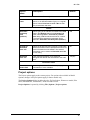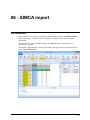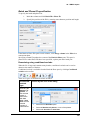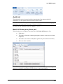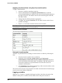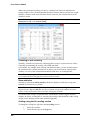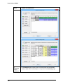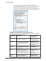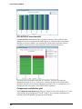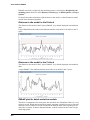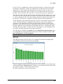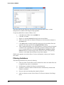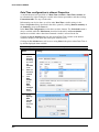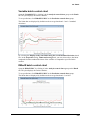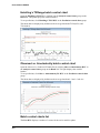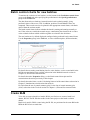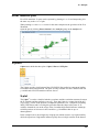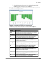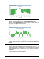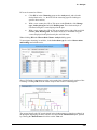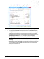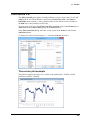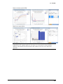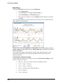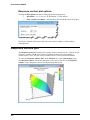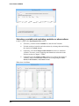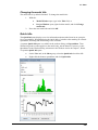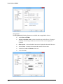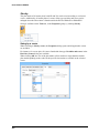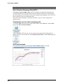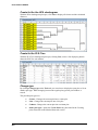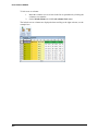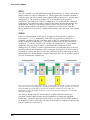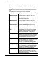
1
User Guide to SIMCA By MKS Umetrics Version 14 1992-2015 MKS Umetrics AB, all rights reserved Information in this document is subject to change without notice and does not represent a commitment on part of MKS Umetrics. The software, which includes information contained in any databases, described in this document is furnished under license agreement or nondisclosure agreement and may be used or copied only in accordance with the terms of the agreement. It is against the law to copy the software except as specifically allowed in the license or nondisclosure agreement. No part of this user guide may be reproduced or transmitted in any form or by any means, electronic or mechanical, including photocopying and recording, for any purpose, without the express written permission of MKS Umetrics. Umetrics patents and trademarks: SEQUENTIAL MODELING, US-7523384 MONITORING MULTIVARIATE PROCESSES, US-5949678 TOP-DOWN CLUSTERING/PLS-TREE®, US-8244498 DESIGN SPACE, US-8086327 MPMC, Pending RED-MUP®, VALUE FROM DATA®, OPLS®, O2PLS®, OPLS-DA®, O2PLS-DA®, PLS-TREE®, S-PLOT®, EZinfo®, FABSTAT®, SIMCA®, MODDE® ID #2055 User guide edition date: January 26, 2015 MKS Umetrics AB Stortorget 21 SE-211 34 Malmö Sweden Phone: +46 (0)40 664 2580 Email: [email protected] Welcome Welcome to the user guide for SIMCA 14. This is your guide to SIMCA and its capabilities. This user guide does not include in-depth background material to multivariate data analysis. For such information, see the book Multi- and Megavariate Data Analysis. Content The help is parted into 15 chapters, three appendices, and a reference list. 1. How to get started 2. Introduction to multivariate data analysis 3. Overview of SIMCA 4. Quick Access Toolbar 5. File 6. SIMCA import 7. Home 8. Data 9. Batch 10. Analyze 11. Predict 12. Plot/List 13. View 14. Plot and list contextual tabs 15. Scripting 16. Statistical appendix 17. Preprocessing appendix 18. Scripting appendix 19. References Table of Contents 01 - How to get started 1 Introduction.................................................................................................................... 1 License information ....................................................................................................... 1 What is in the package ................................................................................................... 1 System requirements ...................................................................................................... 1 Installation ..................................................................................................................... 2 Registration and activation .................................................................................................. 2 Starting SIMCA ............................................................................................................. 2 SIMCA projects ............................................................................................................. 2 Work process for regular projects .................................................................................. 3 Creating a new project by importing a dataset .................................................................... 4 Viewing and preprocessing the data .................................................................................... 4 Specifying the workset ........................................................................................................ 5 Specifying and fitting the model ......................................................................................... 6 Reviewing the fit and performing diagnostics ..................................................................... 6 Using the model for predictions .......................................................................................... 7 Work process for batch modeling .................................................................................. 8 Batch project overview........................................................................................................ 9 02 - Introduction to multivariate data analysis 11 Introduction.................................................................................................................. 11 Process data analysis .................................................................................................... 11 Process data properties ...................................................................................................... 12 Batch data analysis....................................................................................................... 13 Batch data properties ......................................................................................................... 13 Reorganization of 3D table before import ......................................................................... 14 Traditional data analysis: One or two variables at a time ............................................ 14 Multivariate approach .................................................................................................. 15 Summarizing a set of process variables ............................................................................. 15 Summarizing batch data .................................................................................................... 15 PCA - Principal Component Analysis ............................................................................... 16 PLS - Partial Least Squares Projections to Latent Structures ............................................ 16 OPLS and O2PLS - Orthogonal Partial Least Squares ...................................................... 17 Batch modeling in SIMCA ................................................................................................ 17 Conclusion ................................................................................................................... 23 03 - Overview of SIMCA 25 Introduction.................................................................................................................. 25 Application icon and symbol ....................................................................................... 25 Projects ........................................................................................................................ 25 Datasets ............................................................................................................................. 26 Workset ............................................................................................................................. 26 Models............................................................................................................................... 26 SIMCA window ........................................................................................................... 26 SIMCA ribbon description ........................................................................................... 27 v User Guide to SIMCA Ribbon ......................................................................................................................... 28 Quick Access Toolbar ....................................................................................................... 28 File .................................................................................................................................... 28 Home ................................................................................................................................. 29 Data ................................................................................................................................... 30 Batch ................................................................................................................................. 31 Analyze ............................................................................................................................. 32 Predict ............................................................................................................................... 32 Plot/List ............................................................................................................................. 33 View .................................................................................................................................. 34 Tools contextual tab .......................................................................................................... 35 Marked items contextual tab ............................................................................................. 36 Minimize/Expand the ribbon ............................................................................................. 38 View help .......................................................................................................................... 38 Workspace ................................................................................................................... 38 Clearing the Workspace .................................................................................................... 38 Shortcut menu .............................................................................................................. 38 Conventions ................................................................................................................. 38 Limitations in project names ............................................................................................. 38 Limitations in observation and variable identifiers ........................................................... 38 Case sensitivity ................................................................................................................. 39 Menu and tab reference syntax .......................................................................................... 39 Select and mark ................................................................................................................. 39 Vector and matrix representation ...................................................................................... 39 Missing values representation ........................................................................................... 39 Presentation of SIMCA results .................................................................................... 40 Plots for publications......................................................................................................... 40 Plots for reports ................................................................................................................. 40 04 - Quick Access Toolbar 41 Quick Access Toolbar .................................................................................................. 41 Customizing Quick Access Toolbar ............................................................................ 41 Removing buttons from Quick Access Toolbar ................................................................ 41 Adding buttons to Quick Access Toolbar.......................................................................... 42 Moving the Quick Access Toolbar .................................................................................... 42 Minimizing the ribbon ................................................................................................. 42 Copy and save plot ....................................................................................................... 42 05 - File 45 Introduction.................................................................................................................. 45 Info............................................................................................................................... 45 Project properties .............................................................................................................. 45 Encrypt .............................................................................................................................. 46 Compact project file .......................................................................................................... 47 Delete project .................................................................................................................... 48 Report................................................................................................................................ 48 New - Creating a new project ...................................................................................... 61 Open - Opening an existing project ............................................................................. 61 Opening pre-13 projects .................................................................................................... 61 Opening pre-13 filtered projects limitations ...................................................................... 61 Opening pre-13 batch projects .......................................................................................... 62 Recent projects and folders ............................................................................................... 62 vi Table Of Contents Save project ................................................................................................................. 62 Save project as ............................................................................................................. 63 Print ............................................................................................................................. 63 Help ............................................................................................................................. 64 Introduction ....................................................................................................................... 64 Activate SIMCA................................................................................................................ 64 HTML help ....................................................................................................................... 64 Umetrics on the Web ......................................................................................................... 65 About SIMCA ................................................................................................................... 65 Options......................................................................................................................... 65 SIMCA options ................................................................................................................. 65 Project options................................................................................................................... 71 Customize ribbon and keyboard shortcuts ......................................................................... 77 06 - SIMCA import 79 Introduction.................................................................................................................. 79 File ............................................................................................................................... 80 New spreadsheet................................................................................................................ 80 Save as in SIMCA import ................................................................................................. 96 Workspace ......................................................................................................................... 96 Print ................................................................................................................................... 97 Close ................................................................................................................................. 97 Options .............................................................................................................................. 97 Quick Access Toolbar .................................................................................................. 98 Home ........................................................................................................................... 99 Specifying identifiers ........................................................................................................ 99 Specifying data properties ............................................................................................... 104 Excluding/including rows or columns ............................................................................. 108 Apply formatting ............................................................................................................. 109 Column and row menus................................................................................................... 109 Finish and create project ................................................................................................. 110 Edit............................................................................................................................. 110 Rows and columns .......................................................................................................... 110 Merge .............................................................................................................................. 111 Sort .................................................................................................................................. 113 Find toolbar ..................................................................................................................... 113 View........................................................................................................................... 114 Audit trail ........................................................................................................................ 115 Batch & Phase pane phase part ....................................................................................... 115 Batch & Phase pane batch part ........................................................................................ 117 Class pane ....................................................................................................................... 118 Issues pane ...................................................................................................................... 118 Observations pane ........................................................................................................... 122 Summary pane................................................................................................................. 122 Variables pane ................................................................................................................. 123 Missing value map .......................................................................................................... 123 07 - Home 125 Introduction................................................................................................................ 125 Workset ...................................................................................................................... 125 Content ............................................................................................................................ 125 Workset statistics ............................................................................................................ 126 vii User Guide to SIMCA Correlation matrix ........................................................................................................... 127 New workset ................................................................................................................... 128 New workset as model .................................................................................................... 129 Editing the workset ......................................................................................................... 130 Deleting the workset ....................................................................................................... 131 Workset dialog ................................................................................................................ 131 Simple mode workset wizard .......................................................................................... 167 Change model type .......................................................................................................... 171 Model Options................................................................................................................. 176 Fit model .................................................................................................................... 184 Autofit ............................................................................................................................. 184 Two first components ...................................................................................................... 185 Add component ............................................................................................................... 186 Remove component ......................................................................................................... 186 Diagnostics & interpretation ...................................................................................... 187 Overview plots ................................................................................................................ 187 Summary of fit ................................................................................................................ 187 Scores .............................................................................................................................. 193 Loadings .......................................................................................................................... 201 Hotelling’s T2Range ....................................................................................................... 208 Distance to model ............................................................................................................ 209 Observed vs. predicted .................................................................................................... 211 Coefficients ..................................................................................................................... 211 VIP .................................................................................................................................. 214 08 - Data 217 Introduction................................................................................................................ 217 Import ........................................................................................................................ 218 Merge ......................................................................................................................... 218 Split dataset ................................................................................................................ 218 Transpose ................................................................................................................... 219 Delete dataset ............................................................................................................. 220 Generate variables...................................................................................................... 220 Generate Variables wizard .............................................................................................. 220 User generated functions ................................................................................................. 223 New variables from other dataset .................................................................................... 223 Generating variables in batch projects ............................................................................ 224 Local centering .......................................................................................................... 225 Importing local centering ................................................................................................ 225 Local centering of the predictionset ................................................................................ 227 Local centering missing .................................................................................................. 227 View imported local centering ........................................................................................ 227 Spectral filters ............................................................................................................ 227 Filtering limitations ......................................................................................................... 228 First, second, and third derivatives .................................................................................. 229 Multiplicative Signal Correction – MSC ......................................................................... 230 Standard Normal Variate – SNV ..................................................................................... 232 Row Center ..................................................................................................................... 233 Savitzky-Golay................................................................................................................ 234 EWMA ............................................................................................................................ 236 Wavelet Compression Spectral – WCS ........................................................................... 237 Wavelet Denoise Spectral – WDS................................................................................... 242 viii Table Of Contents Orthogonal Signal Correction – OSC .............................................................................. 245 Chaining filters ................................................................................................................ 249 Predictionsets and filtered datasets .................................................................................. 250 Time series filters ...................................................................................................... 250 Wavelet Compress Time Series – WCTS........................................................................ 250 Wavelet Denoising/Decimation – WDTS ....................................................................... 254 Dataset summary ....................................................................................................... 257 General page in dataset Properties .................................................................................. 258 Observations page ........................................................................................................... 258 Variables page ................................................................................................................. 259 Phases.............................................................................................................................. 261 Batches ............................................................................................................................ 261 Filter summary ................................................................................................................ 262 Trimming overview ................................................................................................... 262 Missing value map ..................................................................................................... 263 Spectra ....................................................................................................................... 263 Hierarchical models ................................................................................................... 264 Hierarchical models with OPLS or O2PLS ..................................................................... 265 Hierarchical models with blocks ..................................................................................... 265 Hierarchical base models reverts to non hierarchical ...................................................... 266 09 - Batch 267 Introduction................................................................................................................ 267 Batch control charts ................................................................................................... 267 Batch control chart background ...................................................................................... 268 Batch control chart plot and list customization ............................................................... 268 Excluding batches ........................................................................................................... 271 Score batch control chart ................................................................................................. 271 Variable batch control chart ............................................................................................ 273 DModX batch control chart............................................................................................. 273 Hotelling’s T2Range batch control chart......................................................................... 274 Observed vs. time/maturity batch control chart ............................................................... 274 Batch control charts list ................................................................................................... 274 Batch control charts for new batches ......................................................................... 277 Create BLM ............................................................................................................... 277 Selecting what to base the batch level dataset on ............................................................ 278 Selecting BEM variables for BL DS dialog .................................................................... 279 Raw Data Statistics Types dialog .................................................................................... 280 Batch condition datasets .................................................................................................. 281 Batch level datasets and missing values .......................................................................... 281 Sources of variation plot ............................................................................................ 282 BLM with batch conditions ............................................................................................. 282 BLM loading and contribution plots example ................................................................. 282 Time/maturity group plots ......................................................................................... 283 Observed vs. smoothed Y plot ........................................................................................ 283 Unaligned vs. aligned plot ............................................................................................... 284 Creating hierarchical models for batch level datasets ................................................ 285 Create Hierarchical Batch Models dialog ........................................................................ 285 Create hierarchical batch models results ......................................................................... 287 Hierarchical top level model ........................................................................................... 289 Batch Variable importance plot ................................................................................. 289 ix User Guide to SIMCA 10 - Analyze 291 Introduction................................................................................................................ 291 Biplot ......................................................................................................................... 292 Colors in the Biplot ......................................................................................................... 292 Inner relation plot ...................................................................................................... 293 S-plots ........................................................................................................................ 293 S-plot ............................................................................................................................... 293 S-line plot ........................................................................................................................ 294 SUS-plot.......................................................................................................................... 295 Contribution plots ...................................................................................................... 295 Scores/T2 contribution plot ............................................................................................. 296 Distance to model X contribution plot ............................................................................ 298 Distance to model Y contribution plot ............................................................................ 300 Y predicted contribution plot .......................................................................................... 301 Contribution plot for hierarchical top level models ......................................................... 302 Combined contribution plot for batch level model .......................................................... 303 Contribution plot from plot ............................................................................................. 304 Coefficient Y-related profiles plot ............................................................................. 305 RMSECV plot ............................................................................................................ 305 Residual normal probability plot ............................................................................... 306 Permutation plot......................................................................................................... 307 CV-ANOVA .............................................................................................................. 308 CV scores plot............................................................................................................ 308 HCA ........................................................................................................................... 309 Clustering of observations (matrix rows) ........................................................................ 310 Clustering of variables (matrix columns) ........................................................................ 312 HCA options ................................................................................................................... 314 Group dendrogram clusters marking tool ........................................................................ 314 Creating a PLS-DA or OPLS-DA model from plot marking........................................... 314 Creating class models from plot marking ........................................................................ 315 PLS-Tree .................................................................................................................... 315 Initializing a PLS-Tree .................................................................................................... 315 PLS-Tree wizard - removing outliers .............................................................................. 315 Clustering algorithm parameters ..................................................................................... 316 PLS-Tree resulting dendrogram ...................................................................................... 317 Group dendrogram clusters marking tool ........................................................................ 318 PLS-Tree model window and partial models .................................................................. 318 11 - Predict 319 Introduction................................................................................................................ 319 Specify predictionset.................................................................................................. 319 Specify Predictionset dialog ............................................................................................ 320 As dataset ........................................................................................................................ 321 As workset ...................................................................................................................... 322 Complement workset ...................................................................................................... 322 Class ................................................................................................................................ 322 Delete predictionset ......................................................................................................... 322 Batch predictionset .......................................................................................................... 322 Predictionset for filtered datasets .................................................................................... 323 Missing values in the predictionset ................................................................................. 323 x Table Of Contents Prediction list ............................................................................................................. 323 Properties in Prediction list ............................................................................................. 323 Y PS plots .................................................................................................................. 325 RMSEP ........................................................................................................................... 325 Y PS scatter plot .............................................................................................................. 326 Y PS line plot .................................................................................................................. 326 Y PS column plot ............................................................................................................ 327 Y PS list .......................................................................................................................... 327 Score PS plots ............................................................................................................ 327 Predicted score scatter plot .............................................................................................. 328 Predicted score line plot .................................................................................................. 328 Predicted score column plot ............................................................................................ 329 Predicted score 3D plot ................................................................................................... 329 Hotelling’s T2Range plot ........................................................................................... 330 DModX PS+ .............................................................................................................. 330 DModX PS+ - Distance to the model X-block ................................................................ 330 DModY PS - Distance to the model Y-Block ................................................................. 331 Control charts PS ....................................................................................................... 332 Contribution PS ......................................................................................................... 333 Scores/T2 ........................................................................................................................ 333 Distance to model X contribution plot ............................................................................ 334 Distance to model Y contribution plot ............................................................................ 334 Y predicted contribution plot .......................................................................................... 335 Contribution plot from plot ............................................................................................. 335 Time series PS ........................................................................................................... 337 Time series plot example ................................................................................................. 337 ROC - Receiver operating characteristic ................................................................... 338 Coomans' plot ............................................................................................................ 339 Classification list for class models ............................................................................. 340 Coloring in the Classification List ................................................................................... 340 Classification list for Discriminant Analysis models ................................................. 341 Coloring in the Classification List ................................................................................... 341 Misclassification table ............................................................................................... 341 Misclassification table for class models .......................................................................... 342 Misclassification table for Discriminant Analysis models .............................................. 343 Misclassification table Properties .................................................................................... 343 What-If....................................................................................................................... 344 Work process using What-If for regular models ............................................................. 345 Work process using What-If for batch evolution models ................................................ 345 Work process using What-If for batch level models ....................................................... 345 What-If pane ................................................................................................................... 346 What-If results................................................................................................................. 348 12 - Plot/List 351 Introduction................................................................................................................ 351 Name conventions ..................................................................................................... 351 Plot/List general dialog .............................................................................................. 352 Data series page............................................................................................................... 353 Transformation ................................................................................................................ 355 Control charts............................................................................................................. 362 What is a control chart? ................................................................................................... 362 xi User Guide to SIMCA Control Chart dialog ........................................................................................................ 363 Response contour ....................................................................................................... 372 Response contour plot options ........................................................................................ 374 Response surface plot ................................................................................................ 374 Wavelet structure ....................................................................................................... 375 Displaying Wavelet structure plot ................................................................................... 375 Wavelet power spectrum ........................................................................................... 376 Displaying Wavelet power spectrum plot ....................................................................... 376 Wavelet power spectrum example................................................................................... 376 Step response plot ...................................................................................................... 377 Creating a finite impulse response model........................................................................ 377 Displaying Step Response Plot........................................................................................ 379 Using an existing finite impulse response model ............................................................ 380 13 - View 383 Introduction................................................................................................................ 383 Show .......................................................................................................................... 383 Analysis advisor .............................................................................................................. 384 Audit trail ........................................................................................................................ 384 Favorites .......................................................................................................................... 386 Item information.............................................................................................................. 389 Marked items................................................................................................................... 390 Model window ................................................................................................................ 392 Notes ............................................................................................................................... 396 Observations pane ........................................................................................................... 396 Project window ............................................................................................................... 396 Quick info ....................................................................................................................... 399 Variables pane ................................................................................................................. 413 Full screen ....................................................................................................................... 413 Window group ........................................................................................................... 414 Skins .......................................................................................................................... 414 14 - Plot and list contextual tabs 415 Mini-toolbar - format plot .......................................................................................... 415 Mini-toolbar to customize plot text ................................................................................. 417 Managing the mini-toolbar .............................................................................................. 418 Tools tab .................................................................................................................... 418 Layout group ................................................................................................................... 419 Plot tools group ............................................................................................................... 439 Properties group .............................................................................................................. 447 Create group .................................................................................................................... 459 Add to favorites ............................................................................................................... 465 Add to report ................................................................................................................... 465 Marked items tab ....................................................................................................... 465 Create from marked items group ..................................................................................... 465 Drill down group ............................................................................................................. 467 Modify model .................................................................................................................. 472 Layout group ................................................................................................................... 475 15 - Scripting 479 Python scripting in SIMCA ....................................................................................... 479 Developer tab ............................................................................................................. 480 xii Table Of Contents Open the Developer tab ............................................................................................. 481 Python console ........................................................................................................... 481 Creating and accessing scripts ................................................................................... 481 Script favorites ................................................................................................................ 481 Add-Ins ........................................................................................................................... 482 SIMCA functionality available in Python .................................................................. 482 umetrics package content ................................................................................................ 482 Statistical appendix 485 Introduction................................................................................................................ 485 Fit methods background ............................................................................................. 485 PCA - Principal Components modeling .......................................................................... 486 PLS - Partial Least Squares Projection to Latent Structures modeling ............................ 487 OPLS/O2PLS - Orthogonal PLS modeling ..................................................................... 488 Cluster Analysis (CA), dendrograms, Hierarchical CA (HCA), PLS-Tree ............... 491 Hierarchical Cluster Analysis - HCA .............................................................................. 492 PLS-Trees ....................................................................................................................... 493 References cluster analysis .............................................................................................. 494 Vectors available in SIMCA ...................................................................................... 495 Variables and scores vectors ........................................................................................... 495 Observations and loadings vectors .................................................................................. 502 Function of component vectors ....................................................................................... 509 Function of lags vectors .................................................................................................. 512 Aligned vectors ............................................................................................................... 512 Batch vectors ................................................................................................................... 513 Formulas and descriptions ......................................................................................... 515 Prediction vectors ............................................................................................................ 515 R2Y, R2X, R2Yadj, R2Xadj ........................................................................................... 516 R2V and R2Vadj ............................................................................................................. 516 Q2 and Q2V .................................................................................................................... 516 Q2(cum) and Q2V(cum) ................................................................................................. 517 Leverages ........................................................................................................................ 517 RSD of observations and variables.................................................................................. 517 Relevance of variables .................................................................................................... 517 Hotelling's T2 .................................................................................................................. 518 Missing values correction factor ..................................................................................... 518 Missing values and PCA ................................................................................................. 519 Score and loading vectors ............................................................................................... 519 T scores (X): t1 vs. t2, ... ................................................................................................. 519 U scores (Y): u1 vs. u2, ... ............................................................................................... 519 T vs. U scores (X&Y): t1 vs. u1, ... ................................................................................. 519 P loadings (X): p1 vs. p2,... ............................................................................................. 519 W loadings (X): w1 vs. w2, ... ......................................................................................... 519 W* loadings (X): w*1 vs. w*2, ... ................................................................................... 520 C loadings (Y): c1 vs. c2, ... ............................................................................................ 520 WC or W*C loadings (X&Y): wc1 vs. wc2, ... ............................................................... 520 TPS scores (X): tPS1 vs. tPS2, ... .................................................................................... 520 Distance to the model ...................................................................................................... 521 Variable importance, VIP ................................................................................................ 525 Standard error and jack-knifing uncertainties.................................................................. 526 Coefficients ..................................................................................................................... 527 RMSEE, RMSEP and RMSECV .................................................................................... 529 xiii User Guide to SIMCA Transform page criteria .............................................................................................. 529 Automatic transformation criteria ................................................................................... 530 Scaling ....................................................................................................................... 530 Autoscaling ..................................................................................................................... 530 Block scaling ................................................................................................................... 530 Scaling weight calculation .............................................................................................. 531 Scaling of expanded terms .............................................................................................. 531 Scaling weights for transformed variables ...................................................................... 531 Scaling of variables with classes ..................................................................................... 531 Scaling of lagged variables.............................................................................................. 532 Scaling after changing the observation selection ............................................................. 532 Cross validation ......................................................................................................... 532 Cross validation for PCA ................................................................................................ 532 Cross validation for PLS, OPLS and O2PLS .................................................................. 532 Reference cross validation .............................................................................................. 533 Cross validation rules - Significant component ............................................................... 533 Cross validation rules - Non significant component ........................................................ 534 Cross validation rules for batches.................................................................................... 535 PLS time series analysis ............................................................................................ 535 References PLS time series ............................................................................................. 536 CV-ANOVA .............................................................................................................. 536 The ANOVA table .......................................................................................................... 537 References CV-ANOVA ................................................................................................. 538 ROC - Receiver Operating Characteristic .................................................................. 538 Fisher's exact test ....................................................................................................... 539 References Fisher's exact test .......................................................................................... 540 Control chart statistics ............................................................................................... 540 Nomenclature and notation in control charts ................................................................... 540 Target and standard deviation ......................................................................................... 541 S-plot background ...................................................................................................... 541 Reference S-plot .............................................................................................................. 542 Observation risk ......................................................................................................... 542 Preprocessing appendix 543 Preprocessing available in SIMCA ............................................................................ 543 Auto and cross correlation of variables or observations ............................................ 544 Reconstruction of wavelet compressed data .................................................................... 544 References auto and cross correlation ............................................................................. 545 Power spectrum density ............................................................................................. 545 Reference power spectrum .............................................................................................. 545 Wavelet transformations ............................................................................................ 545 Introduction ..................................................................................................................... 545 Overview of the wavelet transform ................................................................................. 546 Wavelet theory ................................................................................................................ 546 Multiresolution analysis, MRA ....................................................................................... 547 Wavelet families.............................................................................................................. 552 Wavelet compression or de-noising of signals ................................................................ 553 References for wavelets .................................................................................................. 556 Filtering and calibration ............................................................................................. 557 Derivatives ................................................................................................................. 557 Multiplicative Signal Correction (MSC).................................................................... 558 xiv Table Of Contents References for MSC ........................................................................................................ 558 Standard Normal Variate (SNV) ................................................................................ 558 Reference for SNV .......................................................................................................... 558 Orthogonal Signal Correction (OSC) ......................................................................... 558 Reference for OSC .......................................................................................................... 559 Scripting appendix 561 Introduction................................................................................................................ 561 Python tutorials .......................................................................................................... 561 Python software included ........................................................................................... 562 Using non-standard Python libraries with SIMCA .......................................................... 562 Graphic User Interface libraries ................................................................................. 562 Python script debugging ............................................................................................ 563 References 565 References for multivariate analysis .......................................................................... 565 Glossary 585 Index 591 xv 01 - How to get started Introduction This chapter holds information about the installation, including system requirements and such, as well as a short introduction to using SIMCA. Content License information What is in the package System requirements Installation Starting SIMCA SIMCA projects Work process for regular projects Work process for batch modeling License information Before installing the SIMCA product, carefully read the license agreement included with your SIMCA software package. In case you do not fully accept the terms of the license agreement, you should immediately return all parts of the package to your local supplier. What is in the package The SIMCA package contains the following: Installation files. SIMCA User Guide (.pdf). Installation instructions document. System requirements The minimum recommended system requirements: Pentium based computer (PC) with a 1.5 GHz or faster processor. 1 GB RAM or more. 1 User Guide to SIMCA 1 GB available hard disk space. 1024x768 screen resolution color display. Microsoft Windows 7 or 8. Graphics card that has hardware 3D acceleration and supports Open GL. Installation To install, follow the installation instructions delivered with the installation program. Note: You must have administrative privileges to be able to install the software. Registration and activation To register and activate, follow the instructions delivered with the installation program. See also the Activate subsection in the Help section in Chapter 5, File. Starting SIMCA Start SIMCA by double-clicking the icon or by starting it from the Start-menu or start screen. Continue by: Reading about the SIMCA software in the Help or User Guide. Both contain the same information. Starting a new project: click File | New. Running tutorial examples: Find the tutorials and tutorial datasets at the Umetrics website www.umetrics.com, or contact your Umetrics sales office. Select a suitable tutorial example, import the listed dataset used in the tutorial and follow the described steps. SIMCA projects What is a project? SIMCA is organized into projects. A project is a .usp file containing the results of the analysis of one or more datasets. Creating a new project Start a new project by importing one or more datasets. The default unfitted model is created when exiting the SIMCA import and is displayed in the Project Window. Project window The project window displays, for every model, one line summarizing the model results. The active model, the one you are working with, is marked in the project window. Default workset and model The default Workset consists of all variables and observations imported with the roles defined in the import. All variables are default centered and scaled to unit variance. How the variables were defined at import also defines which type the default model is. 2 01 - How to get started Creating a new model Unfitted models are implicitly created by SIMCA when: Specifying a workset or When changing the model type of a fitted model (fitted model is the active model). Activating and opening the model window To activate a model click it in the project window. All plots and lists created from the Home, Analyze and Predict tabs are created for the active model. To open the model window: Double-click it in the project window or Mark the model in the project window and then select the Model window check box on the View tab. The model window opens with the details of the model results, displaying one line per component. Opening the workset dialog To open the workset dialog of an existing model use one of the following methods: 1. Right-click the model in the Project Window and then select Edit Model x. 2. Click the Workset button in the Model Window. 3. On the Home tab click Edit | Model x. Work process for regular projects The work process in SIMCA consists of the following steps: Step Objective How to do it 1. Creating a new project. Click File | New | Regular project, and then select the dataset file or files to import. In the import spreadsheet define identifiers, X, Y, and qualitative variables etc. 2. Viewing and preprocessing the data. When warranted, preprocess your dataset using the available Spectral filters or Time series filters on the Data tab. 3. Specifying the workset and model type. On the Home tab, open the Workset dialog by clicking New/Edit in the Workset group. Select the variables and observations to include or exclude, define classes, transform, scale, or lag variables, and Trim-Winsorize the variables. Optionally select Model type before clicking OK to exit the dialog. 4. Fitting the model. In the Fit model group click Autofit. 5. Reviewing the results and performing diagnostics. Create plots found in the Diagnostics & interpretation group to detect trends, groupings, deviations, etc. 3 User Guide to SIMCA Step 6. Objective How to do it Using the model for predictions. On the Predict tab, use the predictionset to see how new data fit with the active model. Import another dataset with the new observations or use observations not included in the model as predictionset. Creating a new project by importing a dataset Create a new project by importing a dataset and specifying data properties in the SIMCA import spreadsheet. Selecting the dataset Click File | New | Regular project and then browse to find the file or files to import. To import from a database, Cancel the Open dialog and then click New spreadsheet | From database in the SIMCA import. You can import more than one dataset at the same time in SIMCA import by clicking File | New spreadsheet. Selecting another file adds a new spreadsheet to the SIMCA import. These spreadsheets are imported individually at Finish and you can create the workset from all or a selection of the datasets. Indicating file contents Specify Primary ID and as many Secondary IDs as desired for both variables and observations. Specify qualitative and date/time variables when present. Click Finish to import all currently open spreadsheets. Viewing and preprocessing the data Click Dataset, on the Home or Data tabs, to open any available dataset. Use the Data tab features to manipulate and preprocess datasets. Viewing the dataset Before preprocessing your data you may want to display the variables or observations in a plot. You can do this directly from the dataset spreadsheet by marking the variables or observations and on the Marked items tab clicking one of the plots in the Create from marked items group, or Drill down group or by opening the Quick Info pane on the View tab. To plot all the X observations as line plot, click Data | Spectra | dataset. Preprocessing the dataset Quick Info The Quick Info pane holds interactive plots tied to the dataset displaying variables or observations in the time or frequency domain. When displaying variables, Trimming / Winsorizing for a single or all variables is available. Generate new variables Generate new variables as functions of existing ones or from model results by clicking Data | Generate variables. 4 01 - How to get started Filter the dataset Filter your dataset (Data | Spectral filters), for example using: Multiplicative Signal Correction (MSC). Standard Normal Variate (SNV). Wavelet transform and compression. Wavelet transform time series data using compression, decimation/denoising. Specifying the workset The default Workset, at the project start, is the first dataset with variables defined as X and Y as specified at import, centered and scaled to unit variance. The associated model (unfitted) is listed in the project window. To fit the default model click Autofit in the Fit model group (Home tab). An unfitted model is generated by SIMCA when clicking OK in the Workset dialog and when switching model type for a fitted model by clicking the Change model type-button. New In the Workset group click New to create a workset of the entire firstly imported dataset with X and Y as defined at import and scaling as defined in File | Options | Project options. New as model In the Workset group click New as | Mx to use the workset of the selected model as starting point. Edit In the Workset group click Edit to open an already created workset. Modifying the workset To fit a model different from the default model, with maybe other or more datasets included, excluded variables and observations, or transformations, or different scaling, it is necessary to modify the default Workset. The following pages are available as tabs in the Workset dialog: Tab Functionality available Select data Selecting which datasets to include. Only available when there are more than one dataset to choose from. Overview Excluding variables and observations, redefining variables as X or Y, setting class belonging for observations, changing missing value tolerance and checking variables and observations for missing values. Variables Excluding and including variables. Defining variables as X or Y. Observations Including and excluding observations. Grouping observations into classes for classification. Transform Applying transformations for variables. Trim-Winsorizing variables. Note that trimming / Winsorizing the workset does not affect the dataset but just that particular workset. 5 User Guide to SIMCA Tab Functionality available Lag Defining lag structure. Expand Expanding terms with cross, square, and cubic terms. Scale Scaling variables. Spreadsheet Trim-Winsorizing variables. Note that trimming / Winsorizing the workset does not affect the dataset but just that particular workset. Simple mode You can select to have the workset wizard guide you through the specification and automatically fit the model by clicking the Use simple mode button in the Workset dialog. To turn it off, click the Use advanced mode button. Specifying and fitting the model Selecting the model type You can change the model type, when the workset specification allows it, by selecting another fit method than the default in the Model type box in the Workset dialog. Or by clicking Change model type in the Workset group and clicking a model type. Selecting a new model type after fit You can, after fitting the model, select a new model type. SIMCA then creates a new unfitted model with the selected model type. For example, if you have defined your Workset variables as X and Y, you can first fit a PCY (PC of the responses), then change the model type to PLS and fit a PLS model (another model) to the same data. Fitting the model Fit the model using one of the fitting types listed. Autofit Rule based fitting of the marked model or group of models. Two first Calculates two components whether they are significant or not. Often used to get a quick overview of the data. Add Calculate one component at a time. Here it is possible to force components to be calculated regardless of significance rules. Remove Remove the last component. Reviewing the fit and performing diagnostics After fitting, the whole spectrum of plots and lists are available for model interpretation and diagnostics. Important plots: 6 Summary plots 01 - How to get started Scores: t1 vs. t2, t1 vs. u1, etc. Loadings: p1 vs. p2, w*c1 vs. w*c2, etc. Hotelling's T2Range Coefficients Variable Importance (VIP) Important plots for diagnostics Distance to Model Residuals N-Plot (Analyze tab) Contribution plots Permutations (Analyze tab) Note: By default, all cumulative plots and lists are displayed for the last component. To select a different component for display in the plots, and/or a different variable, introduce the change in the Properties group, on the Tools tab. Using the model for predictions When you are content with your model you can use it for prediction. Importing datasets for prediction Later you may import additional data for use in predictions. Click Data | Import dataset. Building the predictionset Click the Specify-button on the Predict tab to build your predictionset from any or all datasets. You can display the predictionset as a spreadsheet or just plot or list results. If you do not specify a predictionset, the predictionset is by default the first dataset. Displaying the predictions Use any fitted model to: Classify the observations from the predictionset with respect to a PC or PLS model. Predict responses (values of Y variables) for the observations in the predictionset with respect to a PLS and OPLS model. All the prediction results (scores, y-values, etc.), computed with the active model, can be displayed as plots or lists. Plots and lists On the Plot/List tab you can find general plot and list commands. Here it is possible to plot and list any data, results and predictions. There are scatter, line, column, 3D scatter, list, time series, control charts, histogram, dot plot, normal probability plots, response contour, response surface, wavelets plots, and step response plots available. Note: With an active plot or list, use Change type group, on the Tools tab, to generate lists from plots and plots from lists. 7 User Guide to SIMCA Work process for batch modeling A SIMCA batch project consists of one or more batch evolution datasets and models and optionally one or more batch level datasets and models: 1. The batch evolution datasets have several observations per batch with the variables measured during the evolution of the batch. 2. The batch level datasets consisting of the completed batches, with one batch being one observation (matrix row). The variables of the batch level datasets are the scores, original variables (raw), or statistical summary variables (raw data statistics) of the batch evolution model, BEM, at every aligned time point folded out side-wise. The BLM may also contain batch condition variables. Batches may be divided into phases. The work process in SIMCA consists of the following steps: Step 1. Objective How to do it Creating a new project. Click File | New | Batch project. Select the dataset file or files to import. In the SIMCA import spreadsheet, define Batch ID, Phase ID, X, qualitative, time or maturity as Y, and if present Batch conditions. With phases, in the Batch & Phase pane optionally Rename, Merge, Delete, switch the order or time/maturity for the phases, or apply Conditional delete. Batch conditions can be imported with the batch evolution dataset, or as a separate dataset. SIMCA import assumes that a dataset with only one row per batch contains batch conditions. 8 2. Viewing and preprocessing the data. When warranted, preprocess your dataset using the available Spectral filters or Time series filters on the Data tab. 3. Specifying the workset. On the Home tab, open the Workset dialog by clicking New/Edit in the Workset group. Select the variables and observations to include or exclude, crop, transform, scale, expand or lag variables, and Trim-Winsorize the variables. Use the Variables page to configure the x and y-variables to the relevant phases, and y-variables smoothing/shifting/normalizing. 4. Fitting the model. Click OK in the Specify Autofit dialog automatically opened when exiting the Workset. Alternatively, mark the wrapper BEM and click Autofit. 5. Reviewing the batch evolution results and performing diagn ostics. Create BCC-plots found in the Analysis control charts group on the Batch tab to detect trends, groupings, deviations, etc. 6. Using the model for predictions. Create the BCC-plots found in the Prediction control charts group to see how new data fit with the active model. 01 - How to get started Step Objective How to do it 7. Creating the batch level dataset. On the Batch tab, click Create batch level and go through the wizard. 8. Importing batch conditions. To import batch conditions, click Data | Import dataset, select the file or files to import and specify batch ID. 9. Specifying the workset. The Workset dialog opens at Finish. Note that the Create a batch level model check box at the top of the Select data page is selected. Select the batch level and batch conditions datasets to use and then continue to the variables and observations pages to include or exclude etc. 10. Fitting the model. In the Fit model group click Autofit. 11. Reviewing the batch level results and performing diagn ostics. Create plots found on the Home tab to detect trends, groupings, deviations, etc. 12. Using the model for predictions. On the Predict tab, use the predictionset to see how new data fit with the active model. The batch evolution predictionset is automatically rearranged to a batch level predictionset. Batch project overview Batch evolution With batch data, you start by importing the batch evolution data and create the batch evolution model, BEM. Batch and phase identifiers and maturity variable In the data, you must have a Batch ID (identifier), indicating the start and end of the batch, and if phases are present, also a Phase ID. You may also have a variable indicating the evolution of the batch or phase and its end point. This variable can be Time or Maturity. You can have different Maturity variables for different phases. Default unfitted models Unfitted batch evolution models are implicitly created by SIMCA. When batches have phases, each phase is fitted as one PLS-class model with Time or Maturity as Y for each phase. By default all variables in a phase are centered and scaled to unit variance. Fitting the model Click Autofit with the BEM marked to fit all models at once. Reviewing the results Display the results of the analysis of the workset batches in the Analysis control charts group on the Batch tab, either as scores, DModX, Hotelling’s T2Range, predicted time or maturity, or as individual variables. 9 User Guide to SIMCA Predictions More datasets can be imported with new batches. The predictions can also be displayed in batch control charts in the same way by selecting the plot from the Prediction control charts group on the Batch tab. Batch level The batch level dataset is based on scores, original variables, or statistics of the original variables for completed batches, obtained from the BEM. The model created from these batch level datasets is named batch level model, BLM. Creating batch level dataset Create the batch level datasets by clicking Create batch level, in the Dataset group, on the Batch tab. Specify the properties of the batch level datasets to create. Creating batch level model Clicking Finish in the Create Batch Level Dataset wizard opens the Workset dialog with the Create a batch level model check box selected. Here you can select any batch conditions and batch level dataset created from the same BEM. To import batch conditions, click Data | Import dataset. You can change the default model type to any desired model type allowed by the workset specification. Alternatively specify hierarchical (Create hierarchical batch models on the Batch tab) or partial (select the Create partial models for each phase check box in the Workset dialog) models. Reviewing the results Display the results of the analysis of the workset batches in the Diagnostics & interpretation group, on the Home tab. Predictions The batch evolution predictionset is automatically rearranged to a batch level predictionset. This means that to make predictions for a BLM you select data from batch evolution datasets and SIMCA takes care of the rest. Project window for batch projects The project window displays, for every model, one line summarizing the model results. When batches have phases the PLS phase models (class models) are grouped in a wrapper, BEM. Both the BEM and BLM are grouped under an umbrella called BMxx, where xx is a sequential number. Use the tutorials to get a guided tour for building PC and PLS models. Find the tutorials in Downloads on www.umetrics.com. 10 02 - Introduction to multivariate data analysis Introduction This chapter gives an introduction to multivariate data analysis of regular and batch processes. Content Process data analysis Batch data analysis Traditional data analysis: One or two variables at a time Multivariate approach Conclusion Process data analysis Any investigation of a real process or system is based on measurements (data). Fifty years ago, measurement devices were expensive and few, and consequently the amount of data, measured on processes, was limited; a temperature and a pressure here, a flow rate there. The monitoring, display, and analysis of these few data was relatively simple, and a few running charts of the data provided all available information about the state of the process. Today, batteries of sensors and on-line instruments are providing data from all parts of the process in various forms, often at very short intervals. The masses of data are fed into computers, re-computed into moving averages (per minute, hourly, daily, weekly, etc.) and displayed and stored. This change from a situation with few, fairly infrequent measurements, to many, almost continuously measured variables has still not affected the manner in which process data are treated, potentially leading to large losses of information. With appropriate multivariate analytical methods, such as Principal Components (PC) and Projection to Latent Structures (PLS), and the recent extensions OPLS and O2PLS, in the SIMCA package, the masses of process data can provide easy to grasp graphical information about the state of the process, and relations between important sets of process variables. These multivariate methods make efficient use of all pertinent data, with little loss of information. 11 User Guide to SIMCA Process data properties Before going into the analysis of process data, it may be useful to discuss their nature. The data are usually measured at regular intervals over time; say every day, every hour, or every minute. These intervals are often different for different variables. We can recognize five categories, types, of process data: controlled process variables, result variables, characteristics of raw material, intermediate result variables, and uncontrolled variables. The variable types are described in the text that follows. Controlled process variables Related to the controlled setting of the conditions of the process, these are variables that, in principle, can be changed, thereby affecting the results, the output, of the process. We shall denote the values of these variables by xik (observation i, variable k). Examples of such variables are: T1, T2: the measured temperatures in reactors 1 and 2. P1, P2: the pressures in reactors 1 and 2. f12: the flow rate from reactor 1 to reactor 2. Result variables The availability of multivariate result variables (output, responses) measuring important properties of the products coming out of the process dramatically increases the possibilities to better understand and optimize a process. The result variables, are denoted yim (data point i, y-variable m). Examples of such variables are: yi1 = yield of main product (%). yi2 = impurity level (%). yi3 = amount of side product no. 1 (%). yi4 = tensile strength of product. Characteristics of raw material The characteristics of the raw material (inputs) are also denoted by x ik. These variables are often of great importance for the process and the product properties, but usually difficult or impossible to control. Examples of such variables are: Concentrations of iron, coal, nickel and vanadium in feed. Fiber length distribution in input pulp. Gas chromatographic and spectroscopic (NMR, IR, etc.) analysis of feed stock. Intermediate result variables Intermediate result variables are denoted by xik, yim, or zit. Examples of such variables are: 12 Viscosity of output from reactor 1 (=input to reactor 2). Concentration of oxygen in output from reactor 1. 02 - Introduction to multivariate data analysis Uncontrolled variables Uncontrolled variables are denoted by xik, or zit. Examples of such variables are: Air humidity, temperature of cooling water. Amount of oxygen in sparging nitrogen. The purposes of measuring the data on the process and its input and environment are to: Provide information allowing a better understanding of the process, relationships between different parts of the process, which chemical or other reactions occur inside reactors, etc. Yield information about the "state" of the process, recognizing trends, peculiarities, etc., all to keep the process under proper control. Discover how the output is affected by the process and input variables in order to improve product quality and minimize manufacturing costs, pollution, etc. Batch data analysis With batch processes, K variables are measured on N batches at regular time intervals. This gives a J x K matrix for each batch (J time points (X) times K variables). Consequently, a set of N normal batches gives a three-way matrix of dimension (N x J x K). Time One batch Batches Variables Figure 1: Three-way table of historical data of, for example, N batches with J time points, and K variables. Often the batches have different length (not shown in the picture) and may also be divided in phases. Batch data properties One of the differences between batch data and process data is that the batch process has a finite duration. Each batch can also go through several phases before completion. Since the batch data are collected batch wise they need reorganization before importing. 13 User Guide to SIMCA Reorganization of 3D table before import To be able to import the dataset, the 3-way data table has to be unfolded to preserve the direction of the K variables (see figure 2). The resulting matrix has nobs = N x J observations (rows) and K columns. Hence this matrix, X, has the individual observation as a unit, and not the whole batches. X Y Variables B1 B2 Batches B3 … Time Recorded variables: Ethanol, Temperature, Molasses flow, NH3 feed, Air flow, Tank level, pH. Bn Figure 2. The three-way matrix of figure 1 unfolded along the batch direction to give a two-way matrix with N x J rows and K columns. Each row has the data (xijk) from a single batch observation (batch i, time j, variable k). Traditional data analysis: One or two variables at a time To gain insight into the state of a process it is common to display important variables and their change over time (figure 3). This works fairly well with up to 5 to 10 variables, but thereafter becomes increasingly difficult to comprehend. Furthermore, these "time traces" reveal little about the relationships between different variables. Figure 3. Two of the variables plotted against time on horizontal axis. 14 02 - Introduction to multivariate data analysis Scatter plots of pairs of variables are common complements to time traces (figure 4). One hopes to identify correlations, thereby identifying important process variables causing changes in the output variables. The basic problem with pair-wise scatter plots is that they provide little information about the real relationships between, on the one hand, input and process variables, and, on the other hand, output variables. This is because the output (y) is influenced by combinations of the input and process variables (x). Figure 4. Scatter plot of y8* (impurity) against x2in (one of the inputs). Multivariate approach With multivariate methods, one can investigate the relations between all variables in a single context. These relationships can be displayed in plots as easy to understand as time traces and pair-wise scatter plots. The methods for multivariate process data analysis included in SIMCA are PC analysis and modeling, PLS modeling, OPLS modeling, O2PLS modeling and more. The principles and mathematics of the fit methods are briefly described later in the introduction, and more thoroughly in the Statistical appendix. References are also given to additional pertinent literature. Here we will indicate how to use these methods to solve typical problems in process data analysis. Summarizing a set of process variables Data measured on a process are usually stored in some kind of database. A process database containing the values of K variables for N data points can be regarded as a table, a matrix. We denote the whole table by X. Each column in the table corresponds to one variable (xk), and one row (xi) corresponds to the values observed at one point in time. Inputs or outputs or both can be displayed in multivariate control charts. Summarizing batch data Data measured batch wise are also often stored in some kind of database. One of the differences between batch data and process data is that the batch process has a finite duration. Each batch can also go through several phases before completion. Inputs or outputs can be displayed in batch control charts. 15 User Guide to SIMCA PCA - Principal Component Analysis Principal component analysis of a data table gives vectors of scores, with values tia, which summarize all the variables entering the analysis. It is customary to calculate two or three score vectors, and then plot them against each other (tt-plots). This gives a picture that is the best summary of the process behavior over time! In this plot we can see trends, unusual behavior and other things of interest. With experience, one will be able to recognize an area in this PC score plot in which the process remains under "normal" operation, thus providing a multivariate control chart. The score plot in combination with the loading plot, indicate the responsible variables for deviations from normal operation. The PCA also gives residuals, deviations between the data and the PC model, named DModX. When these residuals are large, this indicates an abnormal behavior in the process. To see this, we make a plot of the residual standard deviation, DModX (residual distance, root mean square). Observations with a DModX larger than the DCrit are outliers. When DModX is twice DCrit they are strong outliers. This indicates that these observations are different from the normal observations with respect to the correlation structure of the variables. PLS - Partial Least Squares Projections to Latent Structures Relating the result variables to input and process variables A common problem is “process diagnostics”. That means identifying those input and process variables, X, that are “responsible” for the change in output variables, result variables, Y. For this purpose, one often attempts to use multiple regression, which, however, leads to great difficulties because process data usually do not possess the correct “properties” for regression modeling. In particular, regression deals with each result variable (ym) separately, and one therefore ends up with a set of models, one for each output of interest. This makes interpretation and optimization difficult or impossible. To allow strict interpretation of "cause and effect", the data should be collected in a careful experimentation using statistical design (with software such as MODDE). To search for relationships between input and output in process logs is risky and often less successful. This is because a process does not provide data with good information content when the important factors are well controlled within small "control intervals". PLS - Scores PLS modeling has been developed explicitly for this type of situation with numerous, often-correlated input and process variables and several to many result variables. One just specifies which variables in the database that are predictors (X), and which variables are dependent (Y), and PLS finds the relation between the two groups of variables. The PLS model is expressed as a set of X-score vectors, Y-score vectors, X-weight and Y-weight vectors, for a set of PLS model dimensions. Each dimension (index a) expresses a linear relation between an X-score vector (ta) and Y-score vector (ua). The weight vectors of each model dimension express how the X-variables are combined to form ta, and the Y-variables are combined to form ua. In this way the data are modeled as a set of "factors" in X and Y and their relationships. Plots of the scores and weights facilitate the model interpretation. 16 02 - Introduction to multivariate data analysis PLS - Loadings The PLS analysis results in model coefficients for the variables, called PLS-weights or loadings. The loadings for the X-variables, denoted w, indicate the importance of these variables, how much they “in a relative sense” participate in the modeling of Y. The loadings for the Y-variables, denoted by c, indicate which Y-variables are modeled in the respective PLS model dimensions. When these coefficients are plotted in a w*c plot, we obtain a picture showing the relationships between X and Y, those X-variables that are important, which Y-variables are related to which X, etc. PLS - Residuals Analogous to PC, PLS gives residuals, both on the Y-side and on the X-side. The standard deviations of these (residual distances) can be plotted just as for PCA to give a third "SPC" plot (Statistical Process Control) showing if the process is behaving normally or not in DModX and DModY plots. OPLS and O2PLS - Orthogonal Partial Least Squares OPLS is an extension of PLS and addresses the regression problem. OPLS separates the systematic variation in X into two parts, one part that is correlated (predictive) to Y and one part that is uncorrelated (orthogonal) to Y. This gives improved model interpretability. In the single-Y case, there is only one predictive component, and all components beyond the first one reflect orthogonal variation. However, with multiple Yvariables there can be more than one predictive OPLS component. O2PLS is yet another extension of PLS and addresses the data integration problem. Thus, in the two-block (X/Y) context, O2PLS examines which information overlaps between the two data tables and which information is unique to a specific data table (X or Y). O2PLS accomplishes this task by a flexible model structure incorporating three types of components, that is, (i) components expressing the joint X/Y information overlap, (ii) components expressing what is unique to X, and (iii) components expressing what is unique to Y. For both OPLS and O2PLS the different components are interpretable the usual way, since the scores, loadings, and residual-based parameters with a familiar meaning are preserved. Batch modeling in SIMCA A SIMCA batch project consists of one or more batch evolution models, BEM, and optionally one or more batch level models, BLM: 1. The BEM has several observations per batch with the variables measured during the evolution of the batch. Batch evolution models are commonly applied for real time process monitoring. 2. The BLM consists of the completed batches, with one batch being one observation (matrix row). The variables of the BLM are the scores, original variables, or summary variables (statistics of the original variables) of the BEM at every time point folded out side-wise. Batch level models are commonly applied to investigate variations between batches, sites, campaigns or to study impact of process variations on product quality. 17 User Guide to SIMCA A BM, sequentially numbered, holds the BEM and the BLM-models built on datasets created from that BEM. Batches may be divided into phases. Batch evolution modeling When importing the dataset in SIMCA, an index y-variable starting at 0 is constructed if no maturity is specified. This is the "relative local batch time". The default model, after completed import in SIMCA, is a PLS model for the centered and scaled X and y, or "relative local batch time" as y if no other y was specified. If a maturity variable, recorded relative to the start of each batch, was defined as y, it is the variable used as y. When fitting the batch evolution PLS model, “Autofit” will stop when 85% of X has been explained, but will also give at least 3 components, as long as the number of components does not exceed number of variables/2. This is necessary in order to ensure that much of the X-matrix is "explained". This results in an (nobs x A) score matrix, T, plus PLS weight and loading matrices W and P (of dimensions K x A). Modeling the evolution of batches in the workset At the start of a batch project, when phases are present, the BEM workset is created with an unfitted model for every phase. The BEM is the wrapper grouping all the PLS class models (one for every phase). Maturity or time, as specified for each phase, is used as Y, the other variables as X, and all are centered and scaled to Unit Variance. When batches have no phases, there is only one model in the BEM, with time or maturity as Y and all other variables as X, centered and scaled to Unit Variance. Note: A model is positioned in a BEM only when the data was imported as batch and it is a PLS model with one variable specified as y (Time or Maturity). 18 02 - Introduction to multivariate data analysis To fit the model(s), mark the BEM and click Autofit. The BEM is built on the good batches when the goal is to define a process monitoring model with the ideal evolutionary trace. Around this trace, 3 SD limits are used to define the acceptable variation. Examine the batch evolution models using the Batch control charts (BCC), starting with the Variable BCC to ensure that the process data is good and reliable for all batches. Look for outlier batches in batch control chart scores and/or the DModX plots. Interpret deviating batches with contribution plots. Batches with different length Alignment of data is done differently depending on configuration of the time/maturity variables. For batches of similar length the impact is small. The default y configuration aligns the batch length by cutting the longer batches at median (or average) batch length. Batches that are shorter than the median (or average) batch, are filled up with the last value up to the median batch length. The used length in average batch is the shorter of the median batch length and the average batch length rounded down. Batches with several phases When batches have several phases, observations are organized in classes, one class for every phase. Separate PLS or OPLS-class models are fitted for every phase. Smoothing the maturity variable If a maturity variable is used as the response variable Y, indicating the degree of completion of a phase, the maturity variable has to be strictly monotonic in a given phase, but can be ascending or descending. Different phases can have different maturity variables. Different phases can have ascending or descending maturity. When maturity variables are not strictly monotonic, they are smoothed within each phase. The smoothing is done by fitting a constrained quadratic polynomial, using a piece wise least squares algorithm. This is to ensure that the maturity is strictly monotonic within a phase. The smoothed maturity is used by default, both as the response variable Y, and for alignment. 19 User Guide to SIMCA A difference between SIMCA 14 and SIMCA 13 is that in SIMCA 14 and later the smoothing increment was decreased so that when a maturity isn't increasing/decreasing it appears flat visually (in plots). That was sometimes not the case in SIMCA 13 and earlier. Result variables The score matrix T is a good summary of X, and PLS focuses this summary on y (local time). Hence the first column of t (t1) will contain strong contributions of those Xvariables that vary monotonously with y, i.e., either increase or decrease with time. The second component (t2) is an aggregate mainly of those variables that change “quadratically” with time, i.e., first go up to a maximum, and then decrease, or first go down, and then up. The third component catches the variables having a cubic behavior, etc. The value of "local time" predicted by the PLS model (with the number of components determined by cross validation ), ypred, is very suitable as a "maturity index" that can be used to indicate how far the batch has evolved, if it is ready for termination, etc. For the OPLS model all variation relating to Y is captured in the first component. Calculating limits to build control charts To monitor the evolution of new batches, one calculates the typical evolution trace of a normal batch in terms of the scores, DModX, etc. This is in short done as follows: 1. Reorganization: First the scores of the BEM are chopped up and reorganized so that the scores of one batch form one row vector (t1 followed by t2 for PLS and to1 for OPLS, followed by t3 for PLS and to2 for OPLS, etc.) in a matrix ST. This matrix has N rows (one per batch) and A x J (AJ) columns from the A score vectors and the J "time points" per batch. When batches have phases, the scores of each batch are collected from the different PLS phase models and the calculations are done separately for the different phases. t1 Average Avg + 3 sd StDev Avg – 3 sd Batch Time Figure 4. The score values for each batch are arranged as row vectors under each other, giving an N x (J x A) matrix, S T. Above we see only the first part of ST corresponding to the 1st component (t1). From this matrix one calculates the averages and standard deviations (SDs) of the matrix columns, and then control intervals as the averages 3 SD. 2. 20 Calculating tolerance limits for score batch control charts: Now the matrix ST is used to derive minimum and maximum tolerated values at each time point (j) of tj1, tj2, tj3…, tjA from the column averages and standard deviations of ST, as indicated in figure 4. In MSPC one would typically use tolerance intervals of the average 3 SD at each time point. Hence, we now have for each score vector an average trace with upper and lower tolerance limits (figure 4). This specifies the normal evolution traces, one for each score component, of new batches. 02 - Introduction to multivariate data analysis 3. Calculating tolerance limits for y predicted batch control chart: An additional trace is constructed from the values of predicted y (local time or maturity), for each time point of each batch. The predicted y-values should be fairly close to the "real" y-value for a batch evolving at the "normal" rate. SIMCA forms a matrix RY with the traces of predicted y of each batch as rows, and then analyzing it in the same way as ST above, and gives tolerance intervals of ypred for each time point. 4. Calculating tolerance limits for DModX batch control chart: An additional trace is constructed from the values of the residual standard deviation (distance to the model, DModX), for each time point of each batch. The residual standard deviation (DModX) is calculated from the residuals, i.e., after subtracting ti x P' from the scaled and centered observation x-vector. For an observation to be judged OK (non-deviating), DModX should be smaller than a critical limit, Dcrit calculated from the F-distribution. Note: When batches have phases, the limit calculations are done by phase. Monitoring the evolution of new batches The batch evolution data of new batches are inserted into the PLS or OPLS model, giving predicted values of the score values t1 to tA. These results can now be plotted in the appropriate batch control charts, with limits derived as described in the Calculating limits to build control charts subsection. These charts indicate whether the batches are starting normally or not. If the values are outside the normal ranges, contribution plots based on the x-values or the residuals indicate which variables together are related to the deviations. In addition, the PLS model gives predicted values of y (local time or maturity index). Plotting ypred vs. yobs gives a very interesting indication of whether the batches are developing too quickly (over-mature, ypred > yobs) or too slowly (under-mature, ypred < yobs). When batches have phases, the appropriate PLS phase model is used to predict the t scores of every phase. The scores are collected for every batch and results are plotted in the control charts. Batch level modeling This section describes modeling of entire batches as observations (rows) using batch level modeling. Why batch level modeling? Batch level modeling may be advantageous in the case that the measurement of Y is laborious and time consuming, and one wishes to make an initial fast quality assessment before the real Y is available. This is often the case in biotechnological production, where extensive analysis and testing of the final products is made before acceptance (or rejection). The batch level model (BLM) also allows the full interpretation of the batch data. Groups of batches may be discovered, outliers will be found, etc. Critical time periods will be indicated by "periods" of large weights, loadings, and VIP values. Analogously, important factors in the batch conditions will stand out. Creating the batch level model The batch level model can be created based on scores, original variables, summary variables (raw data statistics), duration and endpoint, plus batch conditions (Z). 21 User Guide to SIMCA Modeling batch level The objective of batch level modeling is to make a model of the whole batch in order to understand how Y is influenced by the combination of batch conditions and the batch evolution. This model will be based on (when available) the batch conditions (Z), the evolution trace matrix ST, and when applicable the properties and quality of the completed batch (Y), as shown in figure 5. The resulting model is used to predict Y for new batches from their batch conditions and their evolution traces. X Back ground Data Scores t1, t2, t3 or original variables Data Y Final Results Data Figure 5: The data for batch level modeling. Each row has the data from one batch. The left matrix contains data describing initial batch conditions. The middle matrix contains the unfolded scores/raw variables, which describe the evolution of each batch. The optional right matrix (Y) contains the responses, the properties of the complete batch such as yield, purity, activity, etc. In the case that Y-values do not exist, the X-matrix can still be used to develop a PC model. We see that this is the same type of model as the X-part of PLS in the batch evolution model. The difference is that in PCA the scores (T) are calculated to give an optimal summary of X, while in PLS this optimality is somewhat relaxed to make T scores better predictors of Y. This PC model can then be used to classify new batches as normal (similar = well fitting to the PC model) or non-normal (far from the model). Predicting results or classifying whole new batches The batch level model is used to predict quality of the final batch (Y), or classify the batch as normal good batch or bad batch or predict their final quality. If you have fitted hierarchical models of the batch level data at different percentage of completion, you can classify or predict the final quality of new batches as they are evolving when they reach the percent of completion of the models. If the values are outside the limits, contribution plots indicate which variables together are related to the deviations. Create a batch level model When creating a batch level dataset, clicking Finish opens the Workset dialog with the Create a batch level model check box selected. Select the datasets to use and then use the other pages in the dialog for editing the workset as desired. Clicking OK in the Workset dialog creates the unfitted BLM. Note: Changing the order of the selected datasets resets the workset. Additionally selecting/clearing dataset check boxes in the Select data page may result in resetting the workset. When resetting the workset, all variable and observation/batch settings are cleared along with any changes in transformations, lags, expansions, scaling and trimming and the result is the default workset. 22 02 - Introduction to multivariate data analysis Hierarchical batch models For batch level datasets you can fit hierarchical models of the whole batch, for different levels of completion: One model for each phase and component in BEM. One model for each phase. Sequential models covering parts of the batch completion, for example for 25%, 50%, 75% and 100% completion for models without phases. These models can predict the final batch quality or classify the batch, before the batch is finished. Conclusion Projection methods such as PCA, PLS, OPLS and O2PLS find the information in masses of process data by projecting these data down on a few "scores". These scores provide a very good summary of process data tables (X and Y), and score plots display this in an easy to grasp form. The coefficients of the projections, i.e., how the variables are combined to form the scores, are called loadings or weights. Their plots show the importance of the variables, their similarity, their connection, and other things of interest. The parts of the data not seen in the score plots, i.e., the residuals, are displayed (in summarized form) in the DModX and DModY plots (row residual standard deviations). For further reading, see the Multi- and Megavariate Data Analysis book and the reference list. 23 03 - Overview of SIMCA Introduction This chapter describes the following: Application icon and symbol. SIMCA projects. SIMCA window interface. Ribbon content. Shortcut menu. Conventions including limitations and missing values representation. Presentation of SIMCA results Application icon and symbol The application icon is a purple circle with a white S inside (below). Projects Multivariate data analysis in SIMCA is organized into projects. You can think of a project as a file folder containing all the information related to the analysis of a number of datasets. Projects are by default named after the first selected dataset in SIMCA import. This information is organized in the following components: Datasets used for the analysis. Other datasets used for predictions and model validation. Workset and multivariate models. 25 User Guide to SIMCA Datasets For continuous processes, the data are observations made sequentially in time, usually at a constant sampling interval. Such data are called time series. In the analysis of time series, the observed outcome at time t is often modeled as a function of the previous observations at time t1, t2, etc. With PLS, the time series analysis is performed by creating lagged variables, i.e., variables shifted in time, and fitting the model. For PLS time series analysis to give correct results the observations must be contiguous in time (the sampling interval is constant), and with no missing observations. A batch process has a finite duration. Each batch can go through several phases before completion. Since the batch data are collected batch wise they need reorganization before importing. Workset A workset is a subset or all of the data in the selected datasets with a particular treatment of the variables, i.e., role (predictor variables X, or responses Y), scaling, transformation, lagging, etc. The workset is by default the first dataset with all imported variables and observations included and the variables centered and scaled to unit variance, for regular projects. For batch projects the default workset is all batch evolution datasets imported when creating the project. When you define a workset, SIMCA creates an unfitted model, and both the model and the workset are identified by the same name. Models Models are mathematical representations of your process and are developed using the data specified in the workset and with a specified model type, for example, PCA-X, PCA-Y, PCA-X&Y, PLS, etc. With a specified workset, you may be able to fit several models by selecting different model types. For example, if you have specified a workset by defining the X-variables (predictors) and the Y-variables (responses), you may first fit a PC of the responses (Yblock) and then fit a PLS model, by just selecting another model type. Models are created by SIMCA when: 1. You specify a workset, New/New as model. 2. You make a selection under Change model type with a fitted model. You work with one model at a time, the active model. This model is marked in the Project Window and its name and title are displayed in the caption of the project window. There is always an active model. You may have several models open, but only one of them is active. SIMCA window The SIMCA window consists of the ribbon with regular and context tabs, the quick access toolbar, and panes. 26 03 - Overview of SIMCA SIMCA ribbon description Description of the ribbon using terminology according to Microsoft: The File tab holds commands that involve doing something to or with a document, such as file-related commands. Quick Access Toolbar is a customizable toolbar that displays frequently used commands. Core tabs are the tabs that are always displayed. Contextual tabs are displayed only when a plot or list is open, Tools, or when items are marked in a plot or list, Marked items. Galleries are lists of commands or options presented graphically. A resultsbased gallery illustrates the effect of the commands or options instead of the commands themselves. Dialog box launchers are buttons at the bottom of some groups that open dialog boxes containing features related to the group. 27 User Guide to SIMCA Ribbon Available functionality can be accessed through the SIMCA interface. The SIMCA interface includes: the Quick Access Toolbar the regular tabs File, Home, Data, Batch, Analyze, Predict, Plot/List, and View the context tabs Tools and Marked items and the help-button On the tabs the commands are parted in groups. Some of the groups have a dialog box launcher which opens a dialog closely connected to the features in the group. For a short introduction see the sections that follow here. For more, see the respective chapters. Quick Access Toolbar The Quick Access Toolbar allows you to have your favorite commands easily accessible. File The following is available on the File tab: 28 Info - Manage allows encrypting and compacting the project. Report creates a report. New | Regular project/Batch project – Creates new SIMCA projects after selecting a dataset in SIMCA import. If you have skins installed, application specific project types can be selected here automatically switching to the application skin. Open – Opens old project. Contains Recent projects and Recent folders lists. Save – Saves the current project. Save as – Saves the current project to the specified path and name. Print - Automatically displays a preview of the active window. Print setup and other print feature are available. Close – Closes the current project. Help - Contains license info, the possibility to Activate, and support features such as the help file. Options - Contains SIMCA options with the current default options for SIMCA, Project options with the current default options for the current project, and Customize which enables customization of the ribbon. 03 - Overview of SIMCA Home On the Home tab you can change the model type, fit the model and review the fit. Plots and lists to analyze the model are available from this tab. On the Home tab the following is available: Dataset group Dataset – Lists and opens all available datasets. Workset group The workset is a working copy of the selected datasets with certain properties defined. Note: The datasets are NOT affected when you exclude variables/observations or by any other operation in the workset. In the Workset group the following is available: Statistics | Workset statistics – Displays statistics of selected variables of the active model. Statistics | Correlation matrix – Displays the correlations between the variables for the active model. New – Creates the default workset consisting of the first listed dataset with the variables set as X or Y as specified at import, and scaled according to the specified scaling in Project Options. For batch all batch evolution datasets imported when creating the project are included in the default workset. New as – Creates a new workset as a copy of the selected model. Edit – Opens the selected specified model for editing. If the model has already been fitted that model will be replaced by a new unfitted model at OK. Delete – Deletes the selected workset, and consequently also the model. Change model type - Displays the available model types: Overview - PCA-X, PCA-Y, PCA-X&Y, O2PLS Regression - PLS, OPLS Discriminant analysis - PLS-DA, OPLS-DA, O2PLS-DA Class - PCA, PLS, OPLS, O2PLS Clustering - PLS-Tree Model options – Available from the dialog box launcher (arrow beneath the Change model type arrow) and displays the options of the active model. Fit model group For the model or model group (CM/BEM): Autofit – Autofits according to the autofitting rules. Two first – Calculates the two first components. Add – Calculates the next component. Remove – Removes the last component. 29 User Guide to SIMCA Diagnostics & interpretation group Overview: Displays the 4 default plots X/Y Overview, Scores, Loadings, DModX. Summary of fit: Summary of fit plot and list – Displays the cumulative fit over all variables for each component. X/Y overview plot and list – Displays the cumulative fit of all variables for each x-variable for PCA and each y-variable for PLS, OPLS and O2PLS. X/Y component – Displays the fit of a variable for each component. OPLS/O2PLS overview - Displays OPLS and O2PLS specific R2. Component contribution – Displays the contribution of a model component to the fit. Review the fit and investigate diagnostics: Scores t1 vs. t2, Num vs. t1, etc. – Displays trends, groupings, outliers. Loadings p1 vs. p2, w*c1vs. w*c2, etc. – Displays important variables, variable correlations. Hotelling’s T2 – Displays a measure of how far each observation is from the model center. DModX for X or Y – Displays the distance from the observation to the model, by default after the last component. Observed vs. predicted – Displays the actual value versus that observation predicted by the model for the selected response (y) variable. Coefficients – Displays the coefficient of the model for each response (y) variable cumulatively over all components. VIP – Displays the overall importance of each variable (x) on all responses (Y) cumulatively over all components. Data On the Data tab the following is available: Import dataset – Imports selected datasets. Dataset – Lists and opens all available datasets. Modify dataset group 30 Merge – Merges the selected datasets and deletes the second dataset (source). Split - Splits the selected dataset as specified in the dialog. Only available for independent datasets. Transpose – Transposes the selected dataset and deletes dependent models and datasets. Not available for batch projects or dependent datasets. Delete dataset - Deletes the selected dataset and any dependent models and datasets. 03 - Overview of SIMCA Generate variables – Creates new variables as functions of the existing ones or from model results. Local centering - Import local centering or View already imported local centering data. Filters group Spectral filters - Filters the selected dataset using the selected filter creating a dataset in the current project. The available filters are: Derivative (1st, 2nd, and 3rd derivative), Multiplicative Signal Correction (MSC), Standard Normal Variate (SNV), Row Center, Savitzky-Golay, EWMA, Wavelet Compression, Wavelet Denoising, Orthogonal Signal Correction (OSC) and chained filters. Time series filters - Time series filters the selected dataset using Wavelet Compress Time Series and Wavelet Denoising/Decimation creating a new dataset in the current project. Summary group Dataset summary – Displays a summary of the performed filtering. Available for filtered datasets. Missing value map - Displays an overview of a dataset with respect to missing values. Trimming overview – Opens an overview window of the trimming. Only available after trimming. Spectra - Displays ObsDS, for the variables specified as X, of the selected dataset. Base model group Hierarchical - Specifies the current model as hierarchical base model creating a hierarchical dataset. Non hierarchical - Removes the hierarchical base dataset. Batch On the Batch tab batch related commands are available. Analysis control charts and Prediction control charts groups Batch control charts that display scores, distance to model, variable, Hotelling’s T2, or predicted y with limits in plots and lists for models and predictions (BEM only). Time/Maturity group Observed vs. smoothed Y - Displays the maturity for selected batch in original and treated form (BEM only). Unaligned vs. aligned - Displays the selected vector for the selected batch aligned and unaligned (BEM only). Dataset group Create batch level – Creates the batch level dataset according to the selections made by the user. Available with a BEM marked only. 31 User Guide to SIMCA Create hierarchical batch models – Creates hierarchical batch models according the selections in the dialog. Only available for batch level datasets. Variable summary group Variable importance plot – Displays the overall importance of the variable over the whole evolution on the final quality of the batch. Available for BLM only. Analyze On the Analyze tab the analysis related features not available on the Home tab are available. Analysis group Biplot – Displays scores and loadings superimposed. Inner relation - Displays t1 vs u1, t2 vs u2 etc. S-plots - S-plot, S-line, and SUS-plot display p in forms informative for OPLS with one Y. Contribution – Displays variables likely to be causes for upsets in the score, DModX, Hotelling’s T2Range, or predicted response plots. RMSECV - Indicates predictive power. Y-related profiles - Coefficients rotated displaying the pure profiles of the underlying constituents in X using the assumption of additive Y-variables for OPLS and O2PLS. Residuals N-plot – Displays the residuals on the normal probability chart for the selected Y. Validate group Permutations – Displays the validity and the degree of overfit for the model (only PLS). CV-ANOVA – For assessing the reliability of the model. CV scores - Displays the cross-validated complement to the regular scores plot Clustering group HCA – Displays the clusters from the cluster analysis in a tree diagram. PLS-Tree - Displays the cluster analysis result using PLS-Trees. Predict On the Predict tab you can select a predictionset, display the predictionset as a spreadsheet, and display the prediction results using the active model. The following is available: Specify predictionset group 32 Specify – Defines the predictionset in the Specify Predictionset dialog. 03 - Overview of SIMCA As dataset - Predictionset is the selected dataset. As workset - Predictionset is the current workset. Complement workset/Complement WS batches - Predictionset is the observations/batches not included in the current model. Class - Predictionset is the selected class. Delete predictionset - Deletes the selected predictionset. List group Prediction list – Displays the predictionset, some predicted vectors such as membership probability, scores, and the predicted response for PLS models. Plots group Y PS – Displays the predictions for the selected response (y). Scores PS – Displays the predicted scores. Hotelling’s T2 PS – Displays a measure of how far the predicted value for the observation is from the center DModX PS+ for X or Y – Displays the distance from the predicted value for the observation to the model. Control charts PS – Displays the selected vector in the selected control chart: Shewhart, CUSUM, EWMA, or EWMA/Shewhart. Contribution PS – Show variables likely to be causes for upsets in the predicted score, distance to model X, Hotelling’s T2Range, or predicted response plots. Time Series PS - Displays the selected vector in a line plot. ROC - Displays FPR (False Positive Rate) and TPR (True Positive Rate) for the marked DA or class models. Coomans' plot – Shows class separation for two selected models. Classification list - Displays the classification of a predictionset with respect to all the class models. Misclassification table – Summarizes the number of observations, with known class belonging, correctly classified in class or DA models. Plot/List The Plot/List tab holds general facilities for plotting and listing model and prediction results. The following types of plots are provided: Standard plots group Scatter Scatter 3D Line Column 33 User Guide to SIMCA List Control charts group Time series Control charts Custom plots group Histogram Dot plot Normal probability Response contour Response surface Wavelet structure Wavelet power spectrum Step response plot View On the View tab the following is available: Show group – Shows or hides the following panes: Analysis advisor - Describes plots on the Home tab. Audit trail – Displays all actions taken that result in changes or additions to the project. Favorites – Holds a shortcut to selected plots, lists, and commands. Item information – Displays information about the marked items (points). Marked items – Displays the items, observations or variables, marked in a plot. Model window – Displays the model window of the active model. Notes - Pane where you can take notes about the project; automatically saved with the project. Observations – Displays the observations in the active model. Project window - Displays the models of the current project in the Project Window. Quick info – Displays information about the marked observation or variable. Variables – Displays the variables in the active model. Status bar – The Status bar displays an explanation when positioning the cursor over a button. Full screen - Displays the ribbon when clicking a tab but not otherwise. Window group Use the Window group to access the standard window commands. 34 03 - Overview of SIMCA Tools contextual tab The Tools tab becomes available when opening a plot or list. The content is context sensitive. Changes introduced on the Tools tab apply to the active plot or list. Layout group Add plot element contains; Maximize plot area - Quick access to showing/hiding the header, legend, footer etc. Header Footer Legend Axis titles Axes Regression line - Displays the regression line and equation in the current plot. Timestamp Templates contains; Save templates section with Save as default (saves the current plot formatting to the default plot formatting) and Save as (saves the current plot formatting to a plot formatting file). Load template - Switches to the selected template for all open and future plots. Manage templates section with Open templates folder (opens the folder where the custom templates are stored) and Restore default settings (restores the default template and switches to it). Plot tools group Select – Selection modes. Zoom – Zooms according to the selected zooming type. Zoom out - Zooms out one step. Highlight series - Grays all but the series hovered in the legend. Screen reader - Displays the coordinates for the current position in a plot. Sort - Sorts lists, spreadsheets and column plots as specified. Find - Opens the Find dialog. Properties group The Properties group contains features also available in the Properties dialog for the current plot or list. The Properties group displays the properties of the plot or list. Model - Displays the active model. Comp - Displays the current component. 35 User Guide to SIMCA X-axis comp - Displays the vector component. X-axis, Y-axis - Displays the vector displayed on the axis. Batch - Displays the selected batches. Variable - Displays the selected variable in for instance a BCC variable plot. Observation - Displays the selected observations in for instance a spectral plot. Color by - Displays and applies the selected coloring. Labels - Displays the selected labels. Size by - Displays and applies the selected sizing. Dialog box launcher - Opens the Properties dialog. Resolve coefficients - Available for hierarchical top models and results in coefficients for base models. Create group List - Creates a list of the content of the current plot. For dendrograms (HCA, PLS-Tree) the created list displays the background to the plot. For batches: Sources of variation - Converts the column plot to a sources of variation plot. Only available with BLM including one or more raw or score-variables. Out of control summary - Displays the percentage outside the displayed limits. Batch control chart - Available when the Out of Control Summary plot (OOC plot) is displayed and displays the batches in the OOC plot. For dendrograms (HCA) Merge list - Displays the calculations behind the HCA dendrogram. Change type of plot to; Scatter Line Column Other plot types - Opens the Create Plot dialog allowing you to select among all plot types. Add group Add to favorites – Adds the current plot or list to the Favorites pane. Add to report – Adds the current plot or list to the HTML report in SIMCA. Format plot - Opens the Format Plot dialog. Marked items contextual tab On the Marked items tab features available after marking items are available. 36 03 - Overview of SIMCA Create from marked items group Scatter - Creates a scatter plot holding only the marked items. Line - Creates a line plot holding only the marked items. Column - Creates a column plot holding only the marked items. List - Creates a list holding only the marked items. Drill down group Contribution plots Point to average comparison Group to average comparison Point to point comparison Point to group comparison Group to group comparison Combined contribution - Available only for BLM with scores marked. Line plots Plot XObs - Plots the marked observations X-part in a line plot using a numerical ID as x-axis if available. Plot YObs - Plots the marked observations Y-part in a line plot using a numerical ID as x-axis if available. Variable trend plot - Plots the marked variables in a line plot. Modify model group Exclude - Excludes the marked observations or variables. Create new BEM and BLM without marked batches - Available under Exclude after marking in a BLM score plot. Excludes the batches in the BEM, fits the BEM and automatically creates the new BLM holding the new batch level datasets and the batch condition datasets from the original BLM. Include - Adds the observations or variables to the unfitted model. Creates a new model holding only the included observations or variables if there is no unfitted model. Class - When marking observations No Class, Class, Create class models, Create OPLS-DA, and Create PLS-DA may be available enabling quick creation of class/DA models. Layout group Labels - Displays the selected label on the marked points. Hide - Hides the marked points. Show All - Shows all items. Format symbol - Opens the Format Plot dialog with the new Custom node enabling customizing the marked items style. 37 User Guide to SIMCA Format label - Opens the Format Plot dialog with the new Custom node enabling customizing the marked items labels. Minimize/Expand the ribbon Select whether to show the contents of the tabs or automatically slide away the tab content after clicking a command. View help Opens the SIMCA help. Workspace When the option to save a workspace in SIMCA is turned on, all plots, lists and spreadsheets are saved in their current state and position when the project is saved. This means that when opening this particular project again, the plots, lists and spreadsheets are reopened and positioned as before. Customizations of the plots, such as axis scale or title wording, are also saved in the workspace. Clearing the Workspace If your workspace has become so large that it is time consuming to open the project and you want to get rid of the workspace; 1. Open SIMCA without opening the project. 2. Turn off the save workspace option on the General page in the SIMCA options dialog. 3. Open the .usp with the workspace and save it. This results in that the .usp is saved with an empty workspace. Shortcut menu Right-clicking any plot or list in SIMCA opens the context sensitive shortcut menu that includes general commands, such as Copy, Print, Format plot, and Properties. Conventions Limitations in project names The project name length (including path) cannot be larger than 255 characters. Limitations in observation and variable identifiers Observation and variable identifiers (names) can be up to 256 characters long. The primary observation and variable identifiers must be unique. When importing more datasets you are forced to have unique primary identifiers. To be able to use a dataset as predictionset, the primary variable identifiers have to be identical to those of the model. 38 03 - Overview of SIMCA Case sensitivity SIMCA is case insensitive. Lower or upper case in names will be displayed as entered, but for all comparisons lower or upper case are considered the same. Menu and tab reference syntax In this user guide we use the following syntax when referring to the File tab commands: Click Tab | Command. An example: Click File | Save. On the Tab tab, click Command. An example: On the File tab, click Save. Click Command on the Tab tab. An example: Click Save on the File tab. In this user guide we use the following syntax when referring to tab commands/buttons: On the Tab tab, in the Group group, click Command. An example: On the Home tab, in the Workset group, click New. Click Command, in the Group group, on the Tab tab. An example: Click New in the Workset group on the Home tab. Click Tab | Command | Menu item. An example: Click Home | Statistics | Workset statistics. In this user guide we use the following syntax when referring to a tab/menu item or gallery item accessed by clicking a button: On the Tab tab, in the Group group, click Button | Menu item. An example: On the Home tab, in the Diagnostics & interpretation group, click Summary of fit | X/Y overview. On the Tab tab, in the Group group, click Button, and then click Menu item/Gallery item. An example for menu: On the Home tab, in the Diagnostics & interpretation group, click Summary of fit, and then click X/Y overview. An example for gallery: On the Home tab, in the Diagnostics & interpretation group, click Scores, and then click Line. Click Tab | Button | Menu item. An example for menu: Click Home | Summary of fit | X/Y overview. An example for gallery: Click Home | Scores | Line. Select and mark Select or Mark an item in plots, lists, or menus signifies clicking the item leaving it highlighted. Vector and matrix representation Capital letters signify matrices, for ex. X, Y, P, T. Letters typed in lower case signify vectors, for ex. x, y, p, t. Prime <’> represents that the vector is a row vector. For example, t signifies a column vector with the values found under each other while p’ signifies a row vector where the values are found after each other. Missing values representation Missing values are represented by blank or space < >. 39 User Guide to SIMCA You can select another value to also represent missing in Options dialog, opened from the File tab in the SIMCA import, by entering it in the Missing value field. Note: -99 is assumed to be a valid value and is therefore automatically changed to 99.0001. If -99 represents missing value, enter -99.0001 in the Missing value field in Options dialog in the SIMCA import. Consequences of missing values The present NIPALS algorithm works with missing data as long as they are relatively randomly distributed, i.e., do not occur with a systematic pattern. Otherwise the results of a model fitting can be very misleading. The default is to warn when the missing value content in an observation or variable exceeds 50%. Presentation of SIMCA results Plots for publications For publications, use the Print quality field in the Copy to Clipboard/Save As-dialog. For more, see the Copy plot subsection in Chapter 4, Quick Access Toolbar. Plots for reports For suitable formats to copy or save, use one of the Umetrics predefined, see the Save as subsection in Chapter 5, File. 40 04 - Quick Access Toolbar Quick Access Toolbar The Quick Access Toolbar is by default positioned at the top above the tabs and allows you to have your favorite commands easily accessible. The Quick Access Toolbar is standard in Windows software with ribbons. The Quick Access Toolbar in SIMCA default displays the following features: Open - CTRL+O Save - CTRL+S Copy - CTRL+C Undo - CTRL+Z Note: Undo is unavailable after adding or deleting rows/columns or changing any content of a dataset spreadsheet. Customizing Quick Access Toolbar You can add buttons to and remove buttons from the Quick Access Toolbar. Removing buttons from Quick Access Toolbar To remove a button from the Quick Access Toolbar: Right-click the button and click Remove from Quick Access Toolbar. 41 User Guide to SIMCA Click the arrow to the right of the available Quick Access Toolbar buttons and clear the relevant check box. Adding buttons to Quick Access Toolbar To add a button to the Quick Access Toolbar: Right-click the button on the ribbon and click Add to Quick Access Toolbar. Click More commands on the Quick Access Toolbar menu and make your changes in the Customize dialog. Moving the Quick Access Toolbar To position the Quick Access Toolbar closer to the work area you can select to position it below the ribbon by clicking the Show below the ribbon in the Quick Access Toolbar menu. Click Show above the ribbon to move it back to its original position. Minimizing the ribbon To maximize the work area you can minimize the ribbon so that it folds away like a menu. The Minimize the ribbon command is available: When you right-click a button in the Quick Access Toolbar. In the Quick Access Toolbar menu. When you right-click a button in the ribbon. To the far right of the tabs just left of the help-button. Copy and save plot The Save Plot and Copy to Clipboard dialog boxes are very similar, merely the presence/absence of the Format drop down differentiates them. When copying, the plot format can be selected in this dialog box while, for save, it is selected in the Save As dialog which opens after OK. 42 04 - Quick Access Toolbar Size The size of the plot is defined by the values in the Width and Height fields. These fields are automatically updated when switching between the predefined sizes in the Size box. Likewise, the content of the Size box is updated when changing the width and height. Note: To keep the aspect ratio of the plot while customizing the size, select the Lock aspect ratio check box before changing. The available options in the Size drop down box are, Original size - the current plot size Suitable for documentation 600x375 - standard size 300x300 - square, fits two side by side 600x600 - square Suitable for presentations 755x465 - fits one plot per slide 755x270 - fits two above and below 375x465 - fits two side by side Custom sizes Add custom size - opens the Add Custom Size dialog box with the current plot size predefined. Clicking OK adds the specified size under the Custom sizes header. 43 User Guide to SIMCA Edit, delete and restore To edit the current size, click the Edit current size pencil to the right of the Size drop down. To delete the current size, click the Delete current size garbage bin. To delete all customized sizes at once and restore the built-in formats, click the Delete all customizations button in the Add Custom Size dialog box. This dialog is opened by clicking Add custom size in the Size drop down box. Size preview Selecting the Size preview check box displays the plot exactly as it will be saved or copied. This feature allows you to verify that the layout and text formats harmonize with the selected save/copy size before inserting/pasting it. Print quality and plot format The default print quality is 96 dpi. This is sufficient for the web and presentations, but not for high quality print where 300 dpi is recommended. The plot formats available are Bitmap (BMP), EMF (only 2D), PNG, JPG, Encapsulated PostScript (EPS), and SVG (only 3D and only when saving). Note: Using EPS with high dpi creates a very large plot file. 44 05 - File Introduction This chapter describes all features available on the File tab. The following commands are available: Back (closes the backstage view and returns focus to the previously active tab), Info, New, Open, Save, Save as, Print, Close, Help and Options. Info The Info section on the File tab provides access to Compact project file and Encrypt under Manage, delete project and creation of the Report as well as giving a quick summary of the project properties. Project properties Project properties shows information about, Size Creation date Modified date Number of models 45 User Guide to SIMCA Number of datasets Number of predictionsets Encrypt To encrypt and lock a project, click File | Info | Manage | Encrypt. The Encrypt Project dialog opens and you are prompted by SIMCA to enter a password. After entering the password twice and clicking OK, the project is locked and can only be opened by providing the password. 46 05 - File Compact project file When compacting a project file, this is done by removing unnecessary data and optionally data considered unnecessary by the user. Compacting a project file is particularly useful when models or datasets have been deleted in the project. Click File | Info | Manage | Compact project file to open the Compact Project File dialog. In the Compact Project File dialog, select which data to remove. The available choices are listed in the table. Check box Select the check box and click OK Compact the project file Removes all deleted models and datasets. Compact the project file is the default selection and is always selected. Remove model residuals Deletes and removes model residuals. NOTE: If you remove the model residuals from a project, SIMCA will not be able to open it again. Project files without model residuals can only be used by a few UMETRICS products, e.g. SIMCA-Q. Therefore the project will be saved to a new file with the extension .rusp. (r for reduced). Remove all datasets Deletes and removes all datasets. NOTE: If you remove all datasets from a project, SIMCA will not be able to open it again. Project files without the datasets can only be used with a few UMETRICS products, e.g. SIMCA-Q. Because of this, the project will be saved to a new file with the extension .rusp. Remove cached dendrograms Deletes cached dendrograms. Save the file under a different name Saves the compacted project under a different name and leaves the original project untouched. Note: Compact cannot be undone. The compacted project file is saved when clicking OK. 47 User Guide to SIMCA Delete project To delete the current project, click File | Info and left-click the path of the project. Report Introduction SIMCA has an automatic report generator available by clicking File | Info | Report. In the report generator, basic formatting functionality for writing text is available. Plots, lists, and model results of SIMCA can be added to the report at any time. These items are added to the report as placeholders. A placeholder stands in the place of contents which SIMCA will provide; let it be a plot, list, text or number. The placeholders enable using the same report, as a template, in different projects. Edit the text, and just click Update report to update all SIMCA results using the active model. Note: To avoid updating a plot, you must remove the placeholder. For more, see the Tools menu in report subsection later in this section. For details about how to send a report by e-mail, see the knowledgebase at the Umetrics web site www.umetrics.com. Starting to generate a report To create a report: 1. Click File | Info | Report. 2. In the Generate Report dialog select to: 3. 48 a. Create a new report selecting Create new using and selecting [Blank] or [Umetrics default template] or b. Open a report by clicking Open existing and selecting an existing report. Click OK. 05 - File Generate Report window The report for the active model opens in a new window, the Generate Report window. This window is separate from SIMCA but is closed when SIMCA is closed. The Generate Report window contains the following: Menu bar holding the menus File, Edit, View, Insert, Format, Tools, and Help. Generate report toolbar with commonly used commands. Formatting toolbar with commonly used formatting commands. Main window showing the report template. Placeholders window with a list of built-in placeholders. Report Generator FAQ window with a short introduction to how to use the report generator. Properties window where plot size and placeholder properties can be edited. Default templates SIMCA has a default template for the following models: PCA 49 User Guide to SIMCA PLS, OPLS, O2PLS PLS-DA, OPLS-DA, O2PLS-DA Batch Default template content The SIMCA default template consists of: 1. Introduction and Objective (text to be filled by user). 2. Description of the included datasets. 3. Pre-processing such as spectral filters etc., if any. 4. Model summary. 5. Transformation and scaling. 6. Goodness of fit. 7. Model results. 8. Predictions (plots and lists to be added by the user). 9. Conclusion (text to be filled by user). Appending to, inserting in, or replacing existing report With an open report, right-clicking a model in the Project Window and clicking Generate report opens the following dialog: This enables: 1. Appending the report updated for the active model to the current report by clicking append to existing report. 2. Inserting the report updated for the active model to the current report at the caret position in the report by clicking insert at the caret position in the report. 3. Replacing the existing report with an updated report using the active model by clicking replace existing report. Note: After selecting 1 or 2 above and clicking OK, the placeholders for the previous report are removed. Creating a report including several phases To generate a report for all the phases of the batch evolution model: 50 1. Right-click the BEM in the Project Window. 2. Click Generate report and select the Umetrics template (or one you have prepared). 3. Select the phases to include in the report. 05 - File 4. Click OK to open the report. Menu bar in report The menu bar consists of the File, Edit, View, Insert, Format, Tools, and Help menus. File menu in report Under the File menu the general Windows commands New, Open, Save As, Print Preview, Print and Exit are available. Additionally the report generator commands Continue edit with, Templates and View in browser are available. General windows commands The functions of the general windows commands are described in the table. Command Use to New Create a new report from the selected template or report. Open Open a report saved in HTML format. Save as Save the report in HTML format. The report is saved with placeholders and can be used as template. Print, Print preview Print the report. Preview the report. Exit Close the report. 51 User Guide to SIMCA Continue editing report with Continue to work with the report in the editor of your choice by under the File menu clicking Continue edit with, and then selecting the editor. The applications listed here are the applications that have registered with Windows that they can edit HTML text. Continue edit with is also available as a button on the Generate report bar. Templates Save templates, restore templates and add or remove custom templates by clicking Templates under the File menu. Select Save as default template when you have changed/created a template according to your wishes and want to use it as the default template next time you generate a report for the same model type. Select Restore default templates if you have made changes to the default templates and want to remove those changes. Select Save as custom template when you have changed/created a template according to your wishes and want to save it to be able to use it again. Custom templates will be listed in the Select template or open existing dialog (after clicking File | Info | Report in SIMCA) and when clicking Insert | Template. Select Add / Remove custom templates when you want to add an already created template or remove one of your custom templates. View in browser To view the current report in your default internet browser, on the File menu click View in browser. Edit menu in report Under the Edit menu the commands Undo (CTRL+Z), Redo (CTRL+Y), Copy (CTRL+C), Paste (CTRL+V), Paste unformatted (CTRL+SHIFT+V), Clear (DELETE), Select all (CTRL+A), and Find (CTRL+F) are available. Paste unformatted is useful when the text copied is formatted. 52 05 - File View menu in report Under the View menu, select to hide or show the Toolbars, Status bar, Placeholders window, and Properties window. You can also customize the toolbars, command menus and toolbar and menu options in Customize. To show or hide the toolbars click Toolbars and then click Generate report or Format. Both toolbars are displayed by default. For more about the toolbars, see the Generate report bar and Format bar subsections later in this chapter. To show or hide the Status bar, click it. The Status bar displays an explanation when positioning the cursor over a button. Click Placeholders to display the window. For more see the Placeholders window subsection later in this chapter. Click Properties to display the window. The properties of plots and images can be customized in the Properties window. For more see the Properties window subsection later in this chapter. Insert menu in report Use the Insert menu to insert a Hyperlink, Image, File, or Template in the current report. Hyperlink To insert a hyperlink, mark the text or plot in the report and then click Insert | Hyperlink. The following dialog opens: In the URL field, enter the hyperlink address. Insert hyperlink is also available in the Format bar. 53 User Guide to SIMCA Image To insert a picture in the report, click Insert | Image, and then click Browse to find the file. Insert image is also available in the Format bar. File To insert a Web page file (*.htm, *.html), a Text file (*.txt), or a picture file (*.jpg, *.png, *.gif, *.bmp.), click Insert | File. In the Open dialog, select the file. Template To select a template to insert in the report, click Insert | Template. In the Select Template dialog, select the template to insert in the report. For a template to be available in this dialog, it must either come with the program or first have been saved using File | Templates | Save as custom template. Format menu in report Use the Format menu to customize Font and Styles and formatting when specifying your style sheet. Tools menu in report Under the Tools menu find the commands Update report, Update placeholder, Show all placeholders, Show placeholder, Remove all placeholders, and Remove placeholder. 54 Command Result after selected Update report Updates all placeholders with the plots and lists of the active model. Update report is also available as a button on the Generate report bar. Update placeholder Updates the marked placeholder. 05 - File Command Result after selected Remove all placeholders Removes all placeholders. Use this option when you do not want any items, plots, or lists to be updated. Remove all placeholders is also available as a button on the Generate report bar. Remove placeholder Removes the marked placeholder. Use this option when you do not want a certain item, plot, or list to be updated. Show all placeholders Shows all underlying placeholders. Show placeholder Shows the underlying placeholder of the marked plot, list, or item. Help menu in report To access the FAQ of the report generator, click Welcome page and FAQ on the Help menu. The Report Generator FAQ window opens to the right. Generate report bar The Generate report bar includes the general commands New, Open, Save, Cut, Copy, Paste, and Undo. All these commands work according to Windows standard except for the New command described here. The generate report bar additionally includes the commands Update placeholders, Remove all placeholders, and Continue edit with. New Click the arrow next to the New button and the following commands are displayed. Click New from the menu displays the generate report dialog from which you can select which report/template to use or to open an existing report/template. Click New blank report to start a new report with no text. Click New from default template to create a report from the default template. Save a report as a default template by clicking File | Templates | Save as default template. Umetrics’ default template is used if no other template has been specified. 55 User Guide to SIMCA Generate report bar additional buttons For info about the Placeholder buttons Update report and Remove all placeholders, see the Tools menu section. For info about the Continue edit with button, see the File menu section. For info about the View in browser button, see the File menu section. Format bar The Format bar is the standard toolbar for formatting text with three additional buttons: Insert hyperlink , Insert image , and View in browser . For more, see the Insert menu and File menu sections in this chapter. Placeholders window The placeholders are organized into the following categories: General Model Templates Open the Placeholder window Open the Placeholder window by clicking View | Placeholders. Inserting a placeholder To insert a placeholder in the report: 1. Place the cursor in the desired position in the report. 2. Mark the placeholder by clicking it in the Placeholders window. 3. Click Insert. Placeholders window - General The general placeholders available are listed here with the expected result after clicking Insert and updating the placeholder. General HTML Horizontal line - horizontal line. Hard line break - line break as when pressing SHIFT + ENTER. General 56 Application name - 'SIMCA'. Application version - 14'. User name - the user name used to log in to Windows. Computer name - the internal computer name. Current date - today's date. 05 - File Current time - the time when updating the placeholder. Project title - the name of the SIMCA project. Project file name - the SIMCA project name including extension, e.g. FOODS.usp. Project path - the path to the SIMCA project file. Placeholders window - Model The model placeholders available are listed here with the result after clicking Insert and updating the placeholder. The placeholders refer to all datasets included in the model. Numbers Num. variables - number of variables included in the model when counting both X and Y. Num. X variables - number of x-variables in the model. Num. Y variables - number of y-variables in the model. Num. excluded variables - number of excluded variables. Num. observations - number of observations in the model. Num. excluded observations - number of excluded observations. Num. batches - number of batches in the model. Batch projects only. Num. classes - number of classes. Variable primary ID - lists all primary variable identifiers in the model. Text 57 User Guide to SIMCA X variable primary ID - lists the primary variable identifiers for x-variables in the model. Y variable primary ID - lists the primary variable identifiers for all yvariables in the model. Excluded variable primary ID - lists the primary variable identifiers for excluded variables. Included batch ID - lists the batch identifiers of the batches included in the model. Batch projects only. Excluded batch ID - lists the batch identifiers of excluded batches. Batch projects only. Observation primary ID - lists the primary observation identifiers in the model. Model name - lists the model name, e.g. M1. For batches, with the phase name, e.g. M1:chip. Model title - lists the user entered model title. 'Untitled' if no title was entered. Model type - lists the model type, e.g. PCA. For batches with the phase name, e.g. PLS-Class(chip). Phase ID - lists the phase identifier of the active model. Dataset names - lists the names of all datasets included in the model. Summaries Dataset import log - the text from the import log. Can be viewed in SIMCA by opening the Dataset properties, tab General. Preprocessing summary - the text in Data | Dataset summary. Available for filtered datasets. Expanded terms - lists all expansions. Lagged variables - lists all lags. Transformed variables summary - lists the transformed variables and their transformation. Scaled variables summary - lists the variables not centered and scaled to Unit Variance with their scaling. Trimmed variables summary - lists the trimming performed in the workset. Results Num. components - lists the number of components extracted for the active model. R2X, R2X(Cum), R2Y, R2Y(Cum), Q2, Q2(Cum) - lists the values for all components or cumulatively for the last component for the vectors. For details about the vectors, see the Function of component vectors section in the Statistical appendix. Note: The vectors are by default displayed for the last component. For how to display all components, see the Properties window subsection later in this chapter. 58 05 - File Multi-plots Auto-generated XVar plots - displays each x-variable in a separate line plot. Auto-generated XObs plots - displays each observation in a separate line plot. Only the values for the x-variables are displayed. Using these placeholders it may take a long time to update the report. Press the ESCbutton to abort the multi plot update. Placeholders window - Templates The Templates placeholders consist of model templates. Use the templates placeholders to insert a template into a report. 59 User Guide to SIMCA Properties window The properties window is opened by clicking View | Properties. The properties for a placeholder are displayed when clicking the placeholder with the Properties window open. In the Properties window the following can be customized: The Default plot size and format under Default settings. The Plot size and format for the current plot (placeholder) under Placeholder settings. The format for plots is by default .png. The available formats are .png, .bmp, and .jpg. Placeholders for vectors can be modified to display a part of the vector or the entire vector. For instance, R2X is by default displayed for the last component. To display all components, type: 'R2X[{0}] = {1}{separator: }<BR>' in the Data field. Note: The properties of the placeholder for the date can be changed by selecting it and using the Properties window. Adding plots and lists to the report To add a plot or list to the report, click the desired position in the report and then use one of the following methods: Right-click the plot or list window in SIMCA and click Add to report. On the Tools tab, in the Add group, click Add to report. The plot or list is inserted into your report. 60 05 - File New - Creating a new project When creating a new project you have to select which type: Regular project or Batch project. Click File | New | Regular project or Batch project to open SIMCA import, select your data and create a new project. See Chapter 6, SIMCA import for more. Open - Opening an existing project Click File | Open to open an existing SIMCA project by selecting the corresponding SIMCA project *.usp-file. Each instance of SIMCA can only open one project while several instances of SIMCA can be open in parallel. Opening pre-13 projects Projects from SIMCA-P 9 to SIMCA-P+ 12 are automatically converted when opened. All models are refitted except for hierarchical top models. The hierarchical base specification is also lost in the conversion and must be re-specified. Note: Datasets from projects created in SIMCA-P 9 and later can be imported. Projects and datasets from SIMCA-P version 8.0 and earlier cannot be opened or imported by this version of SIMCA. Opening pre-13 filtered projects limitations When converting a filtered project the following functionality is unavailable in SIMCA: Reconstruct. Spectral filters and Time series filters. Data | Import dataset. 61 User Guide to SIMCA Opening pre-13 batch projects When opening a batch observation level project, all connected batch level projects are listed and you can choose which one to convert resulting in a project with both the observation level models and batch level models. For more, see Chapter 9, Batch. Batch projects have been reorganized to include both levels in the same project. The observation level model and dataset have been renamed batch evolution model and dataset, abbreviated BEM and BE DS, while the batch level model and dataset names remain batch level model and dataset, abbreviated BLM and BL DS. Both the BEM and the BLM are positioned in a BMx, where x is a sequential number. Recent projects and folders Recent projects lists the most recently opened projects. Recent folders lists the most recently opened folders. Clicking the pin to the right of the recently opened project or folder turns the pin and keeps that item in the recent list even after it should have fallen off. Save project To save the open project to the current name and location, click File | Save. 62 05 - File Save project as Under Save as you can select to save the active project to a specific file name and path. Print To print, preview or change the print setup click File | Print. When a list is the active window, the Print in color check box is available here. To print your list without background coloring (whether in color or in gray scale), clear this check box. Note: Plots are printed as viewed on the screen except when printing to a pdf writer. 63 User Guide to SIMCA Help Introduction This chapter describes all commands available when clicking File | Help. Use the Help menu to: access the help, register your product, access the Umetrics web site, or view version and license details. The SIMCA help is based on the user guide. The user guide documents are transferred to a compiled HTML file. To read the Help file, Internet Explorer must be installed but does not need to be the default browser. Activate SIMCA After installing SIMCA it has to be activated. If you choose to activate later, click File | Help | Activate and follow the directions. HTML help The HTML help file is installed to include interactive and stand-alone help. Open the help by: Clicking the View help button Clicking the Help-button Starting SIMCA Help from the Start-menu or start screen. . in one of the dialogs or wizards. Use the Contents, Index, or Search tabs to find what you are looking for. Note: Using citation marks <"> allows searching of phrases. 64 05 - File Additionally, the Analysis Advisor is available to guide you through the analysis. Open it by selecting the Analysis advisor check box in the Show group on the View tab. For more, see the Analysis advisor subsection in Chapter 13, View. Umetrics on the Web Visit the web page of Umetrics (www.umetrics.com) to get the latest news and other information by clicking File | Help and then Umetrics on the Web. To find the latest information and solutions to problems, search the Knowledge base. Click File | Help | Knowledge base to open it. About SIMCA To find the version number of SIMCA and current license information, click File | Help. Options Options in SIMCA can be set at 3 levels: SIMCA options - apply to the software. Changes in these options apply to all projects opened after the change. For more about these general options, see the SIMCA options section later in this chapter. Project options – set at the project level and are in effect for that project and all models created after applying changes. New projects inherit the factory settings options. To make new projects inherit the current project options settings, click Save as default on the General tab. For more about the project options, see the Project options section later in this chapter. Model options – set at the model level and are local to that particular model. Some options can only be set in model options. New models inherit the options from the project level. For more about the model options, see the Model options section in the Workset section in Chapter 7, Home. File | Options displays SIMCA options, Project options and Customize. SIMCA options The options available from SIMCA options apply to SIMCA and not just the current project. The tabs available are General, Threading, Restore, Painter, and More options. These pages are described in this section. 65 User Guide to SIMCA General The General page includes default behavior when starting SIMCA, creating a new project, and fitting the model. All check boxes, starting from the top, are described in the table below: 66 Option Description When Default Open last opened project on start-up Opens the last opened project when opening SIMCA. The project you worked with last is often the one you start off with. By default selected. Automatically save a workspace when saving, and load it when the project is opened. Opens the workspace when opening a project. You want all plots and lists to reappear when you reopen a project. Close the already open project when opening a new project The open project will be closed and the new created one will be the only open. When you want only one project open. Show the summary plot while fitting When fitting a model, the summary plot is displayed. Clear the check box if you don't want to see the summary plot. Clear this check box when working with very large projects, to avoid opening a project when planning to work with another. By default selected. Clear this check box when working with very large projects as opening the workspace can be very time consuming. Clear this check box if you want the current project to remain open. The new project is then opened in another instance of SIMCA. By default selected By default selected. 05 - File Selecting multithreading In SIMCA certain calculations can use multithreading to speed up the calculations, if it detects that the computer has several processors or several processor cores. Threading can speed up calculations for large projects but will have little effect on small to medium sized projects. In the Threading page of the SIMCA Options dialog, threading can be turned on and off and the number of processors to use can be specified. Using multithreading In the Use multithreading section, select one of the following options: Default – SIMCA checks if the computer has more than one processor and turns multithreading on if it does. In parenthesis the status is displayed as ‘currently using multithreading’ or ‘currently not using multithreading’. Always use multithreading – SIMCA uses multithreading without first checking for number of processors. Never use multithreading – SIMCA does not use multithreading. Selecting number of threads In the Maximum number of threads section, select one of the following options: Default - SIMCA threads using the number of processors found. That number is displayed in parenthesis. Use x threads; enter the number of threads to use - This option is only viable when you want fewer threads than available processors to be used. 67 User Guide to SIMCA Restoring to default The Restore page in the SIMCA Options dialog can be used to restore SIMCA defaults by clicking the respective Restore buttons. The table describes the available restoring options. Restore Description Restoring is useful when Format plot A file defining how all plots look, including fonts, colors, plot marks etc. The changes saved in the default plot template are no longer desired. See also the Switching plot formatting templates subsection in the Layout section in Chapter 14, Plot and list contextual tabs. 68 Favorites A pane displaying shortcuts to plots and lists. The original Favorites items are desired. Windows positions The positions of dialogs and windows are saved. A dialog ends up outside the screen, for instance when working with two screens and one screen is no longer available. Don't show again messages A Don't show againmessage is an information dialog with a Don’t show again check box that if selected hides the message the next time it could be displayed. You want to know what a Don't show again message said. 05 - File Selecting progress bar pictures The Painter page in the SIMCA Options dialog provides the option to display nothing or the work of a painter during fit of models. Under Progress bar select your Preferred painter. Painters possible to select are Ando Hiroshige, Vincent van Gogh, William Turner, Diego Rivera and Pierre-Auguste Renoir. Selecting Random displays the work of all artists in random order. Selecting None turns this feature off. To create a collection of your own images to display on the progress bar, download the ArtBuilder from the support knowledge base at www.umetrics.com and follow the instructions included. More options The More options page displays and holds settings for default directories, plot options, printer options, tweaks, and the audit trail. 69 User Guide to SIMCA In the table the options available in the More options page are described. Each option can be changed by clicking the current entry and changing it. Option name Description Default Default directories Temporary directory The path to the Temporary directory, used by SIMCA to save temporary files, is displayed. A temporary directory in the Windows default temporary directory. Plugin directory The path to the Plugin directory, used by SIMCA to load plugins, is displayed. Plugins supported by SIMCA are generated variables, spectral filters, import, and item information. A plugin folder in the application data folder of the current user. Plot Options 70 Remember coloring Remembers the coloring specified in Tools | Color by or in the Color tab of the Properties dialog, between plots. That is, after selecting a certain coloring in one plot, the next plot opened will use the same coloring scheme. Yes Remember sizing Remembers the sizing specified in Tools | Size by or in the Size tab of the Properties dialog, between plots. That is, after selecting a certain sizing in one plot, the next plot opened will use the same sizing. No Remember item selection Remembers the item selection specified by marking and clicking Hide on the Marked items tab, or the Item selection tab of the Properties dialog, between plots. That is, after making the item selection for one plot, the next plot opened will use the same item selection. No Remember label ID Remembers the label specified in Tools | Labels or on the Plot labels tab in the Properties dialog. Yes Plot labels limit When the number of plot labels in a plot exceeds this number, no labels are displayed. 500 Automatically change active model The active model is automatically changed when clicking a plot created from that plot. No Plot engine Switch between GDI+ and Direct 2D. Direct2D when possible. 05 - File Option name Description Default Printer Options Print lists in color Colored lists will be printed in color on a color printer, or in different shades of grey on a regular printer. When Print lists in color is No the lists are printed black and white. Yes Tweaks Automatic find delay time (millisec.) When typing in an edit-field, for instance the Find field in the Workset dialog or the X-terms field when selecting XVar in the Plot/List | Scatter Plot dialog, SIMCA searches the list for a match. The time before starting this automatic find is defined in Automatic find delay time (millisec.). 500 Audit trail Prompt for Extended user info When set to Yes new users opening a project with audit trail turned on will be prompted to enter more user information than the default. The entered information can be viewed in Extended user info in this dialog. No Extended user info User entered information to be displayed alongside the default user information in the audit trail. <empty> Correlation matrix Correlation matrix limit Increasing from the default allows displaying the correlations of more variables. 1000 Project options The Project options apply to the current project. For options also available in Model Options, changes in Project Options apply to future models only. The Project Options dialog includes the tabs: Fit, Predictions, Distance to model, Plot labels, Residuals/R2, Performance, Audit trail and General. Project Options is opened by clicking File | Options | Project options. 71 User Guide to SIMCA Fitting options The options available from the Fit page pertain to the fit of the model. All options are described in the table below: 72 Option Description Default Cross validation rounds Each observation is left out once during the cross validation. The number in Cross validation rounds is the number of groups, that one by one is left out of the modeling and repredicted during the cross validation. 7 Max iterations Maximum number of iterations until convergence when fitting the model. 200 Missing data tolerance (%) Threshold of missing values for observations and variables. The threshold applies to both the workset and the predictionset. 50% Min number of nonmedian values Minimum number of values that have to differ from the median. When a variable has fewer values differing from the median than entered in Min number of non-median values, SIMCA will suggest excluding the variable since it is considered to lack variance. 3 Confidence level on parameters Confidence level used when computing confidence intervals on the parameters. None, 99%, 95% and 90% are available. 95% Significance level Significance level used to compute the Hotelling’s T2 ellipse and the critical distance to 0.05 (95%) The threshold is displayed in the Workset dialog and can be changed there for the specific model. 05 - File Option Description Default the model. Default scaling Default scaling for X-block respective Y-block in the default workset. Changes here apply to the x-variables and y-variables defined as such in the default workset. UV Reconstruct wavelets When using the wavelet transform to compress the dataset variable wise (suitable for spectra such as NIR, or Raman etc.), SIMCA creates a new dataset and you can fit models to the compressed data. By default the Reconstruct wavelets check box is selected, and all plot are displayed in the domain of the original dataset. When variables have been compressed, the new variables are linear combinations of the original ones. Loading, coefficients, VIP or any plots displaying variables are difficult to interpret in the wavelet domain. Therefore it is possible to reconstruct not only the original variables, but also individual vectors such as loadings, coefficients, VIP, etc. Reset Clicking the Reset button returns all settings to the factory settings for this Project Options page. Note: To not display the Hotelling’s T2 ellipse or the DCrit line, see the Limits and Line style subsections in Chapter 14, Plot and list contextual tabs. Predictions presentation The options available from the Predictions page pertain to the presentation of the predictions. Transforming predictions When the y-variables have been transformed, by default the predictions are back transformed to the original units. Select the Transform predictions check box when you want to display the predicted Y in the transformed units. Scaling predictions To display the predicted Y in the same unit as the workset, select the Scale predictions check box. 73 User Guide to SIMCA Trimming predictions as the workset When the workset has been trimmed or Winsorized, the predictionset can be trimmed or Winsorized in the same manner by selecting the Trim predictions as the workset check box. By default the predictionset is not trimmed nor Winsorized. Distance to the model plot options The options available from the Distance to model page pertain to the presentation of the distance to model plots. Normalized or absolute distances The distance to the model of X or Y, DModX or DModY, can be expressed as an absolute value or a normalized value i.e., in units of standard deviation of the pooled RSD of the model. The default is Normalized in units of standard deviation. Weighted by the modeling power When computing the distance to the model, SIMCA by default weight the residuals by the modeling power of the variables. Change this default by clearing the Weighted by the modeling power check box. The distance to the model will then be computed without weighted residuals. Selecting plot labels The options available from the Plot labels page pertain to the presentation of labels in the plots. 74 05 - File Select the identifier to be used as variable or observation label on all plots in the current project in the Select default variable/observation labels sections. Change the starting position and length as needed. To display a specific label type in the title of plots, select the identifier in the Title variable/observation labels box. These options are also available from the Properties dialog for the individual plots. Selecting type of residuals and R2 The options available from the Residuals / R2 page pertain to the presentation of residuals and R2 in plots. Raw or standardized residuals The normal probability plot of residuals is available on the Analyze tab by clicking Residuals N-Plot. This plot can be displayed both in original units and in standardized units. The standardized residuals are the unscaled residuals divided by their standard deviation. Select: Raw – original units to display the unscaled residuals. Standardized to display the standardized residuals (default). R2 R2 is displayed in all summary plots but the OPLS/O2PLS Overview plot. Select: R2 - explained variation to display the fraction of the Sum of Squares (SS) explained by the model (default). R2 Adjusted - variance to display the fraction of variance explained by the model, SS adjusted for the degrees of freedom. Performance improvement using data caching From the Performance page two types of caching is available: Cache calculations in memory - by default selected and caches calculations to speed up the computations. Cache dendrograms in the project file - by default selected and caches dendrograms to speed up regeneration of the dendrogram. Clear these check boxes if the project takes too much RAM. The software will then be slower but the memory consumption smaller. 75 User Guide to SIMCA Administration of the audit trail The Audit trail page holds settings and options pertaining to the audit trail. The audit trail can be turned on/off in SIMCA but for the audit trail to be automatically on or off for new projects it has to be turned on/off in the SIMCA import Options available on the File tab. An administrator can enable or disable the entire Audit trail page and control the behavior of the Audit Trail, i.e., always on or off. As the administrator of the system, contact your Umetrics sales office for instructions on how to disable the Audit trail page or search the knowledgebase at www.umetrics.com. The options available from the Audit trail page are described in the table below: Option/Button Description Default Log events to the Audit Trail When selected, the Audit Trail pane logs all events in a session. By default the audit trail is disabled. For details about the audit trail, see the Audit Trail section in Chapter 13, View. Note that to log all actions in the SIMCA import in the audit trail, you have to select Yes in the Log Events to the Audit trail in Options in the SIMCA import before opening the first dataset. 76 05 - File Option/Button Description Clear Audit Trail Clears the audit trail for the current project when clicked. Prompt new users to edit the extended user information When selected, new users are prompted to enter additional information. Save Saves the audit trail to .xml when clicked. The Extended user info is available in the More options tab in File | Options | SIMCA options. Default By default not selected. General tab The General tab in Project Options allows you to save the current project options as global options or reset to factory settings. Save as default options Changes in Project Options apply to the current project only. To use the current modified project options for new projects created in the future, click Save as default on the General tab, and click Yes to verify. Reset all options To revert all changes in the Project Options dialog to the default (factory) settings, click Reset all on the General tab. Customize ribbon and keyboard shortcuts Use Customize to customize ribbons and keyboard shortcuts. On the File tab, click Options, then click Customize to access the Customize dialog box. With the Customize dialog box open you can interactively customize all available toolbars, ribbons and menus 1. Select the command in the left box that you want to place. 2. Click the location in the right box where you would like the command to be shown. 3. Click Add. 4. Click Close to return to SIMCA. 77 User Guide to SIMCA Note: With this dialog open, all buttons and tabs currently displayed can be dragged to new positions. Buttons can be removed by pulling them down. To customize the content of the Quick Access Toolbar, click Quick Access Toolbar to the left and choose commands to add. You can also customize the shortcut commands used by SIMCA by clicking Keyboard. 78 06 - SIMCA import Introduction When creating a new project or selecting to import another dataset, the SIMCA import opens allowing you to import from file, database or just paste the data in an empty spreadsheet. The first time you open the SIMCA import, the Open dialog for selecting a file is automatically opened. The SIMCA import window consists of the ribbon, the Quick Access Toolbar at the top, panes and the Find toolbar. 79 User Guide to SIMCA File This section describes all features available on the File tab in SIMCA import. The following commands are available: New spreadsheet, Open workspace, Save workspace, Save as, Print, and Close. The buttons Options and Cancel are available at the bottom of the tab. The right-side of the tab lists Recent files. New spreadsheet The SIMCA import supports three types of import under New spreadsheet: From file - Opens a dialog where you can select the files to import. From database. For more see the Importing data from a database subsection later in this chapter. Blank - enables pasting in an empty spreadsheet. For details, see the Pasting dataset in import wizard subsection later in this chapter. Select any type of import by clicking File | New spreadsheet | From file/From database/Blank. Repeat until all data you want to import are available in SIMCA import. Note: To rename the data sheet, double click the tab and enter a new name. Note: The import type used is the default the next time you import. 80 06 - SIMCA import Import from file When selecting to import from file, the Open dialog opens. This dialog is a standard dialog box for selecting file type, name and source address of the data file to import. The selected file type in the Files of type box is the default file type next time a file is imported. Note: Multiple sheets can be imported in separate sheets. The datasets in .usp files can be imported. In this dialog you can also select to downsize the dataset before reading by selecting the Downsize imported data check box. For details, see the Downsizing dataset before reading it subsection later in this chapter. 81 User Guide to SIMCA File types supported In the Files of type list box, select your file type. SIMCA imports a number of file types. See the table. Supported files is the default selected file type and results in that all files of the supported file types are listed. Note: For JCAMP-DX, NetCDF, Galactic SPC, and Brookside XML files, importing several files from the same folder, and merging without (exact) matching, is available by marking them and clicking Open. File type Description Brimrose files (.dat) Brimrose files (*.dat) are created by Brimrose NIR instruments. Brookside files (*.trn, *.pkg) Process data files type used in the semiconductor industry. Brookside Ver 2.6 XML files (.xml) Process data files type used in the semiconductor industry. Bruker OPUS file (*.*) OPUS spectral files up to version 5.5, but not 3D data. Bruker OPUS intrapolated file (*.*) OPUS spectral files up to version 5.5, but not 3D data. All spectra are interpolated to the reference spectra (first). CSV files (*csv) Standard delimited text files with extension *.csv. The separators between observation IDs, variable IDs, and values must be tabs, blanks, semicolons, or commas. Each new observation must start on a new line, with only one line per observation. This file format is useful when the file contains "" around the values. With csv-files without the "" the regular Text file import is preferable. DIF files (*.dif) 82 The DIF format is a common data interchange format used by software as a way to exchange data. 06 - SIMCA import File type Description Excel 97-2003 Workbook (*.xl*) Excel files (*.xl*) are files written by Microsoft Excel 97 to 2003. Excel Workbook (*.xlsx, *.xlsb) Excel files (*.xlsx, *.xlsb) are files written by Microsoft Excel. All versions, available before the release of this version of SIMCA, are supported. Generally import of .xlsb is faster. Galactic SPC files (*.spc) Galactic SPC files (*.spc) are files saved to a standard format in Galactic software. HPLC ChemStation files (*ch, *.uv) The *.ch files are Chromatographic/electropherographic signal data files. The file name comprises the module or detector type, module number and signal or channel identification. For example, ADC1A.CH, where ADC is the module type, 1 is the module number and A is the signal identifier and .ch is the chromatographic extension. The *.uv files are UV spectral data files. The file name comprises the detector type and device number (only with diode array and fluorescence detector). JCAMP-DX files (*.jcm, *.dc, *.jdx) JCAMP-DX is a Chromatography/Spectroscopy general file format saved with the extensions *.jcm, *.dx, and *.jdx. The following files are supported: XYDATA, uniformly spaced XY pairs. XYPOINTS PEAKTABLE SIMCA supports JCAMP-DX V5.0 with multiple pages and multiple data blocks. Lotus 1-2-3 files (*.wks, *wk1) Lotus 1-2-3 version 2.2 and earlier, saved to *.wk1 or *.wks, are supported. Matlab files (*.mat) MATLAB (*.mat) formatted binary files version 5.0 and earlier are supported. MODDE files (*.mip, *.dat) MODDE files are created by Umetrics MODDE software in the formats *.dat (MODDE 4.0 and earlier) and *.mip (MODDE 5.0 and later). NetCDF files (*.nc, *.cd)(MVACDF, ANDI) The NetCDF files are saved with extensions *.nc and *.cdf. MVACDF and ANDI are extensions of NetCDF for raw-data files containing multivariate data and chromatography data. NSAS files (*.da) FOSS spectral file format saved to *.da files with supporting files with extension .cn. NSAS versions earlier than 2.2 are not supported. SIMCA project file (*.usp) SIMCA project files are created by SIMCA-P 9.0 and later. Text files (*.txt, *.dat) Standard delimited text files with extensions *.txt, *.dat. The separators between observation IDs, variable IDs, and values must be tabs, blanks, semicolons, or commas. Each 83 User Guide to SIMCA File type Description new observation must start on a new line, with only one line per observation. Thermo SIEVE files (*.txt) SIEVE processed files from Thermo Scientific ion traps and triple quadrupoles. Unscrambler files (*.uns, *.inp) Unscrambler files are written by the Unscrambler software (*.uns, *.inp). User defined format SIMCA also supports user written import routines as plugins. For more information about writing plugins, contact your Umetrics sales office. Downsizing dataset before reading it Reading large datasets may be time consuming. In the case where you plan to downsize the dataset, selecting to downsize before reading the dataset can reduce the time. To downsize the dataset before reading it: 1. In the Open dialog, select the Downsize imported data check box, select the file, and then click Open. 2. 3. In the Downsize dialog: In the Start after xx rows field, enter the last row to read before downsizing. Enter the downsizing interval in the Keep every xx rows. Click OK when done. Downsizing is also available after opening the file in SIMCA import. For more, see the Downsizing the dataset subsection later in this chapter. Import of several datasets When importing an Excel-file with several sheets you can select how to import them; 84 As separate sheets, as they were in Excel. Merged above and below matching only on column index. Merged side by side matching only on row index. 06 - SIMCA import When importing SIMCA project files, all files can be imported as separate sheets. Note: To rename the data sheet, double click the tab and enter a new name. Importing data from a database To be able to use the database import utility in SIMCA, a data source and an interface to the data source already needs to be in place. There are three main interface types supported: ODBC (Microsoft) OPC (OPC Foundation) SimApi’s. The SimApi is the API (Application Program Interface) connection that SIMCA-online needs to be able to connect to data sources. For instance OSIsoft PI and Siemens SIPAT have support for the SimApi interfaces. The database import supports several extraction methods: Continuous - from a start time to an end time. Batch - batches that exists in the system during a time interval. Relational - a complete table in an ODBC data source. SQL - an SQL query through the ODBC driver from the database vendor. In table 1, the different possible import combinations are shown. Table1: Different combinations of data connections and retrieval types supported. Continuous Batch Relational SQL ODBC X X X X OPC X SimApi X X 85 User Guide to SIMCA Since the configuration of some of these different combinations can be rather cumbersome, a SIMCA DataBase Settings file (*.sdbs) can store most parts of the configuration. For more information about the database settings file, see the SIMCA Database Settings file subsection later in this section. Manage data sources In the Setup Data Sources page of the Database Import Wizard all data source connections are set up. Use the buttons above the data source list to: Add new ( Remove ( Test ( ), ) and ) a data source connection. Data sources connection information is stored in the registry. There are three types of connections possible: ODBC ( OPC ( SimApi ( ) ) ) Unavailable connections appear in gray. An example: The picture below displays an available SimApi data source, with six nodes, that is selected as one of the data sources to use when importing the data. 86 06 - SIMCA import When a settings file is available, it can be selected in the recent list, browsed to, or entered in the Database Settings file box. ODBC - Add New Data Source To create an ODBC connection: 1. Click Add new in the Setup Data Sources page. 2. In the Add new data source dialog, select ODBC in Connection type box. 3. Select the data source name (DSN) that you have set up in the Windows ODBC Data Source Administrator application. Note: Configuration of ODBC sources are driver specific, but can for instance contain log in information and server information. OPC - Add New Data Source To create an OPC connection: 1. Click Add new in the Setup Data Sources page. 2. In the Add new data source dialog, select OPC in the Connection type box. 3. Browse to the network computer to connect to. 4. Expand the network node to view all available servers on that computer. OPC servers with the historical data interface (HDA) are selectable. 87 User Guide to SIMCA SimApi - Add New Data Source To create a SimApi connection: 1. Click Add new in the Setup Data Sources page. 2. In the Add new data source dialog, select SimApi in the Connection type box. 3. Browse for the SimApi DLL file. Note: The configuration is specific to each SimApi. Configure Data Source In the Configure Data Source page, the type of import (Continuous, Batch or Relational) and necessary tag (variable) definitions are specified. The Current configurations window to the right (see figure) will help and guide you through the configuration of the data source. The toolbar below consists of the following commands: collapse/expand node, continuous/batch/relational, sampling interval/set time stamp tag, set batch node/batch ID tag/start tag/stop tag. 88 06 - SIMCA import Figure A displays a SimApi that is set up as a Batch import with: BAKERS YEAST BATCH as batch node ( BAKERS YEAST as the process node ( For the process node, the Batch ID ( ) ) ) has to be specified. The exclamation mark on the Data Source icon indicates that the configuration is incomplete. In the red text to the right we can see that the Sampling Interval to import data with has not been specified, and that the node EXPORT2 is not configured ( ). Before continuing the sampling interval has to be specified by clicking the Sampling Interval button. Figure A. The Configure Data Source dialog for a batch import. Clicking the Sampling Interval button opens the Sampling Interval dialog. Enter the sampling interval to read data for the marked data source. 89 User Guide to SIMCA Figure B: An OPC data source with two nodes set up correctly and an ODBC data source configured as a relational import. Select tags to import The tags, or variables, that will be imported are selected on the Select Tags to Import page. Also, the user has the possibility to set aliases on the tag names, group the tags in folders ( ) or add a data filter ( that will be imported. ) with a condition/logical expression on the tags In this page, SQL queries can be entered by adding a SQL query folder ( ). SQL (Structured Query Language) is a programming language to manage data in a database, however in SIMCA import we open the database as read only, which means that no alterations of the database will be introduced in the original database. In figure C, the alias MyAlias was added to the tag (variable) “BATCH ID”. The same tag is also the batch identifier which can be recognized by its icon. The node “BAKERS YEAST” contains 8 tags and is a process node and the node “BAKERS YEAST BATCH” also contains 8 tags and is a batch node. 90 06 - SIMCA import Figure C. The Select Tags to Import page with alias specified. Bottom left in the dialog there is a text filter field enabling text search in the Available tags section of the dialog. The text filter searches in node names, in tag names and in aliases. In figure D, the word "BATCH" was used to filter the available tags and in the Selected tags for import part, two tags have been added. Note that these tags have the same name, but are different as they belong to different nodes. The tooltip for the tags contains node information. Figure D. The Select Tags to Import page after adding tags to import and with the text filter for "Batch". 91 User Guide to SIMCA Data filters When adding a data filter, you have to specify a filter name, the logical expression for filtering and optionally a sampling interval. The data imported according to the filter are added to the SIMCA import in a new sheet named as the filter. If the Remove filtered tags check box is cleared, all data will be imported from the database and a new variable specifying which data, among these data, that satisfy the filter. When specifying the filter, each tag is referred to using the number in the dialog, not the name. When double-clicked, the tag number ends up in the Filter expression field. In the example in figure e, the filter selects data where the level of MOLASSES is below 4.75. Note also that time interval for this variable is different from the default. Figure E: The Add or edit a data filter dialog. After the filter has been added, tags have to be added under that filter. The added tags specify which data to extract using the filter. 92 06 - SIMCA import Figure F: Select Tags to Import dialog with tags added to the filter. Select observation interval When the data import type is Continuous or Batch, the time interval for which to import observations and batches can be selected in the Select Observation Interval page. The selected Start and End times specify the time interval: The observations are imported for in the Continuous case. The batches are displayed for in the Batch case. Among the displayed batches, you can select to include all (default) or some by clearing the relevant check boxes. Clicking the padlock locks the time interval so that changing either of the Start or End times automatically changes the other keeping the time interval constant. Clicking the arrow moves the date and time in End to Start. This means that by clicking the padlock you can specify a new time interval, spanning the same time and starting where the last interval ended, by just clicking the arrow. In the example below there are several batches between the start and the end time and all are currently selected for import. To select only a few batches, clear the Select all batches check box and then select the batches to import. 93 User Guide to SIMCA Summary page The last page in the database import wizard, the Summary page, provides information about the import. In the Summary page you can save all configurations made into a new or existing settings file by clicking the Save button to the right of the Database Settings file field. The example below shows the Summary page for a batch import. No settings file was selected. To save the settings, click Save and enter the file name for the settings file. 94 06 - SIMCA import SIMCA Data Base Settings file The *.sdbs file will store the following settings: Data Source Configurations Aliases Filter information Tags Folders SQL queries Settings not stored in the settings file, but in the registry of the local machine are: Data sources. Start and stop time in the Select observation interval page (if applicable). Recent SIMCA database settings files. Note: Batches found and/or selected in the Select observation interval page are not stored anywhere. Compatibility tested The database import has been tested at Umetrics using the data source connectors listed in this subsection. ODBC Drivers Compatibility The following ODBC drivers have been tested: SQL Server 6.01 PostgreSQL ANSI 9.0 MySQL ODBC Driver 5.1 Microsoft Excel/Access Driver 12.0 Aegis ODBC Driver OPC Compatibility The SIMCA import can only read data through the HDA 1.1 interface of the OPC Foundation specifications. To see the compatibility of each server, please visit the OPC Foundation web page (www.opcfoundation.org). SimApi Compatibility The following SimApi’s have been tested: OPC SimApi2 OPC/ODBC SimApi2 PISimApi2 ODBC SimApi2 95 User Guide to SIMCA Pasting dataset in SIMCA import To paste data in the SIMCA import: 1. Click File | New spreadsheet | Blank. If a dialog is opened when the SIMCA import is opened, click Cancel to exit the dialog but not the import. 2. In the spreadsheet that opens, paste the data to import. Note: In the empty spreadsheet you can type new values using the keyboard. Importing another dataset To import another dataset in SIMCA import, click File | New spreadsheet or click the +tab. For details about how to continue, see the New spreadsheet subsection earlier in this chapter or the Home section later in this chapter. To merge with a dataset already open in SIMCA import, see the Merging spreadsheets subsection later in this chapter. Save as in SIMCA import The current spreadsheet can be saved by clicking File | Save as | Save spreadsheet as. The file types available are .txt and .dif. It is also possible to create the SIMCA project from this menu item by clicking File | Save as | SIMCA project. The SIMCA import is then closed and SIMCA opens. Workspace In SIMCA import you can open and save workspaces. A workspace consists of one or more data spreadsheets formatted as specified at save. A workspace is saved as a .wusp and can be opened by the SIMCA import. To save a workspace, click File | Save workspace. To open a workspace, click File | Open workspace. 96 06 - SIMCA import Print The commands Print, Print preview, and Print setup are the standard printing functions. Close To close the current spreadsheet in SIMCA import, click the tab cross of that spreadsheet tab or click File | Close. Options Clicking File | Options opens the SIMCA import Options dialog. Header What and why Default setting Undo You can select to turn the Undo memory off to speed up spreadsheet actions involving a lot of data. On/Off is On. Audit Trail Turning the audit trail on in the SIMCA import makes the audit trail include Log events to the Audit Trail is No. Undo actions is 10. 97 User Guide to SIMCA Header What and why Default setting changes done during import. Optionally more user info can be entered here. For more about the audit trail, see the Audit Trail section in Chapter 13, View. Extended user information is empty. Missing value See the Missing value representation subsection for details. Missing value is empty. Create default workset When creating the SIMCA project a default workset can be created. When the default workset is not of interest, the creation of the default workset can be turned off. Create default workset is Yes. Default directories By default the directory where you select a data file to import is used for storing the project. If you store your SIMCA project files in a location different from where you fetch data for import, select Yes. Enable different default directories is No Missing value representation Missing values are represented by blank or space < >. You can select another value to also represent missing in Options dialog, opened from the File tab in the SIMCA import, by entering it in the Missing value field. Note: -99 is assumed to be a valid value and is therefore automatically changed to 99.0001. If -99 represents missing value, enter -99.0001 in the Missing value field in Options dialog in the SIMCA import. For more, see the Conventions section in Chapter 3, Overview of SIMCA. Quick Access Toolbar The standard editing commands Undo and Redo are by default available from the Quick Access Toolbar in the SIMCA import. Any button in the SIMCA import can be added to this toolbar. For details about how to customize the Quick Access Toolbar etc., see Chapter 4, Quick Access Toolbar. 98 06 - SIMCA import Home In the data spreadsheets open in SIMCA import, all identifiers, qualitative variables, time or maturity (y-variable for batch projects), and batch condition variables must be identified and specified. Optionally, regular projects can specify y-variables and classes defining the default workset. All column formatting can be performed either from using the ribbon or by clicking the column or row arrow. The available commands differ depending on whether you are importing a regular or batch dataset. Note: A row, with slash </> as the leftmost character of the leftmost column of that row, is automatically formatted as excluded by SIMCA. A column with slash </> as the leftmost character in the top cell, is automatically formatted as excluded by SIMCA. Specifying identifiers Primary variable and observation identifiers (IDs) are used by SIMCA for the following tasks: 1. To keep track of variables and observations. 2. Variable and observation IDs are displayed in plots and lists. 99 User Guide to SIMCA 3. The Find function in the Workset dialog can search in the identifiers. 4. In the Observations page of the Workset dialog the identifiers can be used to set classes. In the import spreadsheet the primary IDs, and batch and phase IDs for batch projects, must be specified. These IDs can be specified in the ribbon and in the row/column arrows; see the How to specify identifiers subsection next. Class IDs can also be specified resulting in classes in the default workset. For more, see the Class ID specification subsection later in this chapter. Note: IDs in plots are by default displayed using the first 10 characters. Note: SIMCA is case insensitive. How to specify identifiers In the import spreadsheet the primary and secondary identifiers, and the batch and phase identifiers, can all be specified as described in the table, after marking the relevant rows or columns. Batch and Phase IDs can only be specified in batch datasets. Description Illustration 1. Click the relevant ID button in the Identifiers group. Marked column Marked row 2. Select ID from the column respective row menu. Note: If no row is specified as primary variable ID, SIMCA automatically creates a primary variable ID as Var_1, Var_2, etc., when clicking Finish. Note: If no column is specified as primary observation ID, SIMCA automatically creates a primary observation ID as 1, 2, 3, etc., when clicking Finish. 100 06 - SIMCA import Variable and observation ID description The identifiers, available in SIMCA, are described in the table. Variable IDs are found in rows and observation IDs in columns. ID is short for identifier. ID Description Default Primary ID The primary variable ID is required and needs to be unique. The first row with unique entries is automatically specified as the primary variable ID. variable The primary variable ID row is colored dark green. Secondary ID Secondary variable identifiers are optional and colored in light green. No secondary variable IDs are automatically specified. The primary observation ID is required and needs to be unique. The first column with unique entries is automatically specified as the primary observation ID. variable Primary ID observation The primary observation ID column is colored dark yellow. Secondary ID observation Class ID Secondary observation identifiers are optional and colored light yellow. The second column is automatically specified as secondary observation IDs when the first column is numerical and the second text. Specifying the Class ID at import defines classes in the default workset. No class identifiers are automatically specified. Only one column can be defined as Class ID. Class ID is only available for regular projects. Batch and phase ID When the dataset is a batch evolution dataset, batch identifiers and optionally phase identifiers have to be specified. These specify the start and end of batches and phases. When there are columns named 'Batch ID' and 'Phase ID' these automatically specified as batch and phase ID. Batch IDs are colored orange and Phase IDs light orange. Batch and Phase IDs are found in columns. There can only be one column defined as Batch ID and one defined as Phase ID. Class ID specification Specifying the Class ID at import defines classes in the default workset. Only one column can be defined as Class ID and Class ID is only available for regular projects. 101 User Guide to SIMCA Use one of the following methods to open the Class ID dialog: Mark the column and then on the Home tab, in the Identifiers group, click Class ID. Mark the column, click the column arrow, and then click Class ID. In the Split ID dialog, enter the start and length of the characters specifying the classes, or click OK to use the entire string. Length '-1' denotes 'until the end of the string'. Class pane After specifying a Class ID, the Class pane is updated accordingly. Use the Class pane to Rename, Merge, Delete, and switch the order of the classes or excluding variables in certain classes. For more about these actions, see the Batch & Phase pane phase part subsection later in this chapter. Note: Deleting classes here will omit them in the import while excluding variables only exclude them in the default workset. Note: When marking classes, the marking may be somewhat difficult to see but is there. 102 06 - SIMCA import Batch and Phase ID specification To specify the batch and phase IDs: 1. Mark the column and click Batch ID or Phase ID. 2. Specify the position of the IDs by entering start character position and length. If the Batch or Phase IDs span several columns, click Merge column in the Edit tab to concatenate them. Specifying a Batch ID updates the content of the Batch & Phase pane. This pane is parted in two when Phase IDs have been specified; a phase part and a batch part. Downsizing using conditional exclude When the file is large and contains many batches, conditional exclude can be used to downsize the number of batches. Conditional exclude is available from the Batch & Phase pane by clicking Conditional exclude on the toolbar. There are 2 types of conditional exclude available: Conditional exclude type Excluding all batches, all phases, or the selected phase in each batch with less than / more than the user entered number of observations. Action by the user in the dialog 1. Select the first Exclude option. 2. Select all batches, all phases, or one of the phases. 3. Select with less than or more than. 103 User Guide to SIMCA Conditional exclude type Action by the user in the dialog 4. Enter the number of observations that defines the limit. 1. Select the second Exclude option. 2. Enter the percentage to use in the field. 3. Select how to delete the entered percentage of batches by clicking at random/the longest/the shortest or ordered. Excluding a user entered percentage of all batches at random / the longest / the shortest / ordered. Specifying data properties For a regular project (non-batch), with no qualitative variables, it is necessary to include all variables (set them as x) but not necessary to specify y-variables. Specifying yvariables defines the default workset. With batch data, the x variable, y variables (time or maturity), and variables pertaining to the whole batch, such as batch conditions, X or Y (quality of the batch) all need to be specified in the SIMCA import. All about specifying data The table lists the Variable types available in the SIMCA import, their description, the objective with specifying the type of variable, and the spreadsheet coloring after specification. Specifying variable types is done as follows: 1. Mark the columns. 2. Click the relevant button in the Variable types group: Batch conditions - requires that the column is also Quantitative or Qualitative and is available when importing batch data only. X variables Y variables Quantitative Qualitative Date/Time Note: All data columns have to be specified as X variables or Y variables in addition to Quantitative/Qualitative or Date/Time. 104 06 - SIMCA import Button Description and objective Coloring X variable All numerical variables, except the first column, are by default assumed to be x-variables. The variable is colored white. The x-variables are the explanatory variables. Includes the variable in the import. Y variable Defines the default workset. The y-variables are the predictor variables. Quantitative Continuous variables. Imports a quantitative variable. Qualitative Discrete variables that are split into dummy variables during the calculations. The variable is colored light brown. The variable is colored white. The variable is colored turquoise. Imports a qualitative variable. Date/Time variable Specifies the selected variables according to the specified time format. The variable is colored orange. For more, see the Formatting variable as Date/Time section later in this chapter. Date/time variables can be displayed on the x-axis showing time in the specified format. Batch conditions Batch condition variables can be imported with the batch evolution dataset or as a separate dataset arranged as a batch level dataset. The variable is colored light grey. Makes batch conditions available for modeling in batch level models. Specifying time or maturity Batch evolution models, BEM, require a y-variable, time or maturity. Neglecting to specifying a y-variable results in that $Time, automatically created by SIMCA, is used as y. $Time = relative local batch or phase time (i.e. the time restarts at the beginning of each batch and phase) with a sampling interval of 1. Importing batch conditions When importing a dataset in a batch project and each batch only has one row, the data are assumed to be batch conditions. 105 User Guide to SIMCA To import initial and final conditions, in SIMCA named batch conditions, after the batch project has been created, click Data | Import dataset. After import the new dataset can be selected in the Workset dialog when the Create a batch level model check box is selected. Note: Beware of how you name your batch condition variables to not confuse them with the score names generated from the BEM. That is, do not use names such as t(1)_2_20. Formatting variable as Date/Time A variable specified as Date/Time at import can be used: As a variable in the model. The date and time variable is then transformed into a regular value (float). As x-axis in plots. The Date/Time variable is by default displayed in line plots, for instance the score line plot and DModX. Specifying the Date/Time variable The auto formatting tries to recognize date/time variables and specify them as such. If the variable is not by default specified as date/time, follow the steps in the table: Step Description 1. Select the variable in the spreadsheet by clicking its column number. With more than one variable in the same format, mark them all. 106 2. Specify the variable type by clicking Date/Time. If the variable is specified as X it is by default excluded from the default workset, if specified as Y, it is default included. 3. In the message box, the guessed date/time format is displayed if one is found. If SIMCA cannot find an appropriate date/time format the dialog in 4a is displayed. Illustration 06 - SIMCA import Step Description 4a Clicking No opens the Specify Date Format dialog. Illustration Enter the format for the date/time variable and click OK to reopen the dialog in step 3. Click Show details to view the terminology, also displayed in the Date/Time formatting terminology subsection later in this section. 4b Clicking Yes opens the Specify Time Unit dialog. In this dialog the format for storage is selected. The unit selected here is the smallest unit that is guaranteed to be displayed correctly. Worth noticing here is that: 5 Selecting to store the variable in seconds limits the number of days that data can be imported for and the accuracy of the saved value can be guaranteed. Selecting to store the data in a larger unit than the imported format will result in rounding errors when displaying the date/time variable in the more detailed format. Clicking OK saves the format to use for parsing the variable. 107 User Guide to SIMCA For reformatting after importing the dataset, see the Date/Time configuration in dataset properties subsection in Chapter 8, Data. Date/Time formatting terminology The following format details are available when clicking Show details: Format Description Example yyyy Year using four digits. 2005 yy Year using two digits. 05, 10 MMM Month using three letters. Aug MM Month using two digits. 08, 10 M Month without leading 0. 8, 10 ddd Day of week using three letters. Mon dd Day in month using two digits. 05, 10 d Day in month without leading 0. 5, 10 HH Hour representing 24 hour day. 08, 10 H Hour representing 24 hour day, no leading 0. 8, 10 hh Hour representing 12 hour day. 01, 10 h Hour representing 12 hour day, no leading 0. 1, 10 mm Minutes using 2 digits. 01, 45 ss Seconds using 2 digits. 01, 45 fff Fractional seconds using 3 digits (milliseconds). 111 tt AM/PM AM or PM Excluding/including rows or columns To exclude or include a column or row in the import wizard spreadsheet: mark it and click Exclude or Include. Excluded rows and columns are colored gray. 108 06 - SIMCA import Apply formatting Formatting specified for a file previously imported can be applied to the current spreadsheet by clicking Apply formatting and selecting the spreadsheet name. The files listed are those with matching variable and observation IDs. To auto format (auto color) the dataset, click Apply formatting | Auto format. Clear formatting by clicking the Clear formatting button in the same group. The formatting features are available in the Formatting group on the Edit tab. Note: A row, with slash </> as the leftmost character of the leftmost column of that row, is automatically marked as excluded by SIMCA. A column with slash </> as the leftmost character in the top cell is automatically marked as excluded by SIMCA. Column and row menus Formatting rows and columns, excluding, and merging can be done by marking one or more columns/rows and clicking the column or row arrow. A menu opens with the following commands for columns: Primary ID, Secondary ID, Class ID (regular projects only), Batch ID (batch projects only), Phase ID (batch), Batch & phase ID (batch), Quantitative data, Qualitative data, Date/Time variable, Batch condition (batch), X variable, Y variable, and Exclude column. For rows the following commands are available: Primary ID, Secondary ID, Exclude row, and Include row. All of these commands are available from the buttons on the Home tab and are not described here. The column menu for a batch dataset is displayed here. 109 User Guide to SIMCA Finish and create project After opening all datasets in the SIMCA import, click Finish to create the SIMCA project. In the dialog, select destination and enter project name. Edit On the Edit tab editing commands are gathered in the groups: Clipboard, Rows & columns, Merge, and Editing. This section describes the features available in these groups with the exception of the Clipboard group which holds the standard commands Paste, Cut, and Copy. Rows and columns The standard editing commands Insert (with Insert rows, Insert index, Shift etc.) and Delete (with Clear, Entire rows, Entire columns etc.) are available in the Rows & columns group on the Edit tab. Additionally Transpose and Downsize, described next in this section, are available. Transpose To transpose the dataset, on the Edit tab, in the Rows & columns group, click Transpose. Transposing the dataset removes all formatting. Downsizing the dataset After importing a dataset you can select to downsize it before completing the import into SIMCA. 110 06 - SIMCA import To use a subset of the imported dataset: 1. On the Edit tab, in the Rows & columns group, click Downsize. 2. In the Start after xx observations field, enter the starting observation. All observations, before and including this observation, remain included. 3. In the Keep every 'xx' observations field, enter the interval to use when downsizing. Downsizing is not available here for batch projects. For batch projects, downsizing is available as Conditional exclude in the Batches page in the SIMCA import. For more, see the Batch & Phase pane batch part subsection later in this chapter. Merge Split column To split a column in two, mark the column and click Split column in the Merge group. Splitting a column is useful when you have different information in the same column and would prefer them in separate columns. Merging columns To merge columns: 1. Mark the columns. 2. On the Edit tab, click Merge columns. 3. In the Merge Columns dialog, select the order in which the columns should be merged by marking and clicking the up and down arrows in the dialog. 4. If the columns should be merged with a separator, click Separate the content in each column using and enter a separator. If the columns should be merged without separator, select Concatenate the columns without a separator. 5. Click OK and the columns are merged and the original ones excluded. 111 User Guide to SIMCA Merging spreadsheets You can import one or more files using the SIMCA import. When in SIMCA, datasets selected in the Workset dialog are merged by primary ID behind the scenes and merging is not necessary. If you want to merge data before creating the project, on the Edit tab, in the Merge group, click Merge spreadsheets. The table lists a description of the steps. Step Objective and explanation Action 1. Importing the datasets. Click File | New spreadsheet and import the datasets to merge in SIMCA import. 2. Initiating the merge of two or more files in one single dataset. On the Edit tab, in the Merge group, click Merge spreadsheets. 3. Selecting the files to merge. In the Merge dialog, clear spreadsheet check boxes so that only the files to merge are selected. 4. Sorting the files. Move the files using the arrows leaving the files in the desired order. 5. Merging matching identifiers/index. In the Merge by box, select Index or Primary ID. If no primary ID has been specified, only Index is available. When merging and matching by identifier, that identifier needs to be selected in the Merge by box. Selecting to merge by Index merges on row/column index. 6. 112 Selecting direction to merge. This option determines how the merging is done, positioning the datasets next to each other in Side by side or above and below in Top / bottom. In the Direction box, select in which direction to merge, Side by side or Top / bottom. 06 - SIMCA import Step Objective and explanation Action 7. Selecting the form of the merged data. Destination: The destination file (first one in the dialog) specifies which observations/variables are included. In the Result box select whether the result is variables/observations according to the Destination file, the Intersection or the Union. Intersection: The observations/variables common to all selected datasets are included. Union: All observations/variables present in any of the datasets are included. 8. Completing the merge. Click OK to merge the files as specified deleting the original spreadsheets. Sort Sort | Sort ascending and Sort descending are available when marking one column only (click the column header). Clicking Sort ascending/descending results in that the entire dataset is sorted according to the marked variable. Find toolbar The Find toolbar opens when pressing CTRL+F or when clicking Find and replace on the Edit tab. Using the Find toolbar you can find cells matching a certain expression, numerical or text. 113 User Guide to SIMCA To find: 1. In the first drop down menu select Containing (default), Exactly matching, Not containing, or Not matching that all apply to both text and values Less than, Greater than, Less than or equal to, Greater than or equal to, or Between which all apply to values. 2. Enter the value or text in the first field. 3. In the second drop down menu select: Selection - to only search in the current selection. Active document - to search the current spreadsheet. All documents - to search all spreadsheets open in SIMCA import. 4. If you want to replace, select the Replace check box and enter the new text/value in the Replace with field. When selecting the Replace check box two new buttons appear Replace and Replace all. Use these to replace once the items to replace have been found. 5. Click the arrows to find from top left to right going down (down arrow) or from bottom right to left going up. 6. Click the Mark all button to mark all cells that match. 7. In Options select: Wildcards to be able to use the wild characters ‘?’ to represent an unknown character or ‘*’ to represent unknown beginning or ending of the expression. Regular expressions to interpret the search string as a POSIX basic regular expression. Match case to match character case. Note: Wildcards or Regular expressions can be selected, not both. Match case can be selected in combination with Wildcards and Regular expressions. View The information panes Audit trail, Batch & phase, Classes, Issues, Observations, Summary and Variables can be shown or hidden from the View tab. The Missing value map is also available here. See the Missing value map section. Arranging windows cascaded or tiled is available by clicking Cascade, Tile horizontally and Tile vertically. All open spreadsheets are arranged accordingly. 114 06 - SIMCA import Audit trail The audit trail needs to be turned on before importing the first dataset to hold all information, see the Options subsection earlier in this section. Note: The Audit Trail is empty until clicking Finish when the audit trail starts logging information later displayed in the Audit Trail pane in SIMCA. For more, see the Audit trail section in Chapter 13, View. Batch & Phase pane phase part With a batch project with phases, the phase part of the Batch & Phase pane lists: Each phase. The number of batches containing that phase (batches do not have to include all phases). The number of variables in that phase (phases may have different variables). The roles of the variables. Note: When moving/deleting/rearranging phases in the Batch & Phase pane, nothing happens in the dataset spreadsheet until the dataset is imported to SIMCA. 115 User Guide to SIMCA Excluding variables If the phases have different variables you can exclude variables in the following manner: 1. Expand the node in each phase to list the variables. 2. Mark the variables to exclude. 3. Click Exclude. This excludes the variables in the default workset. You can also configure the variables for each phase, after import, in the Workset dialog. Delete phases Delete a phase in a certain batch by marking and clicking Exclude. Note: Deleting phases here will omit them in the import while excluding variables only exclude them in the default workset. Switching the order of the phases If phases are imported in the incorrect order, mark the phase and click the up or down arrow in the dialog. Rearranging phases automatically Let SIMCA rearrange the phases automatically by clicking the Rearrange phases button. The phases will then be arranged in the order in the Batch & Phase pane. Merging phases To merge phases, mark two or more phases and click the Merge button. If you want to merge phases positioned in two different datasets, you first need to merge the datasets. See the Merging spreadsheets subsection for more. Note: You can merge consecutive phases by marking them (marking may be somewhat difficult to see) and clicking Merge. 116 06 - SIMCA import Assigning different time or maturity variable and renaming phases If you want to assign different time/maturity variables to the different phases and/or rename a phase, mark a phase, click Configure (last button in the Batch & Phase pane), and select the desired time/maturity from the Time/Maturity variable-box, and/or type a new phase name. Batch & Phase pane batch part The Batch & Phase pane Batches section displays batches, the phases present in each batch, and the number of observations in each phase for each batch. Expand the node to see all the phases in a batch with the number of observations in each phase. Excluding batches or phases Exclude batches or a phase in a certain batch by marking and clicking Exclude . 117 User Guide to SIMCA Class pane After specifying a Class ID, the Class pane is updated accordingly. Use the Class pane to Rename, Merge, Delete, and switch the order of the classes or excluding variables in certain classes. For more about these actions, see the Batch & Phase pane phase part subsection later in this chapter. Note: Deleting classes here will omit them in the import while excluding variables only exclude them in the default workset. Note: When marking classes, the marking may be somewhat difficult to see but is there. Issues pane The Issues pane lists problems in individual sheets as well as between sheets. When there is an issue that the SIMCA import can resolve for you the Select action column displays what the action will be when Resolve all is clicked. Hover over the issue to display more information in a tooltip. As long as there are unsolved issues, clicking Finish will not let you create a project. Issues and actions in the Issues pane The table lists some common issues, the reason for the issue, possible ways to resolve and the result from the selected resolution. Note: Hover over the issue for more info. Issue No primary Obs ID No primary Var ID Missing observation ID Missing 118 Description Actions available Clicking Resolve all or Finish both add unique primary IDs. The ID has not been specified. There are missing values in the column/row specified as Result after Resolve all rename auto rename rename - opens a dialog allowing you to enter an ID. exclude row/column auto rename - adds a number to create unique 06 - SIMCA import Issue Description variable ID primary/batch/ph ase ID Missing batch name Actions available Result after Resolve all IDs. exclude row - excludes the problem rows/columns. Missing phase name Primary observation ID is not unique Primary variable ID is not unique rename There is at least one duplicated primary ID. No batch ID No batch ID was specified for the batch dataset. No phase ID No phase ID was specified for the batch dataset. Displayed when importing a dataset to a batch project with phases Batch condition variable lacks primary variable ID A variable specified as batch condition lacks primary variable ID. More than one dataset have the name ... Each dataset in a project needs to have a unique name. All datasets are default named by the file name or sheet. Unrecognized qualitative setting in variable For a project with one or more models, no new settings in a qualitative variable can be imported. To import a new setting, delete all auto generate exclude row/column auto generate rename - opens a dialog allowing you to enter the new ID for the duplicate. auto generate - creates new observation/variable IDs for all. exclude row - excludes the rows/columns with duplicated IDs. auto generate is available when a phase ID has been specified - creates batch ID using the phase ID. This has to be resolved by specifying a phase ID. rename auto rename exclude column rename - opens a dialog allowing you to enter an ID. auto rename - suggests an ID. exclude column - excludes the problem columns. rename Note here that clicking Rename to the left of the issue allows you to specify the new dataset name treat as missing exclude row exclude column rename - adds a number making the dataset name unique. treat as missing - replaces the new setting with missing. exclude row - excludes all rows with the new setting. exclude column - excludes the column. 119 User Guide to SIMCA Issue Description Actions available Result after Resolve all None Clicking Resolve all or Finish both add the $Time variable. models, including unfitted models before import. Variable type mismatch A variable must be of the same type in all datasets in a project. The Variable type mismatch warning appears when the same primary variable ID was specified for different variable types, e.g. quantitative/quali tative/date time. Maturity is not specified. A variable called $Time will be generated No y-variable has been specified. Noncontinuous batch IDs All data for a given batch must be continuous. auto rename (default) exclude row sort auto rename - adds a number to the batch IDs that are perceived to be out of order. exclude row - excludes the first row that appears out of order and continues until the batch IDs are in order. sort - sorts the batch IDs manual exclude - results in nothing when clicking Resolve all. You have to decide what to do yourself. Noncontinuous phase IDs All observations in a phase must be consecutive within every batch. manual exclude (default) split batch exclude last in batch exclude first in batch split batch - adds number to all batch IDs following the observation with the problem in phase ID. exclude last in batch excludes all rows following the problem phase ID in that phase. exclude first in batch excludes all rows preceding the row with the problem phase ID. 120 06 - SIMCA import Issue Description Existing batch variable combination Datasets in the same project may only contain the same batches OR the same variables, not both. Existing Var. Obs. combination Datasets in the same project may only contain observations OR variables with the same primary IDs. Actions available rename batches (default) manual merge rename observations (default) rename variables exclude row exclude column Result after Resolve all rename batches - adds a number making the batch IDs unique. manual merge - results in nothing when clicking Resolve all. You have to decide what to do yourself. rename observations adds a number to the primary IDs that are found matching, making them unique. rename variables - adds a number to the primary IDs that are found matching, making them unique. exclude row - excludes the rows with matching IDs. exclude column - excludes the columns with matching IDs. Conflicting batch ID Conflicting phase name Conflicting class name Identical primary observation IDs may not be associated with different batch/phase/clas s IDs. Phases out of order The phases need to be in the same order for all batches. Phases not in the same order in all datasets The phases need to be in the same order for all batches in all datasets. Invalid value Variable IDs cannot contain any of the String that is not in a row or column with identifiers or in a column defined as qualitative. $ is reserved for SIMCA created vectors. auto rename exclude row reorder phases manually reorder phases auto rename - adds a number making the IDs unique. exclude row - excludes the rows with matching IDs reorder phases - orders the phases in the order of the phases in the Batch & Phase pane. The phases have to be reordered. You can do this easily for each dataset using the Batch & Phase pane. treat as missing - replaces the content of the cell with missing. treat as missing exclude row exclude column exclude row - excludes all rows with the invalid values. exclude column - excludes the columns with the invalid values. rename auto rename rename - opens a dialog allowing you to enter an ID. exclude auto rename - replaces $ 121 User Guide to SIMCA Issue Description following characters: $ Actions available Result after Resolve all column/row with underscore. exclude row/column excludes the problem rows/columns. Observation IDs cannot contain any of the following characters: $ treat as missing - replaces the content of the cell with missing. Incorrect date/time variable settings The content of the cell cannot be formatted as date/time. treat as missing exclude row exclude column exclude row - excludes all rows with the invalid values. exclude column - excludes the columns with the invalid values. Unexpected phase ID The first dataset in the project does not have phases, then other datasets may not either. Non printable character ASCII characters 1 - 31. exclude exclude rename exclude - excludes the column. exclude - excludes the row/column. rename - opens the rename dialog. Observations pane The Observations pane lists number of observations currently included, primary observation IDs of the currently included observations, and % missing. Using the shortcut menu you can reach the same commands as in the column and row arrow menus, for more see the Column and row arrow menus subsection earlier in this section. Summary pane The Summary pane lists the following information for the current dataset: 122 Source - file name and path when data was imported from file. Number of variables. Number of observations. Missing values. Number of classes. Number of phases. Number of batches. 06 - SIMCA import Variables pane The Variables pane lists the number of variables currently included, primary variable IDs of the currently included variables, variable type and % missing. Using the shortcut menu you can reach the same commands as in the column and row arrow menus, for more see the Column and row arrow menus subsection earlier in this section. Missing value map To display an overview of a dataset with respect to missing values: On the Data tab, in the Summary group, click Missing value map and then the desired dataset in SIMCA. In SIMCA import, on the View tab in the Missing values group, click Missing value map. Missing values are colored while data present are white. 123 07 - Home Introduction The Home tab holds the commands most commonly used when creating models and evaluating them. On the Home tab you can: View the imported datasets - Dataset spreadsheet View statistics and create a new model using the commands in the Workset group. Fit the model - using the Fit model group. View diagnostic and interpretation plots: Summary of fit, Scores, Loadings, Hotelling’s T2Range, DModX, Observed vs. predicted, Coefficients and VIP. Workset This section describes the features in the Workset group on the Home tab. The workset is all or a subset of the selected datasets, with specifications for scaling, transformations, variable roles, lags and expansions of variables. Observations can be grouped in classes for SIMCA classification or discriminant analysis. In batch projects with phases the observations are grouped in phases. When exiting the workset dialog, SIMCA creates an active model, linked to that workset. A workset is associated with every model. Content In the Workset group the following commands are available: 1. Statistics | Workset statistics displays the selected statistics for the current workset; Correlation matrix displays the correlations for the variables included in the current workset. 2. New opens the workset dialog with the settings of the default workset. 3. New as | Mx opens the workset dialog using the settings of the selected model. 4. Edit | Mx opens workset dialog of the selected model. 125 User Guide to SIMCA 5. Delete | Mx deletes the selected model and workset. 6. Change model type lets the user select among the available model types. 7. The Model options dialog box launcher opens the Model Options dialog for the current workset, for editing and viewing. Workset statistics To display descriptive statistics for selected variables in the current workset, click Statistics | Workset statistics. Note: When marking a CM, BEM or DA-model, the statistics are calculated over all classes/phases. The default Workset statistics list displays N (number of observations), Missing values (%), Mean, and Standard deviation for the variables in the workset. To view more than the default statistics, open Properties and select what to display. The Properties dialog is described next. Properties The Workset statistics Properties dialog has two sections: Display and Use only. Display In the Display section, the statistics are listed. The available statistics are: N, Missing values (%), Min, Max, Min/Max, Mean, Median, Standard deviation, Std. dev./Mean, Skewness, Skewness test, and Kurtosis. By default the N, Missing values (%), Mean, and Standard deviation check boxes are selected. To display other or more statistics, select the desired check boxes. 126 07 - Home Use only The statistics are computed on the included observations in the active model, for the variables selected in the Use only list. The statistics are displayed for the transformed and trimmed variables when specified in the workset. By default all variables are included. To view the statistics of a selection of variables, mark the variables in the Use only list. Correlation matrix The correlation matrix is a spreadsheet that shows the pair-wise correlation between all variables (X and Y) in the current workset, scaled and transformed as the workset. Each variable is displayed on one row and one column in the correlation matrix, and the correlation between two variables is shown in the cell where the two variables intersect. By double-clicking a cell the corresponding scatter plot of the raw data is created. The value of the correlation coefficient represents the extent of the linear association between the two terms. The value of the correlation coefficient ranges from -1 to 1. When the correlation coefficient is close to zero there is no linear relationship between the terms. Note: When marking a CM, BEM or DA-model, the correlations are calculated over all classes/phases. To display the Correlation matrix for the current model, click Statistics | Correlation matrix. Coloring SIMCA uses a coloring scheme in ten levels (from dark color to white) to assist in the interpretation of the correlation matrix. The darker the color, the higher the absolute correlation. Limitation By default the correlation matrix is restricted to 1000 variables, but this limit can be changed in the SIMCA Options dialog. The calculations when creating the correlation matrix may become time consuming with many variables. 127 User Guide to SIMCA New workset To create a new workset from the settings of the default workset, click New. The Workset dialog opens. For more about the Workset dialog, see the Workset dialog section later in this chapter. Default workset When exiting the SIMCA import the default workset is created according to specifications during the import. For batch projects all datasets imported when creating the project are by default included while only the first dataset is included when creating a regular project. The properties that can be specified for the default workset are: Selected datasets. Variables as X, Y, or excluded. Variable scaling but only for the X respective Y variables as groups, not for individual variables. Observation class belonging. Note: No lags, expansions, or transformations can be saved in the default workset. Specifying the default workset The default workset can be specified as follows: Datasets included: Select the desired datasets in the Select data page in the Workset dialog and click Save as default workset. Y-variables: Specify variables as Y in: o o 128 the SIMCA import or the Workset dialog, Variables page, then click Save as default workset. Here the configuration of a batch project y-variable can also be saved. 07 - Home Exclude variables: Specify variables as Excluded in the Workset dialog, Variables page, and then click Save as default workset. Scaling: Specify X and Y variable scaling in Project Options, Fit tab, in the Default scaling section. Classes: Specify class belonging o o by specifying Class ID in the SIMCA import or by specifying classes in Dataset Properties, tab Observations. New workset as model To create a new workset copying the settings from a selected model, click New as and select the desired model. Note that switching which datasets are selected or the order of the selected datasets results in resetting the workset to default settings. New as model with class models With class models, the New as menu holds both wrapper CM and class models. Clicking New as | CMxx opens the workset dialog with the variables of all classes and the same specification as model CMxx. xx, opens the workset dialog with only the observations and variables of the selected class and the same specifications as model xx. Any change to variables, scaling or transformation of variables affects only that class (model). Clicking OK creates an unfitted model for the selected class in a new CMxx wrapper. 129 User Guide to SIMCA New as model for batch projects with phases For a batch project with phase models, the New as menu holds both wrapper BEM and phase models. Clicking New as | BEMxx opens the workset dialog with the variables of all phases (classes) and the same specification as model BEMxx. Mxx, opens the workset dialog with only the observations and variables of the selected phase and the same specifications as model xx. Any change to variables, scaling or transformation of variables affects only that phase (model). Clicking OK creates an unfitted model for the selected phase in a new wrapper BEMxx. Editing the workset To edit the workset of a selected model, click Edit and select the desired workset. If the model is fitted, it is replaced by the edited unfitted model. Editing a model is particularly useful when a transformation or scaling of a variable is necessary in one phase or one class only. Note that switching which datasets are selected or the order of the selected datasets results in resetting the workset to default settings. Editing models with class models With class models, the Edit menu holds both wrapper CM and class models. Clicking Edit | 130 CMxx opens the workset dialog with the variables of all classes and the specification as model CMxx. xx, opens the workset dialog with only the observations and variables of the selected class (model). Any change to variables, scaling or transformation of variables affects only that class. Clicking OK replaces the previous model with an unfitted model. 07 - Home Editing models for batch projects with phases For a batch project with phase models, the Edit menu holds both wrapper BEM and phase models. Clicking Edit | BEMxx opens the workset dialog with the variables of all phases (classes) and the specification as model BEMxx. Mxx, opens the workset dialog with only the observations and variables of the selected phase (model). Any change to variables, scaling or transformation of variables affects only that model. Clicking OK replaces the previous model with an unfitted model. Deleting the workset To delete a workset, click Delete, and select the workset. Both the workset and the model associated with it will be deleted. Workset dialog After selecting to create a new workset, the Workset dialog opens with the current observations and variables and their attributes. Regular project 131 User Guide to SIMCA Batch project The Workset dialog is organized in tabs, each holding a page. Clicking through the tabs opens the desired pages to change the attributes of the observations or variables. The available tabs are Select data, Overview, Variables, Observations, Batch, Transform, Lag, Expand, Scale, and Spreadsheet. A description of each page follows later in this section. Note: The list on each of the Workset dialog pages can be copied by selecting the items to copy and then pressing CTRL+C. The first subsections describe features available on all or close to all pages. These features are: Model type box - described in the Model types in the Workset dialog subsection next. Find feature - described in the Find feature in workset dialog subsection. Available on all pages but the Select data, Overview and Spreadsheet pages. As model box - described in the As model subsection. Available on all pages but the Batch, Scale, and Spreadsheet pages. Create partial models check box - described in the Partial models for batch level subsection. Available for batch level models only. The workset wizard, available for regular project, is described in the Simple mode workset wizard section later in this chapter. Note: Pressing ENTER or clicking OK, at any time, exits the workset. To continue defining the workset dialog, click another tab. Note: When marking a variable in one page, it remains marked in all pages when clicking another tab. 132 07 - Home Model type in the Workset dialog The default model type depends on the workset specifications. Click the Model type box to change the model type. Available model types in the Workset dialog The possible model types, in the Model type box, are: O2PLS, O2PLS-class, O2PLSDA, O2PLS-hierarchical, OPLS, OPLS-class, OPLS-DA, OPLS-hierarchical, PCAclass, PCA-hierarchical, PCA-X, PCA-X&Y, PCA-Y, PLS, PLS-class, PLShierarchical, PLS-DA and PLS-Tree. Default model type The default model type is set as follows: PLS if there are continuous y-variables. PLS-class if there are continuous y-variables and observation classes defined. PLS-DA if there is one qualitative y-variable. PLS-DA if there are no y-variables and 6 or less classes. PCA-class if there are no y-variables and more than 6 classes. PCA if there are no y-variables and no classes. PLS-hierarchical if variables have been assigned to blocks and there are yvariables. PCA-hierarchical if variables have been assigned to blocks and there are no y-variables. Note: The previously selected model type is default in new worksets with the same workset specification. Find feature in workset dialog The Find feature is available in all of the pages but the Select data, Overview and Spreadsheet pages of the Workset dialog, although with some variations. There are two types of Find available from the arrow: searching independent of the Find field and the searching according to the entry in the Find field. 133 User Guide to SIMCA Select all, Complement selection, Select The first find options are independent of the Find field: Select all (CTRL+A) marks all items in the list. Complement selection (CTRL+I) marks all unmarked items and deselects the previously marked. Select opens a dialog with context sensitive options. Available in the Variables and Observations pages. For observations: For variables Find in column The result from using Find starting with 'Find' depends on what is entered in the Find field. In the first section all IDs are displayed, and for the Transform and Scale pages also the displayed statistics. Default is to Find in ‘Primary ID’ column. The second section defines how the search is done: Find beginning with, Find containing, or Find exact. Default is Find beginning with. Note: In the Transform and Scale pages the Find utility can search in the statistics columns too. 134 07 - Home Find field When typing in the Find field, the search is done according to the current settings, viewed by clicking the arrow. Wild card symbols '?', and '*' are allowed in specifying observations or variables IDs. For example “?LH*” selects observations or variables with IDs such as SLH2 or QLHSW, etc. To increase or decrease the time before the search starts after typing in the Find field, change the delay time in SIMCA Options. For more, see the SIMCA Options subsection in Chapter 5, File. Note: The Find utility in SIMCA is cASe inSensiTiVE. As model The As model box is available on the Select data, Overview, Variables, Observations, Transform, Lag, and Expand pages. They allow selection of the same settings as another model according to the table: Page Settings copied Select data Dataset selection. Overview Variable settings according to Variables, Transform, Lag, and Expand below. Observation settings according to Observations below. Variables Variables and roles as the selected model. Observations Observations with the same class structure as specified in the selected model. Transform The same transformations for the same variables as the selected model. Lag Lag structure of the selected model. Expand Expanded terms as in the selected model. Partial models for batch level For batch level datasets, partial models can be generated to predict the quality of the batch, or classify the batch before completion, by selecting the Create partial models… check box found at the bottom of the Workset dialog. There are two types of partial models, one according to phases and one according to completion: Steps Description with and without phases 1. Select the Create partial models… check box in the Workset dialog. With phases The check box just becomes selected. Without phases SIMCA opens the following dialog: 135 User Guide to SIMCA Steps Description with and without phases In the Number field, type the number of partial models to create after Number. The variables are then parted according to maturity. Click OK. 2. Click OK to exit the Workset dialog. With phases Automatically fits the models. The partial models are built sequentially from the phases. Without phases Automatically fits the models. The partial models are built from percent completion. 3. View the result. With phases Without phases Select data page The Select data page is available when there are more than one dataset available in the project. The Select data page lists all datasets in the project for regular projects. For batch all batch evolution datasets are listed when the Create a batch level model check box is cleared and all batch level datasets are listed when the Create a batch level model check box is selected. When selecting more than one dataset, the datasets are merged by primary ID in the workset. The Primary ID match percentage is updated to indicate how well the primary IDs in the selected datasets correspond. To see how the merged datasets will be arranged during the calculations, click the Spreadsheet tab. Select workset as raw data in the View box if you want to view the data in original units. 136 07 - Home Overview page The Overview page displays the variables and observation lists with their respective attributes. Available from the Overview page are: The variable list displaying the current role of each variable, X or Y, primary variable ID, transformations, expansions, scaling, scaling block, and lags. The observation list displaying primary observation ID and when available, Class IDs, Batch IDs, and Phase IDs. Shortcut menu both in the variable and observation lists with the same commands as in the Variables and Observations pages. For more, see the Variables page and Observations page subsections later in this chapter. Missing value tolerance – to specify accepted percentage of missing in variables and observations, and checking missing values. As model – for assigning X and Y etc. as another model. See the As model subsection, previously in this chapter for more. Use simple mode - see the Simple mode workset wizard subsection later in this chapter. Variable list The top part of the Overview page displays summarized variable information: Variables: Number of included variables in the workset, X and Y. Expanded terms: Number of expanded terms in the Expand page. Lags: Number of lags defined on the Lag page. In the variable list, the X variables are listed first and Y variables last, and with the following information: 1. Variable role displayed as an X or a Y to left of the variable ID. 2. Primary Variable ID under Primary ID. 3. Defined transformations under Transformation. 4. E under Expansion indicates that the variable is expanded with cross, square, or cubic terms. 5. Type of scaling under Scaling. 6. Scaling block number, if the variable is part of block scaling under S. Block. 7. L indicating that the variable is lagged under Lag. Lags and expansions appear at the bottom of the list. 137 User Guide to SIMCA Observation list Above the observation list the number of observations included is displayed. The observation list holds the observation primary ID and class belonging, or for batch projects batch, and when available, phase IDs. 1. Primary Observation ID under Primary ID. 2. Class of the observations under Class, if the observations are grouped in classes. 3. Batch and phase IDs under Batch and Phase for batch projects. Missing value tolerance For the results of model fitting to be reliable, the workset should contain less than 50% missing values in observations or variables. This is the SIMCA default threshold for missing values for the workset and for predictions. The Missing value tolerance section is positioned at the bottom of the Overview page. It contains the default missing value tolerance for Variables and Observations and a Check missing values button. Missing values percentage exceeding tolerance When clicking Check missing values, or OK, the observations and variables missing values percentage is checked versus the tolerance limits. When the missing values percentage of a variable or observation exceeds the specified tolerance limit, SIMCA prompts for including or excluding the variable or observation. Changing the missing value tolerance limit Change the tolerance limit displayed in the window of the workset by typing a new value in the Variable or Observation field. The new tolerance limit will only apply to the model generated by the current workset. To change the tolerance limit of missing values for new worksets and models, see the Project options section in Chapter 5, File. Variables with zero variance Variables are also checked for zero variance when clicking Check missing values or OK. SIMCA issues a message for including or excluding the variable with zero variance. When selecting to include such a variable it is given scaling weight 1. Variables page Use the Variables page, to view and configure the roles of the variables. 138 07 - Home Available from the Variables page are: 1. Summary row listing Variables: Included - Number of variables included in the workset, number of variables defined as X, number of variables defined as Y. Excluded - Number of excluded variables. Selected - Number of currently selected variables in the dialog. 2. Variable list displaying the current role of each variable (X, Y, or -), primary variable ID, a Comment column, and a Dataset column when more than one dataset was selected in the Select data page. 3. Shortcut menu for selecting which variable IDs to display, Switch X & Y, and commonly used commands. For more about Switch X & Y, see the Switch X & Y subsection in the Change Model Type section later in this chapter. 4. X – for assigning variables to the X-block. 5. Y – for assigning variables to the Y-block. 6. Exclude – for excluding variables. 7. Class – for assigning variables to the classes specified in the Observations page. 8. Blocks – for assigning variables to blocks for hierarchical modeling. 9. Phases - for assigning variables to phases (batch evolution model only). 10. Configure - for configuring the y-variable for the batch evolution model. 11. Find – for finding variables. For more see the Find feature in Workset page subsection previously in this chapter. 12. Save as default workset – for saving the current specification as default workset. 13. As model – for assigning X and Y and excluding variables as another model. See the As model subsection, previously in this chapter for more. 139 User Guide to SIMCA Selecting roles by specifying X and Y To change the variable roles: 1. Select the variables. 2. Click the desired button X, Y, or Exclude. The list is updated accordingly. Note: Fitting a PLS, OPLS or O2PLS model with one qualitative Y is equivalent to fitting a PLS-DA, OPLS-DA or O2PLS-DA model with classes defined according to the qualitative variable. Switch X & Y Since O2PLS is bidirectional, it does not matter which variables are defined as X and which are defined as Y. But, in the model window the statistics are displayed in one direction. To view the statistics for the other direction: 1. Click New as | Mxx and select the OPLS/O2PLS-model. 2. On the Variables page, right-click and select Switch X & Y. Note that all variables previously defined as X are now defined as Y and vice versa. 3. Click OK and fit the new OPLS/O2PLS-model. Assigning variables to classes When observations have been grouped in classes, by default all the X and Y variables belong to all the classes. To assign variables to specific classes: 1. Mark the variables. 2. Select the class in the Classes box. The class number is displayed near the variable in the Class column. 140 07 - Home Assigning variables to blocks resulting in hierarchical models Variables can be assigned to variable blocks using the Blocks box. To assign variables to blocks: 1. Mark the variables. 2. Select the block number from the Blocks box. After selecting the first block, the Blocks list is incremented to include the next block number. The block number is displayed near the variable under the column Class. After defining the blocks the additional model types PCA-Hierarchical, and if yvariables were specified, PLS-Hierarchical, OPLS-Hierarchical, and O2PLSHierarchical are available. For more, see the Model type in the Workset dialog subsection earlier in this section. Assigning variables to phases When batches have phases, by default the X and Y variables belong to the phases as specified at import. 141 User Guide to SIMCA To assign a variable to different phases than specified by the default workset: 1. Mark the variable. 2. Select ALL the desired phases using the phase check boxes in the Phases box. Note: Do NOT mark all variables that belong to a certain phase and select the phase. Making another selection overlapping with the first will replace the first phase setting for the intersection variables. Configuring y-variables In a batch evolution model, the y-variable is a time or maturity variable. This time or maturity variable can be configured differently depending on batch and y-variable properties: Smooth - Smooth out noise in a maturity variable so that it is strictly monotonically increasing or decreasing. Shift - Shifts batches and phases to always start at 0. Normalize - Batches are time normalized within each phase, giving all batches in a model identical length. To configure the y-variable, select it and click Configure under Y-settings. The following dialog opens: Note: If the model should be used for on-line, NEVER select the Normalize check box in the Configure Y-Settings dialog. Selecting variable type When selecting to create a batch project, the y-variable type is Time or maturity. In the case where the project has batches but you want to just fit regular PLS models, with Y not being time or maturity, select Normal (create a non-batch project) in the Select variable type box. 142 07 - Home Selecting variable options A combination or none of the three available options may be used for configuring y. In cases where a y-variable relating to Batch age, starting at 0 at batch start, is available no further y configuration is necessary. General recommendations for use of the three options are described in the table. Option Description Technical details Use Do not use Smooth Smooths out irregularities in the y variable. This will ensure that the variable is strictly monotonically increasing or decreasing, per batch and phase. Smoothing by fitting a constrained quadratic polynomial, using a piece wise least squares algorithm. When the yvariable is a maturity. When the yvariable is time. Shift Shifts all values so that every batch and phase starts at 0. Shifting by subtracting the start value of each batch from all values. Default setting, few exceptions. When there is missing data at beginning of batches and the y variable is Batch age. Normalize Normalizes all batches to the same length. The y-values in every batch and phase are normalized into the interval given by the median start and endpoints of the batches. Normalizing by applying a linear time warping function. Rarely, when batch end is chemically or biologically driven. For online monitoring models. Save as default workset To change the default workset roles of the variables, from what was specified at import, specify the X, Y or excluded as desired and click Save as default workset. This specification defines the default workset when clicking New in the Workset group on the Home tab. Clicking Save as default workset saves the properties of the page. When clicked on the Select data tab, the datasets selected are saved, when clicked on the Variables tab the excluded and y-variables are saved. Deleting a dataset or variable included in the default workset results in a default workset using the other included datasets and variables. For more about specifying the default workset, see the Default workset subsection earlier in this chapter. Observations page The Observations page displays all observations for the current workset and is used for including and excluding observations and grouping observations in classes. 143 User Guide to SIMCA Available from the Observations page are: 1. Summary row listing: Observations: Total number of observations in the project, both included and excluded. Included: Number of included observations. Selected: Number of currently selected observations in the dialog. 2. Observation list displaying for included and for excluded observations, primary observation IDs, class number or name under Class, and for batch projects Batch and Phase numbers under the respective headers. 3. Shortcut menu – for selecting which observation IDs to display and the commands Include, Exclude, Set class, and Select all. 4. Include – for including excluded observations. 5. Exclude – for excluding included observations. 6. Find – for finding observations. For more see the Find feature in workset dialog subsection previously in this chapter. 7. Find class – for finding observations already assigned to a specific class. 8. Set class – for assigning observations to a class number or entered name. 9. Class from obs ID – for assigning classes from an available observation identifier. 10. More – for creating classes from variable or score values. For more, see the Creating classes from variables or scores values subsection later in this section. 11. As model – for including, excluding, and assigning classes according to an existing model. For more, see the As model subsection previously in this chapter. Note: The observations have to be included to be assigned to and part of a class. 144 07 - Home Including and excluding observations To include or exclude observations: 1. Select the observations. 2. Click Include or Exclude. For more about including and excluding observations, see the Excluding marked items subsection in the Marked Items tab section in Chapter 14, Plot and list contextual tabs. Grouping observations in classes using Set class To group observations in classes using Set class: 1. Select the observations by marking or by using Find. 2. Specify the class by using either of the following methods: Clicking the Set button found after the Set class field. The class number is automatically incremented. Typing the class name in the Set class field and clicking Set. Selecting an observation ID in the Class from obs ID and clicking Set. Automatic creation of classes from Observation ID To automatically create classes from observations ID, primary or secondary: 1. Select the observation ID in the Class from obs ID box and click Set. 2. In the Set Class from Observation ID dialog, enter the starting position and length of the string (number of characters) to be used for the creation of classes. 145 User Guide to SIMCA Creating classes from variables or scores values To create classes from values of a variable or score vector from an existing model, click the More button. The following window opens: After selecting a variable or a score vector, the min, max, mean, and std. dev. fields are automatically updated. Find observations between section To search for observations within a given range: 1. Click Variables or Scores. 2. Select the variable or score in the Variable or Score box. 3. Under Find observations between, type the limits defining the range for the variable or score vector. To assign the selected observations to a class, use Set class arrow and click the Set button in the Observations page. Auto-generate classes section A set of classes can be generated automatically from variable or score values. To generate classes automatically: 1. Click Variables or Scores. 2. Select the variable or score in the Variable or Score box. 3. Select number of classes from the Num. classes box. 4. Select Equal 5. 146 a. range – Splitting the range of the selected variable or scores in the desired number of classes. Note that this option may lead to different size classes. b. size – Splitting the group equally in the desired number of classes, after sorting the variable. Note that this option may lead to observations with identical values ending up in different classes. Click the Set button in the More window. 07 - Home Auto-generating classes according to qualitative setting When selecting a qualitative variable in the Variable box, clicking the Generate-button automatically creates one class for each qualitative setting. Observations page for batch evolution models For batch evolution models the Observations page is stripped of all class setting functionality. This means that observations belonging to one phase cannot be reassigned to a different phase. The Observation page can be used for viewing the observations, searching for observations using the More or Find features, and to exclude or include single observations. To exclude entire phases or batches, or crop the phases, use the Batch page. Batch page The Batch page displays all batches and phases and is used for including, excluding, and cropping batches and phases for batch evolution models, BEM. For batch level models, BLM, the tab is there but no functionality is available. Available from the Batch page are: 1. Summary row listing: Batches - total number of batches in the project. Included - Number of included batches in the current workset. Phases - Number of phases in the project. 2. Batch and phase lists displaying batch respective phase IDs and a Status column. For batches, the Status column is updated with Exclude when batches are excluded. For phases, the Status column states Included for included phases and the number of observations currently included in the phase. This column is updated when phases are cropped or excluded. 3. Shortcut menu with selected commands, also available as buttons. 4. Find – for finding batches or phases. For more see the Find feature in workset dialog subsection previously in this chapter. 147 User Guide to SIMCA Under Batches 5. Include – for including excluded batches. 6. Exclude – for excluding batches. Under Phases 7. Crop/Exclude – for excluding observations phase-wise according to specified criteria. 8. Uncrop/Include - for reversing the cropping. 9. Exclude – for excluding phases. 10. Crop information – for viewing a summary of the performed cropping. Note: When editing the workset (clicking Edit in the Workset group) and selecting a phase (class) model, the workset dialog displays only the selected model and the Batch page is not available. Including and excluding batches Below the batch list, the buttons Include and Exclude enable including and excluding batches. To exclude or include a batch: 1. Select the batch in the Batch list. 2. Click the Exclude or Include button. The Status column is updated and states Excluded for the excluded batches and nothing for the included. Note: Excluding batches excludes them from all phases. Including and excluding entire phases Below the phase list, the buttons Uncrop/Incl and Exclude enable including and excluding entire phases. To exclude a phase: 148 1. Select the phase in the Phase list. 2. Click the Exclude button. The Status column is updated and states Excluded for the excluded phases. 07 - Home To include all phases, mark all phases and click the Uncrop/Incl button. The Status column is updated and lists the number of observations in the respective phases. Cropping phases Crop a phase by excluding as specified in the Crop dialog. Note: Batches with no phases are treated as having one single phase and can be cropped in the Batch page. To crop a phase: 1. Select the phase in the Phase list. 2. Click the Crop/Exclude-button. 3. Specify the desired cropping according to the table. The different cropping options are described in the table. Option Description Example and result 1. Exclude the first x observations in all batches in this phase. Excludes x observations, starting from the beginning of each batch, in the marked phase. Entering ‘3’ excludes the 3 first observations in all batches for the marked phase. 2. Exclude the last x observations in all batches in this phase. Excludes x observations, starting from the end of each batch, in the marked phase. Entering ‘3’ excludes the 3 last observations in all batches for the marked phase. 3. Exclude all observations satisfying the following condition: Excludes the observations satisfying the condition defined by: If variable ‘bottom temp.’, is ‘<’, ‘60’ excludes all observations with a value smaller than 60 in variable ‘bottom temp.’ If variable VAR1 is LOGICAL EXPRESSION VALUE1 and VALUE2. 4. Downsize, use only every x observation. The variable. The logical expression among ‘<’, ‘>’, ‘<=’, ‘>=’, and ‘outside’. Note that the result from cropping all phases with this type of cropping can be achieved with trimming too. The limiting value or for ‘outside’ values. Downsizes the phase to only use every x observations. Entering ‘3’ excludes 2/3 of the observations in the phase, keeping observation number 1, 4, 7, 10, 13 etc. Note: The check boxes can be selected independently and all together. 149 User Guide to SIMCA Crop information After cropping, clicking Crop information displays a summary of the performed cropping per phase and per cropping. This means that for each time OK is clicked with cropping defined, the applied cropping details are displayed per phase in the Crop information window. Transforming variables The Transform page displays all variables with current transformation and statistics. The Transform page is used to apply transformations to selected variables. Available from the Transform page are: 150 1. Summary row listing number of included variables and number of selected variables. 2. Variable list displaying variable role (X or Y), primary variable ID, Skewness, Min/Max, Min, Max, Transform, and the constants C1, C2, and C3. For more about the Transform, C1, C2, and C3 columns see the Applying transformations subsection later in this section. 3. Shortcut menu with the commands for selecting which variable labels to display, Set transform, Select all, and Quick info. 4. Find – for finding variables. For more see the Find feature in workset dialog subsection previously in this chapter. 07 - Home 5. Quick info – for opening the Quick Info pane. For more see the Quick info subsection in Chapter 13, View. 6. As model – for transforming all variables as transformed in another model. See the As model subsection, previously in this chapter for more. 7. Specify transformation – for defining a transformation and applying it to the selected variables. 8. Auto transform selected variables as appropriate – to automatically transform the variables in need of logarithmic transformation. Note: When batch data have phases, transformations of variables can be done for each phase by editing the phase model (edit by marking the phase model and on the Home tab, in the Workset group, clicking Edit). Skewness or Min/Max colored red When the value in Min/Max or Skewness is colored in red, a transformation may be desired. For more about the criteria used, see the Transform page criteria section in the Statistical appendix. Quick info in Transform page With the Quick Info pane open when applying transformations, the statistics and plots displayed in the Quick Info are updated. This enables you to view the before and after plots and statistics immediately. To open the Quick Info pane, click the Quick info button. For more about the Quick Info pane, see the Quick Info subsection in Chapter 13, View. 151 User Guide to SIMCA Applying transformations using Specify transformation To apply a transformation: 1. Select the variables to transform in the list. 2. Select a transformation in the Specify transformation box. Under the selected transformation, the formula of the selected transformation appears to the right of Formula. The default values for the constants appear in the C1, C2, and C3 fields. 3. Change from the default constants as appropriate. 4. Click Set. The columns Transform, C1, C2, and C3 in the variable list are updated accordingly. 5. Repeat 1 - 4 as needed to transform all the desired variables. Note: The transformation is applied when clicking Set. Clicking OK without having clicked Set does not apply the selected transformation. Transformations available The following transformations are available: Automatic transformation Automatic Log transformation according to certain criteria is available by following the steps: 1. Select the desired variables in the variable list. 2. Optionally select the If one variable in the X or Y block needs transformation, transform all selected variables in that block check box to have all variables in the same metric. In summary, when the check box is selected all variables are Log transformed if one meets the criteria for automatic transformation. 3. Click Transform. The software checks if any of the selected variables need a Log transformation and if so applies it. The criteria used to decide if a log transform is needed is described in the Transform page criteria section in the Statistical appendix. Lagging variables When the X or Y-matrix is expanded with lagged variables, this allows the study of the influence of the process variables at L time units earlier in the process at time t. 152 07 - Home All variables, included or excluded, can be lagged and included in the model. Available from the Lag page are: 1. Lags field – for defining lagging structure. 2. The lists displaying variable role and primary variable ID for Available and Lagged variables. 3. Shortcut menu with commonly used commands. 4. Arrow button between the fields to add lagged variables. 5. Find – for finding variables. For more, see the Find feature in workset dialog subsection previously in this chapter. 6. Remove and Remove all – for removing lag variables. 7. As model – for adding lagged variables as in another model. For more, see the As model subsection previously in this chapter. Lag specification A variable can be lagged with several different lags, e.g., 2, 4, 12, 24 and 36. In Lag specification, enter the desired lags by typing. Use ‘-‘ to specify a range, for example 1-5 means lags 1 to 5. After defining a lag structure, that structure can be selected by clicking the Lags field arrow. Adding the lagged variables To create the lagged variables: 1. Enter the lag structure in the Lags field. 2. Mark the variables in the Available variables list. 3. Click the arrow =>. The lag variables are added in the Lagged variables list, according to the selected lag structure. To remove any of the new lagged variables, mark it and click Remove. Expanding variables The Expand page allows changing the default linear model by expanding the X matrix with squares, cross, and cubic terms. 153 User Guide to SIMCA Available from the Expand page are: 1. Summary row listing number of included variables, selected variables, expanded terms, and selected expansions. 2. Variables list displaying the included variables, including lag variables, and their roles. 3. Expanded terms list displaying the created expansions. 4. New term field and => buttons for defining expansions. For more see the Adding expansions using the ‘New term’ field subsection later in this section. 5. Shortcut menu for selecting which variable IDs to display and commonly used commands. 6. Cross, Square, Sq & cross, and Cubic-buttons between the fields to add expansions. For more see the Adding terms using the buttons subsection later in this section. 7. Find – for finding variables. For more see the Find feature in workset dialog subsection previously in this chapter. 8. Remove and Remove all – for removing expansions. 9. As model – for adding expansions as in another model. See the As model subsection, previously in this chapter for more. Term names The names for expanded term are 'primary variable ID' x 'primary variable ID', i.e. x1*x1 for squares, x1*x2 for cross terms, and x1*x1*x1 for cubic terms. These names will appear on all plots and lists. Scaling of expanded terms All expanded terms are displayed in the Scale page. For more, see the Scaling of expanded terms subsection in the Statistical appendix. Adding terms using the buttons The x-variables, including lagged variables, are displayed in the Variables list. To add an expansion, select the desired variables and click a button: 154 07 - Home Button Result Example Cross Adds all cross terms (2 factor interactions) possible for the marked variables. With V1, V2, and V3 marked, clicking Cross adds V1*V2, V1*V3, and V2*V3. Square Adds all square (quadratic) terms possible for the marked variables. With V1, V2, and V3 marked, clicking Square adds V1*V1, V2*V2, and V3*V3. Sq & cross Adds all square and cross terms possible for the marked variables. With V1, V2, and V3 marked, clicking Sq & cross adds V1*V1, V2*V2, V3*V3, V1*V2, V1*V3, and V2*V3. Cubic Adds all cubic terms possible for the marked variables. If the squares were not added prior to clicking Cubic, the squares are added too. With V1, V2, and V3 marked, clicking Square adds V1*V1*V1, V2*V2*V2, and V3*V3*V3. Additionally V1*V1, V2*V2, and V3*V3 if not already added. Adding terms using the ‘New term’ field Any term, including up to three of the available variables, can be added using New term. To add three factor interactions: 1. Add a term (and see that it ends up in New term) by: a. Double-clicking a term OR b. Selecting a term and click the left arrow =>. 2. Repeat step 1 until the three factor interaction is displayed in New term. 3. Click the rightmost => arrow to add the term. To empty the New term field, click the Clear button. Note: The New term field is useful when the term you want to add includes three terms but is not cubic. Scaling variables Usually with all variables of the same type or an assortment of different measurements, centering and auto scaling to unit variance is warranted. This is the SIMCA default and if this is your choice, no changes in the Scale page are necessary. The SIMCA default can be changed in Project options, see the Fitting options subsection in the Project options section in Chapter 5, File for more. Customizing the scaling is available from the Scale page in 4 manners: 1. Using the Set scaling section. 2. Importing scaling weight and center values from file by clicking Read scaling. 3. Defining the scaling weight and center values from secondary variable ID by clicking Scale from sec. ID. 4. Defining the scaling weight and center values by entering them manually in the dialog by clicking Custom scaling. 155 User Guide to SIMCA When using customized scaling (2-4 above), variables with values left blank for the scaling weight use the calculated standard deviation from the data to calculate the weight. Similarly, variables with values left blank for the center use the calculated mean of the variable as center. Note: To display the current scaling weight and center values after using Read scaling or Scale from sec. ID, click Custom scaling. Centering or not centering Normally, variables are centered by subtracting their averages or other reference values. Centering by subtracting the average is the SIMCA default. Occasionally, for example when working with difference data, you may be interested in the variation of the variables around zero (0), hence you do not want to center specific variables. Use one of the customization methods listed above to accomplish this. Note: The scaling weights of all variables, except those with base type Freeze or Frozen, are recomputed when changing the selection of observations. Show statistics Selecting or clearing the Show statistics check box displays or hides the average and standard deviation of every variable. Note: When using Read scaling, Scale from sec. ID, or Custom scaling the values displayed under Avg and Std. dev. are the calculated average and standard deviation values, not the values that will be used when scaling the variables. To read about the scaling of expanded terms, transformed variables, lagged variables, variables in classes, scaling after re-selecting observations, and calculation of the scaling weight, see the Scaling section in the Statistical appendix. Scaling using the Set scaling section To change the scaling base type from the Set scaling section: 156 1. Select the variables. 2. Select the base type in the Type box. 07 - Home 3. Click Set next to the Type box. The new scaling type is displayed in the Type column. Scaling base weight types available The following scaling base types are available from the Type box: Base weight type Description None No centering or scaling (ws = 1). UV Variable j is centered and scaled to "Unit Variance", i.e. the base weight is computed as 1/sdj, where sdj is the standard deviation of variable j computed around the mean. UVN Same as UV, but the variable is not centered. The standard deviation is computed around 0. Par Variable j is centered and scaled to Pareto Variance, i.e. the base weight is computed as 1/sqrt(sdj), where sdj is the standard deviation of variable j computed around the mean. Pareto scaling is in between no scaling and UV scaling and gives the variable a variance equal to its standard deviation instead of unit variance. ParN Same as Par, but the variable is not centered The standard deviation is computed around 0. Ctr The variable is centered but not scaled (ws = 1) Freeze The scaling weight of the variable is frozen and will not be re-computed when observations in the workset change or the variable metric is modified after the freezing. Block scaling Block-wise scaling is warranted when a data table contains several types (blocks) of variables, with different numbers of variables in each block. Block-wise scaling allows each block to be thought of as a unit and to be given the appropriate variance, which is less than if each variable was auto scaled to unit variance. 157 User Guide to SIMCA Block scaling scales down the importance of the variables so that the whole block has (Kblock) variance, or unit variance, where Kblock is the number of variables in the block. Defining the block scaling To block scale: 1. Mark the variables in the first block. 2. Select the block weight. 3. Click the Set button found to the right of the blocking options. 4. Mark other variables. 5. Change the block number and optionally the block weight. 6. Click the Set button found to the right of the blocking options. 7. Repeat 4-6 until all blocks have been defined. Block scaling types available The following block scaling types are available: Scaling Description 1/(KBlock) The block weight is computed as 1/(Block). This gives the whole block a variance equal to 1. 1/((Kblock)) The block weight is computed as 1/((((Block))). This gives the whole block a variance equal to square root of K. where Block = number of variables in the block Note: X and Y variables cannot be grouped in the same scaling block. Modifier Scaling variables up or down relative to their base weight is done using the Modifier. To scale variables up or down relative to their base weight: 1. Mark the variables. 2. Enter the value in Modifier. 3. Click Set. To reset the modifier to 1: 1. Mark the variables. 2. Enter ‘1’ in Modifier. 3. Click Set. Reading scaling from file Centers and scaling weights can be imported from file and used to scale the variables. Importing scaling from file for regular projects For regular projects, i.e. non batch data, the file must have the following rows: 158 Variable IDs. 07 - Home Center values. Scaling weights. Importing scaling from file for batch projects with phases Specifying different scaling than the default for the variables in the different phases and applying them simultaneously to all phases, is available using Read scaling. For batch projects with phases, centers and scaling weights for each phase can be defined in the Import Scaling Data wizard spreadsheet. The imported file must have the following column and rows: Phase ID column. Variable names row. Center values rows, one for each phase. Scaling weights rows, one for each phase. To see the different base weight types resulting from customized scaling, see the Scaling base weight types with customized scaling section later in this chapter. Note: When using Read scaling to specify the scaling for all phases simultaneously, either click Edit | BEMxx or New in the Workset group. Using Read scaling when editing a phase will apply the scaling to that phase only. This is the case for class models too. Import Scaling Data wizard To import a file holding scaling weights and center values follow the steps that follow: Step Action and illustration 1. Select the scaling file. Click Read scaling and select the file containing the weights and/or centers. 2. Specify weights and centers. In the Import Scaling Data dialog, in turn mark the rows with primary variable IDs, weights, and centers and click Variable IDs, Weights and Center. For batch projects with phases, weights and centers need to be specified for each phase individually. Variables that are not included in the list are centered and scaled UV. Variables with blank values for the center use as center the computed mean from the data and variables with blank for scaling weights are scaled UV. SIMCA automatically recognizes the words ‘mean’ or ‘center’ and ‘weight’ when present in a column and marks these rows as center and weights. Note: When the batch project has phases, weights and centers have to be specified for each phase. Click Next. 159 User Guide to SIMCA 160 Step Action and illustration 3. Specifying weight properties. In the Summary page, specify how to use the weights and click Finish. View the table next for a description of the options in the Summary page. 07 - Home Step Action and illustration Weight definition for imported scaling This table describes the options in the Import Scaling Data wizard Summary page. Weight selected Description Example The standard deviation of the variable. SIMCA will use the inverse of the values as scaling weights. The values specified as Weights in the spreadsheet are inverted and used as scaling weight. If the Weights value for variable ‘V1’ in the spreadsheet is ‘3’, then the scaling weight, ws = 1/3. The inverse of the standard deviation of the variable. SIMCA will use the values as the scaling weights. The values specified as Weights in the spreadsheet are used as scaling weight. If the Weights value for variable ‘V1’ in the spreadsheet is ‘3’, then the scaling weight, ws = 3. % of the center values. SIMCA will use the inverse of the % center values as scaling weights. The values specified as Weights in the spreadsheet are the percentage values that, multiplied with the center values, results in the standard deviation, SD (the inverse of the scaling weight). When Centers are specified in the spreadsheet, the SD used is the percent (weight value) of the center. With center value: If the Weights value for variable ‘V1’ in the spreadsheet is ‘3’ and the Centers value is ’10’, then the scaling weight, ws = 1/(0.03*10). Without center value: If the Weights value for variable ‘V1’ in the spreadsheet is ‘3’ and the Centers value is blank, then the scaling weight used is the 161 User Guide to SIMCA Weight selected Use xx % of the center values as standard deviation when calculating the weight. Description Example For variables with the Centers left blank, the calculated mean is used as center and the standard deviation (SD) used is the specified percentage of the center or the calculated SD, whichever is greater. If the Weights are blank, this option defaults to using the SIMCA calculated weight. smaller of The values defined as Weights in the spreadsheet are ignored. The entered percentage of the center values is used as standard deviation and inverted before used as standard deviation. If xx entered is ‘5’, the center value is ‘10’. The standard deviation, SD = 0.05*10. The scaling weight, ws = 1/SD = 2. ws = 1/(0.03*calculated center) ws = 1/(the calculated SD). Note: When using Read scaling to specify the scaling for all phases simultaneously, either click Edit | BEMxx or New in the Workset group. Using Read scaling when editing a phase will apply the scaling to that phase only. This is the case for class models too. Scaling from numerical secondary variable ID Scaling from secondary variable IDs is available when secondary variable IDs are numerical. The variable IDs must contain scaling weights or center values. Note: When batch data have phases, scaling from secondary IDs can be done for each selected phases, by editing the phase model. To see the different base weight types resulting from customized scaling, see the Scaling base weight types with customized scaling subsection later in this chapter. Scale from Sec. ID dialog To scale and/or center from secondary variable IDs, follow the steps: 162 1. Select the variables to scale. 2. Click the Scale from sec. ID button. 3. In the dialog that opens, select the secondary variable ID that contains the standard deviations or scaling weights in the Weight box. Selecting 1 (no scaling) results in no scaling. 4. In The weight is section, the default is The standard deviation of the selected variables. This means that the inverted values in the variable ID will be used as scaling weights. To use the specified weight values in the secondary ID as scaling weight, select The inverse of the standard deviation for the selected variables. 5. In the Center box, select the secondary ID that holds the center values or 0 (center around zero). 07 - Home 6. Selecting the Use x % of the center as standard deviation when calculating the weight check box results in that the entered percentage of the center values is used as standard deviation and inverted before used as scaling weight. When selecting this check box the other Weight options are unavailable. For more details, see the second table in the Import Scaling Data wizard subsection earlier in this chapter. Custom scaling It is sometimes necessary to specify the center and the scaling weight of variables to be different than computed from the data. Using Custom scaling the scaling weight of the variables can be specified as follows: 1. Select the variables to scale. 2. Click Custom scaling. 3. In the window that opens, enter the standard deviation or scaling weight in the Weight field. Leaving blank results in using the calculated scaling weight. 4. In The entered weight is section, the default is The standard deviation of the selected variables option. This means that the inverted values in the variable ID will be used as scaling weights. To use the specified weight values in the secondary ID as scaling weight, select The inverse of the standard deviation for the selected variables option. 5. In the Center field, enter the center value to use. Leaving blank results in using the calculated mean as center. 163 User Guide to SIMCA 6. Selecting the Use x % of the center as standard deviation when calculating the weight check box results in that the entered percentage of the center values is used as standard deviation and inverted before used as scaling weight. When selecting this check box the other Weight options are unavailable. For more details, see the second table in the Reading scaling from file subsection earlier in this chapter. Scaling base weight types with customized scaling After changing the scaling using Read scaling, Scale from sec. ID, or Custom scaling the following scaling base types are available: Base weight type Description Weight and center specification Frozen The center and the scaling weight of the variable are specified Weight and Center values that are not weight=1 and center=0. FrozenC The scaling weight is specified, but not the center (value is left blank). The center is computed from the data. Weight values (not=1) but Center is left empty. FrozenN The scaling weight is specified and no center is selected, (centering is done around 0). Weight values (not=1) and Center = 0. UVF The center is specified, but not the scaling weight, the standard deviation is computed from the data and ws=1/standard deviation. UVF is UV scaled using a new center value. Weight values left empty, Center values specified. The center is specified and no scaling is selected (ws=1) Weight = 1, Center values specified. NoneF 164 Not possible for Scale from sec ID. Not possible for Scale from sec ID. 07 - Home Base weight type Description Weight and center specification %Mean The center is not specified but the entered percentage of the center is used as standard deviation when calculating the weight. No center or weight values specified. The Use x % of the center as standard deviation when calculating the weight check box selected and the desired percentage entered. %Frozen The center is specified and the entered percentage of the center is used as standard deviation when calculating the weight. Center specified but not weight values. The Use x % of the center as standard deviation when calculating the weight check box selected and the desired percentage entered. The calculation of the scaling weight is described in Scaling weight calculation subsection in the Statistical appendix. Spreadsheet The Spreadsheet page, in the Workset dialog, displays the currently included variables and observations, including lagged and expanded variables. Available in the Spreadsheet page are: Quick info – for viewing variables and observations. Reset Trim-Winz – for removing trimming and Winsorizing. View box – for selecting scaled or original units. When editing a batch model, average batch and aligned vectors are available. Trim information – for displaying the performed trimming. Workset list displaying all variable and observation IDs and values. Shortcut menu – for copying, locking columns, opening the Quick Info, zooming out, saving list to file, and printing. 165 User Guide to SIMCA The Spreadsheet list displays the data and all variable and observation IDs of the currently included variables and observations. Quick Info in the Workset dialog spreadsheet The Quick Info pane displays overview information about the marked variables or observations, depending on whether selecting Quick info | Variables or Quick info | Observations. Open the Quick Info pane by: Clicking Quick info and selecting Variables or Observations. Right-clicking the spreadsheet and selecting Quick info | Variables or Observations. Trim-Winsorizing the workset When trimming or Winsorizing the workset, it only affects the current workset and does not touch the dataset. The Trim-Winz var and Trim-Winz all buttons are available in the Quick Info Variables pane when workset as raw data is selected in the View box, that is, when the variables are displayed in original units. Trimming and Winsorizing is done on the selected variables across all phases and batches. Note: When editing a phase model, trimming is unavailable. For more about the Quick Info pane, see the Quick Info section in Chapter 13, View. Removing the trimming and Winsorizing in the workset Removing the trimming or Winsorizing for the current workset can be done by: Clicking Undo trimming in one of the trimming Winsorizing dialogs. Clicking Reset Trim-Winz next to the Quick info button in the Spreadsheet tab. Trimming and Winsorizing information After trimming or Winsorizing, clicking Trim information displays a summary of the performed trimming/Winsorizing. 166 07 - Home View workset in scaled or original units The View box contains the options workset and workset as raw data and when editing a phase or batch model the additional options: average batch and aligned time/maturity vector. By default, workset is selected in the View box, meaning that the variables are transformed, scaled, and centered according to the current workset specification. To display all variables and observations in original units, select workset as raw data. Average batch and aligned time/maturity To view the average batch or aligned time or maturity vector for a BEM with phases, mark a phase model and click Edit in the Workset group. In the Spreadsheet page of the Workset dialog select average batch or aligned time/maturity vector in the View box. When editing a BEM (with phases) or BLM the additional batch options are unavailable. Note: With phases, these calculations are done for every phase, since the alignment is done by phase. Creating unfitted models New unfitted models are created when exiting the Workset dialog by clicking OK. Unfitted models in wrappers When the Model type is PCA/PLS/OPLS/O2PLS-class SIMCA generates unfitted class models, one for each class with the wrapper CMxx. The numbering of the CM models is sequential. For batch projects with phases, when clicking OK SIMCA generates unfitted PLS or OPLS class models, one for each phase with the wrapper BEMxx. Note: Changes in the class or phase model are not remembered by the wrapper model CM respective BEM. This means that if you for instance exclude a batch in a phase model, that batch will be included if you click Workset | New as model and click the BEM. Simple mode workset wizard The workset dialog is opened in simple mode the very first time you open the Workset dialog in SIMCA. After that the dialog remembers whether to open in simple mode or advanced mode. The simple mode workset wizard contains the following pages: 1. Start page – displays a short description of the workset wizard. 2. Select data page - displays the available datasets when there is more than one. See also the Select data subsection earlier in this chapter. 3. Variables page – for assigning roles and applying automatic transformation. 4. Observations page – for excluding, including, and assigning classes. 5. Summary page – displays a summary of the active model and allows changing from the default fitting type. 167 User Guide to SIMCA To switch between simple and advanced mode, click the Use advanced mode and Use simple mode respectively. Note: Simple mode is unavailable for batch projects. Simple mode start page The first page of the workset wizard describes the features of the workset wizard. To not display this introductory page the next time the simple mode workset opens for this project, select the Don’t show this page again check box. Click Next. Variables page in simple mode In the Variables page, the following is available: 1. A summary line displaying currently included and excluded variables. 2. The variable list displaying the current role of each variable (X, Y, or ' -'), variable IDs, and a Comment column. 3. X-button – for assigning variables to the X-block. 4. Y-button – for assigning variables to the Y-block. 5. Exclude – for excluding variables. 6. Transform - for autotransforming variables. 7. Find and select field – for finding variables. For more see the Find feature in Workset page previously in this chapter. 8. Save as default workset – for saving the current specification as default workset. 9. As model – for assigning X and Y and excluding variables as an existing model. See the As model section, previously in this chapter for more. Clicking Next opens the Observations page of the wizard. 168 07 - Home Variable list The variable list displays the current role, variable IDs, and Comment. The Comment column displays the current transformation. The only transformation available in Simple mode is the Log transform. The following can be added in advanced mode and is then displayed in simple mode: Transformation other than Log displayed in Comment. Lagging displayed in Comment. Class belonging displayed in Class. The context sensitive menu, opened by right-clicking the variables list, holds the following commands: X, Y, Exclude, Select all (CTRL+A), and Variable label, where the last enables displaying the desired variable IDs. Selecting roles by specifying X and Y To change the variable roles: 1. Select the variables. 2. Click the desired button X, Y, or Exclude. The list is updated accordingly. Note: Fitting a PLS, OPLS or O2PLS model with one qualitative Y is equivalent to fitting a PLS-DA, OPLS-DA or O2PLS-DA model with classes defined according to the qualitative variable. Automatic transformation Automatic Log transformation according to certain criteria is available by following the steps: 1. Select the desired variables in the variable list. 2. Optionally select the If one variable in the X or Y block needs transformation, transform all selected variables in that block check box to have all variables in the same metric. In summary, when the check box is selected all variables are Log transformed if one meets the criteria for automatic transformation. 169 User Guide to SIMCA 3. Click Transform. The software checks if any of the selected variables need a Log transformation and if so applies it. The criteria used to decide if a log transform is needed is described in the Transform page criteria section in the Statistical appendix. Save as default workset To change the default workset roles of the variables, from what was specified at import, specify the X, Y or excluded as desired and click Save as default workset. This specification defines the default workset when clicking New in the Workset group on the Home tab. Clicking Save as default workset saves the properties of the page. When clicked on the Select data tab, the datasets selected are saved, when clicked on the Variables tab the excluded and y-variables are saved. Deleting a dataset or variable included in the default workset results in a default workset using the other included datasets and variables. For more about specifying the default workset, see the Default workset subsection earlier in this chapter. Observations page in simple mode The Observations page functionality is identical to the Observations page in advanced mode with the following exception: there is no More-button so assigning classes from variables or scores is unavailable here. For details about the Observations page, see the Observations page section previously in this chapter. Click Next to open the Summary page. 170 07 - Home Summary page in simple mode The Summary page displays a summary over the specification done in the workset wizard, including the model type that will be fitted. Click Finish to close the wizard and automatically fit the model or models. Change model type The default model type after exiting the workset dialog is determined by the selected model type in the Model type box in the Workset dialog. To change from the default model type, click Change model type and click a new model type in the gallery that opens. For example after fitting a principal component model of the responses (PCA-Y), click Change model type and select PLS to fit a PLS model. SIMCA creates a new unfitted model, with type PLS. Note: SIMCA creates a new unfitted model every time a new model type is selected. 171 User Guide to SIMCA Change model type is found in the Workset group on the Home tab. Model types available The available model types from Change model type are, in the order of the gallery: Model type Description Overview PCA-X Fits a PC to the X variables. PCA-Y Fits a PC to the Y (responses) variables. PCA-X&Y Fits a PC to all included variables (X and Y). O2PLS Fits an O2PLS model with the additional objective to model and interpret variation in X that is orthogonal to Y. The orthogonal variation can be further divided into two parts; the OPLS part and the PCA part. The PCA part consists of structured variation that does not affect the prediction but can be interesting to study to further improve the interpretation of complex multivariate data. Available when X and at least two Y variables were defined in the workset. Regression PLS Fits a PLS model. Available when both X and Y variables were defined in the workset. OPLS 172 Fits an OPLS model with the additional objective to model and interpret variation in X that is orthogonal to Y, which needs to be modeled to achieve the best possible prediction and interpretation 07 - Home Model type Description Available when both X and Y variables were defined in the workset. Discriminant analysis PLS-DA Fits a PLS model using SIMCA created dummy Y variables, one for each class. Available after grouping observations in two or more classes. OPLS-DA Fits an OPLS/O2PLS model using SIMCA created dummy Y variables, one for each class. See OPLS above. Available after grouping observations in two or more classes. O2PLS-DA Fits an O2PLS model using SIMCA created dummy Y variables, one for each class. See O2PLS above. Available after grouping observations in three or more classes. Class models PCA-class Fits PC models for the X block, one for each class, with a wrapper CM. Available after grouping observations in classes or variables in blocks. PLS-class Fits PLS models, one for each class, with a wrapper CM. Available after grouping observations in classes, or variables in blocks, and both X and Y variables are included. OPLS-class Fits OPLS models, one for each class, with a wrapper CM. See OPLS above. Available after grouping observations in classes, or variables in blocks, and both X and Y variables are included. O2PLS-class Fits O2PLS models, one for each class, with a wrapper CM. See O2PLS above. Available after grouping observations in classes, or variables in blocks, and both X and at least two Y variables are included. Clustering PLS -Tree Fits several PLS models grouped as branches in a tree. Note: DA models are fitted to the X variables only. The Y-variables (responses), when present, are ignored. Note: All results of the fit of a PC model (PCA-X and PCA-Y), such as SS explained are labeled as X (i.e. R2X). Note: A PLS, OPLS or O2PLS model with one qualitative y-variable is equivalent to PLSDA, OPLS-DA and O2PLS-DA respectively. 173 User Guide to SIMCA Model window for OPLS and O2PLS models The Model Window corresponding to OPLS and O2PLS displays summary statistics related to the model. Components that capture variation found in both X and Y are denoted Predictive. Components that capture variation only found in X are denoted Orthogonal in X(OPLS). Components that capture variation only found in Y are denoted Orthogonal in Y(OPLS). The OPLS model is based on the OPLS algorithm. The O2PLS model is based on the similar O2PLS algorithm, but in addition there is a PCA step. PCA is used after convergence of the O2PLS algorithm, to exhaust the E and F residual matrices from all remaining systematic variation. This yields the additional Orthogonal in X(PCA) and Orthogonal in Y(PCA) components. The method underlying a certain orthogonal component is indicated in the name of the component in the Model Window. Note: The model window for OPLS models displays, if existing, three types of components: Predictive, Orthogonal in X, Orthogonal in Y. Additionally, The model window for O2PLS displays, if existing, Orthogonal in X and Orthogonal in Y components estimated by PCA. Figure 2. The Model Window for an O2PLS model with 7 predictive, 3 Orthogonal in X and 6 Orthogonal in Y components (a 7+3(1+2) +6(1+5) O2PLS model). 174 07 - Home The Model Window displays: Section Description Model Summarizes the model, showing the cumulative R2X, R2, Q2, and R2Y. Predictive The Predictive section where the first row summarizes the predictive components in the model followed by a listing of each predictive component. The predictive loading vectors are p for the X-block and q for the Y- block. The predictive score vectors are t for the Xblock and u for the Y-block. In the figure above there are 7 components for p, q, t and u. Orthogonal in X (OPLS) The Orthogonal in X(OPLS) section where the first row summarizes the orthogonal components in the X model followed by a listing of each orthogonal in X component. The orthogonal in X components show the variation in X that is uncorrelated to Y. The orthogonal in X(OPLS) loading vectors are po for the Xblock and so for the Y-block. The orthogonal in X (OPLS) score vector is to for the Xblock. The Orthogonal in X(PCA) sections where the first row summarizes the orthogonal components in the X model followed by a listing of each orthogonal in X component. The orthogonal in X components show the variation in X that is uncorrelated to Y The orthogonal in X(PCA) loading vectors are po for the Xblock and so for the Y-block. The orthogonal in X (PCA) score vector is to. Orthogonal in X (PCA) Component types In the figure above there is one orthogonal in X(OPLS) component. This means that the po[1], so[1], and to[1] vectors are the orthogonal in X(OPLS) vectors. The orthogonal in X(PCA) components are extracted after the orthogonal in X(OPLS) components, and their relational order is indicated through the shared nomenclature. In the figure above there are two orthogonal in X(PCA) components. This means that the po[2], po[3], so[2], so[3], to[2] and to[3] vectors are the orthogonal in X(PCA) vectors Orthogonal in Y (OPLS) The Orthogonal in Y (OPLS) sections where the first row summarizes the orthogonal components in the Y model followed by a listing of each orthogonal in Y component. The orthogonal in Y components show the variation in Y that is uncorrelated to X. The orthogonal in Y(OPLS) loading vectors are r for the Xblock and qo for the Y-block. The orthogonal in Y (OPLS) score vector is uo for the Y block. In the figure above there is one orthogonal in Y(OPLS) component. This means that the r[1], qo[1], and uo[1] vectors are the orthogonal in Y(OPLS) vectors. 175 User Guide to SIMCA Section Description Component types Orthogonal in Y (PCA) The Orthogonal in Y (PCA) sections where the first row summarizes the orthogonal components in the Y model followed by a listing of each orthogonal in Y component. The orthogonal in Y components show the variation in Y that is uncorrelated to X The orthogonal in Y(PCA) loading vectors are r for the Xblock and qo for the Y-block. The orthogonal in Y (PCA) score vector is uo for the Y block. The orthogonal in Y(PCA) components are extracted after the orthogonal in Y(OPLS) components and their relational order is indicated through the shared nomenclature. In the figure above there are five orthogonal in Y(PCA) components. This means that the r[2]-r[6], qo[2]-qo[6], and uo[2]-uo[6] vectors are the orthogonal in Y(PCA) vectors. The table columns are: Component - Component index. R2X - Fraction of X variation modeled in that component, using the X model. R2X(cum) - Cumulative R2X up to the specified component. Eigenvalue - The minimum number of observations (N) and X-variables multiplied by R2X, that is, min(N,K)*R2X. R2 - Fraction of Y variation modeled in that component, using the X model. R2(cum) - Cumulative R2 up to the specified component. Q2 - Fraction of Y variation predicted by the X model in that component, according to cross-validation. Q2(cum) - Cumulative Q2 up to the specified component. R2Y - Fraction of the Y variation modeled in that component, using the Y model. R2Y(cum) - Cumulative R2Y up to the specified component EigenvalueY - The minimum number of observations (N) and Y-variables multiplied by R2Y, that is, min(N,M)*R2Y. Significance – Significance level of the model component. For more, see the OPLS/O2PLS - Orthogonal PLS modeling section in the Statistical appendix. Model Options The Model Options hold model specific options. Most options are inherited from the Project Options. Note: Model options cannot be changed for a wrapper model, only for the individual class or phase models. 176 07 - Home To open the Model Options use one of these methods: Click the Model Options dialog box launcher in the bottom right corner of the Workset group, on the Home tab. Click the Options button in the Model Window. Right-click the model, either in the Project Window or in the Model Window, and click Model options. Model Options includes the following pages: Model – for setting confidence and significance levels, and selecting whether to use cross validation when fitting. Distance to model – for selecting in which domain the distance to model should be displayed. Coefficients – for selecting type of coefficient to display by default. Residuals / R2 – for selecting residual and R2 type to display by default. Predictions – for selecting to display the predictions in scaled and transformed units and whether to trim the predictions as the workset. CV-groups – enables customized assignment of the cross validation groups. More options – displays and allows change of the used T2 Center and Eigenvalue similarity level. Note: Changes in Model Options are only valid for the current model. Model page The Model page displays: Use cross validation when fitting box. Confidence level on parameters current setting. Significance level for DModX and Hotelling’s T2 current setting. Reset all button. Cross validation when fitting By default, cross validation is used when fitting to decide whether a component is considered significant or not. 177 User Guide to SIMCA To fit components without cross validation, clear the Use cross validation when fitting check box. Autofit is unavailable when the Use cross validation when fitting check box is cleared. Confidence level on parameters The confidence level used when computing confidence intervals on the parameters is by default 95%. To change from the default select 90%, 99%, or None in the Confidence level on parameters box. Significance level for DModX and Hotelling’s T2 The significance level used when computing the critical limits for DModX and the Hotelling's T2 ellipse is 0.05 (95% confidence). To use a different significance level than 0.05, type a value between 0 and 1 (not exactly 0 or 1 but between) in the Significance level for DModX and Hotelling's T2 field. To not display the limits select None in the Limits page in Properties. For details, see the Limits subsection in Chapter 14, Plot and list contextual tabs. Reset all To reset the options of the Model, Distance to model, Coefficients, Residuals/R2, and Predictions pages to the Project Options, click Reset all. Distance to model page The Distance to model page displays: Normalized in units of standard deviation. Absolute. Weighted by the modeling power. Normalized or absolute distances The distance to the model (DModX and DModY) can be expressed as an Absolute or a Normalized value, where the normalized is in units of standard deviation of the pooled RSD of the model. By default, the Normalized in units of standard deviation option is selected. To change from the default, click Absolute. Weighted by the modeling power When computing the distance to the model (DModX), the residuals are by default weighted by the modeling power of the variables. To change from the default, clear the Weighted by the modeling power check box. For details, see the MPow weighted distance to the model section in the Statistical appendix. 178 07 - Home Coefficients page The Coefficients page displays the available types of coefficients: Scaled & centered, MLR, Unscaled, and Rotated and the Resolve coefficients for hierarchical top level models check box. Scaled and centered With Scaled & centered selected, the coefficients displayed are for scaled and centered X and scaled Y (as specified in the workset). This is the SIMCA default. Use these coefficients to interpret the influence of the x-variables on Y. Coefficients of different responses (y-variables) are also comparable as the y-variables are normalized (scaled). MLR With MLR selected, the coefficients displayed are the PLS coefficients when: Y is unscaled and uncentered, X is scaled and centered, and the second centering and scaling of the cross terms and squares has been removed. Unscaled With Unscaled selected, the coefficients displayed are the coefficients when X and Y are unscaled and uncentered. Rotated With Rotated selected, the coefficients are rotated so they correspond as much as possible to the pure spectral or other profiles. For more see the Coefficients rotated - CoeffRot subsection in the Statistical appendix. Resolve coefficients for hierarchical top level models To automatically resolve coefficients of hierarchical top level models, select the Resolve coefficients for hierarchical top level models check box. Note: For hierarchical models, Resolve coefficients is available from the Tools tab when the Coefficient plot or Coefficient overview plot is active. 179 User Guide to SIMCA Residuals / R2 page The Residuals / R2 page displays the available types of residuals and R2. Residuals The Standardized residuals are displayed by default. The standardized residuals are the unscaled residuals divided by their standard deviation. To display the residuals in original, unscaled units, click Raw – original units. R2 R2 – explained variation is selected by default. R2 is the fraction of the Sum of Squares (SS) explained by the model. R2 adjusted is the fraction of variance explained by the model (SS adjusted for the degrees of freedom). To display the adjusted R2, click R2 Adjusted – variance. Predictions page The Predictions page displays the following check boxes: Transform predictions Scale predictions Trim predictions as the workset Transform predictions When the y-variables have been transformed, by default the predictions are back transformed to the original units. To display the y-variables in transformed units, select the Transform predictions check box. Scale predictions When the y-variables have been scaled, by default the predictions are rescaled to the original units. 180 07 - Home To display the y-variables in the same units as the workset, select the Scale predictions check box. Trim predictions as the workset When the workset has been trimmed or Winsorized, the predictionset can be trimmed or Winsorized in the same manner by selecting the Trim predictions as the workset check box. By default the predictionset is not trimmed or Winsorized. Note: When selecting the Trim predictions as the workset check box, all predictions found on the Predict tab are displayed trimmed. CV-groups page The default is to assign every Nth observation to the same group, where the default N is defined in the Fit page in Project Options. To change from the default, use the Model Options, CV-groups page to specify the assignment of cross validation groups. To access the CV-groups page, the model has to be unfitted. For fitted models, this page can be opened but all functionality is unavailable. There are four sections in the CV-groups page: Number of cross validation groups. What should the assignment of cross validation groups be based on? How should observations be grouped using the selected data above? CV groups list. All points are described in the subsections that follow. Note: Clicking Apply updates the cross validation groups. Neglecting to click Apply before clicking OK will default back to the original cross validation groups. Number of cross validation groups The number of cross validation groups decides the size of the excluded observation group during component computation. With the default number of cross validation groups (7) a 7th of the observations is excluded during each cross validation round. To change from the default, type a number in the Number of cross validation groups field. 181 User Guide to SIMCA Note: When clicking Apply with the Group observations with the same value in the same group check box selected, the Number of cross validation groups field is automatically changed to the number of unique entries. Cross validation group assignment There are 4 types of assignments available under What should the assignment of cross validation groups be based on and 3 types of grouping options under How should observations be grouped using the selected data above. In this table the options found under What should the assignment of cross validation groups be based on? are described: In this table the options found under How should observations be grouped using the selected data above? are described: Option Description of assignment Group similar observations in the same group Groups observations with values numerically close by first sorting the selected vector (score, variable, or observation secondary ID), and then parting the vector in the number of cross validation groups and setting the first part as CV group 1, the second part as CV group 2 etc. Group dissimilar observations in the same group Groups observations with values numerically distant by sorting the selected vector and assigning groups as in Assign every Nth observation to the same group (default). Group observations with the same value in the same group Groups observations with exactly the same value or text by sorting the selected vector, counting the number of unique entries, creating CV groups, one for each unique entry, and then assigning the observations to the respective groups. Note that when clicking Apply with this option, the Number of cross validation groups is automatically changed to the number of unique entries. Note: Configuring cross validation groups must be done before the model is fitted. Cross validation group examples In this table the available combinations, with examples, are described: 182 No. Assignment type Grouping type Example 1. Assign every Nth observation to the same group (default) No grouping type available. With 7 cross validation groups, the first cross validation group will hold observations number 7, 14, 21 etc. The second CV group will hold observations 1, 8, 15, the third 2, 9, 16 etc. 2. Assign observations based on the score from model Mxx Group similar observations in the same group With 70 observations sorted according to the value in t[1], and 7 cross validation groups, the 10 observations with the smallest score values are assigned to CV group 1, etc. 07 - Home No. Grouping type Example 3. Group dissimilar observations in the same group With 70 observations sorted according to the value in t[1], and 7 cross validation groups, the first CV group will hold observations with sort order number 7, 14, 21 etc. The second CV group will hold observations 1, 8, 15, the third 2, 9, 16 etc. as in 1. 4. Group observations with the same value in the same group The observations are sorted according to the value in t[1]. CV groups are created, one for each unique value. Generally this combination of options will lead to the leave-one-out solution. Group similar observations in the same group With 70 observations sorted according to V1, and 7 cross validation groups, the 10 observations with the smallest values are assigned to CV group 1, etc. 6. Group dissimilar observations in the same group With 70 observations sorted according V1, and 7 cross validation groups, the first CV group will hold observations with sort order number 7, 14, 21 etc. The second CV group will hold observations 1, 8, 15, the third 2, 9, 16 etc. as in 1. 7. Group observations with the same value in the same group The observations are sorted according to V1. CV groups are created, one for each unique value. Group similar observations in the same group The selected secondary observation ID is sorted. Then the entire vector is parted in the entered number of groups, for instance 7. This means that, with 70 observations and 7 cross validation groups, the 10 observations with the lowest ID values/text values are assigned to CV group 1, etc. 9. Group dissimilar observations in the same group With 70 observations sorted according to the selected observation ID, and 7 cross validation groups, the first CV group will hold observations with sort order number 7, 14, 21 etc. The second CV group will hold observations 1, 8, 15, the third 2, 9, 16 etc. as in 1. 10. Group observations with the same value in the same group The observations are sorted according to the selected observation ID. CV groups are created, one for each unique value. 5. 8. Assignment type Assign observations based on variable V1 Assign observations based on observation ID 183 User Guide to SIMCA Cross validation group list Under CV-groups all included observations are listed in the order of the dataset. The No column lists the internal numbering, Name lists the primary observation ID, and Group lists the current cv group assignment. Clicking the Apply-button updates the CV-groups list Group column according to the selected options. Note: Configuring cross validation group must be done before the model is fitted. More options The More options page contains advanced options that should generally not be altered. The page displays and allows change of the following: T2 center - used when calculating T2Range and should only be changed to '0' when planning to import the model in MODDE. In all other cases it should remain at -99 to use the calculated center. Eigenvalue similarity level - is used in the autofit rules for PC modeling. The default is 0.05 and should generally not be changed. Fit model You can fit the model using Autofit, Two first components, Add component, and Remove component in the Fit model group. Autofit SIMCA extracts as many components as considered significant when clicking Autofit in the Fit model group, on the Home tab. When the active model is a wrapper model, BEM or CM, clicking Autofit opens the Specify Autofit dialog allowing you to autofit all models in the wrapper or a selection. Autofit is only available when using cross validation. 184 07 - Home Specifying how to fit the class or phase models In the Specify Autofit dialog the list displays all class/phase models, all unfitted models default selected, and Autofit is the planned fit method. For fitted models, the current number of components is listed under Components and the models are not selected. To not fit a model, clear the corresponding check box by clicking it or selecting the row and clearing the Include check box. To fit a certain number of components, select the corresponding rows, enter the wanted number in the No. of components field and click Set. To autofit a model that has already been fitted, select the model and click the Autofit button. Clicking OK closes the dialog and all the selected class models are fitted as specified. Component significant according to cross validation rules For regular (non-batch) PLS models, a component is significant if it is cross validated according to rule 1 or rule 2. For PC models, a component is significant if it is cross validated according to rules 1, 2 or 3. For OPLS model, a component is significant if it is cross validated according to rule 1 or rule 2. For O2PLS models, a component is significant if it is cross validated according to rules 1, 2 or 3. For details about the cross validation rules, see the Cross validation section in the Statistical appendix. Two first components To compute the two first components of the model, click Two first in the Fit model group, on the Home tab. 185 User Guide to SIMCA Two first is unavailable: after the two first components have been computed. for OPLS/O2PLS models with more than one y-variable. Note: With a wrapper model marked, clicking Two first adds the two first components to all models in the wrapper. Add component To compute the next model component, on the Home tab, in the Fit model group, click Add. The component, irrespective of its significance, is added to the model if possible. For OPLS and O2PLS models with more than one y-variable you can select which type of component to add from the respective galleries. For OPLS the O2PLS specific PCA orthogonal components are unavailable. Note: With a wrapper model marked, clicking Add adds the next component to all models in the wrapper. Remove component When the model has been overfitted, removing components one by one is available by clicking Remove in the Fit model group on the Home tab. Remove is available when the model has one or more components. For OPLS and O2PLS models with more than one y-variable you can select which type of component to remove from the respective galleries. Note: With a wrapper model marked, clicking Remove deletes the last component for all models in the wrapper. 186 07 - Home Diagnostics & interpretation The Diagnostics & interpretation group holds the plots and lists commonly used after fitting a model. Overview plots The first button in the Diagnostics & interpretations group is Overview. When clicked it opens the following plots and tiles them: X/Y overview Score scatter Loading scatter DModX For BEM the following plots are displayed: X/Y overview Scores BCC Loadings column DModX BCC For BLM the following plots are displayed: X/Y overview Score scatter Loadings Sources of variation Plot DModX Summary of fit The summary plots and lists are found by clicking the Summary of Fit button arrow. The available plots and lists are: Summary of fit, X/Y overview, X/Y component, OPLS/O2PLS overview, Component contribution, Summary of fit list, and X/Y overview list. 187 User Guide to SIMCA The summary plots by default display R2. To display R2 adjusted instead, click the plot and click Properties in the mini-toolbar. In the Properties dialog, click the R2 tab, and change as desired. For more about the Properties dialog, see the Tools tab section in Chapter 14, Plot and list contextual tabs. Note: For OPLS and O2PLS models, the summary plots and lists only display statistics for the predictive components for models with more than one predictive component. For model statistics for the orthogonal components, see the Model window for OPLS and O2PLS models subsection earlier in this chapter. Summary of fit plot The Summary of Fit plot displays the cumulative R2 and Q2 for the X-matrix for PCA and for the Y-matrix for PLS/OPLS/O2PLS, after each extracted component. Summary of fit plot for OPLS For an OPLS or O2PLS model with more than one predictive component, the Summary of Fit plot displays the cumulative R2 and Q2 for the Y-matrix modeled by X. For OPLS and O2PLS models the components are labeled P, for predictive. 188 07 - Home For a model with only one predictive component, the Summary of Fit plot displays how the R2 and Q2 for the Y-matrix evolve (progress) as 1+0, 1+1, 1+2 including the predictive component and each added orthogonal component to the overall explanation of the Y-variance. X/Y overview plot The X/Y Overview plot displays the individual cumulative R2 and Q2 for every X variable with a PCA model and every Y variable with a PLS model. X/Y component plot The X/Y Component plot displays the R2X or R2Y and Q2X or Q2Y cumulative, per component for the selected X variable with a PCA model or Y variable for a PLS model. To switch which variable is displayed, on the Tools tab, in the Properties group, use the Y-variable box alternatively use open the Properties dialog. For more about the Properties dialog, see the Tools tab section in Chapter 14, Plot and list contextual tabs. 189 User Guide to SIMCA OPLS/O2PLS overview plot The OPLS/O2PLS overview provides a graphical summary of the predictive and orthogonal sources of variation in the model. Being an extension of the conventional Summary of fit plot of SIMCA, this column plot is both stacked and color coded in accordance with the predictive and orthogonal variance structures (Figure 3). The green color corresponds to the joint X/Y variation. The blue color indicates orthogonal variations in X or Y respectively, estimated in terms of the OPLS/O2PLS algorithm. The red color represents orthogonal variations in X or Y, estimated by PCA subsequent to the convergence of the OPLS/O2PLS algorithm. Component contribution plot The Component contribution plot for every fitted X, with a PCA model, or Y, with a PLS model, the plot displays R2X or R2Y and Q2 for a selected component. The selected component number is displayed in the legend. 190 07 - Home To change component, on the Tools tab, in the Properties group, click the Component box. Alternatively open Properties, and click the Component tab. For more about the Properties dialog, see the Tools tab section in Chapter 14, Plot and list contextual tabs. Summary of fit list The Summary of Fit List displays, for each component and for the total X (PCA) or Y (PLS/OPLS/O2PLS) matrix: R2. R2 cumulative. Q2 – Significant components are colored green. Q2 limit. Q2 cumulative. An example for a PCA model: An example for a PLS model: 191 User Guide to SIMCA For details about the displayed vectors, see the tables in the X/Y Overview List section next. Note: For OPLS models with one predictive component this list displays the progression vectors. X/Y overview list The X/Y Overview List displays a number of vectors. For PCA models the vectors are specific for the X-block and for PLS/OPLS/O2PLS models for the Y-block. X/Y overview list for PCA models For PCA models the X/Y Overview List displays the following for each X variable: Vector Description Q2VX(Cum) The cumulative predicted fraction (cross-validation) of the variation of X. Stdev(X) Standard deviation of X in original units, and transformed if X is transformed. RSD(X) Residual standard deviation of X in original units (transformed if the variable is transformed) Stdev(X)WS Standard deviation of X scaled as specified in the workset (normally scaled to unit variance, UV). RSD(X)WS Residual Standard Deviation, scaled as specified in the workset (normally scaled to unit variance, UV). DFR Degrees of freedom of the X residuals. N Non missing observations in X. An example for a PCA model: X/Y overview list for PLS/OPLS/O2PLS models For PLS models the X/Y Overview List displays the following for each y-variable: 192 Vector Description R2VYAdj(cum) The cumulative fraction of the variation of the yvariable, adjusted for degrees of freedom, explained after the selected component (Cumulative Variance explained). R2VY(cum) The cumulative fraction of the variation of the yvariable explained after the selected component. 07 - Home Vector Description Q2VY(cum) The cumulative predicted fraction (cross validation) of the variation of Y. Stdev(Y) Standard deviation of Y in original units, and transformed if Y is transformed. RSD(Y) Residual standard deviation of Y in original units (transformed if the variable was transformed). Stdev(Y)WS Standard deviation of Y scaled as specified in the workset (normally scaled to unit variance, UV). RSD(Y)WS Residual standard deviation scaled as specified in the workset (normally scaled to unit variance, UV). DFR Degrees of freedom of the Y residuals. N Non missing observations in Y. An example for a PLS model: Note: For OPLS/O2PLS models, the X/Y Overview List only displays statistics for the predictive components. Scores The tt and uu plots of the X- and Y-scores of, for example, dimensions 1 and 2 (i.e. t1 vs. t2, and u1 vs. u2), can be interpreted as windows into the X- and Y-spaces, respectively. These show how the X space (X conditions) and response values are situated with respect to each other. These plots show the possible presence of outliers, groups, and other patterns in the data. There are four types of score plots available from the Scores gallery on the Home tab: Scatter, Line, Column, and 3D. 193 User Guide to SIMCA The tu plots (t1 vs. u1, t2 vs. u2, etc.) display the relation between X and Y. The degree of fit (good fit corresponds to small scatter around the straight line), indications of curvature, and outliers can also be seen. The tu plots are found on the Analyze tab, in the Analysis group, by clicking Inner relation. Score scatter plot To display the scores in a 2D scatter plot, on the Home tab, in the Diagnostics & interpretation group, click Scores. The default scatter plot is displayed, t1 vs. t2 (PCA, PLS) or t1 vs. to1 (OPLS with 1+1). When displaying a two-dimensional score plot displaying t, SIMCA draws the confidence ellipse based on Hotelling's T2, by default at significance level 0.05. Observations situated outside the ellipse are considered to be outliers. For example, in the default score scatter plot displayed below it is evident that observation 208 is an outlier. Ellipse modifications To hide the ellipse, or change the confidence level of the ellipse, click the Limits tab in the Properties dialog and change as desired. For more see the Limits subsection in the Tools tab section in Chapter 14, Plot and list contextual tabs. To change the default confidence level use Model Options or Project Options. For more about the ellipse, see the Hotelling’s T2 subsection in the Statistical appendix. Color by To color by a variable, or scores etc., click Color by on the Tools tab or the Color tab in the Properties dialog. For more see the Color in the Properties dialog subsection in the Tools tab section in Chapter 14, Plot and list contextual tabs. 194 07 - Home Score plot Properties In the Scores page of the Properties dialog you can select to: Display more or other series: make the selection in Item and Comp boxes, and click Add series. Modify the items on the axes. Clear the Scale proportionally to R2X check box for OPLS and O2PLS if warranted. For more about this option, see the R2X subsection in Chapter 12, Plot/List. The other tabs are general and described in detail in the Properties dialog section in the Tools tab section in Chapter 14, Plot and list contextual tabs. Note: When the dataset contains numerical IDs, they can be selected and plotted on either axis. Removing ellipse in score plot There are two ways to remove the ellipse in the Score Scatter Plot: Not display it by opening the Format Plot dialog and under the Limits and regions node, clicking Ellipse and selecting Line style None and Fill type No fill. Hide it in the Limits page in the Properties dialog. For more, see the Limits subsection in the Tools tab section in Chapter 14, Plot and list contextual tabs. Score line plot To display the scores in a line plot, on the Home tab, in the Diagnostics & interpretation group, click Scores, and then click Line. 195 User Guide to SIMCA The default line plot of t1 is displayed. With a one-dimensional score line plot, e.g. ta vs. Num, the score plot displays confidence intervals corresponding to the 2 and 3 sigma limits, i.e., 2 and 3 standard deviations of the vector are displayed by default. Here the plot is identical to the Shewhart control chart with no subgroups. In the Scores page of the Properties dialog you can select to: Display more or other series: make the selection in Item and Comp boxes, and click Add series. Modify the items on the axes. Clear the Scale proportionally to R2X check box for OPLS and O2PLS if warranted. For more about this option, see the R2X subsection in Chapter 12, Plot/List. The other tabs are general and described in detail in the Properties dialog section in the Tools tab section in Chapter 14, Plot and list contextual tabs. Note: When the dataset contains numerical IDs, they can be selected and plotted on either axis. 196 07 - Home Score line plot for batch evolution models Displaying the scores as a line plot in combination with DModX allows you to detect batches with upsets. These plots use the non-aligned batches. The limits are computed from the variation of the t’s as single vectors, as for steady state data. Batches outside the limits or different from the average behavior should be examined further, for example by displaying contribution plots. These batches should be removed from the workset if they are outlier batches. See also the DModX plot for BEM subsection later in this chapter. For more, see the Limits topic in the Tools tab section in Chapter 14, Plot and list contextual tabs. Score column plot To display the scores in a column plot, on the Home tab, in the Diagnostics & interpretation group, click Scores, and then click Column. The default column plot of t1 is displayed. With a column plot displaying one vector, jack-knifing is used to calculate standard errors displayed as error bars at the end of each column. 197 User Guide to SIMCA In the Scores page of the Properties dialog you can select to: Display more or other series: make the selection in Item and Comp boxes, and click Add series. Modify the items on the axes. Clear the Scale proportionally to R2X check box for OPLS and O2PLS if warranted. For more about this option, see the R2X subsection in Chapter 12, Plot/List. The other tabs are general and described in detail in the Properties dialog section in the Tools tab section in Chapter 14, Plot and list contextual tabs. Jack-knifing is used to calculate standard errors displayed as error bars at the end of each column. The confidence level of the standard errors can be customized in the Limits page. Score scatter 3D plot To display the scores in a 3D scatter plot, on the Home tab, in the Diagnostics & interpretation group, click Scores, and then click 3D. The default scatter plot is displayed, t1 vs. t2 vs. t3 (PCA, PLS) or t1 vs. to1 vs to2 (OPLS with 1+2 for instance). 198 07 - Home In the Scores page of the Properties dialog you can select to: Display more or other series: make the selection in Item and Comp boxes, and click Add series. Modify the items on the axes. Clear the Scale proportionally to R2X check box for OPLS and O2PLS if warranted. For more about this option, see the R2X subsection in Chapter 12, Plot/List. The other tabs are general and described in detail in the Properties dialog section in the Tools tab section in Chapter 14, Plot and list contextual tabs. Note: When the dataset contains numerical IDs, they can be selected and plotted on any axis. 199 User Guide to SIMCA Marking in 3D scatter plot In the 3D plot, hold down the CTRL-button to mark several points. To mark two groups, in order to create a group contribution plot, mark the first group then click a point after releasing the CTRL-button (so that the first group is Previously Marked Values) then mark the second group while pressing the CTRL-button. Open the Marked Items pane to see the observations included in each group. Note: Avoid marking the single point again as it will then be unmarked. Zooming in 3D plot To zoom, scroll using the mouse wheel. Alternatively, press the CTRL-button while holding down the right mouse button and moving the mouse. Rotating 3D plot To rotate a 3D scatter plot or a Response Surface plot, hold down the left mouse button and move the mouse in the direction to turn it. To keep the plot rotating, release the mouse button while turning. To not have the plot continue rotating, stop turning before releasing the mouse button. Resetting the rotation To reset the rotation to default, right-click the plot and then click Reset rotation. Moving the 3D plot in its window To move the plot, hold down the right mouse button and move the mouse in the direction to move. Moving the plot is useful after having zoomed when wanting to see other areas of the plot. 200 07 - Home OPLS specific score plots There are four OPLS/O2PLS specific score plots, each displaying different components of the model. If there are two or more of the score type in the model, the plots are scatter plots of the first two components. If there is only one component of the type available, the resulting plot is a column plot. By default the plotted score vectors are scaled proportionally to R2X, the variance explained by each component. The OPLS/O2PLS specific score plots are: Pred X – X-score vectors t1 and t2 of the predictive components. Pred Y – Y-score vectors u1 and u2 of the predictive components. Orth X – X-score vectors to1 and to2 of the orthogonal in X components. Orth Y – Y-score vectors uo1 and uo2 of the orthogonal in Y components. Loadings Loading plots display the correlation structure of the variables. That is, they show the importance of the x-variables in the approximation of the X matrix. There are four types of loading plots: Scatter, Line, Column, or 3D. Note: The score and loading plots complement each other. The position of objects in a given direction in a score plot is influenced by variables lying in the same direction in the loading plot. The available loading vectors for PCA, PLS, OPLS and O2PLS models are described in the table in the Observations and Loadings vectors subsection in the Statistical appendix. Loading vector Short description c PLS only. Displays the correlation between the Y variables and the X scores T(X). Weights that combine the Y variables with the scores u, so as to maximize their correlation with X. Y variables with large c's are highly correlated with T(X). p Displays the importance of a variable in approximating X as TP’. pc PLS only. Combination of the p and c vectors. 201 User Guide to SIMCA Loading vector Short description c(corr) PLS only. Available after selecting the Correlation scaled check box in the loading dialog. c scaled as correlations resulting in all points falling inside the circle with radius 1. p(corr) Available after selecting the Correlation scaled check box in the loading dialog. p scaled as correlations resulting in all points falling inside the circle with radius 1. pc(corr) PLS only. Available after selecting the Correlation scaled check box in the loading dialog. Combination of the p(corr) and c(corr) vectors. w PLS only. Weights that combine the X variables (first dimension) or the residuals of the X variables (subsequent dimensions) to form the scores t. w* PLS only. Weights that combine the original X variables (not their residuals as with w) to form the scores t. w*c PLS only. Combination of the w* and c vectors. Plotting both the X-weights, w*, and Y-weights, c, in the same plot displays the correlation structure between X and Y. Interpretation of how the X and Y variables combine in the projections, and how the X variables relate to the Y variables, is possible. Loading scatter plot To display the loadings in a 2D scatter plot, on the Home tab, in the Diagnostics & interpretation click Loadings, and then click Line. The default scatter plot is displayed, p1 vs. p2 (PCA), w*c1 vs. w*c2 (PLS) or pq1 vs. poso1 (OPLS with 1+1 for instance). To change what is displayed, open the Properties dialog by clicking the plot and then Properties in the mini-toolbar. 202 07 - Home In the Loadings page of the Properties dialog you can select to: Display more or other series: make the selection in Item and Comp boxes, and click Add Series. Modify the items on the axes. Display loadings vectors p, c, pc, pq, po, poso, scaled as correlations: select the Correlation scaled check box. The correlation scaling done is the same as in the Biplot. For more, see the Biplot subsection in Chapter 10, Analyze. Clear the Normalize to unit length check box. Normalize to unit length check box is default selected for OPLS and O2PLS. For more about this transformation, see the Normalize subsection in Chapter 12, Plot/List. The other tabs are general and described in detail in the Properties dialog subsection in the Tools tab section in Chapter 14, Plot and list contextual tabs. Note: When the dataset contains numerical IDs, they can be selected and plotted on either axis. Loading scatter plot PCA Variables with the largest absolute values of p1 or/and p2 dominate the projection. Variables near each other are positively correlated; variables opposite to each other are negatively correlated. Loading scatter plot PLS Variables with large w* or c values are situated far away from the origin (on the positive or negative side) in the plot. X variables with large values in w* (positive or negative) are highly correlated with U (Y). 203 User Guide to SIMCA The default coloring of the loading scatter plot is by Terms. Loading line plot To display the loadings in a line plot, on the Home tab, in the Diagnostics & interpretation group, click Loadings, and then click Line. The default line plot is displayed, p1 (PCA), w*c1 (PLS) or pq1 (OPLS). To change what is displayed, open the Properties dialog by clicking the plot and then Properties in the mini-toolbar. The Properties dialog opens. In the Loadings page of the Properties dialog you can select to: Display more or other series: make the selection in Item and Comp boxes, and click Add Series. Modify the items on the axes. Display loadings vectors p, c, pc, pq, po, poso, scaled as correlations: select the Correlation scaled check box. The correlation scaling done is the same as in the Biplot. For more, see the Biplot subsection in Chapter 10, Analyze. Clear the Normalize to unit length check box. Normalize to unit length check box is default selected for OPLS and O2PLS. For more about this transformation, see the Normalize subsection in Chapter 12, Plot/List. The other tabs are general and described in detail in the Properties dialog subsection in the Tools tab section in Chapter 14, Plot and list contextual tabs. Note: When the dataset contains numerical IDs, they can be selected and plotted on either axis. 204 07 - Home Loading Line Plot PCA Variables with the largest absolute values of p1 dominate the projection. Loading Line Plot PLS Variables with large w* or c values are situated far away from the origin (on the positive or negative side) in the plot. X variables with large values in w* (positive or negative) are highly correlated with U (Y). Loading column plot To display the loadings in a column plot, on the Home tab, in the Diagnostics & interpretation group, click Loadings and then Column. The default column plot is displayed, p1 (PCA), w*c1 (PLS) or pq1 (OPLS). To change what is displayed, open the Properties dialog by clicking the plot and then Properties in the mini-toolbar. 205 User Guide to SIMCA In the Loadings page of the Properties dialog you can select to: Display more or other series: make the selection in Item and Comp boxes, and click Add Series. Modify the items on the axes. Display loadings vectors p, c, pc, pq, po, poso, scaled as correlations: select the Correlation scaled check box. The correlation scaling done is the same as in the Biplot. For more, see the Biplot subsection in Chapter 10, Analyze. Clear the Normalize to unit length check box. Normalize to unit length check box is default selected for OPLS and O2PLS. For more about this transformation, see the Normalize subsection in Chapter 12, Plot/List. The other tabs are general and described in detail in the Properties dialog subsection in the Tools tab section in Chapter 14, Plot and list contextual tabs. With a column plot, jack-knifing is used to calculate standard errors displayed as error bars at the end of each column. The confidence level of the standard errors can be customized in the Limits page. Loading column plot PCA Variables with the largest absolute values of p1 dominate the projection. Loading column plot PLS Variables with large w* or c values are situated far away from the origin (on the positive or negative side) in the plot. X variables with large values in w* (positive or negative) are highly correlated with U (Y). 206 07 - Home Loading scatter 3D plot To display the loadings in a 3D scatter plot, on the Home tab, in the Diagnostics & interpretation group, click Loadings, and then click 3D. The default 3D scatter plot is displayed, p1 vs. p2 vs. p3 (PCA), w*c1 vs. w*c2 vs. w*c3 (PLS) or pq1 vs. poso1 vs. poso2 (OPLS with 1+2 components for instance). To change what is displayed, open the Properties dialog by clicking the plot and then Properties in the mini-toolbar. Note: When the dataset contains numerical IDs, they can be selected and plotted on any axis. Loading scatter 3D plot example Variables with the largest absolute loading values dominate the projection. Variables near each other are positively correlated; variables opposite to each other are negatively correlated. 207 User Guide to SIMCA For how to mark, zoom, rotate, move the plot in its window, color and size the 3D plot, see the Score Scatter 3D Plot section earlier in this chapter. OPLS specific loadings There are three OPLS and O2PLS specific loading plots, each displaying different components of the model. If there are two or more components for the loading type to display, the displayed plot is a scatter plot. If there is only one component, the resulting plot is a column plot. By default the plotted loading vectors are scaled to unit length. Pred X-Y: X-Y-loading vectors pq1 and pq2 of the predictive components. Orth X: X-loading vectors poso1 and poso2 of the orthogonal in X components. Orth Y: Y-loading vectors qor1 and qor2 of the orthogonal in Y components. Hotelling’s T2Range The Hotelling's T2Range can be displayed as two plot types, Line and Column, by clicking Hotelling's T2 in the Diagnostics & interpretation group on the Home tab. The Hotelling's T2Range plot displays the distance from the origin in the model plane (score space) for each selected observation. The plot shows the T2 calculated for the range of selected components, i.e., 1 to 7, or 3 to 6. Default is to display from the first to the last component. For OPLS and O2PLS models the range is locked to from the first predictive to the last orthogonal in X. To change the range of components, right-click the plot and select Properties, and then click the Component tab. y 208 07 - Home For all other pages in Properties, see the Properties dialog subsection in the Tools tab section in Chapter 14, Plot and list contextual tabs. The Hotelling's T2 subsection in the Statistical appendix describes how the Hotelling's T2 is calculated. Limits in Hotelling’s T2Range Values larger than the yellow limit are suspect (0.05 level), and values larger than the red limit (0.01 level) can be considered serious outliers. A large T2-range value for a given observation, i.e., a value far above the critical limits, indicates that the observation is far from the other observations in the selected range of components in the score-space. Hence, this is likely to be an outlying observation that, if included the workset, may pull the model in a detrimental way. Distance to model Distance to model is an estimate of how far from the model plane, in the X or Y space, the observation is positioned. The distance to the model can be displayed in absolute and normalized units. B y default the distance to model plot is displayed in normalized units after the last component with limit for significance level 0.05. To change from the defaults, use Model Options or Project Options. The significance level can be changed in the Limits page in the Properties dialog. For more, see the Limits subsection in the Tools tab section in Chapter 14, Plot and list contextual tabs. There are two plots displaying the distance to the model, DModX and DModY, available on the Home tab in the DModX gallery: Under the DModX header, click Line or Column to display DModX in that plot type. Under the DModY header, click Line or Column to display DModY in that plot type. Overview of calculation of distance to the model The RSD of an observation in the X or Y space, is proportional to the observation distance to the hyper plane of the model in the X or Y space. SIMCA computes the observation distances to the model, in the X space (DModX) or Y space (DModY). 209 User Guide to SIMCA DModX can also be weighted by the modeling power by selecting the Weighted by the modeling power check box in the Distance to model page in Model Options or Project Options. For details about the calculations of the distance to the model, see the Distance to model section in the Statistical appendix. Distance to the model in the X-block The distance to the model in the X space, DModX, is by default displayed in normalized units. Larger DModX than the critical limit indicates that the observation is an outlier in the X space. Distance to the model in the Y-block The distance to the model in the Y space, DModY, is by default displayed in normalized units. A large DModY value indicates that the observation is an outlier in the Y space. DModX plot for batch evolution models The DCrit is computed as for steady state data and from an F distribution. Hence it is very sensitive to tails. Batch data are usually dynamic, and some variables increase or decrease with time. Hence, batches will often be outside the DModX limit at the beginning or the end of the evolution. To detect abnormal batches, look for batches far above the average of the high points. 210 07 - Home To exclude batches in a plot, first select the batch using Batch marking mode, the whole batch will be marked, then use the Exclude tool (red arrow), on the Marked items tab, to exclude the batch. When batches have phases, the batch will be excluded from all the class (phase) models and a new unfitted batch model, with all class models, generated. You can mark several batches holding the CTRL key, and then exclude them. See also the Batch control charts section later in this chapter. Observed vs. predicted The Observed vs. predicted plot, displayed by clicking Observed vs. predicted in the Diagnostics & interpretation group, on the Home tab, displays the observed values vs. the fitted or predicted values for the selected response, after the last component. To switch to another y-variable use the Tools tab (X-Axis YVar box in the Properties group) or the Properties dialog (Select y-variable tab). For more, see the Switching components, batches, and models subsection respective the Select y-variable subsection in the Tools tab section in Chapter 14, Plot and list contextual tabs. Coefficients For each y-variable SIMCA computes regression coefficients. These express the relation between the Y-variables and all the terms in the model. By default, the regression coefficients relate to the centered and scaled data, CoeffCS, and are computed from all extracted components. 211 User Guide to SIMCA Note: All coefficients are cumulative. For PLS/OPLS/O2PLS models two plots and one list are available on the Home tab by clicking Coefficients: Plot - column plot displayed with uncertainty bars for the selected yvariable. Overview - column plot displaying all y-variables. List - displayed for all y-variables with uncertainty estimates. For hierarchical top models, the Resolve coefficients check box is available on the Tools tab when the Coefficient plot or Coefficient overview plot is active. Coefficient types The coefficient plots can be displayed for Scaled and centered, MLR, Unscaled, and Rotated coefficients. The confidence intervals are only available for coefficients of scaled and centered data. Displaying the Rotated coefficients is relevant when the X block is spectral data. The rotated coefficients express the pure spectra as it relates to each y-variable. To switch coefficient type, click the plot and in the mini-toolbar click Properties. Click the Coefficients tab, and then click the desired coefficient type. For all other pages in Properties, see the Properties dialog subsection in the Tools tab section in Chapter 14, Plot and list contextual tabs. For details about the different coefficient types, see the Coefficients section in Appendix A: Statistics. For hierarchical top models, the Resolve coefficients check box is available on the Tools tab when the Coefficient Plot or Coefficient Overview Plot is active. Coefficient plot The Coefficient plot by default displays the coefficients referring to scaled and centered data for a given response, with confidence intervals derived from jackknifing. The confidence level of these limits can be modified in the Properties dialog. For more, see the Limits subsection in the Tools tab section in Chapter 14, Plot and list contextual tabs. 212 07 - Home Note: For hierarchical top models, the Resolve coefficients check box is available on the Tools tab when the Coefficient plot or Coefficient overview plot is active. Use the Properties dialog to switch coefficient type. Coefficient plot for hierarchical top level models In hierarchical top level models, coefficients refer to the upper level variables, usually scores of the base level models. For the interpretation of the upper level model, it is desirable to be able to translate the upper level coefficients to coefficients of the individual variables of the base models. For hierarchical top models the Coefficient plot by default displays the top level coefficients. To resolve to the base model coefficients, on the Tools tab, in the Properties group, select the Resolve coefficients check box. To change this default to display the resolved coefficients, see the Coefficients page in Model Options subsection in the Workset section earlier in this chapter. Note: Only linear terms are resolved. If the top model contains expanded terms (interaction, squares etc.) these terms are not resolved. 213 User Guide to SIMCA Coefficient overview plot The Coefficient overview plot displays the coefficients, referring to scaled and centered data, for every response as bar graphs side by side. Coefficient list The Coefficient list default displays the coefficients referring to scaled and centered data for all responses, with confidence interval derived from jack-knifing. VIP Interpreting a PLS or OPLS model with many components and a multitude of responses can be a complex task. A parameter which summarizes the importance of the X-variables, both for the X- and Y-models, is called the variable influence on projection, VIP. 214 07 - Home For PLS, VIP is a weighted sum of squares of the PLS weights, w*, taking into account the amount of explained Y-variance in each dimension. Its attraction lies in its intrinsic parsimony; for a given model and problem there will always be only one VIP-vector, summarizing all components and Y-variables. One can compare the VIP of one term to the others. Terms with large VIP, larger than 1, are the most relevant for explaining Y. The VIP values reflect the importance of terms in the model both with respect to Y, i.e. its correlation to all the responses, and with respect to X (the projection). With designed data, i.e. close to orthogonal X, the VIP values mainly reflect the correlation of the terms to all the responses. VIP values are computed, by default, from all extracted components. To take advantage of the interpretational clarity of OPLS, VIP for OPLS consists of three vectors, VIP for the predictive components (VIP predictive), VIP for the orthogonal components (VIP orthogonal), and VIP for the total model (VIP total). In each one of these three vectors, the VIP values are regularized such that if all X-variables would have the same importance for the model they would all have the value 1. Consequently, terms with VIP values larger than 1 in either VIP total, VIP predictive or VIP orthogonal, point to variables with large importance for that part of the model. The VIP plots are available on the Home tab, in the Diagnostics & interpretation group, by clicking VIP. For OPLS and O2PLS models there are three VIP plots available, VIP total, VIP predictive and VIP orthogonal. Note: The VIP plots are cumulative. VIP Plot The VIP plot displays the VIP values as a column plot sorted in descending order with confidence intervals derived from jack-knifing. The plot is displayed with jack-knife uncertainty bars. The confidence level of these limits can be modified in the Properties dialog. For more, see the Limits subsection in the Tools tab section in Chapter 14, Plot and list contextual tabs. For OPLS models there are three VIP plot types; 215 User Guide to SIMCA Uncertainty bars are displayed for VIP total only. For more about the OPLS specific VIP total, VIP predictive, and VIP orthogonal see the Variable importance, VIP subsection in the Statistical appendix. Unsorted VIP plot To display an unsorted VIP plot (useful in spectroscopy and chromatography) 216 1. Open the VIP plot. 2. On the Tools tab, click Change type | Column. 08 - Data Introduction This chapter describes all commands on the Data tab. On the Data tab the following commands are available: 1. Import dataset to the current project. 2. Dataset spreadsheet to view and open the available datasets. For more about the Dataset spreadsheet, see that section in Chapter 7, Home. 3. Merge datasets observation or variable wise. 4. Split the selected dataset variable wise. 5. Transpose dataset making the current columns rows and vice versa. 6. Delete dataset to remove datasets from the project. 7. Generate variables from variables in the dataset or from results of fitted models. 8. Local centering allowing importing local centering and then viewing it. 9. Spectral filters: Derivative, MSC, SNV, Row center, Savitzky-Golay, EWMA, Wavelet compression, Wavelet denoising, OSC, etc. as individual filters, or chained in any combination. 10. Time series filters: Wavelet compression and Wavelet denoising/decimation of PLS Time series. 11. Dataset summary displaying the properties of the selected dataset including Filter tab after filtering. 12. Trimming overview available after trimming or Winsorizing. 13. Spectra plot displaying XObs for all observations in the selected dataset. 14. Hierarchical base model resulting in hierarchical dataset according to selection. 217 User Guide to SIMCA Import To import more data to the current project, click Data | Import dataset. See Chapter 6, SIMCA import for how to continue. For batch projects batch condition data can be imported at the same time as the batch evolution data or later using Import dataset. Merging with another dataset while importing is not necessary as all relevant datasets can be selected in the Workset dialog and merged by primary ID on the fly when creating the workset. Merge Merging of two datasets is available by clicking Merge in the Modify dataset group on the Data tab. In this dialog, datasets can only be merged by matching primary IDs. The resulting file will include the union of the available variables and observations. To merge: 1. In the First dataset (destination) box select the dataset that should end up on top or to the left. 2. In the Second dataset (source) box select the dataset that should end up at the bottom or to the right. Note: Datasets created by SIMCA (filtered datasets, batch level datasets etc.) cannot be merged. Split dataset Datasets can be split in two by clicking Split in the Modify dataset group on the Data tab. 218 08 - Data In the Split Dataset dialog: 1. Select the Dataset to split. 2. Enter a dataset name in the New dataset field. 3. In the Available variables mark the variables to split out to the new dataset and click the >>-button. 4. Click OK to create the new dataset splitting the specified variables from the original dataset. Note: Datasets created by SIMCA (filtered datasets, batch level datasets etc.) cannot be split. Note: This feature is also available last in the Spectral Filters wizard after excluding some variables. Transpose Transposing of datasets is available by clicking Transpose in the Modify dataset group on the Data tab. When clicking Transpose a message is displayed stating that when transposing the dataset the following changes happens: All dependent datasets will be deleted. The current predictionset will be deleted. All dependent models will be deleted. Qualitative variables will lose their descriptors, that is, will no longer be qualitative variables but the descriptors will be replaced by integers according to their order. Note: Datasets created by SIMCA (filtered datasets, batch level datasets etc.) cannot be transposed, nor can batch evolution datasets. 219 User Guide to SIMCA Delete dataset Delete datasets by clicking Delete dataset in the Modify dataset group on the Data tab. Any dependent datasets, predictionsets and models are automatically deleted. Note: The first imported dataset cannot be deleted. Generate variables New variables can be generated by using a function, an expression with operators, or model results, in the formula field on the first page of the Generate Variables wizard. Function names are case insensitive and the result of a function can be passed as an argument to other functions. The result of an expression must yield a matrix with one or more columns where the columns will become new variables. Note: To generate new observations, first transpose the dataset, then use the Generate variables feature, and finally transpose the dataset again. In the subsections that follow, the Generate Variables wizard, user generated functions, creation of new variables from other datasets, and generating variables in batch projects are covered. Generate Variables wizard Creating new variables as functions of existing ones, or from the results of fitted models, is available on the Data tab, in the Modify dataset group, by clicking Generate variables. All new variables are appended to the right of the last column of the selected dataset. To add generated variables: Step 1. 220 Description and illustration Start generating variables by clicking Generate variables. 08 - Data Step 2. Description and illustration Select dataset, in the dialog listing the available datasets. When only one dataset is available, this dialog is not opened. 3. In the Generate Variables wizard enter the expression defining the new variable(s). Click the question mark button functions available. Click Next. to read about the operators and Note: Power, multiplication, and division cannot be applied to a set of variables and another set of variables. The first operand can be a constant, a variable or a set of variables, but the second and following operands must be a single variable or a constant. 4. The new variables are displayed with their formula, statistics and Quick info plots. By default the new variables are named according to their recipe. To change the names, see point 5, otherwise go to point 6. 221 User Guide to SIMCA Step 5. Description and illustration Change the IDs as desired, either manually or by clicking the Change ID button available when marking the current variable ID. In the Change Variable ID dialog select Use expanded expression, Use expression from row 1 or Enter name. When selecting Enter name a sequential number is automatically added after the name specified in the field. 6. Click Finish to exit the wizard or Finish - generate more to reopen the Generate Variables wizard and continue at point 3. When clicking Finish after adding variables to the dataset, if there are more datasets, SIMCA will display a dialog enabling adding the variables to other datasets also. If you don't want to add the variables to any other datasets, click Cancel. 222 08 - Data Step Description and illustration User generated functions You can generate your own special functions to preprocess the data by creating a DLL and put it into a directory called Plugins. In File | Options | SIMCA options, More options tab specify or view the path of the Plugin directory. These functions can be any mathematical formula provided they return a matrix. For example, the DLL might contain the following functions: MATRIX* LowPassFilter(MATRIX* pMatrix, float fValue); MATRIX* HighPassFilter(MATRIX* pMatrix, float fValue); MATRIX* FIR(MATRIX* pMatrix, int iWindowType, int iFilterLength, ... To use these functions in SIMCA, simply type f: and the name of the function. The f: is to differentiate user provided functions from SIMCA functions. The functions can be nested. For example you may type in Generate Variables: f:LowPassFilter(f:HighPassFilter(v1, arg1), arg2) This will apply a high pass filter with arg1 and then a low pass filter with arg2 on variable number 1 in the dataset. For detailed information, contact your Umetrics sales office. New variables from other dataset You can generate new variables from any existing SIMCA datasets. SIMCA accepts the following syntax: Dint1: v[int2: int3] Variables number int2 to int3 in dataset int1. This expression is only valid if the current dataset has the same number of observations as dataset number int1 Examples: D2:v[3,6,8:11] Generates variables 3,6,8,9,10,11 from dataset 2. Note: Dataset number 1 is the first dataset. New variables are always appended at the end of the selected dataset. 223 User Guide to SIMCA Hint: More syntax details are available when you click the ?-mark to the right of the Expression field in the Generate Variables wizard. Finding the dataset number When creating new variables from another dataset, the DS-number can be seen in the Data box in any of the dialogs opened from the Plot/List tab, for instance Scatter. The Dataset menu on the Home tab lists the datasets, but not their number. Dataset numbers are not reused for hierarchical which means that if you create a hierarchical dataset (specify a hierarchical base model), and then remove the dataset (specify the model as non hierarchical), the dataset numbering is no longer consecutive. Generating variables in batch projects With batches all functions operating on the whole vector (variable) are implemented batch by batch within a phase. When batches have phases, the default is to apply the function to all phases. If you want the function to operate on a variable in only selected phases, you must use the phase function and specify the desired phases. Note: For batch level datasets, Generate variables can only add variables to batch condition datasets, not to the dataset created by SIMCA. Batch specific syntax The syntax is as follows: Function Phase (set-of-variables, integer-set) Where: Function is the selected function to apply. Phase signifies that the function should be applied phase wise Set-of-variables is any matrix resulting from other functions or a set of variables. Integer-set is a set of one or more numbers, representing the phase numbers. Enclose the numbers with square brackets if you want to specify more than one phase. For example: [1, 3, 5:10] means phases 1, 3 and 5 to 10. Applying a function to some phases When the function operates on some phases only, the default is to leave the values of the variables as they are for the omitted phases. If you want to have missing values for the variable in the omitted phases, or a specific value for example 0, you must add the text misval or the fvalue at the end of the function. For example: Function Phase (set-of-variables, integer-set, misval) will set the variable to missing in the omitted phases. While Function Phase (set-of-variables, integer-set, 0) will set the variable to 0 in the omitted phases. Setting the values to 0 in the omitted phases, allows you to apply different functions to the same variable in different phases, 224 08 - Data For example: Low Pass (Phase (v1, 2, 0)) + HiPass (Phase (v1, [1,3], 0)) will generate a new variable by applying a Low Pass filter to variable v1 in phase 2 and a Hi Pass filter to variable v1 in phase 1 and 3. Generate Variables for batch level without batch conditions When you have no batch condition datasets but want to generate variables built on the batch level dataset you first need to create a batch condition dataset. Create this batch condition dataset as follows: 1. Copy the batch ID of the batch level dataset. 2. Data | Import dataset. 3. Select an empty spreadsheet (in SIMCA import File | New spreadsheet | Blank. 4. Paste the batch ID and specify it as batch ID. 5. Type a variable name and leave all cells blank. 6. Specify the first row as primary variable ID: 7. Verify that the Issues pane will exclude all rows and columns that lack batch ID or primary variable ID and click Resolve all. 8. Click Finish to import the dataset. Now use this dataset to add the generated variables to by selecting the dataset in the Generate Variables dialog. Note that you have to use the dataset number to refer to the other dataset. See dataset numbers in the Plot/List dialogs. Hint: More syntax details are available when you click the ?-mark to the right of the Expression field in the Generate Variables wizard. Local centering Local centering is useful when applying run-to-run control and changing set points. With local centering one models the variation of the: Batch around its specified center in a phase for batch projects. Variable, or part of variable with for instance classes, around the specified center. The imported local centering values are applied to all selected datasets when fitting the model and when making predictions. Importing local centering To import local centering: 1. On the Data tab, in the Modify dataset group, click Local centering | Import. 2. Select the file containing the specifications for local centering of the variables. 3. In the dialog, format according to the below: 225 User Guide to SIMCA Var ID is the primary variable as a row, specifying the variables to center. Center ID is the Secondary observation ID/Class ID/Batch ID as a column, specifying the observations to center. Using a secondary observation ID to specify which observations to center together can be useful when the dataset has classes. When using the Batch ID as center ID, the column may hold each batch ID only once, or once per phase. Specifying batch ID is necessary for batch evolution datasets where you want to specify the local centering per batch. Phase ID as a column with each phase ID only available once per batch. Specifying Phase ID is necessary for batch projects with phases. Centers, used for the subtraction, as data in the spreadsheet. Note: The local centering specification specifies the values to subtract from the selected variables. Clicking Next opens the Local Centering Summary page. 226 08 - Data Local centering of the predictionset The predictionset dataset uses the imported local centering when available. See also the Local centering missing subsection. Local centering missing After local centering has been imported, variables that lack local centering value are treated as follows: Batch project When the local centering was applied according to Batch ID, but no local centering is available for some batches, the locally centered variables of that batch are locally centered using the average of the local centering values of all batches included in the workset. If you want to import the original values for a certain batch, specify local centering as '0' for that batch/variable combination. When local centering is missing for predictions, the average of the workset batches for that variable is used in the local centering. Regular project When the local centering was applied according to Center ID, but no local centering is available for some classes, the observations are not centered at all; their original value is used. View imported local centering The imported local centering values can be displayed by clicking Local centering | View. If View is unavailable, no local centering has been imported. Note: Local centering is only saved if the variable is available in one of the imported datasets. Spectral filters To apply spectral filters observation wise, on the Data tab, in the Filters group, click Spectral filters. The three filter methods Derivatives, MSC and SNV are available by clicking the arrow. Clicking Spectral filters opens the following dialog: 227 User Guide to SIMCA The filters listed in this dialog are described in the subsections that follow. A short background is available in the Preprocessing appendix. To specify which filter or chain of filters to use: 1. Click the desired filter in the Available list. 2. Click the => button. 3. Repeat 1-2 until the Selected list displays the desired filters. 4. If there are more than one dataset in the project, select the desired dataset in the Source box. 5. Click OK and the wizard of each filter opens successively and the filters are applied in the order specified in the Spectral Filters dialog. 6. After completed filtering, a new filtered dataset is created, leaving all original variables in the original dataset. Optionally excluded variables can be split out to a separate dataset by selecting the Split out new variables to a new dataset check box on the last page of the wizard. For more about splitting datasets, see the Split subsection previously in this chapter. SIMCA also supports user written filters. For more information, contact your Umetrics sales office. Filtering limitations The following limitations are present for filtering: 228 Only one of the wavelet filters can be included in a chain. All other filters can be applied in any order or combination. No filtering is available for filtered converted projects. Qualitative variables cannot be filtered and are automatically excluded and cannot be included. Projects with local centering data cannot be filtered. Only one dataset at a time can be filtered. To filter two datasets, first Merge them. 08 - Data First, second, and third derivatives Applying derivatives transforms the dataset from the original domain to the first, second, or third derivate. For more, see the Derivatives section in the Preprocessing appendix. When selecting Derivatives, the first page of the derivatives wizard displays lists of variables and observations. Selecting the variables and observations to transform To apply the filter to the dataset, on the first page of the wizard: 1. In the Variables list, mark and Exclude unwanted variables. All variables specified as X in the default workset are by default included, while those specified as Y are by default excluded. Qualitative variables cannot be filtered. 2. In the Observations list, mark and Exclude the observations to exclude from the filtering. All observations are by default included. 3. To specify variables and observations according to a fitted model, select the model in the As model box. Variables in the model specified as Y are automatically excluded. 4. Click Next. Specifying parameters for derivation Specify the parameters for the derivation in the Derivation specification section by following the steps described here. Note that marking an observation updates the graphs displaying the Original data (spectra) and the Derivated data with the current settings. 1. Select Derivative order: 1st derivative, 2nd derivative, or 3rd derivative. 2. Select Polynomial order: Quadratic or Cubic. 3. Enter the number of points to include in the sub-models in the Points in each sub-model field. This number is default 15 and has to be odd and >5. 229 User Guide to SIMCA 4. Optionally enter the Distance between each point. 5. Click Next. Note: The filtered dataset is created without the edge effects leaving the first and last window size/2 variables empty (default first and last 7 variables). Creating the filtered dataset The last page completes the creation of the filtered dataset. Enter the Dataset name. Select to split out unfiltered variables to a new dataset by selecting the Split out unfiltered variables to a new dataset check box if desired. Click Finish. Note: To create a model using both filtered and original data, both datasets have to be selected in the Select data page in the Workset dialog. Multiplicative Signal Correction – MSC When applying Multiplicative Signal Correction, each observation (spectra) xi is “normalized” by regressing it against the average spectrum. When selecting MSC, the first page of the MSC wizard displays lists of variables and observations. 230 08 - Data For more see Multiplicative Signal Correction (MSC) in the Multiplicative Signal Correction (MSC) Selecting the variables and observations to transform To apply the filter to the dataset, on the first page of the wizard: 1. In the Variables list, mark and Exclude unwanted variables. All variables specified as X in the default workset are by default included, while those specified as Y are by default excluded. Qualitative variables cannot be filtered. 2. In the Observations list, mark and Exclude the observations to exclude from the filtering. All observations are by default included. 3. To specify variables and observations according to a fitted model, select the model in the As model box. Variables in the model specified as Y are automatically excluded. 4. Click Next. Creating the filtered dataset The last page completes the creation of the filtered dataset. Enter the Dataset name. Select to split out unfiltered variables to a new dataset by selecting the Split out unfiltered variables to a new dataset check box if desired. Click Finish. Note: To create a model using both filtered and original data, both datasets have to be selected in the Select data page in the Workset dialog. 231 User Guide to SIMCA Standard Normal Variate – SNV When applying the SNV filter, each observation (spectra) is “normalized” by subtracting the mean and dividing with the standard deviation. For more, see the Standard Normal Variate (SNV) section in the Preprocessing appendix. Hint: In the Workset dialog, first select the filtered dataset and then specify the workset for the calibration model. SNV wizard When selecting SNV, the first page of the SNV wizard displays lists of variables and observations. Selecting the variables and observations to transform To apply the filter to the dataset, on the first page of the wizard: 1. In the Variables list, mark and Exclude unwanted variables. All variables specified as X in the default workset are by default included, while those specified as Y are by default excluded. Qualitative variables cannot be filtered. 2. In the Observations list, mark and Exclude the observations to exclude from the filtering. All observations are by default included. 3. To specify variables and observations according to a fitted model, select the model in the As model box. Variables in the model specified as Y are automatically excluded. 4. Click Next. Creating the filtered dataset The last page completes the creation of the filtered dataset. 232 Enter the Dataset name. 08 - Data Select to split out unfiltered variables to a new dataset by selecting the Split out unfiltered variables to a new dataset check box if desired. Click Finish. Note: To create a model using both filtered and original data, both datasets have to be selected in the Select data page in the Workset dialog. Row Center Applying the Row Center filter subtracts the row mean from each row value. When selecting Row Center in the Spectral Filters dialog and clicking Next, the first page of the Row Center wizard opens displaying lists of variables and observations. Selecting the variables and observations to transform To apply the filter to the dataset, on the first page of the wizard: 1. In the Variables list, mark and Exclude unwanted variables. All variables specified as X in the default workset are by default included, while those specified as Y are by default excluded. Qualitative variables cannot be filtered. 2. In the Observations list, mark and Exclude the observations to exclude from the filtering. All observations are by default included. 3. To specify variables and observations according to a fitted model, select the model in the As model box. Variables in the model specified as Y are automatically excluded. 4. Click Next. 233 User Guide to SIMCA Creating the filtered dataset The last page completes the creation of the filtered dataset. Enter the Dataset name. Select to split out unfiltered variables to a new dataset by selecting the Split out unfiltered variables to a new dataset check box if desired. Click Finish. Note: To create a model using both filtered and original data, both datasets have to be selected in the Select data page in the Workset dialog. Savitzky-Golay Applying the Savitzky-Golay filter removes noise by applying a moving polynomial to the data. For more, see the Derivatives section in the Preprocessing appendix. When selecting Savitzky-Golay in the Spectral Filters dialog and clicking Next, the first page of the Savitzky-Golay wizard opens displaying lists of variables and observations. Selecting the variables and observations to transform To apply the filter to the dataset, on the first page of the wizard: 1. 234 In the Variables list, mark and Exclude unwanted variables. All variables specified as X in the default workset are by default included, while those specified as Y are by default excluded. Qualitative variables cannot be filtered. 08 - Data 2. In the Observations list, mark and Exclude the observations to exclude from the filtering. All observations are by default included. 3. To specify variables and observations according to a fitted model, select the model in the As model box. Variables in the model specified as Y are automatically excluded. 4. Click Next. Specifying parameters for Savitzky-Golay Specify the parameters for the filtering in the Filter specification section by following the steps described here. Note that marking an observation updates the graphs displaying the Original data (spectra) and the Filtered data with the current settings. 1. Enter number of points to include in the sub-models in the Points in each sub-model field. This number is default 15 and has to be odd and >5. 2. Click Next. Note: The filtered dataset is created without the edge effects leaving the first and last window size/2 variables empty (default first and last 7 variables). Creating the filtered dataset The last page completes the creation of the filtered dataset. Enter the Dataset name. Select to split out unfiltered variables to a new dataset by selecting the Split out unfiltered variables to a new dataset check box if desired. Click Finish. 235 User Guide to SIMCA Note: To create a model using both filtered and original data, both datasets have to be selected in the Select data page in the Workset dialog. EWMA Filter removing noise by applying an exponentially weighted moving average to the data. When selecting EWMA in the Spectral Filters dialog and clicking Next, the first page of the EWMA wizard opens displaying lists of variables and observations. Selecting the variables and observations to transform To apply the filter to the dataset, on the first page of the wizard: 1. In the Variables list, mark and Exclude unwanted variables. All variables specified as X in the default workset are by default included, while those specified as Y are by default excluded. Qualitative variables cannot be filtered. 2. In the Observations list, mark and Exclude the observations to exclude from the filtering. All observations are by default included. 3. To specify variables and observations according to a fitted model, select the model in the As model box. Variables in the model specified as Y are automatically excluded. 4. Click Next. Specifying lambda for EWMA Enter the desired lambda for the filtering in the Lambda field. Leaving the Lambda field empty results in using the estimated lambda. 236 08 - Data Note that marking an observation updates the graphs displaying the Original data (spectra) and the Filtered data with the current settings. Creating the filtered dataset The last page completes the creation of the filtered dataset. Enter the Dataset name. Select to split out unfiltered variables to a new dataset by selecting the Split out unfiltered variables to a new dataset check box if desired. Click Finish. Note: To create a model using both filtered and original data, both datasets have to be selected in the Select data page in the Workset dialog. Wavelet Compression Spectral – WCS The wavelet transform of a signal x(t) decomposes the signal x(t) into sets of coefficients by frequency band. These bands are on a logarithmic scale, and decrease by the power of 2 from the Nyquist frequency to the lowest frequency in the signal. To compress the signal, all small coefficients are removed and the transformed signal compressed. To denoise the signal, all small coefficients are removed and the data is transformed back to the original domain. For more, see the Wavelet compression or de-noising of signals section in the Preprocessing appendix. Note: With compression, reconstruct is done when the Reconstruct wavelets check box is selected in the Fit page of Project Options. This is the SIMCA default. 237 User Guide to SIMCA Digitized spectra When the dataset consist of digitized spectra (i.e. NIR, NMR, and Raman etc.) each observation in the X matrix is the spectrum of a sample, and the wavelet transform and denoising of the matrix X is done row wise. WCS wizard When selecting Wavelet Compression in the Spectral Filters dialog and clicking Next, the first page of the WCS wizard opens displaying lists of variables and observations. Selecting variables, observations, transform - WCS To apply the filter to the dataset, on the first page of the wizard: 1. In the Variables list, mark and Exclude unwanted variables. All variables are specified according to the default workset. 2. In the Observations list, mark and Exclude the observations to exclude from the filtering. All observations are by default included. 3. To transform variables prior to the wavelet transformation, select the Change transformation check box. By default the variables are not transformed. See the Selecting variable transformations in spectral filtering subsection next. 4. To specify variables and observations according to a fitted model, select the model in the As model box. Variables in the model specified as Y are automatically excluded. 5. Click Next. Selecting variable transformations in spectral filtering With the Change transformation check box selected, clicking Next opens the Select transformations page. Apply transformations before the compression by: 238 1. Marking the variables to transform. 2. Selecting the transformation: Linear, Log, NegLog, Logit, Exponential, or Power and then clicking Set. 08 - Data 3. Clicking Next. For details about the transformations available, see the Applying transformations section in the Workset section in Chapter 7 Home. Selecting wavelet options The page for wavelet options holds options for detrending, wavelet function, wavelet order, exclusion criteria, and compression method. This page is the same for WDS and WCS. In the page for selecting wavelet options: 1. In the Detrend mode box the default is None. Click the box to select Mean or Linear. Mean signifies removing the mean while Linear signifiers removing the best linear fit. 2. In the Wavelet function box the default is Daubechies. Click the box to select Beylkin, Coiflet, Symmlet, Biorthogonal1, Biorthogonal2, Biorthogonal3, Biorthogonal4, Biorthogonal5, or Biorthogonal6. For details about the wavelet functions, see the Wavelet families section in the Preprocessing appendix. 3. In the Wavelet order box, select the wavelet order. The default is the lowest available. The wavelet order differs depending on the wavelet function selected. Find the orders available for each wavelet function in the wavelet table. 4. Select the method of exclusion of wavelets coefficients by selecting Energy retained to be By variance or By detail level. 5. Click the desired decomposition and Compression method, DWT or Best basis. DWT, discrete wavelet transform, is recommended for low frequency signals and Best basis for high frequency signals. With By detail level, DWT is the only available compression method. 6. Click Next. 239 User Guide to SIMCA Wavelet function Wavelet order Beylkin N/A Coiflet 2, 3, 4, 5 Daubechies 4, 6, 8, 10, 12, 20, 50 Symmlet 4, 6, 8, 10 Biorthogonal1 1, 3, 5 Biorthogonal2 2, 4, 6, 8 Biorthogonal3 1, 3, 5, 7, 9 Biorthogonal4 4 Biorthogonal5 5 Biorthogonal6 8 Wavelet compression/denoising By variance When compressing/denoising the signal by the percent of variance explained, SIMCA computes and displays the percentage of the variance explained by the wavelet coefficients of the target vector, sorted in order of importance. 1. Use the plot to decide the number of coefficients to keep. The default is to keep the coefficients that accounts for 99.5% of the variance. 2. Optionally change from the default by clicking another option under Select by energy retained (sum of squares). 3. Click Next. Compression/denoising By variance is done either using compression method DWT or Best basis. For details about DWT and best basis, see the Wavelet compression or denoising of signals section in the Preprocessing appendix. Wavelet compression/denoising By detail level The compression/denoising By detail level is performed by excluding all the detail coefficients corresponding to selected scales (levels) of the target vector. DWT is the only available compression method. 240 08 - Data The wavelet transform is first done on the target vector and the results are displayed as a table. After selecting the wavelets coefficients or the scales to be removed, the same transformation is performed on each X observation vector. Selecting wavelet coefficients When selecting By detail level to compress/denoise the X block by removing detail levels, SIMCA decomposes the target X to its detail coefficients at every scale. The left table displays for every detail level (scale) the number of coefficients and the percentage of the sum of square (energy), not including the DC component. To exclude levels from the denoised X-block: 1. Select the undesired levels in the Selected list. 2. Click <= to remove. 3. Click Next. Creating the filtered dataset The last page completes the creation of the filtered dataset. Enter the Dataset name. Select to split out unfiltered variables to a new dataset by selecting the Split out unfiltered variables to a new dataset check box if desired. Click Finish. Note: To create a model using both filtered and original data, both datasets have to be selected in the Select data page in the Workset dialog. WCS dataset properties When variables have been compressed, the new variables are linear combinations of the original ones. Loading, coefficients, VIP or any plots displaying variables is difficult to interpret in the wavelet domain. A property of the wavelet transform is the fact that it is possible to reconstruct not only the original variables, but also individual vectors such as loadings, coefficients, VIP etc. 241 User Guide to SIMCA By default the Reconstruct wavelets check box is selected (in Project Options), and all plots, including quick info plots observation wise, are displayed in the domain of the original dataset. Use the Workset commands, as usual, to specify the workset for the model. Wavelet Denoise Spectral – WDS Wavelet Denoise Spectral, WDS, is similar to Wavelet Compression Spectral, WCS. The difference is that after the removal of the wavelet coefficients, the X block is transformed back to the original domain for WDS while WCS remains in the transformed domain but can be reconstructed. Note: The denoised dataset is transformed back to the original domain. Therefore reconstruction is not available. Note: In a WDS transformed dataset, use the Workset commands, as usual, to specify the workset for the model. Digitized spectra When the dataset consist of digitized spectra (i.e. NIR, NMR, and Raman etc.) each observation in the X matrix is the spectrum of a sample, and the wavelet transform and denoising of the matrix X is done row wise. WDS wizard When selecting Wavelet Denoising in the Spectral Filters dialog and clicking Next, the first page of the WDS wizard opens displaying lists of variables and observations. 242 08 - Data Selecting the variables and observations to transform To apply the filter to the dataset, on the first page of the wizard: 1. In the Variables list, mark and Exclude unwanted variables. All variables specified as X in the default workset are by default included, while those specified as Y are by default excluded. Qualitative variables cannot be filtered. 2. In the Observations list, mark and Exclude the observations to exclude from the filtering. All observations are by default included. 3. To specify variables and observations according to a fitted model, select the model in the As model box. Variables in the model specified as Y are automatically excluded. 4. Click Next. Selecting wavelet options The page for wavelet options holds options for detrending, wavelet function, wavelet order, exclusion criteria, and compression method. This page is the same for WDS and WCS. In the page for selecting wavelet options: 1. In the Detrend mode box the default is None. Click the box to select Mean or Linear. Mean signifies removing the mean while Linear signifiers removing the best linear fit. 2. In the Wavelet function box the default is Daubechies. Click the box to select Beylkin, Coiflet, Symmlet, Biorthogonal1, Biorthogonal2, Biorthogonal3, Biorthogonal4, Biorthogonal5, or Biorthogonal6. For details about the wavelet functions, see the Wavelet families section in the Preprocessing appendix. 3. In the Wavelet order box, select the wavelet order. The default is the lowest available. The wavelet order differs depending on the wavelet function selected. Find the orders available for each wavelet function in the wavelet table. 4. Select the method of exclusion of wavelets coefficients by selecting Energy retained to be By variance or By detail level. 5. Click the desired decomposition and Compression method, DWT or Best basis. DWT, discrete wavelet transform, is recommended for low frequency signals and Best basis for high frequency signals. With By detail level, DWT is the only available compression method. 6. Click Next. Wavelet function Wavelet order Beylkin N/A Coiflet 2, 3, 4, 5 243 User Guide to SIMCA Wavelet function Wavelet order Daubechies 4, 6, 8, 10, 12, 20, 50 Symmlet 4, 6, 8, 10 Biorthogonal1 1, 3, 5 Biorthogonal2 2, 4, 6, 8 Biorthogonal3 1, 3, 5, 7, 9 Biorthogonal4 4 Biorthogonal5 5 Biorthogonal6 8 Wavelet compression/denoising By variance When compressing/denoising the signal by the percent of variance explained, SIMCA computes and displays the percentage of the variance explained by the wavelet coefficients of the target vector, sorted in order of importance. 1. Use the plot to decide the number of coefficients to keep. The default is to keep the coefficients that accounts for 99.5% of the variance. 2. Optionally change from the default by clicking another option under Select by energy retained (sum of squares). 3. Click Next. Compression/denoising By variance is done either using compression method DWT or Best basis. For details about DWT and best basis, see the Wavelet compression or denoising of signals section in the Preprocessing appendix. Wavelet compression/denoising By detail level The compression/denoising By detail level is performed by excluding all the detail coefficients corresponding to selected scales (levels) of the target vector. DWT is the only available compression method. The wavelet transform is first done on the target vector and the results are displayed as a table. After selecting the wavelets coefficients or the scales to be removed, the same transformation is performed on each X observation vector. 244 08 - Data Selecting wavelet coefficients When selecting By detail level to compress/denoise the X block by removing detail levels, SIMCA decomposes the target X to its detail coefficients at every scale. The left table displays for every detail level (scale) the number of coefficients and the percentage of the sum of square (energy), not including the DC component. To exclude levels from the denoised X-block: 1. Select the undesired levels in the Selected list. 2. Click <= to remove. 3. Click Next. Creating the filtered dataset The last page completes the creation of the filtered dataset. Enter the Dataset name. Select to split out unfiltered variables to a new dataset by selecting the Split out unfiltered variables to a new dataset check box if desired. Click Finish. Note: To create a model using both filtered and original data, both datasets have to be selected in the Select data page in the Workset dialog. Orthogonal Signal Correction – OSC OSC uses a PLS model, to remove from X, information that is orthogonal to Y. Results are displayed as ordinary PLS plots, i.e. scores, loading. These plots are interpreted as regular PLS plots, with the difference that the patterns displayed are orthogonal to, rather than correlated to, Y. Note: The OSC filter is prone to overfit and may give results that are too optimistic. The OPLS/O2PLS approach provides more realistic results and separates orthogonal variation from predictive variation in a single model. 245 User Guide to SIMCA When selecting OSC in the Spectral Filters dialog and clicking Next, the first page of the OSC wizard opens displaying lists of variables and observations. Note: Serious outliers in the score plot need to be removed before OSC, as they may bias the corrected data X. Selecting variables, observations, transform, scale - OSC To apply the filter to the dataset, on the first page of the wizard: 1. In the Variables list, specify the Y variables and mark and Exclude unwanted variables. All variables are specified according to the default workset. 2. In the Observations list, mark and Exclude the observations to exclude from the filtering. All observations are by default included. 3. To transform variables prior to the OSC, select the Change transformation check box. For more, see the Selecting variable transformations in spectral filtering subsection next. 4. To change the scaling of the variables, select the Change scaling check box. By default, all the X variables are centered and the Y variables are centered and scaled to unit variance UV. For more, see the Selecting scaling in spectral filtering subsection later in this chapter. 5. To specify variables and observations according to a fitted model, select the model in the As model box. 6. Click Next. Selecting variable transformations in spectral filtering With the Change transformation check box selected, clicking Next opens the Select transformations page. Apply transformations before the compression by: 1. 246 Marking the variables to transform. 08 - Data 2. Selecting the transformation: Linear, Log, NegLog, Logit, Exponential, or Power and then clicking Set. 3. Clicking Next. For details about the transformations available, see the Applying transformations section in the Workset section in Chapter 7 Home. Selecting scaling in spectral filtering With the Change scaling check box selected, clicking Next opens the Select scaling page. To change scaling: 1. Mark the variables. 2. Click the desired scaling button: None, Pareto, Unit variance, or Center. 3. Click Next. 247 User Guide to SIMCA Computing the OSC model SIMCA computes the first component of the OSC model, and displays the angle between t and Y for that component, the Sum of Squares (SS) remaining in the X block, and the Eigenvalue. When the angle is 90 degree, OSC has reached orthogonality. To compute the next component, click Next component. Usually two components are recommended. When done, select the number of components to retain in the Components to use field. Click Next. Creating the filtered dataset The last page completes the creation of the filtered dataset. Enter the Dataset name. Select to split out unfiltered variables to a new dataset by selecting the Split out unfiltered variables to a new dataset check box if desired. Click Finish. Note: To create a model using both filtered and original data, both datasets have to be selected in the Select data page in the Workset dialog. OSC dataset With an OSC dataset, use the menu Plot/List to examine the OSC model by: 248 1. Selecting a plot type. 2. Selecting the OSC-dataset in the Data box. 3. Selecting Variable and scores or Observations and loadings in the Select data type box. 4. Adding the series to plot. 08 - Data Vector OSC-p Description Loadings of the X variables in the OSC model. These best approximate X together with scores that are orthogonal to Y. OSC-t X scores t of the OSC model. They summarize X and are the best combination of the X's that are orthogonal to Y. OSC-w Loading weights of the X variables or their residuals (higher dimensions) in the OSC model. These weights are selected to make t orthogonal to u. OSC-w* Loading weights of the X variables (not their residuals) in the OSC model. X variables with large w* are little correlated with u and (Y). Fitting a calibration model To fit a calibration model, create a new workset and select both the OSC dataset and the original dataset, or the split dataset, to access the y-variables. Any scaling or transformation specified during the filtering needs to be specified in the workset. To fit the PLS calibration model to the OSC data, click Autofit. Using OSC with a batch level dataset When you have quality variables in a batch level dataset, and want to use a PLS model, you may want to use OSC to preprocess your data. After using OSC, SIMCA creates a new OSCed batch level dataset. To OSC preprocess the predictionset, select the batch evolution predictionset. Preprocessing is then done automatically. Chaining filters Apply several filters in combination by clicking Spectral filters on the Data tab and adding the desired filters. The filters can be applied in any order although each filter can be applied only once. Note: If wavelet compression is performed before OSC filtering, the former usually needs to keep 99.9 of the variance. 249 User Guide to SIMCA To define the chain of filters: 1. Click a filter in the Available list. 2. Click the => button. 3. Repeat 1-2 until the desired chain of filters is displayed in the Selected list. 4. Click OK and the wizard of each filter opens successively and the filters are applied in the order specified. Predictionsets and filtered datasets When the model is built on a filtered dataset, the predictionset may not be filtered. The predictionset is automatically signal corrected/denoised as the filtered dataset. Use the Predict tab commands, as usual. Note: The predictionset needs to include all variables of the original dataset the filtered dataset was created from. Time series filters The following time series filters are available by clicking Time series filters on the Data tab: Wavelet compress time series (WCTS) and Wavelet denoising/decimation (WDTS). These filters are applied variable wise. A short background is available in the PLS wavelet compression of time series section in the Preprocessing appendix. Wavelet Compress Time Series – WCTS With continuous process data (time series), you may want to compress the data to reduce the number of observations. 250 08 - Data The wavelet transform of time series focuses on the selected target response Y, with the objective to achieve a parsimonious representation of the signal Y, while keeping all the information. Note: The dataset must hold at least one y-variable to wavelet compress time series, as the compression is designed for PLS models. The Wavelet Compress Time Series differs from Wavelet Compress Spectral in that compression is done variable wise and not observation wise and that WCTS requires a yvariable. Note: With compression, reconstruct is done when the Reconstruct wavelets check box is selected in the Fit page of the File | Options | Project. This is the SIMCA default. Compression method The X and Y blocks are first mean centered and scaled to UV and then transformed, using DWT or Best basis, to the wavelet domain. After compression the mean of every variable and original variance are added back to the wavelet coefficients of that variable. WCTS wizard To compress the data by reducing the number of observations, in the Dataset tab, click Time series filters | Wavelet compress time series. The first page of the WCTS wizard opens displaying lists of variables and observations. Selecting y-variables and observations - WCTS To apply the filter to the dataset, on the first page of the wizard: 1. In the Variables list, specify the Y variables and mark and Exclude unwanted variables. With many y-variables they must be positively correlated, and the most important one should be selected as target on the next page. All variables are specified according to the default workset. 2. In the Observations list, mark and Exclude the observations to exclude from the filtering. All observations are by default included. 251 User Guide to SIMCA 3. To specify variables and observations according to a fitted model, select the model in the As model box. 4. Click Next. Note: Specifying several uncorrelated y-variables or anti-correlated y-variables as Y will give poor results. In such cases first do a PCA and select only a group of positively correlated y-variables to be compressed together. Selecting wavelet options The page for wavelet options holds options for detrending, wavelet function, wavelet order, exclusion criteria, compression method, and target variable. This page is the same for WCTS and WDTS. In the page for selecting wavelet options: 1. In the Detrend mode box the default is None for WDTS. Click the Detrend mode box to select Mean or Linear. Mean signifies removing the mean while Linear signifiers removing the best linear fit. For WCTS the Detrend mode box is unavailable and the selected detrending mode is Mean. 2. In the Wavelet function box the default is Daubechies. Click the Wavelet function box to select Beylkin, Coiflet, Symmlet, Biorthogonal1, Biorthogonal2, Biorthogonal3, Biorthogonal4, Biorthogonal5, or Biorthogonal6. For details about the wavelet functions, see the Wavelet families section in the Preprocessing appendix. 3. In the Wavelet order box, select the wavelet order. The default is the lowest available. The wavelet order differs depending on the wavelet function selected. Find the orders available for each wavelet function in the table in the Selecting wavelet options - WCS subsection earlier in this chapter. 4. Select the method of exclusion of wavelets coefficients by selecting Energy retained type By variance or By detail level. 5. Click the desired decomposition and Compression method, DWT or Best basis. DWT, discrete wavelet transform, is recommended for low frequency signals and Best basis for high frequency signals. With By detail level, DWT is the only available compression method. 6. In the Select target variable box select which of the variables to use as target variable. 7. Click Next. Wavelet compression By variance - WCTS When compressing the signal by the percent of variance explained, SIMCA computes and displays the percentage of the variance explained by the wavelet coefficients of the target vector, sorted in order of importance. 252 08 - Data 1. Use the plot to decide the number of coefficients to keep. The default is to keep the coefficients that account for 90% of the variance. The same coefficients are kept for all y-variables. 2. Optionally change from the default under Select by energy retained (sum of squares). 3. Click Next. Compression/denoising By variance is done either using compression method DWT or Best basis. For details about DWT and best basis, see the Wavelet transformations section in the Preprocessing appendix. Creating the new dataset On the last page of the WCTS wizard: 1. Enter the Dataset name. 2. Click Finish. WCTS dataset properties The X and Y matrices are compressed by extracting only the selected number of significant coefficients, or detail level coefficients, in both the X and Y block, column wise. Observation identifiers with Best basis With Best basis selected, the observations in the new project are labeled $ WTS-Scale– Position (e.g., $WTS-6-15). Scale is the block index of the packet table. It represents the frequency resolution of the signal, i.e., the number of times it has passed through the Low pass and Hi pass filters. This means that when the scale value equals 1 the signal has passed once through the filters. The scale ranges from 1 to log2 (N), where N=length of the signal (padded if N was not power of 2). Frequency resolution and time resolutions are the inverse of each other. Position is the position of the coefficient within the block. The position index ranges from 1 to N, and is related to the frequencies in the signal. Here 1 is the lowest and N is the highest frequency. 253 User Guide to SIMCA Predictionset Predictionsets will not be wavelet transformed, and can be used as they are in the original domain. Wavelet Denoising/Decimation – WDTS The Wavelet Denoising/Decimation differs from Wavelet Denoise Spectral in that compression is done variable wise and not observation wise. After the removal of the wavelet coefficients, the X variables are transformed back to the original domain. After transforming all the variables to the wavelet domain, the denoising is done by performing the inverse wavelet transform with either the selected coefficients or the coefficients from the selected details. All other coefficients are set to 0. Decimation Decimation is a re-sampling of data after removal of the high frequencies, by selecting every second or fourth or eighth, etc. observations. This is useful when the sampling interval is much faster than the time constant of the system. The decimation is performed on the dataset after it is transformed back to original units. Decimation is only available by a value that is power of 2. WDTS wizard To compress the data by reducing the number of observations, on the Data tab, in the Filters group, click Time series filters | Wavelet denoising/decimation. The first page of the WDTS wizard opens displaying lists of variables and observations. 254 08 - Data Selecting the variables and observations to transform To apply the filter to the dataset, on the first page of the wizard: 1. In the Variables list, mark and Exclude unwanted variables. All variables specified as X in the default workset are by default included, while those specified as Y are by default excluded. Qualitative variables cannot be filtered. 2. In the Observations list, mark and Exclude the observations to exclude from the filtering. All observations are by default included. 3. To specify variables and observations according to a fitted model, select the model in the As model box. Variables in the model specified as Y are automatically excluded. 4. Click Next. Selecting wavelet options The page for wavelet options holds options for detrending, wavelet function, wavelet order, exclusion criteria, compression method, and target variable. This page is the same for WCTS and WDTS. In the page for selecting wavelet options: 1. In the Detrend mode box the default is None for WDTS. Click the Detrend mode box to select Mean or Linear. Mean signifies removing the mean while Linear signifiers removing the best linear fit. For WCTS the Detrend mode box is unavailable and the selected detrending mode is Mean. 2. In the Wavelet function box the default is Daubechies. Click the Wavelet function box to select Beylkin, Coiflet, Symmlet, Biorthogonal1, Biorthogonal2, Biorthogonal3, Biorthogonal4, Biorthogonal5, or Biorthogonal6. For details about the wavelet functions, see the Wavelet families section in the Preprocessing appendix. 3. In the Wavelet order box, select the wavelet order. The default is the lowest available. The wavelet order differs depending on the wavelet function selected. Find the orders available for each wavelet function in the table in the Selecting wavelet options - WCS subsection earlier in this chapter. 4. Select the method of exclusion of wavelets coefficients by selecting Energy retained type By variance or By detail level. 5. Click the desired decomposition and Compression method, DWT or Best basis. DWT, discrete wavelet transform, is recommended for low frequency signals and Best basis for high frequency signals. With By detail level, DWT is the only available compression method. 255 User Guide to SIMCA 6. In the Select target variable box select which of the variables to use as target variable. 7. Click Next. Wavelet denoising By variance – WDTS When denoising the signal by the percent of variance explained, SIMCA computes and displays the percentage of the variance explained by the wavelet coefficients of the target vector, sorted in order of importance. 1. Use the plot to decide the number of coefficients to keep. The default is to keep the coefficients that accounts for 99.5% of the variance. 2. Optionally change from the default under Select by energy retained (sum of squares). 3. Click Next. Compression/denoising By variance is done either using compression method DWT or Best basis. For details about DWT and best basis, see the Wavelet transformations section in the Preprocessing appendix. Creating the new dataset - WDTS On the last page of the WDTS wizard: 256 Enter the Dataset name. Optionally enter the number to decimate. This option is available when By detail level was selected in the Selecting wavelet options page. For more, see the Applying decimation subsection next. Click Finish. 08 - Data Applying decimation Decimation is available when using By detail level. The objective is to select a subset of the observations by keeping every second or fourth or eighth etc. observation. Decimation is only available by a value that is power of 2. For example select 4, every 4th observation will be used. Leaving the decimation = 1 will include all observations. The following decimation is recommended: After removing D1, decimate by 2. After removing D1 and D2, decimate by 4 After removing D1, D2, and D3, decimate by 8 etc. Note: Decimation is done after the WDTS transformation. WDTS dataset properties The dataset is compressed by extracting only the selected number of significant coefficients, or detail level coefficients, column wise. In the WDTS transformed project, use the Workset commands, as usual, to specify the workset for the model. Predictionset Predictionsets will not be wavelet transformed, and can be used as they are in the original domain. Dataset summary The Dataset summary (Properties dialog) holds information about the selected dataset including number of variables and observations, where the data was imported from, missing values, variable types etc. To open the dialog: On the Data tab, in the Summary group, click Dataset summary. Right-click the open dataset spreadsheet and click Properties. In the dataset properties dialog there are always three tabs Variables, Observations and General. For batch evolution datasets the following tabs are additionally available: 257 User Guide to SIMCA Batches tab – always. Phases tab – when there are phases. For filtered datasets the Filter tab is additionally available. General page in dataset Properties The General page displays the number of variables and observations, number of batches and phases for batch projects, and the Import log. Observations page To display the observations and assigning them to classes for the default workset, click the Observations tab. After assigning classes in here, the classes are by default assigned in all new worksets. To view secondary IDs, right-click the list, and select the desired ID. To assign observations to a class: 1. 258 Mark the observations manually or using Find. 08 - Data 2. Type the class name in the Class field or use class numbers. 3. Click Set. 4. Repeat 1-3 until done. 5. Click Apply or OK. Note: Assigning classes is unavailable in batch projects. Variables page To display the variables and their roles (i.e. what's X and what's Y), click the Variable tab. To change the variable type, open the Workset dialog, modify as desired, and then click the Save as default workset button. 259 User Guide to SIMCA Date/Time configuration in dataset Properties A variable that has been specified as Y Date/Time variable or Date/Time variable can be reformatted by right-clicking the variable in the dataset spreadsheet, and then clicking Format date/time. See step 4 in the table. Reformatting can also be done, as well as other Date/Time variable settings, in the Dataset Properties dialog described in the table, opened by clicking Dataset summary in the Summary group on the Data tab. In the Date/Time configuration section there are three buttons. The No default button is always available while the Edit format (described in the table) and Set as default, buttons are available when a date/time formatted variable is selected in the list. Clicking the Set as default-button sets the selected Date/Time variable as the default variable to display in line plots and scatter plots with one series. Clicking the No default-button will revert to using Num in the places where Date/Time is by default displayed when available. Note: Editing the format only affects how the variable is displayed, not how it is saved. Step 260 Dialog 1. Open the dataset Properti es dialog and click the Variable s tab. 2. Mark the date/time variable. 3. Click Edit format in the Date Time configur ation section. 4. In the Specify Date Format dialog, enter the new format. 08 - Data Phases The Phases page displays all phases in the dataset with the number of observations and batches in that phase. Under Comments, view the current y-variable for each phase. Clicking the + sign displays the variables included in the respective phases. Batches The Batches page displays all batches with the number of observations included in each batch. When there are phases, clicking the + sign displays the phases included in the respective batch. Clicking the Batch - phase or Phase - batch buttons switches what is displayed between: Batches with the phases displayed when clicking the + sign when the mode is Batch-phase. Phases with the batches displayed when clicking the + sign when the mode is Phase-batch. 261 User Guide to SIMCA Filter summary The Filter page holds details about the performed filtering in the selected preprocessed dataset. A preprocessed dataset is a dataset created by spectral filtering (Data | Spectral filters) or time series filtering (Data | Time series filters). The Filter page is available in the dataset Properties dialog. To display the Filter page click: On the Data tab, in the Summary group, click Dataset summary and in the Properties dialog click the Filter tab. Right-click the filtered dataset spreadsheet and select Properties. In the example here, the current dataset is the result of having filtered and decimated a time series dataset, and the Filter page displays the following: Trimming overview Trimming overview is available after trimming or Winsorizing the dataset. To get an overview of the trimming performed, open the Trimming overview. The Trimming overview is available by: On the Data tab, in the Summary group, clicking Trimming overview. Right-clicking the dataset spreadsheet and selecting Trimming Overview. The Trimming overview displays a summary of the trimmed or replaced values. Trimmed values replaced by missing appear in pink, Winsorized values appear in green. Note: The trimming-Winsorizing effects only the selected observations and variables. 262 08 - Data Missing value map To display an overview of a dataset with respect to missing values: On the Data tab, in the Summary group, click Missing value map and then the desired dataset in SIMCA. In SIMCA import, on the View tab in the Missing values group, click Missing value map. Missing values are colored while data present are white. Spectra With spectral data, it is particularly useful to display XObs of all observations in a line plot, the Spectra plot. Open the Spectra plot on the Data tab, in the Summary group. 263 User Guide to SIMCA See also the Color subsection in the Tools tab section in Chapter 14, Plot and list contextual tabs for details about coloring the line plot. Hierarchical models After fitting a model, the scores, residuals, and predicted y of that model can be used as variables in another model. Models using scores, residuals, or predicted y from another model are named hierarchical top models. The model providing the score/residual/predicted y variables is named hierarchical base model. To create the hierarchical variables to use in another model, use one of the two methods: With the model marked in the Project Window, on the Data tab, in the Base model group click Hierarchical base model and select check boxes as desired. Right-click the model in the Project Window, click Hierarchical base model and select the check boxes as desired. A new dataset named $MxHierarchical is created holding: The scores of all extracted components, when selecting Scores. The residuals of all the variables, when selecting the residual check boxes. The predictions for all y-variables when selecting Y Pred. Models including the hierarchical dataset are marked T (hierarchical Top model), and the Base models are marked B in the Project Window. 264 08 - Data Hierarchical models with OPLS or O2PLS When the fitted model is an OPLS or O2PLS model, the following additional hierarchical terms can be added: Y-orthogonal residuals - the residuals after subtracting the predictive part of the model (X-TP'). Only available for OPLS and O2PLS models with at least one Y-Orthogonal component. Y-related residuals - the residuals after subtracting the Y-orthogonal part of the model (X-ToPo'). Only available for OPLS and O2PLS models with at least one Y-Orthogonal component. Y-orthogonal scores - the scores that are orthogonal to Y (To). Only available for OPLS and O2PLS models with at least one Y-Orthogonal component. Hierarchical models with blocks After assigning variables to blocks (see Assigning variables to blocks subsection in the Workset section in Chapter 7 Home), the hierarchical model types PCA-Hierarchical, and if y-variables were specified, PLS-Hierarchical, OPLS-Hierarchical and O2PLSHierarchical are available. Selecting one of the hierarchical model types results in: Fitting one model for each block positioned in a CM wrapper. 265 User Guide to SIMCA Setting each model as hierarchical base model creating the hierarchical scores datasets. Hierarchical base models reverts to non hierarchical A hierarchical base model reverts to a regular Non hierarchical when: Adding components Changing the model title Clicking Non hierarchical This results in that the B is removed and the hierarchical dataset is deleted. Consequently the hierarchical top models are deleted and the former base model has to be designated as a hierarchical base model again to recreate the hierarchical top models. 266 09 - Batch Introduction The Batch tab holds the batch specific features and is unavailable for regular projects. The following features are available: Batch control charts (BCC) plots and lists, both for the model and for predictions. Available both for PLS and OPLS models. Batch plots illustrating smoothing and alignment. Creation of batch level and hierarchical batch datasets. Batch variable importance plot. The batch evolution and batch level model types are described in the Batch modeling in SIMCA section, in Chapter 2, Introduction to multivariate data analysis. Batch control charts For batch evolution models, batch control charts are available on the Batch tab. The available batch control chart types are: Scores Variable DModX Hotelling’s T2 Observed vs. time/maturity List All plots are available both in the Analysis control charts and the Prediction control charts groups, the buttons in the latter with the addition of PS in the button name. Each plot type is described later in this section. 267 User Guide to SIMCA The batch control charts by default display the first batch in the workset. For batch projects with phases the active phase (class) is used. When the BEM is marked when clicking a BCC all phases are displayed. Note: For any batch control chart with a batch outside the displayed control limits, you can display the Out of control summary plot by clicking Out of control summary in the Create group on the Tools tab. For more, see the Out of control summary plot (OOC) subsection in Chapter 14, Plot and list contextual tabs. Batch control chart background When batches have different length, alignment of the batch variables, scores, DModX, etc., is done by cutting or continuing with the last value so that all batches have the same length as the median batch length. This subsection describes the batch control chart calculations using, as example, the scores. Note: With batches that vary in length more than 20% to 30%, you should use a maturity variable as Y. The scores of the active model(s) are chopped up, aligned and reorganized so that the scores of one batch form one row vector (t1 followed by t2, followed by t3, etc.) in a matrix ST. This matrix has N rows (one per batch) and x J (AJ) columns from the A score vectors and the J "time points" per batch. When batches have phases, the alignment is done by phases using their respective Maturity or Time variable. Time Normalized is equivalent to a linear time warping. From the matrix ST, SIMCA calculates the averages and standard deviations (SD) of the scores, (average trace of normal batches and control intervals as the averages 2, and 3 SD). The batch control charts for Variables, DModX, Hotelling's T2, and Obs vs. time/maturity are calculated in the same manner. Batch control chart plot and list customization Batch control charts can be customized using the Properties and Format Plot dialogs. This section describes the Properties dialog for batch control charts. For more about Format Plot, see the Chapter 14, Plot and list contextual tabs. Open the Properties dialog by clicking the plot and clicking Properties in the minitoolbar In the Properties dialog for the BCCs the following tabs are available: Select batch and phase Limits and averages Component Select variable for the Variable BCC. Color with only one phase selected. The Select batch and phase tab is available for the Batch control chart list while the other tabs are not. Each tab is described in the subsections that follow. 268 09 - Batch Selecting batch and phase On the Select batch and phase page: In the Select phase box select one phase or All phases. In the Unselected list, select the batches to display and click the => button. In the Selected list, mark available batches to no longer display and click the <= button. Select or clear the Align batches check box (by default both workset and predictionset batches are displayed unaligned) to display the batches aligned or unaligned. After clearing, select what to display on the X-Axis: YVar, YVarDS, or Num. Or for the batch control charts created from the Prediction control charts group: YVarPS, YVarDSPS, or Num. YVar and YVarPS are the time/maturity variable treated as in the workset; YVarDS and YVarDSPS are the time/maturity variable in original units (as in the respective datasets). Note: Batch control charts displaying All phases use Num on the x-axis. Limits and averages On the Limits and averages page: In the Control limits box, select which limits to display. Default is to display Average batch and when appropriate +3 std. dev. and -3 std. dev. Available limits are by default -3, -2, -1, Average Batch, 1, 2, 3 standard deviations. To display the standard deviation over all batches and phases, select the Display steady state limits using the overall standard deviation check box. This option is available for the Variable BCCs displaying one phase, and enables monitoring of steady state variables. In the For this plot box in the Averages section, select a. do not remove the average – to display the limits and values on the original scale. b. remove the average – to remove the average from limits and batches leading to a centered plot with y=0 as average batch. 269 User Guide to SIMCA c. remove the average and normalize the values – to remove the average and normalize limits and batches leading to a plot with y=0 as average batch and horizontal limits. Adding limits To add control limits, click the arrow next to the Control limits box and click Custom limits. In the Custom Limits dialog, enter the limits to display in Control limits, with <space> parting the limits. Note: The new entered limits replace the old. This means that typing ‘1.5’ in Limits results in that –1.5 and +1.5 std. dev. will be the only available limits. To restore the default limits, click the arrow next to the Control limits box and click Reset custom limits to default. Component On the Component page, select for which component to display the batch control chart. The Component page is not available for the Variable BCC. 270 09 - Batch Select variable On the Select variable page, select which variable to display in the Variable BCC. Excluding batches An entire batch can be excluded from the batch evolution model by selecting the batch in a plot using the Batch marking mode. To exclude a batch from the model: 1. Open a plot displaying batches, such as a batch control chart. 2. On the Tools tab, in the Plot tools group, click Select | Batch marking mode. 3. In the plot click the batch. 4. On the Marked items tab, in the Modify model group, click Exclude. 5. New unfitted models are created. For exclusion of batches in batch level models, see the Excluding marked items section in the Marked Items tab section in Chapter 14, Plot and list contextual tabs. For details on the tools, see the Select plot items - Marking tool section in the Marked Items tab section in Chapter 14, Plot and list contextual tabs. See also the Including and excluding batches subsection in the Batch page section in Chapter 7, Home. Score batch control chart Open the Scores BCC by clicking it in the Analysis control chart group on the Batch tab. This plot displays the workset batches. For OPLS models Scores BCC | Orth scores is available displaying the orthogonal part for the model. 271 User Guide to SIMCA The advantage with OPLS is that it concentrates all predictive information in one control chart. This gives narrower control limits and facilitates early fault detection of problematic batches. In addition, the orthogonal components may display clues to variations not related to Y. To see predictions, click Scores PS BCC in the Prediction control chart group. The limits that are displayed by default are the Average batch and -3 and +3 std. dev. PLS: OPLS: 272 09 - Batch Variable batch control chart Open the Variable BCC by clicking it in the Analysis control chart group on the Batch tab. This plot displays the workset batches. To see predictions, click DModX PS BCC in the Prediction control chart group. The limits that are displayed by default are the Average batch and -3 and +3 standard deviations. By selecting the Display steady state limits using the overall standard deviation check box, in the Properties dialog, Limits and averages tab, you can select to have the limits computed from the standard deviation of the variable as computed or specified in the workset. DModX batch control chart Open the DModX BCC by clicking it in the Analysis control chart group on the Batch tab. This plot displays the workset batches. To see predictions, click DModX PS BCC in the Prediction control chart group. The limits that are displayed by default are the Average batch and +3 std. dev. 273 User Guide to SIMCA Hotelling’s T2Range batch control chart Open the Hotelling’s T2 BCC by clicking it in the Analysis control chart group on the Batch tab. This plot displays the workset batches. To see predictions, click Hotelling's T2PS BCC in the Prediction control chart group. The limits that are displayed by default are the Average batch and T2Crit(95%) and T2Crit(99%). Observed vs. time/maturity batch control chart Open the Observed vs. Predicted Y Batch Plot by clicking Obs vs. time/maturity BCC in the Analysis control chart group on the Batch tab. This plot displays the workset batches. To see predictions, click Obs vs. time/maturity PS BCC in the Prediction control chart group. The limits that are displayed by default are the Average batch and -3 and +3 std. dev. Batch control charts list The List BCC displays a number of vectors for the active model or phase. 274 09 - Batch Open the BCC List by clicking it in the Analysis control chart group on the Batch tab. This plot displays the workset batches. To see predictions, click List PS BCC in the Prediction control chart group. Default is to display the list for unaligned batches. All t, YPred, and DModX vectors are then displayed unaligned while the averages and standard deviations are displayed aligned. Note: The t, YPred, and DModX vectors referring to the specific batches are displayed alongside the YVarDS vector to the far right in the list. To display the list for aligned batches, open Properties, and select the Align batches check box. All vectors available from the BCC List are listed in the table. General name Description Example Mx.t[‘comp’] (Aligned) (Avg) The average over all batches of the aligned score vectors, for each component. M3.t[1] (Aligned) (Avg) Mx.t[‘comp’] (Aligned) (Std. Dev.) The standard deviation over all batches of the aligned score vectors, for each component. M3.t[1] (Aligned) (Std. Dev.) Mx.t[‘comp’] (Aligned): ‘batch’ The aligned score vector for the listed batch, for each component. M3.t[1] (Aligned): 1 Note: This vector is only available when the Align batches check box is selected. Mx.YPred[‘last comp’](‘y’)(Aligned) (Avg) The average over all batches of the aligned predicted y vectors, for the last component. M3.YPred[2](timeb)(Aligned) (Avg) Mx.YPred[‘last comp’](‘y’)(Aligned) (Std. Dev.) The standard deviation over all batches of the aligned predicted y vectors, for the last component. M3.YPred[2](timeb)(Aligned) (Std. Dev.) Mx.YPred[‘last comp’](‘y’)(Aligned): ‘batch’ The aligned predicted y vector for the listed batch and last component. M3.YPred[2](timeb)(Aligned): 1 275 User Guide to SIMCA General name Description Example Note: This vector is only available when the Align batches check box is selected. Mx.DModX[‘last comp’] (Aligned) (Avg) The average over all batches of the aligned DModX vectors, for the last component. M3.DModX[2] (Aligned) (Avg) Mx.DModX[‘last comp’] (Aligned) (Std. Dev.) The standard deviation over all batches of the aligned DModX vectors, for the last component. M3.DModX[2] (Aligned) (Std. Dev.) Mx.DModX[‘last comp’] (Aligned): ‘batch’ The aligned DModX vector, for the listed batch and last component. M3.DModX[2] (Aligned): 1 Note: This vector is only available when the Align batches check box is selected. Mx.YVarDS(‘y’): ‘batch’ The original y-vector for the listed batch. M3.YVarDS(timeb): 1 Note: This vector is only available when the Align batches check box has been cleared. Mx.t[‘comp’]: ‘batch’ The unaligned score vector for the listed batch, for each component. M3.t[1]: 1 Note: This vector is only available when the Align batches check box has been cleared. Mx.YPred[‘last comp’] (‘y’): ‘batch’ The unaligned predicted y vector for the listed batch and last component. M3.YPred[2] (timeb): 1 Note: This vector is only available when the Align batches check box has been cleared. Mx.DModX[‘last comp’]: ‘batch’ The unaligned DModX vector for the listed batch and last component. M3.DModX[2]: 1 Note: This vector is only available when the Align batches check box has been cleared. The to (orthogonal scores) vectors for OPLS are unavailable here but available in Plot/List | List. 276 09 - Batch Batch control charts for new batches To monitor the evolution of new batches, use the buttons in the Prediction control chart group on the Batch tab, after specifying the predictionset in the Specify predictionset group on the Predict tab. The data from each new batch are inserted into the batch evolution model, giving predicted values of the scores, TPS. In addition, predicted Y and DModX values are computed. These results can now be plotted in the appropriate control charts, with limits derived from the workset model. The batch control charts indicate whether the batch is starting and running normally or not. If the values are outside the normal ranges, contribution plots based on the x-values or the residuals indicate which variables together are related to the deviations. The new batches are by default displayed unaligned in the predicted batch control charts. Use the Properties group, in the Tools tab, to select a different phase, different batches, etc. For details about creating contribution plots for entire batches, see the second table in the Drill down contribution plots available subsection in the Marked items tab section in Chapter 14, Plot and list contextual tabs. For details about the Properties dialog, see the Batch control chart plot and list customization subsection previously in this chapter. For details about the limits, see the Calculating limits to build control charts subsection in Chapter 2, Introduction to multivariate data analysis. For info about the out of control summary plot, see the Out of control summary plot (OOC) subsection in the Tools tab section in Chapter 14, Plot and list contextual tabs. Create BLM To be able to create a batch level model, BLM, you first have to create a batch level dataset, BL DS. The BL DS then resides in the same project as the batch evolution dataset. Batch level models, BLM, created using the BL DS, are positioned in the same BM as the BEM the BL DS was created from. 277 User Guide to SIMCA Create the BL DS by clicking Create batch level in the Dataset group on the Batch tab. The Create Batch Level Dataset wizard opens. Note: The Scores from the active model or group of models check box is unavailable for OPLS as creation of batch level datasets using orthogonal scores is not supported. Selecting what to base the batch level dataset on On the first page of the Create Batch Level Dataset wizard, you must select what to base the batch level dataset, BL DS, on. The BL DS can be created using the options described in the table. Note that all check boxes can be selected and multiple BL DS are then created simultaneously. 1. 2. 278 Options Action Result after Next/Finish Create BL DS from scores. Available for PLS only. Select the Scores from the active model or group of models check box. A dataset containing scores is created after Finish. Select the Raw data as specified in the A page for selecting variables for each phase. Create BL DS from The variables are aligned using the time/maturity variable. 09 - Batch Options Action Result after Next/Finish original variables. workset of the active model check box. See Selecting BEM variables for BL DS section. Finish creates the dataset. The variables are aligned using the time/maturity variable. 3. Create BL DS from statistics of the original variables. Select the Raw data statistics as specified in the workset of the active model check box. A page for selecting which statistics to include in the new dataset. Finish creates the dataset. 4. Create a BL DS containing duration and endpoint. Leave the Create duration and endpoint in a separate dataset check box selected. A BL DS is created holding the duration and endpoint variables for all phases in the current BEM. 5 For missing phases, display missing. Alternatively display average batch for missing phases. Under Advanced, leave the Use average batch for missing phases check box cleared to create a BL DS displaying missing value for missing phases. Select the check box to display average batch values for missing phases. In the created BL DS, batches with missing phases will display missing or average batch depending on this option. 6. Include secondary variable IDs from the BE DS to the BL DS. Under Advanced, select the Include secondary variable IDs check box. The BL DS spreadsheet displays the secondary variable IDs from the BEM. In the Name field, type the desired BL DS name. A BL DS is created with the specified name. Available when there are secondary variable IDs in the BE DS. 7. Specify the BL DS name. Selecting BEM variables for BL DS dialog When clicking Raw data as specified in the workset of the active model, to construct the BL DS with different variable selection depending on the phase, clicking Next opens a dialog box enabling custom settings for each phase. Projects without phases are treated as having one phase. 279 User Guide to SIMCA The original variables in the model and those excluded are available for selection for each phase. Variable Description Comment Raw Data Original variables. Click the + to select a subset of the original variables in the phase. Raw Data for Excluded Variables Original variables not included. Click the + to select a subset of the original variables not included in the phase. Select/clear the desired check boxes and click Next/Finish. Raw Data Statistics Types dialog When selecting Raw data statistics as specified in the workset of the active model, clicking Next opens a dialog box for selecting which statistical variables to create in the new BL DS. 280 09 - Batch The statistical variables, listed in the table, are calculated for each variable in each phase. Name in Raw Data Statistics page Name in BL DS spreadsheet Description Min MIN Minimum value. Max MAX Maximum value. Mean AVG Average value. Median MEDIAN Median value. Std. Dev. SD Standard deviation. Robust Std. Dev. RSD RSD = IQR/1.075 Interquartile IQR IQR = IQR[1] - IQR[3]. That is, the third interquartile subtracted from the first interquartile. Slope SLOPE Slope of the variable. Select the desired check boxes and click Finish. Batch condition datasets Batch condition variables are variables pertaining to the whole batch used in BLM. These may be starting conditions or final (result) conditions. A batch condition variable can be a continuous variable or discrete (qualitative). If batch conditions were imported in the BE DS, they are available in a separate batch level DS (batch conditions dataset, BC DS) created at import. For how to specify batch conditions during import of the BE DS, see the Specifying data properties subsection in Chapter 6, SIMCA import. For how to import batch conditions separately, see the Importing batch conditions subsection in the Chapter 6, SIMCA import. Batch level datasets and missing values When creating batch level datasets, BL DS, from original variables, and there are missing values, SIMCA interpolates all missing values. Missing values can still be present first or last, as no extrapolation is done. When batches are missing phases, this is usually due to the fact that these phases/steps are not needed for those particular batches. In SIMCA there are two options: Replacing these phases/steps with missing when creating the BL DS. This is the default in SIMCA. Note that this may cause bias in the results. Replacing the missing phases/steps by the average values of these phases/steps in the workset (batches that yielded good results). This is the way SIMCA treated missing phases pre 13 and by some viewed as the best way to ensure that these phases will not bias unfavorably the predicted quality. 281 User Guide to SIMCA Sources of variation plot In batch level models it is useful to display the contribution and loading plots as line plots over time rather than column plots at every time point. Therefore the Sources of variation plot is the default loading and contribution plot for all BLM with one or more score or raw variables. The Sources of variation plot contains the exact same data as a loading or contribution plot would show. Instead of having the variable number on the xaxis, the maturity of the batch is used. This gives a better view of how the process variables relate to each other at different stages in the process. For projects with phases, this plot is displayed showing all phases. BLM with batch conditions Variables without maturity, i.e. batch conditions, cannot be shown in Sources of variation plots. When the BLM contains batch conditions it can be useful to view the plot as a regular column plot too. To switch the Sources of variation plot to a column plot, on the Tools tab, click Change type | Column. A normal loading plot can always be created from the Loading plot gallery, in the Diagnostics & interpretation group on the Home tab, by selecting one of the standard options. Contribution plots in column form may be selected on the Marked items tab, in the Drill down group, by clicking Column in the comparison plot gallery. BLM loading and contribution plots example How to change between a Sources of variation plot and a column plot is described in the table. This example uses a loading plot, but is applicable for contribution plots as well. Step Illustration 1. On the Home tab, click Loadings. This plot displays how the selected variables variation over time differs from the average of batches or from another batch. 282 09 - Batch Step Illustration 2. To transform to the column plot, on the Tools tab, click Change type | Column. 3. To transform to the Sources of variation plot (from the column plot), on the Tools tab, in the Create group, click Sources of variation. 4. To switch phases or displayed variables in the contribution plot open Properties and: click the desired phase in the Select phase box. add to the Selected list the variables to display. Time/maturity group plots The two plots Observed vs. smoothed Y and Unaligned vs. aligned are found in the Time/maturity group on the Batch tab. Observed vs. smoothed Y plot The Observed vs. Smoothed Y plot displays the original maturity variable alongside the maturity variable as configured in the workset. This plot is displayed for each phase and is very illustrative when the maturity variable has been smoothed. To open the Observed vs. Smoothed Y plot, click it in the Time/maturity group on the Batch tab. 283 User Guide to SIMCA Use Properties to select a different batch. Unaligned vs. aligned plot To visualize the alignment of batches, i.e., how much a batch was stretched or shrunk to the median length of the workset batches: 1. On the Batch tab, in the Time/maturity group click Unaligned vs. aligned Plot. 2. In the dialog select the model in the Data box, vector in the Item box, and batch in the Batch box, and when applicable variable and component. Click OK. The resulting plot displays how well the aligned line follows the unaligned line. 284 09 - Batch Creating hierarchical models for batch level datasets When there are batch level datasets (BL DS) present, hierarchical batch models can automatically be created by clicking Create hierarchical batch models in the Dataset group on the Batch tab. The types of hierarchical base models possible are: One model for each phase and component – available when the variables in the BL DS are scores and the BEM has phases. One model for each component – available when the variables in the BL DS are scores but the BEM has no phases. One model for each phase in the BEM – available when the BEM has phases. Sequential models covering a part of completion of the batches – available when the BEM does not have phases. When there are more than one BL DS, a dialog allowing you to select which datasets to use is opened. Note: You can only select datasets created from the same BEM. Create Hierarchical Batch Models dialog The Create Hierarchical Batch Models dialog has two interfaces, one where the BEM that the BL DS was created from has 2 or more phases and one where the BEM has one or no phases. The interface with one or no phases: 285 User Guide to SIMCA The interface with two or more phases: When creating the hierarchical batch models, the following options are always available: Calculate at least x component(s) for each base model. This option forces extraction of x components when possible. Center/UV scale all score variables in base and top level models. The default is Center. Selecting UV scale scales all score variables in the base model, if there are score variables, to unit variance, leaving all other variables Center scaled. Also all top level model score variables are scaled to unit variance when UV scale is selected. Note: The selection of Center or UV scale only affects the default scaling of the score variables. All other variables are default scaled to unit variance. 286 09 - Batch Create hierarchical batch models results The resulting models from a few examples of using Create hierarchical batch models are described in the table: Characteristics 1. 5 phases in the BEM, each with two components. BL DS from scores. Dialog settings Description of resulting models 10 autofitted (but at least one component) base models – one for each phase and component – with all variables scaled Ctr. The variables included in each base model are the score variables related to each phase and component. One hierarchical top model holding the hierarchical score variables scaled Ctr. 2. 5 phases in the BEM, each with two components. BL DS from scores. 5 autofitted (but at least two components) base models – one for each phase – with all variables scaled UV. The variables included in each base model are the score variables. One hierarchical top model holding the hierarchical score variables all scaled UV. 3. 5 phases in the BEM, each with two components. BL DS from raw (original) data. 5 autofitted base models – one for each phase – with all variables scaled UV. The variables included in each base model are the original variables. One hierarchical top model holding the hierarchical score variables scaled Ctr. 287 User Guide to SIMCA Characteristics 4. 5 phases in BEM, each with two components. BL DS from raw data statistics. Dialog settings Description of resulting models 5 autofitted base models – one for each phase – with all variables scaled UV. The variables included in each base model are the statistics variables. One hierarchical top model holding the hierarchical score variables scaled Ctr. 5. No phases in the BEM, two components. BL DS from scores. 4 autofitted (but at least one component) models – each covering 25% of the batch completion according to the maturity. The first model covers 0-25%, the second 25%-50% etc. The base model variables are scaled UV. One hierarchical top model holding the hierarchical scores scaled UV. 6. No phases in the BEM, two components. BL DS from scores. 2 autofitted base models – one for each component. The variables included in each base model are the score variables. All score variables in the base and top models are Ctr scaled. 288 09 - Batch Characteristics Dialog settings 7. Description of resulting models 4 autofitted (but at least one component) models – each covering 25% of the batch completion according to the maturity. No phases in the BEM, two components. BL DS from raw (original) data. The first model covers 0-25%, the second 25%-50% etc. All variables in the base model are UV scaled. One hierarchical top model holding the hierarchical score variables scaled Ctr. 8. No phases in the BEM, two components. BL DS from only raw data statistics variables. No hierarchical batch models can be created since there are: 1. No score variables. 2. No phases. 3. No components related to the batch level variables 4. No maturity variable to create sequential models. Hierarchical top level model All the hierarchical base models are fitted while the hierarchical top level model is created using the scores of the base models. This last model is unfitted for editing of the model by for instance including other variables, such as quality variables as Y. Note: Changing the order of the included datasets resets the default workset resulting in that centering, if default done by SIMCA, must be redone manually. Batch Variable importance plot The Variable Importance Plot (also named Batch VIP), available for batch level models created from a scores dataset, displays the overall importance of the variable over the whole evolution on the final quality of the batch. With phases, the plot displays the importance of a variable by phase. With a PLS model, the Batch VIP displays one plot for each y-variable with a column per selected phase. 289 User Guide to SIMCA To open the plot: 1. On the Batch tab, in the Variable summary group, click Variable importance plot. 2. In the Batch Variable Importance dialog, select the phases for which to display the Batch VIP. With no phases, the Batch VIP is displayed for the BEM used to create the batch level dataset the model was built on. 3. Click OK. Note: The Variable importance plot, Batch VIP, is only available when scores in the scores BL DS are selected as X in the BLM. 290 10 - Analyze Introduction This chapter describes all commands on the Analyze tab. The Analyze tab displays the analysis features not common enough to end up on the Home tab. Content The following commands are available on the Analyze tab: 1. Biplot to display the scores and loadings in the same plot. 2. Inner relation to illustrate the goodness of fit. 3. S-plots to display the S-plot, S-line or SUS Plot. 4. Contribution plots to display the influence on each variable when comparing a point or group of points with the center, another point, or a group of points. 5. RMSECV to indicate predictive power. 6. Y-related profiles to display the pure profiles of the underlying spectrum for OPLS and O2PLS models. 7. Residuals N-plot to display the residuals on a normal probability scale. 8. Permutations to display a measure of the overfit. 9. CV-ANOVA to display the cross validated ANOVA table. 10. CV scores to display a cross validated complement to the regular score plot. 11. HCA for cluster analysis. 12. PLS-Tree for cluster analysis highlighting subgroup formations in latent variables. 291 User Guide to SIMCA Biplot The loading vectors p, c and pc and the score vector t can be displayed Correlation scaled leading to the vectors p(corr), c(corr), pc(corr) and t(corr). Additionally poso and pq for OPLS and O2PLS can be displayed correlation scaled, poso(corr) and pq(corr). The selected correlation scaled loading vector can be displayed together with the correlation scaled score vector in a Biplot where all points end up inside the correlation circle of radius 1. Open the plot by clicking Biplot in the Analysis group on the Analyze tab. The Biplot is available for all fit methods. Note: The weights w and w*, cannot be displayed as correlations, as the u vectors are not orthogonal. In the Biplot here pc(corr) and t(corr) are displayed for the first and second components. The default coloring for the loading vector is by Terms and is found in the Color tab in the Properties dialog. For coloring of the score vector an additional tab Score color is available. For details about coloring see the Coloring from Properties subsection in the Tools tab section in Chapter 14, Plot and list contextual tabs. In the Properties dialog, in addition to the Label types tab referring to the labels on the loading vectors, there is a Score labels tab which refers to the labels on the scores. The default is to not display labels on the observations. Colors in the Biplot In the Biplot, the different points are by default colored by Terms coloring x-variables, yvariables, cross, square, cubic, lags and observations in different colors. The color scheme is the same as for the regular loadings scatter plot. The colors and symbols can be changed in the Format Plot dialog, Styles node. 292 10 - Analyze Inner relation plot For a PLS model the Y space can be explored by plotting u1 vs. u2 and interpreting it in the same way as the t1 vs. t2 plot. When plotting a t vector vs. a u vector for the same component, the goodness of the fit is illustrated. Open the plot by clicking Inner relation in the Analysis group on the Analyze tab. S-plots S-plots menu holds the three plots: S-plot, S-line and SUS-plot. The S-plots provide visualization of the OPLS/OPLS-DA predictive component loading to facilitate model interpretation. The plots are only available for OPLS models with one y-variable and OPLS-DA models with two classes. S-plot The S-plotTM is used to visualize both the covariance and the correlation structure between the X-variables and the predictive score t[1]. Thus, the S-plot is a scatter plot of the p[1] vs p(corr)[1] vectors of the predictive component [Wiklund, et al., Analytical Chemistry, 2008]. With Pareto and Ctr scaling this plot often takes the shape of the letter 'S'. Xvariables situated far out on the wings of the S combine high model influence with high reliability and are of relevance in the search for e.g. biomarkers that are up- or downregulated. In the example below, the triangle has a high p(corr) which means a very high reliability while the square has a high model influence partly due to its high variance in the dataset. 293 User Guide to SIMCA S-line plot The S-line plot is tailor-made for NMR spectroscopy data. It visualizes the p(ctr)[1] loading colored according to the absolute value of the correlation loading, p(corr)[1]. Thus, the S-line plot is conceptually similar to the STOCSYTM plot pioneered by the Nicholson group at Imperial College, London, UK [Cloarec, et al., Analytical Chemistry, 2005]. However, it should be noted that the coloring principle is slightly different between the two plots. The plot below displays the predictive loading in a form resembling the original spectra, colored according to p(corr). The top end of the color scale visualizes the NMR shifts that influence the separation of the groups. Figure. The S-line for an OPLS-DA model. 294 10 - Analyze SUS-plot The SUS-Plot is a scatter plot of the p(corr)[1] vector from two separate OPLS models [Wiklund, et al., 2008]. If two OPLS models have similar profiles (they capture similar relationships between the X-variables and the single Y-variable) the X-variables will line up along the diagonal running from the lower left corner to the upper right corner. Such variables represent the Shared structure among the two compared OPLS models. Conversely, X-variables that are not located along this thought diagonal, e.g. in the upper left corner, represent structures that are Unique to either of the two models compared. SUS is an acronym for Shared and Unique Structures. In the plot below, in the lower left corner, the variable with plot mark triangle is a Shared variable. It has a negative correlation of the same size in both models meaning that it is down regulated, i.e. lower in the genetically modified samples compared with the control in both models. The square (at 6 o'clock) is a Unique variable for M2 as the p(corr) for M1 is 0. The opposite is true for the pentagon variable which is Unique for M1 and has a p(corr) close to 0 for M2. Contribution plots Contribution plots are used to understand why an observation differs from the others in an X score (t), in DModX, in DModY, in Hotelling's T2Range, or in the observed vs. predicted Y plot. The contribution plot displays the differences, in scaled units, for all the terms in the model, between the outlying observation and the normal (or average) observation, multiplied by the absolute value of the normalized weight. Contribution plots for the model can be displayed from plots or by clicking Contribution, in the Analysis group, on the Analyze tab. 295 User Guide to SIMCA For batch level models, it is often useful to display the variation of a variable from a selected phase in a contribution plot, as a line plot over time, rather than a column plot at every time point. Therefore the Sources of Variation Plot is by default displayed when creating the contribution plot from a plot when the BLM was created from scores or original data. For more, see the Sources of variation plot subsection in the Tools tab section in Chapter 14, Plot and list contextual tabs. Scores/T2 contribution plot To create the score contribution plot using the ribbon, on the Analyze tab, in the Analysis group, click Contribution | Scores/T2. The Contribution Scores dialog opens: In the dialog: 296 1. Select the ID to display in the box positioned top right. 2. Select the observation ID of a normal observation, a group of observations, or AVERAGE in the From observation list. When selecting AVERAGE, this corresponds to a hypothetical observation with all its elements equal to the variable means. 3. Select the observation ID of the suspect observation or group of suspect observations in the To observation list. 4. Select the weight parameter in the Weights box. If the point is outside in only one dimension, select a single weight. 10 - Analyze 5. Select the dimension of the scores of the outlying observation in the Comp 1 box and, if applicable, in the Comp 2 box. For details about the Find feature, see the Find feature in workset dialog subsection in the Workset section in Chapter 7, Home. Weights available for Scores/T2 contribution The following weights listed in the table are available in the Weights box. Note: The absolute values for the weight vector are used. Weight Description Raw No weights are used. Displays the subtraction of the values in one observation minus the other in original units. Normalized No weights are used, but displayed in the units of the workset. p Using the selected dimension (of the outlying observation), the p loadings for that dimension are used as weights. pp Using the two selected dimensions (of the outlying observation), the corresponding linear combinations of the p vectors are used as weights. PRange Using all selected dimensions, the corresponding p vectors are used as weights, for OPLS including po vectors. Use this option for Hotelling’s T2Range. po Using the selected dimension (of the outlying observation), the po loadings for that dimension are used as weights. ppo Using the two selected dimensions (of the outlying observation), the corresponding linear combinations of the p and po vectors are used as weights. popo Using the two selected dimensions (of the outlying observation), the corresponding linear combinations of the po vectors are used as weights. w* Using the selected dimension (of the outlying observation), the w* vector of that dimension is used as weights. 297 User Guide to SIMCA Weight Description w*w* Using the two selected dimensions (of the outlying observation), the corresponding linear combinations of the w* vectors are used as weights. CoeffCS The weights are the absolute values of the PLS scaled and centered regression coefficients, for the selected y-variable, after the selected dimension. VIP The weights are the VIP values after the selected component. W*Range Using all selected dimensions, the corresponding w* vectors are used as weights. Select this option for Hotelling’s T2Range. RX The weights are the square root of the fraction of the Sum of Squares (SS) of every term explained by the model, after the selected dimension listed as R2VX(cum). PCA only. Hotelling's T2Range outlier When an observation is an outlier in a Hotelling's T2Range plot, use Contribution Scores, select AVERAGE in the From observation list and the suspect observation in the To observation list. Select the weights PRange for a PC model and W*Range for a PLS model. Select the range of the Hotelling’s T2Range plot and click OK. Note: Group contribution is not available from the Hotelling’s T2Range plot. Distance to model X contribution plot To create the DModX contribution plot using the ribbon, on the Analyze tab, in the Analysis group, click Contribution | Distance to model X. The Contribution DModX dialog opens: In the dialog: 298 1. Select the ID to display in the box positioned top right. 2. Select the observation ID of the observation(s) with a large DModX in the list. 10 - Analyze 3. Select the weight parameter in the Weights box. 4. With weight RX, select the number of components to use. Default is to use all components of the active model. For details about the Find feature, see the Find feature in workset dialog subsection in Chapter 7, Home. The Contribution plot displays the scaled residuals of every term in the model, for that observation multiplied by the absolute value of the weight parameter. Weights available for DModX contribution The following weights listed in the table are available in the Weights box. Note: The absolute values for the weight vector are used. Weight Description Normalized No weights are used, but displayed in the units of the workset. RX The weights are the square root of the fraction of the Sum of Squares (SS) of every term explained by the model, after the selected dimension listed as R2VX(cum). This is the default. CoeffCS The weights are the absolute values of the PLS scaled and centered regression coefficients, for the selected y-variable, after the selected dimension. VIP The weights are the VIP values after the selected component. 299 User Guide to SIMCA Distance to model Y contribution plot Create the DModY contribution plot using the ribbon, on the Analyze tab, in the Analysis group, click Contribution | Distance to model Y. The Contribution DModY dialog opens: In the dialog: 1. Select the ID to display in the box positioned top right. 2. Select the observation ID of the observation(s) with a large DModY in the list. 3. Select the weight parameter in the Weights box. 4. With weight RY, select the number of components to use. Default is to use all components of the active model. For details about the Find feature, see the Find feature in workset dialog subsection in Chapter 7, Home. The contribution plot displays the Y scaled residuals for that observation multiplied by the absolute value of the weight parameter. This plot is unavailable for PCA. 300 10 - Analyze Weights available for DModY contribution The following weights listed in the table are available in the Weights box. Note: The absolute values for the weight vector are used. Weight Description Normalized No weights are used, but displayed in the units of the workset. RY The weights are the square roots of the fraction of the Sum of Squares (SS) of every Y explained by the model, after the selected dimension listed as R2VY(cum). This is the default. Y predicted contribution plot Create the YPred contribution plot using the ribbon, o n the Analyze tab, in the Analysis group, click Contribution | Y predicted. The YPred Contribution dialog opens: In the dialog: 1. Select the ID to display in the box positioned top right. 2. Select the observation ID of a normal observation, group of observations, or AVERAGE in the From Observation list. When selecting AVERAGE, this corresponds to a hypothetical observation with all its elements equal to the variable means. 3. Select the observation ID of the suspect observation or group of observations in the To Observation list. 4. Select the weight parameter in the Weights box. There is one weight: CoeffCSRaw. 5. Select the y-variable the observation is an outlier for in the Variable box and the number of components to use in the Comp 1 box. For details about the Find feature, see the Find feature in workset dialog subsection in Chapter 7, Home. 301 User Guide to SIMCA The Contribution plot displays the differences, in scaled units, for all the terms in the model, between the deviating observation and the normal (or average) observation, multiplied by the normalized regression coefficient (Centered and Scaled) i.e., divided by the length of the coefficient vector (i.e. square root of sum of squares of the coefficients for all the terms in the model.) This plot is unavailable for PCA models. Weights available for YPred contribution The following weights listed in the table are available in the Weights box. Note: The YPred contribution plot can only be created from menu. When creating contribution plots from observed vs. predicted plots the displayed plot is a Score contribution. Weight Description CoeffCSRaw The weights are the values of the scaled and centered regression coefficients, for the selected Y variable, after the selected dimension. Contribution plot for hierarchical top level models In hierarchical top models, the contribution plot refers to the top level variables, usually scores of base models. The background is shaded to separate variables from the different models. For hierarchical top level models the Contribution plot displays the top level contributions. Double-click a variable to display the individual underlying variable contributions. 302 10 - Analyze Combined contribution plot for batch level model The combined contribution plot displays how the process variables contribute to an observed deviation of a batch or group of batches. The contribution value is an aggregate index across all selected time points or maturity values. The combined contribution plot can only be created for batch level models created from score variables, by following the steps described: 1. Open the contribution plot of interest. 2. Mark several score variables corresponding to the time period or maturity region of interest. 3. On the Marked items tab, in the Drill down group, click Combined contribution. The Combined contribution plot is a sorted batch evolution contribution plot displaying original variables. 303 User Guide to SIMCA Contribution plot from plot Contribution plots can be created from plots displaying observations, that is, scores, Hotelling’s T2Range, DModX, DModY, and Observed vs. Predicted plots. To display a contribution plot not using the menus, use one of the following methods: Select the observations and click the relevant comparison plot in Drill down group on the Marked items tab. Double-click the point or column. Select the observations, right-click the selection, and click Create | Contribution plot. Note: Group contribution is not available from the Hotelling’s T2Range plot. For more about the Drill down plots, see the Drill down group section in the Marked items tab section in Chapter 14, Plot and list contextual tabs. Example of contribution plot directly from plot In the example here, observation 208 was double-clicked in the score plot resulting in that the contribution plot comparing observation 208 to the average was displayed. 304 10 - Analyze Coefficient Y-related profiles plot When the fitted model is OPLS or O2PLS, the Y-related profiles plot can be displayed. The Y-related profiles are the coefficients rotated so that they display the pure profiles of the underlying constituents in X. This plot is only available when the number of significant predictive components is equal to the number of y-variables. Y-related profiles is available in the Analysis group on the Analyze tab. For more, see the OPLS/O2PLS - Orthogonal PLS modeling section in the Statistical appendix. RMSECV plot RMSECV can be regarded as an intermediary to RMSEE and RMSEP, as it applies to the workset (as does RMSEE) but indicates predictive power (as does RMSEP). The RMSEE, RMSEP and RMSECV values are listed at the bottom of plots wherever these parameters are applicable. In the plot, we can see that the 3rd component results in a higher RMSECV-value, which is why the autofit will retain only two components. 305 User Guide to SIMCA The RMSECV plot is available on the Analyze tab, in the Analysis group. For more about RMSEcv, see the RMSEE, RMSEP and RMSECV subsection in the Statistical appendix. Residual normal probability plot The residuals are the difference between fitted and observed values and exist both for the X block (residual matrix named E) and the Y block (residual matrix named F). In the Residuals N-plot, available in the Analysis group on the Analyze tab, the residuals for the Y block are displayed. Consequently the plot is unavailable for PCA models. For transformed responses, all values are, by default, in the original (back transformed) units. To display them in transformed units, select the Transform predictions check box in the Predictions page in Model Options alternatively in Project Options to apply the change to future models only. The residuals displayed in the residuals normal probability plot can be expressed as: 306 Raw residuals – The Y-residuals in original units. Standardized residuals – The standardized residuals are the scaled Yresiduals divided by the residual standard deviation (RSD). This is the SIMCA default. 10 - Analyze The Y-residuals are plotted on a cumulative normal probability scale. This plot makes it easy to detect the following: Normality of the residuals – If the residuals are normally distributed the points on the probability plot follow close to a straight line. Outliers – One or more points are below and to the right of the normal line, or above and to the left of the normal line, usually greater than +4 or – 4 standard deviations. To switch to another y-variable use the Y-variable box in the Properties group on the Tools tab, or use the Properties dialog. Permutation plot Use the Permutation plot to check the validity and the degree of overfit for the PLS, OPLS or O2PLS model. Open the Permutation Plot dialog by clicking Permutations in the Validate group on the Analyze tab. In the dialog: 1. Select the y-variable to make the calculations for in the Select variable box. 2. Enter the number of permutations in the Number of permutations to use field. Default is 20. 3. Select the Recalculate permutations check box in the case where the calculations have been done but you want to recalculate. 307 User Guide to SIMCA When clicking OK in the dialog, the order of the y-variable is randomly permuted the specified number of times, and separate models are fitted to all the permuted y-variables, extracting as many components as was done with the original Y matrix. The Permutation plot then displays the correlation coefficient between the original y-variable and the permuted y-variable on the x-axis versus the cumulative R2 and Q2 on the Y-axis, and draws the regression line. The intercept is a measure of the overfit. CV-ANOVA The CV-ANOVA is a diagnostic tool for assessing the reliability of PLS, OPLS, and O2PLS models. For more see the CV-ANOVA section in the Statistical appendix. CV scores plot The scatter plot of the cross-validated score vectors is analogous to the scatter plot of regular score vectors, but indicates how sensitive a model is to the exclusion of an observation of the workset. Open the CV Scores plot to display the cross-validated complement to the regular scores plot. Investigate the stability of single points as well as groups by displaying the two plots side by side. Small changes between the regular score plot and the corresponding cross-validated score plot, indicates a model that is stable towards the inclusion or exclusion of the observations of the workset. In the example below, we start with the regular score plot and mark samples in each group close to 0, that is, close to being assigned to the wrong class. In the CV Scores plot we see that the B5_1 sample is still on the correct side of the 0-line while the AWT samples end up on the wrong side. If and when we have samples that cross over to the other side, this indicates that their class assignment is uncertain. 308 10 - Analyze HCA The HCA dendrogram, available in the Clustering group on the Analyze tab, is a tree diagram used for showing the clusters generated by hierarchical cluster analysis of the data. For more about hierarchical cluster analysis, see the Cluster Analysis (CA), dendrograms, Hierarchical CA (HCA), PLS section in the Statistical appendix. 309 User Guide to SIMCA The heights of the clusters are proportional to the distance between the clusters. That is, when the vertical lines are tall the clusters are far apart, and when they are short the clusters are close together. See also the PLS-Tree section later in this chapter. Clustering of observations (matrix rows) For the clustering of observations, the HCA can be applied to either a score matrix T (recommended) or a data matrix X. HCA can be started as follows: Click HCA, in the Clustering group on the Analyze tab, and select the desired data series, i.e., the basis for the clustering (specific loadings or specific observations). With a score scatter plot (2D or 3D) open, on the Tools tab, click Change type | Other plot types and click Dendrogram. This cluster analysis is calculated using the vectors displayed in the plot. With a score scatter plot (2D or 3D) open, mark points, right-click and click Create | Plot, Dendrogram. This cluster analysis is calculated using the vectors displayed in the plot but only the selected items. When clicking HCA the Hierarchical Cluster Analysis dialog opens. With, for example, a PCA model with 6 components, the default clustering basis consists of the 6 scores, by default added in the Selected list. In the case where the active model was not fitted, the original x-variables are by default available in the Selected list. 310 10 - Analyze When clicking OK the cluster analysis starts. HCA uses the default similarity criterion (Ward) and sorting principle (Size), both changeable in the HCA tab in the Properties dialog. For more, see the HCA options subsection later in this chapter. When the calculations are finished, the resulting dendrogram is displayed. If not by default selected, clicking the Select plot items marking tool, and clicking Group dendrogram clusters displays a horizontal line with which the resolution of the dendrogram is specified, and thereby the number of clusters. After selecting the position of the horizontal line and clicking once, the dendrogram and all open scores and similar plots are colored according to the groupings. For more about the marking tool, see the Group dendrogram clusters marking tool subsection later in this chapter. After marking, classes can be created according to this marking. For more, see the Creating class models from plot marking subsection later in this chapter. 311 User Guide to SIMCA The groups found by the HCA and colored in the dendrogram are colored accordingly in all open plots displaying observations, and are also listed in the Marked Item pane, opened by selecting the Marked items check box on the View tab. The marked items list can be copied and pasted to e.g., Excel or Word, either group-wise or the whole list. See also the Clustering of variables (matrix columns) subsection next. With the colored dendrogram or the colored score plot active, clicking Class | Create class models in the Modify model group on the Marked items tab, initiates one model per class so that data can be further analyzed. For more, see the Creating class models from plot marking subsection in Chapter 14, Plot and list contextual tabs. Clustering of variables (matrix columns) For the clustering of variables, the HCA is applied to a loading matrix P (recommended) or a data matrix in this domain. The clustering of variables is similar to clustering of observations. Details about coloring, marking etc., are not described here, see the Clustering of observations (matrix rows) subsection earlier in this chapter. See also the PLS-Tree section later in this chapter. 312 10 - Analyze HCA can be started as follows: Click HCA, in the Clustering group on the Analyze tab, and select the desired data series, i.e., the basis for the clustering (specific loadings or specific observations). With a score scatter plot (2D or 3D) open, on the Tools tab, click Change type | Other plot types and click Dendrogram. This cluster analysis is calculated using the vectors displayed in the plot. With a score scatter plot (2D or 3D) open, mark points, right-click and click Create | Plot, Dendrogram. This cluster analysis is calculated using the vectors displayed in the plot but only the selected items. When clicking HCA the Hierarchical Cluster Analysis dialog opens. To investigate clustering in variables, in the Select data type box select Observations and loadings and add the series. Since a PLS with 6 components was the active model, the clustering basis consists of the 6 loadings. Clicking OK starts the cluster analysis and results in a dendrogram. The groups found by the HCA and colored in the dendrogram are colored accordingly in all open plots displaying variables, and are also listed in the Marked Item pane, opened by selecting the Marked items check box on the View tab. 313 User Guide to SIMCA HCA options In the Calculator type section the two methods to calculate the distances between clusters are available. Ward is by default selected. Select Single linkage by clicking it. For more about these methods, see the Cluster Analysis (CA), dendrograms, Hierarchical CA (HCA) section in the Statistical appendix. In the Sort section, the sorting methods Size, Height, and Index are listed. For more about the Sort section, see the Clustering algorithm parameters subsection later in this chapter. To flip the dendrogram, select the Mirror tree check box. See also the PLS-Tree section later in this chapter. Group dendrogram clusters marking tool The Group dendrogram clusters marker tool displays a slider (line) running horizontally across the plot enabling the marking of clusters. This slider is moved up and down by the mouse. Adjusting it to a vertical position corresponds to the selection of as many groups as the number of vertical line intersections. This means that by moving the slider up and clicking the plot, the data are divided in fewer clusters and by moving it down and clicking the plot, the data are divided in more clusters. The current clusters are color coded. When the Group dendrogram clusters is not the selected marker tool, clicking the dendrogram plot selects all observations or variables in the clicked branch. Creating a PLS-DA or OPLS-DA model from plot marking To create a PLS-DA or OPLS-DA model from a dendrogram plot (HCA): 1. Mark in the dendrogram plot so that the desired groups are displayed in different colors. 2. On the Marked items tab, in the Modify model group, click Class | Create PLS-DA model or Create OPLS-DA model. Class | Create PLS-DA model and Create OPLS-DA model are available when two (or more groups) are marked in a plot displaying observations. 314 10 - Analyze Creating class models from plot marking To create classes from a dendrogram plot (HCA): 1. Mark in the dendrogram plot so that the desired groups are displayed in different colors. 2. On the Marked items tab, in the Modify model group, click Class | Create class models. Class | Create class models is available when two (or more) groups are marked in any plot displaying observations. PLS-Tree The PLS-Tree is a hierarchical clustering tool designed to highlight sub-group formation in latent variable space. The PLS-Tree is useful for detecting subtle clustering occurring in higher dimensional data spaces. To read about the background to PLS-Trees and cluster analysis, see the Cluster Analysis (CA), dendrograms, Hierarchical CA (HCA), PLS-Trees section in the Statistical appendix and the HCA section earlier in this chapter. Initializing a PLS-Tree Before running a PLS-Tree estimation, the user must specify the data in terms of a workset: X and Y, observations, transformation, scaling and centering, etc. Note: There must be at least one Y-variable and at least one X-variable since the models comprising the PLS-Tree are PLS models. PLS-Tree wizard - removing outliers With a PLS model active (mark it in the project window), start the PLS-Tree by clicking PLS-Tree in the Clustering group on the Analyze tab. Note that the PLS model can be unfitted or previously fitted. A wizard is started with its first page shown here. This first page allows the user to exclude obvious outliers based on scores, DModX, and Hotelling’s T2. 315 User Guide to SIMCA Clustering algorithm parameters After clicking Next, the Algorithm Parameters page appears, where the PLS-Tree parameters are specified. The default values are chosen to be reasonable in situations when knowledge about the given problem is scarce. The performance of the PLS-Tree can be influenced by means of two adjustable algorithm parameters. These parameters are called A and B and run between 0 and 1 and regulate how the PLS models are split. A sets the balance between the score t1 and the Y. The closer the value for A is to zero, the more weight is attributed to the score t1. B takes into account the group size of the resulting clusters. The closer the value for B is to zero, the less important it becomes to have equal group sizes in the dendrogram. This means that a division along t1 is sought that minimizes the within group variation and hence maximizes the between group differences in t1 and Y. 316 10 - Analyze Other parameters that can be adjusted are: Minimum number of observations in each model - by default 5. This number has to be > 4. Maximum depth of the PLS-Tree - by default 4. Number of components in each model - by default Autofit. For large datasets the Autofit option takes a long time, and a ‘1’ for single component models is recommended. Also, for large datasets the minimum size and the maximum depth can be increased from 5 and 4 to, say, 10 and 7, respectively. In the Sort section the sorting of the resulting dendrogram can be changed. Size - positions the clusters with the most observations to the right. Height - positions the clusters with highest bar to the right. Index - positions the clusters with the lowest index number to the left. To flip the Dendrogram, select the Mirror tree check box. PLS-Tree resulting dendrogram Clicking Finish in the last page of the PLS-Tree wizard starts the PLS-Tree calculations. After a while, a tree (dendrogram), an uncolored score plot, and the PLS-Tree model window displaying all PLS-Tree models, are opened. The Group dendrogram clusters marker tool is automatically active when a dendrogram is the active plot. Adjusting it to a vertical position corresponds to the selection of as many groups as the number of vertical line intersections. In this example 5 groups were selected. Note: The heights of the clusters are by default proportional to the number of observations in the clusters. After selecting the position of the horizontal line and clicking once, the dendrogram and all open scores and similar plots are colored according to the colored groups. For more about the marking tool, see the Group dendrogram clusters marking tool subsection later in this chapter. After marking, classes can be created according to this marking. For more, see the Creating class models from plot marking subsection later in this chapter. 317 User Guide to SIMCA The Marked Items pane, opened by selecting the Marked items check box in the View tab, displays the members of the colored groups. For the interpretation of the individual models, mark them as active (one at a time) and investigate in the usual way. Group dendrogram clusters marking tool The Group dendrogram clusters marker tool displays a slider (line) running horizontally across the plot enabling the marking of clusters. This slider is moved up and down by the mouse. Adjusting it to a vertical position corresponds to the selection of as many groups as the number of vertical line intersections. This means that by moving the slider up and clicking the plot, the data are divided in fewer clusters and by moving it down and clicking the plot, the data are divided in more clusters. The current clusters are color coded. When the Group dendrogram clusters is not the selected marker tool, clicking the dendrogram plot selects all observations or variables in the clicked branch. PLS-Tree model window and partial models Any model can be further modified and investigated by making the model active either in the project window or – recommended – the PLS Tree model window. As always, we recommend a score plot, loading plot, and DModX plot for each interesting model, augmented by coefficients and VIP. Finally, any partial PLS model in a tree can be the starting point for a new tree. Hence, a prudent strategy for a large dataset would be to first develop a tree with depth of, say, 3, then selecting the one or two most promising/interesting models as starting points for additional levels (sub-models) of just those branches, etc. In this way the user keeps some control of the number of models and branches, and hence avoids the incomprehensible mess resulting from letting any clustering loose on a large dataset with unrestricted depth of the tree. 318 11 - Predict Introduction This chapter describes all commands on the Predict tab. Use the Predict tab to: 1. Specify a prediction dataset. 2. Classify observations with respect to a model and display the result in plots and lists. 3. Predict results for new observations with respect to a model and display the result in plots and lists. Note: All vectors with the suffix PS are predicted vectors. All predictions are made using the active model and current predictionset. When a predictionset has not been specified, SIMCA uses the first dataset as predictionset. Content The commands and groups available on the Predict tab are listed here. Specify predictionset group: Specify, As dataset, As workset, Complement workset (Complement WS batches for batch projects), Class, Delete predictionset. List group: Prediction list. Plots group: Y PS, Score PS, Hotelling's T2PS, DModX PS, Control charts PS, Contribution PS, Time series PS. Classification group: Coomans' plot, Classification list, Misclassification table. Tools group: What-If. Specify predictionset In the Specify predictionset group the following buttons are available: Specify, As dataset, As workset, Complement workset or Complement WS batches, Class, and Delete predictionset. 319 User Guide to SIMCA Note: With a lagged variables model, the predictionset must have the same sampling interval as the workset used to develop the model. The first Maximum lag number of observations is incomplete and should therefore be discarded. Specify Predictionset dialog To build a predictionset, by combining observations/batches from different datasets or removing observations/batches from the predictionset, click Specify. The Specify Predictionset dialog displays the currently selected predictionset. The table lists the functionality of the page and how to use it. 320 Functionality Description Source list box Select from which source the observations in the Available observations/batches list should originate. The available sources are: 11 - Predict Functionality Description Workset section – Workset the observations/batches in the active model. – Classes/phases when available. Datasets section – all currently available datasets. Predictionsets section – the currently available predictionsets with the current predictionset default selected. To combine observations from different datasets, click the Source box, click the desired dataset, and add the observations. Repeat selecting another dataset in the Source box. Predictionset name field Enter the name for the new predictionset in the Predictionset name field. Note: Entering/leaving a name of an already existing predictionset overwrites that predictionset without warning. Available observations/batches list In the Available observations/batches list, all observations/batches in the currently selected dataset in the Source box are displayed. The number of observations/batches, in the selected dataset, is listed. To specify the predictionset, select the observations/batches and click the => to find them in the Included observations/batches list. Find feature The Find feature works as in other dialogs. For details, see the relevant parts of the Find feature subsection, in the Workset section in Chapter 7, Home. Included observations/batches list In the Included observations/batches list, the observations/batches of the current predictionset are displayed. If no predictionset was selected, the observations/batches in the first dataset are displayed. Show observations check box In a batch project, the batches are by default displayed. To display the underlying observations, select the Show observations check box. Remove-buttons After selecting observations in the Included observations/batches list, clicking Remove removes them from the predictionset specification. Clicking Remove all removes all, independent of selection. As dataset To select an entire dataset as predictionset, click As dataset and click the dataset name. The Prediction list spreadsheet opens displaying the selected dataset with predictions using the active model. Clicking As dataset displays a menu with two headers: Dataset where all datasets are listed. 321 User Guide to SIMCA Predictionset where all specified predictionsets are listed. If you have not specified any predictionsets only the default predictionset is listed here, which is the first imported dataset. In the predictionset the primary observation IDs/batch IDs are saved. This means that if you have two datasets with the same primary observation IDs/batch IDs but different variables, predictionsets created from these datasets define the same predictionset. Note: The predictionset uses all variables for each included observation/batch whichever dataset the observation or batch was selected from. As workset To select the observations/batches included in the active model as predictionset, click As workset. The Prediction list spreadsheet opens displaying the observations/batches of the selected model with predictions using the active model. Complement workset To select the observations in the selected datasets not included in the workset of the active model as predictionset, click Complement workset. The Prediction list spreadsheet opens displaying the observations with predictions using the active model. For batch evolution models, the command is named Complement WS batches. For instance, if you have excluded batches from the workset, you can specify them as a predictionset by clicking Complement workset. Class To select the observations included in a class as predictionset, click Class, and click the class name. The Prediction list spreadsheet opens displaying the observations of the selected class with predictions using the active model. This command is available for class and phase models. Delete predictionset All predictionsets, but the current one, can be deleted. Predictionsets hold references to the selected observations or batches. Deleting a predictionset thus only removes the references and does not affect the datasets. Batch predictionset For batch projects, only batch evolution datasets, BE DS, are available to select as predictionsets, even if the active model is a BLM. When specifying a BE DS as predictionset and the active model is a batch level model, BLM, the predictionset is automatically rearranged to a batch level predictionset behind the scenes. For batch evolution models, when the active model is a phase model, the Prediction list displays only the batches belonging to that phase. 322 11 - Predict The predictionset for the BLM is limited to the batches and observations included in the BEM the BLM was created from. This means that to specify batches excluded in the BEM as predictionset, you have to mark the BEM and on the Predict tab, in the Specify predictionset group, click Complement WS batches. Then mark the BLM and open the plots on the Predict tab. Note: The Specify Predictionset dialog by default displays batches. To view the observations in the batches, and exclude observations, select the Show observations check box. Predictionset for filtered datasets For models built on filtered data, only original datasets are available to select as predictionsets. When specifying a dataset as predictionset and the active model was built from filtered data, the predictionset is automatically filtered in the same way. Missing values in the predictionset The threshold of missing values is by default 50%. When the number of missing values in an observation or a variable exceeds the specified threshold, SIMCA displays a warning message. The threshold default can be changed in File | Options | Project options. Prediction list To open the Predictionset, click Prediction list in the List group on the Predict tab. In this list the model membership probability (PModXPS+) and distances to the model (DModXPS, DModXPS+) values are colored red when the observation has a probability (PModXPS+) value smaller than the limit (default 0.05). The columns displaying Primary ID, Secondary IDs, Y variables, and X variables are always displayed in the Prediction list, along with the default result columns. To select to display other columns, right-click the spreadsheet, and then click Properties. Properties in Prediction list In the Properties dialog, select the prediction results to display by selecting the corresponding check boxes. 323 User Guide to SIMCA Results for all fit methods 1. Model membership probability – PModXPS+ Displayed for the last component and lists the probability that the observation belongs to the model. With a 95% confidence level, observations with a probability of membership less than 5% (i.e. less than 0.05) are considered to be outliers and not belonging to the model. The PModXPS+, DModXPS, and DModXPS+ values are colored red when the observation is outside the critical limit. 2. Distance to model (DModXPS) By default SIMCA displays the normalized distance to the model, i.e., standard deviation of the residuals divided by the pooled RSD of the model. To change, open Project Options or Model Options. The PModXPS+, DModXPS, and DModXPS+ values are colored red when the observation is outside the critical limit. 3. Distance to model + (DModXPS+) Combination of distance to the model (DModXPS) and the distance of its score to the normal score range of the model (when its predicted score is outside the model score range). The PModXPS+, DModXPS, and DModXPS+ values are colored red when the observation is outside the critical limit. 4. t predictionset (tPS) The predicted scores, tPS, for all components. 5. Workset / Testset membership (Set) A column labeling the observation as WS, the observation was part of the workset, or TS, the observation was not used to fit the model and belongs to the test set (predictionset). 6. Confidence interval of tPS (+ C.I. tPS[1]) 7. X predicted (XVarPredPS) A reconstructed variable as the appropriate part of TP’ from the predictionset. Results for PLS/OPLS/O2PLS models only The results in the columns shown for PLS/OPLS/O2PLS are always back transformed to original units independent of whether the Transform predictions and Scale predictions check boxes are selected in Model Options. 324 1. Y predicted (YPredPS) Displays the predicted response value for all responses using the last component. 2. Observed – Predicted (YVarPS – YPredPS) Displays the differences between the y-variable in the predictionset and the predicted y-variable for all responses. YPredPS using the last component. 3. Standard error of Y (SerrLPS, SerrUPS) Displays the standard errors for the predicted Y values. The standard errors are displayed for all responses using the last component. For details about the computation, see the Statistical appendix. 4. Confidence interval of Y (+ C.I. YPredPS) Confidence interval computed from all the cross validation rounds and jackknifing. These confidence intervals can only be computed for predictionset observations, i.e., observations not used to fit the model. 11 - Predict 5. Calculate the variables from predicted tPS For hierarchical models the predicted Y derived from the predicted scores. Y PS plots The plots and lists displaying predicted responses are found on the Predict tab, in the Plots group, by clicking Y PS. The available plots and lists are: Scatter, Line, Column, and List. With transformed Y variables, the observed and predicted y-variables are, by default, back transformed to original units. To display the plot or list in transformed units, select the Transform predictions check box in Model Options and recreate the plot. Note: The Y PS plots and lists are only available for PLS, OPLS, and O2PLS models and their class models. RMSEP At the bottom of the plots, RMSEP (Root Mean Square Error of Prediction) is displayed. This is the standard deviation of the predicted residuals (errors). It is computed as the square root of ((obs-pred)2/N). 325 User Guide to SIMCA Y PS scatter plot To display observed vs. predicted y as a scatter plot, click Y PS | Scatter. An example of the plot follows: Y PS line plot To display the predictionset variable YVarPS and the predicted variable YPredPS versus Num, click Y PS | Line. An example of the plot follows: 326 11 - Predict Y PS column plot To display Y Predicted as a column plot with confidence intervals, click Y PS | Column. The plot is displayed with jack-knife uncertainty bars. These limits can be modified in the Properties dialog. For more, see the Limits subsection in Chapter 14, Plot and list contextual tabs. Y PS list The Y Predicted List displays for each y-variable: Vector Description YVarPS Measured or observed Y if present. YPredPS Predicted Y. Note: For discriminant models the Y Predicted List is identical to the Classification List. Score PS plots There are four types of predicted score plots available by clicking Score PS: Scatter, Line, Column, and 3D. These plots and dialogs are very similar to those of the score plots found on the Home tab. For details about the dialog, see the Scores section in Chapter 7, Home. An example of each plot type follows here. 327 User Guide to SIMCA Predicted score scatter plot To open the scatter plot displaying predicted scores, tPS, click Score PS | Scatter. Predicted score line plot To open the line plot displaying predicted scores, tPS, click Score PS | Line. 328 11 - Predict Predicted score column plot To open the column plot displaying predicted scores, tPS, click Score PS | Column. The plot is displayed with jack-knife uncertainty bars. These limits can be modified in the Properties dialog. For more, see the Limits subsection in the Tools tab section in Chapter 14, Plot and list contextual tabs. Predicted score 3D plot To open the 3D scatter plot displaying predicted scores, tPS, click Score PS | 3D. For how to mark, zoom, rotate, move the plot in its window, color and size the 3D plot, see the 3D Score Scatter Plot section in Chapter 7, Home. 329 User Guide to SIMCA Hotelling’s T2Range plot Predicted Hotelling's T2Range can be displayed in two plot types available by clicking Hotelling's T2PS | Line and Column. The Hotelling's T2Range plot displays the distance from the origin in the model plane (score space) for each selected observation. The plot shows the T2 calculated for the range of selected components, e.g., 1 to 7, or 3 to 6. Default is to display from the first to the last component. For OPLS and O2PLS the range is locked to from first predictive to last orthogonal in X component. To change the range of components, right-click the plot and select Properties, tab Component. Values larger than the 95% limit are suspect, and values larger than the 99% limit can be considered serious outliers. See also the Hotelling’s T2Range section in Chapter 7, Home. For more, see the Limits topic in the Shortcut menu chapter. DModX PS+ Distance to model is an estimate of how far from the model plane, in the X or Y space, the observation is positioned. The distance to the model can be displayed in absolute and normalized units. By default the distance to model plots are displayed in normalized units after the last component. Use Model Options or Project Options, to change units of the DMod plot. For details about the calculations of DModXPS, DModXPS+, DModYPS and DCrit, see the Distance to the model section in the Statistical appendix. DModX PS+ - Distance to the model X-block To display the DModX for the predictionset, click DModX PS+ and under the DModX header click Line or Column. The plot by default displays DModXPS+ after the selected component with limit at significance level 0.05. 330 11 - Predict To switch to the regular DModXPS, open the Properties dialog, click the DMod tab, and click Regular. DModXPS+, displayed in this plot, is a combination of the regular DModXPS and the distance to normal score range. For details, see the Distance to the model of new observations in the predictionset subsection in the Statistical appendix. DModY PS - Distance to the model Y-Block To display the DModY for the predictionset, click DModX PS+, and under the DModY header click Line or Column. The plot displays DModYPS after the selected component. 331 User Guide to SIMCA Control charts PS With a fitted model, the predicted scores, x and y-variables and their residuals can be displayed in control charts available by clicking Control charts PS. To display a control chart: 1. Select: a. The data source in the Data box. b. The vector to display in the Item box. tPS, XVarPS, XVarResPS, YVarPS, and YVarResPS are available. c. Variable and/or component in the Variable or Comp boxes when appropriate. 2. In the Type of control chart box, select Shewhart, EWMA, CUSUM, or EWMA/Shewhart. 3. Depending on the selected control chart, select the properties as desired. 4. Clicking OK opens the control chart with limits computed from the workset. For details, see the Control charts section in Chapter 12, Plot/List. 332 11 - Predict Contribution PS Contribution plots are used to understand why an observation differs from the others in an X score (t), in DModX, in DModY, in Hotelling's T2Range, or in the observed vs. predicted Y plot. The contribution plot displays the differences, in scaled units, for all the terms in the model, between the outlying observation and the normal (or average) observation, multiplied by the (absolute) value of the normalized weight. Contribution plots for the predictionset can be displayed from plots or by clicking Contributions PS. For BLM with one or more variables created from scores or original variables in the BEM, it is useful to display the variation of a variable from a selected phase in a contribution plot, as a line plot over time, rather than a column plot at every time point. For this purpose the Sources of Variation Plot is by default displayed when creating the contribution plot from a plot. For more, see the Sources of variation plot subsection in Chapter 9, Batch. Scores/T2 To create the score contribution plot for the predictionset using the buttons, click Contribution PS | Scores/T2. The Contribution Scores dialog that opens is identical to the one opened by clicking Contribution | Scores/T2 in the Analysis group on the Analyze tab. For more about this dialog and the available weights, see the Scores/T2 contribution plot section in Chapter 10, Analyze. 333 User Guide to SIMCA Distance to model X contribution plot To create the DModX contribution plot for the predictionset using the menus, click Contribution PS | Distance to model X. The Contribution DModX dialog that opens is identical to the one opened by clicking Contribution | Distance to model X in the Analysis group on the Analyze tab. For more about this dialog and the available weights, see the Distance to model X contribution plot section in Chapter 10, Analyze. Distance to model Y contribution plot With a PLS model, create the DModY contribution plot for the predictionset using the menus by clicking Contribution PS | Distance to model Y. The Contribution DModY dialog that opens is identical to the one opened by clicking Contribution | Distance to model Y in the Analysis group on the Analyze tab. For more about this dialog and the available weights, see the Distance to model Y contribution plot section in Chapter 10, Analyze. 334 11 - Predict Y predicted contribution plot With a PLS model, create the YPred contribution plot using the menus by clicking Contribution PS | Y predicted. The YPred Contribution dialog that opens is identical to the one opened by clicking Contribution | Y predicted in the Analysis group on the Analyze tab. For more about this dialog and the available weights, see the Y Predicted contribution plot section in Chapter 10, Analyze. Contribution plot from plot Contribution plots can be created from plots displaying observations, that is, scores, Hotelling’s T2Range, DModX, DModY, and Observed vs. Predicted plots. To display a contribution plot not using the menus, use one of the following methods: Select the observations and click the relevant comparison plot in Drill down group on the Marked items tab. Double-click the point or column. Select the observations, right-click the selection, and click Create | Contribution plot. Note: Group contribution is not available from the Hotelling’s T2Range plot. For more about the Drill down plots, see the Drill down group section in the Marked items tab section in Chapter 14, Plot and list contextual tabs. 335 User Guide to SIMCA Example of contribution plot directly from plot In the example here, observation 208 was double-clicked in the score plot resulting in that the contribution plot comparing observation 208 to the average was displayed. 336 11 - Predict Time series PS The Time series PS plots, display selected prediction vectors as series on the Y-axis and Num on the X-axis. The differences versus using the Plot/List | Line is that Num, or Date/Time when available, is always plotted on the X-axis and the vectors available in the Item box are the prediction vectors only. To open a time series plot, click Time series PS in the Plots group on the Predict tab (or Time series in the Control charts group on the Plot/List tab). In the Time Series Plot dialog, select the vectors to plot in the Item box and click the Add series-button. To display all vectors scaled to range 0 – 1, select the Scale 0-1 check box. Time series plot example The plot here displays the observed y-variable in the predictionset, YVarPS, and the predicted y-variable, YPredPS. 337 User Guide to SIMCA ROC - Receiver operating characteristic The ROC plot is available on the Predict tab for class and discriminant analysis models. The ROC plot is a tool for visualizing and summarizing the performance of classification and discrimination models. This tool supplements the existing tools Coomans’ plot, classification list and misclassification table, in the sense that it provides a quantitative measure of the performance of the model. The ROC plot displays the true positive classification rate (TPR) of a classifier model plotted against the corresponding false positive classification rate (FPR) at various threshold settings of the criterion parameter (PModXPS for class models and YPredPS for DA models). As a quantitative measure of the classification success the area under the (ROC) curve (AUC) is computed and visualized in the footer of the plot. This parameter ranges between 0.5 (bad classification) and 1.0 (perfect classification). See the ROC background section in the Statistical appendix for more. 338 11 - Predict Coomans' plot Use Coomans' plot to classify new observations with respect to two selected models. For each observation in the predictionset, the distance to each of the selected models is computed and plotted along with the selected models’ critical distances. To display Coomans' Plot: 1. Specify the predictionset. 2. On the Predict tab, in the Classification group, click Coomans' plot. 3. In the Coomans' Plot dialog, select the two models to plot the DModXPS+ for. 4. Optionally click the Color tab and select to color by classes. 5. Click OK. In the Limits page you can select to hide the critical lines. In the DMod page you can select to display Regular DModX. The other tabs are general and described in detail in the Properties dialog section in Chapter 14, Plot and list contextual tabs. 339 User Guide to SIMCA Classification list for class models With class models you can automatically classify a predictionset with respect to all the class models by: 1. clicking Classification list in the Classification group on the Predict tab, 2. selecting the desired models, and clicking OK. The Classification List displays the observations of the predictionset as rows, and the class models probability of membership, PModXPS+, as columns. The model title in the second row identifies the class. Note: By default the primary observation ID is displayed. To display all observation IDs, on the Tools tab, in the Properties group, click Labels. For more see the Label Types for lists subsection in the Tools tab section in Chapter 14, Plot and list contextual tabs. Coloring in the Classification List The values displayed in the Classification List are probabilities. The observations are colored such that probabilities: 340 > 0.10 are green (inside 90% confidence of the normal probability curve). between 0.10 and 0.05 are orange (inside 95% confidence). < 0.05 are white and the observation is deemed to be outside the class (outside 95% confidence). 11 - Predict Classification list for Discriminant Analysis models The Classification List for discriminant analysis models provides the predicted Y value for the dummy variables (0 or 1) used to direct the projection. The Classification List displays the observations of the predictionset as rows, and the original dummy variable in YVarPS and predicted dummy variable in YPredPS, as columns. Note: By default all observation IDs are displayed. To display different IDs, on the Tools tab, in the Properties group, click Labels. For more see the Label Types for lists subsection in the Tools tab section in Chapter 14, Plot and list contextual tabs. Coloring in the Classification List The values displayed in the Classification List for discriminant analysis models are the predictionset original values and predicted values. The observations are colored such that predicted values: < 0.35 are white (do not belong to the class). between 0.35 and 0.65 are orange (borderline). above 0.65 are green (belong to the class). Membership of a class depends upon matching the value of the dummy variable, so a value close to one indicates membership of the workset class. In practice 0.5 is often used as a practical threshold in order to classify an observation as belonging to one class or another. Misclassification table The Misclassification table is available for all class models and discriminant analysis models. The Misclassification table shows the proportion of correctly classified observations in the predictionset. If the class information is not available in the dataset that the predictionset was created from, the class information has to be defined. This is achieved by: Using the dataset Properties dialog, Observations page. See the Observations page subsection in Dataset summary section Chapter 8, Data. Specifying a Class ID while importing the file. See Class ID specification subsection in the Home tab section in Chapter 6, SIMCA import. 341 User Guide to SIMCA Misclassification table for class models The Misclassification table is available for all class models. With specified classes, the Misclassification Table summarizes how well the selected models classify the observations into the known classes. By default the Assign each observation only to the nearest class option is used (see the Properties dialog subsection described in the Misclassification table Properties subsection later in this chapter). The Misclassification Table is organized as follows: Column Content First column The class names, No class, Total, and Fishers probability. The Total row displays: the total number of observations in the predictionset, the average percentage correctly classified, and the number of observations classified to each class. Fisher's probability is the probability of the table occurring by chance and is satisfied when p < 0.05 for 95% confidence. For more, see the Fisher's exact test subsection in the Statistical appendix. Fisher's probability is displayed when Assign each observation only to the nearest class is the selected option in Properties. Members The number of observations assigned to each class in the selected predictionset. At the bottom of the list Fisher's probability value is listed. Correct The percentage correctly classified for each class and at the bottom the average percentage. Individual classes The number of observations classified as belonging to the class on that row. The correct classifications are colored green while the incorrect are colored yellow. No class (PModX+<='limit') The observations that are not classified to any one of the available classes. Combined classes The observations that overlap between classes. When Assign all observations to classes above the limit is selected, all combinations of classes are displayed with number of overlapping observations. Note: All entries on the diagonal are observations that have been correctly classified. 342 11 - Predict In the above table, we can see that all the observations but 6 observations were correctly classified, one belonging to Ver was classified as Vir, and 5 belonging to Vir were classified as Ver. The reason for this is the closeness of the two classes, illustrated in the score plot here. Misclassification table for Discriminant Analysis models The Misclassification table is available for all discriminant analysis models. By default the observations are assigned to the nearest class only, using no threshold. To see the options available, see the Misclassification table Properties subsection later in this section. For a description of the content of the table, see the Misclassification table for class models subsection earlier in this section. Misclassification table Properties The Misclassification table Properties dialog contains options to change the way of classifying the observations. Use the Properties dialog to: Select models in the Model(s) box. Select how to classify the observations and probability level according to the method below. Method for assigning observations Select whether to assign each observation: 1. Only to the nearest class, with an optional PModX cut-off by clicking Assign each observation only to the nearest class. 343 User Guide to SIMCA 2. To all classes if they exceed the probability limit listed by clicking Assign observations to all classes above the limit. When there are overlapping classes, or classes close to each other, this may result in that observations are assigned to several classes. In the Do not assign observations with PModX less than or equal to 'limit' will not be assigned to a class field, optionally enter the probability limit to use. A possible reason for entering a probability limit is in cases of unequally sized groups where the discriminating threshold may not be in the center of the projection. The default values in this field are: '0' for Assign each observation only to the nearest class always. '0.1' for Assign observations to all classes above the limit, when the models are class models '0.65' for Assign observations to all classes above the limit, when the model is a DA-model. Another common value is '0.5'. Note: The fields remember the last entered value. What-If The What-If feature is a simulation based on the active model, which for batches with phases means the selected phase. Marking a BEM is the same as marking the first phase as far as the What-If is concerned. This means that for a plot displaying all phases, and introducing changes in What-If, the changes apply only to the first phase. The What-If allows you to graphically increase or decrease the values of selected variables and observe the effects in prediction plots. Technically, the predictionset expands to the double, adjusting for the introduced changes in the second half of the predictionset. This second part of the predictionset is named the What-If dataset and can be opened separately from the What-If pane. Note: For batch projects with phases, changes in variables are made to one phase at a time. 344 11 - Predict Work process using What-If for regular models An overview of the work process when working with regular projects follows: 1. Select a predictionset in the Specify predictionset group on the Predict tab. 2. In the Project Window, mark the desired model. With classes, marking a CM is the same as marking the first class model. 3. Open the What-If pane from the View or Predict tabs. 4. Select the desired What-If mode. 5. In Select variables select the variables you want to simulate a change in. 6. Introduce changes in the variables and investigate the effect in the prediction plots. When you introduce the first change in a variable the default prediction plots open, Scores PS and DModXPS if no prediction plots are open. The original predictionset items are displayed in one color and the What-If predictions in another. Work process using What-If for batch evolution models An overview of the work process when working with batch evolution models follows: 1. Select a predictionset in the Specify predictionset group on the Predict tab. 2. In the Project Window, mark the desired phase model. Marking the BEM is the same as marking the first phase. 3. Open the What-If pane on the View or Predict tabs. 4. Select the desired What-If mode. 5. In Select variables select the variables you want to simulate a change in. 6. Introduce changes in the variables and investigate the effect in the prediction plots. 7. If you want to apply another offset at a later maturity; 1. Click the plus-sign to add another row. 2. Specify the start maturity either by selecting one in the list or by typing in the field. 3. Specify and apply your new offset, applicable from that maturity until the end or the next specified maturity range. When you introduce the first change in a variable the default prediction plots open, Scores PS BCC and DModXPS PS BCC if no prediction plots are open. The original predictionset items are displayed in one color and the What-If predictions in another. Work process using What-If for batch level models The work process when using the What-If with batch level models is the same as for regular models, see the Work process using What-If for regular projects subsection earlier in this section. This means that changes are specified and applied to the original variables. When there are batch condition variables in the model these are found last in the variable list. Note: Batch condition variables are only available in the variable list when available in the predictionset. 345 User Guide to SIMCA For details on specifying a predictionset for batch models, see the Batch predictionset section in Chapter 11, Predict. What-If pane The Select variables combo box lists all variables available in the workset of the current model. However, for batch level models the displayed variables are those of the batch evolution models the batch level models were created from, with the addition of batch condition variables when such variables are available in the predictionset. The available modes for the What-If are described in the What-If mode subsection next. The commands available on the Options menu are described in the What-If Options menu subsection later in this section. Variable sliders and columns The columns available for the selected variables are: 346 Maturity - Only for batch evolution models. Allows you to specify from which maturity the specified variable adjustment should apply. The adjustment then applies until the end or the next specified maturity. Note that you can select one of the available maturities or type a maturity here. Offset - The value added to the What-If dataset. Available for the Offset modes. Note that you can type a value here. Setpoint - The constant value in the What-If dataset. Available for the Constant mode. Note that you can type a value here. Variable range - The slider with Minimum slider value, the current setting for the slider and the Maximum slider value. The minimum and maximum slider values can be changed by typing in the value fields beneath the slider endpoints. New row plus-sign - Only for batch evolution models. When clicked, another row is added for that variable, allowing you to introduce a new offset/setpoint starting from another maturity. 11 - Predict What-If mode There are four What-If modes. Offset With Offset selected, changing a variable adds that value to all items in the expanded part of the predictionset, the What-If dataset. The slider range is by default that of the variable in the workset, centered at the median of the variable range in the predictionset. Offset in percent of value With Offset in % of value selected, the added offset is expressed in percent of the original variable value. For example, specifying 10% results in that for that variable each value will be the original value times 1.1. Offset in percent of range With Offset in % of range selected, the added offset is expressed in percent of the workset variable range. For example, specifying 10% for a variable with the range 55 results in that for that variable each value is increased with 5.5. Constant With Constant selected, the selected setpoint is the value used for that variable in the What-If dataset. The slider range is by default the range of the variable in the workset. What-If Options menu In the Options menu you can: Create default plots - opens the Score PS and DModXPS plots for regular and batch level models, Score PS BCC and DModX PS BCC for batch models. 347 User Guide to SIMCA Reset sliders - moves all sliders to their default positions and resets the What-If dataset to the default. View What-If dataset - opens the current What-If dataset. Save as dataset - saves the current What-If dataset to the entered dataset name. Automatic prediction is by default selected, which means that after each change in the What-If, the predictionset and the open prediction plots are updated. Disabling Automatic prediction by clicking it enables the Predict button at the bottom of the What-If pane, so that you can manually predict when done with the variable adjustments. Note: SIMCA displays a message at the bottom of the What-If pane suggesting to turn Automatic prediction off when the predictions take more than 2 seconds. What-If results The What-If predictions are by default displayed in blue while the original variables are gray. With column plots, the first set of columns refers to the original observations and the second set to the modified observations. Regular 348 11 - Predict Batch evolution model, BEM Batch level model, BLM Note: When the predictionset includes observations also in the model (workset), the DModXPS will be slightly smaller for the items not in the model. See the Absolute distance to the model of an observation in the workset subsection in the Statistical appendix. 349 12 - Plot/List Introduction This chapter describes the Plot/List tab features. The Plot/List tab allows plotting and listing input data such as observations and variable values, computed elements such as scaling weights, variable variances, etc., as well as results such as loadings, scores, predictions, etc., of all the fitted models. The plot types available on the Plot/List tab are: The Standard plots and list: Scatter, Scatter 3D, Line, Column, and List. The Control charts: Time series and Control charts. The Custom plots: Histogram, Dot plot, Normal probability, Response contour, Response surface, Wavelet structure, Wavelet power spectrum and Step response plot. The plot types in the Standard plots group are not described in this user guide, but the dialog interface is described in this chapter. Content This chapter describes the following plots: Control charts, Response contour, Response surface, Wavelet structure, Wavelet power spectrum, and the Step response plot. Name conventions Some vectors have letters appended to them at the end of the item (vector) name. These indicate the source of the data, e.g. intermediate model results from cross validation rounds, statistics computed from all the cross validation rounds, or other information about the presented vector. Note: Vectors containing Y are available for PLS, OPLS, and O2PLS models but unavailable for PCA models. See the table for the added endings and their description. Ending Description DS Any DataSet. Variables or observations in datasets are always the original raw variables with no role definition, or treatment. To access 351 User Guide to SIMCA Ending Description them, select the appropriate dataset in the Data box in the Plot/List dialog. PS The current PredictionSet. There is only one current predictionset at any time. Variables or observations in predictionsets are always the original raw variables with no role definition, or treatment. All items with the two letters PS are available when selecting a model in the Data box. All items without the two source letters are part of the selected model i.e., they pertain to variables or observations in the workset associated with the model. To plot or list variables from the predictionset directly, select the predictionset as data source in the Data box. cv Intermediate results such as scores, loadings, PLS weights, predicted values, etc., computed from a selected cross validation round. cvSE Jack-knife standard error computed for model results from all the cross validation rounds. St The vector is in standardized units, i.e. divided by its standard deviation. (trans) The vector is in transformed units according to the workset specification. (as WS) The vector is displayed in the same units as the workset, WS. This means that a variable scaled to unit variance in the workset is displayed in scaled and centered units, while a transformed variable is displayed in the transformed metric, scaled and centered. Cum The vector is cumulative over all components up to the listed one. Note: There are a number of vectors that are cumulative without displaying this ending. OOCSum The vector is an Out Of Control summary vector. Plot/List general dialog The following commands on the Plot/List tab open a general dialog with a selection of the pages listed below: Scatter, Scatter 3D, Line, Column, List, Time series, Control chart, Histogram, Dot plot, and Normal probability. A selection of the following pages is available in the different Plot/List dialogs: Data series, Label types, Item selection, Color, Transformation, Size, Limits, and Number format. The Data series and Transformation pages are unique to the Standard plot group items (Scatter, Scatter 3D, Line, Column, List) and are described in the subsections that follow. For more about the other pages, see the Properties dialog subsection in Tools tab section in Chapter 14, Plot and list contextual tabs. 352 12 - Plot/List Data series page In the Data series page the vectors (series) to be displayed in the selected plot or list can be selected. To make the vector available in the Item box, the appropriate data type and data source have to be selected. Some vectors require selecting a variable, component(s), or CV group and some can be displayed in transformed and scaled units. The list of currently added series is displayed in the Selected list. To remove series from the list, select them and click the Remove button, or click the Remove all button. By selecting the Scale 0-1 check box all series are scaled so that the maximum value is 1 and minimum is 0. Note: When the dataset contains numerical IDs, they can be selected and plotted on any axis. Select data type Before selecting the data series for plotting, the appropriate data type has to be selected from the Select data type box. The available data types are: Variables and scores – vectors with one element per observation. Observations and loadings – vectors with one element per variable. Function of component, F(Component) – vectors that apply per component. Function of Lags, F(Lags) – vectors specific to a lagged model, such as pLag. Aligned vectors – aligned vectors available in batch control charts for batch evolution models. Batch vectors – Out Of Control (OOC) variables for the aligned vectors for batch evolution models. Data source By default the active model is the selected data source. For computed elements such as scaled variable values, variable variances, model results, or intermediate results from cross validation, the data source can only be a fitted model, not a dataset. 353 User Guide to SIMCA The data sources available in the Data box are: 1. DS1 – dataset first imported. 2. DS2, DS3 etc. – other datasets. 3. PS – current predictionset. 4. M1, M2 etc. – fitted models. To access items specific to another data source than the default, select the data source in the Data box. For instance, for datasets preprocessed using Orthogonal Signal Correction (OSC), the OSC scores and loadings are available after selecting the OSCed dataset in the Data box. Item In the Plot/List tab dialogs, all items from the selected data type and source are available in the Item box. Some vectors require selecting: Variable from the Variable box. Dimension from the Component box for some model results. Cross validation round from the CV box for intermediate results from cross validation. Some items, such as DModX, are available for component 0, which correspond to scaled and centered data as specified in the workset (WS). For Hotelling's T2Range specifying the starting and ending components is required. Note: Vectors containing Y are available for PLS, OPLS, and O2PLS models but unavailable for PCA models. For a description of all vectors available for the Plot/List tab plot types, see the Vectors available in SIMCA section in the Statistical appendix. Scale and Transform When there are transformed variables in the model, many vectors can be displayed in the transformed metric. These same vectors can always be displayed scaled as the workset. Examples of such vectors are XVar and XVarRes. Select the Transform check box, before clicking Add series, to display the vector in the transformed metric. Or after adding the vector, in the Selected list, select Yes in the Transform column on the row of the vector. Select the Scale check box before clicking Add series, to display the vector in the metric of the workset. Or after adding the vector, in the Selected list, select Yes in the Scale column on the row of the vector. For example, with Scale selected, a variable scaled to unit variance in the workset is displayed in scaled and centered units. If the variable was transformed, it is displayed in the transformed metric, scaled and centered. Hence, when selecting the Scale check box, the Transform check box is automatically selected. 354 12 - Plot/List Note: When both the Scale and Transform boxes are cleared, the added vector is displayed in original (back-transformed) units. Scaling and Offset Specifying a Scaling value or Offset value is useful with Line and Time series plots when the selected vectors need to be visually separated. After adding the series, enter values in the Scaling and/or Offset columns in the Selected list. Transformation On the Transformation page the following data transformations are available: Auto correlation Cross correlation Power spectrum Wavelet coefficients EWMA Histogram Normalize R2X Dot plot 355 User Guide to SIMCA Auto or cross correlation of variables or observations The auto and cross correlation are measures of dependence of adjacent observations and characterizes a time series or observation profile, in the time domain. For technical details, see the Auto and cross correlation of variables or observations section in the Preprocessing appendix. Applying Auto correlation To apply auto correlation to a variable or observation; 1. On the Plot/List tab, click Scatter, Line, Column or List. 2. Select the desired vector on the Data series page. 3. Click the Transformation tab. 4. Select Auto correlation in the Select transformation box. 5. In the Detrend box the default is Mean. Select 6. a. Linear to remove the best linear fit, or b. None to do nothing, or c. leave Mean to remove the mean. To change maximum lagging, type a new value in the Max lag field. The auto correlation is default max lag L=30 or N/4, whichever is smaller, and can be displayed up to L=N. Applying cross correlation To apply cross correlation to a variable or observation: 356 1. On the Plot/List tab, click Scatter, Line, Column or List. 2. Select the desired vector on the Data series page. 3. Click the Transformation tab. 12 - Plot/List 4. Select Cross correlation in the Select transformation box. 5. Select the common vector to use cross correlation with by selecting data source in the Data box, vector in the Item box, and if applicable, variable in the Variable box, component in the Comp box, and cross validation group in the CV box. 6. In the Detrend box the default is Mean. Select 7. a. Linear to remove the best linear fit, or b. None to do nothing, or c. leave Mean to remove the mean. To change maximum lagging, type a new value in the Max lag field. The auto correlation is default max lag L=30 or N/4, whichever is smaller, and can be displayed up to L=N. The plot displays the cross correlation for –L to +L. Spectral filtered wavelet data With a dataset that has been wavelet transformed and compressed variable wise (using Spectral filters on the Data tab), the auto/cross correlation observation wise refers to the reconstructed observations, when the Reconstruct wavelets check box is selected. To display the auto/cross correlation in the wavelet domain clear the Reconstruct wavelets check box found in Project Options dialog opened by clicking File | Options | Project options. Power spectrum density of variables or observations The power spectrum density (PSD) is the representation of the sequence x (t) in the frequency domain. The power spectrum is the square of the amplitude of the Fourier component at each frequency. The frequency domain representation is particularly helpful to detect irregular cycles and pseudo periodic behavior, i.e. tendency towards cyclic movements centered on a particular frequency. SIMCA uses the Welsch’s non-parametric method to estimate the PSD. For more information see the Power spectrum density section in the Preprocessing appendix. 357 User Guide to SIMCA Spectral filtered wavelet data With a dataset that has been wavelet transformed and compressed variable wise (using Spectral filters on the Data tab), the PSD observation wise refers to the reconstructed observations, when the Reconstruct wavelets check box is selected. To display the PSD in the wavelet domain, clear the Reconstruct wavelets check box found in the Project Options dialog opened by clicking File | Options | Project. Applying power spectrum To apply the Power Spectrum to an observation or a variable, either use the Plot/List dialog described here, or use the Quick info: 1. Select the desired vector on the Data series page. 2. Click the Transformation tab. 3. Select Power spectrum in the Select transformation box. Change the options as warranted and click OK to create the plot. For more about these options see the Power spectrum options tab subsection in the Quick info section in Chapter 13, View. Wavelet coefficients The wavelet transform of a signal X(t) is the representation of the signal in both the time and frequency domain. It is the scalar product between the signal x(t) and a mother wavelet function, stretched or compressed to create different scales (inverse of frequency), changing the window width. Because of the repeated re-scaling, the variable or observation is decomposed into its details at every scale; these are the wavelet transform coefficients. SIMCA uses the Discrete Wavelet transform, with orthogonal or biorthogonal wavelets and the fast Multi Resolution Analysis algorithm of S. Mallat. Select the variables or observations you want to wavelet transform and the range of observations or variables to include. Applying wavelet coefficients To apply the wavelet coefficients to an observation or a variable, either use the Plot/List dialog described here, or Spectral filters in the Filter group on the Data tab: 358 12 - Plot/List 1. Select the desired vector on the Data series page. 2. Click the Transformation tab. 3. Select Wavelet coefficients in the Select transformation box. 4. Change from the default detrending, wavelet function, and wavelet order if warranted. For more details about these options, see Wavelet transformations section in the Preprocessing appendix. EWMA transformation The EWMA transformation can be used to smooth scores or variables in plots. As an example the following line score plot of t1 vs. t2 was transformed by EWMA and selecting subgroup 10. 359 User Guide to SIMCA The EWMA transformed plot is easier to interpret. Applying the EWMA transformation To apply the EWMA to an observation or a variable: 1. Select the desired vector on the Data series page. 2. Click the Transformation tab. 3. Select EWMA in the Select transformation box. 4. Enter the sample size in the Sample size field. 5. Select User entered in the Lambda box and enter a value in the field, or leave Estimated. 6. Select User entered in the Target box and enter a value in the field, or leave Estimated. 7. Select User entered in the Standard dev. box and enter a value in the field, or leave Estimated. 8. Click OK. Histogram To transform an observation or a variable to a histogram: 1. Select the desired vector on the Data series page. 2. Click the Transformation tab. 3. Select Histogram in the Select transformation box. 4. Click OK. Note: Histogram is available in the Transformation page when only one series was added. Histograms can also be created by clicking Histogram in the Custom plots group on the Plot/List tab. Normalize in Transformation page OPLS and O2PLS loading plots are by default normalized to unit length (Normalize to unit length check box is selected in Properties). When creating loading plots on Plot/List tab, the Transformation page must be used. 360 12 - Plot/List The Normalize transformation is only available for the vectors p, po, q, qo, so, and r when the model type is OPLS and O2PLS. The normalization will make the sum of squared vector elements equal to 1. One advantage with this is that the loading line plots of spectral data are much easier to interpret. Normalize transformed loading plots should be used in conjunction with R2X transformed score plots. R2X in Transformation page OPLS and O2PLS score plots are by default scaled proportionally to R2X (Scale proportionally to R2X check box is selected in Properties). When creating score plots on Plot/List tab, the Transformation page must be used. The R2X transformation is only available for the vectors t, to, u, uo, tPS and toPS when the model type is OPLS and O2PLS. The R2X transformation will make distances in the score plot correspond with the explained variation (R2X). R2X transformed score plots should be used in conjunction with normalized loading plots. Dot plot The dot plot is an alternative to the histogram and shows the distribution of a vector, but gives a better view of any separation present in the vector when colored according to the separating vector. You can color the dot plot as any scatter plot. The dot plot can be created by clicking Dot plot in the Custom plots group on the Plot/List tab and as a Transformation in the general Scatter plot on the Plot/List tab; as the former is straight forward, the latter is described here. To transform a vector to a dot plot: 1. On the Plot/List tab, click Scatter. 2. On the Data series page, select Num on the x-axis and the desired vector (one) as series. 3. Click the Transformation tab. 4. Select Dot plot in the Select transformation box. 5. Click OK. Note: Dot plot is available in the Transformation page when only one series was added and the X-axis is Num. 361 User Guide to SIMCA The corresponding histogram: Control charts Control charts are available on the Predict and Plot/List tabs. The control charts from the Predict tab, will only display items from the predictionset. Opening the control chart from the Plot/List tab includes both the predictionset and workset vectors (items). The Control chart group on the Plot/List tab holds both the Control chart and the Time series buttons whilst this section only documents the Control chart. For more about the Time series plot, see the Time series PS section in Chapter 11, Predict. What is a control chart? Control charts, also called statistical process control charts, constitute one of the major tools of “Total Quality Management”. They enable displaying the data measured on the process (or product) over time, and thereby detect process upsets, shifts, trends, etc., thus helping to improve the quality of the products. However, processes generate collinear multivariate data. Therefore, monitoring and charting each variable as if it is independent from the others (univariate control charts) may be highly misleading, and may actually lead to the degradation of the product quality. Multivariate control charts use all the process variables simultaneously, and also extract the information contained in their correlation structure. This allows tracking of the process over time, identify process points and regions where the process is operating normally, as well as when the process starts to go out of control. Because the scores (T and U) are linear combinations of the original variables, they are close to normally distributed as long as the process is stable. The scores are also much less noisy than the original variables since they have the characteristics of weighted averages. Hence, multivariate control charts are more reliable than univariate charts, and in addition much more informative. Multivariate control charts Multivariate control charts are model dependent, because the combination of all the variables to summaries are made via a multivariate model, here PCA, PLS, OPLS or O2PLS. 362 12 - Plot/List PC models With a principal components (PC) model, the scores (T) are the best summary of all the process variables. Using the score values of one model dimension (t1, t2, etc.) as the control chart variable, yields a multivariate control chart based on all the process variables. The chart shows the position of the process along the direction of the specified model dimension. This chart can be used to track and follow the process as summarized by that dimension. PLS models With a PLS model, the X-scores (T) provide the best summary of the process variables that dominate the product qualities, and the Y-scores (U) provide the best summary of the product quality. Control charting the t-vectors or the u-vectors allows tracking the process using all the data. OPLS and O2PLS models For OPLS and O2PLS models, the X-scores (T) provide the best summary of the process variables that dominate the product qualities, and the Y-scores (U) provide the best summary of the product quality. Control charting the t-vectors or the u-vectors allows tracking the process using all the data. In addition, the charting of To and Uo open up for analysis of the orthogonal information. Univariate control charts Univariate control charts are model independent, and can be plotted for a specified dataset. To display a univariate control chart with some observations excluded: create an appropriate model. Control charting a variable from the model displays only the observations of that model's workset. Note: To look at special details of a variable, create control charts of an individual variable. Control Chart dialog To open the Control Chart dialog, click Control chart PS in the Plots group on the Predict tab or Control chart in the Control charts group on the Plot/List tab. 363 User Guide to SIMCA Types of control charts There are four types of control charts available in the Type of control chart box: Shewhart, EWMA, CUSUM, and EWMA/Shewhart. Selecting the vector to display in control chart To select the vector (item) to display in the control chart: Step Description Action 1 In the Data box, the available data sources are listed. The data sources are the models (Mxx), datasets (DS1, DS2, etc.) and the current predictionset (PS). Select the data source in the Data list box. 2 In the Item box, the available items are listed: t, tPS, u, XVar, XVarPS, XVarRes, XVarResPS, YVar, YVarPS, YVarRes, and YVarResPS. Select the vector in the Item box. 3 For univariate control charts the variables are listed in the Variable/X terms/Y terms box. For the X terms the expanded terms are also listed. Select the variable in the Variable/X terms/Y terms box. 4 In the Comp box, the components for the selected vector are listed when the vector is a score or residual vector. Select the component to display the vector for in the Comp box. Screen shot Note: To display multivariate control charts of t or u, and for items from the predictionset, you must select a model in the Data box. 364 12 - Plot/List Shewhart Three types of Shewhart charts are available in SIMCA: Individual (default) – where the sample size is 1. Mean/Range – where the default sample size is 5 and can be changed as desired. Mean/Std. dev. – where the default sample size is 5 and can be changed as desired. Individual To create the Shewhart control chart without subgroups: 1. Click Control chart. 2. Select Shewhart in the Type of control chart box. 3. Leave Individual (the default) selected in the Shewhart type box, and then click OK. The resulting plot displays the Shewhart control chart with values for each observation of the selected vector, with the 2 and 3 sigma limits displayed. When plotting t or tPS, a plot of DModX or DModXPS is displayed beneath, with its critical distance. Observations outside the critical distance indicate process behavior different from the model. The plot footer displays: S(Mxx), S(UE) when defined, Target(Mxx) or Target(UE) when defined, R2X[a], 1 – R2X(cum)[last component] and Mxx – DCrit[last component]. To view the nomenclature and calculations of target and standard deviation, see the Nomenclature and notation and Target and Standard deviation subsections in the Statistical appendix. 365 User Guide to SIMCA Mean/Range To create the Shewhart control chart of type Mean/Range: 1. Click Control chart. 2. Select Shewhart in the Type of control chart box 3. Select Mean/Range in the Shewhart type box. 4. Enter the desired sample size in the Sample size field (default 5), and then click OK. The resulting plot displays the control charts for the selected vector, with the target and upper and lower limits displayed. The plot footer displays: Target(Mxx) or Target(UE) when defined, LCL(x), UCL(x), S(Mxx), S(RAvg) or S(UE) when defined, RAvg(within, Mxx or S(UE) when defined), LCL(r) and UCL(r). To view the nomenclature and calculations of target and standard deviation, see the Nomenclature and notation and Target and Standard deviation subsections in the Statistical appendix. Control limits and process range Control limits and estimates of the process range in the Shewhart Mean/Range control chart are computed as follows: 366 S(RAvg) = RAvg /d2, estimate of process standard deviation. LCLx = Target - A2*RAvg UCLx = Target + A2*RAvg RAvg = Average range of subgroup (RAvg) LCLr = D3*RAvg UCLr = D4*RAvg 12 - Plot/List D3, D4, A2, d2 are from McNeese. Reference McNeese, W.H., Klein, R.A., (1991) Statistical methods for the process industries, Quality and Reliability/28, chapter 16 table 1, p. 224. Mean/Standard deviation To create the Shewhart control chart of type Mean/standard deviation: 1. Click Control chart. 2. Select Shewhart in the Type of control chart box 3. Select Mean/Std. dev. in the Shewhart type box. 4. Enter the desired sample size in the Sample size field (default 5), and then click OK. The resulting plot displays the control charts for the selected vector, with the target and upper and lower limits displayed. The plot footer displays: Target(Mxx) or Target(UE) when defined, LCL(x), UCL(x), S(Mxx), S(SAvg) or S(UE) when defined, SAvg(within, S(Mxx)) or SAvg(within, S(UE)) when defined, LCL(s) and UCL(s). To view the nomenclature and calculations of target and standard deviation, see the Nomenclature and notation and Target and Standard deviation subsections in the Statistical appendix. Control limits and standard deviation Control limits and estimates of the standard deviation are computed as follows: S(SAvg) = SAvg/c4, estimate of the process standard deviation. LCLx = Target - A3*SAvg UCLx = Target + A3*SAvg LCLs = B3*SAvg UCLs = B4*SAvg 367 User Guide to SIMCA SAvg(within, M1 or S(UE)) = average of the standard deviations of subgroups, or, when the standard deviation is user entered, c4 multiplied by S(UE). B3, B4, A3, c4 are from McNeese. Reference McNeese, W.H., Klein, R.A., (1991) Statistical methods for the process industries, Quality and Reliability/28, chapter 19 table 1, p. 272. EWMA – Exponentially Weighted Moving Average The EWMA, Exponentially Weighted Moving Average, control chart can be displayed both with sample size = 1 and sample size > 1. Open the EWMA control chart by clicking Control chart on the Plot/List or Predict tabs, selecting EWMA in the Type of control chart box. EWMA with sample size = 1 To create the EWMA control chart: 1. Click Control chart. 2. Select EWMA in the Type of control chart box. 3. Leave the default value = 1 in the Sample size field, and then click OK. The resulting plot displays the selected vector, target and upper and lower limits in the EWMA control chart. When plotting t or tPS, a plot of DModX or DModXPS is displayed beneath, with its critical distance. Observations outside the critical distance indicate process behavior different from the model. 368 12 - Plot/List The plot footer displays: S(Mxx), S(UE) when defined, Lambda (estimated or user defined), Target(Mxx) or Target(UE) when defined, S(EWMA), UCL(EWMA), LCL(EWMA), 1 – R2X(cum)[last component]and Mxx – DCrit[last component]. To view the nomenclature and calculations of target and standard deviation, or calculations of limits, see the Nomenclature and notation, Target and Standard deviation, respective Control limits and standard deviation subsections in the Statistical appendix. EWMA with subgroups To create the EWMA control chart with subgroups: 1. Click Control chart. 2. Select EWMA in the Type of control chart box. 3. Enter a number > 1 in the Sample size field and then click OK. The resulting plot displays the selected vector, target and upper and lower limits in the EWMA control chart. With sample size > 1 the EWMA is calculated as: yhatt+1 = yhatt + (Yt – yhatt) where t is time and yhat is predicted y. 369 User Guide to SIMCA The plot footer displays: S(Mxx), S(UE) when defined, Lambda (estimated or user defined), Target(Mxx) or Target(UE) when defined, S(EWMA), UCL(EWMA), LCL(EWMA) and SAvg(between, Mxx) or SAvg(between, S(UE) if entered. To view the nomenclature and calculations of target and standard deviation, or calculations of limits, see the Nomenclature and notation, Target and Standard deviation, respective Control limits and standard deviation subsections in the Statistical appendix. Control limits and standard deviation Control limits and estimates of the standard deviation are computed as follows: S(EWMA) = MSSD, Mean Square Successive Difference = SAvg * (/(2-)1/2 The upper and lower control limits are computed as: UCL(EWMA) = Target + 3 * S(EWMA) LCL(EWMA) = Target – 3 * S(EWMA) where is estimated (when not user entered) to minimize the error sum of squares. CUSUM To create the CUSUM control chart: 1. Click Control chart. 2. Select CUSUM in the Type of control chart box. 3. Enter the desired number of groups in the Sample size field, and then click OK. The resulting plot displays the target, CUSUM lines and limits for the selected vector. The CUSUM, CUmulative SUM, control chart can be displayed both with sample size = 1 and sample size > 1. 370 12 - Plot/List The plot footer displays: S(Mxx), Target(Mxx) or Target(UE) when defined, S(UE) when defined, Action limit (H) and Dead band (K). To view the nomenclature, calculations of target and standard deviation, or calculations of limits, see the Nomenclature and notation and Target and Standard deviation subsections in the Statistical appendix, respective the Control limits section later. CUSUM plot content The series displayed in the plot are: High CUSUM = Cumulative sum on the high side difference used to detect a deviation from the target on the high side. High CUSUM is set to zero when negative. Low CUSUM = Cumulative sum on the low side difference used to detect a deviation from the target on the low side. Low CUSUM is set to zero when positive. Dev from Target, deviation from target = average of subgroup – target. Reference McNeese, W.H., Klein, R.A., (1991) Statistical methods for the process industries, Quality and Reliability/28, chapter 21. Note: The plot displays the Low CUSUM with reversed sign (- Low CUSUM) so that all values are displayed as negatives. Control limits The control limits are computed as follows: Action limit (H) = 4.5 standard deviation, using S(Mxx) when sample size = 1 and SAvg when sample size > 1. Dead band (K) (or allowable slack) = standard deviation/2, using S(Mxx) when sample size = 1 and SAvg when sample size > 1. 371 User Guide to SIMCA EWMA/Shewhart Click Control chart, select Shewhart/EWMA in Type of control chart, and then click OK displays the Shewhart and EWMA lines, target and limits, all in the same plot. Note that the EWMA/Shewhart control chart is only available with sample size = 1. Consequently the Shewhart displayed is the Individual. Lambda, Target, and Standard deviation can be User entered or Estimated. See the Shewhart and EWMA sections earlier for more. The plot footer displays: S(Mxx), S(UE) when defined, Target(Mxx) or Target(UE) when defined, S(EWMA), UCL(EWMA), LCL(EWMA) and Lambda (estimated or user defined). See the Shewhart and EWMA sections earlier for more. Response contour The Response contour displays the response surface contour plot for the selected yvariable with the two selected x-variables on the axes, for a PLS model. To create a Response contour plot: 1. 372 On the Plot/List tab, in the Custom plots group, click Response contour. 12 - Plot/List 2. Select the model in the Data box and the number of components to use in the Comp box. 3. Select the y-variable to display in the Y-variable box. 4. Select the x-variables to display on the x-axes in the 1st axis and 2nd axis boxes. The range of the selected variables is displayed using Low and High settings fields. These are the values used to limit the surface. Change them as warranted. 5. All x-variables not selected to be displayed on the axes, are held constant and listed in the Constant variables list, by default set at their average, Center. Change these settings as warranted by typing new values in the respective fields. 6. Click OK or click the Plot options tab (described next). After clicking OK, the values of the constant factors are displayed near the plot. Changing these values updates the plot instantly. 373 User Guide to SIMCA Response contour plot options Clicking the Plot options tab enables changing the following options: 1. Resolution – 16, 32, 64, or 128. Resolution 32 is the default. 2. Show contour level labels - clear the check box to hide the labels in the plot. See also the Contour subsection in the Tools tab section in Chapter 14, Plot and list contextual tabs. Response surface plot The Response surface plot displays the response surface contour plot in a 3D grid, for the selected y-variable with the two selected x-variables on the x and y-axes and the yvariable on the z-axis. The plot is only available for PLS, OPLS and O2PLS models. To create the Response Surface Plot, on the Plot/List tab, in the Custom plots group, click Response surface. The dialog that opens is the same as the one for the Response contour, see the Response contour section preceding this section. 374 12 - Plot/List Wavelet structure In the Wavelet structure plot the selected vector is decomposed using DWT into its approximations and details at every scale. By default, the details and approximations for the first four lowest scales, scales 1 to 4 (the first 4 highest frequencies bands), are reconstructed and plotted using the same time axis. The original signal is A0. This is very useful in order to understand the structure of a signal. Note: In SIMCA the scales or levels are the inverse of the frequencies. Hence, scale 1 (D1) corresponds to the highest frequency band in the signal and the highest scale corresponds to the lowest frequency in the signal. The mean (DC component) is not included. The bar chart plot displays the percent of the total Sum of Squares of the signal (not including the DC component) contained in the details coefficients at every scale. Plots A1 to A4, and D1 to D4 are the reconstructed approximations and details coefficients at the scale 1 to 4. A0 is the original signal. Displaying Wavelet structure plot To display the Wavelet Structure plot: 1. Click Wavelet structure. 2. Select the vector to display. 3. Click the Wavelet options tab and select detrending, wavelet family, and wavelet order. For more, see the Wavelet Options subsection in Chapter 8, Data. 375 User Guide to SIMCA 4. Click the Wavelet details tab and select the levels to display. For more, see the Wavelet compression/denoising By detail level subsection in Chapter 8, Data. 5. Click OK. Wavelet power spectrum The wavelet power spectrum plot is a 3-D plot displaying the scaled power density (the normalized squared wavelet coefficients) of the signal as a function of both time and frequency. Note that the frequencies are in logarithmic band passes (displayed on the plot as multiple of 2) up to the Nyquist frequency (the highest frequency in the signal). The smallest even scale (i.e. 2) on the plot represents the highest frequency band, that is frequencies in the signal from ½ the Nyquist up to the Nyquist frequency. The highest even scale in the plot is the single lowest frequency in the signal. The DC component (average) when present is not included. Displaying Wavelet power spectrum plot To display the Wavelet power spectrum: 1. Click Wavelet power spectrum. 2. Select the vector to display. 3. Click the Wavelet options tab and select detrending, wavelet family, and wavelet order. For more, see the Wavelet options subsection in Chapter 8, Data. 4. Click OK. Wavelet power spectrum example The following plots display a signal, which is 20-Hertz in the first half, and 100-Hertz in the second half. The sampling frequency of the signal is 1024- Hertz (i.e. 1024 points a second). In the Wavelet Power Spectrum Plot, the 20-Hertz signal is displayed as continuous peaks across the first half of the time axis, on scale 10, i.e. frequency band between 16 and 32 Hertz. The 100-Hertz signal occurs across the second half of the time axis, with peaks centered on scale 6, i.e. frequency band between 64 and 128-Hertz. 376 12 - Plot/List 4 Step response plot The step response plot Σvk is the sum or integral of the Impulse Response function vk of the system. These are the response of the system at times t and k >0 to a unit pulse input at time t =0. Hence Y =ΣvX t k t-k k=0 to ∞ is the deviation from steady state at time t. Creating a finite impulse response model When clicking Step response plot, a wizard opens with 2-6 pages depending on the selections in the wizard. The pages up to and including the page specifying the lag structure define the FIR model. Selecting to create a new model On the first page of the Step Response Plot wizard, select to create a new model by clicking Create a new Finite Impulse Response model. Then click Next. 377 User Guide to SIMCA Selecting y-variable and excluding variables or observations On the 2nd page of the Step Response Plot wizard: Select the y-variable in the Variables list, and click the Y-button. Exclude undesired variables and observations by selecting them and clicking the respective Exclude-buttons. Optionally, select the Change transformation check box to transform variables. For more, see the Applying transformations subsection in the Workset section in Chapter 7, Home. Optionally select the Change scaling check box to change the scaling of variables. Then click Next, and customize the scaling using the None, Pareto, Unit Variance, and Center-buttons. When done click Next. 378 12 - Plot/List Specifying lag structure and fitting FIR model To specify the new models lag structure: 1. The default Maximum number of lags is 45 or N-5 whichever is smaller. Specify a new maximum number of lags by typing a new value smaller than N-5. 2. The default Lag increment is 5 or Maximum number of lags/3 whichever is smaller. Specify a new lag increment by typing a new value smaller than Maximum number of lags/3. 3. Click Next and SIMCA fits an FIR model with the selected y-variable and all x-variables with their lags as selected. Displaying Step Response Plot On the last page of the Step Response Plot wizard: 1. Select the x-variable to display in the Available X-variables list. 2. In the Coefficients as a function of lag plot, mark the integration interval to display in the step response plot. Leaving the plot as it is leads to displaying the entire integration. Note that the Plot preview window displays the step response plot and is updated when switching x-variables and integration intervals. When the FIR model is fitted the wizard displays the Impulse Response function of the selected x-variable. 379 User Guide to SIMCA Click Finish when done to display the final Step Response Plot. In this plot the integration always starts at 0. Using an existing finite impulse response model To use an existing Finite Impulse-Response model to display another Step Response Plot: 380 1. Click Step response plot. 2. Click Use an existing Finite Impulse Response model and select one of the models listed in the Available Finite Impulse-Response models list. 12 - Plot/List 3. Click Next to open the last page of the wizard. For more about this page, see the Displaying Step Response Plot subsection previously in this section. 381 13 - View Introduction This chapter describes all commands on the View tab. The following is available: The Show group including all panes, the Model window and the Full screen command. The Window group including Cascade, Tile and Close of windows. Optionally the Skins group if there are skins installed. Show In the Show group on the View tab you can select to show or hide the following: Analysis advisor, Audit trail, Favorites, Item information, Marked items, Model window, Notes, Observations, Project window, Quick info, Status bar, Variables, and the What-If. Clicking Full screen minimizes the ribbon as when Minimizing the ribbon. Selecting and clearing these check boxes opens and closes the respective pane, except for the Model window which is a regular window, and the Status bar which is always positioned at the bottom of SIMCA and displays the plot coordinates of the cursor or the first part of the current tooltip. After selecting one of the panes, you can move and dock it as desired. To auto hide the pane when not using it click the Auto Hide button . The button changes to and the pane will slide away when not used and slide up on top of plots when clicked. The features in the Show group are described in this section. 383 User Guide to SIMCA Analysis advisor The Analysis advisor explains plots available on the Home tab. The Analysis Advisor pane by default opens on the right side of the screen. Audit trail The audit trail was implemented in SIMCA, in compliance with rules for keeping electronic records (21 CFR part 11). When turned on, the Audit Trail pane logs all events in a session. A session starts with the creation or opening of a project and ends when the project is saved. When a project is reopened the current event logging is appended to the existing audit trail. In addition to logging events, SIMCA logs information about the user and date and time of the events. 384 13 - View Turning on logging to the audit trail To turn on the logging to the audit trail: Before selecting any datasets in the SIMCA import, click File | Options and select Yes in the Log events to the audit trail box. The audit trail will then be turned on for this specific project and by default for all projects created thereafter. For projects already open in SIMCA, click File | Options | Project, click the Audit trail tab, and then select the Log events to the audit trail check box. The audit trail will then log the events in this project that follow after it was turned on. This has no effect on projects created after. The administrator can lock the audit trailed turned on. For administration of the audit trail, see the Administration of the audit trail subsection in the Project Options section in Chapter 5, File. The audit trail logs the actions listed in the Logged in the Audit Trail subsection next. Logged in the audit trail Note: Changes to a project introduced by scripts are NOT logged by the audit trail. The following actions are logged by the audit trail: Import and changes of the dataset during import/dataset creation: name and path of imported file(s). changes to the datasets done in SIMCA import, i.e. values changed, rows excluded etc. settings for creating batch level dataset. Creation/changing of a workset: shows total number of X-variables. number of expansions. number of lags. number of Y-variables. number of observations. model type. number of excluded observations and variables. number of transformed variables. the datasets selected. Changes of the model, such as: change in number of components. hierarchical model type. options. deletion of a model. 385 User Guide to SIMCA Creation/changes of datasets: logs the old and new values when changing values. logs the old and new value when changing observation or variable IDs. deletion of observations and variables. addition of observations and variables. sorting. splitting. merging. transposing. deletion of datasets. addition of variables using Generate variables on the Data tab. logs when there is a change in predictionset. The data source name when the data comes from a database. Save and Save as (including the name of the new project). Registers when a digital signature in the audit trail is incorrect. Clearing of the audit trail (File | Options | Project Options, Clear audit trail). Turning on and off the audit trail. Changes in the Audit trail extended user information. Favorites Open the Favorites pane by adding a plot or list to it, or by selecting the Favorites check box in the Show group on the View tab. 386 13 - View The Favorites pane by default contains a few plots and a folder with script examples. Clicking a plot opens the specified plot for the selected model in the current project. To move items or folders, grab and drag them. Shortcut menu The following commands are available from the Favorites shortcut menu: Open when a single item is marked. Open all items in folder when a folder is marked. Treat folder as item when a folder is marked. Toggles treating the folder as an item on or off. Rename folder or item. Delete folder or item. New folder. Export the Favorites configuration to file. Import the Favorites configuration from file. Add script favorite for quick access to your favorite scripts. Organizing in folders in Favorites Plots can be organized in folders in the Favorites pane. There are two global folders available by default, Favorite plots and lists and Script examples, and one local folder, Project favorites. The default folders can be customized, and new global or local folders can be created. Favorites positioned in Project favorites are saved with the current project and do not remain when another project is opened. Script examples In the Script examples folder a few example scripts are available. Clicking a script example displays an information-message describing what the script does and then runs that example provided your license allows running Python scripts. You can add your own scripts to Favorites by clicking the Add script favorite on the Developer tab. Opening plots, items, and executing folders in Favorites Each item in the Favorites pane can be opened by double-clicking it or by marking, rightclicking, and clicking Open. 387 User Guide to SIMCA All items or commands in a folder can be opened, and the windows tiled, by marking the folder, right-clicking it and clicking: Open all items in folder. Treat folder as item and then double-clicking it. Renaming in Favorites Rename folders or items by: Right-clicking the item and selecting Rename. Marking the item and pressing F2. Or Deleting from Favorites To delete a folder or an item, mark the item and: Right-click and select Delete. Press DELETE on your keyboard. Creating folders in Favorites It is convenient to group plots in folders, and automatically open all plots in the folder in sequence when often opening the same plots. To create a folder: 1. Right-click in the Favorites pane. 2. Click New folder. 3. Type a name for the folder. Exporting and importing Favorites configuration The Favorites pane configuration can be saved as an .xml-file. To save the current favorites configuration to file: 1. Right-click the Favorites pane. 2. Click Export. 3. Enter the name and location in the Save As dialog, 4. Click Save. To import favorites from .xml-file: 1. Right-click the Favorites pane. 2. Click Import. 3. Browse for the file in the Open dialog. 4. Click Open. Note: Importing a favorites file overwrites the current file. 388 13 - View Adding plots and lists to Favorites To add a plot or list to Favorites use one of the following methods: 1. Right-click the plot or list, and then click Add to favorites. 2. With the plot or list active, press CTRL+D. 3. With the plot or list active, on the View tab, in the Add group, click Add to favorites. Item information The Item Information pane displays all the information about the items that are marked in a plot. SMILES If you have SMILES code as a secondary Observation ID, and have the SMILES plug-in DLL, the Item Information pane displays the molecule. When marking several observations holding down the CTRL-button, the Item Information pane only displays the chemical structure for the last marked observation. To see the structure of several observations, all points need to be marked in one go. When the points are not adjacent: 1. Mark the points you want to see structure for. 2. Right-click, select Create plot or Create list. 3. Mark all the observations in one scope (not holding CTRL-button) and the chemical structure is displayed for all observations in Item Information. For more information about SMILES, contact your Umetrics sales office. 389 User Guide to SIMCA Marked items The Marked Items pane displays all identifiers of the currently and previously marked items. The Marked Items pane can be used for many purposes. For instance: To display the items, observations or variables, marked in a plot to visualize which items are actually marked. In plots with many items it can be difficult to see precisely which those items are. To visualize the marked points in the Marked Items pane when marking points to create a contribution plot. To unmark (deselect) points - Mark the points in the Marked Items pane, right-click the marking, and click Unmark items. To view the groups in the dendrogram plot, opened by clicking HCA in the Clustering group on the Analyze tab. Marked Items pane features There are a number of features available in the Marked Items pane shortcut menu. With observations (left below) the shortcut menu holds the commands: Unmark items, Include, Exclude, Set class, Select all, Clear all marked, and Observation label. With variables (right above) in Marked Items, the shortcut menu holds the commands: Unmark items, X, Y, Exclude, Select all, Clear all marked, and Variable label. 390 13 - View Clicking Include, Exclude, Set class, X, Y, or Exclude creates a new unfitted model unless there already is an unfitted model. If there already is an unfitted model the selected command is done for that model. When a new unfitted model is created, that model is created as a copy (as New as in the Workset group) of the model used when marking the items displayed in the Marked Items pane. Select Result Unmark items Unmarks the marked items in the Marked Items pane both in the pane and in all open plots and lists. Include Creates a new model including only the marked items. Exclude Excludes the marked items. Set class Select No class or a class. Organizes in classes. X Sets the marked variables as X. Y Sets the marked variables as Y. Select all Marks all items in the Marked Items pane. Clear all marked Clears all marking in the pane and in all open plots and lists. Observation label and Variable label The Marked Items pane lists all identifiers. Select to remove labels under Observation label or Variable label. Creating contribution plots using Marked Items pane and tab The Marked Items pane is useful when creating contribution plots, and especially group contribution plots. When creating a group contribution plot, the observations in the group marked first are displayed under Previously marked items and the group marked last under Marked items. When marking observations the Marked items tab becomes available and active. To create a contribution plot, click the relevant button in the Drill down group. For more about creating contribution plots by marking in plots, see the Drill down contribution plots available subsection in the Marked Items tab section in Chapter 14, Plot and list contextual tabs. 391 User Guide to SIMCA Model window The model window includes an overview of the model, the Workset and Options buttons, and displays a summary of the fit of the model with results for each component. The model window holds the following information about the model: Item Explanation Title Title of model. Type The model type used when fitting. Observations (N) Number of observations. Variables (K) Total number of variables X Number of variables as X (including expanded and lagged terms). Y Number of variables as Y. Lagged Number of lagged variables. Expanded Number of expansions. Components The list of components and their statistics and properties. For more see the Model summary of fit subsection later in this section. Workset button Clicking the Workset button displays the workset associated with the model. Note that if you click the Workset button, edit the workset, and click OK, the model will be replaced by a new unfitted model. For more about the workset, see the Workset section in Chapter 7, Home. Options button Clicking the Options button displays the Model Options dialog. For details, see the Model Options subsection in the Workset section in Chapter 7, Home. 392 13 - View Model summary of fit The model window consists of a summary line for each component A of the model, starting with component 0 representing centering. The table describes all columns available for each component. Column header Description A The component number. R2X Fraction of Sum of Squares (SS) of the entire X explained by the current component. R2X (cum) Cumulative SS of the entire X explained by all extracted components. Eigenvalue Eigenvalue of the X matrix, R2X * min(K,N). R2Y Fraction of Sum of Squares of all y-variables explained by this component. R2Y (cum) The cumulative SS of all the y-variables explained by the extracted components. Q2 The fraction of the total variation of X (PC) and Y (PLS/OPLS/O2PLS) that can be predicted by the current component. Limit The cross validation threshold for that component. When Q2 > Limit the component is significant. Q2 (cum) The cumulative Q2 for all the x-variables (PC) and y-variables (PLS/OPLS/O2PLS) for the extracted components. Significance Significance of the component according to cross validation rules: R1, R2, U, R5, NS, N3, N4. For details about the cross validation rules, see the Cross validation section in the Statistical appendix. Iterations Number of iterations till convergence. Model window for OPLS and O2PLS models The Model Window corresponding to OPLS and O2PLS displays summary statistics related to the model. Components that capture variation found in both X and Y are denoted Predictive. Components that capture variation only found in X are denoted Orthogonal in X(OPLS). Components that capture variation only found in Y are denoted Orthogonal in Y(OPLS). The OPLS model is based on the OPLS algorithm. The O2PLS model is based on the similar O2PLS algorithm, but in addition there is a PCA step. PCA is used after convergence of the O2PLS algorithm, to exhaust the E and F residual matrices from all remaining systematic variation. This yields the additional Orthogonal in X(PCA) and Orthogonal in Y(PCA) components. The method underlying a certain orthogonal component is indicated in the name of the component in the Model Window. 393 User Guide to SIMCA Note: The model window for OPLS models displays, if existing, three types of components: Predictive, Orthogonal in X, Orthogonal in Y. Additionally, The model window for O2PLS displays, if existing, Orthogonal in X and Orthogonal in Y components estimated by PCA. Figure 2. The Model Window for an O2PLS model with 7 predictive, 3 Orthogonal in X and 6 Orthogonal in Y components (a 7+3(1+2) +6(1+5) O2PLS model). The Model Window displays: 394 Section Description Component types Model Summarizes the model, showing the cumulative R2X, R2, Q2, and R2Y. Predictive The Predictive section where the first row summarizes the predictive components in the model followed by a listing of each predictive component. The predictive loading vectors are p for the X-block and q for the Yblock. The predictive score vectors are t for the X-block and u for the Yblock. In the figure above there are 7 components for p, q, t and u. Orthogonal in X (OPLS) The Orthogonal in X(OPLS) section where the first row summarizes the orthogonal The orthogonal in X(OPLS) loading vectors are po for the X-block and so for the Y-block. The orthogonal in 13 - View Section Orthogonal in X (PCA) Orthogonal in Y (OPLS) Orthogonal in Y (PCA) Description Component types components in the X model followed by a listing of each orthogonal in X component. The orthogonal in X components show the variation in X that is uncorrelated to Y. X (OPLS) score vector is to for the X-block. The Orthogonal in X(PCA) sections where the first row summarizes the orthogonal components in the X model followed by a listing of each orthogonal in X component. The orthogonal in X components show the variation in X that is uncorrelated to Y The orthogonal in X(PCA) loading vectors are po for the X-block and so for the Y-block. The orthogonal in X (PCA) score vector is to. The Orthogonal in Y (OPLS) sections where the first row summarizes the orthogonal components in the Y model followed by a listing of each orthogonal in Y component. The orthogonal in Y components show the variation in Y that is uncorrelated to X. The orthogonal in Y(OPLS) loading vectors are r for the X-block and qo for the Y-block. The orthogonal in Y (OPLS) score vector is uo for the Y block. The Orthogonal in Y (PCA) sections where the first row summarizes the orthogonal components in the Y model followed by a listing of each orthogonal in Y component. The orthogonal in Y components show the variation in Y that is uncorrelated to X The orthogonal in Y(PCA) loading vectors are r for the X-block and qo for the Y-block. The orthogonal in Y (PCA) score vector is uo for the Y block. In the figure above there is one orthogonal in X(OPLS) component. This means that the po[1], so[1], and to[1] vectors are the orthogonal in X(OPLS) vectors. The orthogonal in X(PCA) components are extracted after the orthogonal in X(OPLS) components, and their relational order is indicated through the shared nomenclature. In the figure above there are two orthogonal in X(PCA) components. This means that the po[2], po[3], so[2], so[3], to[2] and to[3] vectors are the orthogonal in X(PCA) vectors In the figure above there is one orthogonal in Y(OPLS) component. This means that the r[1], qo[1], and uo[1] vectors are the orthogonal in Y(OPLS) vectors. The orthogonal in Y(PCA) components are extracted after the orthogonal in Y(OPLS) components and their relational order is indicated through the shared nomenclature. In the figure above there are five orthogonal in Y(PCA) components. This means that the r[2]-r[6], qo[2]qo[6], and uo[2]-uo[6] vectors are the orthogonal in Y(PCA) vectors. The table columns are: Component - Component index. R2X - Fraction of X variation modeled in that component, using the X model. 395 User Guide to SIMCA R2X(cum) - Cumulative R2X up to the specified component. Eigenvalue - The minimum number of observations (N) and X-variables multiplied by R2X, that is, min(N,K)*R2X. R2 - Fraction of Y variation modeled in that component, using the X model. R2(cum) - Cumulative R2 up to the specified component. Q2 - Fraction of Y variation predicted by the X model in that component, according to cross-validation. Q2(cum) - Cumulative Q2 up to the specified component. R2Y - Fraction of the Y variation modeled in that component, using the Y model. R2Y(cum) - Cumulative R2Y up to the specified component EigenvalueY - The minimum number of observations (N) and Y-variables multiplied by R2Y, that is, min(N,M)*R2Y. Significance – Significance level of the model component. For more, see the OPLS/O2PLS - Orthogonal PLS modeling section in the Statistical appendix. Notes In the Notes pane you can record your own notes concerning the project and models. You can paste SIMCA plots and lists. The notes contents are saved with the project file. The notes-file can also be saved as .rft (Rich Text Format) and read directly by a word processor with all plots. Observations pane The Observations pane displays the observations included in the workset of the active model. Right-clicking the pane opens the shortcut menu holding the following commands: Include, Exclude, Set class, Select all, and Observation label. These commands work as described in the Marked items section previously in this chapter. Project window The project window displays a list of all models with their respective model information. The model selected in the project window is the active model, displayed in the window caption (frame) both when displayed and when minimized. All plots created are created for the active model. The project window is by default docked and can then only be minimized, not closed. To have the project window slide away after showing it, click the Auto Hide button so that it turns. See the Show subsection for details. To have the project window as a regular window, see the Customizing the Project window subsection. 396 13 - View The list of models by default displays the following information about each model: Column header Description No. Workset number. Workset numbers are assigned sequentially. When the model is a batch model the workset number also holds the abbreviation BM for Batch Model. With class models, the workset number also holds the abbreviation CM for Class Model. Model Automatic model name. The models are named Mxx with xx being a sequential number starting at 1 Type Fit method used to fit the model. A Number of components. R2X Sum of Squares of all the x-variables explained by the extracted components. R2Y For PLS, Sum of Squares of all the y-variables explained by the extracted components. Q2(Cum) Cumulative cross validated R2. SD(Y) Standard deviation of Y (not displayed by default). Date Date when the model was fitted. Time Time when the model was fitted (not displayed by default). Title Title of the model entered by the user. By default all models have the title 'Untitled'. Hierarchical Displays B or T when the model is a Base or Top hierarchical model. A model using the scores or residuals of other models as variables is a hierarchical top model. Hierarchical models are described in detail in Chapter 10, Analyze. 397 User Guide to SIMCA Customizing the Project window To select which columns to display in the Project Window, click Customize from the shortcut menu. In the dialog that opens, select and clear as desired. Note: For the project window to behave like a regular window, clear the Enable docking for the project window check box. Project Window shortcut menu From the shortcut menu of the Project Window the following commands are available: 398 Open - Opens the model window of the active model. Edit Model x - Opens the workset for the model, see the Editing the workset subsection in the Workset section in Chapter 7, Home. New as Model x - Opens a copy of the workset for the model, see the New workset as model subsection in the Workset section in Chapter 7, Home. Change model title - Opens the Model Title dialog, see the Changing the model title subsection later in this chapter. Delete - Deletes the active model, see the Deleting the workset subsection in the Workset section in Chapter 7, Home. Hierarchical base model, Non hierarchical base model - Specifies the model as hierarchical/non hierarchical base model, see the Hierarchical models subsection in Chapter 8, Data. Generate report - Opens the report generator, see the Appending to, inserting in, or replacing existing report subsection in the Generate Report section in Chapter 5, File. PLS-Tree plot - Opens the PLS-Tree dendrogram, see the PLS-Tree resulting dendrogram subsection in Chapter 10, Analyze. Add to report - Adds the project window to the report, see the Add to Report subsection in the Generate Report section in Chapter 5, File. Customize - Opens the Customize Project Window dialog, see the Customizing the Project window subsection later in this section. Model options - Opens the Model Options of the active model, see the Model Options subsection in the Workset section in Chapter 7, Home. 13 - View Changing the model title The model title is by default 'Untitled'. To change the model title: 1. 2. With the: Model Window open, type in the Title field, or Project Window open, right-click the model, and click Change model title. Enter the new model title and click OK. Quick info The Quick Info pane displays overview information about marked items in an open plot, list, or spreadsheet. When displaying the Quick Info of variables after marking in a dataset spreadsheet, trimming and Winsorizing is also available. A separate Quick Info pane is available in the workset dialog, tab Spreadsheet. TrimWinsorizing in the workset applies to the model only, not the dataset. For more, see the Spreadsheet in the Workset dialog subsection in the Workset section in Chapter 7, Home. To open the Quick Info pane: On the View tab, in the Show group, select the Quick info check box OR Right-click the dataset spreadsheet and click Quick info. 399 User Guide to SIMCA Quick Info pane description The Quick Info pane has the following content: Caption bar with the current item information including the type of item (variable/observation etc.), Auto Hide, and Close. Statistics section holding the statistics and optionally variable recipe when selected for display in Options. Default is to display N (number of items in the series), % Mis. val. (percent missing values), Mean, and Std. dev. (standard deviation). Selection of plots according to selection in Options. Default is to display the Frequency histogram and Time series plots. Selection bar if selected in Options. Default is to not display the Selection bar. Options button. Trim-Winz var and Trim-Winz all-buttons when the Quick Info is for variables. The quick info plots and the buttons Options, Trim-Winz var, and Trim-Winz all are described in the subsections that follow. Quick info plots and interactive delete or replace Deleting an observation or variable, or changing the value of a selected cell, can be done interactively using the Quick Info pane Time series or Spectrum plot in the following manner: 1. Mark points in the Time series or Spectrum plot. The Remove or Replace the x Selected Observations/Variables dialog opens: 2. Select 3. a. Remove the variable/observation from the dataset to delete the marked variables or observations OR b. Replace the value in the cell in the dataset and type the new value in the New value field, to replace. Click OK to take action. Note: The Remove or Replace dialog automatically opens when marking points in the Quick Info Time series or Spectrum plots when the Trim-Winz var dialog is closed. Quick Info Options button The selected settings in the Quick Info Options dialog define what is displayed in the Quick Info pane. 400 13 - View Clicking the Options button opens the options dialog with the tabs Quick info options, Power spectrum options, and Correlation options. The content of these tabs is described in the subsections that follow. Quick Info Options page To open the Quick Info Options dialog, click the Options button. Statistics section The first section under Display lists the statistics that can be displayed in the Statistics section of the Quick Info pane and an option named Variable recipes. The available statistics are: N, Missing value (%), Min, Max, Min/Max, Mean, Median, Standard deviation, Std. dev./Mean, Skewness, and Kurtosis. The Variable recipe describes how a new generated variable was created. For example, after creating the variable named PARM*GBA/HS_1 as the product of variable v5 multiplied with the ratio of variable v10 and variable v6, clicking that variable displays the formula in the statistics section. Selecting Quick Info pane plots Select to display any or all of the 4 following plots: 1. Frequency histogram (default selected). 2. Spectrum/Time series (default selected). 3. Auto correlation. 4. Power spectrum. 401 User Guide to SIMCA Displaying the selection bar The Selection bar is a Variable selection bar with a scrolling tool. Moving this tool allows moving in the dataset by emulating cursor movement. Above the scroll bar, the current variable is displayed in the Variable selection box. Use the Variable selection box or click the arrow-button to switch variables. Selecting items to include Under Use only on the right side of the pane is a list of observations (for Quick Info of variables) or variables (for Quick Info of observations). Use this function to select which observations or variables to include. By default all the observations or variables are included. A Find feature is available to facilitate this task. Observations or variables may be selected by entering characters in the Find field. Wild card symbols '?', and '*' are allowed in specifying observations or variables identifiers. For example “?LH*” selects observations or variables with names such as SLH2 or QLHSW, etc. Click the Complement button to display the complement of the selected variables or observations. Note: The Find utility in SIMCA is cASe inSEnitiVE. To display another or more identifiers, right-click the list and select it. Selecting phases and batches for batch data With batch data, select to display the Quick Info pane for all phases and batches or for a selection of phases and batches. 402 13 - View Select the phase and batches from the boxes positioned bottom right. Default is to use All phases and All batches. All statistics and plots will refer to the selected phases and batches. Power spectrum options page The Power Spectrum Density (PSD) is the representation of the sequence x (t) in the frequency domain. The power spectrum is the square of the amplitude of the Fourier component at each frequency. The frequency domain representation is particularly helpful to detect irregular cycles and pseudo periodic behavior, i.e. tendency towards cyclic movements centered on a particular frequency. For more, see the Power spectrum density section in the Preprocessing appendix. Note: With a dataset that has been wavelet transformed and compressed variables wise, using Data | Spectral filters, the PSD observation wise refers to the reconstructed observations, when the Reconstruct wavelets check box is selected. The Power spectrum options tab includes the following options. Detrending The default is to detrend by removing the Mean. There are two more options: Removing the best linear fit by selecting Linear or Removing nothing by selecting None. Scaling Asymptotically Unbiased is the default scaling. Selecting Peaks estimates the heights of the original peaks. Selecting window type The default Window type is Hanning. To select another window type, click the Window type box and select Welsch or Bartlett. Selecting window length The default Window length is the smallest of 256 or ½ the length of X (t), padded, to the nearest length 2n, where n= integer, although always larger than or equal to 16. Select another length from the Window length box. 403 User Guide to SIMCA Overlapping segments The default is to not overlap the segments. To overlap, select the Overlapping segments check box. Scaling of the Y axis The scale of the y-axis is default in Decibel. To display the y-axis non transformed, clear the Amplitude in decibel check box. Selecting sampling frequency The output of the PSD is a vector of length = (window length)/2 +1. This is the scale of x if you have not entered a sampling frequency. The sampling frequency is used as a scaling multiplier to properly scale the frequency axis, with the highest frequency being the Nyquist frequency = Fs/2. It has no effect on the PSD. By default SIMCA assumes a sampling frequency of 1 and Fs/2=0.5 is displayed as the highest frequency. Correlation options page The auto correlation is a measure of dependence of adjacent observations and characterizes a time series or observation profile, in the time domain. Note: With a dataset that has been wavelet transformed and with the Reconstruct wavelets check box selected, the auto correlation is displayed in the reconstructed domain. For more, see the Auto and cross correlation of variables or observations section in the Preprocessing appendix. The Correlations options page includes the following options: Detrending The default is to detrend by removing the Mean. There are two more options: Removing the best linear fit by selecting Linear or Removing nothing by selecting None. Maximum number of lags The auto correlation is default computed up to lag L=30 or N/4 whichever is smaller. To change the number of lags, enter a new number in Max lag. Selecting plot type Default is to display the auto correlation plot as a column plot. To display it as a line plot, select Line in the Plot type box. 404 13 - View Preprocessing the dataset using Trim-Winsorizing Trimming and Winsorizing is available for variables only. The Trim-Winz var and Trim-Winz all buttons are available when one or more variables are marked. Trimming is cutting the upper and lower edges of the variables and replacing them by missing values. Winsorizing is cutting the upper and lower edges of the variables and replacing the removed values by new values. Note: Trimming or Winsorizing the dataset deletes all models that include the affected variables. The Trim-Winz var and Trim-Winz all buttons are positioned bottom right in the Quick Info pane: To Trim-Winsorize, click: Trim-Winz var to trim or Winsorize the marked variable. Trim-Winz all to trim or Winsorize all variables in the dataset or a selected subset by using the Selected variables page. Note: When a number of values are equal, none of them will be changed if not all of them fall outside the limits. Note: The details of the performed trim-Winsorizing are registered in the audit trail when the audit trail is turned on, and in Trimming overview. Trim-Winz Var dialog The Trim-Winz Var dialog displays: By section where you can select either the By values option or the By observation numbers option. The trimming and Winsorizing By values is applied to values found outside the defined limits. Observations found within the limits remain untouched. Trimming and Winsorizing By observation number is applied to the items found inside the defined limits and the items found outside the limits remain untouched. Upper limit section – defines the upper limit including limit type, limit, optional new value, and new value type. Lower limit section – defines the lower limit including limit type, limit, optional new value, and new value type. Undo trimming button – resets the performed trimming or Winsorizing with the exception when selecting Deleting obs. Deleting obs. cannot be reset. Apply button – performs the defined trimming or Winsorizing. The statistics are updated and displayed for the changed dataset. Cancel button – cancels any unapplied trimming and closes the trim-Winz dialog. Note: The Trim-Winz Var dialog remains open after clicking Apply to facilitate trimWinsorizing of another variable. 405 User Guide to SIMCA More about the upper and lower limit sections follows. Defining upper and lower limits By values The Upper limit and Lower limit sections are identical. To define the upper and lower limits By values follow these steps: 1. Under Metric select one of the options: a. Std. dev. to define and view the Cut-off value in robust standard deviation. The robust standard deviation is computed as the interquartile divided by 1.075. b. Value to define and view the Cut-off value as the real value. 2. In the Cut-off value or Percentage fields, enter the value defining the cut off. When entering a value in the Cut-off value field, the Percentage field is automatically updated and vice versa. After defining the limit, note that the number of points affected is displayed in the Number of points field. 3. Select what to do with the marked items by selecting one of the options available from the Replacement options menu, described in the table, and then click Apply. Replacement options New value Result and example Std. dev. Number of robust standard deviations. Entering for instance 2 means that the limit is 2*robust standard deviation where the robust standard deviation is calculated as the interquartile/1.075. To view the actual number that will be used when replacing: 406 1. Select Std. dev. under Metric. 2. Enter the number of standard deviations entered in the New 13 - View Replacement options New value Result and example value field, in the Cut-off value field. 3. Click Value under Metric to automatically display the standard deviations value in real values in the Cut-off value field. Value The actual value to replace with. Enter the value ‘1’ replaces all marked values with ‘1’. To replace with missing, leave New value blank. Percent Percentage value. Replaces with the value at the entered percentage. To view the actual number that will be used when replacing: 1. Select Value under Metric. 2. Enter the percentage value entered in the New value field, in the Percentage field. The Cut-off value field is then updated to display the real value. Last good value No entry. Valid with Time Series and defined as the last value (in time) of this variable that was inside the limit. Delete obs No entry. Irretrievably deletes the observations from the dataset. Note: When switching between displaying the limit in Std. dev. and Value the Cut-off value field is updated automatically. That is, if the limit is the value 10, clicking Std. dev. automatically displays the corresponding value for standard deviations. Defining upper and lower limits By observation numbers When selecting By observation numbers the fields available are the upper and lower limits, the Replacement options box and the New value field. 1. In the Cut-off value fields, enter the observation numbers defining the lower and upper limits for the observations to trim or Winsorize. 2. Select how to trim or Winsorize the marked items by clicking the arrow and selecting one of the items. For details, see table in the previous section Defining upper and lower limits By values. 3. Click Apply. 407 User Guide to SIMCA Trim-Winsorizing from Quick Info plot By values When trimming or Winsorizing interactively By values, the area outside the marking will be affected. To trim-Winsorize directly from the Quick Info plots Frequency histogram or Time series: 408 1. Click the Trim-Winz var button. 2. Select the By values option to mark an area according to the value. 3. In the histogram, vertically mark the area of the plot. Alternatively, in the time series plot, horizontally mark the area of the plot to keep. The area becomes white and the area outside the cut off limits becomes yellow. The Trim-Winz Var dialog is updated according to the marking displaying the cut-off values, percentages, and the number of marked data points. 4. In the Replacement options boxes select how to replace and if applicable enter a value in the New value fields. 5. Click Apply. 13 - View Trim-Winsorizing from Quick Info plot By observation numbers When trimming or Winsorizing interactively By observation numbers, the marked area will be affected. To trim-Winsorize directly from the Quick Info plot Time series: 1. Click the Trim-Winz bar button. 2. Select the By observation numbers option to mark an area according to observation number. 3. Vertically mark the area of the plot to trim or Winsorize. The area becomes yellow and the area outside the limits remains white. The Trim-Winz Var dialog is updated according to the marking displaying the limits, percentages, and the number of marked data points. 4. Click Apply. Trim-Winz All dialog Trimming - Winsorizing All is used with large datasets where it would be impractical to trim one variable at a time. 409 User Guide to SIMCA To trim-Winsorize all variables at the same time: 1. In the Upper limit and Lower limit sections select the Metric to cut by: Std. dev., Value, or Percent. 2. In Cut-off value field enter the value to trim or Winsorize by. Anything outside these limits will be affected in the trim-Winsorizing. 3. In the Replacement options box, select the metric or how to replace the affected values: Std. dev., Value, Percent, Last good value, or Delete obs. When the selected replacement type is Std. dev., Value, or Percent enter values in the New value field. For more, see the table in the Defining upper and lower limits By values subsection previously in this chapter. 4. Click OK. Trim-Winsorizing all variables example For example, to Winsorize the upper and lower 1% of the dataset and have the values above and below the 1% replaced by the values at 1%, the dialog should look as follows. Click OK and the following message is displayed: Trim-Winsorizing a selection of variables To trim-Winsorize a selection of variables at the same time: 410 1. Make the selections in the Trim-Winz All dialog as described in the TrimWinz All dialog subsection previously in this chapter. 2. Click the Options button and select the desired subset of variables. 3. Click OK. 13 - View Trimming-Winsorizing using limits and values from secondary IDs When using Trim-Winz All, limits and new values can be defined from variable secondary IDs. Note: When selecting cut-off values or new values from secondary IDs, the corresponding fields in the main dialog become unavailable. 1. In the Trim-Winz All dialog, click the Options button. 2. Click the Limits tab. 3. There are four sections: Upper limit, New upper value, Lower limit, and New lower value. Under each section select one of the options: a. Defined in main dialog to define the limit or new value in the Trim-Winz All dialog. b. Secondary variable ID and then select the secondary ID holding the cut-off values or new values. 411 User Guide to SIMCA 4. Click OK. 5. Select type metric of the cut-off-value and optional limits and new values – In the Trimming-Winsorizing dialog, the Cut-off value and New value fields specified by a secondary variable ID are unavailable. The Metric and Replacement options always have to be specified as well as values left with Defined in main dialog selected. For info on how to add secondary IDs to the dataset, see the Adding secondary IDs subsection in the Dataset spreadsheet section in Chapter 7, Home. Trim-Winsorizing using secondary ID example In this example the dataset holds two secondary variable IDs named PERCENTCutOffAndNewValueLOWER and VALUECutOffAndNewValueUPPER. PERCENTCutOffAndNewValueLOWER contains the lower cut-off value and new lower value in percent, 2%. VALUECutOffAndNewValueUPPER contains the upper cut-off values and new values in actual values. To use the secondary IDs as limits and new values: 412 1. Click the Options-button, and then the Limit tab. 2. Select the IDs as shown in the dialog and click OK. 3. In the Trim-Winz All dialog: 13 - View 4. For the upper limit, select Value both as Metric and in the Replacement options box. This specifies to the Quick Info to interpret the Upper limit and New upper value from the secondary ID as values. For the lower limit, select Percent both as Metric and in the Replacement options box. This specifies to the Quick Info to interpret the Lower limit and New lower value from the secondary ID as percent. Click OK and a summary message is displayed. Variables pane The Variables pane displays the variables included in the workset of the active model. Right-clicking the pane opens the shortcut menu holding the following commands: X, Y, Exclude, Select all, and Variable label. These commands work as described in the Marked items subsection previously in this section. Full screen To maximize the plot area, leaving only the minimized ribbon and the plot area, on the View tab, click Full screen. To return to normal, again click Full screen or the ESCbutton on your keyboard. 413 User Guide to SIMCA Window group The Window group contains the regular window commands Cascade, Tile horizontally, Tile vertically, Close and Switch windows. The Switch windows menu lists the last 9 plots/lists/spreadsheets/windows plus Arrange windows. Skins The Skins group on the View tab is available when one or more skins have been installed. Note: If you have installed a skin but it is not displayed on the View tab, click File | Options | Customize, mark Customize Ribbon and click Reset. 414 14 - Plot and list contextual tabs Introduction The features available in the Plot and List contextual tabs are context sensitive appearing when applicable. This means that the Plot contextual tab Tools becomes available when opening a plot and displays the features applicable to the active plot. Likewise the List contextual tab Tools becomes available when opening a list and displays the features applicable to the active list. Marking in a plot or list opens the Marked items contextual tab. The contextual tabs include features like: The tools: Select, Zoom, Zoom out, and Highlight series. The properties: Color by, Size by, etc. The Create and Change type features: Scatter, Column, List, Sources of variation, Out of control etc. The layout features: loading and saving of templates, show/hide header, footer, legend etc. After marking items: Exclude, Include, Labels, etc. Mini-toolbar - format plot The mini-toolbar is available to customize the attributes of the plot. By default the minitoolbar is displayed when you click and then move the cursor northeast. When rightclicking the mini-toolbar is displayed above the shortcut menu. By clicking an item, line, symbol, text, etc., you can change attributes such as line width, symbol type, color of a category, font in a text box, etc. Note: When clicking a symbol or column, that symbol or column is marked and the minitoolbar for marked items appears. Features available when clicking in plots are described in the table. Click in plot area Mini-toolbar features in order of appearance An empty area in the plot area. Format Plot dialog, Properties dialog and zooming. 415 User Guide to SIMCA Click in plot area Mini-toolbar features in order of appearance A symbol. Symbol style, size and color for the marked symbol only. To change for all symbols in a series, use the legend. A line. Format Plot dialog, line width, style, and color of that specific line. A column. Color for the marked column only. To change for all columns in a series, use the legend. A limit. Format Plot dialog, line width, style, color and fill color of that specific line. The last button allows saving the current settings as default for the limit type. Note: After marking in a plot and making a change using the mini-toolbar, a new series named Custom is created in the Styles node in the Format Plot dialog, allowing further modification of the marked group. Features available when clicking in the legend are described in the table. Click in legend Mini-toolbar features in order of appearance Symbol Format Plot dialog, hide series, symbol style, size and color. Line Format Plot dialog, hide series, line width, style, and color of that specific line. Column Format Plot dialog, hide series, color. Color after category coloring Format Plot dialog, color. Color with continuous coloring Format Plot dialog, color 1 (start color), color 2 (end color). Features available when clicking in a text box are described in the table. 416 Click in text box Mini-toolbar features in order of appearance Any text box (header, footer, axis title, etc.) Format Plot dialog, hide selected, font face, font size, grow font, shrink font, bold, italic, font color and save as default style. 14 - Plot and list contextual tabs In the figure below both the legend mini-toolbar and the marking mini-toolbars are displayed. To the right is the Color by feature floating after being torn off. Mini-toolbar to customize plot text You can use the mini-toolbar to interactively customize the text positioned outside the plot area. Customize specific text To customize a specific text, for instance the footer, right-click the text to customize and select how to customize the font or color. Clicking the last button saves the changes to the current template. Note that the second button hides the footer. 417 User Guide to SIMCA Add or remove several texts To add or remove several of the Add plot element features, right-click outside the plot area and click the green plus sign in the mini-toolbar. Managing the mini-toolbar The mini-toolbar is always displayed above the shortcut menu, but you can specify when you want to see it after clicking or marking in plots. To hide the mini-toolbar that is displayed when marking: Click the x in the mini-toolbar or Click the cogwheel in the mini-toolbar that shows above the shortcut menu and clear Show mini-toolbar on selection. To hide the mini-toolbar that is displayed when clicking an item in a plot or in the legend without marking, click the cogwheel in the mini-toolbar that shows above the shortcut menu and clear Show mini-toolbar. Tools tab The Tools contextual tab holds: 418 The Layout group with Add plot element and Templates. The Plot tools group with the Select tool, Zoom, Zoom out, Highlight series, Screen reader, Sort and Find. The Properties group with Model, Comp, Batch etc. depending on open plot/list or window, Color by, Labels, and Size by. The Create group with List and Change type plus the conditional Out of control, Sources of variation, or Merge list. Format plot that opens the Format Plot dialog. 14 - Plot and list contextual tabs Layout group The Layout group holds features pertaining to how the plot is displayed. These features are described in the Add plot element and Templates sections that follow. Add plot element The Add plot element menu contains a number of features that can be turned on and off for the active plot. Maximize plot area - see the Maximizing the plot area later in this section. The Header, Footer, Legend, Axis titles, Axes, and Timestamp check boxes which are displayed if selected and hidden when cleared. Regression line - see the Regression line subsection later in this section. Maximizing the plot area Each plot displays a plot area and also a header and a footer. To view only the plot area and not the header and footer, on the Tools tab, in the Layout group, click Add plot element | Maximize plot area. To again view header and footer, click Maximize plot area again. Regression line The regression line and equation can be displayed for any 2D scatter or line plot in SIMCA. Open a plot, for instance the Observed vs. predicted plot, and on the Tools tab, in the Layout group, click Add plot element | Regression line. The attributes of the line and equation can be changed in Format Plot, in the pages Region style, Font, and Label style. Add regression line to Quick Access Toolbar 419 User Guide to SIMCA In order to have the regression line available at a single click, add it to the Quick Access Toolbar as follows: 1. Click the arrow on the Quick Access Toolbar and click More Commands. 2. Select Layout under Choose commands from. 3. Mark Regression line and click Add. Templates The Templates menu holds features pertaining to the formatting of plots. The following features are available: Save as default and Save as described in Saving Format Plot template subsection. Load template described in Switching plot formatting templates subsection. Open templates folder - opens the folder holding the templates. Restore default settings described in Restoring to default plot formatting subsection. The Format Plot is positioned to the far right on this tab, and is described in the Format Plot section later in this chapter. Switching plot formatting templates After having added customized plot formatting templates, these templates can be selected by clicking the relevant template under Templates. After loading a new template, that template is applied to all open and future plots. The template Default (optimized for speed) should be used when your project has so much data that the plotting becomes slow. In this template the most CPU consuming features have been turned off. 420 14 - Plot and list contextual tabs Saving format plot template After customizing the plots using Format Plot you can save the settings of some attributes, such as fonts, gridlines, symbol type etc., to a template. To save a template, with the plot open, click Templates | Save as default, or Save as and specify a name. Note: Only the formatting available in the current plot is saved to the customized plot formatting configuration. All other formatting will remain default. This means that formatting of headers, footers etc. apply to all plot types (e.g. scatter, column, line) while default line color, default symbol shape are plot specific and need to be specified with that plot type open. Restoring to default plot formatting To restore to the Umetrics default plot formatting template, click Templates | Restore default settings. This restores the Default plot template to the Umetrics default plot formatting and switches to it. Format Plot The most common attributes of the plot axes, plot area and of the header and footer can be customized directly in the plot using the mini-toolbar, or by opening the Format Plot dialog. The mini-toolbar is displayed after clicking an item (header, footer, legend, symbol, column etc.) and moving the cursor northeast. To open the Format Plot dialog use one of the following methods: On the Tools tab, click Format plot (to the far right). Double-click the plot area, header or footer, or axes in the plot. Right-click the plot and then click Format plot. Axis The properties under the Axis node apply to the selected axis: Axis X, Axis Y, Axis Y2 (second Y-axis) etc. 421 User Guide to SIMCA In the Format Plot dialog, Axis node, click: The respective axis to customize the scaling of the selected axis, annotation rotation etc. Axis general to access the following pages: 1. Axis general to customize color, width and other properties of all axes. 2. Tick marks to select how to display major and minor tick marks. 3. Axis font to customize the font of the axis annotation. 4. Title font to customize the font of all axis titles. Changing the scale, tick mark label and the axis properties Use the specific axis page under the Axis node to change the scale, tick mark label and axis properties of the selected axis. Individual axes The content for the individual axes is described in the table below: Field/ button Displays Result after entering a new value and clicking Apply Axis Show axis Default selected. If cleared, that axis is not displayed. Minimum Start point for the selected axis when the values are displayed in regular order. For time-variables the page is adjusted, see the Time axis topic. The new start point is used for the selected axis. Maximum End point for the selected axis when the values are displayed in regular order. The new end point is used for the selected axis. Auto adjust scales for suitable limits and step size Default selected. If cleared, enables the Step size field. Step size Default disabled. The entered value defines the major tick mark spacing for the selected axis. Reverse axis Default cleared. If selected, the scale is displayed with the highest number to the left and the lowest to the right. Annotation Rotation 422 Default No Rotation. Selecting 90 degrees displays the annotation turned 90 degrees. 14 - Plot and list contextual tabs Field/ button Displays Result after entering a new value and clicking Apply Title Show title Default selected. If cleared, the axis title is not displayed. Title The vector name. The new title. Title changes cannot be saved. Note that the distance between the tick marks is constant. When you have more than one series in a plot, you can select to display more than one yaxis. For more, see the Multiple Y-axes subsection later in this chapter. Time axis The content for the Axis X and Axis X title pages for a time variable is described in the table below: Field/button Displays Result after entering a new value and clicking Apply Show axis Default selected. If cleared, that axis is not displayed. Minimum Start point in time units. Change by typing in the field. The new start point is used for the selected axis. Maximum End point in time units. Change by typing in the field. The new end point is used for the selected axis. Auto adjust scales for suitable limits and step size Default selected. If cleared, enables the Step size field. Step size Default disabled. The entered value defines the major tick mark spacing for the selected axis. unit The unit of the step size. Switching between units updates the step size automatically. Axis X Title tab Rotation under Annotation Default No Rotation. Selecting 90 degrees displays the annotation turned 90 degrees. Show title under Title Default selected. If cleared, the axis title is not displayed. Title The vector name. The new title. Title changes cannot be saved to template. Note that the distance between the tick marks is constant. 423 User Guide to SIMCA Axis general In Axis general the following features are available and are applied for all axes: 424 Axis Color and Width. Always recalculate scales - when selected it auto scales all axes. Clearing it makes the current ranges of the axes stick even if the vector displayed is switched. Show arrows - when selected the arrows are displayed at the end of the axes. Arrow Color - Automatic here means the same as the axis color. Annotation Color and Distance from axis. Axis title Color. 14 - Plot and list contextual tabs Tick marks Use the Tick marks page to specify how the tick marks should be oriented and how long they should be. Under Major tick marks and Minor tick marks the same boxes are available: Tick mark type - where None is no tick mark, Outside is to have the tick mark outside the axis, Inside is to have the tick mark inside the axis and Cross is to have the tick mark on both sides of the axis. Tick mark size is the length of the tick mark. Font Use the respective font pages, to select the Font, Font style, Size, and Effects for the annotation, title, etc. Section Description Font Displays the currently selected font. Click another font to switch. Font style Displays the current font style. Select to display the text Regular (default), Bold, Italic, or Bold Italic. 425 User Guide to SIMCA Section Description Size Displays the current size. Select another size as desired. Preview Displays a preview of the expected text according to the selections above. Anti aliased, Filled check boxes Allows selecting to display the text Anti aliased and/or Filled or neither. Gridlines Use the Gridlines page to customize the gridlines and grid stripes. The gridlines are placed on the major tick marks. Grid stripes are the areas between the gridlines, where every second such area can be colored. Note: Gridlines and grid stripes can be specified individually for Vertical and Horizontal. Specification using the node applies to both. The following is available: 426 Option/Box/Field Description No gridlines No gridlines are displayed when No gridlines is selected. Gridline When selecting Gridline you can select to display the lines Solid, Dashed, Dotted, Dash dot, or Dash dot dot. Gridline Color The color of the grid, by default gray. Width The width of the gridlines. No grid stripes No grid stripes are displayed when No grid stripes is selected. Grid stripe Solid fill When selecting Solid fill the grid stripes are displayed in the selected color. Grid stripe Color Displays the current color and allows selecting a new color. Grid stripe Gradient fill When selecting Gradient fill you can select to display the stripes Horizontal, Vertical, Forward diagonal, Backward diagonal, Radial, Horizontal bar, Vertical bar. Grid stripe Color 2 Displays the current color and allows selecting a new second color for Gradient fill. Draw behind plot When selected (default) the grids are drawn behind all plot contents. 14 - Plot and list contextual tabs Background The Background node controls the attributes of the background displayed in the plot. Note: The background fill and border can be specified individually for the Window area and Plot area. Specification using the node applies to both. The table describes the available options: Option/Box/Field Description Fill No fill No background is displayed when No fill is selected. Sold fill When selecting Solid fill the background is displayed in the selected color. Gradient fill When selecting Gradient fill you can select to display the background Horizontal, Vertical, Forward diagonal, Backward diagonal, Radial, Horizontal bar, Vertical bar. Color Displays the current color and allows selecting a new color for the background. Color 2 Displays the current color and allows selecting a new second color for Gradient fill. Border No border No border around the background area is displayed when No border is selected. Solid line When selecting Solid fill, the background is displayed in the selected color. Color Displays the current color and allows selecting a new color for the border. Width The width of the border. 427 User Guide to SIMCA Titles Use the Format Plot dialog to customize the items available in the Titles node. When customizing, the changes apply to the selected item, Header/Footer/Timestamp/Subheader. Note: Changing color, font and size of the Header/Footer/Timestamp/Subheader can be done directly in the plot by clicking and using the mini-toolbar. On the Titles page: 428 Select to hide or show by selecting or clearing the Is visible check box. Select where to display the title in the Anchor box, when applicable. Customize the text displayed by changing or typing in the field. Align the text right, center, or right by clicking the appropriate alignment button. Customize the color of the text in the Text color box. Customize the background color by clicking the Background color box. 14 - Plot and list contextual tabs Select to display a border by selecting the Is visible check box in the Border section. With it selected you can customize Color, Margin (to the text) and Width of the border. On the Font page you can select the Font, Font style, Size, and Effects. See also the Font subsection earlier in this chapter. Legend The Legend page controls the attributes of the legend, such as placement, color, and border. The table describes the available options: Option/Box/Field Description Placement section Show legend The legend is displayed when the Show legend check box is selected. When this check box is in intermediate state, as in the screenshot here, this means that the legend is displayed according to internal rules. The rule is to show the legend with more than one series and less than 100. Position By default the legend is positioned Top right. To change from the default, click one of the available placement options. Orientation The orientation is by default Vertical. Horizontal is the other option. Text alignment Alignment of the text in the legend is by default Left. Right and Center are the other options. Color section Text color By default the text is black. To customize text color of the legend, click the Text color box. Background color The default background color is white. To select another color, click the Background color box. Border section Is visible By default the border is not displayed. To display the border around the legend, select the Is visible check box. Color To customize the border color of the legend, click the Color box in the Border section. Margin To specify the margin to the text, change the value in the Margin field. Width To increase or decrease the width, enter a new number in the Width field. 429 User Guide to SIMCA Limits and regions The selected limit or region can be customized in the Region style page. Feature Description Line Style Select between No line, Solid, Long dash, Dotted, Dash dot. Width Increase or decrease as desired. Color Displays the current color and allows selecting a new color. Fill Type Select to fill the area Over or Under the limit, or select No fill. Style Select the fill to be Solid or Gradient. Selecting Solid enables the Color 1 box and selecting Gradient enables the Gradient, Color 1 and Color 2 boxes. Gradient When selecting Gradient you can select to display the fill Horizontal, Vertical, Forward diagonal, Backward diagonal, Radial, Horizontal bar, Vertical bar. Color 1 Displays the current color and allows selecting a new color. Color 2 Displays the current color and allows selecting a new color. Available when the Style is Gradient. Font tab - see the Font topic. Label style - see the Labels topic. 430 14 - Plot and list contextual tabs To not display the limit, see the Limits subsection in the Tools section previously in this chapter. There are a number of limits available in plots in SIMCA, for instance the ellipse in the score scatter plot, the DCrit limit in the DModX plot etc. Additionally there are regions, such as the background of phases in batch control charts and models in hierarchical top model coefficient and contribution plots that are colored to differentiate between models. The attributes of the limits and regions can be modified individually for each limit and region type under the Limits and regions node in the Format Plot dialog, in the respective Region style pages. The Region style page is described in this section. For multi plots, Control charts and Wavelet structure, the limit pages are positioned last in the Format Plot dialog under Plot 1, Plot 2, Plot 3, etc. For batch control charts, the limit pages are positioned under Styles. Label style The Labels pages control the attributes of the displayed plot marks. Color, alignment, font and rotation apply to all labels in a given series. The tabs available in the Labels node, Label style, Font and General, are described in the table. Option/Box/Field Description Label section in Label styles Position The default position of the label in reference to the point is Right. To position the label in another direction, click the Position box and make a new selection. Offset The offset defines the distance between the label and what it labels in the direction of the selected Position. To increase or decrease the distance between the label and item, enter a new value in the Offset field. Rotation The default rotation of the labels is 0. To rotate the label, enter a new value in the Rotation field. Note that this field is unavailable when Avoid overlapping labels has been selected in the General tab. 431 User Guide to SIMCA Option/Box/Field Description Color section in Label styles Text color Displays the current color of the text in the label and allows selecting a new color. Automatic displays the text in the same color as the symbol fill Background color The background color of the label is default transparent. To select a color, click the Color box and make the selection. Border section in Label styles Is visible By default, no border for the label is displayed. To display a border around the label select the Is visible check box. Color Displays the current color of the border and allows selecting a new color. Margin The margin between the text and the border can be customized in the Margin field. Width To increase or decrease the width, enter a new number in the Width field. Draw connection line Draw connection line is by default cleared. Selecting it will display a thin line between the label and its point. Font tab - see the Font topic. General tab Avoid overlapping labels 432 With Avoid overlapping labels selected, point labels will try not to overlap each other. A high specified limit in the Limit field in combination with many labels can be quite time consuming. 14 - Plot and list contextual tabs Error bars The Error bars page controls the attributes of the error bars displayed in the score, loading, coefficient, VIP, and Y PS column plots. The settings available are: Is visible - hides the error bars when cleared. Color of the error bars - by default black. To display the error bars in any other color, click the Color box. Line width of the vertical and horizontal lines. To display wider error bars, enter a new number in the field. Error bar width is how wide the horizontal line is compared to the column. By default 60%. Styles In the Styles node the attributes of the series, Category coloring and for BCC plots also limits can be customized. The available pages in the Styles node, different depending on which plot is open, are: Marking style Category coloring Symbol style 433 User Guide to SIMCA Line style Column style Region style which includes Fill style. Options Y-axis Font Marking style In the Marking style page you can change the marking colors by marking and selecting a new color in the color box to the right. Category coloring Category coloring is available after applying a category coloring and the Use different symbols on category colored values check box in the Options page remains not selected. In this page, the colors can be changed as desired by marking a category and changing the color in the menu to the right. Symbol style The Symbol style page controls the attributes of the symbols displayed in the plot. 434 14 - Plot and list contextual tabs The table describes the available options: Option/Box/Field Description Shape The shapes of the series can be changed by: 1. Marking a series. 2. Selecting a new shape in the Shape box. With None selected, no symbols are displayed. Size To increase or decrease the size, enter a new number in the Size field. After using the Size by feature, changing the value in Size affects the points proportionally. Fill No fill Results in symbols transparent inside the outline. Solid fill Displays the color selected in Color. Gradient fill Allows you to select to display the symbol with a gradient fill of type Horizontal, Vertical, Forward diagonal, Backward diagonal, Radial, Horizontal bar, Vertical bar. Color Displays the current color. To display another color, click the Color box, and then select a new color. Color 2 Displays the current second color for Gradient fill and allows selecting a color. Outline No outline No outlining contour of the symbols. Solid line The outline of the symbol is displayed. Color Color of the outline. Automatic results in an outline in the same color as the symbol but in a darker shade. Width Width of the outline. Glow Use glow When selected an area outside the outline is colored for a glowing effect. Color Color of the glow. Width Width of the glow. 435 User Guide to SIMCA Line style The Line style page controls the attributes of the lines displayed in the plot. The table describes the available options: Option/Box/Field Description Pattern Change the pattern of the line by clicking the Pattern box and selecting another pattern. The available types are: Solid, Long dash, Dotted, and Dash dot. Width To increase or decrease the width, enter a new number in the Width field. Color To display another color, click the Color box, and then select a new color. Smoothed line (Bezier) Select Smoothed line (Bezier) to smooth out the edges of the line. Note: Filling is available in the Fill style tab. See the Limits and regions subsection for details. 436 14 - Plot and list contextual tabs Column and Column style The Column and Column style pages control the attributes of the columns displayed in the plot. The Column page, found above the Styles node, displays the current Column width and allows adjusting it. The Fill and Border options are described in the Symbol style subsection; Border is there named Outline. Options page in Format Plot Selecting the Use different symbols on category colored values check box will display different symbols for the different colors when coloring a plot. This also has the effect that each color becomes a series in the Format Plot dialog and thus enables the Symbol style features. Note: Symbols for continuous coloring are not affected by this option. 437 User Guide to SIMCA Multiple Y-axes When you have more than one series in a plot, you can select to display more than one yaxis and linking it to one of the series. To display multiple y-axes: 1. Click the Styles node and click the series you want on the second y-axis. 2. Click the Y-axis tab. 3. In the Attach to Y-axis box, select Axis Y2. Steps 1 - 3 can be repeated for more series. Contour levels For the Response contour and Response surface plots the Contour levels page is available in Format Plot. In the Contour levels page you can: Change the number of Contour levels. Increase/decrease the range by changing the Min and Max values. Change the coloring scheme in the Begin and End color boxes. Change the colors of individual levels by clicking a level and selecting a new color in the color box to the right of the Individual level color section. Remove a level by marking it and clicking the Remove button. Add a specific level by typing a value in the field under the Add-button and then clicking Add. In the Contour level line style page you can: 438 Select to not display the contour lines by clearing the Show lines check box. 14 - Plot and list contextual tabs Change the Pattern, Width and Color of the contour lines by introducing changes in the respective boxes. See also the Response contour plot options subsection in Chapter 12, Plot/List. Multi plots In SIMCA there are two multi plots: Control charts and Wavelet structure. For these two plots there are Plot nodes beneath the Styles node, named Plot 1, Plot 2, etc. In these plot specific nodes the Sub title of the individual plots can be entered but not saved to plot settings. Plot tools group The Plot tools group includes: Select tool - specifies the type of selection. Zoom, Zoom out - for zooming in and out in 2D plots. Highlight series - to quickly get an overview over how one series evolves or is distributed. Screen reader - displays the current coordinates in the hovered plot. Sort - to sort plots or lists as desired. Find - to search for items that fulfill certain criteria. 439 User Guide to SIMCA Select – Marking tool The Select-button is used to select which type of marking to use. Click the small arrow below the button and click the type of marker from the menu. The available marking types are: Free-form selection: Allows marking to take any shape. Rectangular selection: Allows marking in a rectangular shape. Select along the X-axis: Marks as a vertical bar. Select along the Y-axis: Marks as a horizontal bar. Batch marking mode: Marks all observations belonging to the selected batch. Using the Exclude button after marking an entire batch excludes the selected batch from all the models (phases). A new BM model is automatically generated with a BEM holding a PLS model for each phase. Group dendrogram clusters: Available for an open Dendrogram and displays a horizontal line with which the resolution of the dendrogram is specified, and thereby the number of clusters. For more, see the Group dendrogram clusters marking tool subsection in Chapter 10, Analyze. Note: The Batch marking mode is an on/off switch to marking entire batches instead of points. The marking type is still Free-form selection, Rectangular selection etc. The table displays the available commands from the Select plot items tool. Menu Available for Regular project standard plots. Batch evolution models standard plots. 440 14 - Plot and list contextual tabs Menu Available for Dendrogram plots open in any project. Note: To keep the marked points marked, while marking new points, hold down CTRL. The marked points then belong to the same group of marked items. Deselecting/unmarking points To deselect points in a plot, click a white area in the plot. To deselect points in a list, mark the first row. See also the Marked items tab section later in this chapter. Displaying properties of the item When positioning the cursor on an item in a plot, the marker behaves as a pointer and displays the name and coordinates of the observation or variable. Creating contribution plots With any marker: 1. Double-click an observation in a score plot for instance. The contribution plot opens, comparing the variables of the selected observation to the average of all the observations in the workset. This plot indicates why the selected observation is different from the average. 2. Click the first observation, and then double click the second observation. The resulting contribution indicates why the first observation differs from the second. For more about creating contribution plots, see the Contribution plot from plot section in Chapter 10, Analyze. Zooming in To zoom in a plot, click the Zoom tool in the Plot tools group. Use the Zoom menu to select the type of zoom from the drop down menu: Zoom in: Magnifies a rectangular region Zoom X: Expands the x direction 441 User Guide to SIMCA Zoom Y: Expands the y direction Zoom subplot: Magnifies a subplot in a multi-plot display. Then mark the desired region, or subplot, of the plot to zoom. Note: With any zooming type selected, double-clicking a subplot automatically zooms the subplot. Zooming in a scatter 3D plot is described in the Zooming in 3D scatter plot subsection in the Score scatter 3D plot section in Chapter 7, Home. Zooming out Click Zoom out to revert zoom to original scale in the steps taken when zooming. Zoom out is available for all lists and spreadsheets from the shortcut menu. Highlight series With Highlight series selected, hovering over one series in the legend grays all series but the hovered one. Scores batch control chart with 20 batches: Scores batch control chart with 20 batches and Highlight series activated: 442 14 - Plot and list contextual tabs Selecting points using category in legend All points in a color can be selected by clicking that color in the legend. Sorting ascending or descending All lists, the dataset spreadsheets, and column plots can be sorted ascending or descending. Sorting lists Sorting of the dataset spreadsheet is available both as sorting the presentation and as sorting the dataset. Sorting of the presentation is what is done if you just click Sort and not a menu item. Note: Sorting is only available when one variable is marked. To sort: 1. Mark the variable to sort by. 2. On the Tools tab click Sort | Sort ascending or Sort descending. 3. When sorting a dataset, in the Sort Dataset dialog that opens select: a. Sort the list to sort only the presentation of the data in this spreadsheet. This sorting will not delete the models, only sort the list. When creating a new workset, the original order of the observations will be used. b. Sort the dataset to sort the dataset the models are built from. With this option all models will be deleted. When creating a new workset, the new sorted order of the observations will be used. 443 User Guide to SIMCA Note: Read-only datasets cannot be sorted. Only the presentation can be sorted for batch evolution datasets. Sorting column plot by value or ID All column plots, including contributions, can be sorted by strings in the primary or secondary ID and/or by values. This allows displaying variables grouped as desired. The various groups will have different colors. To sort a column plot by value: On the Tools tab, in the Plot tools group, click Sort. Alternatively, right-click the column plot and then click Sort ascending or Sort descending. To sort a column plot by ID and/or value: 1. On the Tools tab, in the Plot tools group, click Sort | Advanced sort. 2. Select how to sort the data in the Sort Items dialog and then click OK. The Sort Items dialog is described in the table below. 444 Option Description Default Sort by ID Select the Sort by ID check box to sort the column plot by the selected ID. After selecting the Sort by ID check box, the primary ID is the default. Start To sort by a part of the ID, enter the start character position in the Start field. '1' which means that the starting point is the first character. Length To sort by a part of the ID, enter the number of characters to use in the Length field. By default the entire ID is used in the sorting, that is Length is <empty>. Color by identifiers Select the Color by identifiers check box to color the columns according the identifier selected to sort by. Not selected. Sort by Selecting the Sort by check box and in the Sort by box select value or absolute value to sort the column plot accordingly. Selecting to sort by absolute value results in sorting according to size of the After selecting the Sort by check box, value is by default selected. 14 - Plot and list contextual tabs Option Description Default column, independent of whether it is positive or negative. In series When selecting the Sort by check box, the sorting has to be done using one of the series in the plot. When available you can select another series if desired. After selecting the Sort by check box, the first series is by default selected. Find With an active plot, list or spreadsheet, Find enables finding items meeting selected criteria. The Find dialog is opened by clicking Find in the Plot tools group on the Tools tab or by pressing CTRL+F. In the table, the available items in the Find in, Find what, and logical expression boxes are listed. Find in Searches in Logical expressions Identifiers The text or values of the selected identifier, primary or secondary, or all identifiers. For numerical identifiers: For batches the secondary identifiers include the batch level IDs Phase, Maturity, Source, and Number, and the batch project IDs $BatchID and $PhaseID when available. >, >=, <, <=, between, =, not equal. For text identifiers: begins with, ends with, contains, =, not equal. All data The vectors displayed on all axes. For the default score scatter plot, the search is done on both t1 and t2. >, >=, <, <=, between, =, not equal. Series data The vectors that are selected as series. For 2D scatter, line, and column plots that means that the search is limited to the y-axis vectors while for the 3D scatter plot the search is limited to the z- >, >=, <, <=, between, =, not equal. 445 User Guide to SIMCA Find in Searches in Logical expressions axis vectors. For example, for the default score scatter plot, the search is limited to searching in the vector t2 found on the yaxis. For lists, this option is the same as All data. X-axis The vector displayed on the x-axis. Available for plots only. >, >=, <, <=, between, =, not equal. Vectors The selected vector in Find what. >, >=, <, <=, between, =, not equal. When selecting Vectors in Find in: Text The Find what box contains all vectors available for the type of vector displayed in the active plot or list, e.g. if the plot displays t1 vs. t2, the available vectors are all vectors of data type Variables and scores. The Vector details section becomes available enabling selection of model. The list as if all entries where text and marks the matching cells. Available for lists and spreadsheets only. begins with, ends with, contains, =, not equal. Note: To search in a variable, in the Find in box select Vectors and in the Find what box select XVar. Then in the X-terms box in the Vector details section, select the desired variable. Marking type There are three marking types: Clear previous – clears the previous marking and marks according to the current criterion. Union with previous – marks the items that satisfy the current OR the previous criterion but not both. Intersection with previous – marks the items that satisfy both criteria, both the previous AND the current. The default marking type is Clear previous. Open the Marked Items pane (select the Marked items check box on the View tab) to see the items previously and currently marked. For more, see the Marked Items subsection in Chapter 13, View. Using Find Here follows a step by step example of using the Find function. 446 1. Open a plot or list. 2. Click Find. 3. In the Find in box, select the category of the attribute. 4. In the Find what box, select the attribute and then specify the criterion. 14 - Plot and list contextual tabs 5. Click Mark All and all objects in the plot or list satisfying the criterion are marked. 6. Then switch criterion and select Marking type union or intersection with the previously marked objects. The intersection will select among the objects already marked those that satisfy both criteria. The union marks objects that satisfy either criterion but not both. Properties group The Properties group holds information and features concerning the active plot or list, allowing you to switch between models, components, variables, coloring, labeling, sizing etc. In this section the combo boxes in the Properties group are described. Property available Description Model The model of the current window. Lists all models in the project. X-axis comp, Y-axis comp, Z-axis comp. The component displayed on 1D, 2D, and 3D plots, such as Score Line Plot, Score Scatter Plot, and Score Scatter 3D Plot. Comp Component in the plot. Available for cumulative plots and DMod plots. X-variable Lists all x-variables in the active model with the displayed xvariables check boxes selected when more than one variable is displayed. Y-variable Lists all y-variables in the active model with the displayed yvariables check boxes selected when more than one y-variable is displayed. Observations Lists all observations in the active model, dataset, or predictionset with the displayed observations check boxes selected when more than one observation is displayed. Batch Displays all batches in the active model or predictionset with the currently displayed batches check boxes selected. When all check boxes are selected, All Batches is displayed in the Batch box. Some of the boxes in the Properties group can be accessed using keystrokes. For more, see the Switching components, batches, and models subsection after this section. When the active plot is a coefficient plot created for a hierarchical top level model the Resolve coefficients check box is available on the Tools tab. For more, see the Coefficient Plot for hierarchical top level models subsection in Diagnostics & interpretation section in Chapter 7, Home. The Properties dialog is opened by clicking the dialog box launcher in the Properties group on the Tools tab. 447 User Guide to SIMCA Switching components, batches, and models Switching components on the plot axes, batches displayed, and model for the active plot is available using keystrokes shortcutting to the Tools tab, Properties group. For regular projects, switch: Components on the Y-axis by pressing the UP and DOWN arrow keys. Components on the X-axis by pressing the LEFT and RIGHT arrow keys. Models by pressing the PAGE UP and PAGE DOWN keys. For batch projects, in the batch control charts switch: Components on the Y-axis by pressing the UP and DOWN arrow keys. Batches by pressing the LEFT and RIGHT arrow keys. Phases (models) by pressing the PAGE UP and PAGE DOWN keys. The active window and property bar are updated according to the changes. Color by Color by is available for plots displaying observations or variables. Note: Only a selection of coloring types is available from Color by on the Tools tab. The Color page in Properties contains more coloring options. Available are for example: 448 Default coloring - all points are colored the same color. Color by Observation ID/Variable ID - the available secondary IDs are available. Color by Variable - for observation plots the variables of the included datasets are listed. Color by Batches - for batch control charts and other plots displaying batches. Color by Classes - for observation scatter plots where the model has classes specified. 14 - Plot and list contextual tabs Color by torn off Color by can be torn off and docked by pulling the dotted part. Color by torn off from the ribbon and floating. 449 User Guide to SIMCA Label types for plots On the Tools tab, you can select the label type for the symbols in the current plot by clicking Labels in the Properties group. In the Properties dialog for plots, in the Label types page, the labels to use as Point label, Axis label, and Title label can be specified. To specify a Point label: 1. Select the primary or secondary identifiers in the Use label box. 2. Enter the character in the label to start with in the Start field. 3. Enter the number of characters to use in the Length field. To specify an Axis label: 1. Select the primary or secondary identifiers in the Use label box. 2. Enter the character in the label to start with in the Start field. 3. Enter the number of characters to use in the Length field. To specify the Title labels: 1. Click the Title labels box. 2. Select the desired variable ID. Note: The variable ID selected in the Title labels box is displayed in all applicable headers, footers, legends, and axis labels. 450 14 - Plot and list contextual tabs Label Types for lists On the Tools tab, in the Properties group, you can select to Display all labels or a specific label in the list using Labels. In the Properties dialog for lists, in the Label types page, the following options are available: 1. 2. Displaying a specific ID by selecting Use identifier and a. Selecting an identifier in the list. By default the primary ID. b. Enter the character in start with in the Start field. By default 1. c. Enter the number of characters to use in the Length field. By default 10. Selecting Display all identifiers resulting in displaying all available identifiers in their full length. 451 User Guide to SIMCA Size by The plot marks of all scatter plots, both 2D and 3D, can be sized according to a selected vector. Additionally, all scatter plots of vectors of the type variables and scores can be enlarged when the observation is found outside the DCrit of DModX or DModXPS. Sizing is available on the Tools tab, in the Properties group, by clicking Size by. Sizing by a vector When selecting to Size by vector, the Properties dialog opens and all applicable vectors are available. For instance, for a score plot, all vectors found with data type Variables and scores in the Plot/List | Scatter dialog are available. When clicking OK, the size of the plot marks will be smaller or larger than the default plot mark depending on the value for the specific observation or variable in the selected vector. 452 14 - Plot and list contextual tabs Enlarging when outside DCrit When clicking Size by | Size by DCrit, all observations with DModX outside DCrit are enlarged proportionally to the distance to DCrit. Size by DCrit is only available for plots displaying observations. To shrink or enlarge all plot symbols, use Symbol style page in Format Plot. Properties dialog All plots and lists have a context sensitive Properties dialog. Many of the pages in this dialog are general and available for several plot types. These pages are described in this section. Other pages are plot specific and are therefore described in connection with the description of the plot. The table describes the different ways to open the Properties dialog. Open Properties by Screenshot Clicking the plot (in an area where there is no points) and clicking Properties in the mini-toolbar Clicking the dialog box launcher in the Properties group on the Tools tab Right-clicking the plot and clicking Properties from the shortcut menu. 453 User Guide to SIMCA The property pages described in this section are: Color Label types for plots - earlier in this section. Label types for lists - earlier in this section. Size - earlier in this section. Item selection Limits Components Select Y-variable Number format Color in the Properties dialog With all plots displaying variables or observations, the plot symbol, line, or column can be colored as described in the table, by clicking Color by on the Tools tab. Clicking More options opens the Properties dialog with the Color tab open. Here all coloring types for the active plot are available. Note: When coloring a line plot, the connecting line when the line changes color starts with one color and gradually turns into the other. However, when a point in a line plot does not have a connecting line on either side, the plot mark of that point is displayed. This table describes the coloring types available in the Color page and how to specify after selecting the respective coloring in the Coloring type box. Note: The color of the classes/batches/categories etc. can be changed in Format Plot, Styles, Category coloring. Color by Action Batches Plots created for batch evolution models can be colored by Batches. When coloring by Batches, each batch is then assigned a color that it keeps independent of which batches are displayed in the plot. Classes When classes are present in the plot, the observations are by default colored by Classes. To change the colors of the individual classes, use the legend minitoolbar, or Format Plot, Styles, Category coloring. Density When a plot has many observations, coloring by Density (density function) is sometime useful. When coloring by Density, the plot marks are colored according to how many points are positioned close to them. This means that, using the automatic color scheme, a point with many points close is colored red while a point with few points close is colored blue. Available for plots displaying variables or observations. To change the start and end colors, use the legend mini-toolbar or Format Plot, Styles, Coloring. 454 14 - Plot and list contextual tabs Color by Action Identifiers To color by Identifier: 1. Select the identifier in the Choose the ID to color by box. By default the first secondary ID is selected. 2. In the Start and Length fields enter values to specify which characters in the ID to use. Available for plots displaying variables or observations. To change the color, use the legend mini-toolbar or Format Plot, Styles, Category coloring. Observation classes When classes have been specified, each line of the XObs, YObs and Spectra plots can be colored by the class belonging of the observation. Observation identifiers Each line of the XObs, YObs and Spectra plots can be colored by the observation ID. For how to specify, see the Identifiers description above. Observation vectors Each line of the XObs, YObs and Spectra plots can be colored by an observation vector. For how to specify, see the Vector (continuous) description below. Marked groups When observations are marked, you can color by Marked groups. When coloring by Marked groups the observations in the first group are displayed in one color, the observations in the second group in another color, etc. Available for plots displaying variables or observations and especially useful after marking using the Group dendrogram clusters tool. Models and predictions Prediction plots can be colored by Models and predictions. This means that observations belonging to different models are colored in different colors and the observations that are not part of a model are colored in yet another color. Useful in the Coomans' plot. Patterns To color by parts of identifiers, by Patterns: 1. Select the identifier in the Choose the ID to color by box. By default the first secondary ID is selected. 2. Select Begins with, Contains, Ends with, or Equal to in the Pattern box. 3. Enter the characters to color by. 4. Click the Add pattern button. 5. Repeat 1-4 until done. Available for plots displaying variables or observations. Predictions Observations that are part of the workset are colored in one color, and observations that are only part of the predictionset are colored in another color. Terms Plots displaying variables can be colored by Terms. This results in that all types of terms (original X, expanded terms square, cross, cubic, etc.) are colored in different colors. Color by Terms is the default for the loading scatter plot. 455 User Guide to SIMCA Color by Action Variable classes When variables have been assigned to blocks, use Variable classes to color these blocks. Vector (categories) To color by Categories: 1. Select data source and variable in the Data respective Item boxes. Note here that both model terms and variables are available. 2. Optionally enter the desired number of groups in the Split range field. 3. Click the Add category button. 4. The range of the added categories can be modified by clicking the category and modifying the fields beneath the Remove all button. Note: To color by batch conditions or hierarchical variables, select that dataset in the Data box. To color by model results, select the model in Data and the vector in Item. Vector (continuous) To color by Vector (continuous), select data source and variable in the Data respective Item boxes. Note here that both model terms and variables are available in Item. Note: To color by batch conditions or hierarchical variables, select that dataset in the Data box. To color by model results, select the model in Data and the vector in Item. SIMCA by default remembers the selected coloring when opening the next plot. For more, see the More Options subsection in the SIMCA Options section in Chapter 5, File. Item selection The Item selection page in the Properties and Plot/List dialogs displays the items displayed in the current plot or list. To remove some items from the current plot or list: 1. Mark the points in the plot. 2. Click Hide on the Marked items tab. As a result the Item selection page in the Properties dialog is updated accordingly. 456 14 - Plot and list contextual tabs The Item selection page displays the Available and Selected items. Removing and adding items from the current plot or list can also be done here. 1. Select the items in the Selected list. 2. Click <= to move them to the Available list. To display a different identifier, select another ID by clicking the ID box. For more about the Find feature, see the Find feature in workset dialog subsection in the Workset section in Chapter 7, Home. Limits The Limits page enables customizing the displayed confidence intervals, limits, or ellipse. The following plots have a Limits page in their Properties dialog for the described limits: Plot Limit Option Score Scatter Plot, 2D and 3D Hotelling's T2 ellipse T2 Ellipse box with: Display (default) and Hide. Score Line Plot Standard deviation lines Std. dev. limits box with: Display (default) and Hide. Significance level field with default value 0.05. Customize limits field with the default -3 -2 0 2 3. Note that all limits inside the range -3 to 3 are by default colored in orange, and all outside in red. '0' represents the average. Score and Loading Column plots, Coefficient Jack-knifing uncertainty bars on the columns Confidence level box with: Default (the setting in Model Options), None (to not display the error bars), 99%, 95%, and 90%. 457 User Guide to SIMCA Plot, and VIP. Hotelling's T2Range 95% and 99% T2Crit T2Crit limits box with: Display (default) and Hide. Distance to model DCrit DCrit limit box with: Display (default) and Hide. Y Predicted Column Plot Jack-knifing uncertainty bars on the columns YPredPS confidence interval box with: Display (default) and Hide. Coomans' Plot DCrit DCrit limit boxes with: Display (default) and Hide. Significance level field with default value 0.05. Components in Properties For a number of plots, the Properties dialog has a Components page. Use this page to select for which components to display the plot. For instance, selecting another component than Last component for the Coefficient Plot will display the plot cumulative including the selected component. For the Hotelling's T2Range Plot, both the From component and To component has to be selected. Note: When adding a plot to Favorites or the report, Last component is necessary if you plan to use the favorite for a model with a different number of components and want the last component to be used. 458 14 - Plot and list contextual tabs Select Y-variable The Coefficient Plot, Residual Normal Probability Plot, Observed vs. Predicted Plot, and all Y Predicted plots found in the Y PS gallery on the Predict tab, are all displayed for one y-variable at a time. By default the plots are displayed for the first y-variable. To switch to another y-variable in the plot use one of the following methods: Click the Y-variable box in the Properties group on the Tools tab, and select the desired y-variable. Right-click the plot, click Properties, click the Select Y-variable tab, and select the new variable in the Select Y-variable box. Number format Selecting the number format type and precision applies only to lists. The available format types in the Type box are: Default - displaying the numbers in decimal format with the number of digits stated in the Precision box but leaving ending zeros hidden. Exponential - displaying the exponential format using the stated Precision. Decimal - displaying the number of decimals stated in the Precision box. The values can be displayed using 1-6 digits. This is selectable in the Precision box. Create group In the Create group you can select to create another type of plot or list from the active plot. The possible buttons are: Out of control summary plot (OOC) - described in the Out of control summary plot (OOC) subsection in this section. Batch control chart is available for the Out of control summary plot and displays the batches displayed in the OOC plot in a batch control chart. Sources of variation plot - described in the Sources of variation plot subsection in this section. Merge list - available for the dendrogram plots. List - Creates a list of the content of the current plot. For Dendrogram see the Create list for the HCA dendrogram subsection. See also the Creating lists subsection in the Marked Items tab section. Change type - described in the Change type subsection later in this section. 459 User Guide to SIMCA Note: The above commands are also available by clicking Create on the shortcut menu. Out of Control Summary Plot (OOC) The Out of Control Summary Plot, OOC plot, displays a normalized column plot for each batch that deviates from the limits in the current batch control chart, by integrating the area outside the selected limits, for the selected phase and component. The Y axis is in units of percent of the area outside the limits. The Out of Control Summary (OOCSum) for all the vectors is always computed on aligned vectors. Creating the out of control summary plot To open the OOC plot for the open batch control chart, on the Tools tab, in the Create group, click Out of control summary. After creating the OOC plot you can recreate the batch control chart holding only the batches that were out of control by, clicking Batch control chart, in the Create group, on the Tools tab. OOC plot example From the batch control chart the Out of Control Summary Plot was created. 460 14 - Plot and list contextual tabs In the Out of Control Summary Plot above, batch 28 has 20% of its area outside the limits. Creating Out of Control Summary Plot from Plot/List tab The OOCSum vectors can be plotted and listed from the Plot/List tab by: 1. Clicking a plot type. 2. Selecting Batch vectors in the Select data type box. 3. Adding the desired OOCSum vector. See also the Batch vectors - Out of control summary subsection in the Statistical appendix. Contribution plot from OOC plot Double-click any batch column in the Out of Control Summary Plot to display its contribution plot. Double-clicking a variable in the contribution plot opens the variable batch control chart. 461 User Guide to SIMCA Sources of variation plot In batch level models it is useful to display the contribution and loading plots as line plots over time rather than column plots at every time point. Therefore the Sources of variation plot is the default loading and contribution plot for all BLM with one or more score or raw variables. The Sources of variation plot contains the exact same data as a loading or contribution plot would show. Instead of having the variable number on the xaxis, the maturity of the batch is used. This gives a better view of how the process variables relate to each other at different stages in the process. For projects with phases, this plot is displayed showing all phases. BLM with batch conditions Variables without maturity, i.e. batch conditions, cannot be shown in Sources of variation plots. When the BLM contains batch conditions it can be useful to view the plot as a regular column plot too. To switch the Sources of variation plot to a column plot, on the Tools tab, click Change type | Column. A normal loading plot can always be created from the Loading plot gallery, in the Diagnostics & interpretation group on the Home tab, by selecting one of the standard options. Contribution plots in column form may be selected on the Marked items tab, in the Drill down group, by clicking Column in the comparison plot gallery. BLM loading and contribution plots example How to change between a Sources of variation plot and a column plot is described in the table. This example uses a loading plot, but is applicable for contribution plots as well. Step Illustration 1. On the Home tab, click Loadings. This plot displays how the selected variables variation over time differs from the average of batches or from another batch. 462 14 - Plot and list contextual tabs Step Illustration 2. To transform to the column plot, on the Tools tab, click Change type | Column. 3. To transform to the Sources of variation plot (from the column plot), on the Tools tab, in the Create group, click Sources of variation. 4. To switch phases or displayed variables in the contribution plot open Properties and: click the desired phase in the Select phase box. add to the Selected list the variables to display. Merge list for HCA dendrogram With the HCA dendrogram open, Merge list is available in the Create group on the Tools tab. This command creates a list of the calculations behind the dendrogram. 463 User Guide to SIMCA Create list for the HCA dendrogram With the HCA dendrogram plot open, click List to display all clusters and the calculated distances. Create list for PLS-Tree With the PLS-Tree dendrogram plot open, clicking List, creates a list displaying details about the PLS-Tree sub-models. Change type By clicking Change type on the Tools tab you can select to display the open plot or list as another plot type. When changing between the regular plot types the plot window is reused. The possible plot types are: 464 Scatter - Changes the current plot into a scatter plot. Line - Changes the current plot into a line plot. Column - Changes the current plot into a column plot. Other plot types - opens the Create Plot dialog described in the Creating plots subsection in the Marked Items tab section. 14 - Plot and list contextual tabs When the marking is not of an entire row or column in a spreadsheet, the following message is displayed. Select the vectors to be displayed in the list by clicking Variable or Observation. Note: With any plot or list open you can create another plot or list using the same data by clicking Create | Plot on the shortcut menu. Add to favorites Clicking Add to favorites adds the active plot or list to the Favorites pane. For more, see the Favorites section earlier in this chapter. Add to report Clicking Add to report adds the active plot or list to the HTML Report. For more, see the Generate Report section in Chapter 5, File. Marked items tab The Marked items tab is automatically activated when marking in a plot. The groups available on the Marked items tab are: Create from marked items Drill down Modify model Layout Create from marked items group Display the selected items in another plot type or a list by clicking the desired plot/list icon in the Create from marked items group. The Create from marked items group holds: Scatter - Creates a scatter plot of the currently selected items. Line - Creates a line plot of the currently selected items. Column - Creates a column plot of the currently selected items. List - Creates a list of the currently selected items. See also the Creating lists subsection in this section. 465 User Guide to SIMCA Creating plot from selection To generate a new plot from marked points in the open plot, list, or spreadsheet: 1. 2. Mark the points in a plot or rows or columns in a list or spreadsheet. On the Marked items tab, click the desired plot type (Scatter, Line, Column) in the Create from marked items group. Creating special plots from selection Extended functionality of the Create from marked items group is available from the shortcut menu and described here. To generate a new plot from the open plot, list, or spreadsheet: 1. Mark the points in a plot or cells, rows, or columns in a list or spreadsheet. nothing which is the same as marking all. 2. Right-click the plot, list, or selection and then click Create | Plot. 3. In the Create Plot dialog, click the desired plot type. The plot types available are: Scatter plot, Line plot, Column plot, Scatter 3D plot, Normal probability plot, Histogram plot, Control chart, Wavelet structure, Wavelet power spectrum, and Dendrogram. 4. To use the window of the current plot for the new plot, select the Reuse plot window check box. 5. Click OK to create the plot. Creating list from selection To generate a new list from marked points in the open plot, list, or spreadsheet: 1. 466 Mark the points in a plot or rows or columns in a list or spreadsheet. 14 - Plot and list contextual tabs 2. On the Marked items tab, in the Create from marked items group, click List. Creating list extended Extended functionality of the List feature is available from the shortcut menu and described here. To create a list from the open plot, list, or spreadsheet: 1. 2. Mark a. the points in a plot or b. cells, rows, or columns in a list or spreadsheet or c. nothing which is the same as marking all. Right-click the plot, list, or selection and then click Create | List. When selecting Create list with a dendrogram plot active, a special list is created. For more, see the Create list for the dendrogram subsection in the Tools tab section previously in this chapter. Drill down group Create comparison (contribution) plots and observations/variable line plots using the selected items by clicking a button in the Drill down group. The plots can also be created by clicking the Create command on the shortcut menu. The possible plots are: Plot XObs and Plot YObs - described in the XObs and YObs line plots subsection in this section. Variable trend plot - available when a variable is marked in a plot or list, for instance in the loading column plot. For BEM this plot is the Variable BCC for the selected variable. Contribution plot - available after marking an observation. For more see the Creating plots from plots section in Chapter 14, Plot and list contextual tabs. Combined contribution - available after marking more than one column in a batch level contribution plot. For more see the Combined contribution plot in batch level models subsection in the Contribution plots section in Chapter 10, Analyze. Creating XObs and YObs line plots from selection Plot XObs and Plot YObs are available from the Marked items tab. To create XObs for the entire spectra, click Spectra on the Data tab. 467 User Guide to SIMCA To create a line plot of all or a selection of the observations: 1. Mark the observations. 2. Click Plot XObs or Plot YObs on the Marked items tab. Plot YObs is only available when there are y-variables defined in the dataset spreadsheet. Define y-variables either at import or by clicking the Save as default workset button in the Workset dialog, tab Variables, after specifying the yvariables. Note: The first secondary variable ID is by default displayed on the x-axis when it is numerical. Note: With spectral data, it is particularly useful to display the XObs plot of all observations. For details about coloring the line plot, see also the Color subsection in the Tools tab section earlier in this chapter. Drill down contribution plots When a time point or batch point deviates from the expected, a contribution plot displays which variables that have contributed to the deviation. In the table, find a description on how to create the different types of contribution plots using the buttons on the Marked items tab. The marking is done using Free from selection when not stated otherwise. Table 1 is valid for regular projects, batch level models, and for batch evolution models when Batch marking mode is NOT selected. Table 2 is valid when using Batch marking mode (only available for batch evolution models). 468 14 - Plot and list contextual tabs Table 1. Contribution plots for all types of projects when Batch Marking Mode is not the selected tool. Plot type Action 1 One point compared to the average. Mark a point and click Point to average comparison. 2 One point compared with another point. Click one time point and then on the other. Click Point to point comparison. 3 A group of points compared to the average. Mark all points in the group by circling them or by holding down the CTRL key and clicking the points. Then click Group to average comparison. 4 One point compared to a group of points. Mark all points in the group by circling them and then click the single time point (without holding down the CTRL key). Click Group to point comparison. 5 A group of points compared to another group of points. Mark all time points in the first group by circling them or by holding down the CTRL key and clicking the time points. Release the CTRL key before starting to mark the next group. Then mark all time points in the second group by circling them or by holding down the CTRL key and clicking the points. Click Group to group comparison. Table 2. Contribution plots for batch evolution models when comparing entire batches (Batch Marking Mode the selected tool). Plot type 1 2 3 4 Action 1. Select Batch marking mode by clicking the Select marking tool. 2. 3. Mark a point in the batch and note that all points of that batch are marked Click Group to average comparison. One batch compared with another batch. 1. Select Batch marking mode. 2. 3. Mark a batch, and then mark another batch. Click Group to group comparison. A group of batches compared to the average. 1. Select Batch marking mode. 2. 3. Mark at least one point in each batch by circling them or by holding down the CTRL key and clicking the points. Click Group to group comparison. 1. Select Batch marking mode. 2. Mark at least one point in each batch by circling them or by holding down the CTRL key and clicking the points. 3. Mark the single batch (without holding down the CTRL key). 4. Click Group to group comparison. One batch in a BEM compared to the group average. One batch compared to a group of batches. 469 User Guide to SIMCA Plot type 5 A group of batches compared to another group of batches. Action 1. Select Batch marking mode. 2. Mark at least one point in each batch by circling them or by holding down the CTRL key and clicking the points. 3. Release the CTRL key before starting to mark the next group. 4. Mark at least one point in each batch by circling them or by holding down the CTRL key and clicking the points 5. Click Group to group comparison. For more about contribution plots, see the respective section Contribution plots in Chapter 10, Analyze and section Contribution PS in Chapter 11, Predict. Drill down plots possible The Drill down group becomes available after marking one or more points. The table lists the different buttons possible in the Drill down group, for regular and BLM. For BLM the group can be a batch or a group of batches. Marked points in regular projects 1 470 One or more observations in for instance a score plot. Buttons available after marking 1. Point to average comparison - when clicked it displays the observation vs. average contribution plot, where the average is over all observations in the workset. 1. One observation marked. 2. A group of observations marked. 2. Group to average comparison - when clicked it displays the group vs. average contribution plot. 3. One observation first marked and then a group. 3. Point to group comparison - when clicked it displays the observation vs. group contribution plot. 4. A group first marked and then another group. 4. Group to group comparison - when clicked it displays the group vs. group contribution plot. 2 The above but for predicted observations (using the predictionset). The above but for the predictionset. 3 One or more variables in any plot, for instance in a loading or a contribution plot. Variable trend plot - when clicked displays a variable plot with one or more series. 4 One or more observations in any plot. Plot XObs - when clicked displays a plot with one or more observation series. 14 - Plot and list contextual tabs Additionally, there is a number of drill down plots possible for batch evolution models after marking. These are listed in the table below. This table also lists a couple of special drill down plots created from BLM. Marked points in BEM/BLM 1 2 BEM. With the Batch marking mode selected, one or more batches in for instance a score BCC. Buttons available after marking 1. Point to average comparison - when clicked it displays the observation vs. average contribution plot, where the average is the average batch. 1. One batch marked. 2. A group of batches marked. 2. Group to average comparison - when clicked it displays the group vs. average contribution plot. 3. One batch first marked and then a group. 3. Point to group comparison - when clicked it displays the observation vs. group contribution plot. 4. A group of batches first marked and then another group. 4. Group to group comparison - when clicked it displays the group vs. group contribution plot. Time points in BEM (marked with the Batch marking mode not selected). 1. Point to average comparison 1. One observation marked. 2. A group of observations marked. 2. Group to average comparison 3. An observation first marked and then a group. 3. Point to group comparison 4. A group first marked and then another group. 4. Group to group comparison 3 A variable in a plot from a BEM. Variable trend plot - displays a variable plot with control limits. This plot cannot display more than one variable at a time. 4 A point in a BLM score plot for a model built on score or raw variables. Point to average comparison displays a sources of variation contribution plot. 5 A score (t) contribution column in a BLM. Point to average comparison - A BEM combined squared score contribution plot. 6 More than one score (t) contribution column in a BLM. Combined contribution - displays a combined contribution plot. 471 User Guide to SIMCA Modify model In the Modify model group, features that modify the unfitted model, or create a new unfitted modified model, are available. The available features are described in this section and are listed here: Exclude - described in the Excluding marked items subsection in this chapter. Include - described in the Including marked items subsection in this chapter. Class - described in the Assigning observations to classes subsection in this chapter. Class | Create PLS-DA model/OPLS-DA model - described in the Creating a PLS-DA or OPLS-DA model from plot marking subsection in this chapter. Class | Create class models - described in the Creating class models from plot marking subsection in this chapter. Excluding marked items Exclude observations, variables, expanded terms, lags, and batches, using the Exclude tool in the Modify model group on the Marked items tab. Excluding observations or variables To exclude observations, variables, expanded terms, or lags: 1. Open a plot, scores, loadings, VIP, etc. 2. Mark the items to exclude. 3. Click Exclude. 4. SIMCA builds a new workset, with the selected items excluded. The new unfitted model becomes the active model. 5. Repeat this operation as many times as needed; all exclusions are done in the unfitted model. Note: The variables or observations are removed only from the new workset and not from any of the plots. For how to exclude items using the Variable, Observation, or Marked items pane, see the Show section in Chapter 13, View. 472 14 - Plot and list contextual tabs Excluding batches in the batch evolution model To exclude batches in a BEM: 1. Open a plot displaying the batch. 2. On the Tools tab, in the Plot tools group, click Select | Batch marking mode. 3. Click a point in the batch and note that all points in that batch are marked. 4. Click Exclude. Excluding batches in batch level model creating new batch evolution model and batch level dataset When marking batches in the BLM, clicking the arrow under the Exclude tool displays the options: 1. Exclude (default) and 2. Create new BEM and BLM without marked batches. Selecting the second choice leads to the following: 1. SIMCA creates and fits a new BEM after excluding the marked batches. 2. SIMCA creates a new batch level dataset and a new BLM with the same batch condition datasets as before and the new reduced batch level datasets. Note: None of the settings of the old BLM are applied to this new BLM. This means that any scaling, transformation, y-variables, excluded variables etc. must be specified. This is very useful when outliers are found in the batch level model, and one needs to rebuild the BEM and BLM without the outlying batches. Excluding in predictionsets When the displayed observations are those of a predictionset, marking and excluding them excludes the observations from the predictionset. Including marked items The Include button creates a new model including only the marked items when there is no unfitted model. When there is an unfitted model, Include adds the marked items to the unfitted model. Creating class or DA-model from selection Create class models, Create OPLS-DA model and Create PLS-DA model are available when two (or more groups) are marked in any plot displaying observations. If only one class is marked, Class is available. 473 User Guide to SIMCA To assign observations to classes: 1. Mark the observations in a plot or list. 2. Click Class, either the button or the arrow, and select the class name or number if listed, or click Class and enter a new class name or number in the dialog. 3. Repeat this operation until you have selected all the observations you want in classes. 4. When you are done editing the active model, verify the model type, mark the CM and click Autofit. To create class or DA-models: 1. Mark two groups of observations in a plot. 2. Click the Class arrow, and click Create class models, Create OPLS-DA model or Create PLS-DA model. 3. Click Autofit to fit the model. Note: All unassigned observations are excluded. To create class models or a DA-model from a dendrogram plot: 474 1. Mark in the dendrogram plot so that the desired groups are displayed in different colors. 2. On the Marked items tab, click Class | Create class models or Create OPLS-DA model or Create PLS-DA model. 14 - Plot and list contextual tabs Layout group The presentation of marked items in a plot can be manipulated by changing the label type, changing the formatting, etc. available from the Layout group on the Marked items tab. In this group you can also select to lock rows or columns of a list. Changing/adding labels With a large numbers of variables or observations in a plot it is useful to be able to have labels on selected items only. 1. Mark interesting points in the plot. 2. Click the Labels arrow on the Marked items tab and select the desired label type. All available labels are listed. Note: If you want only labels on some items and there are labels on all items in the plot, remove them by clicking Labels | No labels on the Tools tab first and then use step 1 and 2. Hiding marked/unmarked items To hide the marked items, without removing them from the model, click Hide. To hide the unmarked items, without removing them from the model, click Hide | Hide unmarked items. To show hidden items, click the Show all button. The above can also be done from the Properties dialog in the Item selection tab where hidden items also can be selected to be displayed again. Locking rows or columns Locking rows and columns is available for all lists and spreadsheets when an entire row or column is marked in the spreadsheet. When locking rows or columns those rows or columns, and all to the left or above, are always displayed when scrolling the list. 475 User Guide to SIMCA To lock rows or columns: 1. Mark the columns or rows to lock in the list or spreadsheet by clicking the column or row number. 2. On the Marked items tab click Lock columns/Lock rows. The locked rows or columns are displayed when scrolling to the right or down, see the example here. 476 14 - Plot and list contextual tabs Marked Values - changing attributes of selected items in a plot To change the fonts, symbols, size, etc., of only the marked points in a plot, click Format symbol and Format label respectively in the Layout group on the Marked items tab. The Format Plot dialog is automatically opened with Custom under Styles or Custom label under Labels default selected. Changing the properties of the custom series will only apply to the marked items. See also the Mini-toolbar - format plot section earlier in this chapter. 477 15 - Scripting Python scripting in SIMCA With SIMCA 14, Umetrics introduces the ability to automate/facilitate tasks in SIMCA using Python scripts. In order to use Python scripts you must have a license that allows it. Click File | Help to see your license information. Much of the functionality relating to Python can be accessed from the Developer tab; see the Developer tab subsection next. The Python interpreter is embedded in SIMCA and is accessible through the Python Console, script favorites and Add-Ins tab. The descriptions that follow assume that you have some experience with Python. If you have little or no experience with Python we recommend that you follow one of the tutorials in the Python tutorials section in the Scripting appendix. 479 User Guide to SIMCA Developer tab On the Developer tab you can; 480 Open the Python console - Opens as a pane at the bottom of the screen, see the Python console subsection next. Clear console - empties the contents of the pane. Reset interpreter - restores all environment variables and imports. Set paths - specify more/less directories that SIMCA searches for scripts to add to the Add-Ins tab. Add script favorite - Add a script to the Favorites pane. Create new script - Creates a new .py file with the necessary boiler plate code. Create new add-in - Creates a new .py file with the necessary boiler plate code. Add-ins are automatically available as buttons on the Add-ins tab. Python help - Opens the respective help file; umetrics - general help. umetrics.impdata - import of data. umetrics.simca - SIMCA specific help. class GeneralOptions - info about how to handle the available SIMCA options. class - PlotListBuilder - how to create plots and lists. class RibbonAddInABC - handling the Add-In tab. 15 - Scripting Open the Developer tab If your license allows scripting but you cannot see the Developer tab, click File | Options | Customize and in the Customize the Ribbon list, select the Developer check box. Python console The console fills much the same function as the Python interactive interpreter and IDLE. Python commands can be executed directly in the console: Output from script favorites and add-ins will also be printed in the console. Creating and accessing scripts The easiest way to create a script is to click Create new script on the Developer tab. This will create a new .py file with the necessary boiler plate code. After writing your scripts you can make them accessible in SIMCA in the Favorites pane but not on the Add-Ins tab. To create a script accessible on the Add-Ins tab, click Create new add-in. Script favorites Python scripts can be added to the Favorites pane, either by dropping .py files in the pane or by right clicking and selecting Add script favorites and browsing for them. When you click a script favorite, the script is executed. 481 User Guide to SIMCA Add-Ins To create an add-in, click Create new add-in on the Developer tab. A new .py file is then created with the necessary boiler plate code. Add-ins are more complex to write than scripts created using Create new script but gives you better control of how they look and behave. Add-Ins are automatically added if the script file is located in one of the directories that Python searches for modules and contains both the on_command and get_button_name functions. Directories to search in can be added or deleted by clicking Set paths on the Developer tab. For a detailed description on how to write add-ins see the documentation for RibbonAddInABC in the pythondoc folder in the SIMCA Program folder. SIMCA functionality available in Python SIMCA exposes functionality to Python that allows scripts to create projects and datasets, create new models, read supported data files, use spectral filters, select predictionsets and create plots and lists. This functionality is exposed through a package called umetrics that can be imported in the usual way. The umetrics package in turn contains other packages, classes and methods as illustrated in the graph here. The umetrics package is built into SIMCA and can only be used by scripts running inside SIMCA. There is no Python source code available since it is in fact written in C++. umetrics package content The umetrics scripting package contains; 482 umetrics package - The root package for all SIMCA functionality. SimcaApp class - Represents the visible part of SIMCA. Has functionality for getting and setting the currently active project and creating plots and lists. SIMCAException class - The exception class used by all functionality in the umetrics package. impdata package - Contains functionality for creating/reading and formatting data that can be imported as datasets in a project. ImportData class - Used to hold data that can be imported as a dataset to a project. ImportSpecification class - When importing datasets, this class is used to specify how columns/rows in an ImportData should be interpreted (observation ids, qualitative variables etc.). Each ImportData object holds an instance of this class. open_file_dialog() method - Opens a file open dialog that lets you select file(s) to read. Has support for all file formats that SIMCA can read. read_file() method - Reads file(s) in one of the supported file formats and returns it as an ImportData object. 15 - Scripting simca package - Contains functionality for manipulating projects, worksets, models, predictionsets and spectral filters. DataCollection class - Holds dataset, workset or predictionset data. DatasetInfo class - Holds basic information about a dataset (number of variables, name etc). Filter class - Represents a spectral/time series filter. ModelInfo class - Holds basic information about a model (type, number of variables etc). PhaseCropper class - Defines trimming for phases in a workset. PredictionSet class - Defines observations that can be saved as a predictionset. Project class - The interface to SIMCA projects. Contains functionality for manipulating datasets, worksets, predictionsets etc. ProjectHandler class - Contains functionality for creating, opening, saving and closing projects. UmMat class - A row major matrix of floating point numbers. UmVec class - A vector of floating point numbers. Workset class - Defines the data used to create a model. These HTML-files are available in the pythondoc folder in SIMCAs Program folder. Overview of packages and classes 483 Statistical appendix Introduction This chapter contains brief background information and formulas for SIMCA. For more extensive reading, use the reference material. The topics covered are: PCA - Principal Components modeling PLS - Partial Least Squares Projection to Latent Structures modeling OPLS/O2PLS - Orthogonal PLS modeling Cluster Analysis (CA), dendrograms, Hierarchical CA (HCA), PLS including Hierarchical Cluster Analysis - HCA and PLS-Trees Vectors available in SIMCA Formulas and descriptions Transform page criteria Scaling Cross validation PLS Time Series Analysis CV-ANOVA ROC background Fisher's Exact test Control Chart statistics S-plot Fit methods background A dataset is composed of N rows and K columns. The N rows are here called observations and the K columns are called variables. Geometrically we can represent the observations as points in a multidimensional space where the variables define the axes. The lengths of the axes are determined by the scaling of the variables. To calculate a model that approximates the dataset the following fit methods are available in SIMCA: 485 User Guide to SIMCA Principal Components modeling - PC modeling. Partial Least Squares Projection to Latent Structures modeling - PLS modeling. Orthogonal PLS - OPLS and O2PLS modeling. All other fit methods, available by clicking Change model type use one of the fit methods above, see the Model types available subsection in Chapter 7, Home. PCA - Principal Components modeling Principal Component Analysis is the technique for finding a transformation that transforms an original set of correlated variables to a new set of uncorrelated variables, called principal components. The components are obtained in order of decreasing importance, the aim being to reduce the dimensionally of the data. The analysis can also be seen as an attempt to uncover approximate linear dependencies among variables. PC modeling shows the correlation structure of your data matrix X, approximating it by a matrix product of lower dimension (TP'), called the principal components plus a matrix of residuals (E). X = Xbar + TP’ + E where Xbar contains X average. T is a matrix of scores that summarizes the X-variables. P is a matrix of loadings showing the influence of the variables. E is a matrix of residuals; the deviations between the original values and the projections. This geometrically corresponds to fitting a line, plane or hyper plane to the data in the multidimensional space with the variables as axes. The scaling of the variables specifies the length of the axes of this space. For more about scaling see the Scaling section later in this chapter. SIMCA iteratively computes one principal component at a time, comprising a score vector ta and a loading vector pa. Number of model dimensions (A) To get an overview of the dataset, a few (2 or 3) principal components are often sufficient. However, if the PC model is used for modeling or for other predictions (e.g. principal properties), cross validation (CV) should be used for testing the significance of the principal components. In this way, the “significant” number of PC components, A, is obtained, which is essential in modeling. It is also possible to use the eigenvalue limit (EV) for testing component significance by clearing the Use cross validation when fitting check box in Model Options, tab Model. Eigenvalue limit (EV): A component is considered significant if its normalized eigenvalue is larger than 2. Cross validation (CV) is described in the Cross validation section later in this chapter. Reference PCA 1. 486 Jackson, J.E. (1991), A User’s Guide to Principal Components, John Wiley, New York. ISBN 0-471-62267-2. Statistical appendix PLS - Partial Least Squares Projection to Latent Structures modeling When fitting a Partial Least Squares Projection to Latent Structures model, PLS finds the linear (or polynomial) relationship between a matrix Y (dependent variables) and a matrix X (predictor variables) expressed as: Y = f(X) + E The matrix X refers to the predictor variables and their squared and/or cross terms if these have been added. Active X variables or expansions participating in the model are sometimes referred to as terms. The function f(X) is usually a polynomial, possibly in the transformed variables. Note: Cross terms should be added to the linear terms in X only when the data supports such terms, for instance after using a design to generate X. PLS is most easily understood geometrically, where we see the matrices X and Y as N points in two spaces, the X-space with K axes, and the Y-space with M axes, K and M being the number of columns in X and Y. PLS modeling consists of simultaneous projections of both the X and Y spaces on low dimensional hyper planes. The coordinates of the points on these hyper planes constitute the elements of the matrices T and U. The analysis has the following objectives: To well approximate the X and Y spaces To maximize the correlation between X and Y The PLS model accomplishing these objectives can be expressed as: X = Xbar + TP’ + E Y = Ybar + UC’ + F U = T + H (the inner relation) where Xbar contains X average. Ybar contains Y average. Note that the coefficients of the inner relation are 1. In the PLS algorithm there are additional loadings, W, called weights. These express the correlation between U and X and are used to calculate T. This modeling geometrically corresponds to fitting a line, plane or hyper plane to both the X and Y data represented as points in a multidimensional space, with the objective of well approximating the original data tables X and Y, and maximizing the covariance between the observation positions on the hyper planes. SIMCA will iteratively compute one PLS component at a time, that is: one vector each of X-scores t, Y-scores u, weights w and c, and loadings p. The PLS components are calculated in descending order of importance. Vector Description T Matrix of scores that summarizes the X variables. W Matrix of weights expressing the correlation between X and U (Y). U Matrix of scores that summarizes the Y variables. 487 User Guide to SIMCA Vector Description C Matrix of weights expressing the correlation between Y and T (X). E, F, H Matrices of residuals. Number of model dimensions (A) The criterion used to determine the model dimensionality, (number of significant PLS components), is cross validation (CV). With CV, observations are kept out of the model development, then the response values (Y) for the kept out observations are predicted by the model, and compared with the actual values. This procedure is repeated several times until every observation has been kept out once and only once. Reference PLS Wold, S., Sjöström, M., and Eriksson, L., (2001b), PLS-Regression: A Basic Tool of Chemometrics, Journal of Chemometrics, 58, 109-130. OPLS/O2PLS - Orthogonal PLS modeling OPLS - Orthogonal PLS modeling A simple way to understand OPLS is to consider how PLS and OPLS differ in their handling of the variance of the X-matrix. PLS divides the variability in X in two parts (figure below), i.e., the systematic and residual parts. The systematic part is the sum of the variability in X that is correlated (predictive) to Y and the variability in X that is uncorrelated (orthogonal) to Y. Thus, whereas PLS divides the sum of squares of X in two parts, OPLS divides it in three parts. This yields good predictions and improved interpretability. It should be noted that in the single-Y case, by theory, the OPLS model can only have one predictive component [Trygg and Wold, 2002]. Should a single-Y OPLS model comprise more than one component, all components beyond the first one reflect orthogonal variation. However, with multiple Y-variables there can be more than one predictive OPLS component. For the single-y case only OPLS is available in SIMCA. The results from OPLS/O2PLS in SIMCA-P+ 12 are identical to the results using OPLS in SIMCA 13 and later. Figure: PLS (left) divides the variability in the X-matrix in two parts, the systematic variability and the residual variability. OPLS (right) further splits the systematic variability, R2X, in two parts, the part that is correlated (predictive) to Y and the part that is uncorrelated (orthogonal) to Y. In the case of a single response variable, we can write the X-part of the OPLS model as 488 Statistical appendix X = 1x' + tp' + ToPo' + E and the OPLS model prediction of y as y = y' + tq' + f The multi-Y OPLS model can be expressed as follows: X = 1x' + TP' + ToPo'+ E and the OPLS model prediction of Y as Y = 1y' + TQ' + F Where the matrix products TP' and TQ' hold the joint X/Y information overlap. The number of score vectors (in T and U) and loading vectors (in P' and Q') is determined using cross-validation. Thus, in comparison with the single-y OPLS model, the main difference lies in the fact that there can be more than one predictive component in the multi-y OPLS model. The number of predictive components is regulated by the number of latent variables in the information overlap between X and Y, which in turn often is linked to the rank of Y. O2PLS - Orthogonal PLS modeling The O2PLS model can be written as follows: X = 1x' + TP' + ToPo' + E Y = 1y' + UQ' + UoQo' + F Where the matrix products TP' and UQ' hold the joint X/Y information overlap. The number of score vectors (in T and U) and loading vectors (in P' and Q') is determined using cross-validation. In the example in the Model Window for OPLS and O2PLS models subsection in Chapter 13, View, there are seven components of this type (predictive components). The number of components in the respective set of components is determined using cross validation. For any part of the OPLS/O2PLS model, the percentages explained and predicted variances can be obtained from plots and lists in the software. For more about the differences between OPLS/O2PLS and PLS, see the Conventional PLS compared with OPLS and O2PLS subsection. Conventional PLS compared with OPLS and O2PLS PLS Conventional PLS applies to the two-block (X/Y) regression problem. It uses X to construct a model of Y, where the objective is to predict the latter from the former for new samples in the predictionset. In that sense, PLS is unidirectional, i.e., X Y, but not vice versa. When X is composed of e.g. spectroscopic data, process readings or measurements from bio-analytical platforms, there is a risk that systematic variation may reside in X which is not linearly correlated with Y. Such variability in X is usually called Orthogonal in X [1]. Although the Orthogonal in X variation can be handled by a PLS model, it often makes model interpretation more difficult [2]. 489 User Guide to SIMCA OPLS The OPLS method is a recent modification of the PLS method [1-3], which is designed to handle variation in X that is orthogonal to Y. OPLS separates the systematic variation in X into two parts, one that is linearly related (and therefore predictive) to Y and one that is orthogonal to Y. The predictive variation of Y in X is modeled by the predictive components. The variation in X which is orthogonal to Y is modeled by the orthogonal components. This partitioning of the X-data provides improved model transparency and interpretability, and gives very similar predictive power. For OPLS with one Y the predictive model with the same number of components is identical to the same PLS model. Similarly to PLS, OPLS is a unidirectional method, where the scope is the relation X Y. O2PLS O2PLS is a generalization of OPLS [4,5]. In contrast to PLS and OPLS, O2PLS is bidirectional, i.e. X Y. Additionally, with O2PLS it is possible to partition the systematic variability in X and Y into three parts, (i) the X/Y joint predictive variation, (ii) the variation in X orthogonal to Y (X-unique Variation), and (iii) the X-unrelated variation in Y (Y-unique Variation). The variation in X orthogonal to Y can be further divided into two parts; one part which is equivalent to the component in OPLS (Orthogonal in X (OPLS)) is a matrix effect that needs to be modeled to achieve the best possible prediction and interpretation. The second part (Orthogonal in X (PCA)) consists of structured variation that does not affect the prediction but can be interesting to study to further improve the interpretation of complex multivariate data. The X-unrelated variation in Y may be modeled in a similar way. Figure 1. Overview of the O2PLS model relating two data tables to each other. Unique variation in X also named variation in X orthogonal to Y in the left-hand side of the Figure. The X/Y joint predictive variation (middle part of the Figure) describes the predictive variation between X and Y, the information overlap. The Unique variation in Y also named variation Orthogonal in Y in the righthand side of the figure. The ability to interpret the X/Y joint predictive variation separated from the noncorrelated variation implies that the model interpretation is refined and simplified. Furthermore, it should be noted that for the single-y case the OPLS and O2PLS methods are identical. For such a model there can only be one predictive component expressing the joint X/Y predictive variation [4,5]. 490 Statistical appendix Combination with the hierarchical approach Because of its ability to divide the information in X and Y into different parts, the O2PLS model is ideally suited for combining with the hierarchical modeling approach. This is of interest when working with multi-block process data and spectroscopic data [6,7]. The flexible structure of the O2PLS method also allows setting it up as a filter for peeling off any undesired systematic variability in your data. Y-related profiles The Y-related profiles are coefficients rotated displaying the pure profiles of the underlying constituents in X using the assumption of additive Y-variables. The estimation includes a linear transformation of the coefficient matrix, Bp(Bp TBp)-1, using only the predictive components to compute the coefficients (i.e., the components orthogonal to Y are not included in the computation of the Y-related profile). References OPLS and O2PLS 1. Trygg, J., and Wold, S., (2002), Orthogonal Projections to Latent Structures (OPLS), Journal of Chemometrics, 16, 119-128. 2. Trygg, J., (2004), Prediction and Spectral Profile Estimation in Multivariate Calibration, Journal of Chemometrics, 18, 166-172. 3. Eriksson, L., Johansson, E., Kettaneh-Wold, N., Trygg, J., Wikström, M., and Wold, S., Multi- and Megavariate Data Analysis, Part II, Method Extensions and Advanced Applications, Chapter 23, Umetrics Academy, 2005. 4. Trygg, J., (2002), O2-PLS for Qualitative and Quantitative Analysis in Multivariate Calibration, Journal of Chemometrics, 16, 283-293. 5. Trygg, J., and Wold, S., (2003), O2-PLS, a Two-Block (X-Y) Latent Variable Regression (LVR) Method With an Integral OSC Filter, Journal of Chemometrics, 17, 53-64. 6. Gabrielsson, J., Jonsson, H., Airiau, C., Schmidt, B., Escott, R., and Trygg, J., (2006), The OPLS methodology for analysis of multi-block batch process data, Journal of Chemometrics, 20, 362-369. 7. Eriksson, L., Dyrby, M., Trygg, J., and Wold, S., (2006), Separating Ypredictive and Y-orthogonal variation in multi-block spectral data, Journal of Chemometrics, 20, 352-361. Cluster Analysis (CA), dendrograms, Hierarchical CA (HCA), PLS-Tree Large datasets are often clustered, grouped, and relationships between variables are often different in different groups (clusters). Cluster analysis tries to find a natural grouping (clustering) of a data set so that there is less variation (greater similarity) within the clusters, and more variation (less similarity) between the clusters. The difference between on the one hand CA, and on the other hand classification and discriminant analysis (CDA) is that in the latter the classes are pre-defined by the user, and each observation in the workset belongs to one of these classes. CA has no predefined classes, but after the analysis a set of clusters has been “found”, and each observation belongs to one of these. In HCA and PT the “fineness” of the solution, i.e., number of clusters and the observation assignment, can be modified by moving the cursor up and down in the dendrogram (tree diagram). 491 User Guide to SIMCA CA is particularly useful in the analysis of large data sets, often called “Data Mining”. The resulting groups, clusters, can lead to the generation of new ideas – exploratory data analysis – and often better models for parts of the data. SIMCA has two approaches of hierarchical clustering. 1. HCA = hierarchical clustering, available on the Analyze tab, in the Clustering group, by clicking HCA, and 2. PT = PLS-Trees which is a new PLS-based clustering method developed by Umetrics (PLS-TREE™), available on the Analyze tab, in the Clustering group, by clicking PLS-Tree. Note that much of what is described regarding dendrograms and coloring applies both to HCA and PLS-Trees. Hence, the reader is recommended to also read the following topics and sections: Hierarchical Cluster Analysis - HCA later in this section. HCA in Chapter 10, Analyze. PLS-Trees later in this section. PLS-Tree in Chapter 10, Analyze. Hierarchical Cluster Analysis - HCA In Hierarchical Clustering Analysis (HCA) a similarity or distance criterion is first specified by the user (default = “Ward”, other option: Single Linkage). Then HCA basically starts with as many clusters as there are observations (N). The two closest clusters or observation points are merged, thereafter the two closest clusters or points are again merged, etc., until only one cluster remains. The result is shown by means of a dendrogram. Open plots, e.g., score plots, are colored according to the clusters marked in the dendrogram. For more, see the HCA section in Chapter 10, Analyze. Ward clustering In Ward clustering the distance measure is a function that measures the error increase of the model when a pair of clusters are merged into one new cluster. The error function used in SIMCA is the classical error function which calculates the difference in the sum of sum of squares around the mean of each cluster before and after merging two clusters. This type of clustering works well when the clusters are spherical. Single linkage In single linkage clustering, the distance between a pair of clusters is the Euclidean distance between the two observations (one in each cluster) closest to each other. This type of clustering works well when the clusters are warped filaments. 492 Statistical appendix PLS-Trees PLS-Trees is an approach similar to regression and classification trees [3], but using the first score vectors of PLS and PLS-DA instead of the original X-variables for splitting clusters into two. Thus, the basic idea of a PLS-Tree is to start with a PLS model of the whole data set (the user must before specify what is X and Y, scaling, etc.), and then split the data along the sorted 1st score (t) of the PLS model. This split is made to optimize a criterion with three parts: a. improving the variance of the score (t) so that when combined, the variance in the resulting two sub-groups is as small as possible, and b. analogously for the variance of Y, and c. do this so that the sizes of the two sub-groups are as equal as possible. Each of these three criteria is in advance given a relative weight by the user, and the criterion to be optimized is the combination of the three parts weighted by the user supplied weights. The user also specifies a minimal size of a cluster beyond which it cannot be further split. The weight allows the user to focus on the clustering in the X-space, or in the Y-space, or in both, and to more or less focus on splitting into groups of approximately the same size. Once the split is made and the criterion indicates an improvement, the split goes on with the two sub-groups, and thereafter with the resulting sub-groups of these, until all “branches” have been terminated due to either lack of improvement by further splitting, or that the clusters are reaching the minimal size. The result is a hierarchical set of PLS models in a tree structure. Each model is an ordinary PLS model which can be further modified, investigated, displayed, and interpreted. For details about coloring etc., see also the PLS-Tree and HCA dendrogram sections in Chapter 10, Analyze. Figure. A typical PLS-Tree. Each branch of the tree corresponds to a PLS model fitted to a sub-set of observations. 493 User Guide to SIMCA Calculation of PLS-Trees Cross validation is used to terminate the branches of the tree, and to determine the number of components of each cluster PLS model. To accomplish a PLS-Tree the data matrices, X and Y, are first centered and scaled, as usual. A PLS analysis is made of X and Y. Thereafter, the first X-score, t1, is used as the dividing coordinate together with the Y-data (X and Y are sorted along t1). The point on t1 is searched that divides X and Y in two parts, 1 and 2, such that the following expression is minimized: β * (N1- N2)2/(N1+ N2)2 + (1 - β) * [α * ((VY1 + VY2)/ VY) + (1 - α) * ((Vt1 + Vt2)/Vt)] In the expression above, V denotes variance, α and β, A and B in SIMCA, are two adjustable parameters. The parameters A and B both run between 0 and 1. They regulate how the PLS models are split (i.e., how the observations from one upper level PLS model are distributed among two lower level models) according to the score t1, the Y-variable(s) or the group size. The first parameter, A, sets the balance between the score t1 and the Y; the closer to zero the more weight is attributed to the score t1. The second parameter, B, takes into account the group size of the resulting clusters; the closer to zero the less important it becomes to have equal group sizes in the dendrogram. In summary, this means that a division along t1 is sought that minimizes the within groups variation and hence maximizes the between group differences in t1 and Y. The approach results in the row-wise splitting of data into a tree structure (dendrogram) of PLS models, one split for each cluster (node in the dendrogram). The dendrogram with the associated PLS models is called a PLS-Tree. When Y comprises a discrete matrix with 1/0 columns corresponding to a number of predefined classes, the result is a PLS classification tree. References cluster analysis 494 1. Kriegl, J.M., Eriksson, L., Arnhold, T., Beck, B., Johansson, E., and Fox, T., (2005), Multivariate Modeling of Cytochrome P450 3A4 Inhibition, European Journal of Pharmaceutical Sciences, 24, 451-463. 2. Eriksson, L., Johansson, E., Müller, M., and Wold, S., (2000c), On the Selection of Training Set in Environmental QSAR When Compounds are Clustered, Journal of Chemometrics, 14, 599-616. 3. Breiman, L., Friedman, J.H., Olshen, R.A., and Stone, C.J., (1984) Classification and Regression Trees, Wadsworth & Brooks / Cole Advanced Books & Software, Monterey, CA. 4. Everitt, B.S., Landau, S., Leese, M., (2001), Cluster Analysis, Fourth Edition Arnold Publishers, London. 5. Ward, J.H., (1963), Hierarchical grouping to optimize an objective function. J. Am. Stat. Assoc., 58, 236-244. Statistical appendix Vectors available in SIMCA Modeling using PCA, PLS, OPLS, and O2PLS results in a number of vectors describing the model and its properties, and the residuals. In the subsections that follow all vectors available in SIMCA are described. The vectors are divided in groups according to their data type in the Plot/List dialogs. For vectors such as variables, scores, and distance to model, see the Variables and scores vectors subsection. For vectors such as observations, loadings, and Q2VX, see the Observations and loadings vectors subsection. For vectors pertaining to a component such as Q2, R2X, or SDt see the Function of component vectors subsection. For lag vectors for models with lags defined in the workset, see the Function of lags vectors subsection. For aligned vectors for batch evolution models, see the Aligned vectors subsection. For Out Of Control vectors for models in batch evolution models, see the Batch vectors - Out of control summary subsection. Some of the vectors are described with formulas in the Formulas and descriptions section later in this chapter. Note: All vectors available for PLS are also available (with the same description) for OPLS and O2PLS unless otherwise stated. For OPLS and O2PLS these common vectors generally refer to the predictive side. OPLS and O2PLS specific vectors are described in the Orthogonal PLS modeling subsection earlier in this chapter. Variables and scores vectors In the Plot/List tab dialogs, the vectors found in the Items box with data type Variables and scores are column vectors with the same shape as variables and scores, i.e., with one element per observation. See the table for the vectors available and their description in alphabetical order. The rightmost column displays the plot/list/spreadsheet where the vector is available, when applicable, in bold text if the vector is displayed by default. Vector Description CVgroups The cross-validation group that each observation is assigned to. Date/Time Variable in the dataset specified as Date/Time Variable in the SIMCA import. For more see the Formatting variable as Date/Time subsection in Chapter 6, SIMCA import. All line plots displaying observations, for instance: Predictionset variable specified as All line plots Date/Time-PS Displayed Home | Scores | Line 495 User Guide to SIMCA Vector DModX Description Displayed Date/Time Variable in the SIMCA import. For more see the Formatting variable as Date/Time subsection in Chapter 6, SIMCA import. displaying observations, for instance: Distance to the model in X space (row residual SD), after A components (the selected model dimension), for the observations used to fit the model. If you select component 0, it is the standard deviation of the observations with scaling and centering as specified in the workset, i.e., it is the distance to the origin of the scaled coordinate system. Home | DModX Predict | Score PS | Line (A) = Absolute distance. (N) = Normalized distance. (M) = Mpow weighted residuals. 496 DModXPS Distance to the model in the X space (row residual SD), after A components (the selected dimension), for new observations in the predictionset. Displaying component 0, it is the standard deviation of the observations with scaling as specified in the workset times v (correction factor for workset observations, see the Absolute distance to the model of an observation in the workset subsection in the Statistical appendix), i.e., it is the distance to the origin of the scaled coordinate system. Predict | DModX PS+ DModXPS+ Combination of DModXPS and tPS, when the latter is declared different from the workset observations. Predict | DModX PS+ DModY Distance to the model in the Y space (row residual SD) after A components (the selected model dimension) for the observations used to fit the model. If you select component 0, it is the standard deviation of the observations with scaling and centering as specified in the workset. Line or Column under the DModY header in Home | DModX DModYPS Distance to the model in the Y space (row residual SD) after A components (the selected model dimension) for observations in the predictionset. If you select component 0, it is the standard deviation of the observations with scaling and centering as specified in the workset. Line or Column under the DModY header in Predict | DModXPS Num Index number: 1, 2, 3 etc. All lists displaying observations, for instance Predict | Y PS | List Statistical appendix Vector Description ObsID Numerical observation identifiers, primary, secondary, batch, or phase. OLevX The leverage is a measure of the influence of a point (observation) on the PC model or the PLS model in the X space. Displayed The observations leverages are computed as the diagonal elements of the matrix H0 after A dimensions. H0 = T[T'T]-1T'. OLevY The leverage is a measure of the influence of a point (observation) on the PLS model in the Y space. The observations leverages are computed as the diagonal elements of the matrix Hy after A dimensions. Hy = U[U'U]-1U'. ORisk The observation risk is a sensitivity measure and indicates the "risk" (the influence) of including an observation in the workset. ORisk is based on the Y residual (in a PLS/OPLS/O2PLS model) for a selected observation. It is computed from the difference between the residual standard deviation of the selected Y, when the observation is and is not in the model. ORisk(pooled ) The pooled ORisk is analogous to ORisk but is valid across all Y variables in a PLS/OPLS/O2PLS model rather than an individual Y variable. It is computed from the difference between the pooled residual standard deviation of the Y variables, when the observation is and is not in the model. PModX Probability of belonging to the model in the X space, for observations used to fit the model. Component 0 corresponds to a point model, i.e., the center of the coordinate system. Observations with probability of belonging of less than 5% are considered to be non-members, i.e., they are different from the normal observations used to build the model. PModY Probability of belonging to the model in the Y space, for observations used to fit the model. Component 0 corresponds to a point model, i.e., the center of the coordinate system. 497 User Guide to SIMCA Vector Description Displayed Observations with probability of belonging of less than 5% are considered to be non-members, i.e., they are different from the normal observations used to build the model. PModXPS Probability of belonging to the model in the X space, for new observations in the predictionset. Component 0 corresponds to a point model, i.e., the center of the coordinate system. Predict | Prediction list Observations with probability of belonging of less than 5% are considered to be non-members, i.e., they are different from the normal observations used to build the model. PModXPS+ The same as PModXPS but based on DModXPS+ instead of DModXPS. Predict | Prediction list Predict | Classification list PModYPS Probability of belonging to the model in the Y space, for new observations in the predictionset. Component 0 corresponds to a point model, i.e., the center of the coordinate system. Observations with probability of belonging of less than 5% are considered to be non-members, i.e., they are different from the normal observations used to build the model. SerrL Lower limit of the standard error of the predicted response Y for an observation in the workset. SerrLPS Lower limit of the standard error of the predicted response Y for a new observation in the predictionset. Predict | Prediction list SerrLPS is always in original units, i.e., back transformed when Y was transformed, when displayed in the Prediction list. SerrU Upper limit of the standard error of the predicted response Y for an observation in the workset. SerrUPS Upper limit of the standard error of the predicted response Y for a new observation in the predictionset. SerrUPS is always in original units, i.e., back transformed when Y was transformed, when displayed in the Prediction list. 498 Predict | Prediction list Statistical appendix Vector Description Displayed t Scores t, one vector for each model dimension, are new variables computed as linear combinations of X. They provide a summary of X that best approximates the variation of X only (PC model), and both approximate X and predict Y (PLS/OPLS/O2PLS model). Home | Scores T2Range Hotelling's T2 for the selected range of components. It is a distance measure of how far away an observation is from the center of a model hyperplane. Home | Hotelling's T2 For OPLS/O2PLS the range is locked to using first predictive to last Orthogonal in X. T2RangePS Predicted Hotelling's T2 for the selected range of components. Predict | Hotelling's T2PS For OPLS/O2PLS the range is locked to using first predictive to last Orthogonal in X. tcv X score t for the selected model dimension, computed from the selected cross validation round. Analyze | CV scores For PLS/OPLS/O2PLS tcv contains one value per observation and for PCA one value per observation and cross validation round. tcvSE Jack-knife standard error of the X score t computed from all rounds of cross validation. to Orthogonal X score to of the X-part of the OPLS/O2PLS model, for the selected component. It summarizes the unique X variation, i.e., the X variation orthogonal to Y. tocv Orthogonal X score to from the X-part of the OPLS/O2PLS model, for a selected model dimension, computed from the selected cross validation round. toPS Predicted orthogonal X score to of the Xpart of the OPLS/O2PLS model, for the observations in the predictionset toPScv Matrix of cross validated predicted scores ToPS for the predictionset. Available for OPLS and O2PLS models. tPS Predicted X score t, for the selected model dimension, for the observations in the predictionset. Home | Scores Home | Scores | Orth X Predict | Scores PS Predict | Score PS 499 User Guide to SIMCA 500 Vector Description tPScv Predicted X score t, for the selected model dimension, computed from the selected cross validation round. tPScvSE Jack-knife standard error of the X score t, for the observations in the predictionset, computed from all rounds of cross validation. u Scores u, one vector for each model dimension, are new variables summarizing Y so as to maximize the correlation with the X scores t. ucv Y score u for the selected model dimension, computed from the selected cross validation round. uo Orthogonal Y score uo of the Y-part of the OPLS/O2PLS model, for the selected component. It summarizes the unique Y variation, i.e., the Y variation orthogonal to X. uocv Orthogonal Y score uo of the Y-part of the OPLS/O2PLS model, computed from the selected cross validation round. VarDS Variable from the selected dataset, in original units. Available after selecting a DS in the Data box. VarID Variable Identifier. VarPS X variable from the predictionset. Can be displayed in transformed or scaled units. XVar X variable from the workset. Can be displayed in transformed or scaled units. XVarPred A reconstructed variable from the workset. For PLS and PCA models, an X variable from the workset is reconstructed as X=TP'. For OPLS models XVarPred represents the Xvalues predicted from the given Y-values. XVarPredPS A reconstructed variable from the predictionset. For PLS and PCA models, an X variable from the predictionset is reconstructed as X=TPS * P'. For OPLS models XVarPredPS represents the Xvalues predicted from the given Y-values. XVarPS X variable from the predictionset. Can be displayed in transformed or scaled units. XVarRes X variable residuals for observations in the workset, in original units. Can be Displayed Analyze | Inner relation Home | Scores | Orth Y Predict | Prediction list Statistical appendix Vector Description Displayed displayed in transformed or scaled units. XVarResPS X variable residuals for observations in the predictionset, in original units. Can be displayed in transformed or scaled units. XVarResPSSt X variable residuals for observations in the predictionset, in standardized units (divided by the residual standard deviation). Can be displayed in transformed or scaled units. XVarResSt X variable residuals for observations in the workset, in standardized units (divided by the residual standard deviation). Can be displayed in transformed or scaled units. XVarResYRel ated X variable residuals where the systematic variation orthogonal to Y has been removed. Available for OPLS and O2PLS. YPred Predicted values of Y variables for observations in the workset, in original units, i.e., back-transformed when transformations are present. Can be displayed in transformed or scaled units. YPredcv Predicted values of the fitted Ys for observations in the workset, computed from the cross validation procedure. YPredPS Predicted values for Y variables for observations in the predictionset, in original units, i.e. back transformed when transformations are present. Can be displayed in transformed or scaled units. YPredErrcv Prediction error of the fitted Ys for observations in the workset, computed from the cross validation procedure. YPredPSConf Int- Lower/upper limit for the confidence interval of predicted Ys from the predictionset. The limit is calculated from the cross validation and the confidence level specified in model options. YPredPSConf Int+ YPredPScv Predicted values of the modeled Ys for observations in the predictionset, computed from the cross validation procedure. YPredPScvSE Jack-knife standard error of the prediction of Y for observations in the predictionset, computed from all rounds of cross validation. Home | Observed vs. predicted Predict | Y PS Predict | Prediction list 501 User Guide to SIMCA Vector Description Displayed YVar Y variable from the workset. Can be displayed in transformed or scaled units. Home | Observed vs. predicted YVarPS Y variable from the predictionset. Can be displayed in transformed or scaled units. Predict | Y PS YVarRes Y variable residuals for observations in the workset, in original units. Can be displayed in transformed or scaled units. YVarResSt Y variable residuals for observations in the workset, in standardized units (divided by the residual standard deviation). Can be displayed in transformed or scaled units. YVarResPS Y variable residuals for observations in the predictionset, in original units. Can be displayed in transformed or scaled units. YVarResPSSt Y variable residuals for observations in the predictionset, in standardized units (divided by the residual standard deviation). Can be displayed in transformed or scaled units. Observations and loadings vectors In the Plot/List tab dialogs the vectors found in the Items box with data type Observations and loadings are row vectors with the same “shape” as an observation, i.e., with one row per variable. See the table for the vectors available and their description in alphabetical order. The rightmost column displays the plot/list/spreadsheet where the vector is available, when applicable, in bold text if the vector is displayed by default. Vector Description Displayed Batch VIP The Batch Variable Importance plot (Batch VIP) is available for batch level models and displays the overall importance of the variable on the final quality of the batch. With phases, the plot displays the importance of a variable by phase. With a PLS model, the Batch VIP displays the plot for one y-variable at a time, with a column per variable and per selected phase. Batch | Variable importance plot Note: The Batch VIP is only available for scores batch level datasets. c 502 For every dimension in the PLS model there is a c vector. It contains the Y loading weights used to linearly combine the Y's to form the Y score vector u. This means the c vector actually expresses the correlation between the Y's and the X score vector t. Home | Loadings Statistical appendix Vector Description Displayed c(corr) Y loading weight c scaled as a correlation coefficient between Y and u. Home | Loadings ccv Y loading weight c for a selected model dimension, computed from the selected cross validation round. ccvSE Jack-knife standard error of the Y loading weight c computed from the rounds of cross validation. co Orthogonal Y loading weights co combine the Y variables (first dimension) or the Y residuals (subsequent dimensions) to form the scores Uo. Analyze | Biplot These orthogonal Y loading weights are selected so as to minimize the correlation between Uo and T, thereby indirectly between Uo and X. Available for OPLS and O2PLS models. cocv Orthogonal Y loading weights co from the Ypart of the model, for a selected model dimension, computed from the selected cross validation round. Available for OPLS and O2PLS models. Coeff PLS/OPLS/O2PLS regression coefficients corresponding to the unscaled and uncentered X and Y. This vector is cumulative over all components up to the selected one. Home | Coefficients CoeffC PLS/OPLS/O2PLS regression coefficients corresponding to the unscaled but centered X and unscaled Y. This vector is cumulative over all components up to the selected one. Home | Coefficients CoeffCS PLS/OPLS/O2PLS regression coefficients corresponding to centered and scaled X, and scaled (but uncentered) Y. This vector is cumulative over all components up to the selected one. Home | Coefficients CoeffCSc v PLS/OPLS/O2PLS regression coefficients corresponding to the centered and scaled X and the scaled (but uncentered) Y computed from the selected cross validation round. CoeffCSc vSE Jack-knife standard error of the coefficients CoeffCS computed from all rounds of cross validation. CoeffMLR PLS/OPLS/O2PLS regression coefficients corresponding to the scaled and centered X but unscaled and uncentered Y. This vector is cumulative over all components up to the selected one. Home | Coefficients 503 User Guide to SIMCA Vector Description Displayed CoeffRot Rotated PLS/OPLS/O2PLS regression coefficients corresponding to the unscaled and uncentered X and Y. This vector is cumulative over all components up to the selected one. Home | Coefficients MPowX The modeling power of variable X is the fraction of its standard deviation explained by the model after the specified component. Num Index number: 1, 2, 3 etc. ObsDS Observation in the dataset, selected in the Data box, in original units. ObsPS Observation in the current predictionset, in original units. There is only one current predictionset at a time although many can be specified. p Loadings of the X-part of the model. Home | Loadings With a PCA model, the loadings are the coefficients with which the X variables are combined to form the X scores, t. The loading, p, for a selected PCA dimension, represent the importance of the X variables in that dimension. With a PLS model, p expresses the importance of the variables in approximating X in the selected component. p(corr) 504 X loading p scaled as a correlation coefficient between X and t. Home | Loadings pc X loading p and Y loading weight c combined to one vector. Home | Loadings pc(corr) X loading p and Y loading weight c scaled as correlation coefficients between X and t (p) and Y and u (c), and combined to one vector. Home | Loadings pccvSE Jack-knife standard error of the combined X loading p and Y loading weight c computed from all rounds of cross validation. pcv X loading p for a selected model dimension, computed from the selected cross validation round. pcvSE Jack-knife standard error of the X loading p computed from all rounds of cross validation. po Orthogonal loading po of the X-part of the OPLS/O2PLS model. po expresses the unique variability in X not found in Y, i.e., X variation orthogonal to Y, in the selected component. Analyze | Biplot Analyze | Biplot Home | Loadings Home | Loadings | Orth X Statistical appendix Vector Description po(corr) Orthogonal loading po of the X-part of the OPLS/O2PLS model, scaled as the correlation coefficient between X and to, in the selected component. pocv Orthogonal loading po of the X-part of the OPLS/O2PLS model, for a selected model dimension, computed from the selected cross validation round. poso Orthogonal loading po of the X-part and the projection of to onto Y, so, combined to one vector. Available for OPLS and O2PLS. Home | Loadings X loading weight p and Y loading weight q combined to one vector. Available for OPLS and O2PLS. Home | Loadings Loadings of the Y-part of the OPLS/O2PLS model. Home | Loadings pq q q expresses the importance of the variables in approximating Y variation correlated to X, in the selected component. Y variables with large q (positive or negative) are highly correlated with t (and X). Displayed Home | Loadings | Orth X Home | Loadings | Pred X-Y Home | Loadings | Pred X-Y qcv Y loading q for a selected model dimension, computed from the selected cross validation round. Available for OPLS and O2PLS models. Q2VX, Q2VY Predicted fraction, according to cross validation, of the variation of the X (PCA) and Y variables (PLS/OPLS/O2PLS), for the selected component. Home | Summary of fit | Component contribution Q2VXcum , Q2VYcum Cumulative predicted fraction, according to cross validation, of the variation of the X variables (PCA model) or the Y variables (PLS/OPLS/O2PLS model). Home | Summary of fit qo Orthogonal loading qo of the Y-part of the OPLS/O2PLS model. Home | Loadings | Orth Y qo expresses the unique variability in Y not found in X, i.e., Y variation orthogonal to X, in the selected component. qocv Orthogonal loading qo of the Y-part of the OPLS/O2PLS model, for a selected model dimension, computed from the selected cross validation round. qor qo and r combined to one vector. Available for OPLS and O2PLS. Home | Loadings | Orth Y r R is the projection of uo onto X. Home | Loadings | Orth Y R contains non-zero entries when the score 505 User Guide to SIMCA Vector Description Displayed matrix Uo is not completely orthogonal to X. The norm of this matrix is usually very small but is used to enhance the predictions of X. Available for OPLS and O2PLS. R2VX Explained fraction of the variation of the X variables, for the selected component. Home | Summary of fit | Component contribution R2VXAdj Explained fraction of the variation of the X variables, adjusted for degrees of freedom, for the selected component. Home | Summary of fit | Component contribution R2VXAdjc um Cumulative explained fraction of the variation of the X variables, adjusted for degrees of freedom. Home | Summary of fit | X/Y overview R2VXcum Cumulative explained fraction of the variation of the X variables. Home | Summary of fit | X/Y overview R2VY Explained fraction of the variation of the Y variables, for the selected component. Home | Summary of fit | Component contribution R2VYAdj Explained fraction of the variation of the Y variables, adjusted for degrees of freedom, for the selected component. Home | Summary of fit | Component contribution R2VYAdjc um Cumulative explained fraction of the variation of the Y variables, adjusted for degrees of freedom. Home | Summary of fit | X/Y overview R2VYcum Cumulative explained fraction of the variation of the Y variables. Home | Summary of fit | X/Y overview RMSEcv Root Mean Square Error, computed from the selected cross validation round. Analyze | RMSECV RMSEE Root Mean Square Error of the Estimation (the fit) for observations in the workset. RMSEP Root Mean Square Error of the Prediction for observations in the predictionset. Predict | Y PS | Scatter Predict | Y PS | Line S2VX Residual variance of the X variables, after the selected component, scaled as specified in the workset. S2VY Residual variance of the Y variables, after the selected component, scaled as specified in the workset. so So is the projection of to onto Y. So contains non-zero entries when the score matrix To is not completely orthogonal to Y. The norm of this matrix is usually very small 506 Home | Loadings | Orth X Statistical appendix Vector Description Displayed but is used to enhance the predictions of Y. Available for OPLS and O2PLS models. VarID Numerical variable identifiers, primary or secondary. All lists displaying variables, for instance Home | Coefficients | List VIP Variable Influence on the Projection. It provides the influence of every term in the matrix X on all the Y's. Terms with VIP>1 have an above average influence on Y. This vector is cumulative over all components up to the selected one. Home | VIP VIPcv VIP computed from the selected cross validation round. VIPcvSE Jack-knife standard error of the VIP computed from all rounds of cross validation. VIPorth Orthogonal variable importance for the projection, VIPorth, summarizes the importance of the variables explaining the part of X orthogonal to Y. Terms with VIP > 1 have an above average influence on the model. VIPpred Predictive variable importance for the projection, VIPpred, summarizes the importance of the variables explaining the part of X related to Y. Terms with VIP > 1 have an above average influence on the model. w X loading weight that combine the X variables (first dimension) or the X residuals (subsequent dimensions) to form the scores t. This loading weight is selected so as to maximize the correlation between t and u, thereby indirectly between t and Y. Home | Loadings X variables with large w's (positive or negative) are highly correlated with u (and Y). w* X loading weight that combines the original X variables (not their residuals in contrast to w) to form the scores t. Home | Loadings In the first dimension w* is equal to w. w* is related to the correlation between the X variables and the Y scores u. W* = W(P'W)-1 X variables with large w* (positive or negative) are highly correlated with u (and Y). w*c X loading weight w* and Y loading weight c Home | Loadings 507 User Guide to SIMCA Vector Description combined to one vector. 508 w*ccvSE Jack-knife standard error of the combined X loading weight w* and Y loading weight c computed from all rounds of cross validation. w*cv X loading weight w*, for a selected model dimension, computed from the selected cross validation round. w*cvSE Jack-knife standard error of the X loading weight w* computed from all rounds of cross validation. wcv X loading weight w, for a selected model dimension, computed from the selected cross validation round. wcvSE Jack-knife standard error of the X loading weight w computed from all rounds of cross validation. wo Orthogonal loading weight wo of the X-part of the OPLS/O2PLS model. It combines the X residuals to form the orthogonal X score to. This loading weight is selected so as to minimize the correlation between to and u, thereby indirectly between to and Y. wocv Orthogonal loading weight wo of the X-part of the OPLS/O2PLS model, for a selected model dimension, computed from the selected cross validation round. Xavg Averages of X variables, in original units. If the variable is transformed, the average is in the transformed metric. XObs X variables for the selected observation in the workset in original units. Can be displayed in transformed or scaled units. XObsPred Reconstructed observations as X=TP’ from the workset. Can be displayed in transformed or scaled units. XObsPred PS Reconstructed observations as X=TP’ from the predictionset. Can be displayed in transformed or scaled units. XObsRes Residuals of observations (X space) in the workset, in original units. Can be displayed in transformed or scaled units. XObsRes PS Residuals of observations (X space) in the predictionset, in original units. Can be displayed in transformed or scaled units. Xws Scaling weights of the X variables. Displayed Statistical appendix Vector Description Displayed YRelated Profile Displays the estimated pure profiles of the underlying constituents in X under the assumption of additive Y-variables. Analyze | Y-related profiles Estimation includes a linear transformation of the Coefficient matrix, Bp(BpTBp)-1, where Bp is the Coefficient matrix using only the predictive components to compute the Coefficient matrix (i.e., the components orthogonal to Y are not included in the computation of Bp). Available for OPLS and O2PLS models. Yavg Averages of Y variables, in original units. If the variable is transformed, the average is in the transformed metric. YObs Y variables for the selected observation in the workset in original units. Can be displayed in transformed or scaled units. YObsRes Residuals of observations (Y space) in the workset, in original units. Can be displayed in transformed or scaled units. YObsRes PS Residuals of observations (Y space) in the predictionset, in original units. Can be displayed in transformed or scaled units. Yws Scaling weights of the Y variables. Function of component vectors For the Plot/List tab dialogs the vectors found in the Items box with data type F(component) are available per component. Some statistics apply to the whole matrix; others are for selected variable, for each component. See the table for the vectors available and their description in alphabetical order. The rightmost column displays the plot/list/spreadsheet where the vector is available, when applicable, in bold text if the vector is displayed by default. Vector Description Displayed Eig Eigenvalues of the X matrix. View | Model window Iter Number of iterations of the algorithm till convergence. View | Model window Num Index number: 1, 2, 3 etc. Q2 Fraction of the total variation of the X block (PCA) or the Y block (PLS) that can be predicted by each component. View | Model window Q2(cum)pro gression Cumulative Q2 for the extracted components, showing the progression of cumulative values for each added orthogonal component in the OPLS/O2PLS model, e.g. 1+0, 1+1, 1+2. Home | Summary of fit 509 User Guide to SIMCA Vector Description Displayed Available for OPLS/O2PLS models with 1+x+0 components. Q2cum Cumulative Q2 for the extracted components. View | Model window Home | Summary of fit Q2VX, Q2VY Predicted fraction, according to cross validation, of the variation of the X (PCA) and Y variables (PLS/OPLS/O2PLS), for the selected component. Home | Summary of fit | Component contribution Q2VXcum, Q2VYcum Cumulative predicted fraction, according to cross validation, of the variation of the X variables (PCA model) or the Y variables (PLS/OPLS/O2PLS model). Home | Summary of fit | X/Y overview R2(cum)pro gression Cumulative fraction of Y variation, showing the progression of cumulative values for each added orthogonal component in the OPLS/O2PLS model, e.g. 1+0, 1+1, 1+2. Available for OPLS/O2PLS models with 1+x+0 components. Home | Summary of fit R2VX Explained fraction of the variation of the X variables, for the selected component. Home | Summary of fit | Component contribution R2VXAdjcu m Cumulative explained fraction of the variation of the X variables, adjusted for degrees of freedom. Home | Summary of fit | X/Y overview R2VXcum Cumulative explained fraction of the variation of the X variables. Home | Summary of fit | X/Y overview R2VY Explained fraction of the variation of the Y variables, for the selected component. Home | Summary of fit | Component contribution R2VYAdjcu m Cumulative explained fraction of the variation of the Y variables, adjusted for degrees of freedom. Home | Summary of fit | X/Y overview R2VYcum Cumulative explained fraction of the variation of the Y variables. Home | Summary of fit | X/Y overview R2X Fraction of the total variation of the X block that can be explained by each component. View | Model window Home | Summary of fit R2XAdj 510 Explained fraction of the variation of the X block, adjusted for degrees of freedom, for Home | Summary of fit Statistical appendix Vector Description Displayed the selected component. R2XAdjcum Cumulative explained fraction of the variation of the X block, adjusted for degrees of freedom. R2Xcum Cumulative explained fraction of the variation of the X block. View | Model window Home | Summary of fit R2Y Fraction of the total variation of the Y block that can be explained by each component. View | Model window Home | Summary of fit R2YAdj Explained fraction of the variation of the Y block, adjusted for degrees of freedom, for the selected component. R2YAdjcum Cumulative explained fraction of the variation of the Y block, adjusted for degrees of freedom. R2Ycum Cumulative explained fraction of the variation of the Y block. Home | Summary of fit View | Model window Home | Summary of fit RMSEcv Root Mean Square Error, computed from the selected cross validation round. Analyze | RMSECV RMSEcvprogression Root Mean Square Error showing the progression of RMSEcv values for each added orthogonal component in the OPLS/O2PLS model, e.g. 1+0, 1+1, 1+2. Available for OPLS/O2PLS models with 1+x+0 components. Analyze | RMSECV S2X Variance of the X block. For component number A, it is the residual variance of X after component A. S2Y Variance of the Y block. For component number A, it is the residual variance of Y after component A. SDt Standard deviation of the X scores, T. SDu Standard deviation of the Y scores, U. SSX Sum of squares of the X block. For component number A, it is the X residual Sum of Squares after component A. SSY Sum of squares of the Y block. For component number A, it is the Y residual Sum of Squares after component A. 511 User Guide to SIMCA Vector Description YPredErrcv SE Jack-knife standard error of the prediction error of the fitted Ys for observations in the workset, computed from the cross validation rounds. Displayed Function of lags vectors For the Plot/List tab dialogs vectors found in the Items box with data type F(lags) are available as functions of lags. See the table for the vectors available and their description in alphabetical order. Vector Description CoeffCScvSELag Jack-knife standard error on the coefficients as a function of lag, computed from all cross validation rounds. CoeffCSLag Coefficients (for scaled and centered data) of a lagged variable x, for a selected Y as a function of lags. Num Index number: 1, 2, 3 etc. pLag X loading p of a lagged variable X, as a function of lags. VIPLag VIP of a lagged variable X as a function of lags. VIPorthLag VIPorth of a lagged variable X as a function of lags VIPpredLag VIPpred of a lagged variable X as a function of lags wLag X loading weight w of a lagged variable as a function of lags w*Lag X loading weight w* of a lagged variable as a function of lags Aligned vectors In the Plot/List tab dialogs the vectors found in the Items box with data type Aligned vectors are available for vectors aligned to median length. The average or standard deviation of the vector can be displayed, and selected batches. Aligned vectors are available for batch evolution models. Note: All aligned vectors are named '(Aligned)' in addition to the vector name. See the table for the vectors available and their description in alphabetical order. The rightmost column displays the plot/list/spreadsheet where the vector is available. 512 Vector Description Displayed DModX DModX vector aligned to median length. See DModX description previously. Batch | DModX BCC. DModXPS DModXPS vector aligned to median length. See DModXPS description previously. Batch | DModX PS BCC. Num Index vector: 1, 2, 3 etc. Statistical appendix Vector Description Displayed t t vector aligned to median length. See t description previously. Batch | Scores BCC. T2Range T2Range vector aligned to median length. See T2Range description previously. Batch | Hotelling's T2 BCC. T2RangePS T2RangePS vector aligned to median length. See T2RangePS description previously. Batch | Hotelling's T2PS BCC. Time/Maturity Time or Maturity variable determining the end point of a Batch/Phase and used as Y in the observation level models. This variable is used to align Batch/Phase to the median length. All aligned batch control charts. toPS toPS vector aligned to median length. See toPS description previously. Batch | Scores PS BCC.| Orth scores tPS tPS vector aligned to median length. See tPS description previously. Batch | Scores PS BCC. tPS tPS vector aligned to median length. See tPS description previously. Batch | Scores PS BCC. XVar XVar vector aligned to median length. See XVar description previously. Batch | Variable BCC. XVarPS XVarPS vector aligned to median length. See XVarPS description previously. Batch | Variable PS BCC. YPred YPred vector aligned to median length. See YPred description previously. Batch | Observed vs. time/maturity BCC. YPredPS YPredPS vector aligned to median length. See YPredPS description previously. Batch | Observed vs. time/maturity PS BCC. YVar YVar vector aligned to median length. See YVar description previously. Batch | Observed vs. time/maturity BCC. YVarPS YVarPS vector aligned to median length. See YVarPS description previously. Batch | Observed vs. time/maturity PS BCC. Batch vectors In the Plot/List tab dialogs the vectors found in the Items box with data type Batch vectors are the Out of Control Summary vectors, OOCSum, for all vectors displayed in the batch control charts. That is: DModX, DModXPS, T2Range, T2RangePS, t, tPS, XVar, XVarPS, YPred, and YPredPS. The OOCSum vectors are all named as the mother vector with the suffix AlignedOOCSum. 513 User Guide to SIMCA The OOCSum for a given vector is the ratio of the area of the vector outside the control limits to the total area inside the limits, for each batch. The OOCSum is then expressed as a percent of the area inside the limits. With no part of the batch outside the limits, OOCSum=0. OOCSum is always computed on aligned vectors, both for workset and predictionset vectors. The OOCSum vector is default displayed using the default limits. Change the limits as desired under High limit and Low limit after adding the series. 514 Vector Description DModXAlignedOOCSu m For a plot of DModX vs. Maturity for a batch in the workset the out of control (OOC) sum is the area outside the control limits expressed as a percentage of the total area. The summation is made relative to a DModX vector aligned to median length. DModXPSAlignedOOC Sum For a plot of DModX vs. Maturity for a batch in the predictionset the out of control (OOC) sum is the area outside the control limits expressed as a percentage of the total area. T2RangeAlignedOOCS um For a plot of T2Range vs. Maturity for a batch in the workset the out of control (OOC) sum is the area outside the control limits expressed as a percentage of the total area. The summation is made relative to a T2Range vector aligned to median length. T2RangePSAlignedOO CSum For a plot of T2Range vs. Maturity for a batch in the predictionset the out of control (OOC) sum is the area outside the control limits expressed as a percentage of the total area. The summation is made relative to a T2RangePS vector aligned to median length. TAlignedOOCSum For a plot of scores (t) vs. Maturity for a batch in the workset the out of control (OOC) sum is the area outside the control limits expressed as a percentage of the total area. The summation is made relative to a t vector aligned to median length. TOAlignedOOCSum For a plot of orthogonal scores (to) vs. Maturity for a batch in the workset the out of control (OOC) sum is the area outside the control limits expressed as a percentage of the total area. The summation is made relative to a to (orthogonal score) vector aligned to median length. TOPSAlignedOOCSum For a plot of predicted orthogonal scores (to) vs. Maturity for a batch in the predictionset the out of control (OOC) sum is the area outside the control limits expressed as a percentage of the total area. The summation is made relative to a toPS vector aligned to median length. TPSAlignedOOCSum For a plot of scores (t) vs. Maturity for a batch in the predictionset the out of control (OOC) sum is the area outside the control limits expressed as a percentage of the total area. The summation is made relative to a tPS vector aligned to median length. Statistical appendix Vector Description XVarAlignedOOCSum For a plot of an X-variable vs. Maturity for a batch in the workset the out of control (OOC) sum is the area outside the control limits expressed as a percentage of the total area. The summation is made relative to an XVar vector aligned to median length. XVarPSAlignedOOCSu m For a plot of an X-variable vs. Maturity for a batch in the predictionset the out of control (OOC) sum is the area outside the control limits expressed as a percentage of the total area. The summation is made relative to an XVarPS vector aligned to median length. YPredAlignedOOCSum For a plot of YPred vs. Maturity for a batch in the workset the out of control (OOC) sum is the area outside the control limits expressed as a percentage of the total area. The summation is made relative to an YPred vector aligned to median length. YPredPSAlignedOOCS um For a plot of YPred vs. Maturity for a batch in the predictionset the out of control (OOC) sum is the area outside the control limits expressed as a percentage of the total area. The summation is made relative to an YPredPS vector aligned to median length. Formulas and descriptions Fitting a PCA, PLS, OPLS, or an O2PLS model generates all the vectors listed in the Vectors available in SIMCA section earlier in this chapter. This section describes and provides formulas for a selection of those vectors. The descriptions for PLS vectors are also true for the vectors created when fitting OPLS/O2PLS models unless otherwise stated. When fitting with OPLS/O2PLS a few additional vectors are calculated and these are listed in the same tables. All vectors that have a 'Y' in the name refer to PLS/OPLS/O2PLS models. SIMCA will iteratively compute one component at a time, that is: one vector each of Xscores t, Y-scores u (for PLS/OPLS/O2PLS), weights w and c (for PLS/OPLS/O2PLS), and loadings p. The components are calculated in descending order of importance. Prediction vectors After fitting a model, this model can be used for predictive purposes for a given set of observations. The following vectors are described in this section: R2Y, R2X, R2Yadj, R2Xadj R2V and R2Vadj Q2 and Q2V Q2(cum) and Q2V(cum) 515 User Guide to SIMCA Leverages RSD of observations and variables Modeling power - MPowX Hotelling's T2 Missing values correction factor Score and loading vectors Distance to the model Variable importance, VIP Standard Error on the predicted values Coefficients R2Y, R2X, R2Yadj, R2Xadj R2Y and R2X display the fraction of the sum of squares for the selected component, SS explained. R2Yadj, R2Xadj display the variance explained in the model, that is, SS explained corrected for degrees of freedom R2V and R2Vadj For every variable in the model, the fraction of SS (R 2V) or variance (R2Vadj) explained can be displayed. This is computed for both the current component and accumulated over all PC or PLS components. For response variables Y, this corresponds to R 2 (the multiple correlation coefficient), the goodness of fit. Q2 and Q2V Q2: The fraction of the total variation of X or Y that can be predicted by a component, as estimated by cross-validation. Q2 is computed as: Q2 = (1.0 - PRESS/SS) Q2V: The fraction of the variation of a variable, e.g. xk or ym, that can be predicted by a component, as estimated by cross-validation. Q2V is computed as: Q2VX = (1.0 - PRESS/SS) k Q2VY = (1.0 - PRESS/SS) m where Q2VX is available for both PCA and PLS, but Q2VY only for PLS. When using SIMCA with cross validation, Q2 and the limit are displayed in the model window and the significance column informs if the component is significant or not and according to which rule. For details about the cross validation rules, see the Cross validation section later in this chapter. 516 Statistical appendix Q2(cum) and Q2V(cum) The cumulative Q2 for the extracted components is computed as: Q2(cum) = (1.0 - Π(PRESS/SS)a) where [a = 1, ...A] Π(PRESS/SS)a = the product of PRESS/SS for each individual component a. When a component is insignificant the value PRESS/SS is truncated for that component to –0.1, when that value is smaller than –0.1. The cumulative Q2V of a variable is similarly computed as: Q2V(cum) = (1.0 - Π(PRESS/SS)ka) where [a = 1, ...A] When responses have large values of Q2V(cum) accumulated over all dimensions, the model for this variable is good. An accumulated value larger than about 0.5 can be considered large. Leverages The leverage is a measure of the influence of a point (observation) on the PC or PLS model. Leverage (OLev) is proportional to Hotelling's T2. Observations with high leverages can exert a large influence on the model. A high leverage observation falling near a component axis reinforces the model. A high leverage observation lying far away from a component line causes a rotation of the model. SIMCA computes the observations leverages in the X and Y spaces as the diagonal elements of the matrices H0 and Hy, respectively: H0 = T(T'T)-1T' HY = U(U'U)-1U' RSD of observations and variables The residual standard deviation (RSD) can be computed for observations and variables. The RSD of an observation in the X or Y space (rows in E and F) is proportional to the observation distance to the hyper plane of the PLS model in the corresponding space (DModX and DModY). The RSD of an X variable (columns in E) relates to its relevance in the PC or PLS model. The RSD of a Y variable (columns in F) is a measure of how well this response is explained by the PLS model. Relevance of variables The importance of a variable in a PC model is indicated by the size of its explained Sum of Squares (R2X) or variance (R2Xadj). A variable is relevant if its modeling power = 1.0. Variables with low modeling power, i.e., around (A/K) are of little relevance (A = number of model dimensions, K= number of variables). 517 User Guide to SIMCA Modeling power - MPowX The modeling power of a variable is defined as its explained standard deviation: Mpowk = 1.0 - SVk/SV0k where SVk = residual standard deviation (RSD) of variable xk. SV0k= initial standard deviation of variable k. SV 0k= 1.0 if the variable has been autoscaled. Hotelling's T2 T2Range is basically calculated as the sum over the selected range of components of the scores in square divided by their standard deviations in square, provided the variables were centered. Hence, T2Range is the distance in the model plane (score space) from the origin, in the specified range of components. This means that the same component is selected as 'From' and 'To' components, the plot displays the Hotelling's T2 for that component. For OPLS and O2PLS the range is locked to 'From' the first predictive 'To' the last orthogonal in x. The Hotelling's T2 for observation i, based on A components is: Ti 2= Σ ((tia - tavg)2 / sta2) where the summation is done over the range of the selected components, s2ta = Variance of ta according to the class model. Ti2 * (N - A) / A(N - 1) is F distributed with A and N-A degrees of freedom. N = Number of observations in the workset. A = Number of components in the model or the selected number of components. Hence if Ti2 > A(N - 1) / (N - A) * Fcritical (p=0.05) then observation i is outside the 95% confidence region of the model. Ellipse in score plot The confidence region for a two dimensional score plot of dimension a and b is an ellipse with axis: (s2ta or b *F(2,N-2, * 2 * ((N -1)/(N-2))) The significance level is by default 0.05. On the File tab, click Options | Project and in the Fit tab change the default level if desired. To not display the ellipse, see the Limits and regions and Limits subsections in Chapter 14, Plot and list contextual tabs. Missing values correction factor The NIPALS algorithm has been modified for data containing missing values. A limit has been introduced on the correction factor used with missing values. This stabilizes both the algorithm and the solution. A value of 3.0 for the limit on the correction factor for both the scores and the loadings has generally been found to be appropriate. 518 Statistical appendix Missing values and PCA A very important problem in industrial applications of PCA, such as multivariate statistical process control applications, is the estimation of scores when the observation vector has missing data. SIMCAs approach to score calculations for such incomplete observations are based on methods described in Nelson, P.R.C., Taylor, P.A., MacGregor, J.F., Missing Data Methods in PCA and PLS: Score Calculations with Incomplete Observation, Chemometrics and Intelligent Laboratry Systems, 35, 45-65, 1996. SIMCA uses different approaches to compute t and tPS for incomplete observations and if the proportion of missing data is large there can be numerical differences between t and tPS. Score and loading vectors The score and loading plots available for plotting are described below. Note that the score and loading plots complement each other. The position of an observation in a given direction in a score plot is influenced by variables lying in the same direction in the loading plot. All of these score plots described here will reveal: Groups Trends Outliers Similarity T scores (X): t1 vs. t2, ... T score plots are windows in the X space displaying the observations as situated on the projection plane or hyper plane. With a 2-dimensonal score plot SIMCA draws the elliptical confidence interval based on Hotelling's T2. U scores (Y): u1 vs. u2, ... U score plots are windows in the Y space, displaying the observations as situated on the projection plane or hyper plane. T vs. U scores (X&Y): t1 vs. u1, ... T vs U score plots display the observations in the projected X(T) and Y(U) space, and show how well the Y space correlates to the X space. P loadings (X): p1 vs. p2,... P loading plots show the importance of the X variables in the approximation of the X matrix. W loadings (X): w1 vs. w2, ... W loading plots display the correlation between the X variables, in the first dimension, or the residuals of the X variables in subsequent dimensions, and the Y or Y residuals scores U(Y). 519 User Guide to SIMCA The w's are the weights that combine the X variables (first dimension) or the residuals of the X variables (subsequent dimensions) to form the scores t. These weights are selected so as to maximize the covariance between T and U, thereby indirectly T and Y. X variables with large w's (positive or negative) are highly correlated with U(Y). Variables with large w's are situated far away from the origin (on the positive or negative side) on the plot. W* loadings (X): w*1 vs. w*2, ... For every PLS dimension the W*'s are the weights that combine the original X variables (not their residuals as with w) to form the scores t. W* is computed as follows: W* = W(P'W)-1 From this formula we can see that w* is equal to w in the first dimension. Also, when P is equal to W (for all dimensions), W* is equal to W because W'W (and P’W) is equal to 1. Relation of W* to the PLS regression coefficients For a given response Y, the PLS regression coefficients are (for the model Y = XB): B = W(P'W)-1C' or B = W*C' and Y = XW*C' Hence, W* is directly related to the PLS regression coefficients. C loadings (Y): c1 vs. c2, ... C loading plots display the correlation between the Y variables and T(X). The c's are the weights that combine the Y variables with the scores u, so as to maximize their correlation with X. Y variables with large c's are highly correlated with T(X). WC or W*C loadings (X&Y): wc1 vs. wc2, ... WC or W*C loading plots show both the X-weights (w or w*) and Y-weights (c), and thereby the correlation structure between X and Y. One sees how the X and Y variables combine in the projections, and how the X variables relate to Y. TPS scores (X): tPS1 vs. tPS2, ... The plots on the Predict tab classify (new) observations in the predictionset with respect to a PC or PLS model and predicts responses (values of Y variables) for (new) observations (PLS). For a given set of observations, SIMCA computes the predicted scores: tPS. With missing data in the new observation (denoted by z below), these scores are calculated by means of PLS and the model below, according to Nelson, Taylor, and MacGregor (see reference list). z = P*tPS + e 520 Statistical appendix Distance to the model This section describes the different distances to the model available in SIMCA for observations in the workset or in the predictionset. Absolute distance to the model of an observation in the workset Normalized Distance to the model of an observation in the workset Distance to the model of new observations in the predictionset MPow weighted distance to the model Critical distance to the model Membership significance level Absolute distance to the model of an observation in the workset - DModX, DModY(Absolute) For observations in the workset, SIMCA computes the observation distance to the model in the X space, DModX, and in the Y space, DModY (for PLS models). These distances are equivalent to X and Y residual standard deviations, respectively. DModX absolute DModX of an observation in the workset (i.e., that was part of the model) is computed as: si= sqrt(Σeik2 / (K - A))* v The summation is made over the X variables (k) and eik are the X-residuals of observation i. v is a correction factor (function of the number of observations and the number of components) and is slightly larger than one. This correction factor takes into account the fact that the distance to the model (DModX) is expected to be slightly smaller for an observation that is part of the workset since it has influenced the model. DModY absolute DModY of an observation in the workset (i.e., that was part of the model) is computed as: si= sqrt(Σfim2/ M) The summation is made over the Y variables (m) and fim are the Y residuals of observation i. DModY absolute for OPLS/O2PLS DModY of an observation in the workset, when the fit method is OPLS/O2PLS is computed as: si= sqrt(Σfim2/ M) * v The summation is made over the Y variables (m) and fim are the Y residuals of observation i. Normalized distance to the model of an observation in the workset - DModX, DModY (Normalized) The normalized distance to the model is the observation absolute DModX or DModY divided by the pooled RSD of the model, s0, in the X space and in the Y space. 521 User Guide to SIMCA The pooled RSD for the X space is calculated as: s0= (ΣΣeik2/((N - A - A0)*(K - A))) A0 = 1 if model is centered, 0 otherwise. DModX normalized DModX normalized = si/s0 where si is the absolute DModX. s0 is the pooled RSD for the X space. The pooled RSD for the Y space is calculated as: s0= (ΣΣfim2/ ((N - A - A0)*M))) DModY normalized DModY normalized = si/s0 where si is the absolute DModY. s0 is the pooled RSD for the Y space. Absolute distance to the model of new observations in the predictionset - DModXPS, DModYPS (Absolute) The absolute distance to the model DModXPS of a new observation is computed as the observation RSD: si= sqrt(Σeik2 / (K - A)) The difference in the formula in comparison with the calculation of DModX is that the correction factor in not present. The distance to the model in the Y space, DModYPS, of a new observation (i.e., that was not part of the model) is computed in the same way as DModY, that is, for an observation that was part of the model: si= (Σfim2/ M) Normalized distance of a new observation to the model DModXPS, DModYPS (Normalized) The normalized distance to the model is the observation absolute DModXPS or DModYPS divided by the pooled RSD of the model (not the predictionset) s0: Normalized DModXPS = si/s0 where s0= (ΣΣeik2/ ((N - A - A0)*(K - A))) Normalized DModYPS = si/s0 where s0= (ΣΣfim2/ ((N - A - A0)*M))) A0 = 1 if model is centered, 0 otherwise. 522 Statistical appendix Distance to the model augmented - DModXPS+ (Absolute) or (Normalized) With predictions, the distance to the model can be augmented with a term measuring how far outside (d) the acceptable model domain the projection of the observation falls. The result is called DModXPS+. Hence, for an observation in the predictionset (hence the “PS” label), this is: DModXPS+ = [DModXPS2 + d2]1/2 Where d = ∑d0i2*S2Xi/(SDt(i))2 for components i = 1 to A. d0 is the distance between the score value t and the score limit for component i for an observation in the predictionset. If t is within the limits, d0 is zero. The score limits are: Upper limit: Max(t) + SDt/2 Lower Limit: Min(t) - SDt/2 S2Xi is the residual variance. Here the distance from the projected point of the observation to the model domain is reexpressed in the same units as the residuals by multiplication by the RSD of the workset (s0) and division by the pooled standard deviation of the score vectors in which the projected point is outside the acceptable interval. The DModXPS+ can be expressed in absolute or normalized, and weighted by the modeling power, just like DModXPS. MPow weighted distance to the model - DModX, DModXPS, DModXPS+ (Abs/Norm and weighted) With MPow weighted DModX/DModXPS/DModXPS+, that is, distance to the model for the X-block weighted by the modeling power, the observation RSD is computed with weighted residuals, where the weights are the modeling powers of the variables. Critical distance to the model The critical limit for the distance to model measure (DCrit) is calculated by taking the square root of an inverse cumulative F-distribution function. The three input parameters for this function are the significance level and the degrees of freedom of the numerator and the denominator of the F-distribution. In this case, the numerator is the degrees of freedom of the observations in the training set (DF_obs) and the denominator is the degrees of freedom of the model (DF_mod). DCrit is equal to the value F* in the figure below where the blue area is the probability p that an observation will be outside the DCrit limit. For example, if the significance level is set to 0.95, typically 95% of the observations would have a DModX value below DCrit. The exact shape and scale of the curve is determined by the degrees of freedom. The F* value can be extracted from statistical tables of the F-distribution. 523 User Guide to SIMCA In SIMCA, the value of the degrees of freedom for the model is calculated as: DF_mod = ((N - C - A)*(K - A)) where N = number of observations C = 1 if all X variables are centered, else 0 A = number of components K = number of X variables (DF_mod cannot be smaller than 1) The value of the degrees of freedom for the observations is calculated as: If K > DF_mod DF_obs = (M + Q – A) / CORR else DF_obs = (M – A) / CORR where M = the smallest value of [K, 100, DF_mod] Q = square root of (K-DF_mod) CORR = N / (N - C - A) (N - C - A and DF_obs cannot be smaller than 1). The expressions above result in a normalized DCrit value. If the critical limit is to be presented in absolute values, DCrit is multiplied by the residual variance in X. Membership significance level As default, observations with a probability of class membership less than 5% are considered non-members. 524 Statistical appendix Variable importance, VIP For PLS, SIMCA computes the influence on Y of every term (xk) in the model, called VIP (variable importance in the projection). VIP is the sum over all model dimensions of the contributions VIN (variable influence). For a given PLS dimension, a, (VIN)ak2 is equal to the squared PLS weight (wak)2 of that term, multiplied by the explained SS of that PLS dimension. The accumulated (over all PLS dimensions) value, VIPak2 = Σ(VIN)k2 where the summation is made over a = 1 to A. This value is then divided by the total explained SS by the PLS model and multiplied by the number of terms in the model. The final VIP is the square root of that number. The formula can also be expressed as: Thus the Sum of squares of all VIP's is equal to the number of terms in the model hence the average VIP is equal to 1. One can compare the VIP of one term to the others. Terms with large VIP, larger than 1, are the most relevant for explaining Y. For OPLS, SIMCA computes three VIP vectors according to; In the expressions above, PRED_VIPOPLS represents the VIP value for the predictive components in an OPLS model, ORTH_VIPOPLS corresponds to the VIP value for the orthogonal components in an OPLS model, and 525 User Guide to SIMCA TOT_VIPOPLS represents the total sum of VIP for both predictive and orthogonal parts of an OPLS model. Furthermore, predictive components are represented by a and orthogonal components by ao. Analogously, Ap is the total number of predictive components and Ao is the total number of orthogonal components. K is the total number of variables. The sum of squares (SS) has the subscript comp for the explained SS of ath component and the subscript cum for the cumulative (i.e. total) explained SS by all components in the model. Standard error and jack-knifing uncertainties SIMCA computes standard errors on the predicted Y values in two different ways: According to Höskuldsson resulting in the Serr vectors. From Jack-knifing resulting in error bars in plots. Standard error according to Höskuldsson - Serr The variance of the prediction (Yhat) for a given response y at a point X 0 according to Höskuldsson, is computed as: V(Yhat) = (1/N + t0 (T'T)-1 t0' )σ2 where t0 are the scores t of observation X0 σ2 is the y error variance estimated from the Sum of Squares of the residuals of y divided by the degrees of freedom for PLS, i.e. (N - A - A0). A = number of PLS components and A0 is 1 or 0, depending on whether y is centered or not. Confidence intervals can be computed from the standard error by multiplying by a t (distribution) value with the appropriate degrees of freedom. Jack-knifing (JK) uncertainties Jack-knifing is a method for finding the precision of an estimate, by iteratively keeping out parts of the underlying data, making estimates from the subsets and comparing these estimates. In both PCA and PLS, the set of multiple models resulting from the cross-validation is used to calculate jack-knifing uncertainty measures (standard errors and confidence intervals) of scores, loadings, PLS-regression coefficients, predicted Y-values, and VIP. These are displayed by default in column plots, and can also be listed by right-clicking the plot and clicking Create list. Right-clicking a column plot and clicking Properties, clicking the Limits tab, and then selecting None as confidence limit provides the means to remove the confidence intervals if desired. The standard formula of JK is used (see e.g., B. Efron and G. Gong). Reference Jack-knifing 1. 526 Efron, B., and Gong, G., (1983), A Leisurely Look at the Bootstrap, the Jackknife, and Cross-validation, American Statistician, 37, 36-48. Statistical appendix Coefficients The PLS model parameters are used to re-express the Y variables as multiple regression models of the X variables: Y = XB where X refers to the X matrix, including squared and/or cross terms if those were added Y is the matrix of responses. The values of the regression coefficients depend on the scaling of X and Y. Note: These coefficients are usually not independent unless X has been generated by a statistical design. The types of coefficients available are described in the subsections that follow. For the OPLS/O2PLS specific Y-Related profiles, see the Y-Related profiles subsection earlier in this chapter. Scaled and centered coefficients - CoeffCS CoeffCS are the coefficients when X is scaled and centered and Y is scaled. These coefficients are used for interpreting the influence of the variables X on Y. The scaling weights are those selected in the workset, usually to give the X and Y variables unit variance (autoscaling). The centered and scaled coefficients are expressed according to the following formula: y * wsm = ybar * wsm + bk(xk - xbark ) * wsk + ... ... + bkk(zk2 * wsk2 - mkk) * vk + ... ... + bjk(zj * zk * wsj * wsk - mjk) + vjk + ... where zk = ( xk - xbark ) wsm = Scaling weights of response ym wsk = Scaling weights of variable xk mkk = Average of zk2 mjk= Average of zj * zk vk = Scaling weight of zk2 vij= Scaling weight of zi * zj Coefficients MLR - CoeffMLR CoeffMLR are the coefficients when Y is unscaled and uncentered and X is scaled and centered and the second centering and scaling of the squared and cross terms has been removed. y = b0 + bk(xk - xbark) * wsk + ... ... + bkk(zk2 * wsk2) + ... ... + bik(zi * zk * wsi * wsk) + ... where zk = ( xk - xbark ) 527 User Guide to SIMCA wsk = Scaling weights of variable xk These coefficients correspond to the multiple regression coefficients. Coefficients unscaled - Coeff The coefficients when X and Y are unscaled and uncentered are expressed as follows: ym = b0 + b1x1 + …+ bkxk + b11x12 + b12x1x2 +… The unscaled coefficients should be used only for computations, for example contour plots, but are difficult to interpret because of the differences in units between the raw variables. Note: When x was transformed in the model it also needs to be transformed when used in the equation. Rotated coefficients When working with spectral data, it is often desirable to estimate the pure spectral profile as they relate to Y. The PLS coefficients as relating to centered and scaled data are expressed as B = W(P'W)-1C' The rotated coefficients are obtained by the transformation of the B matrix into the pure constituent profile estimates, KPLS. KPLS = B(BTB)-1 This corresponds to a projection of the X space into the B space, in order to estimate the pure constituents profile from Y, in other word a direct calibration. Rotating the coefficients is warranted not only with spectral data, but in any situation, similar to indirect calibration, where Y is assumed to contribute additively to the variation in X. Reference rotated coefficients 1. Trygg, J., (2004), Prediction and Spectral Profile Estimation in Multivariate Calibration, Journal of Chemometrics, 18, 166-172. Coefficients with Y unscaled uncentered, X unscaled centered - CoeffC The coefficients when Y is unscaled and uncentered, and X is unscaled but centered, are computed as follow: y = ybar + bk(xk - xbark ) + ... ... + bkk(zk2 - mkk) + ... ... + bjk(zj * zk - mjk) + ... where the terms are defined as for the other coefficients. Note: CoeffC cannot be selected in the Properties dialog of the Coefficient Plot only in the Plot/List tab dialogs. 528 Statistical appendix RMSEE, RMSEP and RMSECV A popular plot to interpret the performance of a regression model is the scatter plot showing the relationship between the observed Y and the predicted Y. Such a plot can be constructed both for the workset observations and the predictionset observations, provided that the observed Y is known for the latter group. By using the regression line tool in SIMCA, the resulting R2 of the regression line can be used to quantify the strength of the association between the observed Y and the predicted Y for the workset observations. The closer to unity the stronger the association. The drawback of the obtained association measure, however, is that neither it (R2) nor its residual correspondence (1-R2) relate to the measurement unit of the observed Y. It is possible to obtain a performance measure that relates to the unit of the observed Y, which is denoted Root Mean Square Error of Estimation (RMSEE). RMSEE is computed as ((Yobs-Ypred)2/(N-1-A)), where Yobs-Ypred refers to the fitted residuals for the observations in the workset. RMSEE measures the fit of the model. An analogous parameter for the predictionset is denoted Root Mean Square Error of Prediction (RMSEP). RMSEP is computed as ((Yobs-Ypred)2/N), where Yobs-Ypred refers to the predicted residuals for the observations in the predictionset. RMSEP measures the predictive power of the model. An alternative predictivity measure for the model is available through summarizing the cross-validation residuals of the observations in the workset. The predictivity measure obtained is called Root Mean Square Error from cross-validation (RMSECV). RMSECV can be regarded as an intermediary to RMSEE and RMSEP, as it applies to the workset (as does RMSEE) but indicates predictive power (as does RMSEP). The RMSEE, RMSEP and RMSECV values are listed at the bottom of plots wherever these parameters are applicable. RMSECV is available as a separate plot in the Analysis group on the Analyze tab, allowing the evolution of RMSECV across the model components to be displayed. For OPLS and O2PLS models with 1+x+0 components, the RMSEcv plot is displayed showing the progression. For more see the RMSECV plot subsection in Chapter 10, Analyze. Transform page criteria In the Transform page in the Workset dialog the Min/Max and Skewness values are colored red when a transformation is recommended. The criteria are: Min/Max is colored red when 0 <= Min/Max < 0.1. Skewness is colored red when sTest < -2 or 2 < sTest where sTest = Skewness/((6.0*dN*(dN-1.0)/((dN-2.0)*(dN+1.0)*(dN+3.0)))) Skewness is the skewness value listed in the variable list. dN = number of non missing values in the variable and has to be equal to or larger than 3. 529 User Guide to SIMCA Automatic transformation criteria When using the Transform button to automatically log transform when appropriate, the criteria used to decide if a log transform is needed is the same criteria as used for coloring Skewness and Min/Max red, with the following additions: When calculating Min/Max the Min value used is the smallest not counting 0. The number of non-missing values has to be larger than 4 and larger than 0.1*number of rows in the dataset. C2 is calculated as follows: 1. If all values are positive: C2=0. 2. If there are values that are 0 or negative: C2=abs(smallest non-zero value)/2. 3. If there are negative values: Add abs(smallest non-zero value) to C2 calculated in step 2. Scaling The results of both PC and PLS modeling are scale dependent. Selecting the scaling of the variables is therefore an important step in fitting projection models such as PC or PLS. The SIMCA default for all selected variables is a unit variance base weight and a block scaling factor of 1 (no block scaling). For more, see the Scaling variables section in Chapter 7, Home. This section describes the computation of autoscaling, block scaling, the scaling weight, the scaling of expanded terms, transformed variables, lagged variables, variables in classes, scaling after reselecting observations, and calculation of the scaling weight. Autoscaling If one has no prior information about the importance of the variables, autoscaling all variables to unit variance (UV) is recommended. This is equivalent to making all of the variable axes have the same length, which is, giving all of the variables equal importance. If one has prior information about the importance of the variables, it may be desirable to scale some variables up or down, by modifying their unit variance weights. Block scaling Block-wise scaling is warranted when a data table contains several types (blocks) of variables, with a highly different number of variables in each block. Block-wise scaling allows each block to be thought of as a unit and to be given the appropriate variance which is smaller than if each variable was autoscaled to unit variance. In such cases you can select to scale a block, i.e., a number of variables of the same type, such that the whole block has (Kblock) or ((Kblock)) variance, where Kblock is the number of variables in the block. 530 Statistical appendix Scaling weight calculation The final scaling weight (Xws or Yws) is the product of: Base weight, usually Unit Variance. Block scaling weight. Modifier (default = 1; used to scale variables up or down relative to the base scaling weight). When the variable is not blocked (block scaling weight = 1) and when the modifier is equal to 1, the scaling weight is equal to the base weight. Scaling of expanded terms Expanded variables, i.e. squares, cross or cubic terms are displayed in the Scale page. You can block scale expanded terms and/or change their modifier, but you cannot change the base type as it is inherited from the mother variable. Note: Whenever you change the base type of the mother variables, the scaling of both lagged variables and expanded terms is re-computed accordingly. Computation To compute expanded variables, all mother variables are first always centered (even if mother variables in themselves are uncentered) and then scaled as specified by the base type of the mother variables. Scaling and centering of the expanded term after computation Expanded variable are scaled using the scaling base type of the mother variables. For cross terms, if mother variables have different scaling types, the expanded term inherits the scaling type of the majority, or for 2 factor interactions the highest ranking scaling type. The hierarchy of scaling types is as follow: Centered and then Noncentered. UV, Pareto, and then None. Scaling weights for transformed variables When variables are transformed, the scaling weights are those of the transformed variables. If you later further transform a variable, the scaling weight is re-computed according to the base type. If you transform a variable after selecting base type Freeze, the scaling weight is not recomputed. It is frozen with the status of the variable and the current selection of observations at the time you selected Freeze as base type. Scaling of variables with classes When you have grouped observations in classes, and fitted a PC or PLS class model, the scaling weights of the variables are computed using the observations in the class. If a variable has zero variance within the class observations, this variable is not excluded but is given a scaling weight based on the observations of the whole workset. 531 User Guide to SIMCA Scaling of lagged variables The lagged variables, by default, inherit the scaling weight (and transformation) of the mother variables. It is strongly recommended not to change the scaling weight of lagged variables. Scaling after changing the observation selection The scaling weights of all variables, except those with base type Frozen, are recomputed when you change the selection of observation. The scaling weights of variables with a frozen base type are not computed when the selection of observations is changed after Freeze was selected as base type. Cross validation Cross validation for PCA The cross validation works as follows: 1. Parts of the X data are kept out of model development. SIMCA uses the approach of Krzanowski [1] where in two sub rounds, data are first kept out observation-wise (row-wise) to get a set of loading vectors, and second data are kept out variable-wise (column-wise) to get a set of score vectors. 2. The kept out parts are then predicted by the model. 3. The predictions of the kept out parts are compared with the actual values. 4. 1-3 is repeated until all parts have been kept out once and only once. PRediction Error Sum of Squares - PRESS The prediction error sum of squares (PRESS) is the squared differences between observed and predicted values for the data kept out of the model fitting. The prediction of the (i, k) element in scaled and centered form is the ith score value multiplied by the kth loading value, where both have been estimated in a CV round when this element was kept out. This procedure is repeated several times until every data element has been kept out once and only once. The final PRESS then has contributions from all data. For each component consecutively, SIMCA computes the overall PRESS/SS, where SS is the residual sum of squares of the previous component. SIMCA also computes (PRESS/SS)k for each X variable (xk). Data kept out observation and variable wise A special (proprietary) PC estimation is used in the CV rounds to minimize the tendency for the present component to partly rotate into later components. Cross validation for PLS, OPLS and O2PLS The cross validation works as follows: 532 1. Rows of the X/Y-data are kept out of model development 2. The kept out parts are then predicted by the model. 3. The predictions of the kept out parts are compared with the actual values. 4. 1-3 is repeated until all parts have been kept out once and only once. Statistical appendix PRediction Error Sum of Squares - PRESS The prediction error sum of squares (PRESS) is the squared differences between observed and predicted values for the Y-data kept out of the model fitting. The prediction of the (i, m) element in scaled and centered form is the ith score value multiplied by the mth loading value, where both have been estimated in a CV round when this element was kept out. This procedure is repeated several times until every data element has been kept out once and only once. The final PRESS then has contribution from all data. PLS Specific For each component consecutively, SIMCA computes the overall PRESS/SS, where SS is the residual sum of squares of the previous component. This type of cross validation is usually named partial cross validation. SIMCA also computes (PRESS/SS) m for each Y variable (xm). OPLS and O2PLS Specific The OPLS and O2PLS cross-validation is performed as follows: 1. The number of predictive or joint X/Y components is estimated; this number may be adjusted using rule R2 after calculating all predictive and orthogonal components. 2. The number of orthogonal components in X and Y are decided. For these steps, rule R1 is used to determine the significance of the components. For all included components, SIMCA computes the overall Q2=1-PRESS/SS, where SS is the sum of squares of Y. This type of cross validation is called full cross validation. SIMCA also computes (Q2)m for each Y variable. The cross validation for the Orthogonal in X(PCA) and the Orthogonal in Y(PCA) is performed as for the regular PCA above. Reference cross validation 1. Eastment, H. and Krzanowski, W., Crossvalidatory choice of the number of components from a principal component analysis, Technometrics 24 (1982) 73-77. 2. Martens, H and Naes, T., Multivariate Calibration, 1989. Cross validation rules - Significant component When calculating the PCA orthogonal components of O2PLS, the cross validation rules for PCA apply. Rule 1: R1 A component is significant according to Rule 1 when Q2 > Limit where Limit = 0 for PLS models with more than 100 observations. Limit = 0.05 for PLS models with 100 observations or less. Limit = 0.01 for OPLS and O2PLS. 533 User Guide to SIMCA Limit depends on the number of components for PCA. The limit increases with subsequent components to account for the loss in degrees of freedom. The significance limit for each component is displayed in the Model Window. Rule 2: R2 for PCA A component is significant according to Rule 2 when Q2V> Limit for at least 20% of the x-variables when K > 25. sqrt(K)*log10(max(10, K-20)) when K < 25. K = number of x-variables. Q2V is Q2 for individual variables. Provided the eigenvalue > 1.5 or K < 30. Rule 2: R2 for PLS, OPLS and O2PLS A component is significant according to Rule 2 when Q2V> Limit for at least 20% of the y-variables when M > 25. sqrt(M) when M < 25. M = number of y-variables. Q2V is Q2 for individual variables. Rule 3: U and R5 With PCA when a component is insignificant it is first labeled U (Undecided). If the next component is significant and has a similar eigenvalues (tolerance of 5%) as the previous one, then both component together are considered significant. The U of the undecided component is changed to R5. Cross validation rules - Non significant component The significance column of the model summary for a “non significant” component is marked NS, N3, or N4. When calculating the PCA orthogonal components of O2PLS, the cross validation rules for PCA apply. N3 The component is not significant when the remaining data for that component have insufficient degrees of freedom. For PCA, SIMCA stops when the number of extracted components is larger than N/2 or K/2 whichever is smaller. N4 The component is not significant according to rule 4 when the explained variance for X (PC) / Y (PLS) is less than 1% and no variable has more than 2% (PC) / 3% (PLS) explained variance. NS The component is not significant according to rule 1 or rule 2 and N3 and N4 do not apply. 534 Statistical appendix NS is only displayed when the component is computed with cross validation. Note: N3 and N4 are always displayed when applicable, irrespective of whether cross validation was used or not. Cross validation rules for batches The cross validation rules for batch evolution models fitted with PLS are different from other types of models since the objective here is to extract as much of X as possible. The cross validation rules are: Minimum of 3 components, if R2X = 85 % continue if next component R2X > 7% and then next component if R2X > 5%. As many as needed to reach R2X of 85% not exceeding N/2. K/2 or 15 comp (K=Number of variables) whichever smaller and stop when R2X of a component is less than 3%. For batch evolution models fitted with OPLS the cross validation rules are the same as for a regular OPLS model. Rule 1: RB1 As long as 85% has NOT been reached and a component explains more than 5% of R2X, it is considered significant and labeled RB1. Rule 2: RB2 As long as 85% has NOT been reached and a component explains 3 - 5% of R2X, it is considered significant and labeled RB2. NB1 - stopping rule NB1, stopping rule, is the label when the number of component exceeds one of the following: N/2 K/2 15 NS - Not Significant The component explains less than 3% of R2X and is considered not significant. The label is NS. PLS time series analysis Processes often have a “memory”, i.e., the state of the process at time t is influenced by the state at earlier times, i.e., t-1, t-2, t-3, ..., etc. To model such processes with “memory”, Box-Jenkins time series models, ARMA, and ARIMA models (autoregressive / integrated / moving average), have been widely used in process modeling and control. A time series model is basically formulated as an ordinary regression model, but including also lagged variables, possibly in both X and Y: Yt, m = b0mXt + b1mXt-1 + b2mXt-2 +…+ c1mYt-1 + c2mYt-2 +…+ et 535 User Guide to SIMCA The main problem with this model formulation has been that the predictor variables (Xt, Xt-1, etc.) usually are very collinear and also noisy. Multiple regression with its assumptions of independence and preciseness of the predictors is therefore difficult to use for the model estimation. With PLS, however, collinear and noisy predictor variables do not cause any particular problems, so the model can be directly estimated on the form above. Technically, this is done in SIMCA by creating an expanded predictor matrix, X*, that contains the appropriate selection of the original variables, plus lagged variables, i.e., time shifted one, two, or any selected time units. The PLS analysis of the relationship between X* and the pertinent Y is straightforward, and will give the ordinary PLS parameters, X and Y-scores t and u, weights w and c, and regression coefficients, b. These can be plotted and interpreted in the same way as with ordinary PLS models. Additionally, plots of weights (w) and coefficients (b) for the different lags of a single variable are of interest for the identification of the most important lag. In this way time series analysis is incorporated in the same framework of modeling as ordinary data analysis of “non-dynamic” data, reducing the complexity and difficulties involved. References PLS time series 1. Efron, B., and Gong, G., (1983), A Leisurely Look at the Bootstrap, the Jackknife, and Cross-validation, American Statistician, 37, 36-48. 2. Eastment, H. and Krzanowski, W., (1982), Crossvalidatory choice of the number of components from a principal component analysis, Technometrics 24 73-77. 3. Höskuldsson, A., PLS regression methods. J. Chemometrics, 2, (1988) 211228. 4. Nelson, P.R.C., Taylor, P.A., MacGregor, J.F., Missing Data Methods in PCA and PLS: Score Calculations with Incomplete Observation, Chemometrics and Intelligent Laboratory Systems, 35, 45-65, 1996. CV-ANOVA CV-ANOVA, ANalysis Of VAriance testing of Cross-Validated predictive residuals, is a diagnostic tool for assessing the reliability of PLS, OPLS and O2PLS models. It is implemented for single-Y and multiple-Y models for the relation X Y. The diagnostic is based on an ANOVA assessment of the cross-validatory (CV) predictive residuals of a PLS, OPLS or O2PLS model. The advantages of using the CV-residuals are that no extra calculations are needed and that this procedure secures reasonably independent data and variance estimates. Formally, ANOVA is a method to compare two models by the size of their residuals when fitted to the same data [1, 2, 3, 4]. In the regression context, the two models compared are: yi = constant + di (1) yi = constant + bxi + ei (2) 536 Statistical appendix The ANOVA is then made on the size of the sum of squares, SS(d) and SS(e), noting that they are not independent since the data underlying them (y) are the same. In the current context, this means that we test whether the (PLS/OPLS/O2PLS) model has significantly smaller cross validated predictive residuals than just the variation around the global average. In summary, the CV-ANOVA provides a significance test (hypothesis test) of the null hypothesis of equal residuals of the two compared models. The ANOVA table The output of the CV-ANOVA is given in a tabulated format using the conventional ANOVA lay-out (see illustration below). In the ANOVA table, the following numbers are displayed: Vector Type Description SS Total corr (Total corrected) SS of the Y of the workset corrected for the mean. Regression Fraction of Total Corrected SS accounted for by the model, estimated via the cross validation principle. Residual Difference between Total Corrected and Regression SS, i.e., the fraction of Total Corrected unaccounted for by the model. DF Total corr, Regression, residual The number of degrees of freedom (DF). This is an approximate number based on the experience that PLS needs half the components to reach the same explanation of Y as principal components regression. MS Total corr, Regression, residual By dividing each SS by the respective DF, the corresponding mean squares (MS), or variances, are obtained. F The F-test, based on the ratio MS Regression/MS Residual, formally assesses the significance of the model. p The p-value indicates the probability level where a model with this F-value may be the result of just chance. The common practise is to interpret a p-value lower than 0.05 as pointing to a significant model. SD Standard deviation Square root of MS. 537 User Guide to SIMCA The great benefit of CV-ANOVA is its user-friendliness. It brings the results of crossvalidation to a familiar standard ANOVA format. Thus, CV-ANOVA can be seen as a formal test of the significance of the Q2YCV using the F-distribution. CV-ANOVA is fast and has a minimal additional computation time beyond the one of the standard cross validation. The correctness of the CV-ANOVA requires that all experiments are independent. If there are replicated experiments or experiments from a time series the Degrees of Freedom will be difficult to estimate and that will give dubious results from the CV-ANOVA. References CV-ANOVA 1. Box, G.E.P., Hunter, W.G., and Hunter, J.S. (1978). Statistics for experimenters. Wiley, New York. 2nd Edition, Wiley 2006. 2. Ståhle, L., and Wold, S., (1989), Analysis of variance (ANOVA), Chemometrics and Intelligent Laboratory Systems, 6, 259-272. 3. Ståhle, L., and Wold, S., (1990), Multivariate analysis of variance (MANOVA), Chemometrics and Intelligent Laboratory Systems, 9, 127-141. 4. Eriksson, L., Trygg, J., and Wold, S., CV-ANOVA for significance testing of PLS and OPLS models, submitted for publication 2008. ROC - Receiver Operating Characteristic A receiver operating characteristic curve, a ROC curve, is a graphical summary of the performance of a binary classifier. In SIMCA, a plot of a ROC curve can be created for class and discriminant analysis (DA) models. In the following description of ROC the point of departure is a two-class PLS-DA or OPLS-DA model. When you consider the prediction results of such a discriminant analysis model for two classes – let´s say one class (population) with a disease and the other class (population) without the disease -- you will rarely observe a perfect separation between the two classes in terms of their YPredPS. Usually, the distribution of the test results will overlap, as shown in the figure below. In the figure below, a moving threshold for classification or discrimination among the two classes is indicated. For every possible threshold you select to discriminate between the two classes, there will be some observations with the disease correctly classified as positive (TP = True Positive fraction), but some observations with the disease will be classified negative (FN = False Negative fraction). On the other hand, some observations without the disease will be correctly classified as negative (TN = True Negative fraction), but some observations without the disease will be classified as positive (FP = False Positive fraction). 538 Statistical appendix The different fractions (TP, FP, TN, FN) can be summarized to obtain the True Positive Rate (aka Sensitivity) and True Negative Rate (aka Specificity) of the classifier: TPR = TP/(TP+FN) TNR = TN/(TN+FP) Thus, TPR (or Sensitivity) represents the probability that a test result will be positive when the disease is present and TNR (or Specificity) corresponds to the probability that a test result will be negative when the disease is not present. The ROC curve is created by plotting in a line plot the true positive rate (TPR) versus the false positive rate (FPR = 1 - TNR) at various threshold settings of the criterion parameter (PModXPS for class models and YPredPS for DA models); threshold settings are retrieved from the current predictionset. Thus, in other words, the ROC curve visualizes the classifier’s Sensitivity versus 1 – Specificity. Every point on the ROC curve represents a pair sensitivity/specificity values corresponding to a particular decision threshold. For a DA model YPredPS is used for thresholding and for a set of class models PModXPS is used for thresholding. Regardless of model type and thresholding parameter, a classifier with a perfect discrimination has a ROC curve that passes through the upper left corner (100% sensitivity, 100% specificity). Conversely, a ROC curve close to the 1:1 diagonal represents a very poor classifier. Furthermore, when using normalized units the area under the curve (AUC) represents a quantitative performance measure of the classifier. It varies from 0.5 (random predictor) to 1.0 (perfect predictor). Fisher's exact test Fisher's exact test is derived from the probability of the particular classification result and all outcomes more extreme than the one observed. For a 2x2 contingency table the probability of a particular outcome is given by the formula below. 2 x 2 Table Column 1 Column 2 Row Totals Row 1 a b a+b Row 2 c d c+d Column Total a+c b+d N p = ((a + b)!(c + d)!(a + c)!(b + d)!)/(a! + b! + c! + d! + n!) Where ! means factorial (the product of all numbers down to 1). All probabilities more extreme than the observed pattern are computed and summed to give the probability of the table occurring by chance. Fisher's probability is displayed in the Misclassification Table. 539 User Guide to SIMCA References Fisher's exact test 1. Fisher, R.A., (1922), On the interpretation of χ2 from contingency tables, and the calculation of P. Journal of the Royal Statistical Society 85(1):87-94. 2. Fisher, R.A., (1954), Statistical Methods for research workers, Oliver and Boyd. 3. Fisher, R.A., and MacKenzie, W., (1923), Studies in Crop Variation. II. The manurial response of different potato varieties, Journal of Agricultural Science, 13, 311-320. Control chart statistics This section describes the statistics described in the footers of the plots in the subsections: Nomenclature and notation Target and Standard deviation Nomenclature and notation in control charts In the control charts there are a number of statistics displayed in the footer of the plot. This subsection describes the statistics, the data source for the statistics, the standard deviation types calculated, and the model specific statistics. See the table for a description of the statistics. Statistic Description UCL Upper Control Limit LCL Lower Control Limit S process standard deviation Target aim of the process SAvg average of standard deviation of subgroup RAvg average range of subgroup In the table the available data sources used to estimate S or Target are listed: There are a number of methods for estimating the standard deviation leading to different types of standard deviations. The different standard deviations are described in the table. Method Description SAvg (within) subgroup standard deviation estimated as the average standard deviation of the subgroups SAvg (between) between group standard deviation estimated as the MSSD S ordinary standard deviation when the sample size is 1 S(Target) standard deviation estimated around the user entered target. The model specific statistics available are described in the table. Model specific here means that they are calculated using the multivariate model. 540 Statistical appendix Vector Description R2X[1] Fraction of sum of squares for the first component. Mxx-DCrit[last component] critical distance in the DModX plot. 1 – R2X(cum)[last component] 1 – cumulative fraction of sum of squares up to the last component. Target and standard deviation With all control charts, the Target and Standard deviation can be Estimated from the workset or User entered. In the plots the following standard deviations and targets are displayed: S(Mxx) = process standard deviation over all observations in the model. SAvg(within) and SAvg(between) see the Control limits… sections in the sections for the respective plots. Displayed for >1 subgroups. S(UE) = user entered standard deviation. Displayed after selecting User entered in the Standard deviation box. Target(Mxx) = overall average when there are no subgroups. With subgroups, the average of the averages of the subgroups. Target(UE) = user entered target. Displayed instead of Target(Mxx) after selecting User entered in the Target box. Note: When displaying plots with items from the predictionset, the estimated target and standard deviation values are computed from the workset of the selected model. S-plot background The S-plot is an easy way to visualize an OPLS discriminant analysis model of two classes. It has mainly been used to filter out putative biomarkers from “omics” data e.g. NMR, GC/MS and LC/MS metabolomics data. In the S-plot both magnitude (intensity) and reliability is visualized. In spectroscopic data the peak magnitude is important as peaks with low magnitude are close to the noise level and thus have a higher risk for spurious correlation. The meaning of high reliability means high effect and lower uncertainty for putative biomarker. The axes that are plotted in the S-plot from the predictive component are p1 vs p(corr)1, representing the magnitude (modeled covariation) and reliability (modeled correlation) respectively. 541 User Guide to SIMCA Reference S-plot Wiklund, S., Johansson, E., Sjöström, L., Mellerowicz, E.J., Edlund, U., Shockcor, J.P., Gottfries, J., Moritz, T., and Trygg, J., (2008), Visualization of GC/TOF-MS-Based Metabolomics Data for Identification of Biochemically Interesting Compounds Using OPLS Class Models, Anal. Chem. 80, 115-122. Note: The vector 'Cov(tp,X)' is named p[1] and the vector 'Corr(tp,X) is named p(corr)[1] in SIMCA. Observation risk Observation risk (ORisk) is a measure of the sensitivity of the results of a workset observation in the Y space measured as a change in the Y residuals when the observation is in the workset or not. Observation risk is computed for each individual y-variable and for all y-variables together. The column plot displays the observation risk for each y-variable and for the pooled y-variables, as different series. ORisk = 1 is displayed as a reference line. When ORisk for an observation equals 1, this means that the predicted result for the observation is the same whether the observation is included in the model or not. ORisk(pooled), the rightmost columns, can be larger than or smaller than the ORisk of individual y-variables. This is due to a correction factor added to prevent DModY, when the observation is in the model, from becoming too small. A plot displaying observation risk can be created by selecting the vector ORisk or ORisk(pooled) in one of the standard plots on the Plot/List tab. 542 Preprocessing appendix Preprocessing available in SIMCA There are a number of transformations, or filters, available in SIMCA. Transformations In the Plot/List tab dialogs, clicking the Transformation tab offers: Auto correlation, Cross correlation, Power spectrum, Wavelet coefficients, EWMA, Histogram, Normalize, R2X, and Dot plot. Time series filters The following time series filters are available on the Data tab, Filters group, Time series filters: Wavelet compress time series (WCTS) and Wavelet denoising/decimation (WDTS). Spectral Filters The following spectral filters, applied observation wise, are available on the Data tab, Filters group, Spectral filters: Filter name in dialog Full name Derivative 1st , 2nd & 3rd Derivative MSC Multiplicative Signal Correction SNV Standard Normal Variate Row center Row Center Savitzky-Golay Savitzky-Golay EWMA Exponentially Weighted Moving Average Wavelet compression Wavelet Compression Spectral (WCS) Wavelet denoising Wavelet Denoise Spectral (WDS) OSC Orthogonal Signal Correction This chapter describes the following: Auto and cross correlation of variables or observations Power Spectrum Density Wavelet transformations Filtering and calibration 543 User Guide to SIMCA Derivatives Multiplicative Signal Correction (MSC) Standard Normal Variate (SNV) Wavelet compression or de-noising of signals Orthogonal Signal Correction (OSC) Auto and cross correlation of variables or observations The auto correlation of a vector x is a measure of the dependence between adjacent observations. In the time domain, for time series, the properties of ARMA processes are characterized by their auto correlation functions. The auto covariance of a vector x is defined as the Auto-covariance of lag L of the vector y: cyy(L) = 1/N((yt - yavg)(yt +L - yavg)) where : t=1 to N-L, for L = 0, 1, 2, etc. The auto correlation of a vector x is defined as the Auto-correlation of lag L of the vector y: rL = cyy(L) / cyy(0), cyy(0) = 1/N( (yt - yavg)2) variance of yt Note that rL = r-L Similarly the cross covariance of two vectors x and y are defined as the cross covariance of lag L between x and y: c_xy(L) = 1/N (x_t - x_avg)(y_t+L - y_avg); t = 1,2,..,N-L, L = 0,1,2,... For negative L this is: c_xy(L) = 1/N (y_t - y_avg)(x_t-L - x_avg); t = 1,2,..,N+L, L = 0,-1,-2,... Similarly the cross correlation of two vectors x and y are defined as the cross correlation of lag L between x and y: r_xy(L) = c_xy(L)/(s_x s_y), where s_x and s_y are the standard deviations of x and y. SIMCA estimates the auto/cross correlation using the FFT (Fast Fourier Transform). Centering and detrending are optional in SIMCA. Note: When excluding observations in time series data, the auto and cross correlation transformations are approximate as the excluded observations are not replaced by missing values. Reconstruction of wavelet compressed data With a dataset that has been wavelet transformed and compressed variable wise using Data | Spectral filters, the time series plot and the auto correlation observation wise refer to the reconstructed observations. 544 Preprocessing appendix To display the auto correlation in the wavelet domain: 1. Click File | Options | Project, Fit tab, and clear the Reconstruct wavelet check box. 2. Use the Plot/List tab to recreate the plot. In Quick info, observations in the wavelet domain are always reconstructed. References auto and cross correlation 1. Box, G.E.P., Jenkins, G.M., and Reinsel, G.C., (1994), Time Series Analysis Forecasting and Control, 3rd edition, Prentice-Hall, Inc., Englewood Cliffs, NJ. Pages 29-33, Page 411-415. 2. Press, W., Flannery, B., Teukolsky, S., and Vetterling, W., Numerical Recipes in C, Cambridge University Press. Power spectrum density The power spectrum density (PSD) is the representation of the sequence x (t) in the frequency domain. The power spectrum is the square of the amplitude of the Fourier component at each frequency. The frequency domain representation is particularly helpful to detect irregular cycles and pseudo periodic behavior, i.e. tendency towards cyclic movements centered on a particular frequency. SIMCA uses the Welsch’s non-parametric method to estimate the PSD. Note: With a dataset that has been wavelet transformed and compressed variables wise, (using Data | Spectral filters), the PSD observation wise refers to the reconstructed observations, when the reconstruct option is on. Reference power spectrum 1. Belsley, D., Kuh, E., and Welsch, R., (1980), Identifying Influential Data and Sources of Collinearity, John Wiley, New York. Wavelet transformations Introduction Wavelet transformation is a linear transformation, similar to the Fourier transform and its trademarks are good compression and de-noising of complicated signals. Wavelets look like small oscillating waves, and they have the ability to analyze a signal according to scale, i.e. inverse frequency. The size of the analyzing window in wavelet transform varies with different scales, and it is this small but still very important property, along with the fact that wavelet functions are local in both time and frequency, that makes the wavelet transform so useful. 545 User Guide to SIMCA Overview of the wavelet transform The wavelet transform analyzes signals locally without prejudice to scale. This is possible because a basis function is employed, called the ‘mother’ wavelet, with a certain scale, i.e. window width. The mother wavelet is then stretched or compressed to create other scales, changing the width of the window, as can be seen in figure 1. Using a narrow wavelet for detecting the sharp features, and a broader wavelet for detecting the more general features, means that you see both the forest and the trees. The mother wavelet is local in time* and frequency, making wavelets useful not only for compression but also for removing noise and for feature extraction. *(time, wavelength, wave number, etc.) Scale Translation Figure. Changing the width of the wavelet function makes it possible to analyze different scales. Wavelet theory A very brief introduction will be given here. For a more complete theory description, the interested reader is referred to the reference list at the end of this section. Wavelets belong to the absolutely squared integrable function space L2. The wavelet transform is simply the dot product between the signal f (t ) L2 () and the wavelet functions m, n (t ) . Discrete Wavelet transform: f (t ), m, n (t ) f (t ) m, n Mother wavelet: m, n (t ) 2 m / 2 (2 m t n) 546 (t )dt Preprocessing appendix where m = Scale (Dilation), n = Translation in time. One of the mathematical restrictions that apply to the wavelet is the admissibility condition: C ˆ ( ) 2 d < for finite energy ˆ () 0 for 0 where ω= Frequency ˆ ( ) = FT on wavelet function. Multiresolution analysis, MRA In 1986, a fast wavelet transformation technique called multiresolution analysis was presented by Mallat. The signal needs to be of length 2n, where n is an integer. This poses no problems, because the signal can be padded to the nearest 2n. In multiresolution analysis, another function called the scaling function is introduced, which acts as a starting point in the analysis and makes it possible to compute wavelet coefficients fast. From the wavelet and scaling function respectively, filter coefficients are derived and used in the transformation, and are implemented as finite impulse response (FIR) filters. These filter coefficients are put in a filter coefficient matrix of size k*k, where k is the length of the signal to be analyzed, and a pyramid algorithm is used. The filter coefficients are normalized to make sure that the energy on each scale is the same, and the normalizing constant is 1/sqrt(2). Energy is defined as the squared sum of all the coefficients. The scaling filter S is located on the first k/2 rows, and the wavelet filter D is located on the last k/2 rows. The filter matrix is constructed by moving the filter coefficients two steps to the right when moving from row to row, requiring k/2 rows to cover the signal. The number of filter coefficients depends on what wavelet function is being used. The wavelet filter coefficients can be derived from the scaling filter coefficients. Wavelet coefficient (c-i+1) = (-1)i Scaling coefficient (i), i=1,2,...,c where c is the number of filter coefficients. The Daubechies-4 wavelet function has the following four scaling filter coefficients: 1 3 3 3 3 3 1 3 , , , 4 4 4 4 and wavelet filter coefficients: 1 3 (3 3 ) 3 3 (1 3 ) , , , 4 4 4 4 Reconstruction of the original signal from the wavelet coefficients is straightforward, because the normalized orthogonal wavelet filters are used, WTW=I where W is the normalized filter coefficient matrix and I is the identity matrix. Simply transpose the filter matrix and reverse the procedure. 547 User Guide to SIMCA For a signal of length 2n the filtering procedure is performed n times, creating n levels of different scales, separated with a factor two. The wavelet filter produces the detailed part, and those are the wavelet coefficients. The scaling filter creates an approximate description of the signal, and those coefficients are used for representing the signal at the next scale, see figure 2. When reaching the highest scale, only one scaling coefficient is produced, and it is related to the average value of the original signal. It is now possible to reconstruct the original signal using the average value and the wavelet coefficients. The size of the transformed signal is the same as the original signal, if the average value is taken into account. This method is fast, approximately 2*c*k calculations are necessary for a complete transformation [11], where c is the number of filter coefficients and k is the original length of the signal. Multiresolution analysis Original signal Scale 1 Scale 2 Scale 3 Approximation Approximation Appr. Detail Detail The signal is at each scale filtered into a course and a detailed part Detail Wavelet coefficients Figure 2. The fast multiresolution analysis results in a coefficient vector of the same size as the analyzed signal. Example of MRA using the orthogonal Haar wavelet Let us show an example how multiresolution analysis works by using the simplest orthogonal wavelet, the Haar wavelet. The filter coefficients for the scaling function is 1,1, and for the wavelet function 1,-1. We start off with the original signal of length 23= 8, see figure 3. The normalized filter coefficient matrix is of size 8*8. The scaling filter coefficients are placed on the first half of the matrix, and the wavelet filter coefficients are placed on the second half of the rows, as described earlier. 548 1. Filtering the original signal with the filter matrix produces a signal of the same length as the filtered signal, where the coefficients on the right half represent the details in the signal at the given scale. 2. These coefficients are the wavelet coefficients, and they are removed and saved. 3. The remaining coefficients represent an approximate description of the original signal and are used to represent the original signal at the next scale. With the signal being half the length of the original signal, the filters are automatically up-scaled by a factor two, i.e. changing the width of the filter. Preprocessing appendix 4. The coarse signal is then filtered with a reduced filter matrix. The procedure from the last scale is repeated, removing the right half of the coefficients as wavelet coefficients and using the other half to represent the signal at the next scale. 5. With an even more reduced filter matrix, the filtered output signal of length two consists of one wavelet coefficient and also the normalized average value of the original signal. 6. Both of these are put in the wavelet coefficient vector. Now, the fast wavelet transformation is done, and the wavelet coefficient vector can be used for a complete reconstruction of the original signal, by transposing the normalized filter coefficient matrix and reversing the filtering operations previously done. It is important to realize that the sum of the coarse and the detailed signal at a certain scale matches the signal on the scale below, if this is not the case we would not be able to recover the original signal. 549 User Guide to SIMCA Wavelet transformation Original signal 1 2 1 2 0 0 0 0 0 0 0 0 1 1 2 2 0 0 0 1 1 2 2 0 0 0 0 1 2 1 2 0 0 0 0 0 0 0 0 1 2 1 2 0 0 0 0 0 0 0 0 0 1 3 0 3 0 0 0 1 2 1 1 2 2 0 0 0 0 1 2 0 0 5 0 3 0 2 0 1 2 0 0 1 2 1 2 0 0 2.83 0 0 1 2 1 2 5.66 0 0 5.66 1 1 2 2 2.83 1 1 2 2 0 0 1 2 Approximation 5 0 1 2 (1) 1 3 3 5 5 3 2 2 2.83 5.66 5.66 Details 2.83 -1.41 -1.41 (3) (2) 2 1 2 6.00 1 1 2 2 6.00 1.41 0.00 (4) (5) Approximation 6.00 6.00 Appr. Details 8.49 0.00 Details -2.00 2.00 Scale 2 Scale 3 (6) Wavelet coefficients 8.49 0.00 -2.00 2.00 -1.41 -1.41 1.41 0.00 Reconstruction Transpose the filter matrix, and reverse the operations. 1 2 1 2 1 2 0 0 1 2 1 2 0 0 1 2 1 2 0 0 0 0 0 0 0 0 1 2 1 2 0 0 0 0 0 0 0 0 0 0 0 0 1 2 1 2 0 0 0 1 0 2 1 0 2 1 0 2 1 0 2 0 0 0 1 2 1 2 0 0 1 2 8.49 1 1 2 2 0.00 1 2 1 2 0 0 0 6.00 0 6.00 1 2 1 2 0 2.83 0 5.66 0 0 0 0 5.66 0 -1.41 0 -1.41 0 0 0 0 0 1 2 1 2 2.83 5.66 5.66 2.83 2.00 0 0 6.00 -2.00 0 1 2 1 2 6.00 2.83 Reconstructed signal 1 3 3 5 5 3 2 2 1.41 0.00 Figure 3. Describes the technique that MRA uses for retrieving the wavelet coefficients, and how reconstruction of the original signal is performed. We have seen how MRA works on a signal, so let us try to understand how to interpret the different wavelet coefficients. In the Haar example we had a signal with length 2 3 = 8. As was shown in figure 5, the first scale in MRA gave 2 3-1 = 4 wavelet coefficients. These coefficients contain the highest frequency details of the original signal, usually represented by white noise, and reside in the right half of figure 4. The second scale produce 23-2 = 2 coefficients and those coefficients represent lower frequency details than scale 1, and are placed next to the coefficients from scale 1. 550 Preprocessing appendix Original signal with 8 variables = 23 1 3 3 5 5 3 2 2 Wavelet transformation on signal Average value of signal (normalized) scale 3 8.48 0 scale 2 scale 1 -2 2 -1.41 -1.41 1.41 0.00 23 - 2 = 23 - 1 = 4 coeff. 2 coeff. 23 - 3 = 1 coeff. Figure 4. Description of the wavelet coefficient vector. Now it is easy to understand that as we move further to the left, information about lower and lower frequencies in the original signal is detected. For example when compressing NIR-spectra, since they are usually smooth, most of the wavelet coefficients in the upper scales will be large, whereas all wavelet coefficients in the lower scales representing higher frequencies will be close to zero. Best Basis The MRA assumes that lower frequencies contain more important information than higher frequencies. With MRA only the low pass filter is iterated, creating a logarithmic tree. For many signals, in particular time series data, this is not always a good assumption. Hence, for compression of non-smooth signals, one uses the best basis decomposition. A selected signal (the average spectra, or a representative response Y) is decomposed using the wavelet packet. This means that at every node, the signal is sent to the low pass-high pass filter bank. This creates a 2-D matrix (n*(j+1)), where each column represents a new scale (j). The first column is the original signal (average spectra, or Y). This matrix is called a packet table and represents the complete dyadic tree structure. An additive measure of information, called entropy by Coifman and Wickerhauser, is calculated for each block (node) in the packet table. Entropy is calculated as !Sum(p. * (logp)) where p are the normalized coefficients (divided by the norm of the original signal), squared, in the block (node). Hence, the entropy is related to the sum of squares. 551 User Guide to SIMCA The best-basis algorithm is used to pick out the “best” basis from the entire possible basis in the packet table. Here “best” means the one that minimizes the entropy of the signal. SIMCA uses this best basis, determined on the target signal, to calculate the wavelet transform (coefficients) of the X matrix, for spectra and the X and Y block for time series. The compression is performed by extracting only a selected number of significant coefficients. Wavelet families The wavelet families available in SIMCA are the orthogonal and the biorthogonal wavelet families. Orthogonal wavelet families The orthogonal wavelet families are: The Beylkin wavelet places roots for the frequency response function close to the Nyquist frequency on the real axis. The length of the associated FIR filter is equal to 18. This wavelet gives good frequency localization but causes dephasing. The Coiflet wavelets of order 2N are designed to give the wavelet function 2N odd vanishing moments and the scaling function (2N –1) odd vanishing moments. These wavelets have good compression properties. The Daubechies wavelets maximize the smoothness of the "scaling function" by maximizing the rate of decay of its Fourier transform. The order of the wavelets is 2N. They have N odd vanishing moments and their support is of length 2N-1. These wavelets have good overall properties. The Symmlets are the "least asymmetric" compactly supported wavelets with maximum number of vanishing moments. Other properties are similar to the Daubechies wavelets. Note: All orthogonal wavelets are asymmetrical and hence their associated filters are not linear phase. Biorthogonal wavelet families With Biorthogonal wavelets one uses two sets of wavelets and scaling functions, one set for the decomposition and the other set for the reconstruction. In SIMCA the Biorthogonal wavelets are referred to as ”biorNr” and of order ”Nd”. Nr is the reconstruction order and Nd is the decomposition order The reconstruction wavelets have a support width of (2Nr +1) and the decomposition wavelets have a support width of (2Nd +1). Note: Biorthogonal wavelets are symmetrical and their associated filters are linear phase. Criteria in selecting a wavelet The support (width) of the wavelet function determines the speed of convergence to 0 when the time or the frequency goes to infinity. The support quantifies both the time and frequency localization. You want short support for better time localization and long support for better frequency localization. 552 Preprocessing appendix The symmetry of the wavelet function is needed to avoid dephasing in image and sound analysis. Only the biorthogonal wavelets are symmetrical. The number of odd vanishing moments of the wavelet function determines how well the wavelet compresses a signal. The regularity of the wavelet function is useful to achieve smoothness of the reconstructed signal. Wavelet compression or de-noising of signals SIMCA uses, as default, the Discrete Wavelet Transform (DWT) and the MRA algorithm. We have found that for NIR spectra, which are usually smooth signal, the Daubechies–4 works very well for both compression and reconstruction. You can select to use the “best basis” decomposition instead of DWT (for signals with high frequency content) and select other orthogonal or biorthogonal wavelet. With Best Basis we recommend that you use a wavelet with short support as the objective is to achieve good time localization. Select a biorthogonal wavelet if having no dephasing is important. Wavelet denoising vs. compression The objective with denoising is to remove noise. The objective with compression is to compress the dataset removing some frequencies. These objectives are very similar and the results are in most cases very similar. The steps performed when wavelet compressing a dataset, are described in the subsections that follow in this section. The steps performed in wavelet denoising are very similar to compression in all steps performed, with the exception that after compressing the spectra with denoising, the wavelet compressed X matrix is transformed back to the original domain before creating the new project. This means that with denoising no reconstruction is available, nor necessary, since the denoised dataset is in the original domain. Steps in wavelet compression of spectra using variance In SIMCA the raw spectra (observations) are padded to the nearest length 2 n, n = integer. Each spectrum, in the dataset, is transformed, with the selected wavelet using DWT or best basis as computed on the target signal (average spectra). Wavelet compressing the signal using variance The wavelet compression of the signal using Variance is done as follows: 1. 2. With DWT: a. The variance spectrum of the coefficient matrix (training set) in the wavelet domain is calculated. b. The positions of a selected number of the largest variance coefficients are located, and those columns are extracted from the wavelet coefficient matrix into a compressed data matrix. With Best Basis: a. The Sum of Squares of the selected signal (the average spectra) in the wavelet domain is calculated. b. The positions of a selected number of the largest Sum of Squares coefficients are located, and those columns are extracted from the wavelet coefficient matrix. 553 User Guide to SIMCA 3. The original positions of the extracted coefficients are saved. These are used both in future compression of spectra, and in the reconstruction of loadings, or scores etc. 4. A new project is created with the compressed dataset. Reconstructing the wavelet signal using variance Reconstruction to the original loadings, coefficients, etc., is done as follows: 1. The coefficients are placed in their original position in the wavelet vector, and all other positions are filled with zeros. 2. The inverse wavelet transformation is performed. The following picture illustrates the steps in the data compression of spectra when DWT is used. Objects Variables Steps in data compression Raw data matrix 1 2 3 Variance spectra Padded matrix Wavelet coefficients DWT XX X Select largest wavelet coefficients 6 Synthesis of loading spectra by inverse wavelet transformation 5 T W 4 PLS y XXX XXX XXX XXX XXX Extract selected columns XXX XXX XXX XXX XXX Compressed wavelet matrix Figure 5. Overview of the different steps taken in the data compression and regression analysis. Steps in wavelet compression of spectra using the detail levels In SIMCA the raw spectra (observations) are padded to the nearest length 2 n, n = integer. Each spectrum, in the dataset, is transformed, with the selected wavelet using DWT. Wavelet compressing the signal using detail levels With DWT, the percentage of Sum of Squares of the coefficient matrix in the wavelet domain, for each detail level (scale), is calculated. The lowest level (scale) contains the highest frequencies. In the Wavelet Compression wizard in SIMCA, select the details to include and a new project is created with the compressed dataset consisting of the wavelet coefficients from the selected detail levels. For more about the actual steps in SIMCA, see the Wavelet Compression Spectral – WCS section in Chapter 8, Data. This compression method is recommended for smooth signals, when most of the high frequencies are noise. 554 Preprocessing appendix Reconstructing the wavelet signal using detail levels When reconstructing to the original loading, coefficients, etc., the inverse wavelet transform with the coefficients of the details removed (set to 0), is performed. PLS wavelet compression of time series The objective with time series is to compress the X and Y blocks column wise, reducing the number of observations, while keeping the relationship between the Y and X blocks. The model in the compressed form should be as predictive as the model in the original data. The wavelet transform of time series focuses on one response, Y, with the objective to achieve a parsimonious representation of this signal, while keeping all of the information related to the relationship between X and Y. With several y-variables, one should first do a PCA selecting only a group of positively correlated y-variables to be compressed together. One y-variable is selected as the most representative, and becomes the target signal. Steps in wavelet compression of time series using sum of squares The raw data (X and Y variables), are padded to the nearest length 2 n, n = integer, and mean centered. Each variable, in the dataset, is transformed, using DWT or the best basis, as computed on the target signal Y. Wavelet compressing the time series signal using sum of squares The wavelet compression of the time series signal, using Sum of Squares, is done as follows: 1. With Best Basis and DWT, the sum of squares of the selected signal Y, is calculated in the wavelet domain. 2. The positions of a selected number of the largest sum of squares coefficients are located, and those columns extracted from the wavelet coefficient matrix X and Y. 3. The original positions of the extracted coefficients are saved and used in future compression of time series. 4. A new project is created with the compressed dataset. In summary, each series (the selected X and Y) are wavelet transformed, and the coefficients are kept which preserves the specified “focus variable” y. The same coefficients are kept for all variables (all X and Y). No reconstruction of loading, coefficients etc. is necessary, in the compressed project, due to the fact that the relationship between variables has not been altered. Steps in wavelet compression of time series using detail levels The raw data (X and Y variables), are padded to the nearest length 2 n, n = integer, and mean centered. Each variable, in the dataset, is transformed, using DWT. 555 User Guide to SIMCA Wavelet compressing the time series signal using detail levels The wavelet compression of the time series signal, using Detail levels, is done as follows: 1. With DWT, the percentage of the sum of squares, of the selected signal Y, for each detail level (scale) is calculated. The lowest level (scale) contains the highest frequencies. 2. Select the detail levels to include and a new project is created with the compressed dataset (X and Y) containing only the coefficients from the selected detail levels. No reconstruction of loadings, coefficients etc. is necessary, in the compressed project, due to the fact that the relationship between variables has not been altered. This compression method is recommended for smooth Y signals, when most of the high frequencies are noise. Note: Use detail level selection to perform “Multiscale” analysis of time series. References for wavelets 1. Mittermayr, C.R., Nikolov, S.G., Hutter, H., and Grasserbauer, M., (1996), Wavelet denoising of Gaussian peaks: a comparative study, Chemometrics Intell. Lab. Syst., 34, 187-202. 2. Barclay, V.J., Bonner, R.F., and Hamilton, I.P., (1997), Application of Wavelet Transforms to Experimental Spectra: Smoothing, Denoising, and Data Set Compression, Anal.Chem., 69, 78-90. 3. Alsberg, B.K., Woodward, A.M., and Kell, D.B., (1997), An Introduction to Wavelet Transforms for Chemometricians: A Time-Frequency Approach, Chemometrics Intell. Lab. Syst., 37, 215-239. 4. Walczak, B. and Massart, D.L., (1997), Noise Suppression and Signal Compression using the Wavelet Packet Transform, Chemometrics Intell. Lab. Syst., 36, 81-94. 5. Bos, M. and Vrielink, J.A.M., (1994), The wavelet transform for preprocessing IR spectra in the identification of mono- and di-substituted benzenes, Chemometrics Intell. Lab. Syst., 23, 115-122. 6. Walczak, B., Bogaert, B., and Massart, D.L., (1996), Application of Wavelet Packet Transform in Pattern Recognition of Near-IR Data, Anal. Chem., 68, 1742-1747. 7. Hubbard, B.B., (1995), The world according to wavelets, A K Peters, Wellesley, MA. 8. Daubechies, (1992), Ten Lectures on wavelets, SIAM, Philadelphia, PA. 9. Kaiser, G., (1994), A Friendly Guide to Wavelets, Birkhäuser, Boston, MA. 10. Mallat, S.G., (1989), A Theory for Multiresolution Signal Decomposition: The Wavelet Representation, IEEE Transactions on Pattern Analysis and Machine Intelligence, v.11 n.7, p.674-693, July 1989. 11. Trygg, J., and Wold, S., (1998), PLS Regression on Wavelet Compressed NIR Spectra, Chemometrics and Intelligent Laboratory Systems, 42, 209-220. 12. Wickerhauser, M.V., (1994), Adapted Wavelet Analysis from Theory to Software, AK Peters. 556 Preprocessing appendix 13. Bakshi, B.R., (1998), Multiscale PCA with Application to Multivariate Statistical Process Monitoring, AIChE Journal, 44, 7, 1596-1610. Filtering and calibration Base line correction, signal correction, and the like are special cases of filtering, where a signal (e.g., a NIR spectrum) is made to look "better" by passing it through a "filter" = mathematical function. In calibration, one can quantitatively specify at least one objective with filtering, namely that the filtering should NOT remove information about Y from the spectra. Here Y is what we calibrate against, e.g., concentrations. One can often formulate the filtering as a projection (PCA or PLS-like). The X block is the (N x K) matrix of unfiltered, uncorrected, set of digitized spectra, while E is the (N x K) matrix of "filtered" spectra, T a (N x A) matrix of scores, and P' a (K x A) matrix of "filters", loadings. N and K are the numbers of samples and variables of the "training set" (calibration set). X = TP' + E If T can be made orthogonal against Y, we are not removing information from X that is linearly related to Y. With this simple insight, we can now develop filters, base-line corrections, signal corrections, etc., with this orthogonal constraint. Derivatives A rapid and often utilized method for reducing scatter effects for continuous spectra consists of using derivatives [Naes et al., 2002]. The first derivative spectrum is the slope at each point of the original spectrum. It peaks where the original spectrum has maximum slope and it crosses zero where the original has peaks. The second derivative spectrum is a measure of the curvature at each point in the original spectrum. Usually, this derivative spectrum is more similar to the original spectrum and has peaks approximately as the original spectrum, albeit with an inverse configuration [Naes et al., 2002]. The effect of the first derivative is usually to remove an additive baseline (“offset”), whereas the effect of the second derivative also involves removal of a linear baseline. The third derivative spectrum is a measure of the “wigglyness” of the original spectrum. Alternatively, the third derivative spectrum can be understood as the slope at each point in the second derivative spectrum, much in the same way as the second derivative spectrum indicates the slope at each point of the first derivative spectrum, and the latter the slope at each point of the original spectrum. A problem with the above approach is that differencing may reduce the signal and increase the noise, thus producing very noisy derivative spectra. Realizing this risk Savitzky and Golay (SG) proposed an improvement based on a smoothing approach [Savitzky and Golay, 1964]. SG-derivatives are based on fitting a low degree polynomial function (usually of quadratic or cubic degree) piece-wise to the data, followed by calculating the first derivative and second derivative from the resulting polynomial at points of interest. SIMCA supports the SG-derivative option. References for derivatives 1. Naes, T., Isaksson, T., Fearn, T., and Davies, T., (2002), A User-friendly Guide to Multivariate Calibration and Classification, NIR Publications, Chichester, UK. ISBN: 0-95286662-5. 557 User Guide to SIMCA 2. Savitzky, A., and Golay, M.J.E., (1964), Smoothing and Differentiation by Simplified Least Squares Procedures, Analytical Chemistry, 36, 1627-1632. Multiplicative Signal Correction (MSC) The empirical fact that the regression of spectral values (of related samples), against the mean spectral values is approximately linear, is the primary motivation for the MSC correction. The MSC correction is defined as follows: Each observation (spectra) xi, is “normalized” by regressing it against the average spectrum (mk = xik/n). xik = ai + bi mk + eik This gives the MSC corrected spectra: xik, corrected = (xik ai)/bi References for MSC 1. Martens, H. and Naes, T., Multivariate Calibration. Wiley, N.Y., 1989. 2. Geladi, P., MacDougall, D., and Martens, H., (1985), Linearization and Scatter-correction for Near-infrared Reflectance Spectra of Meat, Applied Spectroscopy, 3, 491-500. Standard Normal Variate (SNV) The standard normal variate transformation of Barnes et al is defined by: xik = [( xik - xi ) / (( xik -xi )2)] * (K-1) where k = (1,.....K) gives the wavelength and i = the sample index xi = ixi/K Reference for SNV 1. Barnes, R.J., Dhanoa, M.S., and Lister, S.J., (1989), Standard Normal Variate Transformation and De-trending of Near-Infrared Diffuse Reflectance Spectra, Applied Spectroscopy, 43, 772-777. Orthogonal Signal Correction (OSC) OSC is a PLS-related solution, which removes only so much of X as is unrelated (orthogonal) to Y. The OSC algorithm performs the following steps: Step 1. 558 Description Specifies a starting "loading" or "correction" vector, p' In the first dimension this can be a row of 1's (corresponding to additive correction), or the loading of the first principal component of X (uncentered), or, in the second dimension, p' can be the average Formula Preprocessing appendix Step Description Formula spectrum (multiplicative signal correction), or the second principal components loading etc. 2 Calculates a "score vector", t, in the ordinary "NIPALS" way. t = Xp/p'p 3 Orthogonalizes t to Y. tnew = (1 - Y(Y'Y)-1Y’)t 4 Calculates a weight vector, w, that makes Xw = tnew. This is done by a PLS estimation giving a generalized inverse = (X'X)- w = (X'X)-tnew 5 Computes a new loading vector. p' = tnew'X/(tnew'tnew) 6 Subtracts the "correction" from X, to give the "filtered" X. One can then, optionally, continue with the next "component", then another one, etc., until satisfaction. Usually two components should suffice, but with non-linear corrections three are sometimes warranted. Xnew = X - tnew p' This approach is based on the fact that as long as the steps of the PLS NIPALS iterative algorithm are retained, the weight vector w can be modified in any way to encompass constraints, smoothness, or, as here, the objective that t = Xw is orthogonal to Y. This was shown by Höskuldsson (1988). Umetrics recommends using OPLS/O2PLS instead of OSC as the OSC filter is prone to overfit and may give results that are too optimistic. The OPLS/O2PLS approach provides more realistic results and separates orthogonal variation from predictive variation in a single model. Reference for OSC 1. Wold, S., Antti, H., Lindgren, F., and Öhman, J., (1998a), Orthogonal Signal Correction of Near-Infrared Spectra, Chemometrics and Intelligent Laboratory Systems, 44, 175-185. 559 Scripting appendix Introduction This appendix includes; Links to tutorials in Python tutorials. Info about Python related software included in Python software included. Info about the graphical interface when it comes to scripting in Python and graphical user interface. A short reference to the debugging procedure in Python script debugging. Python tutorials These tutorials refer to the Python interactive interpreter. SIMCAs Python console fills much the same function but it might be a good idea to install Python to be able to better follow the tutorials. See the Python software included subsection next for installation information. Instead of running Python from a command prompt we recommend that you use the python interactive shell (called IDLE) which is included in the Python installation. The Python interactive shell (IDLE) The tutorials: A tutorial for persons with little or no experience in programming: NonProgrammer's Tutorial for Python 3/Hello, World The official Python tutorial - The Python Tutorial A fairly complete python tutorial - Python3 Tutorial 561 User Guide to SIMCA Python software included SIMCA comes with a complete version of Python 3.4.0 including all standard libraries. If you want to install Python separately on your computer it is recommended that you install the same version (can be downloaded from https://www.python.org/downloads/release/python-340/) for the same platform (x86 or x86-x64) as your SIMCA. If SIMCAs title bar says ‘32-bit’ you have the x86 version, otherwise the x86-x64 version. SIMCA has been run successfully with other versions of Python installed (like 2.7) but this has not been extensively tested. Using non-standard Python libraries with SIMCA If you want to use non-standard Python libraries in scripts run in SIMCA it is recommended that you install python 3.4.0 (see above) and install the libraries into this installation using pip or easy-install. The libraries web page usually has installation instructions. Graphic User Interface libraries SIMCA uses a proprietary GUI library that does not have a Python binding. To use dialogs etc. in your script you have to use a Python GUI library. SIMCA comes with the standard Python GUI library Tkinter which has been successfully used in SIMCA but has not been extensively tested. If you use Tkinter we recommend that the main window is destroyed before the script finish: from tkinter import messagebox, Tk def show_message_box(message): # Create the main window tk_main=Tk() # Hide it. tk_main.withdraw() # Popup the messagebox messagebox.showinfo(message=message) # Destroy the main window. tk_main.destroy() There are many other GUI libraries available for Python. PySide is a Python binding to the Qt library which has been used with some success in SIMCA. If Tkinter doesn’t meet your needs we recommend trying PySide. 562 Scripting appendix Python script debugging It is not necessary to have a debugger when writing scripts but it can be very useful. If you want to have a debugger software you need to find one that can use remote access. More details on how to install and use a Python debugger with SIMCA scripts can be found in our knowledge base. Search for Python debugger at http://www.umetrics.com/kb. 563 References This section holds references for multivariate data analysis. The appendices sections list numbered section specific references. These references are available in the reference list here too. References for multivariate analysis Albano, C., Dunn, III, W.J., Edlund, U., Johansson, E., Nordén, B., Sjöström, M., and Wold, S., (1978), Four Levels of Pattern Recognition, Analytica Chimica Acta, 103, 429443. Alsberg, B.K., Woodward, A.M, and Kell, D.B., (1997), An Introduction to Wavelet Transforms for Chemometricians: A Time-Frequency Approach, Chemometrics and Intelligent Laboratory Systems, 37, 215-239. Andersson, G., Kaufmann, P., and Renberg, L, (1996), Non-Linear Modelling with a Coupled Neural Network – PLS Regression System, Journal of Chemometrics, 10, 605614. Andersson, P., Haglund, P., Tysklind, M., (1997a), The Internal Barriers of Rotation for the 209 Polychlorinated Biphenyls, Environmental Science and Pollution Research, 4, 7581. Andersson, P., Haglund, P., and Tysklind, M., (1997b), Ultraviolet Absorption Spectra of all 209 Polychlorinated Biphenyls Evaluated by Principal Component Analysis, Fresenius Journal of Analytical Chemistry, 357, 1088-1092. Andersson, G., (1998), Novel Nonlinear Multivariate Calibration Methods, Ph.D. Thesis, The Royal Institute of Technology, Stockholm, Sweden. Andersson, P.M., Sjöström, M., and Lundstedt, T., (1998), Preprocessing Peptide Sequences for Multivariate Sequence-Property Analysis, 42, 41-50. Andersson, P.M., Sjöström, M., Wold, S., and Lundstedt, T., (2001), Strategies for Subset Selection of Parts of an In-house Chemical Library, Journal of Chemometrics, 15, 353369. Andersson, P.M., and Lundstedt, T., (2002), Hierarchical Experimental Design Exemplified by QSAR Evaluation of a Chemical Library Directed Towards the Melanocortin 4 Receptor, Journal of Chemometrics, 16, 490-496. Andersson, M., Svensson, O., Folestad, S., Josefson, M., and Wahlund, K.G., (2005), NIR Spectroscopy on Moving Solids Using a Scanning Grating Spectrometer – Impact on Multivariate Process Analysis, Chemometrics and Intelligent Laboratory Systems, 75, 111. Andre, M., (2003), Multivariate Analysis and Classification of the Chemical Quality of 7aminocephalosporanic-acid Using Near-infrared Reflectance Spectroscopy, Analytical Chemistry, 75, 3128-3135. 565 User Guide to SIMCA Antti, H., Bollard, M.E., Ebbels, T., Keun, H., Lindon, J.C., Nicholson, J.K, and Holmes, E., (2002), Batch Statistical Processing of 1H-NMR-derived Urinary Spectral Data, Journal of Chemometrics, 16, 461-468. Antti, H., Ebbels, T.M.D., Keun. H.C., Bollard, M.A., Beckonert, O., Lindon, J.C., Nicholson, J.K., and Holmes, E., (2004), Statistical Experimental Design and Partial Least Squares Regression Analysis of Biofluid Metabonomic NMR and Clinical Chemistry Data for Screening of Adverse Drug Effects, Chemometrics and Intelligent Laboratory Systems, 73, 139-149. Atif, U., Earll, M., Eriksson, L., Johansson, E., Lord, P., and Margrett, S., (2002), Analysis of Gene Expression Datasets Using Partial Least Squares Discriminant Analysis and Principal Component Analysis. In: Martyn Ford, David Livingstone, John Dearden and Han Van de Waterbeemd (Eds.), Euro QSAR 2002 Designing Drugs and Crop Protectants: processes, problems and solutions. Blackwell Publishing, ISBN 1-4051-25610, pp 369-373. Austel, V., (1995), Experimental Design, In: Mannhold, R., Krogsgaard-Larsen, P., and Timmerman, H., (Eds.), Methods and Principles in Medicinal Chemistry, Vol 2, VCH, Weinheim, Germany, pp. 49-62. Bakshi, B.R., (1999), Multiscale Analysis and Modelling Using Wavelets, Journal of Chemometrics, 13, 415-434. Barclay, V.J., Bonner, R.F., and Hamilton, I.P., (1997), Application of Wavelet Transforms to Experimental Spectra: Smoothing, Denoising, and Data Set Compression, Anal. Chem., 69, 78-90. Barnes, R.J., Dhanoa, M.S., and Lister, S.J., (1989), Standard Normal Variate Transformation and De-trending of Near-Infrared Diffuse Reflectance Spectra, Applied Spectroscopy, 43, 772-777. Baroni, M., Clementi, S., Cruciani, G., Kettaneh-Wold, S., and Wold, S., (1993a), DOptimal Designs in QSAR, Quantitative Structure-Activity Relationships, 12, 225-231. Baroni, M., Constatino, G., Cruciani, G., Riganelli, D., Valigi, R., and Clementi, S., (1993b), Generating Optimal PLS Estimations (GOLPE): An Advanced Chemometric Tool for Handling 3D-QSAR Problems, Quantitative Structure-Activity Relationships, 12, 9-20. Barnett, V., and Lewis, T., (1994), Outliers in Statistical Data, John Wiley & Sons, Chichester, England. Belsley, D., Kuh, E,. and Welsch, R., (1980), Identifying Influential Data and Sources of Collinearity, John Wiley, New York. Berglund, A., and Wold, S., (1997a), INLR, Implicit Non-Linear Latent Variable Regression, Journal of Chemometrics, 11, 141-156. Berglund, A., DeRosa, M.C., and Wold, S., (1997b), Alignment of Flexible Molecules at Their Receptor Site Using 3D Descriptors and Hi-PCA, Journal of Computer-Aided Molecular Design, 11, 601-612. Berglund, A., and Wold, S., (1999), A Serial Extension of Multi Block PLS, Journal of Chemometrics, 13, 461-471. Berglund, A., Kettaneh, N., Uppgård, L.L., Wold, S., Bandwell, N., and Cameron, D.R., (2001), The GIFI Approach to Non-Linear PLS Modelling, Journal of Chemometrics, 15, 321-336. Berntsson, O., Danielsson, L.G., Johansson, M.O., and Folestad, S., (2000), Quantitative Determination of Content in Binary Powder Mixtures Using Diffuse Reflectance Near Infrared Spectrometry and Multivariate Analysis, Analytica Chimica Acta, 419, 45-54. 566 References Berntsson, O., (2001), Characterization and Application of Near Infrared Spectroscopy for Quantitative Process Analysis of Powder Mixtures, PhD Thesis, KTH, Stockholm, Sweden, ISBN 91-7283-074-3. Bharati, M.H., Liu, J.J., and MacGregor, J.F., (2004), Image Texture Analysis: Methods and Comparisons, Chemometrics and Intelligent Laboratory Systems, 72, 57-71. Blanco, M., Coello, J., Iturriaga, H., Maspoch, S., and Pagès, J., (2000), NIR Calibration in Non-linear Systems: Different PLS Approaches and Artificial Neural Networks, Chemometrics and Intelligent Laboratory Systems, 50, 75-82. Blum, D.J.W., and Speece, R.E., (1990), Determining Chemical Toxicity to Aquatic Species, Environmental Science and Technology, 24, 284-293. Bos, M. and Vrielink, J.A.M., (1994), The wavelet transform for pre-processing IR spectra in the identification of mono- and di-substituted benzenes, Chemometrics Intell. Lab. Syst., 23, 115-122. Box, G.E.P., Hunter, W.G., and Hunter, J.S., (1978), Statistics for Experimenters, John Wiley & Sons, Inc., New York. Box, G.E.P., Jenkins, G.M., and Reinsel, G.C., (1994), Time Series Analysis - Forecasting and Control, 3rd edition, Prentice-Hall, Inc., Englewood Cliffs, NJ. Breiman, L., Friedman, J.H., Olshen, R.A., and Stone, C.J., (1984) Classification and Regression Trees, Wadsworth & Brooks / Cole Advanced Books & Software, Monterey, CA. Bro, R., (1996), Håndbog i Multivariabel Kalibrering, KVL, Copenhagen, Denmark. Bro, R., (1999), Exploratory Study of Sugar Production Using Fluorescence Spectroscopy and Multi-way analysis, Chemometrics and Intelligent Laboratory System, 46, 133-147. Burnham, A.J., Viveros, R., and MacGregor, J.F., (1996), Frameworks for Latent Variable Multivariate Regression, Journal of Chemometrics, 10, 31-45. Burnham, A.J., MacGregor, J.F, and Viveros, R., (1999), A Statistical Framework for Multivariate Latent Variable Regression Methods Based on Maximum Likelihood, Journal of Chemometrics, 13, 49-65. Burnham, A.J., MacGregor, J., and Viveros, R., (2001), Interpretation of Regression Coefficients Under a Latent Variable Regression Model, Journal of Chemometrics, 15, 265-284. Buydens, L.M.C., Reijmers, T.H., Beckers, M.L.M., and Wehrens, R., (1999), Molecular Data Mining: a Challenge for Chemometrics, Chemometrics and Intelligent Laboratory Systems, 49, 121-133. Börås, L., Sjöström, J., and Gatenholm, P., (1997), Characterization of Surfaces of CMTP Fibers Using Inverse Gas Chromatography Combined with Multivariate Data Analysis, Nordic Pulp & Paper Research Journal, 12, 220-224. Carlson, R., Lundstedt, T., and Albano, C., (1985), Screening of Suitable Solvents in Organic Synthesis. Strategies for Solvent Selection, Acta Chemica Scandinavica, B39, 7991. Carlson, R., (2004), Designs For Explorative Experiments in Organic Synthetic Chemistry, Chemometrics and Intelligent Laboratory Systems, 73, 151-166. Carlson, R., and Carlson, J.E., (2005), Design and Optimization in Organic Synthesis – Second Revised and Enlarged Edition, Data Handling in Science and Technology, Elsevier, ISBN: 0-444-51527-5. 567 User Guide to SIMCA Cho, R.J., Campbell, M.J., Winzeler, E.A., Steinmetz, L., Conway, A., Wodicka, L., Wolfsberg, T.G., Gabrielian, A.E., Landsman, D., Lockhart, D.J., and Davis R.W., (1998), A Genome-wide Transcriptional Analysis of the Mitotic Cell Cycle, Molecular Cell, 2, 65-73. Cocchi, M., and Johansson, E., (1993), Amino Acids Characterization by GRID and Multivariate Data Analysis, Quantitative Structure-Activity Relationships, 12, 1-8. Connor, K., Safe, S., Jefcoate, C.R., and Larsen, M., (1995), Structure-Dependent Induction of CYP2B by Polychlorinated Biphenyl Congeners in Female Sprague-Dawley Rats, Biochemical Pharmacology, 50, 1913-1917. Coomans, D., Broeckaert, I., Derde, M.P., Tassin, A., Massart, D.L., and Wold, S., (1984), Use of a Microcomputer for the Definition of Multivariate Confidence Regions in Medical Diagnosis Based on Clinical Laboratory Profiles, Computational Biomedical Research, 17, 1-14. Cronin, M.T.D, and Schultz, T.W., (2003), Pitfalls in QSAR, Journal of Molecular Structure (Theochem), 622, 39-51. Cramer, R.D., Pattersson, D.E., and Bunce, J.D., (1988), Comparative Molecular Field Analysis (CoMFA). I. Effects of Shape on Binding of Steroids to Carried Proteins, Journal of American Chemical Society, 110, 5959. Cruciani, G., Baroni, M., Carosati, E., Clementi, M., Valigi, R., and Clementi, S., (2004), Peptide Studies by Means of Principal Properties of Amino Acids Derived from MIF Descriptors, Journal of Chemometrics, 18, 146-155. Dahl, K.S., Piovoso, M.J., and Kosanovich, K.A., (1999), Translating Third-order Data Analysis Methods to Chemical Batch Processes, Chemometrics and Intelligent Laboratory Systems, 46, 161-180. Daubechies, (1992), Ten Lectures on wavelets, SIAM, Philadelphia, PA. Davis, O.L., and Goldsmith, P.L., (1986), Statistical Methods in Research and Production, Longman, New York. Dayal, B., MacGregor, J.F., Taylor, P.A., Kildaw, R., and Marcikic, S., (1994), Application of Feedforward Neural Networks and Partial Least Squares Regression for Modelling Kappa Number in a Continuous Kamyr Digester, Pulp and Paper Canada, 95, 26-32. DeAguiar, P.F., Bourguignon, B., Khots, M.S., Massart, D.L., and Phan-Than-Luu, R., (1995), D-Optimal Designs, Chemometrics and Intelligent Laboratory Systems, 30, 199210. Dearden, J., (1985), Partitioning and Lipophilicity in Quantitative Structure-Activity Relationships, Environmental Health Perspectives, 61, 203-228. De Jong, S., (1993), PLS Fits Closer Than PCR, Journal of Chemometrics, 7, 551-557. De Jong, S., Wise, B.M., and Ricker, N.L., (2001), Canonical Partial Least Squares and Continuum Power Regression, Journal of Chemometrics, 15, 85-100. Deneer, J.W., Sinninge, T.L., Seinen, W., and Hermens, J.L.M., (1987), Quantitative Structure-Activity Relationships for the Toxicity and Bioconcentration Factor of Nitrobenzene Derivatives Towards the Guppy (Poecilia reticulata), Aquatic Toxicology, 10, 115-129. Deneer, J.W., van Leeuwen, C.J., Seinen, W., Maas-Diepeveen, J.L., and Hermens, J.L.M., (1989), QSAR Study of the Toxicity of Nitrobenzene Derivatives Towards Daphnia Magna, Chlorella Pyrenoidosa and Photobacterium Phosphoreum, Aquatic Toxicology, 15, 83-98. 568 References Denham, M.C., (1997), Prediction Intervals in Partial Least Squares, Journal of Chemometrics, 11, 39-52. Dhanoa, M.S., Lister, S.J., Sanderson, R., and Barnes, R.J., (1994), The Link Between Multiplicative Scatter Correction (MSC) and Standard Normal Variate (SNV) Transformation of NIR Spectra, Journal of Near Infrared Spectroscopy, 2, 43-47. Drewry, D.H., and Young, S.S., (1999), Approaches to the Design of Combinatorial Libraries, Chemometrics and Intelligent Laboratory Systems, 48, 1-20. Duarte, I., Barros, A., Belton, P.S., Righelato, R., Spraul, M., Humper, E., and Gil, A.M., (2002), High-resolution Nuclear Magnetic Resonance Spectroscopy and Multivariate Analysis for the Characterization of Beer, Journal of Agricultural and Food Chemistry, 50, 2475-2481. Dunn, III, W.J., (1989), Quantitative Structure-Activity Relationships (QSAR), Chemometrics and Intelligent Laboratory Systems, 6, 181-190. Dyrby, M., Petersen, R.V., Larsen, J., Rudolf, B., Nørgaard, L., Engelsen, S.B., (2004), Towards On-line Monitoring of the Composition of Commercial Carrageenan Powders, Carbohydrate Polymers, 57, 337-348. Efron, B., and Gong, G., (1983), A Leisurely Look at the Bootstrap, the Jack-knife, and Cross-validation, American Statistician, 37, 36-48. Elg-Kristoffersson, K., Sjöström, M., Edlund, U., Lindgren, Å., and Dolk, M., (2002) Reactivity of Dissolving Pulp: Characterisation Using Chemical Properties, NMR Spectroscopy and Multivariate Data Analysis, Cellulose, 9, 159-170. Ergon, R., (1998), Dynamic System Multivariate Calibration by System Identification Methods, Modelling Identification and Control, 19, 77-97. Eriksson, L., Dyrby, M., Trygg, J., and Wold, S., (2006), Separating Y-predictive and Yorthogonal variation in multi-block spectral data, Journal of Chemometrics, 20, 352-361. Eriksson, L., Jonsson, J., Sjöström, M., Wikström, C., and Wold, S., (1988), Multivariate Derivation of Descriptive Scales for Monosaccharides, Acta Chemica Scandinavica, 42, 504-514. Eriksson, L., Jonsson, J., Hellberg, S., Lindgren, F., Sjöström, M., Wold, S., Sandström, B., and Svensson, I., (1991), A Strategy for Ranking Environmentally Occurring Chemicals. Part V: The Development of two Genotoxicity QSARs for Halogenated Aliphatics. Environmental Toxicology and Chemistry, 10, 585-596. Eriksson, L., Sandström, B.E., Tysklind, M., and Wold, S., (1993), Modelling the Cytotoxicity of Halogenated Aliphatic Hydrocarbons. Quantitative Structure-Activity Relationships for the IC50 to Human HeLa Cells, Quantitative Structure-Activity Relationships, 12, 124-131. Eriksson, L., and Hermens, J.L.M., (1995a), A Multivariate Approach to Quantitative Structure-Activity and Structure-Property Relationships, In: The Handbook of Environmental Chemistry, (Ed.) J. Einax, Vol2H, Chemometrics in Environmental Chemistry, Springer Verlag, Berlin. Eriksson, L., Hermens, J.L.M., Johansson, E., Verhaar, H.J.M. and Wold, S., (1995b), Multivariate Analysis of Aquatic Toxicity Data with PLS, Aquatic Sciences, 57, 217-241. Eriksson, L., and Johansson, E., (1996), Multivariate Design and Modelling in QSAR, Chemometrics and Intelligent Laboratory Systems, 34, 1-19. Eriksson, L., Johansson, E., Müller, M., and Wold, S., (1997), Cluster-based Design in Environmental QSAR, Quantitative Structure-Activity Relationships, 16, 383-390. 569 User Guide to SIMCA Eriksson, L., Johansson, E., Tysklind, M., and Wold, S., (1998), Pre-processing of QSAR Data by Means of Orthogonal Signal Correction, The QSAR and Modelling Society, Newsletter 1998, www/pharma-ethz.ch./qsar. Eriksson, L., Andersson, P., Johansson, E., Tysklind, M., Sandberg, M., and Wold, S., (1999a), The Constrained Principal Property Space in QSAR – Directional and NonDirectional Modelling Approaches, Proceedings 12th European Symposium on QSAR, August 1998, Copenhagen, Denmark. Eriksson, L., Johansson, E., Kettaneh-Wold, N., Wikström, C., and Wold, S., (1999b), Design of Experiments – Principles and Applications, Umetrics AB. Eriksson, L., Trygg, J., Johansson, E., Bro, R., and Wold, S., (2000a), Orthogonal Signal Correction, Wavelet Analysis, and Multivariate Calibration of Complicated Process Fluorescence Data, Analytica Chimica Acta, 420, 181-195. Eriksson, L., Johansson, E., Lindgren, F., and Wold, S., (2000b), GIFI-PLS: Modeling of Non-Linearities and Discontinuities in QSAR, Quantitative Structure-Activity Relationships, 19, 345-355. Eriksson, L., Johansson, E., Müller, M., and Wold, S., (2000c), On the Selection of Training Set in Environmental QSAR When Compounds are Clustered, Journal of Chemometrics, 14, 599-616. Eriksson, L., Hagberg, P., Johansson, E., Rännar, S., Whelehan, O., Åström, A., and Lindgren, T., (2001), Multivariate Process Monitoring of a Newsprint Mill. Application to Modelling and Predicting COD Load Resulting from Deinking of Recycled Paper, Journal of Chemometrics, 15, 337-352. Eriksson, L., Johansson, E., Lindgren, F., Sjöström, M., and Wold, S., (2002), Megavariate Analysis of Hierarchical QSAR Data, Journal of Computer-Aided Molecular Design, 16, 711-726. Eriksson, L., Jaworska, J., Worth, A.P., Cronin, M.T.D., McDowell, R.M., and Gramatica, P., (2003), Methods for Reliability and Uncertainty Assessment and for Applicability Evaluations of Classification- and Regression-based QSAR, Environmental Health Perspectives, 11, 1361-1375. Eriksson, L., Arnhold, T., Beck, B., Fox, T., Johansson, E., and Kriegl, J.M., (2004a), Onion Design and its Application to a Pharmaceutical QSAR Problem, Journal of Chemometrics, 18, 188-202. Eriksson, L., Antti, H., Gottfries, J., Holmes, E., Johansson, E., Lindgren, F., Long, I., Lundstedt, T., Trygg, J., and Wold, S., (2004b), Using Chemometrics for Navigating in the Large Data Sets of Genomics, Proteomics and Metabonomics, Analytical and Bioanalytical Chemistry, 380, 419-429. Eriksson, L., Antti, H., Holmes, E., and Johansson, E., (2005), in: Robertson, D. (Ed.), Modern Safety Assessment Methods of Compounds and Biomarkers: Metabonomics and Evaluation, Chapter 8: Multi- and Megavariate Data Analysis: Finding and Using Regularities in Metabonomics Data, Marcel Dekker/CRC Press, ISBN: 0-8247-2665-0. Eriksson, L., Damborsky, J., Earll, M., Johansson, E., Trygg, J., and Wold, S., (2004c), Three-block Bi-focal PLS (3BIF-PLS) and its application in QSAR, SAR and QSAR in Environmental Research, 5/6, 481-499. Eriksson, L., Gottfries, J., Johansson, E., and Wold, S., (2004d), Time-resolved QSAR: an Approach to PLS Modelling of Three-way Biological Data, Chemometrics and Intelligent Laboratory Systems, 73, 73-84. 570 References Eriksson, L., Johansson, E., Kettaneh-Wold, N., Trygg, J., Wikström, M., and Wold, S., Multi- and Megavariate Data Analysis, Part II, Method Extensions and Advanced Applications, Chapter 23, Umetrics Academy, 2005. Eriksson, L., Wold, S., and Trygg, J., (2006), Multivariate Analysis of Congruent Images (MACI), Chemometrics and Intelligent Laboratory Systems, In press. Eriksson, L., Trygg, J., and Wold, S., CV-ANOVA for significance testing of PLS and OPLS models, submitted for publication 2008. Esbensen, K., and Geladi, P., (1989), Strategy of Multivariate Image Analysis (MIA), Chemometrics and Intelligent Laboratory Systems, 7, 67-86. Espina, J.R., Shockcor, J.P., Herron, W.J., Car, B.D., Contel, N.R., Ciaccio, P.J., Lindon, J.C., Holmes, E., and Nicholson, J.K., (2001), Detection of In-vivo Biomarkers of Phospholipidosis Using NMR-based Metabonomic Approaches, Magnetic Resonance in Chemistry, 39, 559–565. Eastment, H. and Krzanowski, W., (1982), Crossvalidatory choice of the number of components from a principal component analysis, Technometrics 24 73-77. Etemad, K., and Chellappa, R., (2004), Discriminant Analysis for Recognition of Human Face Images, Journal of Optical Society of America, 14, 1724-1733. Everitt, B.S., Landau, S., Leese, M., (2001), Cluster Analysis, Fourth Edition Arnold Publishers, London. Fisher, R.A., (1922), On the interpretation of χ2 from contingency tables, and the calculation of P. Journal of the Royal Statistical Society 85(1):87-94. Fisher, R.A., and MacKenzie, W., (1923), Studies in Crop Variation. II. The manurial response of different potato varieties, Journal of Agricultural Science, 13, 311-320. Fisher, R.A., (1936), The use of Multiple Measurements in Taxonomic Problems, Ann. Eugenics, 7, 179-188. Fisher, R.A., (1954), Statistical Methods for research workers, Oliver and Boyd. Flåten, G.R., and Walmsley, A.D., (2004), A Design of Experiment Approach Incorporating Layered Designs for Choosing the Right Calibration Model, Chemometrics and Intelligent Laboratory Systems, 73, 55-66. Frank, I.E., and Friedman, J.H., (1993), A Statistical View of Some Chemometrics Regression Tools, Technometrics, 35, 109-135. Frank, I., (1995), Modern Nonlinear Regression Methods, Chemometrics and Intelligent Laboratory Systems, 27, 1-19. Gabrielsson, J., Lindberg, N.O., and Lundstedt, T., (2002), Multivariate Methods in Pharmaceutical Applications, Journal of Chemometrics, 16, 141-160. Gabrielsson, J., Jonsson, H., Airiau, C., Schmidt, B., Escott, R., and Trygg, J., (2006), The OPLS methodology for analysis of multi-block batch process data, Journal of Chemometrics, 20, 362-369. Gallagher, N.B., Shaver, J.M., Martin, E.B., Morris, J., Wise, B.M., Windig, W., (2004), Curve Resolution for Multivariate Images with Applications to TOF-SIMS and Raman, Chemometrics and Intelligent Laboratory Systems, 73, 105-117. Gallop, M.A., Barrett, R.W., Dower, W.J., Fodor, S.P.A., and Gordon, E.M., (1994), Applications of Combinatorial Technologies to Drug Discovery. 1. Background and Peptide Combinatorial Libraries, Journal of Medicinal Chemistry, 37, 1233-1251. 571 User Guide to SIMCA Gauchi, J.P., and Chagnon, P., (2001), Comparison of Selection Methods of Explanatory Variables in PLS Regression with Application to Manufacturing Process Data, Chemometrics and Intelligent Laboratory Systems, 58, 171-193. Geladi, P., MacDougall, D., and Martens, H., (1985), Linearization and Scattercorrection for Near-infrared Reflectance Spectra of Meat, Applied Spectroscopy, 3, 491500. Geladi, P., Isaksson, H., Lindqvist, L., Wold, S., and Esbensen, K., (1989), Principal Component Analysis of Multivariate Images, Chemometrics and Intelligent Laboratory Systems, 5, 209-220. Geladi, P., (1992), Some Special Topics in Multivariate Image Analysis, Chemometrics and Intelligent Laboratory Systems, 14, 375-390. Gillet, V.J., (2002), Reactant- and Product-based Approaches to the Design of Combinatorial Libraries, Journal of Computer-Aided Molecular Design, 16, 371-380. Giraud, E., Luttmann, C., Lavelle, F., Riou, J.F., Mailliet, P., and Laoui, A., (2000), Multivariate Data Analysis using D-optimal Designs, Partial Least Squares, and Response Surface Modelling, A Directional Approach for the Analysis of Farnesyltransferase Inhibitors, Journal of Medicinal Chemistry, 43, 1807-1816. Goodford, P., (1996), Multivariate Characterization of Molecules for QSAR Analysis, Journal of Chemometrics, 10, 107-117. Gordon, E.M., Barret, R.W., Dower, W.J., Fodor, S.P.A., and Gallop, M.A., (1994), Applications of Combinatorial Technologies to Drug Discovery. 2. Combinatorial Organic Synthesis, Library Screening Strategies, and Future Directions, Journal of Medicinal Chemistry, 37, 1385-1401. Gottfries, J., Blennow, K., Wallin, A., and Gottfries, C.G., (1995), Diagnosis of Dementias Using Partial Least Squares Discriminant Analysis, Dementia, 6, 83-88. Gottfries, J., Depui, H., Fransson, H., Jongeneelen, M., Josefsson, M., Langkilde, F.W., and Witte, D.T., (1996), Vibrational Spectrometry for the Assessment of Active Substance in Metoprolol Tablets: A Comparison Between Transmission and Diffuse Reflectance Near-Infrared Spectrometry, Journal of Pharmaceutical and Biomedical Analysis, 14, 1495-1503. Gottfries, J., Sjögren, M., Holmberg, B., Rosengren, L., Davidsson, P., and Blennow, K., (2004), Proteomics for Drug Target Discovery, Chemometrics and Intelligent Laboratory Systems, 73, 47-53. Grainger, D.J., (2003), Megavariate Statistics Meets High Data-density Analytical Methods: The Future of Medical Diagnostics, IRTL Reviews 1, 1-6. Granberg, R., (1998), Solubility and Crystal Growth of Paracetamol in Various Solvents, Ph.D. Thesis, Royal Institute of Technology, Stockholm, Sweden. Gunnarsson, I., Andersson, P., Wikberg, J., and Lundstedt, T., (2003), Multivariate Analysis of G Protein-coupled Receptors, Journal of Chemometrics, 17, 82-92. Gustafsson, A., (1993), QFD and Conjoint Analysis – The Key to Customer Oriented Products, Ph.D. Thesis, Linköping University, Linköping, Sweden. Hammett, L.P., (1970), Physical Organic Chemistry, 2nd edn., McGraw-Hill, New York. Hand, D.J., (1998), Data Mining: Statistics and More?, American Statistician, 52, 112188. Hansch, C., and Leo, A.J., (1970), Substituent Constants for Correlation Analysis in Chemistry and Biology, Wiley, New York. 572 References Hartnett, M.K., Lightbody, G., and Irwin, G.W., (1999), Identification of State Models Using Principal Components Analysis, Chemometrics and Intelligent Laboratory Systems, 46, 181-196. Hellberg, S., (1986), A Multivariate Approach to QSAR, Ph.D. Thesis, Umeå University, Umeå, Sweden. Hellberg, S., Sjöström, M., and Wold, S., (1986), The Prediction of Bradykinin Potentiating Potency of Pentapeptides. An Example of a Peptide Quantitative StructureActivity Relationship, Acta Chemica Scandinavica, B40, 135-140. Hellberg, S., Eriksson, L., Jonsson, J., Lindgren, F., Sjöström, M., Skagerberg, B., Wold, S., and Andrews, P., (1991), Minimum Analogue Peptide Sets (MAPS) for Quantitative Structure-Activity Relationships, International Journal of Peptide and Protein Research, 37, 414-424. Hermens, J.L.M., (1989), Quantitative Structure-Activity Relationships of Environmental Pollutants. In: Hutzinger, O., (Ed.), Handbook of Environmental Chemistry, Vol 2E, Reactions and Processes. Springer-Verlag, Berlin, 1989, pp. 111-162. Hubbard, B.B., (1995), The world according to wavelets, A K Peters, Wellesley, MA. Hunter, J.S., (1986), The Exponentially Weighted Moving Average, Journal of Quality Technology, 18, 203-210. Höskuldsson, A., PLS regression methods. J. Chemometrics, 2, (1988) 211-228. Höskuldsson, A., (1996), Prediction Methods in Science and Technology, Thor Publishing, Copenhagen, Denmark. Höskuldsson, A., (1998), The Heisenberg Modelling Procedure and Application to Nonlinear Modelling, Chemometrics and Intelligent Laboratory Systems, 44, 15-30. Höskuldsson, A., (2001), Causal and Path Modelling, Chemometrics and Intelligent Laboratory Systems, 58, 287-311. Indahl, U.G., and Naes, T., (1998), Evaluation of Alternative Spectral Feature Extraction Methods of Textural Images for Multivariate Modeling, Journal of Chemometrics, 12, 261-278. Jackson, J.E. (1991), A User’s Guide to Principal Components, John Wiley, New York. ISBN 0-471-62267-2. Janné, K., Pettersen, J., Lindberg, N.O., and Lundstedt, T., (2001), Hierarchical Principal Component Analysis (PCA) and Projection to Latent Structure Technique (PLS) on Spectroscopic Data as a Data Pretreatment for Calibration, Journal of Chemometrics, 15, 203-213. Jellum, E., Björnsson, I., Nesbakken, R., Johansson, E., and Wold, S., (1981), Classification of Human Cancer Cells by means of Capillary Gas Chromatography and Pattern Recognition Analysis, Journal of Chromatography, 217, 231-237. Johansson, D, and Lindgren, P., (2002), Analysis of Microarray Data Using a Multivariate Approach, Masters Thesis in Bioinformatics, Umeå University, Umeå, Sweden. Johansson, D., Lindgren, P., and Berglund, A., (2003), A Multivariate Approach Applied to Microarray Data for Identification of Genes with Cell Cycle-Coupled Transcription, Bioinformatics, 19, 467-473. Jonsson, J., Eriksson, L., Hellberg, S., Sjöström, M., and Wold, S., (1989a), Multivariate Parametrization of 55 Coded and Non-Coded Amino Acids, Quantitative StructureActivity Relationships, 8, 204-209. 573 User Guide to SIMCA Jonsson, J., Eriksson, L., Hellberg, S., Sjöström, M., and Wold, S., (1989b), A Multivariate Approach to Saccharide Quantitative Structure-Activity Relationships Exemplified by Two Series of 9-Hydroxyellipticine Glycosides, Acta Chemica Scandinavica, 43, 286-289. Jonsson, J., Eriksson, L., Hellberg, S., Lindgren, F., Sjöström, M., and Wold, S., (1991), A Multivariate Representation and Analysis of DNA Sequence Data, Acta Chemica Scandinavica, 45, 186-192. Jonsson, J., (1992), Quantitative Sequence-Activity Modelling (QSAM), Ph. D. Thesis, Umeå University, Umeå, Sweden. Jonsson, J., Norberg, T., Carlsson, L., Gustafsson, C., and Wold, S., (1993), Quantitative Sequence-Activity Models (QSAM) – Tools for Sequence Design, Nucleic Acids Research, 21, 733-739. Jonsson, P., Sjöström, M., Wallbäcks, L., and Antti, H., Strategies for Implementation and Validation of On-line Models for Multivariate Monitoring and Control of Wood Chips Properties, Journal of Chemometrics, 18, 203-207. Kaiser, G., (1994), A Friendly Guide to Wavelets, Birkhäuser, Boston, MA. Kassidas, A., MacGregor, J.F., and Taylor, P.A., (1998), Synchronization of Batch Trajectories Using Dynamic Time Warping, AlChE Journal, 44, 864-875. Kettaneh-Wold, N., MacGregor, J.F., Dayal, B., and Wold, S., (1994), Multivariate Design of Process Experiments (M-DOPE), Chemometrics and Intelligent Laboratory Systems, 23, 39-50. Kettaneh, N., Berglund, S., and Wold, S., (2005), PCA and PLS with Very Large Data Sets, Computational Statistics & Data Analysis, 48, 69-85. Kim, K.H., (1993), Non-linear Dependence in Comparative Molecular Field Analysis, Journal of Computer-Aided Molecular Design, 7, 71-82. Kimura, T., Miyashita, Y., Funatsu, K., and Sasaki, S., (1996), Quantitative StructureActivity Relationships of the Synthetic Substrates for Elastase Enzyme Using Nonlinear Partial Least Squares Regression, Journal of Chemical Information and Computer Science, 36,185-189. Kjaer Pedersen, D., Martens, H., Pram Nielsen, J., Engelsen, S.B., (2002), Near-infrared Absorption and Scattering Separated by Extended Inverted Signal Correction (EISC): Analysis of Near-infrared Transmittance Spectra of Single Wheat Seeds, Applied Spectroscopy, 56, 1206-1214. Kourti, T., (2002), Process Analysis and Abnormal Situation Detection: From Theory to Practice, IEEE Control Systems Magazine, October 2002, 10-25. Kourti, T., (2003), Multivariate Dynamic Data Modeling for Analysis and Statistical Process Control of Batch Processes, Start-ups and Grade Transitions, Journal of Chemometrics, 17, 93-109. Kriegl, J.M., Eriksson, L., Arnhold, T., Beck, B., Johansson, E., and Fox, T., (2005), Multivariate Modeling of Cytochrome P450 3A4 Inhibition, European Journal of Pharmaceutical Sciences, 24, 451-463. Kristal, B.S., (2002), Practical Considerations and Approaches for Entry-level Megavariate Analysis. http://mickey.utmem.edu/papers/bioinformatics_02/pdfs/Kristal.pdf. Kubinyi, H., (1990), Quantitative Structure-Activity Relationships and Molecular Modelling in Cancer Research, Journal Cancer Research & Clinical Oncology, 116, 529537, 1990. 574 References Könemann, H., (1981), Quantitative Structure-Activity Relationships in Fish Studies. Part 1: Relationship for 50 Industrial Pollutants, Toxicology, 19, 209-221. Larsson, U., Carlson, R., and Leroy. J., (1993), Synthesis of Amino Acids with Modified Principal Properties. 1. Amino Acids with Fluorinated Side Chains, Acta Chemica Scandinavica, 47, 380-390. Leardi, R., (2001), Genetic Algorithms in Chemistry and Chemometrics: A Review, Journal of Chemometrics, 15, 559-569. Lewi, P.J., (1995), Spectral Mapping of Drug-Test Specificities, In: H. van de Waterbeemd (Ed.), Chemometric Methods in Molecular Design, VCH, Weinheim. Lied, T.T., Geladi, P., and Esbensen, K.H., (2000), Multivariate Image Regression (MIR): Implementation of Image PLSR – First Forays, Journal of Chemometrics, 14, 585-598. Lindberg, N.O., and Gabrielsson, J., (2004), Use of Software to Facilitate Pharmaceutical Formulation – Experiences from a Tablet Formulation, Journal of Chemometrics, 18, 133-138. Linderholm, J., and Lundberg, E., (1994), Chemical Characterization of Various Archaeological Soil Samples using Main and Trace Elements Determined by Inductively Coupled Plasma Atomic Emission Spectrometry, Journal of Archaeological Science, 21, 303-314. Lindgren, F., and Geladi, P., (1992), Multivariate Spectrometric Image Analysis – An Illustrative Study with two Constructed Examples of Metal Ions in Solution, Chemometrics and Intelligent Laboratory System, 14, 397-412. Lindgren, Å., Sjöström, M., and Wold, S., (1996), Quantitative Structure-Effect Relationships for Some Technical Nonionic Surfactants, JAOCS, 7, 863-875. Lindgren, Å., (2000), Use of Multivariate Methods and DOE to Improve Industrial-Scale Production Quality of a Cellulose Derivative. Journal of Chemometrics, 14, 657-665. Linusson, A., Gottfries, J., Lindgren, F., and Wold, S., (2000), Statistical Molecular Design of Building Blocks for Combinatorial Chemistry, Journal of Medicinal Chemistry, 43, 1320-1328. Linusson, A., (2000), Efficient Library Selection in Combinatorial Chemistry, Ph.D. Thesis, Umeå University, Umeå, Sweden. Linusson, A., Gottfries, J., Olsson, T., Örnskov, E., Folestad, S., Nordén, B., and Wold, S., (2001), Statistical Molecular Design, Parallel Synthesis, and Biological Evaluation of a Library of Thrombin Inhibitors, Journal of Medicinal Chemistry, 44, 3424-3439. Lockhart, D.J., and Winzeler, E.A., (2000), Genomics, Gene Expression and DNA Arrays, Nature, 405, 827-836. Long, I., Andersson, P., Siefert, E., and Lundstedt, T., (2004), Multivariate Analysis of Five GPCR Receptor Classes, Chemometrics and Intelligent Laboratory Systems, 73, 95104. Louwerse, D.J., Tates, A.A., Smilde, A.K., Koot, G.L.M., and Berndt, H., (1999), PLS Discriminant Analysis with Contribution Plots to Determine Differences Between Parallel Batch Reactors in the Process Industry, Chemometrics and Intelligent Laboratory Systems, 46, 197-206. Lowe, G., (1995), Combinatorial Chemistry, Chemical Society Reviews, 24, 309-317. Lundstedt, T., (1991), A QSAR Strategy for Screening of Drugs and Predicting Their Clinical Activity, Drug News & Perspectives, 4, 468-475. 575 User Guide to SIMCA Lundstedt, T., Carlson, R., and Shabana, R., (1987), Optimum Conditions, for the Willgerodt-Kindler Reaction. 3. Amine Variation, Acta Chemica Scandinavica, B41, 157163. Lundstedt, T., Clementi, S., Cruciani, G., Pastor, M., Kettaneh, N., Andersson, P.M., Linusson, A., Sjöström, M., Wold, S., and Nordén. B., (1997), Intelligent Combinatorial Libraries, In: H. van de Waterbeemd, B. Testa and G. Folkers, eds., Computer-Assisted Lead Finding and Optimization, Current Tools for Medicinal Chemistry, Wiley-VCH, Weinheim. MacFie, H., Moore, P.B., and Wakeling, I., (1999), Changes in the Sensory Properties and Consumer Preferences for Dessert Apples, Apples and Pears Research Council, UK. MacGregor, J.F., and Nomikos, P., (1992), Monitoring Batch Processes, Proceedings NATO Advanced Study Institute for Batch Processing Systems Eng., May 29 – June 7, 1992, Antalya, Turkey. MacGregor, J.F., and Kourti, T., (1995), Statistical Process Control of Multivariate Processes, Control Eng. Practice, 3, 403-414. MacGregor, J.F., (1996), Using On-Line Process Data to Improve Quality, ASQC Statistics Division Newsletter, 16, 6-13. Maitra, R., (2001), Clustering Massive Data Sets with Applications in Software Metrics and Tomography, Technometrics, 43, 336-346. Mallat, S.G., (1989), A Theory for Multiresolution Signal Decomposition: The Wavelet Representation, IEEE Transactions on Pattern Analysis and Machine Intelligence, v.11 n.7, p.674-693, July 1989. Mallat, S.G., (1998), A Wavelet Tour of Signal Processing, Academic Press. Martens, H., and Naes, T., (1989), Multivariate Calibration, John Wiley, New York. Martens, H., and Martens, M., (2000), Modified Jack-Knife Estimation of Parameter Uncertainty in Bilinear Modeling (PLSR), Food Quality and Preference, 11, 5-16. Martens, H., Pram Nielsen, J., and Engelsen, S.B., (2003), Light Scattering and Light Absorbance Separated by Extended Multiplicative Signal Correction. Application to Near-Infrared Transmission Analysis of Powder Mixtures, Analytical Chemistry, 75, 394404. Martin, E.J., Blaney, J.M., Siani, M.A., Spellmeyer, D.C., Wong, A.K., and Moos, W.H., (1995), Measuring Diversity: Experimental Design of Combinatorial Libraries for Drug Discovery, Journal of Medicinal Chemistry, 38, 1431-1436. Marvanova, S., Nagata, Y., Wimmerova, M., Sykorova, J., Hynkova, K., and Damborsky, J., (2001), Biochemical Characterization of Broad-specificity Enzymes Using Multivariate Experimental Design and a Colorimetric Microplate Assay: Characterization of the Haloalkane Dehalogenase Mutants, Journal of Microbiological Methods, 44, 149-157. Massart, B., (1997), Environmental Monitoring and Forecasting by Means of Multivariate Methods, Ph.D. Thesis, University of Bergen, Bergen, Norway. Massart, D.L., Vandeginste, B.G.M., Deming, S.N., Michotte, Y., and Kaufman, L., (1988), Chemometrics: A Textbook, Elsevier. Massart, D.L., Vandeginste, B.G.M., Buydens, L.M.C., De Jong, S., Lewi, P.J., and Smeyers-Verbeke, J., (1998), Handbook of Chemometrics and Qualimetrics, Elsevier. McCloskey, J.T., Newman, M.C., and Clark, S.B., (1996), Predicting the Relative Toxicity of Metal Ions Using Ion Characteristics: Microtox Bioluminescence Assay, Environmental Toxicology and Chemistry, 15, 1730-1737. 576 References McEwan, J.A., Earthy, P.J., and Ducher, C., (1998), Preference Mapping – A Review, Review No. 6, Campden & Chorleywood Food Research Association, Gloucestershire, UK. McEwan, J.A., and Ducher, C., (1998), Preference Mapping – Case Studies, Review No. 7, Campden & Chorleywood Food Research Association, Gloucestershire, UK. McNeese, W.H., Klein, R.A., (1991) Statistical methods for the process industries, Quality and Reliability/28. Michailidis, G., and de Leeuw, J., (1998), The GIFI System of Descriptive Multivariate Analysis, Statistical Science, 13, 307-336. Mittermayr, C.R., Nikolov, S.G., Hutter, H., and Grasserbauer, M., (1996), Wavelet denoising of Gaussian peaks: a comparative study, Chemometrics Intell. Lab. Syst., 34, 187-202. Moberg, L., Karlberg, B., Blomqvist, S., and Larsson, U., (2000), Comparison Between a New Application of Multivariate Regression and Current Spectroscopy Methods for the Determination of Chlorophylls and Their Corresponding Pheopigments, Analytica Chimica Acta, 411, 137-143. Moberg, L., and Karlberg, B., (2001), Validation of a Multivariate Calibration Method for the Determination of Chlorophyll a, b, and c and Their Corresponding Pheopigments, Analytica Chimica Acta, 450, 143-153. Mullet, G.M., (1976), Why Regression Coefficients have the Wrong Sign, Journal of Quality Technology, 8, 121-126. Munck, L., Nörgaard, L., Engelsen, S.B., Bro, R., and Andersen, C., (1998), Chemometrics in Food Science – A Demonstration of the Feasibility of a Highly Exploratory, Inductive Evaluation Strategy of Fundamental Scientific Significance, Chemometrics and Intelligent Laboratory, 44, 31-60. Musumarra, G., Barresi, V., Condorelli, D.F., Fortuna, C.G., and Scirè, S., (2004) Potentialities of Multivariate Approaches in Genome-based Cancer Research: Identification of Candidate Genes for New Diagnostics by PLS Discriminant Analysis, Journal of Chemometrics, 18, 125-132. Naes, T., and Indahl, U., (1998), A Unified Description of Classical Classification Methods for Multicollinear Data, Journal of Chemometrics, 12, 205-220. Naes, T., and Mevik, B.H., (1999), The Flexibility of Fuzzy Clustering Illustrated by Examples, Journal of Chemometrics, 13, 435-444. Naes, T., Isaksson, T., Fearn, T., and Davies, T., (2002), A User-friendly Guide to Multivariate Calibration and Classification, NIR Publications, Chichester, UK. ISBN: 095286662-5. Nelson, P.R.C., Taylor, P.A., MacGregor, J.F., Missing Data Methods in PCA and PLS: Score Calculations with Incomplete Observation, Chemometrics and Intelligent Laboratry Systems, 35, 45-65, 1996. Nicholson, J.K., Lindon, J.C., Holmes, E., (1999), Metabonomics: Understanding the Metabolic Responses of Living Systems to Pathophysiological Stimuli via Multivariate Statistical Analysis of Biological NMR Spectroscopic Data, Xenobiotica, 29, 1181-1189. Nicholson, J.K, Connelly, J., Lindon, J.C., and Holmes, E., (2002), Metabonomics: a Platform for Studying Drug Toxicity and Gene Function, Nature Reviews, 1, 153-162. Nijhuis, A., de Jong, S., and Vandeginste, B.G.M., (1997), Multivariate Statistical Process Control in Chromatography, Chemometrics and Intelligent Laboratory Systems, 38, 51-62. 577 User Guide to SIMCA Nilsson, D., (2005), Prediction of Wood Species and Pulp Brightness from Roundwood Measurements, PhD Thesis, Umeå University, Umeå, Sweden. Nomikos, P., and MacGregor, J.F., (1995a), Multivariate SPC Charts for Monitoring Batch Processes, Technometrics, 37, 41-59. Nomikos, P., and MacGregor, J.F., (1995b), Multiway Partial Least Squares in Monitoring of Batch Processes, Chemometrics and Intelligent Laboratory System, 30, 97108. Nomizu, M., Iwaki, T., Yamashita, T., Inagaki, Y., Asano, K., Akamatsu, M., and Fujita, T., (1993), Quantitative Structure-Activity Relationship (QSAR) Study of Elastase Substrates and Inhibitors, International Journal of Peptide and Protein Research, 42, 216226. Nordahl, Å., and Carlson, R., (1993), Exploring Organic Synthetic Procedures, Topics in Current Chemistry, 166, 1-64. Norinder, U., (1996), Single and Domain Mode Variable Selection in 3D QSAR Applications, Journal of Chemometrics, 10, 95-105. Norinder, U., Sjöberg, P., and Österberg, T., (1998), Theoretical Calculation and Prediction of Brain-Blood Partitioning or Organic Solutes using Molsurf Parametrization and PLS Statistics, Journal of Pharmaceutical Sciences, 87, 952-959. Norinder, U., (2003), Support Vector Machine Models in Drug Design: Applications to Drug Transport Processes and QSAR Using Simplex Optimisations and Variable Selection, Neurocomputing, 55, 337-346. Nouwen, J., Lindgren, F., Hansen, B., Karcher, W., Verhaar, H.J.M., and Hermens, J.L.M., (1997), Classification of Environmentally Occurring Chemicals Using Structural Fragments and PLS Discriminant Analysis, Environmental Science and Technology, 31, 2313-2318. Nyström, Å., Andersson, P.M., and Lundstedt, T., (2000), Multivariate Data Analysis of Topographically Modified a-Melanotropin Analogues Using Auto- and Cross-Auto Covariances, Quantitative Structure-Activity Relationships, 19, 264-269. Olsson, I.M., Gottfries, J., and Wold, S., (2004a), D-optimal Onion Design in Statistical Molecular Design, Chemometrics and Intelligent Laboratory Systems, 73, 37-46. Olsson, I.M., Gottfries, J, and Wold, S., (2004b), Controlling Coverage of D-optimal Onion Designs and Selections, Journal of Chemometrics, 18, 548-557. Oprea, T.I., (2000), Property Distribution of Drug-Related Chemical Data-Bases, Journal of Computer-Aided Molecular Design, 14, 251-264. Oprea, T.I., and Gottfries, J., (2001), Chemography: The Art of Navigating in Chemical Space, Journal of Combinatorial Chemistry, 3, 157-166. Phatak, A., and DeJong, S., (1997), The Geometry of PLS, Journal of Chemometrics, 11, 311-338. Press, W., Flannery, B., Teukolsky, S., and Vetterling, W., Numerical Recipes in C, Cambridge University Press. Qin, S.J., and McAvoy, T.J., (1992), Non-Linear PLS Modelling Using Neural Networks, Computation and Chemical Engineering, 16, 379-391. Ramos, E.U., Vaes, W.H.J., Verhaar, H.J.M., and Hermens, J.L.M., (1997), Polar Narcosis: Designing a Suitable Training Set for QSAR Studies, Environmental Science & Pollution Research, 4, 83-90. 578 References Rius, A., Ruisanchez, I., Callao, M.P., Rius, F.X., (1998), Reliability of Analytical Systems: Use of Control Charts, Time Series Models and Recurrent Neural Networks, Chemometrics and Intelligent Laboratory Systems, 40, 1-18. Rännar, S., MacGregor, J.F., and Wold, S., (1998), Adaptive Batch Monitoring Using Hierarchical PCA, Chemometrics and Intelligent Laboratory Systems, 41, 73-81. Sandberg, M., Sjöström, M., and Jonsson, J., (1996), A Multivariate Characterization of tRNA Nucleosides, Journal of Chemometrics, 10, 493-508. Sandberg, M., Eriksson, L., Jonsson, J., Sjöström, M., and Wold, S., (1998), New Chemical Dimensions Relevant for the Design of Biologically Active Peptides. A Multivariate Characterization of 87 Amino Acids, Journal of Medicinal Chemistry, 41, 2481-2491. Savitzky, A., and Golay, M.J.E., (1964), Smoothing and Differentiation by Simplified Least Squares Procedures, Analytical Chemistry, 36, 1627-1632. Schaper, K.J., (1991), QSAR Analysis of Chiral Drugs Including Stereoisomer Combinations, In: Silipo, C., and Vittoria, A, (Eds.), QSAR: Rational Approaches to the Design of Bioactive Compounds, Elsevier Science Publishers, Amsterdam, 1991, pp. 2532. Schüürmann, G., Rayasamuda, K., and Kristen, U., (1996), Structure-Activity Relationships for Chloro- and Nitrophenol Toxicity in the Pollen Tube Growth Test, Environmental Toxicology and Chemistry, 15, 1702-1708. Sekulic, S., Seasholtz, M.B., Wang, Z., Kowalski, B., Lee, S.E., and Holt, B.R, (1993), Non-linear Multivariate Calibration Methods in Analytical Chemistry, Analytical Chemistry, 65, 835-845. Seydel, J.K., Wiese, M., Cordes, H.P., Chi, H.L., Schaper, K.-J., Coats, E.A., Kunz, B., Engel, J., Kutscher, B., and Emig, H., (1991), QSAR and Modelling of Enzyme Inhibitors, Anticonvulsants and Amphiphilic Drugs Interacting with Membranes, In:, Silipo, C., and Vittoria, A, (Eds.), QSAR: Rational Approaches to the Design of Bioactive Compounds, Elsevier Science Publishers, Amsterdam, 1991, pp. 367-376. Shao, J., (1993), Linear Model Selection by Cross-Validation, Journal of the American Statistical Association, 88, 486-494. Shewhart, W., (1931), Economic Control of Quality of Manufactured Product, Van Nostrand, Princeton, N.J. Singhal, A., and Seborg, D.E., (2002), Pattern Matching in Historical Batch Data Using PCA, IEEE Control Systems Magazine, October 2002, 53-63. Sjöblom, J., Svensson, O., Josefson, M., Kullberg, H., and Wold, S., (1998), An Evaluation of Orthogonal Signal Correction Applied to Calibration Transfer of Near Infrared Spectra, Chemometrics and Intelligent Laboratory Systems, 44, 229-244. Sjöström, M., Wold, S., Lindberg, W., Persson, J.-Å., and Martens, H., (1983), A Multivariate Calibration Problem in Analytical Chemistry Solved by Partial LeastSquares Models in Latent Variables, Analytica Chimica Acta, 150, 61-70. Sjöström, M., Wold, S., and Söderström, B., (1986), PLS Discriminant Plots, Proceedings of PARC in Practice, Amsterdam, June 19-21, 1985. Elsevier Science Publishers B.V., North-Holland. Sjöström, M., Eriksson, L., Hellberg, S., Jonsson, J., Skagerberg, B., and Wold, S., (1989), Peptide QSARs: PLS Modelling and Design in Principal Properties. In: J.L. Fauchère (ed.): QSAR - Quantitative Structure-Activity Relationships in Drug Design. Proc. 7th European Symposium on QSAR, Sept. 1988, Interlaken, Switzerland. Alan R. Liss, Inc., New York, pp. 131-134. 579 User Guide to SIMCA Sjöström, M., Rännar, S., and Rilfors, L., (1995), Polypetide Sequence Property Relationships in Escherichica Coli Based on Auto Cross Covariances, Chemometrics and Intelligent Laboratory Systems, 29, 295-305. Sjöström, M., Lindgren, Å., and Uppgård, L.L., (1997), Joint Multivariate Quantitative Structure-Property and Structure-Activity Relationships for a Series of Technical Nonionic Surfactants, In: F. Chen & G. Schüürmann (eds.), Quantitative StructureActivity Relationships in Environmental Sciences – VII. Proceedings of the 7th International Workshop on QSAR in Environmental Sciences, June 24-28, 1996, Elsinore, Denmark. SETAC Press, Pensacola, Florida, 1997, pp. 435-449. Skagerberg, B., Sjöström, M., and Wold, S., (1987), Multivariate Characterization of Amino Acids by Reversed Phase High Pressure Liquid Chromatography, Quantitative Structure-Activity Relationships, 6, 158-164. Skagerberg, B., Bonelli, D., Clementi, S., Cruciani, G., and Ebert, C., (1989), Principal Properties for Aromatic Substituents. A Multivariate Approach for Design in QSAR, Quantitative Structure-Activity Relationships, 8, 32-38. Skoglund, A., Brundin, A., and Mandenius C.F., (2004), Monitoring a Paperboard Machine Using Multivariate Statistical Process Control, Chemometrics and Intelligent Laboratory Systems, 73, 3-6. Spellman, P.T., Sherlock, G., Zhang, M.Q., Iyer, V.R., Anders, K., Eisen, M.B., Brown, P.O., Botstein, D., and Futcher, B., (1998), Comprehensive Identification of Cell CycleRegulated Genes of the Yeast Saccharomyces Cerevisiae by Microarray Hybridization, Molecular Biology of the Cell, 9, 3273-3297. Stefanov, Z.I., and Hoo, K.A., (2003), Hierarchical Multivariate Analysis of Cockle Phenomena, Journal of Chemometrics, 17, 550-568. Stork, C.L., and Kowalski, B.R., (1999), Distinguishing Between Process Upsets and Sensor Malfunctions Using Sensor Redundancy, Chemometrics and Intelligent Laboratory Systems, 46, 117-131. Strouf, O., (1986), Chemical Pattern Recognition, John Wiley, New York. Ståhle, L., and Wold, S., (1987), Partial Least Squares Analysis with Cross-Validation for the Two-Class Problem: A Monte Carlo Study, Journal of Chemometrics, 1, 185-196. Ståhle, L., and Wold, S., (1989), Analysis of variance (ANOVA), Chemometrics and Intelligent Laboratory Systems, 6, , 259-272. Ståhle, L., and Wold, S., (1990), Multivariate analysis of variance (MANOVA), Chemometrics and Intelligent Laboratory Systems, 9, 127-141. Svensson, O., Josefsson, M., and Langkilde, F.W., (1997), Classification of Chemically Modified Celluloses Using a Near-Infrared Spectrometer and Soft Independent Modelling of Class Analogy, Applied Spectroscopy, 51, 1826-1835. Svensson, O., Josefsson, M., and Langkilde, F.W., (1999), Reaction Monitoring Using Raman Spectroscopy and Chemometrics, Chemometrics and Intelligent Laboratory Systems, 49, 49-66. Svensson, O., Kourti, T., and MacGregor, J.F., (2002), An Investigation of Orthogonal Signal Correction Algorithms and their Characteristics, Journal of Chemometrics, 16, 176-188. Taft, R.W., (1956), In: Newman, M.S., (ed.), Steric Effects in Organic Chemistry, Wiley, New York. 580 References Tano, K., (1996), Multivariate Modelling and Monitoring of Mineral Processes using Partial Least Squares Regression, Licentiate Thesis, Luleå University of Technology, Sweden. Tano, K., (2005), Continuous Monitoring of Mineral Processes with Special Focus on Tumbling Mills, PhD Thesis, Luleå University of Technology, Sweden. Teague, S.J., Davis, A.M., Leeson, P.D., and Oprea, T., (1999), The Design of Leadlike Combinatorial Libraries, Angewandte Chemie International Edition, 38, 3743-3748. Tenenhaus, M., Esposito Vinzi, V., Chatelin, Y.M., and Lauro, C., (2005), PLS Path Modelling, Computational Statistics & Data Analysis, 48, 159-205. Teppola, P., Mujunen, S.P., Minkkinen, P., Puijola, T., and Pursiheimo, P., (1998), Principal Component Analysis, Contribution Plots and Feature Weights of Sequential Process Data from a Paper Machine’s Wet End, Chemometrics and Intelligent Laboratory Systems, 44, 307-317. Teppola, P., and Minkkinen, P., (2000), Wavelet-PLS Regression Models for Both Exploratory Data Analysis and Process Monitoring, Journal of Chemometrics, 14, 383400. Teppola, P., and Minkkinen, P., (2001), Wavelets for Scrutinizing Multivariate Exploratory Models Through Multiresolution Analysis, Journal of Chemometrics, 15, 118. Tompson, C.J.S., (1990), The Lure and Romance of Alchemy - a History of the Secret Link Between Magic and Science, Bell Publishing Company, New York. Topliss, J.G., and Edwards, R.P., (1979), Chance Factors in Studies of Quantitative Structure-Activity Relationships, Journal of Medicinal Chemistry, 22, 1238-1244. Trygg, J., and Wold, S., (1998), PLS Regression on Wavelet Compressed NIR Spectra, Chemometrics and Intelligent Laboratory Systems, 42, 209-220. Trygg, J., Kettaneh-Wold, N., and Wallbäcks, L., (2001), 2-D Wavelet Analysis and Compression of On-line Industrial Process Data, Journal of Chemometrics, 15, 299-319. Trygg, J., and Wold, S., (2002), Orthogonal Projections to Latent Structures (OPLS), Journal of Chemometrics, 16, 119-128. Trygg, J., (2002), O2-PLS for Qualitative and Quantitative Analysis in Multivariate Calibration, Journal of Chemometrics, 16, 283-293. Trygg, J., and Wold, S., (2003), O2-PLS, a Two-Block (X-Y) Latent Variable Regression (LVR) Method With an Integral OSC Filter, Journal of Chemometrics, 17, 53-64. Trygg, J., (2004), Prediction and Spectral Profile Estimation in Multivariate Calibration, Journal of Chemometrics, 18, 166-172. Tysklind, M., Andersson, P., Haglund, P., van Bavel, B., and Rappe, C., (1995), Selection of Polychlorinated Biphenyls for use in Quantitative Structure-Activity Modelling, SAR and QSAR in Environmental Research, 4, 11-19. Umetrics, SIMCA user guide, MKS Umetrics AB. Undey, C., and Cinar, A., (2002), Statistical Monitoring of Multistage, Multiphase Batch Processes, IEEE Control Systems Magazine, October 2002, 40-52. Uppgård, L., Sjöström, M., and Wold, S., (2000). Multivariate Quantitative StructureActivity Relationships for the Aquatic Toxicity of Alkyl Polyglucosides, Tenside Surfactants Detergents, 37, 131-138. Walczak, B., Bogaert, B., and Massart, D.L., (1996), Application of Wavelet Packet Transform in Pattern Recognition of Near-IR Data, Anal. Chem., 68, 1742-1747. 581 User Guide to SIMCA Walczak, B. and Massart, D.L., (1997), Noise Suppression and Signal Compression using the Wavelet Packet Transform, Chemometrics Intell. Lab. Syst., 36, 81-94. Van der Voet, H., (1994), Comparing the Predictive Accuracy of Models Using a Simple Randomization Test, Chemometrics and Intelligent Laboratory Systems, 25, 313-323. Van de Waterbeemd, H., (1995), Chemometric Methods in Molecular Design, In: Mannhold, R., Krogsgaard-Larsen, P., and Timmerman, H., (Eds.), Methods and Principles in Medicinal Chemistry, Vol 2, VCH, Weinheim, Germany. Van Espen, P., Janssens, G., Vanhoolst, W., and Geladi, P., (1992), Imaging and Image Processing in Analytical Chemistry, Analusis, 20, 81-90. Verron, T., Sabatier, R., and Joffre, R., (2004), Some Theoretical Properties of the OPLS Method, Journal of Chemometrics, 18, 62-68. Wakeling, I.N., Morris, J.J., (1993), A Test of Significance for Partial Least Squares Regression, Journal of Chemometrics, 7, 291-304. Ward, J. H. Hierarchical grouping to optimize an objective function, J. Am. Stat. Assoc. 1963, 58, 236-244. Westerhuis, J., Kourti, T., and MacGregor, J.F., (1998), Analysis of Multiblock and Hierarchical PCA and PLS Models, Journal of Chemometrics, 12, 301-321. Westerhuis, J.A., de Jong, S., and Smilde, A.K., (2001), Direct Orthogonal Signal Correction, Chemometrics and Intelligent Laboratory Systems, 56, 13-25. Whelehan, O.P.W., Eriksson, L., Earll, M.E., Johansson, E., and Dyrby, M., (2005), Detection of Ovarian Cancer using Chemometric Analysis of Proteomic Profiles, In manuscript. Wickerhauser, M.V., (1994), Adapted Wavelet Analysis from Theory to Software, AK Peters. Wiklund, S., Johansson, E., Sjöström, L., Mellerowicz, E.J., Edlund, U., Shockcor, J.P., Gottfries, J., Moritz, T., and Trygg, J., (2008), Visualization of GC/TOF-MS-Based Metabolomics Data for Identification of Biochemically Interesting Compounds Using OPLS Class Models, Anal. Chem. 80, 115-122. Wikström, C., Albano, C., Eriksson, L., Fridén, H., Johansson, E., Nordahl, Å., Rännar, S., Sandberg, M., Kettaneh-Wold, N., and Wold, S., (1998a), Multivariate Process and Quality Monitoring Applied to an Electrolysis Process – Part I. Process Supervision with Multivariate Control Charts, Chemometrics and Intelligent Laboratory Systems, 42, 221231. Wikström, C., Albano, C., Eriksson, L., Fridén, H., Johansson, E., Nordahl, Å., Rännar, S., Sandberg, M., Kettaneh-Wold, N., and Wold, S., (1998b), Multivariate Process and Quality Monitoring Applied to an Electrolysis Process – Part II. Multivariate Time-series Analysis of Lagged Latent Variables, Chemometrics and Intelligent Laboratory Systems, 42, 233-240. Wikström, P.B., Andersson, A.C., Forsman, M., (1999), Biomonitoring Complex Microbial Communities Using Random Amplified Polymorphic DNA and PCA, FEMS – Microbiology, Ecology, 28, 131-139. Wikström, P.B., (2001), Biomonitoring of Complex Microbial Communities that Biodegrade Aromatics, Ph.D. Thesis, Umeå University, Umeå, Sweden. Wikström, M., and Sjöström, M., (2004), Identifying Cause of Quality Defect in Cheese Using Qualitative Variables in a Statistical Experimental Design, Journal of Chemometrics, 18, 139-145. 582 References Winiwarter, S., Bonham, N.M., Ax, F., Hallberg, A., Lennernäs, H., and Karlén, A., (1998), Correlation of Human Jejunal Permeability (in Vivo) of Drugs with Experimentally and Theoretically Derived Parameters – A Multivariate Data Analysis Approach, Journal of Medicinal Chemistry, 41, 4939-4949. Winiwarter, S., Ax, F., Lennernäs, H., Hallberg, A., Pettersson, Cu., and Karlén, A., (2003), Hydrogen Bonding Descriptors in the Prediction of Human In Vivo Intestinal Permeability, Journal of Molecular Graphics and Modelling, 21, 273-287. Wise, B.M., Gallagher, N.B, and Martin, E.B., (2001), Application of PARAFAC2 to Fault Detection and Diagnosis in Semiconductor Etch, Journal of Chemometrics, 15, 285298. Wold, S., (1978), Cross-Validatory Estimation of the Number of Components in Factor and Principal Components Models, Technometrics, 20, 397-405. Wold, H., (1982), Soft Modelling. The Basic Design and Some Extensions. In: Jöreskog, K.G., and Wold, H., (eds.), Systems Under Indirect Observation, Vol. I and II, NorthHolland, Amsterdam, The Netherlands. Wold, S., and Dunn, III, W.J., (1983), Multivariate Quantitative Structure-Activity Relationships (QSAR): Conditions for their Applicability, Journal Chemical Information & Computer Science, 23, 6-13. Wold, S., Albano, C., Dunn, W.J., Edlund, U., Esbensen, K., Geladi, P., Hellberg, S., Johansson, E., Lindberg, W., and Sjöström, M., (1984), Multivariate Data Analysis in Chemistry, In: B.R. Kowalski (ed.) Chemometrics: Mathematics and Statistics in Chemistry, D. Reidel Publishing Company, Dordrecht, Holland. Wold, S., Geladi, P., Esbensen, K., and Öhman, J., (1987a), Multiway Principal Components and PLS-Analysis, Journal of Chemometrics, 1, 41-56. Wold, S., Hellberg, S., Lundstedt, T., Sjöström, M. and Wold, H., (1987b), PLS Modeling with Latent Variables in Two or More Dimensions, Proceedings Frankfurt PLS-meeting, September, 1987. Wold, S., Carlson, R., and Skagerberg, B., (1989a), Statistical Optimization as a Means to Reduce Risks in Industrial Processes, The Environmental Professional, 11, 127-131. Wold, S., Kettaneh-Wold, N., and Skagerberg, B. (1989b), Nonlinear PLS Modelling, Chemometrics and Intelligent Laboratory Systems, 7, 53-65. Wold, S., (1992), Non-linear Partial Least Squares Modelling. II. Spline Inner Relation, Chemometrics and Intelligent Laboratory Systems, 14, 71-84. Wold, S., Johansson, E., and Cocchi, M., (1993a), PLS, In: Kubinyi, H., (ed.), 3D-QSAR in Drug Design, Theory, Methods, and Applications, ESCOM Science, Ledien, pp. 523550. Wold, S., Jonsson, J., Sjöström, M., Sandberg, M., and Rännar, S., (1993b), DNA and Peptide Sequences and Chemical Processes Multivariately Modelled by Principal Components Analysis and Partial Least Squares Projections to Latent Structures, Analytica Chimica Acta, 277, 239-253. Wold, S., (1994), Exponentially Weighted Moving Principal Components Analysis and Projections to Latent Structures, Chemometrics and Intelligent Laboratory Systems, 23, 149-161. Wold, S., Kettaneh, N., and Tjessem, K., (1996), Hierarchical Multiblock PLS and PC Models for Easier Model Interpretation and as an Alternative to Variable Selection, Journal of Chemometrics, 10, 463-482. 583 User Guide to SIMCA Wold, S., Antti, H., Lindgren, F., and Öhman, J., (1998a), Orthogonal Signal Correction of Near-Infrared Spectra, Chemometrics and Intelligent Laboratory Systems, 44, 175-185. Wold, S., Kettaneh, N., Fridén, H., and Holmberg, A., (1998b), Modelling and Diagnostics of Batch Processes and Analogous Kinetic Experiments, Chemometrics and Intelligent Laboratory Systems, 44, 331-340. Wold, S., Sjöström, M., Eriksson, L., (1999), PLS in Chemistry, In: The Encyclopedia of Computational Chemistry, Schleyer, P. v. R.; Allinger, N. L.; Clark, T.; Gasteiger, J.; Kollman, P. A.; Schaefer III, H. F.; Schreiner, P. R., Eds., John Wiley & Sons, Chichester, 1999, pp 2006-2020. Wold, S. and Josefson, M., (2000), Multivariate Calibration of Analytical Data, in: Meyers, R., Encyclopedia of Analytical Chemistry, John Wiley & Sons, Ltd., pp 97109736. Wold, S., Trygg, J., Berglund, A., and Antti, H., (2001a), Some Recent Developments in PLS Modeling, Chemometrics and Intelligent Laboratory Systems, 58, 131-150. Wold, S., Sjöström, M., and Eriksson, L., (2001b), PLS-Regression: A Basic Tool of Chemometrics, Journal of Chemometrics, 58, 109-130. Wold, S., Berglund, A., and Kettaneh, N., (2002), New and Old Trends in Chemometrics. How to Deal With the Increasing Data Volumes in RDP – With Examples From Pharmaceutical Research and Process Modelling, Journal of Chemometrics, 16, 377-386. Wold, S., Josefson, M., Gottfries, J., and Linusson, A., (2004), The Utility of Multivariate Design in PLS Modeling, Journal of Chemometrics, 18, 156-165. Wold, S., and Kettaneh, N., (2005), PLS and Data Mining, Computational Statistics, In press. Wormbs, G., Larsson, A., Alm, J., Tunklint-Aspelin, C., Strinning, O., Danielsson, E., and Larsson, H., (2004), The use of Design of Experiments and Sensory Analysis as Tools for the Evaluation of Production Methods for Milk, Chemometrics and Intelligent Laboratory Systems, 73, 67-71. Wu, J., Hammarström, L.G., Claesson, O., and Fängmark, I.E., (2003), Modeling the Influence of Physico-Chemical Properties of Volatile Organic Compounds on Activated Carbon Adsorption Capacity, Carbon, 41, 1309-1328. Zuegge, J., Fechner, U., Roche, O., Parrott, N.J., Engkvist, O., and Schneider, G., (2002), A Fast Virtual Screening Filter of Cytochrome P450 3A4 Inhibition Liability of Compound Libraries, QSAR, 21, 249-256, 2002. Öberg, T., (2003), Optimization of an Industrial Afterburner, Journal of Chemometrics, 17, 5-8. Österberg, T., and Norinder, U., (2000), Theoretical Calculation and Prediction of PGlycoprotein-Interacting Drugs Using Molsurf Parametrization and PLS Statistics, European Journal of Pharmaceutical Sciences,10, 295-303. 584 Glossary A AR model: Auto regressive model. ARL: Average Run Length. ARMA model: Auto Regressive Moving Average model. B Batch conditions: Batch conditions pertain to the whole batch and are therefore used in the batch level model. Also named Initial condition, Final condition. Batch process: A finite duration process. Best basis: Best basis is an option used in wavelet transformation for high frequency signals. See also DWT. Bilinear modeling: Matrices modeled as a product of two low rank matrices, e.g. X=T*P’. Block-wise variable scaling: Making the total variance equal for each block of similar variables in a dataset. C Calibration dataset: See: Reference dataset. Characteristic vector analysis: See: Principal component analysis. Class: A subset of similar observations from a dataset. Closed form: The calculation of a closed form can be completed without iterations. Cluster analysis: Techniques for dividing a set of observations into subgroups or clusters. Column space: Space spanned by the column vectors of a matrix. Contingency table: A table which contains counts or frequencies of different events. Contribution: A measure of the differences in variable values between two observations. The differences might optionally be weighted by model loadings or modeled variability. Correspondence analysis: A special double scaled variant of PCA, suitable for some applications, e.g. analysis of contingency tables. 585 User Guide to SIMCA Cross validation: Parameters are estimated on one part of a matrix and the goodness of the parameters tested in terms of its success in the prediction of another part of the matrix. CUSUM: CUmulative SUM. D Dataset: A dataset is the base of all multivariate data analysis, often also called a data matrix. It is made up of values of several different variables for a number of observations.The data are collected in a data matrix (data table) of N rows and K columns, often denoted X. The N rows in the table are termed observations. The K columns are termed variables. Dependent variables: Variables (often denoted y or Y) that are modeled as dependent on other variables.The later variables (often denoted x or X) are often in this context misleadingly called independent, rather than predictor variables. Discriminant analysis: A method for allocating observations to one class of a given set of classes by means of a decision rule based on a function of the data. The function is derived from data for a reference set of individuals where it is known which class each individual belongs to. DWT: Discrete wavelet transform option used in wavelet transformation when the signal is fairly smooth, that is, the information is mainly contained in the low frequencies. See also Best basis. E Eigenvalue: The length change when an eigenvector is projected onto itself. This is equivalent to the length of a principal diameter of the data. Eigenvector: Eigenvectors exists only for square matrices. An eigenvector to a square matrix has the property of being projected onto itself when projected by the matrix. The degree of elongation or diminution is expressed by the eigenvalue. Eigenvector analysis: See: Principal component analysis. Euclidean distance: Geometric distance in a Euclidean space (isomorphic with orthogonal basis vectors). EWMA model: Exponentially Weighted Moving Average model. Explanatory variables: Variables (x) used to 'explain' the variation in the dependent variables (y). Also often called predictor variables. F Factor: A term often used in experimental design. It signifies controlled and varied variable. See: Predictor. Also a term for one model dimension in factor and bilinear models. Factor analysis: Has an aim similar to PCA, but assumes an underlying model with a specified number of factors which are linear combinations of the original variables. The analysis is more concerned with 'explaining' the covariance structure of the variables rather than with 'explaining' the variances. I 586 Glossary Identifiers: Variable and observation identifiers are displayed in plots and lists. The Find function searches the identifiers in the Workset dialog. In the Observations page of the Workset dialog the identifiers can be used to set classes. Independent variable: Often misleading connotation. See: Predictor variable. Inner vector product: The product of two vectors that produces a scalar. J Jack-knifing: A method for finding the precision of an estimate, by iteratively keeping out parts of the underlying data, making estimates from the subsets and comparing these estimates. K K-space: A space, spanned by K orthogonal variable axes. See: Variable space. Karhunen-Loève transformation: See: Principal component analysis. L Least squares estimate: A method to estimate model parameters by minimizing the sum of squares of the differences between the actual response value and the value predicted by the model. (SASSTAT). Leverage: Observations in the periphery of a dataset might have great influence on the modeling of the dataset. That influence is termed leverage, based on the Archimedian idea that anything can be lifted out of balance if the lifter has a long enough lever. Loading vector: Direction coefficients of a PC or PLS component axis. M M-space: Measurement space, or: multivariate space. Synonym: K-space. See: K-space MA model: Moving Average model. Mahalanobis distance: In short: Eigenvalue-weighed distance. Matrix: A rectangular array of elements, with certain rules of computations. Missing value: Element in a data matrix without a defined value. As a rule of thumb, each observation and variable should have more than five defined values per PC. Observations (or variables) with missing values that show up as outliers should be treated with suspicion. Model: 1) An approximation of reality. A good model preserves all properties of interest. 2) Hyperplane, with limited extension, that approximates the variable space spanned by a class of observations. MSPC: Multivariate Statistical Process Control - The use of multivariate methods to characterize the state of a process with respect to known states. The state is determined from model score plots and distance to model plots. See also: SPC. Multidimensional scaling: Roughly corresponding to a principal component analysis of a matrix of ‘distances’ between observations. 587 User Guide to SIMCA Multiple linear regression: The linear regression of one variable, Y, in many Xs. See also: Regression. Multivariate analysis: A group of statistical methods, which are appropriate when measurements are made on several variables for each of a large number of individuals or observations. Multivariate data: Multivariate data consist of observations on several different variables for a number of individuals or observations. Indeed, the vast majority of data is multivariate, although introductory statistics courses naturally concentrate on the simpler problems raised by observations on a single variable. N NIPALS: Non-linear Iterative Partial Least Squares Non-linear: Two uses:1) Curved relationship between X and Y. 2) A model, which parameters cannot be estimated by a closed form. O Observation space: The space spanned by the observation vectors of a data matrix. Each variable vector is represented as a point in that space. See also: Row space. Ordinal data: A discrete variable is called ordinal if its possible data can be arranged in some numerical order. Ordinal number: Showing order or position in a series, e.g. first, second, third. Outer vector product: Product of two vectors that produces a matrix: M = t * p' where mij = ti * pj P Pareto's principle: 20% of the variables account for 80% of the effect. Partial Least Squares: See: Projection to Latent Structures. PC: See: Principal component. PC modeling: See: Principal component modeling. PCA: See: Principal component analysis. PLS: Partial Least Squares Projection to Latent Structures. See: Projection to Latent Structures. Power method: An iterative projection method for finding eigenvectors. Predictionset: A dataset used together with an established model in order to obtain model predictions for each of the observations in the set. Predictor variable: See: Explanatory variables. Principal component: One model dimension of a PC model. Often also used as a term for the scores t. Principal component analysis: Principal Component Analysis is the technique for finding a transformation that transforms an original set of correlated variables to a new set of uncorrelated variables, called principal components. The components are obtained in order of decreasing importance, the aim being to reduce the dimensionally of the data. The analysis can also be seen as an attempt to uncover approximate linear dependencies among variables (SASSTAT). 588 Glossary Principal component modeling: 1) The use of PCs to define a model. 2) The approximation of a matrix by a model, defined by averages and a relatively small number of outer vector products. The components can often be used in place of the original variables for plotting, regression, clustering and so on (SASSTAT). Principal coordinate analysis: The aim is an algebraic reconstruction of the positions of the observations assuming that the distances are approximately Euclidean. See also: Multidimensional scaling. Principal factor analysis: See: Principal component analysis. Projection: 1) The act of projecting. 2) Something that has been projected, i.e. the 'picture' of orthogonally projected points on a line, plane or hyperplane. Projection methods: A group of methods that can efficiently extract the information inherent in MVD. They give results that are easy to interpret because they can be presented as pictures. Such methods are efficient for pattern recognition, classification, and predictions. The most commonly used methods are PC and PLS modeling. Projection point: The point, along a line or in a plane or hyperplane (created by approximating data in k-space as a low dimensional hyperplane), which is closest to the original point. Projection to Latent Structures: A generalization of PCA where a projection model is developed predicting Y from X via scores of X. Can also be seen as a generalized multiple regression method that can cope with multiple collinear X and Y variables. R Reference dataset: This term is used for datasets with known properties and origin, often used to define models. Synonyms: Calibration dataset, training dataset, workset. Regression: In mathematics Y is called a function of X, but in statistics the term regression of Y on X is generally used to describe the (sound, approximate) relationship. Regression analysis: The fitting of an equation to a set of values. The equation predicts a response variable from a function of regressor variables and parameters, adjusting the parameters such that a measure of fit is optimized. (SASSTAT) Regressor variable: See: dependent variable Residual: Left-over; un-modeled part. The mismatch between the observed and modeled values. Response variable: See: dependent variable Row space: The space spanned by the row vectors of a matrix. S Score: Distance from the origin, along a loading vector, to the projection point of an observation in Kor M-space. Or: the coordinates of a point when it is projected on a model hyperplane. Score vector: Observation coordinates along a PC or PLS component axis. Scores for all observations for one model dimension (component). Singular value decomposition: See: Principal component analysis 589 User Guide to SIMCA SPC: Statistical Process Control - The behavior of a process is characterized using data when the process is operating well and is in a state of control. In the monitoring phase the new incoming, measured, data are used to detect whether the process is in control or not. See also: MSPC. Subspace methods: See: Projection methods. T Test dataset: A dataset with unknown properties, often subjected to projections to models. Training dataset: See: Reference dataset. V Variable space: The space spanned by the variable vectors of a data matrix. Each observation vector is represented as a point in that space. See also: K space, and M space. VSI: Variable Sampling Interval. 590 Index 591 3 3D scatter plot Create ...................... 198, 207, 352, 466 Marking...........................................200 Move in window .............................200 Rotating...........................................200 Zoom ...............................................200 3D table reorganization................... 13 4 4 plots overview............................ 187 A About SIMCA................................. 65 Audit Trail Administration .................................. 76 Logged ............................................ 385 Turn on logging ...................... 115, 385 Auto and cross correlation.... 356, 544 Auto hide ...................................... 383 Auto-coloring ............................... 109 Autofit .......................................... 184 Autoformatting ............................. 109 Automatic generation of base models ...................................... 141 Automatic transformation Absolute distance to the model ..... 521 Criteria ............................................ 530 How? ....................................... 152, 169 Activate ........................................... 64 Automatic transformation criteria 530 Add Automatically create BEM and BLM after Exclude ................... 472 Component ......................................186 Expansion........................................155 Add to Favorites..........................................465 Report .............................................465 Add to favorites ............................ 465 Add to report ................................. 465 Adding expansions New term.........................................155 Using buttons ..................................154 Autoscaling .................................. 530 Axis Multiple Y axes ............................... 438 Properties ........................................ 422 Scale................................................ 422 Tick mark label ............................... 425 Time axis ........................................ 423 Title................................................. 428 Title font ......................................... 425 B Adding plots Favorites..........................................465 Generate report..................................60 Aligned vectors ............................. 512 Analysis advisor ........................... 384 Analyze tab ................................... 291 Append to report ............................. 50 Application icon ............................. 25 Apply Decimation ......................................257 Transformation ................................152 As model ............................... 135, 322 Assign variable to block ............... 141 Assign variable to phase ............... 141 Background plot area ................... 427 Base weight types ......................... 164 Batch BLM ................................................. 21 Cross validation rules...................... 535 Data analysis ..................................... 13 Different length ................................. 19 Exclude batch.......................... 148, 271 Exclude phase ................................. 148 Import ............................................. 117 Include batch ................................... 148 Modeling ........................................... 17 Page in Workset dialog ................... 147 Predictionset ................................... 322 Properties .......................................... 13 Reorganize 3D table.......................... 13 Score Plot ........................................ 271 Batch & Phase pane ............. 115, 117 592 Index Batch conditions Automatically merged .....................281 Specifying .......................................104 Batch control chart Analysis ..........................................267 Background .....................................268 Component ......................................270 Control charts ..................................267 Customization .................................268 DModX ...........................................273 Hotelling’s T2Range .......................274 List ..................................................274 Observed vs. time/maturity .............274 Predictionset....................................277 Score ...............................................271 Select batch and phase ....................269 Variable plot ...................................273 Batch evolution Control charts ..................................267 Cross validation rules ......................535 Data analysis .....................................13 Different length .................................19 Exclude batch .......................... 148, 271 Exclude phase .................................148 Import .............................................117 Include batch ...................................148 Modeling ..................................... 17, 18 Monitoring evolution ........................21 Page in Workset dialog ...................147 Phases ...............................................19 Predictionset....................................322 Properties ..........................................13 Reorganize 3D table ..........................13 Score plot ........................................271 Batch project Batch evolution modeling ................. 18 Batch level modeling ........................ 21 Configuring Y ................................. 142 Create batch level............................ 277 Cross validation rules...................... 535 Data analysis ..................................... 13 Modeling ........................................... 17 Batch variable importance ............ 289 Batch vectors ................................ 513 Batch VIP ..................................... 289 Batches Data properties .................................. 13 Different length ................................. 19 Hierarchical....................................... 23 Monitoring evolution ........................ 21 Phases ............................................... 19 Reorganize 3D table.......................... 13 BCC Analysis .......................................... 267 Background ..................................... 268 Component...................................... 270 Customization ................................. 268 DModX ........................................... 273 Hotelling’s T2Range ....................... 274 List .................................................. 274 Observed vs. time/maturity ............. 274 Predictionset ................................... 277 Score ............................................... 271 Select batch and phase .................... 269 Variable plot ................................... 273 Best basis...................................... 551 Batch evolution modeling ............... 18 Biplot............................................ 292 Batch ID Block scaling ........................ 157, 530 Specification ...................................103 C Batch level Batch variable importance...............289 Combined contribution plot ............303 Create ..............................................277 Dataset selection .............................279 Datasets and missing values ............281 Modeling background .......................21 OSC.................................................249 Partial models..................................135 Sources of variation ................ 282, 462 VIP ..................................................289 Batch level modeling ...................... 21 CA ................................................ 491 Calculation Control chart limits ........................... 20 DMod .............................................. 209 PLS-Trees ....................................... 494 Scaling weight ................................ 531 Centering or not centering ............ 156 Chained Filters .............................................. 249 Search criteria ................................. 446 Chaining filters ............................. 249 593 User Guide to SIMCA Change model type ....................... 171 Class Assigning observations ...................473 Assigning variables .........................140 Create from marking .......................315 Edit model .......................................130 from Observation ID .......................145 From score values ...........................146 From variables ................................146 ID specification ...............................101 Import ..................................... 102, 118 Misclassification table.....................342 Scaling ............................................531 Set class...........................................145 Variables classes .............................141 Class ID ........................................ 101 Class models Unscaled ......................................... 528 Y-related profiles .................... 305, 491 CoeffMLR .................................... 527 CoeffRot ....................................... 528 Color by commonly used .......................... 448 by more ........................................... 454 Classification list..................... 340, 341 Misclassification Table ................... 343 Skewness or Min/Max red .............. 151 Using Properties.............................. 454 Color by Marked Groups.............. 454 Column Formatting....................................... 109 Menu in SIMCA import .................. 109 Style ................................................ 437 Autofit .............................................184 New as ............................................129 Predictionset....................................322 Combined Contribution plot......... 303 Class names .......................... 145, 473 Compare PLS with OPLS/O2PLS 489 Class pane in SIMCA import 102, 118 Complement workset ................... 322 Classes using Set class .................. 145 Component Classification list Class models ...................................340 Discriminant Analysis models ........341 Cluster analysis Hierarchical - HCA .........................492 Observations ...................................310 Overview.........................................491 PLS-Trees .......................................493 References .......................................494 Variables .........................................312 CoeffC .......................................... 528 CoeffCS ........................................ 527 Coefficients Background .....................................527 CoeffC.............................................528 CoeffMLR .......................................527 Hierarchical top model ....................213 List ..................................................214 Model options .................................179 Overview.........................................211 Overview plot..................................214 Plot ..................................................212 Rotated ............................................528 Scaled and centered.........................527 Types...............................................212 594 Compact Project File ...................... 47 Contribution plot ............................. 190 Delete .............................................. 186 In Properties dialog ......................... 458 Remove ........................................... 186 Conclusion projection methods ...... 23 Conditional delete ........................ 103 Conditional exclude ..................... 103 Confidence intervals ..................... 526 Configure Time/Maturity ............. 142 Contribution Combined........................................ 303 DModX ................................... 298, 334 DModX weights .............................. 299 DModY ................................... 300, 334 DModY weights .............................. 301 Drill down ............................... 468, 470 from Marked Items ......................... 391 Group .............................................. 468 Hierarchical top level models ......... 302 Plot from plot .................. 304, 335, 470 Predictionset ................................... 333 Score/T2 weights ............................ 297 Scores/T2 ................................ 296, 333 Shading ........................................... 302 Index What is ............................................295 Y Predicted ............................. 301, 335 YPred weights .................................302 Control chart Calculate limits .................................20 CUSUM ..........................................370 Dialog .............................................363 EWMA ............................................368 EWMA/Shewhart ............................372 Multivariate .....................................362 Nomenclature and notation .............540 Open ................................................362 predictionset ....................................332 Select vector ....................................364 Shewhart .........................................365 Statistics ..........................................540 Target and standard deviation .........541 Types...............................................364 What is? ..........................................362 Control limits CUSUM ..........................................371 EWMA ............................................370 Shewhart - Mean/Range ..................366 Shewhart - Mean/Standard deviation..........................................367 Conventions Name ...............................................351 Program.............................................38 Coomans’ Plot .............................. 339 Coordinates in plot ........................ 383 Copy plot Copy plot...........................................42 Correction factor ................... 518, 521 Correlation matrix ......................... 127 Correlation options ....................... 404 Create Batch level ......................................277 Class models ................... 145, 146, 315 Contribution plots ...........................468 Hierarchical batch model ................285 New project .........................................4 OPLS-DA model from plot marking ................................... 314, 473 Plot ..................................................466 PLS-DA model from marking . 314, 473 Create class By marking and clicking Set ...........145 From observation ID .......................145 From plot marking .......................... 315 From score values ........................... 146 From variables ................................ 146 Models ............................ 145, 146, 315 Create class models ...... 145, 146, 315 Create List Dendrogram .................................... 464 General............................................ 466 PLS-Tree ......................................... 464 Create plot, list, class models ....... 467 Criteria automatic transformation 530 Critical distance to the model ....... 523 Crop Information ..................................... 150 Phases ............................................. 149 Cross correlation .......................... 356 Cross validation Cross validation group list .............. 184 Example .......................................... 182 Group assignment ........................... 182 Number of Groups .......................... 181 Page ................................................ 181 What is ............................................ 532 Cross validation rules Batches............................................ 535 Non Significant ............................... 534 Significant component .................... 533 Custom Scaling Base weight types ........................... 164 Dialog ............................................. 163 Customize Batch control chart .......................... 268 Data Labels ..................................... 450 Label Style ...................................... 431 Marked Values ................................ 477 Project window ............................... 398 Customized scaling ...................... 164 CUSUM Control limits .................................. 371 Plot content ..................................... 371 CV Scores .................................... 308 CV-ANOVA Background ..................................... 536 List .................................................. 308 CV-Groups page........................... 181 595 User Guide to SIMCA D Data Analysis batch ...................................13 Caching .............................................75 Label customization ........................431 Series page in Plot/List dialog.........353 Source in Plot/List dialog ................353 Source to import ................................80 Type in Plot/List dialog...................353 Data caching ................................... 75 Data tab ......................................... 217 Database Compatibility ....................................95 Configure data source .......................88 Data filters.........................................92 Import ...............................................85 Manage data sources .........................86 Select observation interval ................93 Select tags to import ..........................90 SIMCA Database Settings file ..........95 Summary page ..................................94 Dataset Auto-coloring ..................................109 Delete ..............................................220 Downsize .................................. 84, 110 Paste ..................................................96 Properties ........................................257 Select as predictionset .....................321 Dataset Properties Batches ............................................261 Date/Time .......................................260 Dialog .............................................257 General ............................................258 Local centering................................227 Observations ...................................258 Phases .............................................261 Variables .........................................259 Date/Time Configuration ..................................260 Terminology....................................108 Variable...........................................106 DCrit ............................................. 523 D-Crit ............................................ 523 Decimation.................................... 257 Default centering .......................... 128 Default templates ............................ 49 596 Default workset Save as .................................... 143, 170 What is ............................................ 128 Delete Dataset ............................................ 220 From favorites ................................. 388 Model ................................................ 48 Predictionset ................................... 322 Project ............................................... 48 using Quick Info ............................. 400 Workset ........................................... 131 Delete or replace Quick Info ....................................... 400 Dendrogram Background ..................................... 491 Color ............................................... 454 Create ...................................... 310, 312 Create List ....................................... 464 Marking .................................. 314, 318 Merge List ....................................... 463 Options............................................ 314 PLS-Tree ......................................... 317 What is? .......................................... 309 Dendrogram marking ........... 314, 318 Derivatives ........................... 229, 557 Developer tab ............................... 480 Diagnostics ....................................... 6 Different length batches ................. 19 Discriminant Analysis models Classification List ........................... 341 Cluster Analysis .............................. 491 Misclassification Table ................... 343 S-plot .............................................. 293 Distance to model Absolute .......................................... 521 Background ..................................... 521 Batch control chart .......................... 273 DModX ........................................... 210 DModX BCC .................................. 273 DModX predictionset.............. 330, 522 DModY ........................................... 210 DModY predictionset.............. 331, 334 Normalized ..................................... 521 What is ............................................ 209 Distance to model X Batch control chart .......................... 273 Batch project ................................... 210 BCC ................................................ 273 Index Contribution ............................ 298, 334 Plot .......................................... 210, 330 DMod Absolute ..........................................521 Calculation ......................................209 DModX ................................... 210, 330 DModY ................................... 210, 331 Model Options ................................178 Normalized......................................521 Options ..............................................74 Predictionset............................ 330, 522 DModX Batch control chart ..........................273 Batch project ...................................210 BCC ................................................273 Contribution ............................ 298, 334 Plot .......................................... 210, 330 DModX contribution Plot .......................................... 298, 334 Weights ...........................................299 DModY Contribution plot ..................... 300, 334 Contribution weights .......................301 Plot .......................................... 210, 331 Dockable window Analysis Advisor .............................384 Audit Trail.......................................384 Auto hide.........................................383 Favorites..........................................386 Item Information .............................389 Marked Items ..................................390 Notes ...............................................396 Observation .....................................396 Project window ...............................396 Quick Info .......................................399 Variable...........................................413 What-If ............................................344 Dot plot ......................................... 361 Downsize dataset .................... 84, 110 E Edit Class models ...................................130 Phase model ....................................131 Tab ....................................................52 Workset ...........................................130 Ellipse Customization ......................... 177, 457 Format Plot .....................................430 Removing........................................ 195 Encrypt project ............................... 46 Enlarge outside DModX D-Crit ... 453 Error bars...................................... 433 EWMA Control limits .................................. 370 Plot .................................................. 368 Specifying lambda .......................... 236 Transformation ............................... 359 with subgroups ................................ 369 without subgroups ........................... 368 EWMA/Shewhart ......................... 372 Exclude Batch ............................................... 148 Batches in Workset ......................... 148 Batches interactively ....................... 271 Columns in SIMCA import ............. 108 Find and exclude in SIMCA import.............................................. 113 Marked items .................................. 472 Phases during import ...................... 115 Phases in Workset ........................... 148 Rows in SIMCA import .................. 108 Exclude and create BEM and BLM automatically .................. 472 Expand ................................. 154, 155 Expanded terms scaling ................ 531 Expanding variables in the Workset .................................... 153 Export Favorites configuration ................... 388 List .................................................... 63 F Favorites Add ......................................... 389, 465 Delete .............................................. 388 Execute folder ................................. 387 Export ............................................. 388 Folders .................................... 387, 388 Import ............................................. 388 Open plot ........................................ 387 Pane ................................................ 386 Rename ........................................... 388 Script examples ............................... 387 Window .......................................... 386 File tab............................................ 45 597 User Guide to SIMCA File Types supported....................... 82 Format bar in report ....................... 56 Filter Summary ............................. 262 Format plot Filtering and calibration ................ 557 Filters Chained filters .................................249 Derivatives ......................................229 EWMA ............................................236 OSC.................................................245 Overview.........................................227 Row Center .....................................233 Savitzky-Golay ...............................234 SNV ................................................232 WCS ................................................237 WDS ...............................................242 Find Find in SIMCA import ....................113 In plot or list ....................................446 In Workset.......................................133 Find in plots and lists .................... 445 Finite impulse response model Create ..............................................377 First page.........................................377 Specify lag structure........................379 Using existing .................................380 FIR Create ..............................................377 First page.........................................377 Specify lag structure........................379 Using existing .................................380 Fisher's Exact test ......................... 539 Fit Add component ...............................186 Autofit .............................................184 Autofit class models ........................184 Methods available ...........................184 Methods background .......................485 Model ..................................................6 Options ..............................................72 Remove component.........................186 Reviewing ...........................................6 Two first components......................185 Fitting options ................................. 72 Folders in Favorites .............. 387, 388 Font ............................................... 425 Footer ............................................ 428 Format axes................................... 421 598 Axis................................................. 421 Axis title ......................................... 421 Axis title font .................................. 425 Background ..................................... 427 Column style ................................... 437 Data labels ...................................... 431 Ellipse ............................................. 430 Error bars ........................................ 433 Font ................................................. 425 Gridlines ......................................... 426 Header and footer............................ 428 Labels.............................................. 431 Legend ............................................ 429 Line style ........................................ 436 Marked values ................................. 477 Scale................................................ 422 Styles .............................................. 433 Symbol style ................................... 434 Tick mark label ............................... 425 Formatting Date/Time variable ......................... 106 Menu ................................................. 54 Plot axes .......................................... 421 Spreadsheet in SIMCA import ........ 109 Formulas and descriptions ............ 515 Full screen .................................... 413 G General page in SIMCA options .... 66 Generate report Add lists .................................... 60, 465 Add plots................................... 60, 465 Append to report ............................... 50 Edit menu .......................................... 52 File menu .......................................... 51 Format bar ......................................... 56 Format menu ..................................... 54 Generate report bar ........................... 55 How to .............................................. 48 Insert menu ....................................... 53 Insert template .................................. 50 Menu bar ........................................... 51 Placeholders window ............ 56, 57, 59 Properties window ............................ 60 Replace report ................................... 50 Several phases ................................... 50 Tools menu ....................................... 54 View menu ........................................ 53 Index What is? ............................................48 Window.............................................49 Generate report bar ......................... 55 Generate variables Batch project ...................................224 Introduction .....................................220 Wizard .............................................220 Get started ......................................... 1 Gridlines ....................................... 426 Transformation ............................... 360 Hotelling's T2 ............................... 518 Hotelling's T2Range Batch plot ........................................ 274 Calculation ...................................... 518 Limits .............................................. 209 Outlier ............................................. 298 Plot .......................................... 208, 330 Hotkeys ........................................ 448 I Group contribution........................ 468 Group dendrogram clusters ... 314, 318 Identifiers ............................... 99, 100 Grouping observations .. 145, 146, 315 Import H Haar wavelet ................................. 548 HCA ...................................... 491, 492 Header and footer ......................... 428 Help Generate report..................................55 Menu .................................................64 Open HTML .....................................64 Hide Dockable windows ..........................383 Ribbon...............................................42 Hierarchical Batch model results .........................287 Batch models.....................................23 CA ...................................................492 Cluster analysis ...............................492 Coefficient plot ...............................213 Color ...............................................454 Create batch models dialog .............285 Create in batch level ........................285 Create model ...................................264 From variable assignment ...............141 Top level model ..............................289 Hierarchical cluster analysis ......... 492 Hierarchical models ...... 141, 264, 285 Hierarchical top level model Coefficient plot ...............................213 Contribution ....................................302 Unfitted ...........................................289 Highlight series ............................. 442 Histogram Plot ..................................................351 And merge ...................................... 112 Another ............................................. 96 Batch ............................................... 117 Batch & Phase pane ........................ 117 Batch conditions ............................. 105 Batch evolution dataset ..................... 18 Class ....................................... 102, 118 Database............................................ 85 Dataset ...................................... 96, 218 Excel sheets ...................................... 84 Identifiers .......................................... 99 Local centering ............................... 225 Local centering for predictionset .... 227 Paste .................................................. 96 Phase ............................................... 115 Predictionset in filtered projects...... 250 Rows and columns .......................... 110 Save as .............................................. 96 Scaling from file ............................. 159 Several datasets ................................. 84 Several files .................................... 112 Specify data .................................... 104 Specify identifiers ............................. 99 Spreadsheet ....................................... 99 Import another file ........................ 112 Import dataset Batch conditions ............................. 105 To current.................................. 96, 218 Import Favorites ........................... 388 Imported scaling weight definition .................................. 161 Importing several files .................. 112 Include Batches............................................ 148 Marked items .................................. 472 599 User Guide to SIMCA Marked items only ..........................473 Observations ...................................145 Phases .............................................148 Individual - Shewhart ................... 365 Initializing a PLS-Tree ................. 315 Insert menu ..................................... 53 Installation ........................................ 2 Issues pane in SIMCA import Issues and actions ............................118 Issues pane ......................................118 Item In Plot/List dialog ...........................354 Information .....................................389 Manipulations .................................475 Selection..........................................456 J Jack-knifing .................................. 526 K Keyboard shortcuts ......................... 77 L Label types Customize .......................................431 Lists.................................................451 Plots ................................................450 Lag Adding ............................................153 Page.................................................152 Scaling ............................................532 Vectors ............................................512 Lambda Specifying lambda for EWMA .......236 Layout Marked Items tab ............................475 Tools tab .........................................419 Legend .......................................... 429 Leverages ...................................... 517 License information .......................... 1 Limits Batch control chart ..........................269 Hotelling’s T2Range .......................209 In plots ............................................457 Limits and regions, Format plot ......431 600 Limits and averages ...................... 269 Line Style ..................................... 436 Lists Add to favorites .............................. 389 Label types ...................................... 451 Number format ................................ 459 Sorting ascending or descending ..... 443 Loading Column ........................................... 205 Column PCA................................... 206 Column plot PLS ............................ 206 Line ................................................. 204 Line PCA ........................................ 205 Line plot PLS .................................. 205 Scatter ............................................. 202 Scatter 3D ....................................... 207 Scatter plot PCA ............................. 203 Scatter plot PLS .............................. 203 Vectors ............................................ 201 Local centering Import ............................................. 225 Local centering missing .................. 227 Predictionset ................................... 227 View................................................ 227 What is ............................................ 225 Location ....................................... 200 Lock Audit Trail ........................................ 76 Rows or column .............................. 475 Locking rows or columns ............. 475 M Marked Items Create contribution plot .................. 391 Pane ................................................ 390 Shortcut menu ................................. 390 Tab .................................................. 465 Window .......................................... 390 Marked Values customization ...... 477 Marking 3D scatter plot ................................. 200 Clusters ................................... 314, 318 Group Dendrogram Clusters ... 314, 318 Tool................................................. 440 Type ................................................ 446 Maturity variable smoothing .......... 19 Maximize plot area ....................... 419 Index Mean/Range - Shewhart ............... 366 Membership significance level ..... 524 Menu Bar in report ......................................51 Column ...........................................109 Row .................................................109 Merge Hierarchical............................... 23, 264 OPLS/O2PLS .......................... 174, 393 Unfitted ........................................... 167 Model Options Coefficients ..................................... 179 CV-Groups...................................... 181 Dialog ............................................. 176 DMod .............................................. 178 Model .............................................. 177 More options ................................... 184 Predictions ...................................... 180 R2 ................................................... 180 Residuals ......................................... 180 Batch conditions...................... 105, 281 Columns ..........................................111 Datasets ...........................................218 Dendrogram ....................................463 Files at import ........................... 80, 112 List ..................................................463 Model Overview List ................... 191 Merge Datasets ............................. 218 Model Overview Plot ................... 188 Merge List..................................... 463 Model page ................................... 177 Merged batch conditions ............... 281 Model summary of fit ................... 393 Merging Spreadsheets ................... 112 Model title .................................... 399 Min/Max colored red .................... 151 Model types Minimizing the Ribbon ................... 42 Mini-toolbar Customize text ................................417 Format plot ......................................415 Manage ...........................................418 Misclassification Table Class models ...................................342 DA models ......................................343 Discriminant Analysis models ........343 Overview.........................................341 Properties ........................................343 Missing value Available ......................................... 172 Box in Workset ............................... 133 Change ............................................ 171 Model Window Description...................................... 392 OPLS, O2PLS ......................... 174, 393 PLS-Tree ......................................... 318 Modeling power ................... 517, 523 More Options - General Options .... 69 More Options - Model Options .... 184 MPow ................................... 517, 523 Batch level dataset ..........................281 Correction factor .............................518 PCA.................................................519 Predictionset....................................323 Representation...................................98 Tolerance ........................................138 MPow weighted DMod ........ 517, 523 Missing Value Map............... 123, 263 Multiple Y Axes ........................... 438 Missing value representation .......... 98 Multiplicative Signal Correction230, 558 Missing value tolerance ................ 138 Multiresolution analysis ............... 547 Missing values correction factor ... 518 Multithreading ................................ 67 Model Multivariate approach .................... 15 Batches ..............................................17 Evolution of batches..........................18 Fitting..................................................6 For predictions ....................................7 MPowX ................................ 517, 523 MRA ............................................ 547 MSC ..................................... 230, 558 Multivariate control charts ........... 362 Multivariate data analysis............... 11 601 User Guide to SIMCA N Name conventions ........................ 351 New As model .........................................129 FIR model .......................................377 Model ..............................................128 Project ...............................................61 Variables from other dataset ...........223 Workset ...........................................128 New as model Exclude ........................................... 145 Include ............................................ 145 Line plot .......................................... 467 Pane ................................................ 396 Risk ................................................. 542 Simple mode ................................... 170 Workset ........................................... 143 Observations and Loadings vectors ...................................... 502 Observations page Class model .....................................129 Phase model ....................................130 Regular ............................................129 Batch project ................................... 147 Dataset properties ........................... 258 Regular - Workset ........................... 143 Simple mode ................................... 170 New project..................................... 61 Observations pane ........................ 396 New Workset ................................ 128 Observed vs Predicted .................. 211 Next Component ........................... 186 Observed vs. Smoothed (maturity) Plot .......................... 283 Nomenclature Control charts ..................................540 Observed vs. Time/Maturity ........ 274 Non Significant component .......... 534 OOC plot .............................. 460, 513 Normal screen ............................... 413 Open project ................................... 61 Normalized DMod ........................ 521 OPLS ...................................... 17, 488 Normalized loading ...................... 360 OPLS/O2PLS Notation control charts ................. 540 Notes ............................................. 396 Number Format ............................. 459 O O2PLS Background .....................................488 Hierarchical approach .....................491 Orthogonal component ....................489 Predictive component ......................489 References .......................................491 with hierarchical..............................491 Background ..................................... 488 Loadings ......................................... 208 Models .................................... 174, 393 Orthogonal component.................... 489 Predictive component...................... 489 References....................................... 491 Scores.............................................. 201 with hierarchical ............................. 491 OPLS/O2PLS Overview .............. 190 Options Observation line plot..................... 467 Customize ......................................... 77 Dendrogram .................................... 314 Fit ...................................................... 72 Import ............................................... 97 Model options ................................. 176 More options - Model Options ........ 184 More options - SIMCA options ........ 69 Project options .................................. 71 Response Contour plot .................... 374 SIMCA options ................................. 65 What is .............................................. 65 Observation Risk .......................... 542 Original units workset .................. 167 Observations ORisk ........................................... 542 Observation ID Create classes ..................................145 Description ......................................101 Observation level Modeling ...........................................18 Project overview .................................9 602 Index Orthogonal PLS modeling Background .....................................488 Fitting model ........................... 174, 393 Orthogonal component ....................489 Predictive component ......................489 References .......................................491 with hierarchical..............................491 Orthogonal Signal Correction245, 558 OSC Apply filter ......................................245 Background .....................................558 Select variables etc ..........................246 Out Of Control Summary ..... 460, 513 Outliers Excluding ........................................472 Hotelling's T2Range........................298 PLS-Tree .........................................315 Overview page Observations ...................................138 Variables .........................................137 Overview SIMCA ........................... 25 P Package content ................................ 1 Panes Analysis Advisor .............................384 Audit Trail.......................................384 Auto hide.........................................383 Favorites..........................................386 Item Information .............................389 Marked Items ..................................390 Notes ...............................................396 Observation .....................................396 Project window ...............................396 Quick Info .......................................399 Variable...........................................413 What-If ............................................344 Partial Least Squares Projections to Latent Structures ............. 16, 487 Partial models Batch level ......................................135 PLS-Tree .........................................318 Phase Edit Model ...................................... 131 ID specification ............................... 103 Phases Assigning variables ......................... 141 Crop ................................................ 149 Dataset properties ........................... 261 Exclude during import .................... 115 Exclude from workset ..................... 148 Include in workset ........................... 148 Several .............................................. 19 Placeholders window General.............................................. 56 Model ................................................ 57 Templates .......................................... 59 Plot Add to Favorites.............................. 389 Rotating .......................................... 200 Sorting ascending or descending ..... 443 Plot formatting Content............................................ 421 Restore ............................................ 421 Save as ............................................ 421 Switch configuration ....................... 420 Plot labels Label Types for lists ....................... 451 Label Types for plots ...................... 450 On selection .................................... 475 Selecting ........................................... 74 Switching .................................. 74, 475 Plot template ................................ 420 Plot/List Data Series ...................................... 353 Data source ..................................... 353 Data type ......................................... 353 Item ................................................. 354 Scale and Transform ....................... 354 Plot/List tab .................................. 351 PLS Time series analysis ........................ 535 Trees ....................................... 315, 493 Vs. OPLS/O2PLS ........................... 489 What is? .................................... 16, 487 Password protect ............................. 46 PLS vs OPLS and O2PLS ............ 489 Paste dataset .................................... 96 PLS-Trees PCA ........................................ 16, 486 Permutations ................................. 307 Algorithm parameters ..................... 316 Calculation ...................................... 494 Create List ....................................... 464 603 User Guide to SIMCA Dendrogram ....................................317 Fit ....................................................315 Initializing .......................................315 Model window ................................318 Outliers ...........................................315 Parameters .......................................316 Partial models..................................318 What is? ..........................................493 Plugin .............................................. 69 Plug-in ............................................ 69 Power Spectrum Density .................................... 357, 545 Options ............................................403 Predicted scores Column plot ....................................329 Line Plot..........................................328 Scatter 3D Plot ................................329 Scatter Plot ......................................328 Predictions List ..................................................323 Model Options ................................180 Predict tab .......................................319 Properties ........................................323 Scaled units .......................................73 Transformed units .............................73 Trimmed............................................73 Predictionset As model .........................................322 Class model .....................................322 Complement workset ......................322 Control Charts .................................332 Delete ..............................................322 DMod ...................................... 330, 522 DModX contribution .......................334 DModY contribution .......................334 Hotelling's T2Range........................330 Importing in filtered projects ..........250 Local centering................................227 Missing values ................................323 Specify ............................................319 Specify Predictionset............... 319, 320 Preprocessing .................... 4, 227, 250 Preprocessing available ................ 543 Presentation of SIMCA results ....... 40 Principal Component Analysis 16, 486 Principal Component modeling16, 486 Print ................................................ 63 604 Process data Data analysis ..................................... 11 Properties .......................................... 12 Progress bar pictures ...................... 69 Project Info ................................................... 45 Open.................................................. 61 Options.............................................. 71 Type .................................................. 61 Project window Customize ....................................... 398 Open................................................ 396 Shortcut menu ................................. 398 What is? .......................................... 396 Projects ....................................... 2, 25 Properties context sensitive .. 447, 448 Properties dialog Batch data ......................................... 13 Color ............................................... 454 Component...................................... 458 Dataset ............................................ 257 Item Selection ................................. 456 Label types .............................. 450, 451 Limits .............................................. 457 Misclassification Table ................... 343 Overview ........................................ 453 Prediction List ................................. 323 Size ................................................. 452 Specify Prediction Spreadsheet ....... 323 Y Variable....................................... 459 Properties in Tools tab ......... 447, 448 Properties window .......................... 60 PSD ...................................... 357, 545 Python Console ........................................... 481 Debugging....................................... 563 GUI ................................................. 562 Scripting.......................................... 479 SIMCA functionality available ....... 482 Software included ........................... 562 Tutorials .......................................... 561 Q Q2 ......................................... 516, 517 Q2V ...................................... 516, 517 Qualitative X ................................ 104 Index Qualitative Y................................. 104 Quick Access Toolbar Customizing ......................................41 In SIMCA .........................................41 In SIMCA import ..............................98 Reset .................................................77 Quick Info Correlation options..........................404 Delete or replace .............................400 Description ......................................400 Open ................................................399 Options page ...................................401 Power spectrum options ..................403 Preprocessing ..................................405 Transform page ...............................151 Trim-Winsorizing ...........................405 Workset spreadsheet .......................166 R R2V............................................... 516 R2Vadj .......................................... 516 R2X............................................... 516 R2Xadj .......................................... 516 R2Y............................................... 516 R2Yadj .......................................... 516 Read scaling from file ........... 158, 159 Recent projects and folders ............. 62 Ellipse ............................................. 195 Marked items .................................. 472 Marking .......................................... 390 Model ................................................ 48 Project ............................................... 48 Rename in Favorites ..................... 388 Reorganization 3D table ................. 13 Report Add lists .................................... 60, 465 Add plots................................... 60, 465 Append to report ............................... 50 Edit menu .......................................... 52 File menu .......................................... 51 Format bar ......................................... 56 Format menu ..................................... 54 Generate report bar ........................... 55 How to .............................................. 48 Insert menu ....................................... 53 Insert template .................................. 50 Menu bar ........................................... 51 Placeholders window ............ 56, 57, 59 Properties window ............................ 60 Replace report ................................... 50 Several phases ................................... 50 Tools menu ....................................... 54 View menu ........................................ 53 What is? ............................................ 48 Window ............................................ 49 Residual Red in Transform page ................. 529 Model Options ................................ 180 N-Plot.............................................. 306 Type .................................................. 75 What is? .......................................... 306 Reduced usp files ............................ 47 Residual normal probability ......... 306 References Resolution Reconstruction .............................. 544 All ...................................................565 Auto and cross correlation ..............545 Cluster analysis ...............................494 MSC ................................................558 OPLS/O2PLS ..................................491 OSC.................................................559 PLS time series ...............................536 SNV ................................................558 Wavelets..........................................556 Register ........................................... 64 Regression line ............................. 419 Remove Component ......................................186 Dataset ..............................................48 Coefficient plot ............................... 213 Contribution plot ............................. 302 Response contour Levels.............................................. 438 Plot .................................................. 372 Plot options ..................................... 374 Response surface .......................... 374 Restore Don't show again-message ................ 68 Favorites ........................................... 68 Plot settings..................................... 421 Toolbars ............................................ 68 Windows ........................................... 68 605 User Guide to SIMCA Result variables............................... 20 Ribbon ...................................... 27, 28 RMSEcv ............................... 305, 529 RMSEE ......................................... 529 RMSEP ................................. 325, 529 ROC Background .....................................538 ROC plot .........................................338 Rotated coefficients ...................... 528 Rotating 3D scatter ........................................200 Response surface .............................200 Rotating 3D plot ........................... 200 Rotating 3D scatter ....................... 200 Row Center - RC filter ............................233 Menu in import spreadsheet ............109 RSD .............................................. 517 S Save As default options .............................77 Plot formatting ................................421 Plot template ...................................421 Project ...............................................62 Project as ...........................................63 Save plot ...........................................42 Save as Default workset ....................... 143, 170 Project As ..........................................63 Save as General Options ...................77 Scaling After changing observation selection .......................................... 532 And Offset ...................................... 355 Classes ............................................ 531 Default .............................................. 72 Expanded terms............................... 531 Lags ................................................ 532 Transformed variables .................... 531 Weight calculation .......................... 531 Weight definition ............................ 161 Scaling and Offset ........................ 355 Scaling variables in the Workset .. 155 Scatter 3D Loading ........................................... 207 Score ............................................... 198 Score Batch plot ........................................ 271 Column Plot .................................... 197 Line plot .......................................... 195 Line plot for batch........................... 197 Overview ........................................ 193 Remove ellipse................................ 195 Scatter 3D ....................................... 198 Scatter PCA .................................... 194 Scatter plot ...................................... 195 Scatter PLS ..................................... 293 Vectors ............................................ 519 Score PS Column plot .................................... 329 Line Plot ......................................... 328 Scatter 3D ....................................... 329 Scatter Plot ...................................... 328 Scores/T2 contribution Save as General Options ................. 77 Plot .......................................... 296, 333 Weights ........................................... 297 Savitzky-Golay ..................... 234, 235 Screen Full or Normal .................. 413 Scale Axis ..................................... 422 Scripting Scale page Background .....................................530 Block ...............................................157 Custom scaling ................................163 Lags.................................................532 Modifier ..........................................158 Overview.........................................155 Read from file .................................159 Secondary ID ..................................162 Set scaling .......................................156 606 Creating and accessing .................... 481 Debugging....................................... 563 Developer tab .................................. 480 GUI ................................................. 562 Python console ................................ 481 Python software included ................ 562 Scripting.......................................... 479 SIMCA functionality available ....... 482 Tutorials .......................................... 561 Search and exclude ....................... 113 Index Secondary ID Scaling ............................................162 Specify during import .......................99 Select Batch and phase ..............................269 Data source .......................................80 Data type .........................................353 In legend .........................................443 Plot labels..........................................74 Project type .......................................61 Variable roles .......................... 140, 169 Y Variable in plot............................459 Select plot items............................ 440 Set scaling ..................................... 156 Several phases................................. 19 Shewhart Individual ........................................365 Mean/Range ....................................366 Mean/Standard deviation ................367 Plot ..................................................365 Shortcut Models ............................................448 Switch batches ................................448 Switch components .........................448 Shortcut menu Project window ...............................398 Show statistics .............................. 156 Significance level membership ..... 524 Significant component .................. 533 SIMCA classification.................... 340 SIMCA import ................................ 99 SIMCA Options .............................. 65 SIMCA window .............................. 26 Simple mode Description ......................................167 Observations ...................................170 Start page ........................................168 Summary .........................................171 Variables .........................................168 Size Skins ............................................. 414 S-line ............................................ 293 SMILES ....................................... 389 Smoothing maturity variable .......... 19 SNV...................................... 232, 558 Sort Import ............................................. 113 Plots and lists .................................. 443 Sources of Variation Plot ..... 282, 462 Specify Data during import .......................... 104 Date/Time variable ......................... 106 Identifiers .................................. 99, 100 Prediction properties ....................... 323 Predictionset ................................... 320 Specify lags ..................................... 153 Time/Date variable ......................... 106 Specifying lambda for EWMA .... 236 Spectra plot .................................. 263 Spectral filters Chained filters ................................. 249 Derivatives ...................................... 229 EWMA............................................ 236 OSC ................................................ 245 Overview ........................................ 227 Predictionset ................................... 323 Row Center ..................................... 233 Savitzky-Golay ............................... 234 SNV ................................................ 232 WCS ............................................... 237 WDS ............................................... 242 Split Column during import..................... 111 Dataset ............................................ 218 S-plot .................................... 293, 541 Spreadsheet Workset ........................................... 165 Standard error ............................... 526 Standard Normal Variate ...... 232, 558 Starting SIMCA ............................... 2 By vector .........................................452 Outside D-Crit in DModX ..............453 Scatter plot marks ...........................452 Statistics ............................... 126, 156 Skewness colored red ................... 151 Styles for symbols ........................ 433 Step Response Plot ............... 377, 379 607 User Guide to SIMCA Summary Time series filtering Component contribution..................190 Model window ................................393 OPLS/O2PLS Overview .................190 Summary of Fit ...............................188 Summary of Fit List ........................191 Summary of Fit plot - OPLS ...........188 Summary variables ..........................280 X/Y Component ..............................189 X/Y Overview List ..........................192 X/Y Overview List PLS ..................192 Summary of fit .............................. 393 Supported files types....................... 82 Surface Plot........................... 372, 374 SUS-Plot ....................................... 293 Switch Batches ............................................448 Components ....................................448 Models ............................................448 Plot labels..........................................74 Plot settings .....................................420 X & Y .............................................140 Switch configuration ..................... 420 Switch X & Y ............................... 140 Symbol style ......................... 434, 437 System requirements ......................... 1 T Target Control chart ...................................541 WCTS ..................................... 252, 255 WDTS ..................................... 252, 255 Templates...................................... 420 Text Label Style in Format Plot ..............431 Label Types for lists ........................451 Label Types for plots ......................450 Theme ............................................. 77 Tick Mark Label ........................... 425 Time Series Analysis ..........................................535 Filters ..............................................250 Plot ..................................................337 Plot example ...................................337 References .......................................536 Wavelet compression ......................555 608 WCTS ............................................. 250 WDTS ............................................. 254 Time/Maturity configuration ........ 142 Time/Maturity group plots ........... 283 Tools Change Type ................................... 464 Data group ...................................... 447 Menu in report .................................. 54 Tab .................................................. 418 Traditional data analysis................. 14 Transform page Apply transformation ...................... 152 Quick Info ....................................... 151 Red color......................................... 151 Spectral filtering ..................... 238, 246 Workset ........................................... 150 Transform page coloring criteria .. 529 Transformation Apply to variables in workset ......... 152 Auto and cross correlation .............. 356 Automatic ............................... 152, 169 EWMA............................................ 359 Histogram ....................................... 360 Normalize in Transformation page . 360 R2X in Transformation page........... 361 Wavelet coefficients........................ 358 Transpose ............................. 110, 219 Tree plot ............................... 309, 317 Trimming Overview ..................... 262 Trim-Winsorizing All ................................................... 409 By observation number ................... 407 By observation numbers ................. 409 By values ........................................ 406 From plot ........................................ 408 Preprocess ....................................... 405 Secondary ID .......................... 411, 412 Selection of variables ...................... 410 Var dialog ....................................... 405 Trim-Winz All ................................................... 409 By observation number ................... 407 By observation numbers ................. 409 By values ........................................ 406 From plot ........................................ 408 Preprocess ....................................... 405 Index Secondary ID .......................... 411, 412 Selection of variables ......................410 Var dialog .......................................405 Two First Components ................. 185 VIP Background ..................................... 525 Batch Level ..................................... 289 Plot .................................................. 214 VIP Plot ........................................ 215 Type Marking...........................................446 Model ..............................................171 Residuals ...........................................75 U Umetrics on the Web ...................... 65 Unaligned vs Aligned plot ............ 284 Uncertainties ................................. 526 Unfitted model .............................. 167 Univariate control charts ............... 363 User generated functions .............. 223 Usp file ....................................... 2, 25 V Variable Assigned to blocks ..........................141 Assigned to classes..........................140 BCC ........................................ 271, 273 Formatting Date/Time .....................106 Hierarchical ............................. 141, 264 ID ....................................................101 Importance ......................................525 Pane.................................................413 Selecting roles ......................... 140, 169 Simple mode ...................................168 Window...........................................413 Variables page Dataset Properties ...........................259 Simple mode ...................................168 Workset ...........................................138 Vector Aligned ...........................................512 Batch ...............................................513 Function of component ...................509 Function of lags...............................512 Observations and Loadings .............502 Sizing by .........................................452 Variables and scores........................495 Vectors available .......................... 495 View menu .............................. 53, 383 W Wavelet Compression or denoising............... 553 Compression time series ................. 555 Denoise Spectral - WDS ................. 242 Denoising vs. compression ............. 553 Denoising/Decimation time series .. 254 Families .......................................... 552 Power Spectrum .............................. 376 Selection criteria ............................. 552 Structure.......................................... 375 Theory............................................. 546 Transform overview ........................ 546 Transformation ............................... 358 WCTS using Detail levels ............... 555 Wavelet Compress Spectral ........................................... 237 Time series ...................................... 250 Wavelet families........................... 552 Wavelet Options WCS ....................................... 239, 243 WCTS ..................................... 252, 255 WDS ....................................... 239, 243 WDTS ..................................... 252, 255 Wavelet Power Spectrum ............. 376 Wavelet Structure plot .................. 375 Wavelet theory ............................. 546 Wavelet time series denoising Background ..................................... 545 By variance ..................................... 256 WCS Background ..................................... 545 What is? .......................................... 237 WCTS Background ..................................... 545 What is? .......................................... 250 WDS Background ..................................... 545 What is? .......................................... 242 609 User Guide to SIMCA WDTS Background .....................................545 What is? ..........................................254 Weight definition for scaling ........ 161 Weight definition of imported scaling ....................................... 161 Weights DModX contribution .......................299 DModY contribution .......................301 Score/T2 contribution .....................297 YPred contribution ..........................302 Workset spreadsheet Units ............................................... 167 Workset wizard Description...................................... 167 Observations ................................... 170 Summary ......................................... 171 Variables ......................................... 168 Workspace Import ............................................... 96 What is .............................................. 38 X What is a project? ....................... 2, 25 X/Y Component Plot .................... 189 What-If X/Y Overview List BEM ................................................345 BLM ................................................345 Mode ...............................................347 Options ............................................347 Pane description ..............................346 Regular models ...............................345 Results.............................................348 What is ............................................344 Work process batch modeling ....................................8 regular projects....................................3 Workset As model .........................................135 Batch ...............................................147 Default ............................................128 Delete ..............................................131 Dialog ..............................................131 Edit..................................................130 Lags.................................................152 Menu ...............................................125 Model Type .....................................133 Observations ...................................143 Observations for batch project ........147 Select data .......................................136 Selecting roles ......................... 140, 169 Specifying ...........................................5 Spreadsheet .....................................165 Spreadsheet units ............................167 Transform variables ........................150 Variables .........................................138 610 PCA ................................................ 192 PLS ................................................. 192 X/Y Overview Plot ....................... 189 XObs line plot .............................. 467 Y Y Predicted Column plot .................................... 327 Contribution plot ............................. 301 Contribution plot predictionset ....... 335 Line Plot ......................................... 326 List .................................................. 327 Scatter Plot ...................................... 326 Y PS Column plot .................................... 327 Line Plot ......................................... 326 List .................................................. 327 Scatter Plot ...................................... 326 YObs line plot .............................. 467 YPred contribution Plot .......................................... 301, 335 Weights ........................................... 302 Y-Related Profiles ................ 305, 491 Z Zooming ............................... 200, 441