1
User’s guide of g-expectation and reflected
backward stochastic differential equation
Xu Mingyu
Mathematics Department of Shandong University
September 3, 2003
1
Backward Stochastic Differential Equation:
g-Expectation
Let (Ω, F, P ) be a probability space, and {(Bs )s≥0 } be a 1-dimensional Brownian motion defined on this space. Set {Ft ; 0 ≤ t ≤ T } be the naturel
filtration generated by the Brownian motion (Bt ) :
Ft = σ{Bs ; 0 ≤ s ≤ t},
where F0 contained all P −null sets of F. All processes metioned in this
paper are supposed to be Ft -adapted, and we are interested in the behavior of processes on a given interval [0, T ]. The space L2 (0, T ; Rd ) is the
space of Ft -adapted square-integrable process on the interval [0, T ], the space
H 2 (0, T ; Rd ) is the space of Ft -predictable square-integrable process on the
interval [0, T ], and L2T is the space of FT -measurable square-integrable random variable.
The linear backward stochastic differential equations (BSDE in short) is
firstly introduced by J.M.Bismut in 1973 [2]and systematically studied by A.
Bensousan in order to obtain the stochastic maximum principle of Pontryagin’s type of optimal control systems. E.Pardoux and S. Peng, in 1990 firstly
proved the uniqueness and existence of the solution to backward stochastic
differential equation[5], that is, there exists a unique pair of Ft -processes
(Yt , Zt ) ∈ L2 (0, T ; R) × H 2 (0, T ; Rd ), satisfied the following equation
Yt = ξ +
Z T
t
g(t, Yr , Zr )dr −
1
Z T
t
Zr dBr .
where g satisfied (i) g : [0, T ] × R × R → R, and g(·, 0, 0) ∈ L2 ,(ii) the
Lipschitz condition: ∀(y1 , z1 ), (y2 , z2 ) ∈ R×Rd , there exists a constant C > 0,
satisfying
|g(t, y1 , z1 ) − g(t, y2 , z2 )| ≤ C(|y1 − y2 | + |z1 − z2 |),
and ξ ∈ L2T .
Although the history of the theory of backward stochastic differential
equation is short, but it is developing very fast. For itself has many interesting properties as well as many useful applications. It can solve problems
in partial differential equation theory, differential geometry, and mathematics finance. Using backward stochastic differential equations, Professor Peng
gave a definition: g-expectation, which extend the definition of classical expectation. And it can be used widely in Mathematical finance.
For linear BSDEs, we can solve them explicitly by using duality method.
But for nonlinear case, unfortunately, the equations have no explicit solution.
Thus the method of numerical solutions are in order. A numerical algorithms
had been proposed and calculated in 1994 by the research group of BSDE,
under the direction of S.Peng, in Shangdong University. And we obtain
numerical results of BSDEs, and the convergence of this method has been
proved by Philippe Briand, Bernard Delyon and Jean M´emin(2001) in [1].
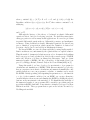
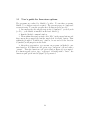
Using this method, we have developed a user-interface of programs for
calculations and simulations of BSDEs. With this user-interface people who
have no experience in stochastic calculations and numerical simulations could
quickly learn how to use our programs to calculate, to simulate and to study
the BSDEs. Briefly speaking, after inputting his parameters, i.e., the function
g = g(y, z), the terminal condition ξ in our BSDE, one can type them into
our user-interface then execute and simulate the BSDE by clicking the related
buttons on the user-interface shown in fig.1.1. We think that the visibility of
the numerical results of our programs will be useful for specialists and non
specialists in BSDE. Such knid of user-interface is firstly developped by Zhou
Haibin from 1996. These program that we put on the website are made by
Xu Mingyu from 2000.
2
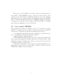
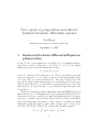
Non−linear g−expectation
yt =ξ + ∫Tt g(s, ys, zs)ds − ∫Tt zsdBs
t ∈ [0,T ], T = 1.
E g[ξ ] = y0
input g(t,y,z):
ξ = Φ(B(1)), input Φ(x) :
Figure 1:Interface for g-expectation(BSDE)
In fact this group of programs can be used to calculate the BSDE, not
only the g-expectation, since the g-expectation is a specialized BSDE with a
condition of g s.t. g(y, 0) ≡ 0 for ∀y ∈ R.
1.1
User’s guide for BSDE: g-expectations
The programs are realized by Matlab’s *.p files. To run these programs,
Matlab 5.3 or higher version is required. The present pagage is compressed
as gexp.zip. To run the progam, the following steps are needed:
1. uncompress the file gexp.zip in the document C: \matlab \work (or
D:\..., your Matlab is installed in the hard disk D:\).
2. Run the Matlab command window.
3. Then within this window single click “File” in the menu buttons and
then, among the prompted file buttons, single click “Set Path” button. Then
3
within the prompted “Path Browse” window, browse and add the direction
C:\matlab\work\gexp in the Path.
4. After these preparation, you can run our program: in Matlab’s command window, type “gexpectation” followed with a “return”. Then the g–
expectation window (figure No.1) is prompted.
An important feature of this program is its strong capacity of userinterface. Run command in the command window. We get the main userinterface shown in fig. 1.1.
At the left side of the user-interface, the g-expectation is shown on the
upside to indicate you the meaning of input functions. On the downside, you
can input two functions: the generator g and the terminal condition ξ. For
example, in fig.1.1 we will input: g(t, y, z) = −z 2 , ξ = Φ(B1 ) = sin(|B1 |). So
in the blank spaces we type g=-z.ˆ2, Φ=sin(abs(x)). Here we offer a table of
the transform between the formulas and the expressions in Matlab, the left
are the fomula in mathematics, the right are the expression in Matlab.
Multiply (×)
Divide (÷)
The power of n (xn )
Absolute value√(|x| )
Squrare root ( x)
Exponential (ex )
Natural logarithm (log x)
Sine (sin(x))
.*
./
x.ˆn
abs(x)
sqrt(x)
exp(x)
log(x)
sin(x)
The plus and minus are just + and -, respectively. And for the trigonometric
functions, the expressions are also like usual, so we did not list them out in
the table.
For the coefficient g, the function only depend on t, y, z. It can not support
other variable expect t, y, z. And for the terminal condition Φ, it’s same, Φ
only can have one variable x.
After inputting the parameters, you can use these programs to do the
calculation.
1. Clicking the button ’calculate’ on the left-side once, then the program
of calculation will run. For getting the result, calculation will take certain
seconds and then indicate the end of the calculation by jumping a dialoguebox “the calculation is complete.” .
2. Click the next button “progress”, the program will generate a new
figure, named ”calculating process of solution y”. On this figure, you will see
4
the backward computation procedure of the function y(t, x), dynamically and
backwardly. In the figure the red lines above (resp. blue lines below) show
the solution y (resp. Brownian motion). At the end, we can see a vertical
red line, which simify the value of solution y at time 0. Then the colorful
surface of solution y is generated in a new figure, which is named ”surface
for solution y”. The green lines in this figure show the relation between the
solution y and the Brownian motion, while the blue line below indicate the
range of descret Brownian motion. By clicking the button ”right”, ”up”, you
can see the surface in different direction.
The next three buttons on the main user-interface are for the simulations
of the solved (yt , zt ) .
3. Click the button “Brownian motion”, a dynamically generated Brownian path will appear on the new figure, ’Sample way of Brownian Motion’.
This path will terminated by a jump of a vertical line indicating the terminal
value yT = ξ(ω) of this sample. If you click the button “more” on this new
figure, then another Brownian path and the related ξ(ω) will be produced in
a different color.
4. Click the button “solution (y, z)” , you will see a moving (yt , zt ) on
the generated new figure ”trajetories of solution y ”. In the 1st (resp. the
2nd) column we show the trajetory of (Bt , yt ) (resp. (Bt , zt )). On the above
they are showed by a 3-d moving image, the red (resp. blue) lines show a
trajetory of the solution y (resp. Brownian motion), and the light red vertical
lines indicate the relation between the two trajetories. On the below, this
trajetory of solution y is showed in 2-d moving image by a red line, with
time being the x-coordinate. Clicking “more” button on this figure, there
will produce a different couple (yt , zt ) corresponding to a different Brownian
motion path. Like in the figure for the solution surface the button ”center”,
”right” and ”up” are for see the two 3-d image in different direction.
5. Clicking the following button ”B.M. and solution y”, you will get a
new figure, ”solution y on the surface”, for the sample way of solution y on
the solution surface. On the above window of it, a trajectory of Brownian
Motion Bt (ω) is showed on the ground, while the solution yt according to
this Brownian motion is showed on the solution surface. The button ”more”
is still for a new group of lines produced in the same color, and the button
”right”, ”up” are for the same use like the ones in the figure ”surface for
solution y”.
6. Click the next button ”distribution”, a new figure ”distribution function” is generated to show the distribution function of solution y at different
5
time t. On this figure, from the time T = 1 to t = 0, the distribution functions of solution y are showed by lines in different color by turn. The button
”right”, ”up” are for the same use.
7. For closing the figures there is two ways. One is using the button
”Close” on them. The other is to click the little cross on the right-up corner
of the figure.
In all the images,the meanings of the coordinate axises are noted directly
beside the corresponding axises. So we omit the detailed explanation.
2
2.1
Reflected Backward Stochastic Differential
Equations
Introduction for reflected backward differential equations
The reflected backward stochastic differential equations (RBSDE in short)
are firstly introduced by N. El Karoui, C. Kapodjian, E. Pardoux, S. Peng
and M.C. Quenez in [3]. We need the following notation,
(
)
2
S 2 [0, T ] = {ϕt , 0 ≤ t ≤ T } is a 1-d Ft -progressively processs.t.E( sup |ϕt | ) < +∞ .
0≤t≤T
n
o
Si2 [0, T ] = {ϕt , 0 ≤ t ≤ T } is a 1-d continuous increasing process s.t.E(|ϕT |2 ) < +∞
With assumptions: (i) a terminal condition ξ ∈ L2T ; (ii) a map g, which
satisfied g : [0, T ] × R × R → R, g(·, 0, 0) ∈ L2 ,and the Lipschitz condition:
∀(y1 , z1 ), (y2 , z2 ) ∈ R × Rd , there exists a constant C > 0, satisfying
|g(t, y1 , z1 ) − g(t, y2 , z2 )| ≤ C(|y1 − y2 | + |z1 − z2 |);
(iii) the lower barrier L, a Ft -adapted continuous process, s.t. E(sup0≤t≤T (Lt )2 ) <
+∞. The solution of RBSDE w.r.t. the lower barrier L is the triple (Y, Z, A) ∈
S 2 [0, T ] × H 2 [0, T ] × Si2 [0, T ], which satisfies
Yt = ξ +
Z T
t
g(r, Yr , Zr )dr + AT − At −
and Lt ≤ Yt for 0 ≤ t ≤ T ,
RT
0
(Yt − Lt )dAt = 0, a.s.
6
Z T
t
Zr dBr .
In the paper [3] of N. El Karoui et al, the existence and uniqueness for
the solution of such RBSDE is proved. Moreover, in the Section 6, they
consider a very clever method, penalization method to prove the existence.
This method also stir out the study for the numerical solution for RBSDE.
How to calculate the numerical solution for RBSDE is written in the paper
”Convergence of solutions of discrete reflected Backward SDE’s” by J.Memin
and S.Peng, the simulation is done by M.Xu [4].
2.2
User’s guide: RBSDEs
The programs are realized by Matlab’s *.p files. To run these programs,
Matlab 5.3 or higher version is required. The present pagage is compressed
as rebsde.zip. To run the progam, the following steps are needed:
1. uncompress the file rebsde.zip in the document C: \matlab\work (or
D:\..., your Matlab is installed in the hard disk D:\).
2. Run the Matlab command window.
3. Then within this window single click “File” in the menu buttons and
then, among the prompted file buttons, single click “Set Path” button. Then
within the prompted “Path Browse” window, browse and add the direction
C:\matlab\work\rebsde in the Path.
4. After these preparation, you can run our program: in Matlab’s command window, type “rebsde” followed with a “return”. Then the reflected
BSDE window (figure No.2) is prompted.
7
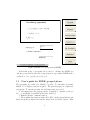
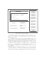
reflected BSDE
Yt = ξ + ∫Tt g(Ys ,Zs)ds + AT − At − ∫Tt ZsdBs
t ∈ [0,T ], T = 1.
Yt ≥ St ,
0≤t≤T
input g(y,z):
ξ = Φ(B(1)), input Φ(x) :
St = Ψ(t,B(t)), input Ψ(t,x) :
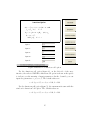
Figure 2:Interface reflected BSDE
An important feature of this program is its strong capacity of userinterface. Run command in the command window. We get the main userinterface shown in fig. 2.
At the left side of the user-interface, the reflected BSDE is shown on the
upside to indicate you the meaning of input functions. On the downside, you
can input three functions: the generator g, the terminal condition ξ, and the
barrier St . For example, in fig.1.2 we will input: g(t, y, z) = −10 |y + z| − 1,
ξ = Φ(B1 ) = |B1 |, St = Ψ(t, Bt ) = −3 × (B(t) − 1)2 + 1. So in the blank
spaces we type g=-10.*abs(y+z)-1, Φ=abs(x), Ψ(t,x)=-3.*(x-1).ˆ2+1. To
see the expression in Matlab, please read the tablet in Section 2.2, or use the
help in Matlab.
For the coefficient g, the function only depend on t, y, z. It can not support
other variable expect t, y, z. And for the terminal condition Φ, it’s same, Φ
only can have one variable x, which take place of the B1 . For the barrier Ψ,
8
it only has the variable t, x, t is for the time, x is for the Brownian motion
Bt .
After inputting the parameters, you can use these programs to do the
calculation.
1. Clicking the button ’calculate’ on the left-side once, then the program
of calculation will run. For getting the result, calculation will take certain
seconds and then indicate the end of the calculation by jumping a dialoguebox “the calculation is complete.” .
2. Click the next button “progress”, the program will generate a new
figure, named ”calculating process of solution y”. On this figure, you will
see the backward computation procedure of the function y(t, x), dynamically
and backwardly. In the figure the red lines above (resp. blue lines below)
show the solution y (resp. Brownian motion). The grid surface is the barrier.
At the end, we can see a vertical red line, which simify the value of solution y
at time 0. Then the above colorful surface of solution y is generated in a new
figure, which is named ”surface for solution y”. The green lines in this figure
show the relation between the solution y and the Brownian motion, while the
blue line below indicate the range of descret Brownian motion. By clicking
the button ”right”, ”up”, you can see the surface in different direction.
The next three buttons on the main user-interface are for the simulations
of the solved (yt , zt ) .
3. Click the button “Brownian motion”, a dynamically generated Brownian path will appear on the new figure, ’Sample way of Brownian Motion’.
This path will terminated by a jump of a vertical line indicating the terminal
value yT = ξ(ω) of this sample. If you click the button “more” on this new
figure, then another Brownian path and the related ξ(ω) will be produced in
a different color.
4. Click the button “solution (y, z)” , you will see a moving (yt , zt , At )
on the generated new figure ”trajetories of solution y and z and A ”. In the
1st (resp. the 2nd) column we show the trajetory of (Bt , yt ) (resp. (Bt , zt )).
On the above they are showed by a 3-d moving image, the red (resp. blue)
lines show a trajetory of the solution y (resp. Brownian motion), and the
light red vertical lines indicate the relation between the two trajetories. On
the below, this trajetory of solution y is showed in 2-d moving image by a
red line, with time being the x-coordinate. In the above of the 3rd column,
the ’push’ At corresponding to the solution yt is shown. And in the below
of the 3rd column, it’s the difference of the yt and St , i.e. yt − St . Clicking
“more” button on this figure, there will produce a different triple (yt , zt , At )
9
corresponding to a different Brownian motion path. Like in the figure for the
solution surface the button ”center”, ”right” and ”up” are for see the two
3-d image in different direction.
5. Clicking the following button ”B.M. and solution y”, you will get a
new figure, ”solution y on the surface”, for the sample way of solution y on
the solution surface. On the above window of it, a trajectory of Brownian
Motion Bt (ω) is showed on the ground, while the solution yt according to this
Brownian motion is showed on the solution surface. And the grey surface is
for the barrier St . On the below windows, there are the trajectories of At
(on the left) and yt − St (on the right). The button ”more” is still for a new
group of lines produced in the different color, and the button ”right”, ”up”
are for the same use like the ones in the figure ”surface for solution y”.
6. Click the next button ”distribution”, a new figure ”distribution function” is generated to show the distribution function of solution y at different
time t. On this figure, from the time T = 1 to t = 0, the distribution functions of solution y are showed by lines in different color by turn. The button
”right”, ”up” are for the same use.
7. For closing the figures there is two ways. One is using the button
”Close” on them. The other is to click the little cross on the right-up corner
of the figure.
In all the images,the meanings of the coordinate axises are noted directly
beside the corresponding axises. So we omit the detailed explanation.
2.3
User’s guide: the penalization BSDEs for RBSDEs
For an RBSDE with the parameters (ξ, g, L) satisfying the assumptions (i)(iii) in section 2.1, denote (Y p , Z p ) ∈ S 2 [0, T ] × H 2 [0, T ] (for each p ∈ N )
be the unique pair of Ft -progressively processes satisfying
Ytp = ξ +
Z T
t
g(r, Yrp , Zrp )dr + p
Z T
R
t
(Yrp − Sr )− dr −
Z T
t
Zrp dBr ,
and let Apt = 0T (Yrp −Sr )− dr. Such equation is called the penalization BSDEs
w.r.t. (ξ, g, L).
In [3] N.El Karoui et al. Section 6, we know that the solution (Y p , Z p , Ap )
of the penalization BSDEs converges to the solution (Y, Z, A) of RBSDE in
the space S 2 [0, T ] × H 2 [0, T ] × Si2 [0, T ]. Then we use the numerical method
for BSDEs to calculate the penalization BSDEs.
10
The programs are realized by Matlab’s *.p files. To run these programs,
Matlab 5.3 or higher version is required. The present pagage is compressed
as pebsde.zip. To run the progam, the following steps are needed:
1. uncompress the file rebsde.zip in the document C: \matlab\work (or
D:\..., your Matlab is installed in the hard disk D:\).
2. Run the Matlab command window.
3. Then within this window single click “File” in the menu buttons and
then, among the prompted file buttons, single click “Set Path” button. Then
within the prompted “Path Browse” window, browse and add the direction
C:\matlab\work\pebsde in the Path.
4. After these preparation, you can run our program: in Matlab’s command window, type “pebsde” followed with a “return”. Then the penalization BSDE window (figure No.3) is prompted.
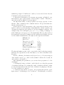
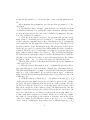
BSDE under Penalization
ytp = ξ + ∫Tt [g(t,ysp ,zsp)+ p⋅(ytp− St)−]ds − ∫Tt zspdBs
t ∈ [0,T ], T = 1.
ytp → Yt , p → ∞
input g(t,y,z):
ξ = Φ(B(1)), input Φ(x) :
input p :
St = Ψ(t,B(t)), input Ψ(t,x) :
Figure 3:Interface penalization BSDE
11
At the left side of the user-interface, the penalization BSDE is shown on
the upside to indicate you the meaning of input functions. On the downside,
you can input three functions: the generator g, the penalization’s parameter
p, the terminal condition ξ, and the barrier St . For example, in fig.1.2 we will
input: g(t, y, z) = −10 |y + z| − 1, ξ = Φ(B1 ) = |B1 |, p = 10, St = Ψ(t, Bt ) =
−3 × (B(t) − 1)2 + 1. So in the blank spaces we type g=-10.*abs(y+z)-1,
Φ=abs(x), p=10, Ψ(t,x)=-3.*(x-1).ˆ2+1. To see the expression in Matlab,
please read the tablet in Section 2.2, or use the help in Matlab.
For the coefficient g, the function only depend on t, y, z. It can not support
other variable expect t, y, z. And for the terminal condition Φ, it’s same, Φ
only can have one variable x, which take place of the B1 . For the barrier Ψ,
it only has the variable t, x, t is for the time, x is for the Brownian motion
Bt .
After inputting the parameters, you can use these programs to do the
calculation. On this figure the functions of the buttons on the right side are
almost same with the ones on the figure for ’RBSDE’. You can find the detail
explanation in the Section 2.2.
1. The button ’calculate’ is for calculation.
2. The button “progress” is for show the procedure of the function
p
y (t, x), dynamically and backwardly.
The next three buttons on the main user-interface are for the simulations
of the solved (ytp , ztp ) .
3. The button “Brownian motion” is for a dynamically generated Brownian with the terminal value yTp = ξ(ω) of this sample.
4. The button “solution (y, z)” , is for trajetories of solution y p and z p .
Same as the one on the figure ”g-expectation”.
5. The button ”B.M. and solution y” is for the sample way of solution y p
on the solution surface. The differences with the Rbutton ”B.M. and solution
y” is the window below, this window is for Apt = 0T (Yrp − Sr )− dr.
6. The next button ”difference” is to show the difference between the
numerical solution of penelization BSDE and reflected BSDE. After load the
data of penalization BSDE and reflected BSDE, first, the program will check
if the parametres g, ξ, S, of the two equations are same, if they are not same
a dialogue window will be generated ”CANNOT COMPARE! The function
or terminal condition or obstacle is defferent!”. If they are same, a new
figure named ”the difference of PBSDE and RBSDE” will be shown, with
the surface of the difference. The button ”right”, ”up” are for the same use.
7. For closing the figures there is two ways. One is using the button
12
”Close” on them. The other is to click the little cross on the right-up corner
of the figure.
In all the images,the meanings of the coordinate axises are noted directly
beside the corresponding axises. So we omit the detailed explanation.
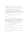
3
Applications to American options
Now we will discuss some applications of the reflected BSDE. In the mathematical finance, we know that American option can be described by the
linear reflected BSDE. For the American call option, the wealth yt satisfies
the following BSDE
yt = (xT − k)+ −
xt = x0 +
Z t
0
Z T
t
[rys + (µ − r)zs ]ds −
µxs ds +
Z t
0
Z T
t
σzs dBs , 0 ≤ t ≤ 1
σxs dBs ,
and yt satisfies
yt ≥ St , for 0 ≤ t ≤ τ, where St = (xt − k)+ ,
where τ is a stopping time, and τ = inf{t, yt − St < 0}. In finance, yt is
wealth process, xt is price of stock, τ stand for exit time from market for the
investor. At this time he will do the action buying or selling the stock. In
this problem, we are interested in the yt , zt , and τ. To solve it, we consider
it as a reflected BSDE, with the barrier St , then τ = inf{t, At > 0}.
Reflected BSDE applied to American put option corresponds to the case:
yT = ξ = (k − xT )+ , St = (k − xt )+ .
The investor’s wealth yt satisfies the RBSDE:
yt = (k − xT )+ −
yt ≥ St , dAt ≥ 0,
Z T
t
[rys + (µ − r)zs ]ds + AT − At −
Z T
0
Z T
t
zs dBs , 0 ≤ t ≤ 1
(yt − St )dAt = 0,
where xt is the price of the underlying stock which is a geometric Brownian
motion:
Z t
Z t
xt = x0 +
µxs ds +
σxs dBs .
0
0
At the stopping time τ = inf{t, At > 0}. The investor will execute the
contract and his return is (k − xτ )+ .
13
3.1
User’s guide for American options.
The programs are realized by Matlab’s *.p files. To run these programs,
Matlab 5.3 or higher version is required. The present pagage is compressed
as amoption.zip. To run the progam, the following steps are needed:
1. uncompress the file amoption.zip in the document C: \matlab\work
(or D:\..., your Matlab is installed in the hard disk D:\).
2. Run the Matlab command window.
3. Then within this window single click “File” in the menu buttons and
then, among the prompted file buttons, single click “Set Path” button. Then
within the prompted “Path Browse” window, browse and add the direction
C:\matlab\work\amoption in the Path.
4. After these preparation, you can run our program: in Matlab’s command window. For American call option, type “amoption” followed with a
“return”. Then the American call option window (figure 4) is prompted.
For American pull option, type ”aoptionpu” following with a ”enter”, the
American pull option window (figure 5) is generated.
14
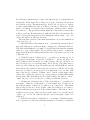
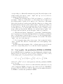
American Option
−dyt = − [r⋅ yt + (µ − r)⋅ zt]dt − σ ⋅ ztdBt
yT = ( xT − k )+,
T = 1.
dxt = µ ⋅ xt dt + σ ⋅ xt dBt ,
St = ( xt − k
x(0) = x0.
)+.
and Yt ≥ St ,
0≤t≤τ
input r :
input µ :
input σ :
input x0 :
input k :
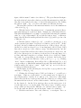
Figure 4:Interface for American call option
For the American call option (figure 4), on the left side of the userinterface, the reflected BSDE for American call option is shown on the upside
to indicate you the meaning of input parametres. On the downside, you can
input the parametres: r, µ, σ, x0 , k, The default values are
r = 0.1, µ = 0.5, σ = 1, x0 = 100, k = 100.
For the American pull option (figure 5), the arranement is same with the
window for American call option. The default values are
r = 0.1, µ = 0.5, σ = 1, x0 = 100, k = 100.
15
American Option
−dyt = − [r⋅ yt + (µ − r)⋅ zt]dt − σ ⋅ ztdBt
yT = ( k − xT )+,
T = 1.
dxt = µ ⋅ xt dt + σ ⋅ xt dBt , x(0) = x0.
St = ( k − xt )+.
and Yt ≥ St ,
0≤t≤τ
input r :
input µ :
input σ :
input x0 :
input k :
Figure 5:Interface for American pull option
After inputting the parameters, you can use these programs to do the
calculation. The functions of the buttons on the windows for American call
or pull option are same. So we write their fnctions together.
1. Clicking the button ’calculate’ on the left-side once, then the program
of calculation will run. For getting the result, calculation will take certain
seconds and then indicate the end of the calculation by jumping a dialoguebox “the calculation is complete.” .
2. Click the next button “progress”, the program will generate a new
figure, named ”calculating process of solution y”. On this figure, you will
see the backward computation procedure of the function y(t, x), dynamically
and backwardly. In the figure the red lines above (resp. blue lines below)
show the solution y (resp. Brownian motion). The grid surface is the barrier.
At the end, we can see a vertical red line, which simify the value of solution y
at time 0. Then the above colorful surface of solution y is generated in a new
16
figure, which is named ”surface for solution y”. The green lines in this figure
show the relation between the solution y and the Brownian motion, while the
blue line below indicate the range of descret Brownian motion. By clicking
the button ”right”, ”up”, you can see the surface in different direction.
The next three buttons on the main user-interface are for the simulations
of the solved (yt , zt ) .
3. Click the button “Brownian motion”, a dynamically generated Brownian path will appear on the new figure, ’Sample way of Brownian Motion’.
This path will terminated by a jump of a vertical line indicating the terminal
value yT = ξ(ω) of this sample. If you click the button “more” on this new
figure, then another Brownian path and the related ξ(ω) will be produced in
a different color.
4. Click the button “solution (y, z, A)” , you will see a moving (yt , zt , At )
on the generated new figure ”trajetories of solution y and z and A ”. In the
1st (resp. the 2nd) column we show the trajetory of (Bt , yt ) (resp. (Bt , zt )).
On the above they are showed by a 3-d moving image, the red (resp. blue)
lines show a trajetory of the solution y (resp. Brownian motion), and the
light red vertical lines indicate the relation between the two trajetories. On
the below, this trajetory of solution y is showed in 2-d moving image by a
red line, with time being the x-coordinate. In the above of the 3rd column,
the ’push’ At corresponding to the solution yt is shown. And in the below
of the 3rd column, it’s the difference of the yt and St , i.e. yt − St . Clicking
“more” button on this figure, there will produce a different triple (yt , zt , At )
corresponding to a different Brownian motion path. Like in the figure for the
solution surface the button ”center”, ”right” and ”up” are for see the two
3-d image in different direction.
On this figure and the following two, the big blue or grey point is for the
exit time τ = inf{t, At > 0}.
5. Clicking the following button ”B.M. and solution y”, you will get a
new figure, ”solution y on the surface”, for the sample way of solution y on
the solution surface. On the above window of it, a trajectory of Brownian
Motion Bt (ω) is showed on the ground, while the solution yt according to this
Brownian motion is showed on the solution surface. And the grey surface is
for the barrier St . On the below windows, there are the trajectories of At
(on the left) and yt − St (on the right). The button ”more” is still for a new
group of lines produced in the different color, and the button ”right”, ”up”
are for the same use like the ones in the figure ”surface for solution y”.
6. Click the next button ”Price and solution y”, a new figure ”Price on
17
the result surface” is generated. This figure is almost same as the figure
”solution y on the surface”, expect that on the 3-d window the price of the
stock Xt take the place of the Brownian motion Bt . The button ”right”, ”up”
are for the same use.
7. For closing the figures there is two ways. One is using the button
”Close” on them. The other is to click the little cross on the right-up corner
of the figure.
In all the images,the meanings of the coordinate axises are noted directly
beside the corresponding axises. So we omit the detailed explanation.
Note: If you have any suggestion for this user’s guide or for the programs,
please contact me: [email protected]
References
[1] P.Briand, B. Delyon, J. M´emin. Donsker-type theorem for BSDEs, Elect.
Comm. in Probab. 6 (2001) 1-14.
[2] J. M. Bismut (1973): “Conjugate Convex Functions in Optimal Stochastic Control,” J.Math. Anal. Apl., 44, pp.384-404.27.
[3] N. El Karoui, C. Kapoudjian, E. Pardoux, S. Peng and M.-C. Quenez
(1997), Reflected Solutions of Backward SDE and Related Obstacle Problems for PDEs, Ann. Probab. 25, no 2, 702–737.
[4] J.M´emin, S.Peng, (simulatiob by M.Xu) (2002) Convergence of solutions
of discret reflected backward SDE’s, preprint.
[5] E. Pardoux and S. Peng. Adapted solutions of Backward Stochastic Differential Equations. Systems Control Lett. 14 (1990), 51-61.
18