Download User's guide of reflected BSDE with two barriers and other topic

User’s guide of reflected BSDE with two
barriers and other topic
Mingyu XU
a School
a,b∗
of Mathematics and System Science, Shandong University,
250100, Jinan, China
b Department
of Financial Mathematics and Control science, School of Mathematical Science,
Fudan University, Shanghai, 200433, China.
c Institute
1
of Applied Mathematics, AMSS, CAS, 100190, Beijing, China
Reflected Backward Stochastic Differential
Equations
1.1
Introduction for reflected backward differential equations with one or two barriers
The reflected backward stochastic differential equations (RBSDE in short)
are firstly introduced by N. El Karoui, C. Kapodjian, E. Pardoux, S. Peng
and M.C. Quenez in [4]. We need the following notation,
(
)
2
2
S [0, T ] = {ϕt , 0 ≤ t ≤ T } is a 1-d Ft -progressively processs.t.E( sup |ϕt | ) < +∞ .
0≤t≤T
n
o
Si2 [0, T ] = {ϕt , 0 ≤ t ≤ T } is a 1-d continuous increasing process s.t.E(|ϕT |2 ) < +∞
With assumptions: (i) a terminal condition ξ ∈ L2T ; (ii) a map g, which
satisfied g : [0, T ] × R × R → R, g(·, 0, 0) ∈ L2 ,and the Lipschitz condition:
∀(y1 , z1 ), (y2 , z2 ) ∈ R × Rd , there exists a constant C > 0, satisfying
|g(t, y1 , z1 ) − g(t, y2 , z2 )| ≤ C(|y1 − y2 | + |z1 − z2 |);
∗
Email: [email protected]
1
(iii) the lower barrier L, upper barrier U , which are Ft -adapted continu− 2
2
ous processes, s.t. E(sup0≤t≤T (L+
t ) ) + E(sup0≤t≤T (Ut ) ) < +∞. And we
assume there exists a semimartingale, such that Lt ≤ Xt ≤ Ut .
The solution of RBSDE w.r.t. the lower barrier L is the triple (Y, Z, A) ∈
S 2 [0, T ] × H 2 [0, T ] × Si2 [0, T ], which satisfies
Z
Yt = ξ +
t
T
Z
g(r, Yr , Zr )dr + AT − At −
T
Zr dBr .
t
R
and Lt ≤ Yt for 0 ≤ t ≤ T , 0T (Yt − Lt )dAt = 0, a.s.
The solution of RBSDE w.r.t. the lower barrier L and upper barrier U is
the triple (Y, Z, A, K) ∈ S 2 [0, T ] × H 2 [0, T ] × Si2 [0, T ], which satisfies
Z
Yt = ξ +
t
T
Z
g(r, Yr , Zr )dr + AT − At − (KT − Kt ) −
R
t
T
Zr dBr .
R
and Lt ≤ Yt ≤ Ut for 0 ≤ t ≤ T , 0T (Yt − Lt )dAt = 0T (Yt − Ut )dKt = 0, a.s.
And we also have
programR to simulation reflected BSDE with a diffusion
R
process Xt = x + 0t bXs ds + 0t σXs dBs . The reflect BSDE is as following
Z
Yt = ξ +
t
T
Z
H(r, Xr Yr , Zr )dr + AT − At −
t
T
Zr dBr
R
and Lt ≤ Yt for 0 ≤ t ≤ T , 0T (Yt − Lt )dAt = 0, a.s.
In the paper [4] of N. El Karoui et al, the existence and uniqueness for
the solution of such RBSDE is proved. Moreover, in the Section 6, they
consider a very clever method, penalization method to prove the existence.
This method also stir out the study for the numerical solution for RBSDE.
How to calculate the numerical solution for RBSDE is written in the paper
”Convergence of solutions of discrete reflected Backward SDE’s” by J.Memin
and S.Peng, the simulation is done by M.Xu [6].
1.2
User’s guide: Reflected BSDEs with two barriers
The programs are realized by Matlab’s *.p files. To run these programs,
Matlab 5.3 or higher version is required. The present package is compressed
as rebsdetb.zip. After download the compressed file, you should:
1. uncompress the file rebsde.zip in the document C: \matlab\work (or
D:\..., your Matlab is installed in the hard disk D:\).
2. Run the Matlab command window.
2
3. Then within this window single click “File” in the menu buttons and
then, among the prompted file buttons, single click “Set Path” button. Then
within the prompted “Path Browse” window, browse and add the direction
C:\matlab\work\rebsdetb in the Path.
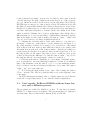
4. After these preparation, you can run our program: in Matlab’s command window, type “rebsdetb” followed with a “return”. Then the reflected
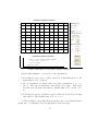
BSDE window (figure No.3) is prompted.
reflected BSDE
Yt = ξ + ∫Tt g(s,Ys ,Zs)ds + AT − At− (KT − Kt)
− ∫Tt ZsdBs
t ∈ [0,T ], T = 1.
Lt ≤ Yt ≤ Ut ,
0≤t≤T
∫T0 (Yt − Lt )dAt = 0, ∫T0 (Yt − Ut )dKt = 0
input g(t,y,z):
ξ = Φ(B(1)), input Φ(x) :
Lt = Ψ1(t,B(t)), input Ψ1(t,x) :
U = Ψ2(t,B(t)), input Ψ2(t,x):
t
Figure 3:Interface reflected BSDE
An important feature of this program is its strong capacity of userinterface. Run command in the command window. We get the main userinterface shown in fig. 2.
At the left side of the user-interface, the reflected BSDE is shown on the
upside to indicate you the meaning of input functions. On the downside, you
can input three functions: the generator g, the terminal condition ξ, and the
3
barrier St . For example, in fig.1.2 we will input: g(t, y, z) = −10 |y + z| − 1,
ξ = Φ(B1 ) = |B1 |, Lt = Ψ1 (t, Bt ) = −3 × (B(t) − 2)2 + 3, Ut = Ψ2 (t, Bt ) =
(B(t) + 1)2 + 3(t − 1). So in the blank spaces we type g=-10.*abs(y+z)1, Φ=abs(x), Ψ1 (t,x)=-3.*(x-2).ˆ2+3, Ψ2 (t,x)=(x+1).ˆ2+3(t-1). To see the
expression in Matlab, please read the tablet in Section 2.2, or use the help
in Matlab.
For the coefficient g, the function only depend on t, y, z. It can not support
other variable expect t, y, z. And for the terminal condition Φ, it’s same, Φ
only can have one variable x, which take place of the B1 . For the barrier
Ψ1 , Ψ2 , it only has the variable t, x, t is for the time, x is for the Brownian
motion Bt .
After inputting the parameters, you can use these programs to do the
calculation.
1. Clicking the button ’calculate’ on the left-side once, then the program
of calculation will run. For getting the result, calculation will take certain
seconds and then indicate the end of the calculation by jumping a dialoguebox “the calculation is complete.” .
2. Click the next button “progress”, the program will generate a new
figure, named ”calculating process of solution y”. On this figure, you will
see the backward computation procedure of the function y(t, x), dynamically
and backwardly. In the figure the red lines above (resp. blue lines below)
show the solution y (resp. Brownian motion). The grid surface is the barrier.
At the end, we can see a vertical red line, which simplify the value of solution
y at time 0. Then the above colorful surface of solution y is generated in a
new figure, which is named ”surface for solution y”. The green lines in this
figure show the relation between the solution y and the Brownian motion,
while the blue line below indicate the range of descrete Brownian motion.
By clicking the button ”right”, ”up”, you can see the surface in different
direction.
The next three buttons on the main user-interface are for the simulations
of the solved (yt , zt ) .
3. Click the button “Brownian motion”, a dynamically generated Brownian path will appear on the new figure, ’Sample way of Brownian Motion’.
This path will terminated by a jump of a vertical line indicating the terminal
value yT = ξ(ω) of this sample. If you click the button “more” on this new
figure, then another Brownian path and the related ξ(ω) will be produced in
a different color.
4. Click the button “solution (y, z, A, K)” , you will see a moving (yt , zt , At , Kt )
4
on the generated new figure ”trajectories of solution y and z and A and K
”. In the 1st (resp. the 2nd) column we show the trajectory of (Bt , yt ) (resp.
(Bt , zt )). On the above they are showed by a 3-d moving image, the red (resp.
blue) lines show a trajectory of the solution y (resp. Brownian motion), and
the light red vertical lines indicate the relation between the two trajectories.
On the below, this trajectory of solution y is showed in 2-d moving image by
a red line, with time being the x-coordinate. In the 3rd column, we show the
’push’ At and Kt . Clicking “more” button on this figure, there will produce a
different triple (yt , zt , At ) corresponding to a different Brownian motion path.
Like in the figure for the solution surface the button ”center”, ”right” and
”up” are for see the two 3-d image in different direction.
5. Clicking the following button ”B.M. and solution y”, you will get a
new figure, ”solution y on the surface”, for the sample way of solution y on
the solution surface. On the above window of it, a trajectory of Brownian
Motion Bt (ω) is showed on the ground, while the solution yt according to this
Brownian motion is showed on the solution surface. And the grey surface is
for the barrier St . On the below windows, there are the trajectories of At (on
the left) and Kt (on the right). The button ”more” is still for a new group
of lines produced in the different color, and the button ”right”, ”up” are for
the same use like the ones in the figure ”surface for solution y”.
6. Click the next button ”distribution”, a new figure ”distribution function” is generated to show the distribution function of solution y at different
time t. On this figure, from the time T = 1 to t = 0, the distribution functions of solution y are showed by lines in different color by turn. The button
”right”, ”up” are for the same use.
7. For closing the figures there is two ways. One is using the button
”Close” on them. The other is to click the little cross on the right-up corner
of the figure.
In all the images,the meanings of the coordinate axises are noted directly
beside the corresponding axises. So we omit the detailed explanation.
1.3
User’s guide: Reflected BSDEs with one lower barrier and a diffusion process
The programs are realized by Matlab’s *.p files. To run these programs,
Matlab 5.3 or higher version is required. The present package is compressed
as rebsdex.zip. After download the compressed file, you should:
5
1. uncompress the file rebsde.zip in the document C: \matlab\work (or
D:\..., your Matlab is installed in the hard disk D:\).
2. Run the Matlab command window.
3. Then within this window single click “File” in the menu buttons and
then, among the prompted file buttons, single click “Set Path” button. Then
within the prompted “Path Browse” window, browse and add the direction
C:\matlab\work\rebsdex in the Path.
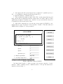
4. After these preparation, you can run our program: in Matlab’s command window, type “rebsdex2” followed with a “return”. Then the reflected
BSDE window (figure No.4) is prompted.
reflected BSDE
Xt = X0 + ∫t0 b Xs ds + ∫t0 σ XsdBs
Yt = ξ + ∫Tt H(s, Xs, Ys, Zs)ds + AT − At
− ∫Tt ZsdBs.
t ∈ [0,T ], T = 1.
Yt ≥ Lt , 0 ≤ t ≤ T.
input X0:
input b:
input σ:
input H(t,x,y,z):
ξ = Φ(B(1)), input Φ(B) :
L = Ψ(t,X(t)), input Ψ(t,x) :
t
Figure 4:Interface reflected BSDE
An important feature of this program is its strong capacity of userinterface. Run command in the command window. We get the main userinterface shown in fig. 2.
6
At the left side of the user-interface, the reflected BSDE is shown on the
upside to indicate you the meaning of input functions. On the downside, you
can input three functions: the generator g, the terminal condition ξ, and the
barrier St . For example, in fig.1.2 we will input: X0 = 1, b = 1, σ = 1,
H(t, x, y, z) = −x, ξ = exp(0.5 + BT ), Lt = 12 Xt . So in the blank spaces
we type g=-x, Φ=exp(.5+B), Ψ(t,x)=x./2. To see the expression in Matlab,
please read the tablet in Section 2.2, or use the help in Matlab.
For the coefficient H, the function only depend on t, x, y, z. It can not
support other variable expect t, x, y, z. And for the terminal condition Φ, it’s
same, Φ only can have one variable x, which take place of the B1 . For the
barrier Ψ, it only has the variable t, x, t is for the time, x is for the Brownian
motion Bt .
After inputting the parameters, you can use these programs to do the
calculation.
1. Clicking the button ’calculate’ on the left-side once, then the program
of calculation will run. For getting the result, calculation will take certain
seconds and then indicate the end of the calculation by jumping a dialoguebox “the calculation is complete.” .
2. Click the next button “progress”, the program will generate a new
figure, named ”calculating process of solution y”. On this figure, you will
see the backward computation procedure of the function y(t, x), dynamically
and backwardly. In the figure the red lines above (resp. blue lines below)
show the solution y (resp. Brownian motion). The grid surface is the barrier.
At the end, we can see a vertical red line, which simplify the value of solution
y at time 0. Then the above colorful surface of solution y is generated in a
new figure, which is named ”surface for solution y”. The green lines in this
figure show the relation between the solution y and the Brownian motion,
while the blue line below indicate the range of descrete Brownian motion.
By clicking the button ”right”, ”up”, you can see the surface in different
direction.
The next three buttons on the main user-interface are for the simulations
of the solved (yt , zt ) .
3. Click the button “solution y”, you will see a moving (yt ) on the generated new figure in 2-dimensional. Clicking “more” button on this figure,
there will produce a different triple (yt ) corresponding to a different Brownian
motion path.
4. Click the button “solution z”, you will see a moving (zt ) on the generated new figure in 2-dimensional. Clicking “more” button on this figure,
7
there will produce a different triple (zt ) corresponding to a different Brownian
motion path.
5. Click the button “solution (y,z)”, you will see a moving (yt , zt ) on
the generated new figure in 2-dimensional. and 3-dimensional. This left two
subfigures are for yt , while the right two are for zt . Clicking “more” button
on this figure, there will produce a different triple (yt , zt ) corresponding to a
different Brownian motion path.
6. Click the button “solution (y, z, A)” , you will see a moving (yt , zt , At )
on the generated new figure ”trajectories of solution y and z and A and K
”. In the 1st (resp. the 2nd) column we show the trajetory of (Bt , yt ) (resp.
(Bt , zt )). On the above they are showed by a 3-d moving image, the red (resp.
blue) lines show a trajectory of the solution y (resp. Brownian motion), and
the light red vertical lines indicate the relation between the two trajetories.
On the below, this trajectory of solution y is showed in 2-d moving image
by a red line, with time being the x-coordinate. In the 3rd column, we show
the ’push’ At and yt − Lt . Clicking “more” button on this figure, there will
produce a different triple (yt , zt , At ) corresponding to a different Brownian
motion path. Like in the figure for the solution surface the button ”center”,
”right” and ”up” are for see the two 3-d image in different direction.
7. Clicking the following button ”B.M. and solution y”, you will get a
new figure, ”solution y on the surface”, for the sample way of solution y on
the solution surface. On the above window of it, a trajectory of Brownian
Motion Bt (ω) is showed on the ground, while the solution yt according to this
Brownian motion is showed on the solution surface. And the grey surface is
for the barrier Lt . On the below windows, there are the trajectories of At
(on the left) and yt − Lt (on the right). The button ”more” is still for a new
group of lines produced in the different color, and the button ”right”, ”up”
are for the same use like the ones in the figure ”surface for solution y”.
8. For closing the figures there is two ways. One is using the button
”Close” on them. The other is to click the little cross on the right-up corner
of the figure.
In all the images,the meanings of the coordinate axises are noted directly
beside the corresponding axises. So we omit the detailed explanation.
8
2
Stochastic Hamilton system
Stochastic Hamilton system is a linear forward backward stochastic differential equation. See more details in [8].
dxt = [H21 xt + ρH22 yt + ρH23 zt ]dt + [ρH31 xt + ρH32 yt + H33 zt ]dBt
−dyt = [H1xt + H12 yt + ρH13 zt ]dt − zt dBt
x(0) = 0, y(T ) = 0.
Obviously (xt , yt , zt ) = (0, 0, 0) is its solution. We study its nonzero solution. ρ is eigenvalue of this system, which permits this FBSDE has nonzero
2
solution. And ρ satisfies ρH22 − H33 H13
≤ 0.
The programs are realized by Matlab’s *.p files. To run these programs,
Matlab 5.3 or higher version is required. The present package is compressed
as hamilton.zip. After download the compressed file, you should:
1. uncompress the file Xuamoption.zip in the document C: \matlab\work
(or D:\..., your Matlab is installed in the hard disk D:\).
2. Run the Matlab command window.
3. Then within this window single click “File” in the menu buttons and
then, among the prompted file buttons, single click “Set Path” button. Then
within the prompted “Path Browse” window, browse and add the direction
C:\matlab\work\hamilton in the Path.
4. After these preparation, you can run our program: in Matlab’s command window. For Stochastic Hamilton system, type “shamilton” followed
with a “return”. (figure 7) is generated.
9
Stochstic Hamiltonian systems
1
input H=
0.9
0.8
0.7
0.6
range:
0
0.5
9
0.4
input ρ , such that
0.3
2
ρ⋅ H22 − H33⋅H13≤ 0
0.2
0.1
0
0
0.1
0.2
0.3
0.4
0.5
0.6
0.7
0.8
0.9
1
Stochstic Hamiltonian systems
dxt= [H21xt+ ρH22yt+ ρH23zt ]dt+ [ρH31xt+ ρH32yt+H33zt ]dBt,
Curves depend on H
12
−dyt= [H11xt+H12yt+ρH13zt ]dt − ztdBt,
x (0 )=0 , y (T )=0.
Figure 7:Interface for Stochastic Hamilton System
On the right subfigure, you can choose the parameters:

• Hamilton matrix H, with H21

1
−0.5 1

1 
= −H12 , whose default value is  0.5 −2
;
1
1
−1
• range is for choosing time interval, which can be decided by slide bar;
2
• default eigenvalue ρ = 4, and it satisfies ρH22 − H33 H13
≤ 0.
5. Click ’Ricatti Curve’, the a pair of solution of Ricatti equation is show
in left upper portion, by blue and green line.
6. Click ’Stochastic Hamilton’, in left upper portion, a pair of strategies
of solution (xt , yt ) will be drawn by red and blue lines.
7. Click ’Curves’, user will see several pairs of strategies of solution
(xt , yt ), basing on same Brownian motion strategy, with parameter H12 changes
10
from −0.5 to 0 with each step 0.05. At last program will generate two new
figures to draw these in 3-dimensional.
7. For closing the figures there is two ways. One is using the button
”Close” on them. The other is to click the little cross on the right-up corner
of the figure.
2.1
Stochastic Laplace Transform
Stochastic Laplace transform is a kind of BSDE. For process ft , stochastic
Laplace transform of f is L[f ](s, µ) = p(0), where (p(t), q(t)) is the solution
of following complex valued BSDE on infinite interval [0, +∞):
−dp(t) = [−sp(t) + µ(t)q(t) + f (t)]dt − q(t)dW (t),
µ(t) = a × 1[0,T ] (t),
t ∈ [0, +∞), s ∈ C, µ(·) ∈ S.
The programs are realized by Matlab’s *.p files. To run these programs,
Matlab 5.3 or higher version is required. The present package is compressed
as hamilton.zip. After download the compressed file, you should:
1. uncompress the file Xuamoption.zip in the document C: \matlab\work
(or D:\..., your Matlab is installed in the hard disk D:\).
2. Run the Matlab command window.
3. Then within this window single click “File” in the menu buttons and
then, among the prompted file buttons, single click “Set Path” button. Then
within the prompted “Path Browse” window, browse and add the direction
C:\matlab\work\laplace in the Path.
4. After these preparation, you can run our program: in Matlab’s command window. For Stochastic Laplace transform, type “slaplace” followed
with a “return”. (figure 8) is generated.
11
Stochastic Laplace Transform
1
stochastic process :
0.9
f(t)= ψ(Wt)
input ψ (x) :
0.8
0.7
choose the parameter :
0.6
0.5
from
0.4
to
0.3
the defual parameter :
0.2
s=
0.1
0
T=
a=
0
0.1
0.2
0.3
0.4
0.5
0.6
0.7
0.8
0.9
1
Stochastic Laplace Transform
−dp(t) = [− s p(t) + µ(t) q(t)+ f(t)]dt − q(t)dW (t),
t ∈ [0, ∞) , s∈C , µ( ⋅ )∈S
µ(t) = a × 1
(t)
[0,T]
L[ f ]( s ,µ) = p (0)
Figure 8:Interface for Stochastic Laplace transform
On the right subfigure, you can choose the parameters:
• Stochastic process: f (t) = ψ(Wt ), where W is Brownian motion. Default value is ψ(x) = exp(x).
• Choose parameter by menu, there are three parameters s, T , a to
choose. The chosen parameter will change in a range. This range
is decided by following edit window, default value is for s from −2i to
2i.
• Following are rest two parameter, whose values are decided by following
edit window. The default value is T = 6, a = 1.
5. Click ’calculate’, program will generate the curve of stochastic Laplace
transform of f changing on chosen parameter in chosen range.
12
6. Click ’add line’, program will generate the curve of stochastic Laplace
transform of f in another color changing on same parameter in same range,
after user change any value of default parameters.
7. For closing the figures there is two ways. One is using the button
”Close” on them. The other is to click the little cross on the right-up corner
of the figure.
In all the images,the meanings of the coordinate axises are noted directly
beside the corresponding axises. So we omit the detailed explanation.
References
[1] P.Briand, B. Delyon, J. M´emin. Donsker-type theorem for BSDEs, Elect.
Comm. in Probab. 6 (2001) 1-14.
[2] J. M. Bismut (1973): “Conjugate Convex Functions in Optimal Stochastic Control,” J.Math. Anal. Apl., 44, pp.384-404.27.
[3] Cvitanic, J. and Karatzas, I., (1996). Backward Stochastic Differential
Equations with Reflection and Dynkin Games, Ann. Probab. 24 , no 4,
2024–2056.
[4] N. El Karoui, C. Kapoudjian, E. Pardoux, S. Peng and M.-C. Quenez
(1997), Reflected Solutions of Backward SDE and Related Obstacle Problems for PDEs, Ann. Probab. 25, no 2, 702–737.
[5] Lepeltier, J.P. and San Mart´ın, J., (2004). Backward SDE’s with two barriers and continuous coefficient. An existence result. Journal of Applied
Probability, vol. 41, no. 1. 162-175
[6] J.M´emin, S.Peng, M.Xu (2002) Convergence of solutions of discret reflected backward SDE’s, preprint.
[7] E. Pardoux and S. Peng. Adapted solutions of Backward Stochastic Differential Equations. Systems Control Lett. 14 (1990), 51-61.
[8] S. Peng (2000) Problem of eigenvalues of stochastic Hamilton systems
with boundary conditions, Stochastic Processes and their application, 88,
259-290.
13
[9] Peng, S. and Xu, M., (2005). Smallest g-Supermartingales and related
Reflected BSDEs, Annales of I.H.P. Vol. 41, 3, 605-630.
[10] Peng, S. and Xu, M., (2006). The numerical Algorithms and simulations
for BSDEs, arXiv:math.PR/0611864v1.
14