1
SMBioNet user manual
Laboratoire I3S - CNRS & Université de Nice
March 2010
SMBioNet1
is a tool for modeling biological regulatory systems.
It is
based on (an extension of ) the multivalued logical formalism of René Thomas
ctl) [4].
[1, 2, 3] and the Computational Tree Logic (
A discrete regulatory network (with partially specied logical pa-
Input:
rameters) and a
ctl
formula (that expresses the biological observations or
hypothesis on the behaviors of the system to model).
Output: All the parameterizations of the network that lead to a dynamical
model satisfying the given
with the
NuSMV
ctl
formula. The verication step is performed
symbolic model checker [5].
1 Input le
The input le is divided in four sections.
The rst two sections (VAR and
REG) describe what we call a discrete regulatory network. In the third section
(PARA) some constraints on the logical parameters associated to the network
are given. The last section (CTL) contains a ctl formula.
1.1
1.1.1
Discrete regulatory network (sections VAR and REG)
Syntax
The input le starts by describing a discrete regulatory network .
Such a
network consists in a set of discrete variables , which interact each other via
regulatory processes . The section
VAR
describes variables and their domains.
These domains are always nite intervals of integers. For instance, with
VAR
a = 0 2 ;
b = 0 1 ;
1 Selection
of Models of Biological Networks
1
we declare two variables: a variable
able
b,
a
whose domain is
which is a Boolean variable. The section
processes of the network.
{0,1,2},
and a vari-
REG describes the regulatory
A regulatory process consists in: (1) a proposi-
tional formula, constructed from simple propositions of the form
and connected with the logical operators
a>1 or b<a,
& (and), | (or) and -> (implication);
and (2) a set of target variables. For instance, by writing
REG
P [a>0 & b<1]=> a b ;
Q [a=2]=> a ;
we specify that the network has two regulatory precesses,
mula of
is
P
[a=1],
is
[a>0 & b<1],
and its targets are
and its unique target is
a.
a
and
b.
P
and
Q.
The for-
The formula of
Q
A discrete regulatory network can be
seen as a (labeled) bipartite graph, in which vertices are either variables or
regulatory processes (the predecessors of a process are the variables involves
in its formula, and its successors are its target variables):
P a>0 & b<1
a
b
Q a=2
In the following, we say that a process is a process of a given variable if this
variable is a target of the process (the processes of
the unique process of
1.1.2
b).
a
are
P
and
Q,
and
P
is
Semantic
The semantic of a discrete regulatory network is given by the set of dynamics
that the network can display.
To dene these possible dynamics, we need
additional notions, the rst one being the notion of a state.
A state is the assignment of a value to each variable of the network. For the
network described in the previous section, there are six possible states:
a
0
0
1
1
2
2
b
0
1
0
1
0
1
2
At a given state, we say that a process is present (1) when its formula is
true, and absent (0) when its formula is false.
a
0
0
1
1
2
2
P
0
0
1
0
1
0
b
0
1
0
1
0
1
Q
0
0
0
0
1
1
From a dynamic point of view, at a given state, each variable evolves in the
direction of a target value that only depends on the set of processes of the
variable that are present.
This target value is given by a so called logical
parameter . For the running example, the logical parameters are
K_a
K_a+P
K_a+Q
K_a+P+Q
K_b
K_b+P
K_a+P gives the value toward which the
variable a evolves when P is present and Q absent, and K_a gives the value
toward which the variable a evolves when the regulatory processes P and Q
For instance, the logical parameter
are absent. The target value of each variable at each state is thus given by
the following table:
a
0
0
1
1
2
2
b
0
1
0
1
0
1
Target of a Target of b
K_a
K_b
K_a
K_b
K_a+P
K_b+P
K_a
K_b
K_a+P+Q
K_b+P
K_a+Q
K_b
Logical parameters satisfy monotonicity conditions : if the set of processes
associated to a given parameter is included in the set of processes associated
to another parameter, then the value of the former parameter is at most
the value of the latter.
In other words, the more the processes of a given
variable are present, the more the target value toward which the variable
evolves is great. In that sense, the presence of a process favors the increase
of its targets . For the running example, the monotonicity conditions are:
K_a ≤ K_a+P
K_a ≤ K_a+Q
K_a+P ≤ K_a+P+Q
K_a+Q ≤ K_a+P+Q
K_b ≤ K_b+P
3
A parameterization is the assignment of a value to each logical parameter.
A parameterization satisfying the monotonicity conditions is a monotonous
parameterization . The following parameterization is a monotonous parame-
terization:
K_a=0
K_a+P=2
K_a+Q=1
K_a+P+Q=2
K_b=0
K_b+P=1
From this parameterization and the previous table, we obtain:
a
0
0
1
1
2
2
b Target of a Target of b
0
0
0
0
0
1
0
2
1
0
0
1
0
2
1
1
0
1
This table gives the target level of each variable at each state. This information is sucient to explicitly describe a possible dynamics for the network
under the form of a state transition graph.
As in the multivalued logical
formalism of Thomas, this state transition graph is constructed by assuming
that variables evolve asynchronously and by unit:
During a transition, there is a unique variable that evolves, and
it evolves by unit (+1/-1) in the direction of its target level. In
addition, for each variable that is not equal to its target level,
there exists a transition allowing this variable to evolve.
For the running example, this updating rule leads to the following asynchronous state transition graph:
01
11
21
00
10
20
1 0, one can see that both variables are less than their
target levels, which are 2 and 1 respectively. So we have two transitions:
a transition from 1 0 to 2 0 that allows the variable a to increase, and a
transition from 1 0 to 1 1 that allows the variable b to increase. Note that
at state 0 0 both variables are equals to their respective target levels: 0 0
For instance, at state
is a stable state of the network, and (by convention), there exists a unique
transition starting from
0 0,
which goes to
4
00
itself.
Summary.
The evolution of the network is driven by logical parameters,
and each monotonous parameterizations describes a possible dynamics for
the network under the form of an asynchronous state transition graph.
1.2
Constraints on parameters (section PARA)
By default, a logical parameter associated with a given variable takes a value
in the domain of this variable. The (optional) section
PARA, gives restrictions
on the size of the intervals in which logical parameters take values.
For
instance, with
PARA
K_a+P = 1 2 ;
K_b = 0 ;
K_b+P = 1 ;
we say that the parameter
{0,1,2})
K_a+P
take a value inside
and that the values of the parameters
K_b
and
{1,2}
K_b+P
(instead of
are
0
and
1
respectively.
1.3
ctl formula (section CTL)
The last section of the input le is the section
formula.
CTL,
which contains a
ctl
This formula expresses a dynamical property that will be tested
on all the asynchronous state transition graphs resulting from a monotonous
parameterizations of the network (and satisfying the constraints of the section
PARA).
For instance, with
CTL
((a>0)->EG(a>0)) & ((a=0)->AG(a=0))
the considered property is if
work for which
lutions,
a=0
a>0
a>0,
then there exists an evolution of the net-
is always true, and if
a=0,
then for all the possible evo-
is always true. Note that this property is satised by the asyn-
chronous state graph given as example in section 1.1.2.
The syntax of
ctl formula is the following:
id := variable_name | integer
atom := id "<" id | id ">" id |
id "<=" id | id ">=" id | id "=" id
ctl := atom |
"!" ctl |
# Logical NOT
5
ctl "&" ctl |
ctl "|" ctl |
ctl "->" ctl |
"EX" ctl |
"AX" ctl |
"EF" ctl |
"AF" ctl |
"EG" ctl |
"AG" ctl |
"E" ctl "U" ctl |
"A" ctl "U" ctl |
#
#
#
#
#
#
#
#
#
#
#
Logical AND
Logical OR
Logical implication
Exists neXt state
For All neXt state
Exists Finally
For All Finally
Exists Globally
For All Globally
Exists Until
For All Until
Dene the semantic consists in dening the satisfactory relation between a
state graph and a
ctl
formula.
We say that the state graph satises a
formula when every state of the graph satises the formula; the satisfactory
relation between a state and a formula being dened as follows. First, if the
formula is simply a propositional formula (that is, does not contain temporal
operators such as
a state
s
EX
or
AG),
then the satisfactory relation is usual. Second,
satises a formula of the form:
EX ctl
if there exists a transition starting from
satisfying the formula
ctl.
s
that leads to a state
AF ctl if every transition starting from s leads to a state satisfying the
formula ctl.
EF ctl
if there exists a path starting from
satisfying the formula
AF ctl
ctl.
if every path starting from
s
s
that leads to a state
leads to a state satisfying the
formula
ctl.
EG ctl
if there exists an innite path starting from
only states satisfying the formula
ctl.
s
that contains
AG ctl if every innite path starting from s contains only states satisctl.
fying the formula
E ctl U ctl' if there exists a path starting from s that contains a
state s' satisfying the formula ctl' and such that every state before
s' in the path satises the formula ctl.
A ctl U ctl'
if every path starting from
fying the formula
s
contains a state
s'
satis-
ctl' and such that every state before s' in the path
ctl.
satises the formula
6
2 Output le
The output le is obtained with the command
smbionet input_file.
It
contains all the monotonous parameterizations of the network satisfying the
constraints of section
PARA
graph satisfying the given
and leading to an asynchronous state transition
ctl formula.
For instance, with the input le
VAR
a = 0 2 ;
b = 0 1 ;
REG
P [a>0 & b<1]=> a b ;
Q [a=2]=> a ;
PARA
K_a+P = 1 2 ;
K_b = 0 ;
K_b+P = 1 ;
CTL
((a>0)->EG(a>0)) & ((a=0)->AG(a=0))
the output le (named
input_file.out
VAR
a = 0 2 ;
b = 0 1 ;
REG
P [((a>0)&(b<1))]=> a b ;
Q [(a=2)]=> a ;
PARA
# Parameters for a
K_a = 0
K_a+P =
K_a+Q =
K_a+P+Q
2
1
0
=
;
2 ;
2 ;
0 2 ;
7
by default) is the following:
# Parameters for b
K_b = 0 ;
K_b+P = 1 ;
CTL
((a>0)->EG(a>0))&((a=0)->AG(a=0))
# MODEL 1
#
#
#
#
K_a = 0
K_a+P = 1
K_a+Q = 0 1
K_a+P+Q = 0 1
# K_b = 0
# K_b+P = 1
# MODEL 2
#
#
#
#
K_a = 0
K_a+P = 1
K_a+Q = 0 1
K_a+P+Q = 2
# K_b = 0
# K_b+P = 1
# MODEL 3
#
#
#
#
K_a = 0
K_a+P = 2
K_a+Q = 0 1
K_a+P+Q = 2
# K_b = 0
# K_b+P = 1
# MODEL 4
# K_a = 0
8
# K_a+P = 1
# K_a+Q = 2
# K_a+P+Q = 2
# K_b = 0
# K_b+P = 1
# MODEL 5
#
#
#
#
K_a = 0
K_a+P = 2
K_a+Q = 2
K_a+P+Q = 2
# K_b = 0
# K_b+P = 1
# SELECTED MODELS / CHECKED MODELS = 5 / 10 (126ms)
The output le begins with a summary of the specications (following the
syntax of the input le; actually, the output le can be taken as input le).
Then it gives (in comment (#)) all the monotonous parameterizations that
are consistent with the specications.
To be more precise, rst note that several parameterizations can lead to the
same asynchronous state graph . These parameterizations are then equivalent
from a dynamical point of view.
SMBioNet
proceeds as follows: it enumer-
ates all the classes containing a monotonous parameterization satisfying the
PARA. Then, for each class, the corresponding asynchronous state graph is symbolically described using the NuSMV language, and
confronted to the ctl formula with the NuSMV symbolic model checker. If
constraints of the section
the state graph satises the formula, then the corresponding class is given as
output.
For the running example,
5
10 classes (or MODELS) have been enumerated, and
For instance MODEL 3 corresponds to a class
classes have been selected.
containing two parameterizations:
K_a=0
K_a+P=2
K_a+Q=1
K_a+P+Q=2
K_b=0
K_b+P=1
and
9
K_a=0
K_a+P=2
K_a+Q=0
K_a+P+Q=2
K_b=0
K_b+P=1
The left parameterization is the one given in example in Section 1, and both
parameterizations lead to the asynchronous state graph given in Section 1.
3 Options
The syntax of the
smbionet
command is the following:
smbionet [-v int]
[-comp]
[-dynamic]
[-o output_file]
input_file
-v int increases the quantity of information on the network given
in the output (the more int is great, the more the quantity of information is
great). The option -comp stops the execution of SMBioNet after the reading
of the input_file. This can be useful, for instance, to display the logical parameters associated with the network. The option -dynamic allows NuSMV to
The option
perform a dynamic reordering of variables. This often increases signicantly
the speed of the verication when the number of variables is large. Finally,
the option
-o output_file
gives the name
output_file
to the output le!
References
[1] R. Thomas and M Kaufman. Multistationarity, the basis of cell dierentiation and memory II, Chaos 11:170-195, 2001.
[2] G. Bernot, J.-P. Comet, A. Richard and J. Guespin. Application of formal methods to biological regulatory networks: extending Thomas' asynchronous logical approach with temporal logic, Journal of Theoretical
Biology 229(3): 339-347, 2004.
[3] Z. Khalis, J.-P. Comet, A. Richard and G. Bernot. The SMBioNet method
for discovering models of gene regulatory networks. Genes, Genomes and
Genomics 3(1):15-22, 2009.
[4] M. Huth and M. Ryan. Logic in Computer Science: Modelling and reasoning about systems . Cambridge University Press, 2000.
[5]
http://nusmv.irst.itc.it/
10