1
Brainstorm
An easy-to-use F90-program to compute galactic potentials and accelerations
User’s manual
2005, September 1st
Jean-Marc Hur´e
Copyright (C) 2005 Jean-Marc Hur´e. Brainstorm is free software; you can redistribute it and/or
modify it under the terms of the GNU General Public License as published by the Free Software Foundation; either version 2 of the License, or (at your option) any later version.
2
1
User’s manual for Brainstorm
Overview of Brainstorm capabilities
Brainstorm is an easy-to-use Fortran 90 program devoted to the study of galaxy dynamics. It reads and write FITS format files thanks to the cfitsio numerical library.
The gravitational potential and field components are then computed in the rotation plane
of galaxies as well as oustide it from the splitting method (Hur´e 2005). In contrast with
most methods, this one uses no kind of approximation or modification of Newton’s law
(like smoothing length or so). Matter is assumed to be continuously distributed over a
planar, finite size rectangular surface. Singularities in the Poisson kernels are exactly
treated in the homogeneous limit (see the appendix for a brief outline of the splitting
method in Cartesian coordiantes). A bi-dimensional dynamical mesh ensures reliability,
high accuracy and a not-so-long computing time (typical of integral based-techniques).
Brainstorm is part of the NoBones project (by the same author) to be released
soon.
2
An example
Figure 1 shows an optical, deprojected image of the galaxy NGC 4303, a FITS format
image (561 × 561 pixels). This image is mapped into a square [−1, +1] in both X- and
Y -directions. The zone where the potential is requested is marked by a white square. It
is [−0.2, +0.2] in both directions. The selection can be a single point, a surface, a cube,
a coplanar or an off plane region. The number of pixels inside this computational box is
also user-defined. Here, it is a 64 × 64 box (the more the pixels, the longer the computing
time).
User’s manual for Brainstorm
3
+1
Y−axis
0
−1
−1
0
X−axis
+1
Fig. 1. Optical g-band image of the galaxy NGC4303 from The Galaxy Catalog by Z. Frei &
J.E. Gunn (see http://www.astro.princeton.edu/ frei/galaxy catalog.html. This FITS
format image is a square image with 561 × 561 pixels. The small white square is the selected
computational box.
Figure 2 displays the gravitational potential (log. scale) and the rotational energy
(normal scale) in the plane of the galaxy NGC 4303 as output by Brainstorm. The
computing time is of the order of one minute on a low cost 1.5 GHz personal computer
(no optimization option, no paralellization). Brainstorm also computes the error on
the computed potential as well as field components (not shown here).
3
Copyright
Brainstorm Copyright (C) 2005 Jean-Marc Hur´e.
Brainstorm is free software; you can redistribute it and/or modify it under the
terms of the GNU General Public License as published by the Free Software Foundation;
either version 2 of the License, or (at your option) any later version.
This program is distributed in the hope that it will be useful, but WITHOUT ANY
WARRANTY; without even the implied warranty of MERCHANTABILITY or FITNESS
FOR A PARTICULAR PURPOSE. See the GNU General Public License for more details.
Web site currently at http://www.gnu.org/licenses/gpl.html
You should have received a copy of the GNU General Public License along with this
program; if not, write to the Free Software Foundation, Inc., 59 Temple Place - Suite
4
User’s manual for Brainstorm
Fig. 2. Left: gravitational potential (normalized, log. scale) computed with Brainstorm.
Right: steady specific kinetic energy (normalized, linear scale).
330, Boston, MA 02111-1307, USA.
4
Author address
Jean-Marc Hur´e,
Observatoire Aquitain des Sciences de l’Univers,
2, rue de l’Observatoire,
B.P. 89,
33270 Floirac,
France
and
Universit´e Bordeaux 1,
351, cours de la Lib´eration,
33405 Talence cedex,
France
email: [email protected]
User’s manual for Brainstorm
5
5
Download and installation
Brainstorm can be downloaded at the following Internet address
http://www.obs.u-bordeaux1.fr/radio/pages web radio/web hure/
Two files are required:
• the UNIX compressed archive file, nammed brainstorm.tar.gz. It includes the
source code (several modules and a demo program written in Fortran 90), a FITS
format file, a default batch file data.brainstorm, a Makefile, and this user manual
in PDF format.
• the installation script, nammed installbrainstorm.
Once these two files have been downloaded, you can install the program. Make the
installation script executable, like this:
chmod +x installbrainstorm
and run it with the command:
./installbrainstorm
This uncompresses the archive, creating a directory nammed BRAINSTORM and several files within it. In principle, you should need to modify none of the F90 routines and modules, except the demonstration program brainstorm.f90, the batch file
data.brainstorm and the Makefile.
Reach this directory with the command:
cd BAINSTORM
6
Dependancy: the CFITSIO numerical library
The main program calls a few subroutines belonging to the CFITSIO numerical library
which enables to read and write FITS format file. So, you need to install that library
before compilation. It is free. You can find it at the Internet site:
http://heasarc.gsfc.nasa.gov/docs/software/
This provides a library nammed libcfitsio.a in your environment. In the following,
we shall assume that this library is correctly installed in the directory /usr/lib/, as usual
(otherwise, you must know the absolute path where the library is stored).
6
7
User’s manual for Brainstorm
Compilation
Edit the Makefile. Enter the name of your Fortran 90 Compiler at the right place, for
instance:
FCOMPL=f90
Possibly, change the absolute path where to find the CFITSIO numerical library, for
instance:
CFITSIO=/usr/mylibs/
Compile and link the source code with the command:
make brainstorm
After the prompt, you can run the main demo program like this:
brainstorm.exe < data.brainstorm
where data.brainstorm is a batch file containing default parameters. If you wish to
enter all the parameters one-by-one by hand, then just enter the command:
brainstorm.exe
. . . but this may be non very confortable for repetitive uses!
You can compile, link and run the source code with the command:
make rbrainstorm < data.brainstorm
8
Main intput parameters
Input parameters are for:
•
•
•
•
the
the
the
the
filenames (input/output),
object,
computation of Ψ and ~g (namely the accuracy of the double integrals),
computational box (size and resolution; see Fig. 3),
These input parameters are contained in the batch file data.brainstorm. This batch
file must be of the following form (line numbers are added for convenience):
line
line
line
line
line
line
line
1
2
3
4
5
6
7
>>> FITS format file
n4303_pr.fits
>>> Mass/Luminosity conversion factor
1.0000E+00
>>> Distance (in kiloparsecs)
750.
>>> Pixel size (in deg.)
User’s manual for Brainstorm
7
Z−axis
CBOX(6)
CBOX(4)
CBOX(5)
CBOX(3)
X−axis
CBOX(1)
Y−axis
CBOX(2)
Fig. 3. The computational box (X, Y, Z).
line
line
line
line
line
line
line
line
line
line
line
line
line
line
line
line
line
line
line
line
line
8
9
10
11
12
13
14
15
16
17
18
19
20
21
22
23
24
25
26
27
28
7.4E-4
>>> Generic name for output files [auto,*]
auto
>>> Number of source point, x-axis
33
>>>> Number of source point, y-axis
37
>>> Computational box [auto,zoom,full]
zoom
>>> x-axis box; sampling NBOX and edges CBOX(1) CBOX(2)
132
-0.15E0
+0.11E0
>>> y-axis box; sampling LBOX and edges CBOX(3) CBOX(4)
134
-0.12E0
+0.23E0
>>> z-axis box; sampling MBOX and edges CBOX(5) CBOX(6)
3
+0.0E0
+0.3E0
All lines beginning with >>> are unread line (or used for comment only). Let us
analyze this file line-by-line:
• n4303 pr.fits at line 2 is the name of the FITS format file containing the image.
This file must has the suffix “.fits”
• 1.0000E+00 at line 4 is the mass/luminosity ratio (the flux or count must be converted into surface density)
• 750. at line 6 is the remote distance from the galaxy expressed in kiloparsecs.
8
User’s manual for Brainstorm
• 7.4E-4 at line 8 is the angular size of a image pixel
• with auto at line 10, output filenames are of the form n4303 pr.*. Any other
filename works.
• 33 at line 12 is the number of source point used to perfom numerical integration
in the x-direction; if you decrease this value, then the precision will fall down. The
larger this value the larger the computing time, the more accurate the potential.
• 37 at line 14 is the number of source point used to perfom numerical integration
in the y-direction; if you decrease this value, then the precision will fall down. The
larger this value the larger the computing time, the more accurate the potential.
• with auto at line 16, the computational box automatically fits the genuine image,
with the same distribution of pixels (lines 18 to 28 herebelow are then obsolete).
Three other values are allowed here. With fine, the computational box automatically fits the genuine image but you can vary the number of pixels in each
direction (lines 19, 20, 23 and 24 herebelow are then obsolete). With zoom; the
computational box still lies in the image plane, but can be shorter/wider than the
image (lines 26 to 28 herebelow are then obsolete); with full, you specify the full
computational box at lines 18 to 28.
• 132 at line 18 is the number of point of the computational box in the X-direction,
namely NBOX. It can be 1.
• -0.15 at line 19 is the X-coordinate of the inner edge of the computational box,
namely CBOX(1).
• +0.11 at line 20 is the X-coordinate of the outer edge of the computational box,
namely CBOX(2).
• 134 at line 22 is the number of point of the computational box in the Y -direction,
namely LBOX. It can be 1.
• -0.12 at line 23 is the Y -coordinate of the inner edge of the computational box,
namely CBOX(3).
• +0.23 at line 24 is the Y -coordinate of the outer edge of the computational box,
namely CBOX(4).
• 1 at line 26 is the number of point of the computational box in the Z-direction,
namely MBOX. It can be more than 1.
• +0.0 at line 27 is the Z-coordinate of the bottom edge of the computational box,
namely CBOX(5).
• +0.3 at line 28 is the Z-coordinate of the top edge of the computational box, namely
CBOX(6).
User’s manual for Brainstorm
9
+1
+1
0 (galactic plane)
0
y−axis
z−axis
−1
−1
0
x−axis
+1
−1
Fig. 4. Coordinate system (x, y, z) linked to the source. Here the image is square.
9
Calling sequence
Within the main program brainstorm.f90, the F90 calling sequence is the following:
!
inputs
XF=3.0
YF=-0.3
ZF=1.123
N=65
L=73
WHICH=1
!
calling sequence
CALL NOBONES2XYZ(XF,YF,ZF,N,L,WHICH,X,XERROR)
!
output
PSI=X(1)
GX=X(2)
GY=X(3)
GZ=X(4)
where:
• XF, YF and ZF denote the coordinates of the field point belonging to the computational box, i.e. X, Y and Z.
• N and L are the number of source points effectively used in the computation of the
double integrals. N is for the X-axis, and L is for the Y -axis. The larger these
numbers, the more accurate the results, the larger the computing time.
10
User’s manual for Brainstorm
• WHICH=1 orders the computation of the potential only. Set this varaibale to 2 for
the field only, and to 12 for both.
• X is a vector: X(1) is the potential Ψ, X(2) is gX , X(3) is gY and X(4) is gZ .
• XERROR is a vector containing an estimate of the absolute error on X: XERROR(1) is
the error on potential Ψ, XERROR(2) is gX , XERROR(3) is gY and XERROR(4) is gZ .
References
Hur´e J.-M., 2005, “Solutions of the axi-symmetric Poisson equation from elliptic integrals.
I. Numerical splitting methods”, Astronomy and Astrophysics, 434, 1
User’s manual for Brainstorm
A
11
Brief outline of the splitting method
The gravitational potential Ψ and acceleration ~g = −∇Ψ due to matter distributed over
a surface S write in the integral forms
Ψ(~r) = −G
ZZ
S
Σ(r~0 )d2 r0
,
|r~0 − ~r|
(1.1)
and
~g (~r) = G
ZZ
S
Σ(r~0 )(r~0 − ~r)d2 r0
,
|r~0 − ~r|3
(1.2)
respectively, where Σ is the surface density, r~0 is the spherical vector refering to location of matter (i.e. the source), and ~r is for the field point (i.e. the point of space where
the information are requested). It is worth noting that the bare inversion of the Poisson
equation in two dimension (2D) would require the knowledge of the discontinuity of the
2
vertical gravity field, namely ∂zz
Ψ. This quantity is generally not straigtforwardly available, that is why there is no way around the integral approach for 2D objects like those
considered here. The difficulty with the integral formalism is the presence of singular
integrands: everwhere on the source, r~0 = ~r does occur in Eqs.(1.1) and (1.2), making
the straight integration of these expressions not easy (if some precision is needed). Well
outside the source, there is not such difficulty since the equality r~0 = ~r never occur in
the above expressions.
If the surface has finite size, is planar and of rectangular shape, then Cartesian coordinates are appropriate. The potential is then
Ψ(X, Y, Z) = −G
ZZ
Σ(x, y)dxdy
S
p
(x −
X)2
+ (y − Z)2 + (z − Z)2
,
(1.3)
where (x, y, z) are associated to the source and (X, Y, Z) are for the field point. Unfortunately, this double integral generally does not lead to a closed form (i.e. a formula
involving a finite number of analytical terms). A remarkable exception however is the
homogeneous rectangular sheet. Actually, with Σ(x, y) = cst, the potential is indeed fully
analytical (we shall not give the formula here). We can advantageously use this issue to
numerically compute with great accuracy the potential due to any planar distribution
inside the distribution. How ? For any field point (X, Y, Z = z) located onto the surface,
we can always form the difference surface density
δΣ(x, y; X, Y ) = Σ(x, y) − Σ(X, Y ).
(1.4)
Then Ψ writes
Ψ(X, Y, Z) = −G
ZZ
[Σ(X, Y ) + δΣ] dxdy
S
p
(x − X)2 + (y − Z)2 + (z − Z)2
,
(1.5)
12
User’s manual for Brainstorm
In other words, the potential is the sum of two contributions: i) the potential Ψus
due to a uniform sheet with surface density Σ(X, Y ), namely the value
ZZ
dxdy
p
Ψus (X, Y, Z) = −GΣ(X, Y )
,
(1.6)
2
(x − X) + (y − Z)2 + (z − Z)2
S
and ii), the residual potential δΨ due to the distribution δΣ (the difference bewteen the
true surface density and the local value), namely
ZZ
δΣdxdy
p
δΨ(X, Y, Z) = −G
,
(1.7)
2
(x − X) + (y − Z)2 + (z − Z)2
S
Since δΣ = 0 at the field point, the integral in δΨ has a regular integrand, contrary
to the integral in Eq.(1.1). This means that Ψ can be computed numerically with great
precision (depending on the numerical quadrature). Similar considerations hold for the
gravitational field ~g .
Brainstorm computes Ψ (and ~g) on any rectangular inhomogeneous sheet using this
efficient technique. The splitting method in cylindrical plar coordinates is described in
details in Hur´e (2005).