Download IMITATOR User Manual

IMITATOR User Manual
Version 2.7.1 (Butter Guéméné)
Build 1245
July 27, 2015
www.imitator.fr
Contents
Table of contents . . . . . . . . . . . . . . . . . . . . . . . . . . . . . .
3
1 Introduction
4
2 A Brief Introduction to the Syntax
5
3 IMITATOR Parametric Timed Automata
3.1 Formal Definition . . . . . . . . . . . . . . . . . . . . . . .
3.1.1 Linear Constraints . . . . . . . . . . . . . . . . . . .
3.1.2 IMITATOR Parametric Timed Automata . . . . . . .
3.1.3 Networks of IMITATOR Parametric Timed Automata
3.2 Discrete Variables . . . . . . . . . . . . . . . . . . . . . . .
3.3 Initial State and Initialization of Variables . . . . . . . . . .
3.4 Synchronization Model . . . . . . . . . . . . . . . . . . . .
3.5 Constants . . . . . . . . . . . . . . . . . . . . . . . . . . .
.
.
.
.
.
.
.
.
.
.
.
.
.
.
.
.
.
.
.
.
.
.
.
.
.
.
.
.
.
.
.
.
13
13
13
14
15
16
16
17
17
4 Parameter Synthesis Using IMITATOR
4.1 State Space Computation . . . . . . . .
4.2 EF-Synthesis . . . . . . . . . . . . . . .
4.3 Parametric Verification using Properties
4.4 Inverse Method: Trace Preservation . .
4.5 Behavioral Cartography . . . . . . . . .
4.6 Parametric Reachability Preservation .
.
.
.
.
.
.
.
.
.
.
.
.
.
.
.
.
.
.
.
.
.
.
.
.
.
.
.
.
.
.
.
.
.
.
.
.
.
.
.
.
.
.
.
.
.
.
.
.
.
.
.
.
.
.
.
.
.
.
.
.
.
.
.
.
.
.
.
.
.
.
.
.
.
.
.
.
.
.
.
.
.
.
.
.
.
.
.
.
.
.
19
19
19
20
21
21
22
5 Graphical Output and Translation
5.1 Trace Set . . . . . . . . . . . .
5.2 Constraints and Cartography .
5.3 Export to JPEG . . . . . . . . .
5.4 Export to LATEX . . . . . . . . .
.
.
.
.
.
.
.
.
.
.
.
.
.
.
.
.
.
.
.
.
.
.
.
.
.
.
.
.
.
.
.
.
.
.
.
.
.
.
.
.
.
.
.
.
.
.
.
.
.
.
.
.
.
.
.
.
.
.
.
.
23
23
23
24
24
6 Inside the Box
6.1 Language and Libraries . . . . . . . . . . . . . . . . . . . . . . . .
6.2 Symbolic States . . . . . . . . . . . . . . . . . . . . . . . . . . . .
6.3 Installation . . . . . . . . . . . . . . . . . . . . . . . . . . . . . . .
25
25
25
26
7 List of Options
27
.
.
.
.
2
.
.
.
.
.
.
.
.
.
.
.
.
.
.
.
.
8 Grammar
8.1 Variable Names . . . . . . . . . . . . . . . . .
8.2 Grammar of the Input File . . . . . . . . . . .
8.2.1 Automata Descriptions . . . . . . . . .
8.2.2 Initial State . . . . . . . . . . . . . . . .
8.3 Grammar of the Reference Valuation File . . .
8.4 Grammar of the Reference Hyperrectangle File
8.5 Reserved Words . . . . . . . . . . . . . . . . .
9 Missing Features
9.1 ASAP Transitions . . . . . . . . . . . .
9.2 Parameterized Models . . . . . . . . . .
9.3 Other Synchronization Models . . . . .
9.4 Intervals for Discrete Variables . . . . .
9.5 Complex Updates for Discrete Variables
.
.
.
.
.
.
.
.
.
.
.
.
.
.
.
.
.
.
.
.
.
.
.
.
.
.
.
.
.
.
.
.
.
.
.
.
.
.
.
.
.
.
.
.
.
.
.
.
.
.
.
.
.
.
.
.
.
.
.
.
.
.
.
.
.
.
.
.
.
.
.
.
.
.
.
.
.
.
.
.
.
.
.
.
.
.
.
.
.
.
.
.
.
.
.
.
.
.
.
.
.
.
.
.
.
.
.
.
.
.
.
.
.
.
.
.
.
.
.
.
.
.
.
.
.
.
.
.
.
.
.
.
.
.
.
.
.
.
.
.
.
.
.
.
.
.
.
33
33
33
34
37
38
39
39
.
.
.
.
.
40
40
40
41
41
41
10 Acknowledgments
42
11 Licensing and Credits
43
References
45
3
Chapter 1
Introduction
IMITATOR is an open source software tool to perform automated parameter
synthesis for concurrent timed systems [AFKS12]. IMITATOR takes as input a
network of IMITATOR parametric timed automata (NIPTA): NIPTA are an extension of parametric timed automata [AHV93], a well-known formalism to specify
and verify models of systems where timing constants can be replaced with parameters, i.e., unknown constants.
IMITATOR addresses several variants of the following problem: “given a
concurrent timed system, what are the values of the timing constants that
guarantee that the model of the system satisfies some property?” Specifically,
IMITATOR implements parametric safety analysis [AHV93, JLR15], the inverse
method [ACEF09, AM15], the behavioral cartography [AF10], and parametric
reachability preservation [ALNS15]. Some algorithms can also run distributed
on a cluster. Numerous analysis options are available.
IMITATOR is a command-line only tool, but that can output results in
graphical form. Furthermore, a graphical user interface is available in the
CosyVerif platform [AHHH+ 13].
IMITATOR was able to verify numerous case studies from the literature and
from the industry, such as communication protocols, hardware asynchronous
circuits, schedulability problems and various other systems such as coffee machines (probably the most critical systems from a researcher point of view). Numerous benchmarks are available at IMITATOR Web page [IMI15].
In this document, we present the input syntax, we formally define the input
model of IMITATOR, and we explain how to perform various analyses using the
numerous options.
Keywords: formal verification, model checking, software verification, parameter synthesis
4
Chapter 2
A Brief Introduction to the Syntax
We first briefly introduce the syntax using a simple example for readers familiar with parametric timed automata, and not interested in subtle details (such
as the synchronization model). A formal (and nearly exhaustive) definition of
IMITATOR parametric timed automata (NIPTA) can be found in Chapter 3. The
complete syntax is given in Chapter 8.
Generalities IMITATOR performs parametric verification of models specified
using networks of IMITATOR parametric timed automata (hereafter NIPTA). An
IMITATOR parametric timed automaton (hereafter IPTA) is a variant of parametric automata (as introduced in [AHV93]). IPTA and NIPTA are formalized in
Section 3.1.
The input syntax of IMITATOR is originally based on the syntax of
H Y T ECH [HHWT95], with several improvements. Actually, all standard H Y T ECH
files describing only PTA (and not more general systems like linear hybrid automata [ACHH93]) can be analyzed directly by IMITATOR (sometimes with very
minor changes).
Comments are OCaml-like comments starting with (* and ending with *).
As in OCaml, comments can be nested.
The Fischer mutual exclusion protocol We use as a motivating example one
timed version of the Fischer mutual exclusion protocol, coming from the PAT
model checker [SLDP09]. This version of the protocol is neither the most complete, nor the most simple; we just use it here to introduce various aspects of the
IMITATOR input syntax.
Fischer mutual exclusion protocol is a protocol that guarantees the mutual
exclusion of several processes (here two) that want to access a shared resource
(called the critical section).
5
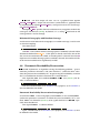
Input syntax We give below this model using the IMITATOR syntax. Note that
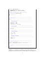
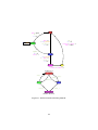
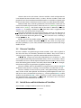
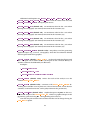
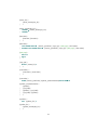
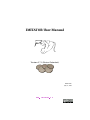
this model is given in graphical form in Fig. 2.1.1
1
2
3
4
5
6
7
8
9
10
11
12
13
14
15
16
(* ***********************************************************
IMITATOR MODEL
*
*
* Fischer ’ s mutual exclusion protocol
*
: Fischer ’ s mutual exclusion protocol with 2 processes
* Description
: Not 2 processes together in the c r i t i c a l section
* Correctness
( location obs_violation unreachable )
: PAT l i b r a r y of benchmarks
* Source
: ?
* Author
Input
by
: Etienne Andre
*
*
: 2012/10/08
* Created
: 2015/07/20
* Last modified
*
* IMITATOR version : 2.7 − beta4
*********************************************************** *)
17
18
19
20
21
var
x1 , ( * proc1 ’ s clock * )
x2 , ( * proc2 ’ s clock * )
: clock ;
22
23
24
25
turn ,
counter
: discrete ;
26
27
28
29
delta ,
gamma
: parameter ;
30
31
32
IDLE = −1
: constant ;
33
34
35
36
37
(* ********************************************************** *)
automaton proc1
(* ********************************************************** *)
synclabs : access_1 , enter_1 , exit_1 , no_access_1 , try_1 , update_1 ;
38
39
40
loc i d l e 1 : while True wait { }
when turn = IDLE sync tr y_1 do { x1 ’ = 0} goto a c t i v e 1 ;
41
42
43
loc a c t i v e 1 : while x1 <= d e l t a wait { }
when True sync update_1 do { turn ’ = 1 , x1 ’ = 0} goto check1 ;
44
45
46
loc check1 : while True wait { }
when x1 >= gamma & turn = 1 sync access_1 do { x1 ’ = 0} goto access1 ;
1 This LAT X representation, that makes use of the LAT X TikZ library, was automatically output
E
E
by IMITATOR, using option -PTA2TikZ, followed by some manual positioning optimization.
6
47
48
49
( * No "<>" operator : hence we use both ’ > ’ and ’ < ’ * )
when x1 >= gamma & turn < 1 sync no_access_1 do { x1 ’ = 0}
when x1 >= gamma & turn > 1 sync no_access_1 do { x1 ’ = 0}
goto i d l e 1 ;
goto i d l e 1 ;
50
51
52
loc access1 : while True wait { }
when True sync enter_1 do { counter ’ = counter + 1} goto CS1 ;
53
54
55
loc CS1 : while True wait { }
when True sync e x i t _ 1 do { counter ’ = counter − 1 , turn ’ = IDLE , x1 ’ =
0} goto i d l e 1 ;
56
57
end ( * proc1 * )
58
59
60
61
62
63
(* ********************************************************** *)
automaton proc2
(* ********************************************************** *)
synclabs : access_2 , enter_2 , exit_2 , no_access_2 , try_2 , update_2 ;
64
65
66
loc i d l e 2 : while True wait { }
when turn = IDLE sync tr y_2 do { x2 ’ = 0} goto a c t i v e 2 ;
67
68
69
loc a c t i v e 2 : while x2 <= d e l t a wait { }
when True sync update_2 do { turn ’ = 2 , x2 ’ = 0} goto check2 ;
70
71
72
73
74
75
loc check2 : while True wait { }
when x2 >= gamma & turn = 2 sync access_2 do { x2 ’ = 0} goto access2 ;
( * No "<>" operator : hence we use both ’ > ’ and ’ < ’ * )
when x2 >= gamma & turn < 2 sync no_access_2 do { x2 ’ = 0} goto i d l e 2 ;
when x2 >= gamma & turn > 2 sync no_access_2 do { x2 ’ = 0} goto i d l e 2 ;
76
77
78
loc access2 : while True wait { }
when True sync enter_2 do { counter ’ = counter + 1} goto CS2 ;
79
80
81
loc CS2 : while True wait { }
when True sync e x i t _ 2 do { counter ’ = counter − 1 , turn ’ = IDLE , x2 ’ =
0} goto i d l e 2 ;
82
83
end ( * proc2 * )
84
85
86
87
88
89
(* ********************************************************** *)
automaton observer
(* ********************************************************** *)
synclabs : enter_1 , enter_2 , exit_1 , e x i t _ 2 ;
90
91
92
93
loc obs_waiting : while True wait { }
when True sync enter_1 goto obs_1 ;
when True sync enter_2 goto obs_2 ;
94
95
96
97
loc obs_1 : while True wait { }
when True sync e x i t _ 1 goto obs_waiting ;
when True sync enter_2 goto obs_violation ;
98
7
99
100
101
loc obs_2 : while True wait { }
when True sync e x i t _ 2 goto obs_waiting ;
when True sync enter_1 goto obs_violation ;
102
103
104
( * NOTE: no outgoing action to reduce s t a t e space * )
loc obs_violation : while True wait { }
105
106
end ( * observer * )
107
108
109
110
111
112
113
114
(* ********************************************************** *)
(* I n i t i a l state *)
(* ********************************************************** *)
init :=
( *−−−−−−−−−−−−−−−−−−−−−−−−−−−−−−−−−−−−−−−−−−−−−−−−−−−−−−−−−−−−
INITIAL LOCATION
−−−−−−−−−−−−−−−−−−−−−−−−−−−−−−−−−−−−−−−−−−−−−−−−−−−−−−−−−−−−* )
115
& loc [ proc1 ] = i d l e 1
& loc [ proc2 ] = i d l e 2
& loc [ observer ] = obs_waiting
116
117
118
119
( *−−−−−−−−−−−−−−−−−−−−−−−−−−−−−−−−−−−−−−−−−−−−−−−−−−−−−−−−−−−−
INITIAL CLOCKS
120
121
−−−−−−−−−−−−−−−−−−−−−−−−−−−−−−−−−−−−−−−−−−−−−−−−−−−−−−−−−−−−* )
122
& x1 >= 0
& x2 >= 0
123
124
125
( *−−−−−−−−−−−−−−−−−−−−−−−−−−−−−−−−−−−−−−−−−−−−−−−−−−−−−−−−−−−−
INITIAL DISCRETE
126
127
−−−−−−−−−−−−−−−−−−−−−−−−−−−−−−−−−−−−−−−−−−−−−−−−−−−−−−−−−−−−* )
128
& turn = IDLE
& counter = 0
129
130
131
( *−−−−−−−−−−−−−−−−−−−−−−−−−−−−−−−−−−−−−−−−−−−−−−−−−−−−−−−−−−−−
PARAMETER CONSTRAINTS
132
133
−−−−−−−−−−−−−−−−−−−−−−−−−−−−−−−−−−−−−−−−−−−−−−−−−−−−−−−−−−−−* )
134
& d e l t a >= 0
& gamma >= 0
135
136
137
;
138
139
140
141
142
(* ********************************************************** *)
( * Property s p e c i f i c a t i o n * )
(* ********************************************************** *)
property : = unreachable loc [ observer ] = obs_violation ;
143
144
145
146
147
(* ********************************************************** *)
( * The end * )
(* ********************************************************** *)
end
Header Let us comment this case model by starting with the header. First, text
in comments gives generalities about the model (author, date, description, etc.).
8
The form is not normalized, but it could be in the future, so it is strongly advised
to follow this form.2
Variable declarations The variable declarations starts with keyword var.
This model contains two clocks: x1 is process 1’s clock, and x2 is process 2’s
clock.
This model contains two parameters: delta is the parametric duration specifying how long a process is idle at most, whereas gamma is the parametric duration specifying the minimum duration between the time a process checks for the
availability of the critical section and the time the same process indeed enters
the critical section (if it is still available).
Two discrete variables (i.e., global, integer-valued variables, see Section 3.2)
are used: turn checks which process is attempting to enter the critical section;
counter records how many processes are in the critical section (this variable
will not be used for the verification, but was used in the original PAT model, and
we choose to keep it).
Finally, a global constant IDLE is set to -1 (just as in the original PAT model),
and encodes that no process is attempting to enter the critical section.
Automata This model contains three IPTA: the first and second ones (proc1
and proc2) model the first and second process, respectively. The third one
(observer) is an observer, i.e., an IPTA that checks the system behavior without modifying it.
The first process Let us first describe the IPTA proc1 (a graphical representation is given in Fig. 2.1a). This IPTA uses six actions, given in the synclabs
declaration.
proc1 is initially in location idle1, with no invariant (depicted by while
True wait {}). At any time, when the discrete variable turn is equal to IDLE,
then this IPTA may synchronize on action try_1, reset its clock x1, and enter
location active1.
The invariant of this location is x1 <= delta, i.e., proc1 can only remain
in active1 as long as the value of x1 does not exceed delta. At any time, this
IPTA may synchronize on action update_1, reset its clock x1 and set the global
variable turn to 1, and enter location check1.
In location check1, the process wait at least gamma time units (modeled by
the inequality x1 >= gamma, in all outgoing transitions). If turn is still equal
to 1 (that is, no other process attempted in the meanwhile to enter the critical
section), then process 1 is indeed ready to enter the critical section, by synchronizing access_1 and resetting x1. If turn is different from 1 (that is, another
2 An empty model template with all these comments ready to be filled out (containing also a
sample IPTA and its initial definitions) is available at:
https://github.com/etienneandre/imitator/blob/master/examples/model.imi.
9
idle1
turn = IDLE
try_1
x1 := 0
x1 6 delta
turn 6= 1
∧ x1 > gamma
active1
exit_1
x1 := 0
counter := counter − 1
turn := IDLE
no_access_1
x1 := 0
update_1
x1 := 0
turn := 1
check1
∧
x1 > gamma
turn = 1
access_1
x1 := 0
access1
CS1
enter_1
counter := counter + 1
(a) Process 1
obs_waiting
exit_1
enter_2
exit_2
enter_1
obs_1
obs_2
enter_2
enter_1
obs_violation
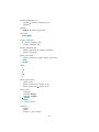
(b) PTA observer
Figure 2.1: Fischer mutual exclusion protocol
10
process attempted in the meanwhile to enter the critical section, and it is not
safe for process 1 to enter), then process 1 returns to its idle location, by synchronizing no_access_1 and resetting x1. Note that we have to use two transitions
checking that either turn < 1 or turn > 1 to compensate that the “different
from” operator (“6=”) is not (yet) supported by IMITATOR.
In location access1, process 1 can remain any time, and eventually enters
the critical section by synchronizing enter_1 and incrementing the global variable counter by 1.
In location CS1, process 1 can remain any time, and eventually leaves it, by
decrementing the global variable counter by 1, and setting the global variable
turn to its initial value IDLE.
The second process Process 2 is identical to process 1, except that x1 is replaced with x2, and that the value of turn becomes 2.
The observer The observer is in charge to check that no more than one process
is in critical section at the same time.3 This observer will detect that this situation happens if an action enter_1 is followed by an action enter_2 without an
action exit_1 in between (or symmetrically if an action enter_2 is followed by
an action enter_1 without an action exit_2 in between). Note that the observer simply observes the system state, and synchronizes on the actions used
by proc1 and proc2; it does not use any clock nor variable.
A graphical representation of the IPTA observer is given in Fig. 2.1b.
Initial definitions The initial state is defined the part of the file following
init :=. This part must contain the initial location of each IPTA. For example,
loc[proc1] = idle1 states that proc1 is initially in location idle1.
The initial definition may (only may, see Section 3.3) give an initial value to
the clocks, for example requiring them to be equal to some constant (typically 0).
Here, clocks are only bound to be greater or equal to 0.
The initial definition should assign a constant value to each discrete variable: here turn is initially equal to IDLE, and counter is initially equal to 0.
Finally, parameters are bound to be positive or null (this is not assumed by
default by IMITATOR, so users are strongly advised to add this constraint).
Note that the initial definition can introduce more complex constraints on
clocks, parameters and discrete variables; see Section 3.3 for details.
3 This observer is not really necessary to check the correctness of this protocol; instead
of adding this observer and checking unreachable loc[observer] = obs_violation, one
could just check either counter > 1 or loc[proc1] = CS1 & loc[proc2] = CS2. However,
IMITATOR does not (yet) support checking global variables or more that one location in the
unreachable property (which should be fixed very soon!); furthermore, introducing an observer
is also useful, as it is often used for verification.
11
Property specification In this model, the correctness property is that two processes cannot be in the critical section at the same time; as explained above, this
is equivalent to the fact that the obs_violation location of the observer IPTA
is unreachable. This is input in the model as follows:
property := unreachable loc[observer] = obs_violation;
More elaborate properties are detailed in Section 4.3 (however, they all reduce to
reachability, so more complex properties such as Büchi-like properties or fairness are not yet supported by IMITATOR).
Parameter synthesis Finally, let us run IMITATOR on this case study. Quite
naturally, what we would be interested in is knowing for which parameter valuations this protocol is correct, i.e., no more than one process can be present in the
critical section at one time. Assuming this model is input in file fischer.imi,
the command calling IMITATOR is as follows:
$ ./imitator fischer.imi -mode EF -merge
In this command, -mode EF calls the algorithm EFsynth that synthesizes
valuations reaching a given location (see Section 4.2); and -merge is a merging technique reducing the state space that, for this model, ensures termination
(see [AFS13] for more details on merging).
The result of the call to IMITATOR is
Final constraint such that the property is *violated* (1
constraint):
delta >= gamma
& gamma >= 0
That is, the system is safe if delta < gamma, which is the well-known constraint ensuring mutual exclusion for this protocol.
12
Chapter 3
IMITATOR Parametric Timed
Automata
3.1 Formal Definition
IMITATOR performs parametric verification of models specified using networks
of IMITATOR parametric timed automata (hereafter NIPTA).
An IMITATOR parametric timed automaton (hereafter IPTA) is a variant of
parametric automata (as introduced in [AHV93]). A first difference between
IPTA and the PTA of [AHV93] is that IPTA have no accepting / final location; furthermore, IPTA augment the expressiveness of PTA with several features such as
invariants, discrete (integer) variables, complex guards and invariants (i.e., not
only comparing a single clock to a single parameter), stopwatches (i.e., the ability to stop some clocks in some locations), and arbitrary clock updates (i.e., not
necessarily to 0).
3.1.1 Linear Constraints
Clocks, Parameters, Discrete Variables Clocks are real-valued variables all
evolving at the same rate (unless they are stopped, which is allowed in
IMITATOR). A set of clocks is X = {x1 , . . . , xH }; a clock valuation is w : X → R>0 .
Parameters are rational-valued variables, that act as unknown constants. A
set of parameters is P = {p1 , . . . , pM }; a parameter valuation is a function v : P →
R. We will often identify a valuation v with the point (v(p1 ), . . . , v(pM )).
Discrete variables are integer-valued variables. A set of discrete variables is
D = {d1 , . . . , dJ }; a discrete variable valuation is a function δ : D → N.
Linear Constraints Let us formalize the set of linear constraints allowed in
IMITATOR. Given a set of variables Var = {z1 , . . . , zN } (in the following, this set
will be instantiated with X and/or P and/or D), a linear term over Var is an ex-
13
pression of the form
X
αi zi + d
16i6n
for some n ∈ N, where zi ∈ Var, αi ∈ Q, for 1 6 i 6 n, and d ∈ Q.
An atomic constraint over Var is an expression of the form lt ≺ 0 where lt is
a linear term over Var, and ≺∈ {, 6, >, }.
A constraint over Var is a conjunction of atomic constraints. We denote by
LT (Var ) the set of linear terms over Var, and by L C (Var ) the set of constraints
over Var. In IMITATOR, we will consider constraints belonging to sets such as
L C (X ∪ P) (i.e., the set of constraints over clocks and parameters), or L C (X ∪
P∪D) (i.e., the set of constraints over clocks, parameters and discrete variables).
3.1.2
IMITATOR Parametric Timed Automata
We can now give a formal definition of IPTA.
Let denote the unobservable action.
Definition 1 (IPTA). An IMITATOR parametric timed automaton ( IPTA) is a tuple A = hΣ, L, linit , D, X, P, I, S, →i, where:
• Σ is a finite set of actions;
• L is a finite set of locations;
• linit ∈ L is the initial location;
• D is a set of integer-valued variables;
• X is a set of clocks;
• P is a set of parameters;
• I : L → L C (X ∪ P ∪ D) assigns to every location l a constraint over all
variables, called the invariant of l;
• S : L → X assigns to a every location a list of clocks that are stopped in this
location;
• → is a set of edges (l, g, a, Xup , Dup , l 0 ), where l, l 0 ∈ L are the source and
destination locations, g ∈ L C (X ∪ P ∪ D) is a constraint over all variables
(called guard of the transition), a ∈ Σ ∪ {} is the action associated with the
transition, Xup : X → LT (X ∪ P ∪ D) is the update function for clocks, and
Dup : D → LT (D) is the update function for discrete variables.
In the following, we explain this definition.
14
Guards and invariants Guards and invariants in IMITATOR are linear constraints over all variables. For example, the following expression can be used
in a guard or an invariant:
i1 + .5 x1 + 3 x2 >= 2 p1 - i2 & p2 < 1/3
where i1, i2 are discrete variables, x1, x2 are clocks and p1, p2 are parameters.
This syntax includes in particular diagonal constraints (e.g., x1 - x2 <= 2), not
always supported in other model-checking tools.
Actions Transitions can be synchronized on an action in Σ, or have no synchronized action (“”), which is often referred to in the literature as a silent
transition, or an -transition. For the semantics of the synchronization model
between various IPTA, refer to Section 3.4.
Clock updates Observe that clocks can be updated to any value, i.e., a clock
can be assigned not only to 0, but to any linear term over the other clocks, the
parameters and the discrete variables. However, discrete variables can only be
assigned to a linear term over D (including a constant). If clocks are always reset
(i.e., not assigned to more complex linear terms), IMITATOR will apply some
optimizations that (may) increase the analysis speed.
Stopwatches There are no distinction between clocks and stopwatches. That
is, any clock can potentially be stopped in some location. IMITATOR will detect whether a model has or not stopwatches; if there is no stopwatch in some
model, IMITATOR will apply some optimizations that (may) increase the analysis speed.
3.1.3 Networks of
IMITATOR Parametric Timed Automata
Definition
2
(NIPTA).
Given
a
set
of
IPTA
Ai
=
hΣi , Li , (linit )i , Di , Xi , Pi , Ii , Si , →i i, 1 6 i 6 N for some N ∈ N, a network
of IPTA ( NIPTA) is a tuple hΣ, D, X, P, {Ai | 1 6 i 6 N}, Cinit i, where:
• Σ=
S
• D=
S
• X=
S
16i6N Xi
is the set of all clocks;
• P=
S
16i6N Pi
is the set of all parameters;
16i6N Σi
is the set of all actions;
16i6N Di
is the set of all discrete variables;
• Cinit ∈ L C (X ∪ P ∪ D) is the initial constraint over D, X and P.
15
Observe that each set of actions, discrete variables, clocks and parameters
is not disjoint between all IPTA. That is, actions, discrete variables, clocks and
parameters may be shared between different IPTA. If a variable is required to be
local to an IPTA, then it should just not be used in any other IPTA of the model.
Different from many tools for (parametric) timed automata, clocks are not
necessarily initially equal to 0 (this is similar to H Y T ECH [HHWT95] but different
from U PPAAL [LPY97]). The initial value of the clocks is defined by Cinit (see
Section 3.3). If nothing is defined in Cinit , then their value is supposed to be
arbitrary (any real value greater or equal to 0).
Note that parameters are not assumed positive; however, the behavior of
IMITATOR has not been tested for negative parameters, and it is strongly advised to constrain them to be positive in Cinit (if it is not the case, a warning is
issued by IMITATOR).
Finally, note that the number of IPTA, locations, variables and actions that
can be defined in a model is bounded in IMITATOR by some very large number (most probably 232 ); but, well, you don’t seriously plan to build such a large
model, do you?
3.2 Discrete Variables
Discrete variables1 are global integer-valued variables. Their value is global, in
the sense that they are shared by all IPTA of the model. They can be seen as
syntactic sugar to represent a possibly unbounded number of locations.
In IMITATOR, integers are exact and unbounded, just as in maths (i.e.,, they
are not represented using a limited number of bits, such as 32 or 64 bits). Hence,
no overflow can occur, and the representation of the constraints is always exact.
Note that floating-point numbers are totally absent from the IMITATOR implementation (except for th generation of graphical outputs).
Discrete variables must be initialized to a single constant value in the init
definition; if they are not, a warning is issued, and they are arbitrarily set to 0.
Discrete variables can be tested in guards, and updated along transitions.
They are first tested, then updated. If two IPTA in parallel update the same variable on the same synchronized transition (e.g., an IPTA performs i' = 2 while
another one performs i' = 3), then a warning is issued, and the behavior of
the NIPTA becomes unspecified (i.e., IMITATOR will choose one or the other
assignment in a non-deterministic manner).
3.3 Initial State and Initialization of Variables
For each IPTA, a unique initial location must be defined.
1 The name “discrete variable” comes from H Y T ECH .
16
For variables, the definition of the initial value is very permissive in
IMITATOR. Clocks are not necessarily equal to 0, and parameters are not even
necessarily positive.
Parameters and clocks can be initially bound by any linear constraint over
parameters, clocks, and discrete variables. That is, we can define initial constraints such as:
x1 + x2 <= 2 p1 + 0.5 p2 - i.
However, discrete variables must be initialized to a constant integer. Given
a discrete variable i, if the definition of the initial state does not contain an
equality of the form i = ... followed by a linear term in LT (X ∪ P ∪ D), then
IMITATOR will assume that i is initially set to 0, and will issue a warning.
3.4 Synchronization Model
By default, all IPTA of an IMITATOR model declare their set of actions.2
The IMITATOR synchronization model is such that all IPTA declaring an
action must synchronize together on this action. This can be seen as a strong
broadcast. That is, for a transition labeled with action a to be executed, all IPTA
declaring a must be ready to execute a locally. Otherwise, this transition cannot
be taken (yet).
If an IPTA declares an action a that is never used in this IPTA, then action a
will never be executed in the entire model.3
3.5 Constants
IMITATOR supports global constants, i.e., a variable the value of which is known
once for all. The syntax is the following one:
c = 1:
constant;
Then, any occurrence of c in the model is replaced with 1.
Constants are (unbounded, exact) integers.
Hint 1. In fact, a variable (e.g., a parameter) can be turned to a constant as follows
in the definition of the parameters:
p = 2:
2 An
alternative
is
an
automatic
parameter;
recognition
-sync-auto-detect in Chapter 7.
of
the
actions
used,
see
option
IMITATOR will detect this situation and will entirely delete this action from the
model, while issuing a warning.
3 In this case,
17
This is equivalent to replacing p with 2 everywhere in the model; this is particularly useful when some parameters should be instantiated. In contrast, if the
parameter is instantiated in the initial definition, IMITATOR still counts it as a
parameter, which makes all constraints suffer from an additional dimension.
18
Chapter 4
Parameter Synthesis Using
IMITATOR
We give here the commands corresponding to the main analysis features of
IMITATOR. We only give the most useful options. For more detailed commands,
and a complete list of options, see Chapter 7.
4.1 State Space Computation
IMITATOR
can compute the entire symbolic state space (“parametric zone
graph”). Of course, the state space may be infinite, and this analysis is not guaranteed to terminate.
The standard command is:
$ ./imitator model.imi -mode statespace -output-states
The option -output-states generates a file with a textual description of all
states (without this option, IMITATOR will not output anything).
IMITATOR can also output the trace set in a graphical form using option
-output-trace-set.
4.2 EF-Synthesis
A main problem in parametric timed automata is to compute the set of parameter valuations for which some location (for instance, an error location) is reachable.
The property must be specified as follows, at the end of the model (after the
initial state definition):
property := unreachable loc[AUTOMATON] = LOCATION
where AUTOMATON is an automaton name, and LOCATION is a location name.
19
The algorithm EFsynth implemented in IMITATOR is a basic breadth-first
procedure, close to the one described in [AHV93, JLR15]. Of course, the EFemptiness problem being undecidable [AHV93], the analysis is not guaranteed
to terminate.
The standard command is:
$ ./imitator model.imi -mode EFsynth -merge -incl
The options -merge and -incl are optional, but generally greatly
increase the analysis efficiency and the termination.
The option
-dynamic-elimination can also be used to reduce the state space.
IMITATOR can also output the trace set in a graphical form (option
-output-trace-set), output the constraint synthesized in a graphical form in
two dimensions (option -output-cart), or output the result to a text file (option -output-result).
4.3 Parametric Verification using Properties
IMITATOR basically only supports bad state reachability synthesis on the one
hand, and algorithms such as the inverse method and the cartography on the
other hand. However, many correctness properties can be encoded using reachability using observers (see [ABL98, ABBL98, And13b]).
Encoding observers can be done manually (using ad-hoc IPTA), or using predefined correctness properties commonly met in the literature.
If using a predefined property, the property must be specified as follows, at
the end of the model (after the initial state definition):
property := [PROP]
[PROP] must conform to one of the following patterns, where AUTOMATON is
an automaton name, LOCATION is a location name, a, a1, a2 are actions, and the
deadline d is a (possibly parametric) linear expression:
• property := unreachable loc[AUTOMATON] = LOCATION
• property := if a2 then a1 has happened before
• property := everytime a2 then a1 has happened before
• property := everytime a2 then a1 has happened once before
• property := a within d
• property := if a2 then a1 has happened within d before
• property := everytime a2 then a1 has happened within d
before
• property := everytime a2 then a1 has happened once within
d before
20
• property := if a1 then eventually a2 within d
• property := everytime a1 then eventually a2 within d
• property := if a1 then eventually a2 within d once before
next
• property := sequence a1, ..., an
• property := always sequence a1, ..., an
The semantics of these properties is detailed in [And13b].
Then, the command to synthesize parameters is the same as for the EFsynthesis:
$ ./imitator model.imi -mode EFsynth -merge -incl
4.4 Inverse Method: Trace Preservation
Given a NIPTA and a reference parameter valuation, the inverse method IM
synthesizes a parameter constraint such that, for any parameter valuation
in that constraint, the set of traces is the same as for the reference valuation [ACEF09]. This problem is known as the trace preservation synthesis. The
trace-preservation emptiness problem being undecidable [AM15], the analysis
is not guaranteed to terminate (although it often does in practice).
The command is:
$ ./imitator model.imi model.pi0
The reference valuation is described in model.pi0.
IMITATOR can also output the trace set in a graphical form (option -output-trace-set), or output the result to a text file (option
-output-result).
4.5 Behavioral Cartography
Given a NIPTA and a bounded parameter domain, the behavioral cartography BC synthesizes tiles, i.e., parameter domains such that for any parameter
valuation in that domain, the set of traces is the same [AF10]. The corresponding
problem being undecidable, the analysis is not guaranteed to terminate; when
it terminates, it may also leave “holes”, i.e., parameter domains not covered by
any tile.
The command is:
$ ./imitator model.imi model.v0 -mode cover
The bounded parameter domain is described in model.v0.
21
IMITATOR
can also output all trace sets in a graphical form (option
-output-trace-set), output the constraints synthesized in a graphical form
in two dimensions (option -output-cart), or output the result to a text file (option -output-result).
The option -step specifies the interval between any two points of which the
coverage is checked (see [AF10]). By default, it is 1; setting
coverage when 1 was not enough.
1
3
often leads to full
Behavioral Cartography with Random Coverage
An alternative to the behavioral cartography is a random coverage; it can be seen
as a kind of sampling.
The command is:
$ ./imitator model.imi model.v0 -mode randomXX
where XX is the number of times an integer point is randomly selected within
the domain defined in model.v0. If this point is already covered by one of the
tiles, the inverse method is not called, an another point is selected. Note that XX
represents the number of integer points randomly selected; the number of calls
to the inverse method can be significantly smaller.
4.6 Parametric Reachability Preservation
IMITATOR implements an algorithm solving the following problem:
“given a
reference parameter valuation v and some location l, synthesize other valuations that preserve the reachability of l”. By preserving the reachability, we mean
that l is reachable for the other valuations iff l is reachable for v.
This algorithm PRP, that combines EFsynth and IM (see [ALNS15] for details), is called as follows:
$ ./imitator model.imi model.pi0 -PRP
Note that a bad location (as in Section 4.2) or a property (as in Section 4.3)
must be defined in the model.
Parametric Reachability Preservation Cartography
An extension of PRP to the cartography (named PRPC) is also available: PRPC
synthesizes parameter constraints in which the (non-)reachability of l is uniform. PRPC was showed in [ALNS15] to be a good alternative to EFsynth, especially when distributed.
This algorithm PRPC is called as follows:
$ ./imitator model.imi model.v0 -mode cover -PRP
Again, a bad location (as in Section 4.2) or a property (as in Section 4.3) must
be defined in the model.
22
Chapter 5
Graphical Output and Translation
Again, we only give the most useful options. For more detailed commands, and
a complete list of options, see Chapter 7.
5.1 Trace Set
To generate the trace set of a given computation in a graphical form, use:
$ ./imitator model.imi [options] -output-trace-set
IMITATOR will generate a file model.jpg.
Note that, beyond about 1,000
states or 1,000 transitions, the dot utility (responsible to generate the trace set)
may crash.
Using -output-trace-set-nodetails makes a more compact representation (but is also less informative).
5.2 Constraints and Cartography
To generate the constraint generated by IMITATOR in a 2-dimensional plot (using the plot utility), use:
$ ./imitator model.imi [options] -output-cart
will generate file model_cart_ef.png if the algorithm is
model_cart_bc.png if the algorithm is BC and its variant, or
model_cart_patator.png if the algorithm is the distributed BC and its
This
EFsynth,
variants.
The 2 dimensions chosen for the plot are the first two (non-constant) parameter dimension in the model.
Additional useful options are -output-cart-x-min, -output-cart-x-max,
-output-cart-y-min, -output-cart-y-max to tune the values of the axes, and
-output-graphics-source to keep the plot source.
The graphical output of the constraint is not yet available for the inverse
method.
23
5.3 Export to JPEG
To generate a graphic representation of the model without performing any analysis, use:
$ ./imitator model.imi -PTA2JPG
IMITATOR will generate a file model-pta.jpg.
5.4 Export to LATEX
To generate a LATEX representation of the model (using the tikz package) without performing any analysis, use:
$ ./imitator model.imi -PTA2TikZ
IMITATOR will generate a file model.tex. This file is a standalone LATEX file
containing a single figure, which contains the different IPTA in subfigure environments. The node positioning is not yet supported (locations are depicted
vertically), so you may need to manually position all nodes, and bend some transitions if needed.
24
Chapter 6
Inside the Box
6.1 Language and Libraries
In short,
code.
IMITATOR is written in OCaml, and contains about 26,000 lines of
IMITATOR makes use of the following external libraries:
• The OCaml ExtLib library (Extended Standard Library for Objective Caml);
• The GNU Multiple Precision Arithmetic Library (GMP);
• The Parma Polyhedra Library (PPL) [BHZ08], used to compute operations
on polyhedra.
6.2 Symbolic States
Verification of timed systems (and specially parametric timed systems) is necessarily done in a symbolic manner, in the sense that the timing information is
abstracted by clock constraints. However, IMITATOR does not perform what is
referred to as symbolic model checking; in other words, the representation of locations in IMITATOR is explicit (and not symbolic using, e.g., binary decision
diagrams).
In short, a symbolic state in IMITATOR is made of the following elements:
• the current location (index) of each IPTA;
• the current value of the (integer-valued) discrete variables;
• a constraint on X ∪ P ∪ D representing the continuous information.
In IMITATOR, all integers (i.e., the value of the discrete variables and the coefficients used in the constraints) are unbounded integers (implemented using
GMP).
25
6.3 Installation
This document does not aim at explaining how to install IMITATOR. See the
installation information available on the website for the most up-to-date information.
Binaries and source code packages are available on IMITATOR’s Web
page [IMI15]. Several standalone binaries are provided for Linux systems, that
require no installation.
26
Chapter 7
List of Options
The options available for IMITATOR are explained in the following.
Note that some more options are available in the current implementation
of IMITATOR. If these options are not listed here, they are experimental (or
deprecated). If needed, more information can be obtained by contacting the
IMITATOR team.
-acyclic (default: false) Does not test if a new state was already encountered.
Without this option, when IMITATOR encounters a new state, it checks if it has
been encountered before. This test may be time consuming for systems with a
high number of reachable states. For acyclic systems, all traces pass only once
by a given location. As a consequence, there are no cycles, so there should be
no need to check if a given state has been encountered before. This is the main
purpose of this option.
However, be aware that, even for acyclic systems, several (different) traces
can pass by the same state. In such a case, if the -acyclic option is activated,
IMITATOR will compute twice the states after the state common to the two
traces. As a consequence, it is all but sure that activating this option will lead
to an increase of speed.
Note also that activating this option for non-acyclic systems may lead to an
infinite loop in IMITATOR.
-check-ippta (default: false) Check that every new symbolic state contains
an integer point (i.e., a point in the X ∪ P dimension). If not, raises an exception.
-check-point (default: false) In the inverse method, checks at each iteration
whether the accumulated parameter constraint is restricted to the reference parameter valuation. Note that this option is not implemented as nicely as it could
be, and can hence turn very costly.
27
-completeIM (default: false) Returns a complete result for the inverse method
for deterministic PTA, i.e., returns a conjunction of negations of convex parameter constraints. The result may result in a large list of such constraints, and may
hence be complicated to interpret.
-contributors Print the list of contributors and exits.
-depth-limit <limit> (default: none) Limits the depth of the exploration
of the state space. In the cartography mode, this option gives a limit to each call
to the inverse method. Setting -depth-limit guarantees the termination of any
execution of IMITATOR, but not necessarily the correctness of the algorithms.
-distributed <mode> (default: not distributed) Distributed version of the
behavioral cartography. Various distribution modes are possible:
no Non-distributed mode (default)
static Static domain decomposition [ACN15]
sequential Master-worker scheme with sequential point distribution [ACE14]
randomXX Master-worker scheme with random point distribution (e.g.,
random5 or random10); after XX successive unsuccessful attempts (where
the generated point is already covered), the algorithm will switch to an
exhaustive sequential iteration [ACE14]
shuffle Master-worker scheme with shuffle point distribution [ACN15]
dynamic Master-worker dynamic subdomain decomposition [ACN15]
-dynamic-elimination (default: false) Dynamic elimination of clocks that
are known to not used in the future of the current state [And13a].
-fromGrML (default: false) Does not use the standard input syntax described
here, but a GrML input syntax. This is used when interfacing IMITATOR with the
CosyVerif platform [AHHH+ 13]. Note that, in that case, not all syntactic features
of IMITATOR are supported.
-IMK (default: false) Uses a variant of the inverse method that returns a constraint such that no π0 -compatible state is reached; it does not guarantee however that any “good” state will be reached (see [AS13]).
-IMunion (default: false) Uses a variant of the inverse method that returns the
union of the constraints associated to the last state of each path (see [AS13]).
28
-incl (default: false) Consider an inclusion of region instead of the equality when performing the Post operation. In other terms, when encountering a
new state, IMITATOR checks if the same state (same location and same constraint) has been encountered before and, if so, discards this “new” state. However, when the -incl option is activated, it suffices that a previous state with
the same location and a constraint greater than or equal to the constraint of the
new state has been encountered to stop the analysis. This option corresponds
to the way that, e.g., H Y T ECH works, and suffices when one wants to check the
non-reachability of a given bad state.
-merge (default: false) Use the merging technique of [AFS13]. This option is
safe (and advised) for the EFsynth algorithm.
However, not all the properties of the inverse method are preserved when
using merging (see [AFS13] for details).
-mode (default: inversemethod) The mode for IMITATOR.
statespace
Generation of the entire parametric state space
(see Section 4.1)
EF
Parametric non-reachability analysis (EFsynth [JLR15])
(see Section 4.2)
inversemethod Inverse method
(see Section 4.4)
cover
Behavioral Cartography Algorithm with full coverage
(see Section 4.5)
randomXX
Behavioral Cartography Algorithm with XX iterations
(see Section 4.5)
-no-random (default: false) In the inverse method, no random selection of the
π0 -incompatible inequality (select the first found). By default, select an inequality in a random manner.
-output-cart (default: off ) After execution of the behavioral cartography
or EFsynth, plots the generated zones as a .png file. This will generate file
model_cart_ef.png if the algorithm is EFsynth, model_cart_bc.png if the algorithm is BC and its variant, or model_cart_patator.png if the algorithm is
the distributed BC and its variants. If the model contains more than two parameters, then -output-cart will plot the projection of the generated zones on the
first two parameters of the model (or on the two varying parameters in the case
of BC).
This option makes use of the external utility graph, which is part of the GNU
plotting utils, available on most Linux platforms. The generated files will be located in the same directory as the source files, unless option -output-prefix
is used.
29
Additional useful options are -output-cart-x-min, -output-cart-x-max,
-output-cart-y-min, -output-cart-y-max to tune the values of the axes, and
-output-graphics-source to keep the plot source.
-output-cart-x-min (default: off ) Set minimum value for the x axis when
plotting the cartography (not entirely functional in all situations yet).
-output-cart-x-max (default: off ) Set maximum value for the x axis when
plotting the cartography (not entirely functional in all situations yet).
-output-cart-y-min (default: off ) Set minimum value for the y axis when
plotting the cartography (not entirely functional in all situations yet).
-output-cart-y-max (default: off ) Set maximum value for the y axis when
plotting the cartography (not entirely functional in all situations yet).
-output-graphics-source (default: false) Keep file(s) used for generating
graphical output (e.g., trace set, cartography); these files are otherwise deleted
after the generation of the graphics.
-output-prefix (default: <input_file>) Set the path prefix for all generated
files. The path can be either relative (to the path to the ./imitator binary) or
absolute, and must be followed by the file name.
Examples:
• -output-prefix log
• -output-prefix ./log
• -output-prefix /home/imitator/outputs
-output-result (default: false) Writes the result of the analysis to a file
named <input_file>.result.
-output-states (default: false) Generates a file <input_file>.states describing the reachable states in plain text (value of the location, of the discrete
variables, associated constraint, and its projection onto the parameters).
-output-trace-set (default: false) Graphical output using dot. In this case,
IMITATOR outputs a file <input_file>.jpg, which is a graphical output in the
jpg format, generated using dot, corresponding to the trace set.
Note that the path and the name of those two files can be changed using the
-log-prefix option.
30
-output-trace-set-nodetails (default: false) In the graphical output of
the trace set (see option -output-trace-set), does not provide detailed information on the local locations of the composed IPTA, and instead only outputs
the state id. Enabling this option may yield a smaller graph, which is useful when
generating large trace sets.
-output-trace-set-verbose (default: false) In the graphical output of the
trace set (see option -output-trace-set), provides very detailed information,
by adding to the right of the local locations of the composed IPTA the associated constraint as well. In addition, the parametric constraint is printed too.
Enabling this option will yield a very large graph, and it is useful (and readable)
mostly for very small trace sets.
-PRP (default: false) Option used to activate PRP or PRPC [ALNS15]. These
options must be used in addition to the -mode option. That is, in order to call
PRP, use:
$ ./imitator model.imi model.pi0 -PRP
And in order to call PRPC, use:
$ ./imitator model.imi model.v0 -mode cover -PRP
-PTA2GrML (default: false) Translates the input model to a GrML format (used
by CosyVerif [AHHH+ 13]), and exits.
-PTA2JPG (default: false) Translates the input model to a graphical, humanreadable form (in .jpg format), and exits.
-PTA2TikZ (default: false) Translates the input model to a LATEX representation
of the model (using the tikz package) without performing any analysis, and
exits. Note that node positioning is not (much) supported, so may want to edit
manually some positions.
-states-limit (default: none) Will try to stop after reaching this number of
states. Warning: the program may have to first finish computing the current iteration (i.e., the exploration of the state space at the current depth) before stopping.
-statistics (default: false) Print info on number of calls to PPL, and other
statistics about memory and time. Warning: enabling this option may slightly
slow down the analysis, and will certainly induce some extra computational time
at the end.
31
-step (default: 1) Step for the behavioral cartography. Integers can be used,
or rationals (in the form x/y).
IMITATOR considers that all the IPTA
declaring a given action must be able to synchronize all together, so that the
synchronization can happen. By default, IMITATOR considers that the actions
declared in an IPTA are those declared in the synclabs section. Therefore, if an
action is declared but never used in (at least) one IPTA, this label will never be
synchronized in the execution1 .
The option -sync-auto-detect allows to detect automatically the actions
in each IPTA: the actions declared in the synclabs section are ignored, and
IMITATOR considers as declared actions only the actions really used in this
IPTA.
-sync-auto-detect (default: false)
-time-limit <limit> (default: none) Try to limit the execution time (the
value <limit> is given in seconds). Note that, in the current version of
IMITATOR, the test of time limit is performed at the end of an iteration only
(i.e., at the end of the exploration of the state space at the current depth). In the
cartography mode, this option represents a global time limit, not a limit for each
call to the inverse method.
-timed (default: false) Add a timing information to each shell output of the
program.
-tree (default: false) Does not test if a new state was already encountered.
To be set only if the reachability graph is a tree with all states being different
(otherwise analysis may loop).
-verbose (default: standard) Give some debugging information, that may
also be useful to have more details on the way IMITATOR works. The admissible values for -verbose are given below:
mute
No output (the result can be output to a file using -output-result)
warnings Prints only warnings
standard Give little information (number of steps, computation time)
low
Give little additional information
medium Give quite a lot of information
high
Give much information
total
Give really too much information
-version Prints IMITATOR header including the version number and exits.
1 In such a case, action label is actually completely removed before the execution, in order to
optimize the execution, and the user is warned of this removal.
32
Chapter 8
Grammar
8.1 Variable Names
A variable name (represented by <name> in the grammar below) is a string starting with a letter (small or capital), and followed by a set of letters, digits and underscores (“_”). By letter we mean the 26 letters of the Latin alphabet, without
any diacritic mark.
The set of clock names, parameter names and discrete variable names must
(quite naturally) be disjoint. However, the sets of IPTA names, location names,
action names, and variable names are not required to be disjoint. That is, the
same name can be given to a clock, an automaton, an action and a location.
Furthermore, the names of the sets of locations of various IPTA are notnecessarily disjoint either: that is, a same name can be given to two different
locations in two different IPTA (and they still represent two different things).
8.2 Grammar of the Input File
The IMITATOR input model is described by the following grammar. Nonterminals appear hwithin angled parenthesesi. A non-terminal followed by two
colons is defined by the list of immediately following non-blank lines, each of
which represents a legal expansion. Input characters of terminals appear in
typewritter font. The meta symbol denotes the empty string.
The text in green is not taken into account by IMITATOR, but allows some
backward-compatibility with H Y T ECH files [HHWT95].
himitator_input i ::
hautomata_descriptionsi hinit i
We define each of those two components below.
33
8.2.1 Automata Descriptions
hautomata_descriptionsi ::
hdeclarationsi hautomatai
hdeclarationsi ::
var hvar_listsi
hvar_listsi ::
hvar_list i : hvar_typei ; hvar_listsi
| hvar_list i ::
<name>
| <name> = hrationali
| <name> , hvar_list i
| <name> = hrationali , hvar_list i
hvar_typei ::
clock
| discrete
| parameter
hautomatai ::
hautomatoni hautomatai
| hautomatoni ::
automaton <name> hprolog i hlocationsi end
hprolog i ::
hinitializationi hsync_labelsi
| hsync_labelsi hinitializationi
| hsync_labelsi
| hinitializationi
| hinitializationi ::
initially <name> hstate_initializationi ;
hstate_initializationi ::
& hconvex_predicatei
| hsync_labelsi ::
synclabs : hname_list i ;
34
hname_list i ::
hname_nonempty_list i
| hname_nonempty_list i ::
<name> , hname_nonempty_list i
| <name>
hlocationsi ::
hlocationi hlocationsi
| hlocationsi ::
loc <name> : while hconvex_predicatei hstop_opt i hwait_opt i htransitionsi
| urgent loc <name> : while hconvex_predicatei hstop_opt i hwait_opt i htransitionsi
hwait_opti ::
wait()
| wait
| hstop_opt i ::
stop{ hname_list i }
| htransitionsi ::
htransitioni htransitionsi
| htransitioni ::
when hconvex_predicatei hupdate_synchronizationi goto <name> ;
hupdate_synchronizationi ::
hupdatesi
| hsyn_labeli
| hupdatesi hsyn_labeli
| hsyn_labeli hupdatesi
| hupdatesi ::
do ( hupdate_list i )
hupdate_list i ::
hupdate_nonempty_list i
| 35
hupdate_nonempty_list i ::
hupdatei , hupdate_nonempty_list i
| hupdatei
hupdatei ::
<name> ' = hlinear_expressioni
hsyn_labeli ::
sync <name>
hconvex_predicatei ::
& hconvex_predicate_foli
| hconvex_predicate_foli
hconvex_predicate_foli ::
hlinear_constraint i & hconvex_predicatei
| hlinear_constraint i
hlinear_constraint i ::
hlinear_expressioni hrelopi hlinear_expressioni
| True
| False
hrelopi ::
<
| <=
| =
| >=
| >
hlinear_expressioni ::
hlinear_termi
| hlinear_expressioni + hlinear_termi
| hlinear_expressioni - hlinear_termi
hlinear_termi ::
hrationali
| hrationali <name>
| hrationali * <name>
| - <name>
| <name>
| ( hlinear_termi )
hrationali ::
hinteger i
hfloat i
| hinteger i / hpos_integer i
36
hinteger i ::
hpos_integer i
| - hpos_integer i
hpos_integer i ::
<int>
hfloat i ::
hpos_float i
| - hpos_float i
hpos_float i ::
<float>
8.2.2 Initial State
hinit i ::
hinit_declarationi hinit_definitioni hproperty_definitioni hprojection_definitioni hother_commandsi
hinit_declarationi ::
var init : region ;
| hother_commandsi ::
end hrest_of_commandsi
| hrest_of_commandsi ::
hanything i hrest_of_commandsi
| hanythingi ::
(
| )
| <name>
| init
| bad
hinit_definitioni ::
init := hregion_expressioni ;
hregion_expressioni ::
& hregion_expression_foli
| hregion_expression_foli
37
hregion_expression_foli ::
hstate_predicatei
| ( hregion_expression_foli )
| hregion_expression_foli & hregion_expression_foli
hstate_predicatei ::
loc [ <name> ] = <name>
| hlinear_constraint i
hloc_predicatei ::
loc[ <name> ] = <name>
hproperty_definitioni ::
property := hpatterni ;
| hpatterni ::
unreachable hloc_predicatei
| if <name> then <name> has happened before
| everytime <name> then <name> has happened before
| everytime <name> then <name> has happened once before
| if <name> then eventually <name>
| everytime <name> then eventually <name>
| everytime <name> then eventually <name> once before next
| <name> within hlinear_expressioni
| if <name> then <name> happened within hlinear_expressioni before
| everytime <name> then <name> happened within hlinear_expressioni before
| everytime <name> then <name> happened once within hlinear_expressioni before
| if <name> then eventually <name> within hlinear_expressioni
| everytime <name> then eventually <name> within hlinear_expressioni
| everytime <name> then eventually <name> within hlinear_expressioni once before next
| sequence hvar_list i
| sequence always hvar_list i
8.3 Grammar of the Reference Valuation File
The reference valuation file (usually named model.pi0) gives a constant value
to any parameter of the model; this file is used for IM and PRP.
It basically consists of a sequence of equalities parameter = constant separated (or not!) by the & symbol. All parameters of the model must be given a
valuation in this file; but the file may also use names that do not appear in the
model (a warning will just be issued).
Arithmetic expressions (using integers and rationals) can even be used instead of just constants.
38
8.4 Grammar of the Reference Hyperrectangle File
The hyperrectangle file (usually named model.v0) defines a bounded parameter domain, i.e., a hyperrectangle having as dimensions the parameters of the
model; this file is used for BC and PRPC.
It basically consists of a sequence of either equalities parameter =
constant or intervals parameter = constant .. constant separated (or
not!) by the & symbol. All parameters of the model must be given an interval
(possibly punctual) in this file; again, the file may also use names that do not
appear in the model (a warning will just be issued).
Again, arithmetic expressions (using integers and rationals) can even be
used instead of just constants.
8.5 Reserved Words
The following words are reserved keywords and cannot be used as names for
automata, variables, actions or locations.
always, and, automaton, bad, before, carto, clock, constant,
discrete, do, end, eventually, everytime, False, goto, happened, has,
if, init, initially, loc, locations, next, not, once, or, parameter,
projectresult, property, region, sequence, stop, sync, synclabs, then,
True, unreachable, urgent, var, wait, when, while, within
39
Chapter 9
Missing Features
Although we try to make IMITATOR as complete as possible, it misses some
features, not implemented due to lack of time (contributors are welcome!) or
due to complexity, or to keep the tool consistent. We enumerate in the following
what seems to us to be the “most missing” features and, when applicable, we
give hints to overcome these limitations.
9.1 ASAP Transitions
ASAP (as soon as possible) transitions are transitions that can be taken as soon
as all IPTA synchronizing with this transition can execute their local transition.
This is different from urgent transitions, that must be taken in 0 time. Here, time
can elapse, but not after all IPTA are ready to execute their local transition.
This is not supported by IMITATOR, and we do not see a way to simulate it
easily in the current implementation.
9.2 Parameterized Models
Parameterized models are understood here as models with an arbitrary number
of components (e.g., Fischer’s mutual exclusion protocol with n processes), that
would be instantiated (e.g., n = 15) before performing the analysis. IMITATOR
does not currently support such parameterized models, and one should use
copy/paste utilities to instantiate n models. For complicated models with
many processes, we usually write short scripts to generate the model (a script
CSMACDgenerator.py to model the varying part of parameterized models for
the CSMA/CD case study is available on GitHub).
40
9.3 Other Synchronization Models
One-to-one synchronization could possibly be simulated by using as many transitions as pairs of IPTA in the model, although this may make the model rather
complex.
Broadcast synchronization (“only the IPTA ready to execute a given transition execute it”) is not supported. Once more, it could possibly be simulated
by using as many transitions as subsets of IPTA in the model, although this will
make the model definitely complex.
Message passing is not supported. This can be easily simulated using dedicated discrete variables, that would be read / written in the transition.
9.4 Intervals for Discrete Variables
Discrete variables must be set to a constant integer in the init definition (e.g.,
i = 0). Setting a variable to an arbitrarily value (e.g., i in [0 .. 10]) is currently not supported. This can be simulated using an initialization IPTA that
nondeterministically sets i to any of the values, in 0 time so as to not disturb the
model.
9.5 Complex Updates for Discrete Variables
So far, discrete variables can only be set to linear terms in LT (D); hence, assigning a discrete variable to a clock, or to a parameter, or to any more complex
expression, is not allowed. A reason for this restriction is that the value of the
discrete variables would not anymore be constant (recall that discrete variables
are syntactic sugar for locations).
However, this can be (partially) simulated with stopwatches: we can replace
a discrete variable with a clock that is stopped in all locations (i.e., it does not
evolve with time), and that is updated to the desired value (recall from Definition 1 that the clock updates are more permissive than the discrete variable
updates).
41
Chapter 10
Acknowledgments
Étienne André initiated the development of IMITATOR in 2008, and keeps developing it. Emmanuelle Encrenaz and Laurent Fribourg have been great supporters of IMITATOR, on a theoretical point of view, and to find applications
both from the literature and real case studies. Abdelrezzak Bara provided several examples from the hardware literature. Jeremy Sproston provided examples
from the probabilistic community. Bertrand Jeannet has been of great help on
the linking with Apron [JM09] in a previous version of IMITATOR. Ulrich Kühne
made several important improvements to IMITATOR, and linked the tool to
PPL. Daphne Dussaud implemented the graphical output of the behavioral cartography. Romain Soulat implemented in part the merging technique [AFS13],
and brought several case studies. Giuseppe Lipari and Sun Youcheng provided
examples from the real-time systems community, and collaborated on several
algorithms. Camille Coti, Sami Evangelista and Nguyen Hoang Gia worked on
the distributed version of IMITATOR.
42
Chapter 11
Licensing and Credits
IMITATOR license
IMITATOR is available under the GNU GPL license.
Contributors
The following people contributed to the development of IMITATOR.
Étienne André
2008 –
Camille Coti
2014 –
Daphne Dussaud
2010
Sami Evangelista
2014
Ulrich Kühne
2010 – 2011
Nguyen Hoang Gia 2014 –
Romain Soulat
2010 – 2013
The following people contributed to the compiling and packaging facilities.
Corentin Guillevic 2015
Sarah Hadbi
2015
Fabrice Kordon
2015 –
Alban Linard
2014 –
User Manual
This user manual is available under the Creative Commons CC-BY-SA license.
43
Graphics Credits
IMITATOR’s
logo comes from Typing monkey.svg by KaterBegemot on
Wikimedia Commons (License: Creative Commons Attribution-Share Alike 3.0
Unported).
https://commons.wikimedia.org/wiki/File:Typing_monkey.svg
IMITATOR’s
2.7 version logo comes from Andouille-Scheiben.jpg by
Pwagenblast on Wikimedia Commons (License: Creative Commons Attribution
3.0 Unported). The background erasing was done by Fabrice Kordon.
jpg
https://commons.wikimedia.org/wiki/File:Andouille-Scheiben.
44
Bibliography
[ABBL98]
Luca Aceto, Patricia Bouyer, Augusto Burgueño, and Kim Guldstrand Larsen. The power of reachability testing for timed automata. In Vikraman Arvind and Ramaswamy Ramanujam, editors, FSTTCS’98, volume 1530 of Lecture Notes in Computer Science, pages 245–256. Springer, 1998. 20
[ABL98]
Luca Aceto, Augusto Burgueño, and Kim G. Larsen. Model checking via reachability testing for timed automata. In Bernhard Steffen, editor, TACAS 98, volume 1384 of Lecture Notes in Computer
Science, pages 263–280. Springer, 1998. 20
[ACE14]
Étienne André, Camille Coti, and Sami Evangelista. Distributed
behavioral cartography of timed automata. In Jack Dongarra, Yutaka Ishikawa, and Hori Atsushi, editors, 21st European MPI Users’
Group Meeting (EuroMPI/ASIA’14), pages 109–114. ACM, September 2014. 28
[ACEF09]
Étienne André, Thomas Chatain, Emmanuelle Encrenaz, and Laurent Fribourg. An inverse method for parametric timed automata. International Journal of Foundations of Computer Science,
20(5):819–836, 2009. 4, 21
[ACHH93]
Rajeev Alur, Costas Courcoubetis, Thomas A. Henzinger, and PeiHsin Ho. Hybrid automata: An algorithmic approach to the specification and verification of hybrid systems. In Robert L. Grossman,
Anil Nerode, Anders P. Ravn, and Hans Rischel, editors, Hybrid Systems 1992, volume 736 of Lecture Notes in Computer Science, pages
209–229. Springer, 1993. 5
[ACN15]
Étienne André, Camille Coti, and Hoang Gia Nguyen.
Enhanced distributed behavioral cartography of parametric timed
automata. In ICFEM 15, Lecture Notes in Computer Science.
Springer, November 2015. 28
[AF10]
Étienne André and Laurent Fribourg. Behavioral cartography of
timed automata. In Antonín Kuˇcera and Igor Potapov, editors, Pro45
ceedings of the 4th Workshop on Reachability Problems in Computational Models (RP’10), volume 6227 of Lecture Notes in Computer
Science, pages 76–90. Springer, August 2010. 4, 21, 22
[AFKS12]
Étienne André, Laurent Fribourg, Ulrich Kühne, and Romain
Soulat. IMITATOR 2.5: A tool for analyzing robustness in scheduling problems. In Dimitra Giannakopoulou and Dominique Méry,
editors, Proceedings of the 18th International Symposium on Formal Methods (FM’12), volume 7436 of Lecture Notes in Computer
Science, pages 33–36, Paris, France, August 2012. Springer. 4
[AFS13]
Étienne André, Laurent Fribourg, and Romain Soulat. Merge and
conquer: State merging in parametric timed automata. In DangVan Hung and Mizuhito Ogawa, editors, Proceedings of the 11th International Symposium on Automated Technology for Verification
and Analysis (ATVA’13), volume 8172 of Lecture Notes in Computer
Science, pages 381–396. Springer, October 2013. 12, 29, 42
[AHHH+ 13] Étienne André, Lom-Messan Hillah, Francis Hulin-Hubard, Fabrice Kordon, Yousra Lembachar, Alban Linard, and Laure Petrucci.
CosyVerif: An open source extensible verification environment. In
Yang Liu and Andrew Martin, editors, 18th IEEE International Conference on Engineering of Complex Computer Systems (ICECCS’13),
pages 33–36. IEEE Computer Society, July 2013. 4, 28, 31
[AHV93]
Rajeev Alur, Thomas A. Henzinger, and Moshe Y. Vardi. Parametric
real-time reasoning. In Proceedings of the twenty-fifth annual ACM
symposium on Theory of computing, STOC’93, pages 592–601, New
York, NY, USA, 1993. ACM. 4, 5, 13, 20
[ALNS15]
Étienne André, Giuseppe Lipari, Hoang Gia Nguyen, and
Youcheng Sun. Reachability preservation based parameter synthesis for timed automata. In Klaus Havelund, Gerard Holzmann, and
Rajeev Joshi, editors, Proceedings of the 7th NASA Formal Methods
Symposium (NFM’15), volume 9058 of Lecture Notes in Computer
Science, pages 50–65. Springer, April 2015. 4, 22, 31
[AM15]
Étienne André and Nicolas Markey. Language preservation problems in parametric timed automata. In Sriram Sankaranarayanan
and Enrico Vicario, editors, Proceedings of the 13th International
Conference on Formal Modeling and Analysis of Timed Systems
(FORMATS’15), volume 9268 of Lecture Notes in Computer Science,
pages 27–43. Springer, September 2015. 4, 21
[And13a]
Étienne André. Dynamic clock elimination in parametric timed
automata.
In Christine Choppy and Jun Sun, editors, 1st
46
French Singaporean Workshop on Formal Methods and Applications (FSFMA’13), volume 31 of OpenAccess Series in Informatics
(OASIcs), pages 18–31. Schloss Dagstuhl – Leibniz-Zentrum für Informatik, Dagstuhl Publishing, July 2013. 28
[And13b]
Étienne André. Observer patterns for real-time systems. In Yang
Liu and Andrew Martin, editors, 18th IEEE International Conference on Engineering of Complex Computer Systems (ICECCS’13),
pages 125–134. IEEE Computer Society, July 2013. 20, 21
[AS13]
Étienne André and Romain Soulat. The Inverse Method. ISTE Ltd
and John Wiley & Sons Inc., 2013. 176 pages. 28
[BHZ08]
R. Bagnara, P. M. Hill, and E. Zaffanella. The Parma Polyhedra
Library: Toward a complete set of numerical abstractions for the
analysis and verification of hardware and software systems. Science of Computer Programming, 72(1–2):3–21, 2008. 25
[HHWT95]
Thomas A. Henzinger, Pei-Hsin Ho, and Howard Wong-Toi. A user
guide to HyTech. In Ed Brinksma, Rance Cleaveland, Kim Guldstrand Larsen, Tiziana Margaria, and Bernhard Steffen, editors,
TACAS’95, volume 1019 of Lecture Notes in Computer Science,
pages 41–71. Springer, 1995. 5, 16, 33
[IMI15]
IMITATOR Team. IMITATOR Web page, 2015. 4, 26
[JLR15]
Aleksandra Jovanovi´c, Didier Lime, and Olivier H. Roux. Integer
parameter synthesis for timed automata. IEEE Transactions on
Software Engineering (TSE), 2015. To appear. 4, 20, 29
[JM09]
Bertrand Jeannet and Antoine Miné. Apron: A library of numerical
abstract domains for static analysis. In CAV’09, volume 5643 of
LNCS, pages 661–667. Springer, 2009. 42
[LPY97]
Kim Guldstrand Larsen, Paul Pettersson, and Wang Yi. UPPAAL in
a nutshell. International Journal on Software Tools for Technology
Transfer, 1(1-2):134–152, 1997. 16
[SLDP09]
Jun Sun, Yang Liu, Jin Song Dong, and Jun Pang. PAT: Towards
flexible verification under fairness. In CAV, volume 5643 of Lecture
Notes in Computer Science, pages 709–714. Springer, 2009. 5
47