Download IMITATOR II User Manual

IMITATOR II User Manual
´
Etienne
Andr´e
June 11, 2010
Abstract
We present here the user manual of Imitator II, a tool implementing
the “inverse method” in the framework of parametric timed automata:
given a reference valuation of the parameters, its generates a constraint
such that the system behaves the same as under the reference valuation
in terms of traces, i.e., alternating sequences of locations and actions.
This is useful for safely relaxing some values of the reference valuation,
and optimizing timing bounds of the system. Besides the inverse method,
Imitator II also implements the “behavioral cartography algorithm”, allowing to solve the following good parameters problem: find a set of valuations within a given rectangle for which the system behaves well. We
give here the installation requirements and the launching commands of
Imitator II, as well as the source code of a toy example.
1
Introduction
Timed automata [2] are finite control automata equipped with clocks, which are
real-valued variables which increase uniformly. This model is useful for reasoning
about real-time systems with a dense representation of time, because one can
specify quantitatively the interval of time during which the transitions can occur,
using timing bounds. However, the behavior of a system is very sensitive to the
values of these bounds, and it is rather difficult to find their correct values. One
can check the correctness of the system for one particular timing value for each
timing bound (using model checkers such as, e.g., Uppaal [20]), but this does
not give any information for other values. Actually, testing the correctness of
the system for all the timing values, even in a bounded interval, would require
an infinite number of calls to the model checker, because those timing bounds
can have real (or rational) values.
It is therefore interesting to reason parametrically, by considering that these
bounds are unknown constants, or parameters, and try to synthesize a constraint
(i.e., a conjunction of linear inequalities) on these parameters which will guarantee a correct behavior of the system. Such automata are called parametric
timed automata (PTA) [3].
The Good Parameters Problem for Timed Automata. In order to find
correct values of the parameters, we are interested in solving the following good
parameters problem, as defined in [12] in the framework of linear hybrid automata: “Given a PTA A and a rectangular parameter domain V0 , what is the
largest set of parameter values within V0 for which A is safe?”
1
The parameter design problem for timed automata (and more generally, for
linear hybrid automata) was formulated in [15], where a straightforward solution
is given, based on the generation of the whole parametric state space until a
fixpoint is reached. Unfortunately, in all but the most simple cases, this is is
prohibitively expensive due, in particular, to the brute exploration of the whole
parametric state space.
In [12], they propose an extension based on the counterexample guided abstraction refinement (CEGAR, [11]). When finding a counterexample, the system obtains constraints on the parameters that make the counterexample infeasible. When all the counterexamples have been eliminated, the resulting
constraints describe a set of parameters for which the system is safe.
The tool Imitator II presented in this paper is based on the inverse
method [4], which supposes given a “good instantiation” π0 of the parameters
that one wants to generalize. More precisely, Imitator II generates a constraint
K0 on the parameters that corresponds to an infinite dense set of valuations such
that, for all instantiation π of parameters in this set, the behavior of the timed
automaton A is (time-abstract) equivalent to the behavior of A under π0 , in the
sense that they have the same trace sets. This is useful to relax timing bounds,
and gives a criterion of robustness.
Moreover, Imitator II implements the behavioral cartography algorithm [5],
which generates a constraint on the parameters (“tile”) by calling the inverse
method for each integer point located within a given rectangle V0 . This algorithm allows us to partition the parametric space into a subset of “good” tiles
(which correspond to “good behaviors”) and a subset of “bad” ones. Often in
practice, what is covered is not the bounded and integer subspace of the parameter rectangle, but two major extensions: first, not only the integer points but
a major part of the dense set of real-valued points of the rectangle is covered by
the tiles; second, the tiles are often unbounded w.r.t. several dimensions (hence
are infinite), and cover most of the parametric space beyond V0 , thus giving a
solution to the good parameters problem.
Imitator II is a new version of Imitator [8], a prototype written in Python
implementing the inverse method, and calling the model checker HyTech [14].
Imitator II has been entirely rewritten and is a now standalone tool, making
use of the Apron library [18] and the Parma Polyhedra Library [9]. Compared
to Imitator, the computation timings of Imitator II have dramatically decreased. Moreover, Imitator II offers new features, such as the implementation
of the behavioral cartography algorithm, the generation of the trace sets of the
models, and a graphical output. We present in this paper the new features and
optimizations of Imitator II, as well as a range of case studies.
This tool is being developed at LSV, ENS Cachan, France. The tool can be
downloaded on its Web page1 , as well as a bunch of case studies.
Organization of this user manual. We first recall the framework of Parametric Timed Automata, the inverse method algorithm and the behavioral cartography algorithm in Section 2. We also apply those two algorithms to the
Root Contention Protocol. We then introduce Imitator II in Section 3 and
give details on its internal structure and its various features. We give in Section 4 the most useful in order to install and use Imitator II. We present in
1 http://www.lsv.ens-cachan.fr/
~andre/IMITATOR2/
2
Section 5 a full example, and show the application of the inverse method and
the behavioral cartography algorithm using Imitator II. We give final remarks
in Section 6. We also give in Appendix A the source code of the example, and
in Appendix B the full grammar of Imitator II.
2
Behavioral Cartography of Timed Automata
In this section, we first briefly recall the framework of Parametric Timed Automata (Section 2.1). We then introduce the Root Contention Protocol as a
motivating example (Section 2.2). We then recall the inverse method algorithm described in [4] (Section 2.3), and the behavioral cartography algorithm
described in [5] (Section 2.4).
2.1
Parametric Timed Automata
We use in this paper the same formalism as in [5]. Throughout this paper, we
assume a fixed set X = {x1 , . . . , xH } of clocks, and a fixed set P = {p1 , . . . , pM }
of parameters.
We assume familiarity with timed automata [2]. Parametric timed automata
are an extension of timed automata to the parametric case, allowing within
guards and invariants the use of parameters in place of constants [3]. Given
a set of clocks X and a set of parameters P , a parametric timed automaton
(PTA) A is a 6-tuple of the form A = (Σ, Q, q0 , K, I, →), where Σ is a finite
set of actions, Q is a finite set of locations, q0 ∈ Q is the initial location, K
is a constraint on the parameters, I is the invariant assigning to every q ∈ Q
a constraint Iq on the clocks and the parameters, and → is a step relation
consisting in elements of the form (q, g, a, ρ, q 0 ) where q, q 0 ∈ Q, a ∈ Σ, ρ ⊆ X
is a set of clocks to be reset by the step, and g (the step guard) is a constraint
on the clocks and the parameters.
In the sequel, we consider the PTA A = (Σ, Q, q0 , K, I, →). We simply denote this PTA by A(K), in order to emphasize the fact that only K will change
in A. For every parameter valuation π = (π1 , . . . , πM ), A[π] denotes the PTA
VM
A(K), where K is i=1 pi = πi . This corresponds to the PTA obtained from A
by substituting every occurrence of a parameter pi by constant πi in the guards
and invariants. We say that pi is instantiated with πi . Note that, as all parameters are instantiated, A[π] is a standard timed automaton. (Strictly speaking,
A[π] is only a timed automaton if π assigns an integer to each parameter.)
A (symbolic) state s of A(K) is a couple (q, C) where q is a location, and C
a constraint on the clocks and the parameters.
A run of A(K) is an alternating sequence of states and actions of the form
am−1
a
a
a
s0 ⇒0 s1 ⇒1 · · · ⇒ sm , such that for all i = 0, . . . , m − 1, ai ∈ Σ and si ⇒i si+1
is a step of A(K).
am−1
a
Given a PTA A and a run R of A of the form (q0 , C0 ) ⇒0 · · · ⇒ (qm , Cm ),
the trace associated to R is the alternating sequence of locations and actions
am−1
a
q0 ⇒0 · · · ⇒ qm . The trace set of A refers to the set of traces associated to
the runs of A.
In the following, we are interested in verifying properties on the trace set
of A. For example, given a predefined set of “bad locations”, a reachability
property is satisfied by a trace if this trace never contains a bad location; such
3
a trace is “good” w.r.t. this reachability property. A trace can also be said to
be “good” if a given action always occurs before another one within the trace
(see [5]). Actually, the good behaviors that can be captured with trace sets
are relevant to linear-time properties [10], which can express properties more
general than reachability properties.
Formally, given a property on traces, we say that a trace is good if it satisfies
the property, and bad otherwise. Likewise, we say that a trace set is good if all
its traces are good, and bad otherwise.
2.2
A Motivating Example
Consider the Root Contention Protocol of the IEEE 1394 (“FireWire”) High
Performance Serial Bus, studied in the parametric framework in [17]. As described in [17], this protocol is part of a leader election protocol in the physical
layer of the IEEE 1394 standard, which is used to break symmetry between
two nodes contending to be the root of a tree, spanned in the network technology. The protocol consists in first drawing a random number (0 or 1), then
waiting for some time according to the result drawn, followed by the sending
of a message to the contending neighbor. This is repeated by both nodes until
one of them receives a message before sending one, at which point the root is
appointed.
We consider the following five timing parameters:
• rc fast min (resp. rc fast max ) gives the lower (resp. upper) bound to
the waiting time of a node that has drawn 1;
• rc slow min (resp. rc slow max ) gives the lower (resp. upper) bound to
the waiting time of a node that has drawn 0;
• delay indicates the maximum delay of signals sent between the two contending nodes.
Those timing parameters are bound by the following implicit constraint:
∧ rc slow min ≤ rc slow max
rc fast min ≤ rc fast max
We consider the following instantiation π0 of the parameters given in [19]
(and rescaled from the original IEEE valuation)2 :
rc fast min = 76
rc fast max = 85
delay = 36
rc slow min = 159
rc slow max = 167
Let us consider the following property Prop 1 : “The minimum probability
that a leader is elected within five rounds is greater or equal to 0.75.” We
consider that the system behaves well if this property is satisfied3 . We can
2 The IEEE reference instantiation is given in ns but, due to the rescaling, we omit the
unit here.
3 Recall that we model here the Root Contention Protocol using (non-probabilistic) parametric timed automata, in which the random choice between 0 and 1 is modeled by nondeterminism, as in [17]. Therefore, in order to compute probabilities, we need to consider a
model involving probabilistic timed automata (i.e., timed automata augmented with probabilities). It can be shown (see [6]) that the minimum or maximum probability of satisfying a given
property can be computed directly from the (non-probabilistic) trace set. As a consequence,
the property that we consider for this example is purely a trace property.
4
show that, for the reference valuation π0 , the system behaves well, i.e., its trace
set is a good trace set.
We are now looking for other valuations “around” π0 such that the system
has the same good behavior. More formally, we are interested in solving the
following inverse problem:
The Inverse Problem
Given a PTA A and a reference valuation π0 , generate a constraint K0 such
that
1. π0 |= K0 , and
2. for all π1 , π2 ∈ K0 , the trace sets of A[π1 ] and A[π2 ] are equal.
2.3
The Inverse Method
We recall here the inverse method algorithm IM (A, π), as defined in [4], which
solves the inverse problem. Starting with K = true, we iteratively compute a
growing set of reachable states. When a π-incompatible state (q, C) is encountered (i.e., when π 6|= C), K is refined as follows: a π-incompatible inequality J
(i.e., such that π 6|= J) is selected within the projection of C onto the parameters
and ¬J is added to K. The procedure is then started again with this new K,
and so on, until no new state is computed. We finally return the intersection
of the projection onto the parameters of all the constraints associated to the
reachable states.
The output of IM is a behavioral tile in the following sense: A constraint K
is said to be a behavioral tile (or more simply a tile), if for all π1 , π2 ∈ K, the
trace sets of A[π1 ] and A[π2 ] are equal. Note that a tile corresponds to a convex
and dense set of real-valued points.
Given a tile K, the trace set of A(K) will be simply referred to as “the trace
set of K”. Note that such a trace set is a possibly infinite set of traces.
Algorithm 1: IM (A, π)
input : A PTA A of initial state s0 = (q0 , K0 )
input : Valuation π of the parameters
output: Constraint K on the parameters
1
2
3
4
5
6
7
8
9
10
i ← 0 ; K ← true ; S ← {s0 }
while true do
while there are π-incompatible states in S do
Select a π-incompatible state (q, C) of S (i.e., s.t. π 6|= C) ;
Select a π-incompatible J in (∃X : C) (i.e., s.t. π 6|= J) ;
K ← K ∧ ¬J ;
Si
S ← j=0 Post jA(K) ({s0 }) ;
T
if Post A(K) (S) v S then return K ← (q,C)∈S (∃X : C)
i←i+1 ;
Si
S ← S ∪ Post A(K) (S) ;
// S = j=0 Post jA(K) ({s0 })
5
The algorithm IM is given in Algorithm 1. Given a linear inequality J of
the form e < e0 (resp. e ≤ e0 ), the expression ¬J denotes the negation of
J and corresponds to the linear inequality e0 ≤ e (resp. e0 < e). Given a
constraint C on the clocks and the parameters, the expression ∃X : C denotes
the constraint on the parameters obtained from C after elimination of the clocks,
i.e., {π | π |= C}. We define Post iA(K) (S) as the set of states reachable from S
in exactly i steps, and Post ∗A(K) (S) as the set of all states reachable from S in
S
A(K) (i.e., Post ∗A(K) (S) = i≥0 Post iA(K) (S)). Given two sets of states S and
S 0 , we write S v S 0 iff ∀s ∈ S, ∃s0 ∈ S 0 s.t. s = s0 .
Application to the Root Contention Protocol. Applying the inverse
method algorithm to the PTA modeling the Root Contention Protocol described
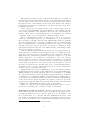
in Section 2.2 and the reference valuation π0 , the following constraints is generated by Imitator II in 2.3 seconds:
rc slow min > 2 ∗ delay + rc fast max
∧
rc fast min > 2 ∗ delay
By definition of the inverse problem, this constraint corresponds to parameter valuations having exactly the same behavior (i.e., exactly the same trace set)
as for π0 . However, there may be other parameter valuations having different
good behaviors (i.e., different good trace sets). Finding those other parameter
valuations is the purpose of the next section.
2.4
The Behavioral Cartography Algorithm
We recall here the behavioral cartography algorithm, as defined in [5]. By
iterating the above inverse method IM over all the integer points of a rectangle
V0 (of which there are a finite number), one is able to decompose (most of) the
parametric space included into V0 into behavioral tiles. Formally:
Algorithm 2: Behavioral Cartography Algorithm BC (A, V0 )
input : A PTA A, a finite rectangle V0 ⊆ RM
≥0
output: Tiling: list of tiles (initially empty)
4
repeat
select an integer point π ∈ V0 ;
if π does not belong to any tile of Tiling then
Add IM (A, π) to Tiling;
5
until Tiling contains all the integer points of V0 ;
1
2
3
Note that two tiles with distinct trace sets are necessarily disjoint. On the
other hand, two tiles with the same trace sets may overlap.
In practice, most of (the real-valued space of) V0 is covered by Tiling. Furthermore, the space covered by Tiling often largely exceeds the limits of V0
(see [5] for a sufficient condition of full coverage of the parametric space).
Partition Between Good and Bad Tiles. According to a given property
on traces one wants to check, it is possible to partition trace sets between good
and bad. Once one has decided which tiles are good and which ones are bad,
6
one can partition the rectangle V0 into a good subspace (union of good tiles)
and a bad subspace (union of bad tiles).
Advantages. First, the cartography itself does not depend on the property
one wants to check. Only the partition between good and bad tiles involves the
considered property. Moreover, the algorithm is interesting because one does
not need to compute the set of all the reachable states. On the contrary, each
call to the inverse method algorithm quickly reduces the state space by removing
the “bad” states. This allows us to overcome the state space explosion problem,
which prevents other methods, such as the computation of the whole set of
reachable states (and then the intersection with the bad states), to terminate
in practice.
Application to the Root Contention Protocol. To find other valuations of the parameters for which the system still behaves well, we compute a cartography of the Root Contention Protocol with the following V0 :
rc slow min ∈ [140, 200], rc slow max ∈ [140, 200] and delay ∈ [1, 50]. The two
other parameters remain constant, as in π0 .
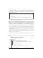
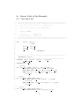
The cartography computed by Imitator II is given in Figure 1. For the
sake of clarity, we project onto delay and rc slow min. In each tile, the parameter rc slow max is only bound by the implicit constraint rc slow min ≤
rc slow max .
Note that tiles 1 and 6 are infinite towards dimension rc slow min, and all
tiles are infinite towards dimension rc slow max . Moreover, although all the
integer points within V0 are covered (from the algorithm), note that the realvalued part of V0 is not fully covered, because there are some “holes” (real-valued
zones without integer points) in the lower right corner. An example of point
which not covered by the cartography is delay = 50, rc slow min = 140.4 and
rc slow max = 141.
It can be shown that tiles 1 to 3 correspond to good tiles, whereas the
other tiles correspond to bad tiles 4 . As a consequence, the solution to the good
parameters problem for this example corresponds to the parameter valuations
included in tiles 1, 2 and 3. The corresponding constraint is the following one
(recall that rc fast min = 76 and rc fast max = 85):
2∗rc slow min > 3∗delay+170 ∧ delay < 38 ∧ rc slow min ≤ rc slow max
3
3.1
General Structure and Implementation
Inputs and Outputs
The input syntax of Imitator II to describe the network of PTAs modeling the
system is given in [7], and is very close to the HyTech syntax. Actually, all
standard HyTech files describing only PTAs (and not more general systems
4 Note that what Imitator II computes is a list of tiles as well as the associated trace
sets. We then use an external tool (here, Prism) in order to verify for each tile whether the
considered property Prop 1 is satisfied or not. Note that this step could be easily integrated
to Imitator II in automatic manner (see final remarks in Section 6).
7
rc slow min
220
210
200
190
6
180
1
170
160
5
11
14
150
4 9
2
140
3
19
12
16
7
18
8
17
130
13
10
120
15
110
100
90
80
00
10
20
30
40
50
60
70
80
90
100
delay
Figure 1: Behavioral cartography of the Root Contention Protocol according to
delay and rc slow min
like linear hybrid automata[1]) can be analyzed directly by Imitator II with
very minor changes5 .
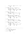
Inverse Method. When calling Imitator II to apply the inverse method algorithm, the tool takes as input two files, one describing the network of PTAs
modeling the system, and the other describing the reference valuation. As depicted in Figure 2, it synthesizes a constraint on the parameters solving the
inverse problem, as well as the corresponding trace set under a graphical form.
The description of all the parametric reachable states is also returned.
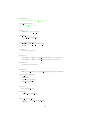
Behavioral Cartography Algorithm. When calling Imitator II to apply
the behavioral cartography algorithm, the tool takes as an input two files, one
5 An interface to accept as well files given using the PHAVer syntax is currently being
implemented.
8
Constraint K0 on
the parameters
PTA A
Imitator II
Trace set
(graphical form)
Reference
valuation π0
Figure 2: Imitator II inputs and outputs in inverse method mode
describing the network of PTAs modeling the system, and the other describing the reference rectangle, i.e., the bounds to consider for each parameter.
As depicted in Figure 3, it synthesizes a list of tiles, as well as the trace set
corresponding to each tile under a graphical form. The description of all the
parametric reachable states for each tile is also returned.
PTA A
List of tiles
Imitator II
List of trace sets
(graphical form)
Reference
rectangle V0
Figure 3: Imitator II inputs and outputs in behavioral cartography mode
3.2
Structure and Implementation
Structure. Whereas Imitator was a prototype written in Python calling
HyTech for the computation of the Post operation, Imitator II is a standalone tool written in OCaml. The Post operation has been fully implemented,
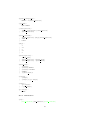
and the inverse method algorithm entirely rewritten. As depicted in Figure 4,
Imitator II makes use of an external library for manipulating convex polyhedra.
Depending on the user’s preference, Imitator II can call either the NewPolka
library, available in the Apron library [18], or the Parma Polyhedra Library
(PPL) [9]. The trace sets are output under a graphical form using the dot
module of the graph visualization software Graphviz.
Imitator II contains about 9000 lines of code, and its development took
about 6 man-months.
Imitator II (OCaml)
Apron
dot
PPL
NewPolka
Figure 4: Imitator II internal structure
9
Internal Representation. States are represented using a triple (q, v, C)
made of the current location q in each automaton, a value for each discrete
variable6 v, and a constraint C on the clocks and the parameters. In order
to optimize the test of equality between a new computed state and the set of
states computed previously, the states are stored in a hash table as follows: to
a given key (q, v) of the hash table, we associate a list of constraints C1 , . . . , Cn ,
corresponding to the n states (q, v, C1 ), . . . , (q, v, Cn ).
Note that, unlike HyTech, Imitator II uses exact arithmetics with unlimited precision.
Contrarily to HyTech which performs an a priori static composition of the
automata, thus leading to a dramatical explosion of the number of locations,
Imitator II performs an on-the-fly composition of the automata. This on-thefly composition allows to analyze bigger systems, and decrease drastically the
computation time compared to Imitator.
3.3
Features
Imitator II includes the following features:
• Reachability analysis: given a PTA A, compute the set of all the reachable
states (as it is done in tools such as, e.g., HyTech and PHAVer);
• Inverse method algorithm: given a PTA A and a reference valuation π0 ,
synthesize a constraint guaranteeing the same trace set as for A[π0 ];
• Behavioral cartography algorithm: given a PTA A and a rectangular parameter domain V0 , compute a list of tiles. Two different modes can be
considered: (1) cover all the integer points of V0 or, (2) call a given number
of times the inverse method on an integer point selected randomly within
V0 (which is interesting for rectangles containing a very big number of
integer points but few different tiles);
• Automatic generation of the trace sets, for the reachability analysis and
for both algorithms IM and BC ;
• Output of the trace sets under a graphical form.
As shown in Table 1, all those features (except the inverse method) are new
features which were not available in Imitator.
Tool
Imitator
Imitator II
Inverse Method
Yes
Yes
Cartography
Yes
Computation of traces
Yes
Graphical output
Yes
Table 1: Comparison of the features of Imitator and Imitator II
See Section 4.3.4 for the list of options available when calling Imitator II.
6 Discrete variables are syntactic sugar allowing to factorize several locations into a single one. In Imitator II, discrete variables are integer variables that can be updated using
constants or other discrete variables.
10
4
How to Use Imitator II
4.1
Installation
See the installation files available on the website for the most up-to-date information.
In short, Imitator II is written in OCaml, and makes use of the following
libraries:
• The APRON numerical abstract domain library [18], and its interface with
OCaml
• The OCaml ExtLib library (Extended Standard Library for Objective
Caml)
• The Parma Polyhedra Library (PPL) [9]
Various binaries are available on Imitator II’s Web page.
4.2
The Imitator II Input File
The syntax of the automata in Imitator II is similar to the syntax of the
automata for HyTech.
4.2.1
Variables
Discrete variables, clocks and parameters variable names must be disjoint.
The synchronization label names may be identical to other names (automata
or variables). The automata names may be identical to other names (variables
synchronization labels).
4.2.2
Parametric Timed Automata
See Appendix B.
4.2.3
Initial region and π0
See Appendix B.
4.3
Calling Imitator II
Imitator II can be used with three different modes:
1. Reachability analysis: given a PTA A, compute the whole set of reachable
states from a given initial state.
2. Inverse Method: given a PTA A and a valuation π0 of the parameters,
compute a constraint on the parameters guaranteeing the same behavior
as under π0 [4].
3. Behavioral Cartography Algorithm: given a PTA A and a rectangle V0
(bounded interval of values for each parameter), compute a cartography
of the system [5].
We detail those three modes below.
11
4.3.1
Reachability Analysis
Given a PTA A, the reachability analysis computes the whole set of reachable
states from a given initial state. The syntax in this case is the following one:
IMITATOR2 <input file> -mode reachability [options]
Note that there is no need to provide a π0 or V0 file in this case (if one is
provided, it will be ignored).
In this case, Imitator II outputs two files:
• A file <input file>.states containing the set of all the reachable states,
with their names and the associated constraint on the clocks and parameters. If one wants to generate also the constraint on the parameters only,
use the -with-parametric-log option. This file also contains the source
for the generation of the graphical file, using the dot syntax. This log file
is not generated in the case where the -no-log option is activated.
• A file <input file>.gif, which is a graphical output in the gif format,
generated using dot, corresponding to the trace set. This graphical output is not generated in the case where the -no-dot option is activated.
Note that the location and the name of those two files can be changed using
the -log-prefix option.
4.3.2
Inverse Method
Given a PTA A and a valuation π0 of the parameters, the inverse method
compute a constraint K0 on the parameters guaranteeing that, for any π |= K0 ,
the trace sets of A[π] and A[π0 ] are the same [4]. The syntax in this case is the
following one:
IMITATOR2 <input file> <pi0 file> [-mode inversemethod]
[options]
Note that the -mode inversemethod option is not necessary, since the default value for -mode is precisely inversemethod.
Note that, unlike the algorithm given in [4], at a given iteration, the π0 incompatible state is selected deterministically, for efficiency reasons. However,
the π0 -incompatible inequality within a π0 -incompatible state is selected randomly, unless the -no-random option is activated.
In this case, Imitator II outputs the resulting constraint K0 on the standard
output. Moreover, Imitator II outputs the same two files as in the reachability
analysis.
4.3.3
Cartography
Given a PTA A and a rectangle V0 (bounded interval of values for each parameter), the Behavioral Cartography Algorithm computes a cartography of the
system [5]. Two possible variants of the algorithm can be used:
1. The standard variant covers all the integer points within V0 . The syntax
in this case is the following one:
IMITATOR2 <input file> <V0 file> [-mode cover] [options]
12
2. The alternative variant calls the inverse method a certain number of times
on a random point V0 . The syntax in this case is the following one:
IMITATOR2 <input file> <V0 file> [-mode randomX] [options]
where X represents the number of random points to consider. If a point
has already been generated before, the inverse method is not called. If a
point belongs to one of the tiles computed before, the inverse method is
not called neither. Therefore, in practice, the number of tiles generated is
smaller than X.
4.3.4
Options
The options available for Imitator II are explained in the following.
-acyclic (default: false) Does not test if a new state was already encountered. In a normal use, when Imitator II encounters a new state, it checks if
it has been encountered before. This test may be time consuming for systems
with a high number of reachable states. For acyclic systems, all traces pass only
once by a given location. As a consquence, there are no cycles, so there should
be no need to check if a given state has been encountered before. This is the
main purpose of this option.
However, be aware that, even for acyclic systems, several (different) traces
can pass by the same state. In such a case, if the -acyclic option is activated,
Imitator II will compute twice the states after the state common to the two
traces. As a consequence, it is all but sure that activating this option will lead
to an increase of speed.
Note also that activating this option for non-acyclic systems may lead to an
infinite loop in Imitator II.
-debug (default: standard) Give some debugging information, that may also
be useful to have more details on the way Imitator II works. The admissible
values for -debug are given below:
nodebug Give only the resulting constraint
standard Give little information (number of steps, computation time)
low
Give little additional debugging information
medium
Give quite a lot of debugging information
high
Give much debugging information
total
Give really too much information
-inclusion (default: false) Consider an inclusion of region instead of the
equality when performing the Post operation. In other terms, when encountering a new state, Imitator II checks if the same state (same location and
same constraint) has been encountered before and, if yes, does not consider this
“new” state. However, when the -inclusion option is activated, it suffices that
a previous state with the same location and a constraint greater or equal to
the constraint of the new state has been encountered to stop the analysis. This
option corresponds to the way that, e.g., HyTech works, and suffices when one
wants to check the non-reachability of a given bad state.
-log-prefix (default: <input file>)
graphical (.gif) files.
13
Set the prefix for log (.states) and
-mode (default: inversemethod) The mode for Imitator II.
reachability Parametric reachability analysis
(see Section 4.3.1)
inversemethod Inverse method
(see Section 4.3.2)
cover
Behavioral Cartography Algorithm with full coverage
(see Section 4.3.3)
randomXX
Behavioral Cartography Algorithm with XX iterations
(see Section 4.3.3)
-no-dot (default: false)
No graphical output using dot.
-no-log (default: false)
states.
No generation of the files describing the reachable
-no-random (default: false) No random selection of the π0 -incompatible
inequality (select the first found). By default, select an inequality in a random
manner.
-post-limit <limit> (default: none) Limits the number of iterations in
the Post exploration, i.e., the depth of the traces. In the cartography mode,
this option gives a limit to each call to the inverse method.
-sync-auto-detect (default: false) Imitator II considers that all the automata declaring a given synchronization label must be able to synchronize
all together, so that the synchronization can happen. By default, Imitator II
considers that the synchronization labels declared in an automaton are those declared in the synclabs section. Therefore, if a synchronization label is declared
but never used in (at least) one automaton, this label will never be synchronized
in the execution7 .
The option -sync-auto-detect allows to detect automatically the synchronization labels in each automaton: the labels declared in the synclabs section
are ignored, and the Imitator II considers that only the labels really used in
an automaton are those considered to be declared.
-time-limit <limit> (default: none) Try to limit the execution time (the
value <limit> is given in seconds). Note that, in the current version of Imitator II, the test of time limit is performed at the end of an iteration only
(i.e., at the end of a given Post iteration). In the cartography mode, this option
represents a global time limit, not a limit for each call to the inverse method.
-timed (default: false)
program.
Add a timing information to each output of the
-with-parametric-log (default: false) For any constraint on the clocks
and the parameters in the description of the states in the log files, add the
constraint on the parameters only (i.e., eliminate clock variables).
7 In such a case, the synchronization label is actually completely removed before the execution, in order to optimize the execution, and the user is warned of this removal.
14
4.3.5
Examples of Calls
IMITATOR2 flipflop.imi -mode reachability Computes a reachability
analysis on the automata described in file flipflop.imi. Will generate files
flipflop.imi.states, containing the description of the reachable states, and
flipflop.imi.gif depicting the reachability graph.
IMITATOR2 flipflop.imi flipflop.pi0 Calls the inverse method on the automata described in file flipflop.imi, and the reference valuation π0 given in
file flipflop.pi0. The resulting constraint K0 will be given on the standard
output. Moreover, Imitator II will generate the file flipflop.imi.states,
containing the description of the (parametric) states reachable under K0 , and
the file flipflop.imi.gif depicting the reachability graph under any point
π |= K0 .
IMITATOR2 flipflop.imi flipflop.pi0 -no-dot -no-log Calls the inverse method on the automata described in file flipflop.imi, and the reference
valuation given in file flipflop.pi0. The resulting constraint will be given on
the standard output. No file will be generated.
IMITATOR2 flipflop.imi flipflop.pi0 -with-parametric-log Calls the
inverse method on the automata described in file flipflop.imi, and the reference valuation π0 given in file flipflop.pi0. The resulting constraint K0
will be given on the standard output. and Imitator II will generate the file
flipflop.imi.states, containing the description of the (parametric) states
reachable under K0 . Moveover, for any state in this file, both the constraint
on the clocks and the parameters, and the constraint on the parameters will be
given. Imitator II will also generate the file flipflop.imi.gif depicting the
reachability graph under any point π |= K0 .
IMITATOR2 SRlatch.imi SRlatch.v0 -mode cover Calls the behavioral
cartography algorithm on the automata described in file flipflop.imi, and
the rectangle V0 given in file SRlatch.v0. The algorithm will cover (at least)
all the integer points within V0 . The resulting set of tiles will be given on the
standard output. Given n the number of generated tiles (i.e., the number of
calls to the inverse method algorithm), the program will generate n files of
the form SRlatch.imi i.states (resp. n files of the form SRlatch.imi i.gif)
giving the description of the states (resp. the reachability graph) of tile i, for
i = 1, . . . , n.
IMITATOR2 SRlatch.imi SRlatch.v0 -mode random100 -no-log Calls the
behavioral cartography algorithm on the automata described in file
flipflop.imi, and the rectangle V0 given in file SRlatch.v0. The program will
call the inverse method on 100 points randomly selected within V0 . Since some
points may be generated several times, or some points may belong to previously
generated tiles (see Section 4.3.3), the number n of tiles generated will be such
that n ≤ 100. The program will generate n files of the form SRlatch.imi i.gif
giving the reachability graph of tile i, for i = 1, . . . , n.
15
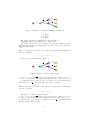
R
Q
S

Q
S
R
t↓
Figure 5: SR latch (left) and environment (right)
5
Example: SR-latch
We consider a SR-latch described in, e.g., [13], and depicted on Fig. 5 left. The
possible configurations of the latch are the following ones:
S
0
0
1
1
R
0
1
0
1
Q
latch
0
1
0
Q
latch
1
0
0
We consider an initial configuration with R = S = 1 and Q = Q = 0. As
depicted in Fig. 5, the signal S first goes down. Then, the signal R goes down
after a time t↓ .
We consider that the gate Nor 1 (resp. Nor 2 ) has a punctual parametric
delay δ1 (resp. δ2 ). Moreover, the parameter t↓ corresponds to the time duration
between the fall of S and the fall of R.
5.1
Parametric Reachability Analysis
We first perform a reachability analysis. The launch command for Imitator II
is the following one:
IMITATOR2 SRlatch.imi -mode reachability
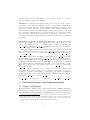
Considering this environment, the trace set of this system is given in Fig. 6,
where the states qi , i = 0, . . . , 6 correspond to the following values for each
signal:
State
q0
q1
q2
q3
q4
q5
q6
5.2
S
1
0
0
0
0
0
0
R
1
1
0
1
0
0
0
Q
0
0
0
0
0
1
0
Q
0
0
0
1
1
0
1
Behavioral Cartography Algorithm
Using Imitator II, we now perform a behavioral cartography of this system.
We consider the following rectangle V0 for the parameters:
16
Q
q0
S↓
q1
↑
R↓
q3
q2
R↓
Q
q6
↑
q4
Q↑
q5
Figure 6: Parametric reachability analysis of the SR latch
t↓ ∈ [0, 10]
δ1 ∈ [0, 10]
δ2 ∈ [0, 10]
The launch command for Imitator II is the following one:
IMITATOR2 SRlatch.imi SRlatch.v0 -mode cover
We get the following six behavioral tiles. Note that the graphical outputs,
automatically generated by Imitator II in the gif format, were rewritten in
LATEX in this document.
Tile 1. This tile corresponds to the values of the parameters verifying the
following constraint:
t↓ = δ2 ∧ δ1 = 0
The trace set of this tile is given in Fig. 7.
Q
q0
S↓
q1
↑
R↓
q3
q2
R↓
Q
q6
↑
Q↑
q4
q5
Figure 7: Trace set of tile 1 for the SR latch
↑
Since t↓ = δ2 , R↓ and Q will occur at the same time. Thus, the order of
those two events is unspecified, which explains the choice between going to q2
or q3 . When in state q2 , either Q↑ can occur (since δ1 = 0), in which case the
↑
system is stable, or Q can occur, which also leads to stability.
Tile 2. This tile corresponds to the values of the parameters verifying the
following constraint:
t↓ = δ2 ∧ δ1 > 0
The trace set of this tile is given in Fig. 8.
↑
Since t↓ = δ2 , R↓ and Q will occur at the same time. Thus, the order of
those two events is unspecified, which explains the choice between going to q2 or
↑
q3 . When in state q2 , Q↑ can not occur (since δ1 > 0), so Q occurs immediately
↓
after R , which leads to stability.
17
Q
q0
S↓
q1
↑
R↓
q3
q2
R↓
Q
q6
↑
q4
Figure 8: Trace set of tile 2 for the SR latch
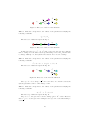
Tile 3. This tile corresponds to the values of the parameters verifying the
following constraint:
δ2 > t↓ + δ1
The trace set of this tile is given in Fig. 9.
q0
S↓
R↓
q1
q2
Q↑
q5
Figure 9: Trace set of tile 3 for the SR latch
In this case, since δ2 > t↓ + δ1 , S ↓ will occur before the gate Nor 2 has the
time to change. For the same reason, Q↑ will change before Nor 1 has the time
to change. With Q = 1, the system is now stable: Nor 1 does not change.
Tile 4. This tile corresponds to the values of the parameters verifying the
following constraint:
t↓ + δ1 = δ2 ∧ δ2 ≥ δ1 ∧ δ1 > 0
The trace set of this tile is given in Fig. 10.
q0
S↓
R↓
q1
q2
Q↑
Q
↑
q5
q4
Figure 10: Trace set of tile 4 for the SR latch
↑
Since t↓ + δ1 = δ2 , both Q↑ or Q can occur. Once one of them occured, the
system gets stable, and no other change occurs.
Tile 5. This tile corresponds to the values of the parameters verifying the
following constraint:
δ2 > t↓ ∧ t↓ + δ1 > δ2
The trace set of this tile is given in Fig. 11.
Since δ2 > t↓ , the gate Nor 2 can not change before R↓ occurs. However,
since t↓ + δ1 > δ2 , the gate Nor 2 changes before Q↑ can occur, thus leading to
↑
event Q .
18
q0
S↓
R↓
q1
q2
Q
↑
q4
Figure 11: Trace set of tile 5 for the SR latch
Tile 6. This tile corresponds to the values of the parameters verifying the
following constraint:
t↓ > δ2
The trace set of this tile is given in Fig. 12.
q0
S↓
Q
q1
↑
q3
R↓
q6
Figure 12: Trace set of tile 6 for the SR latch
↑
Since t↓ > δ2 , Q occurs before S ↓ . The system is then stable.
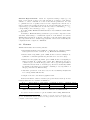
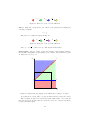
Cartography. We give in Fig. 13 the cartography of the SR latch example.
For the sake of simplicity of representation, we consider only parameters δ1 and
δ2 . Therefore, we set t↓ = 1.
δ2
4
3
5
1
2
6
δ1
Figure 13: Behavioral cartography of the SR latch according to δ1 and δ2
Note that tile 1 corresponds to a point, and tiles 2 and 4 correspond to lines.
The rectangle V0 has been represented with dashed lines. Note that all
tiles (except tile 1) are unbounded, so that they cover, not only V0 , but all the
positive real-valued plan.
19
The source code of this example is available in Appendix A.
6
Final Remarks
The tool Imitator II allows us to solve the good parameters problem for timed
automata by iterating the inverse method algorithm on the integer points of a
given rectangular parameter domain V0 . In practice, our cartography algorithm
covers not only (most of) V0 but also a significant part of the whole parametric
space beyond V0 . This is of interest to classify the behavior of the system into
good or bad for dense and unbounded values of the parameters.
Our tool has been successfully applied to various examples of asynchronous
circuits and protocols.
Future works include:
• an automatic generation of the cartography under a graphical form (so far,
only the trace sets are automatically generated under a graphical form;
the cartography itself is given under the form of a list of constraints);
• an automatic verification of the property one wants to check, e.g., by using
a tool such as Uppaal [20];
• a “dynamic” cartography, where the scale (so far, the integers) can be
refined to fill the possible holes;
• a backward analysis, i.e., considering a Pre operation instead of Post
computation in Algorithm 1;
• the reachability analysis of a given state, and the generation of a trace
from the initial state to this given state;
• the extension to hybrid systems;
• the automatic generation of the probabilities of a given property in
the probabilistic framework, without the use of an external tool (e.g.,
Prism [16])
• the automatic generation of the “next point” not covered by Tiling without testing all the integer points (note that a random generation of points
is already implemented);
• the possibility to compute several tiles in parallel in the cartography algorithm;
• a user-friendly graphical interface;
• the possibility to save and load sets of states.
Acknowledgments. Emmanuelle Encrenaz and Laurent Fribourg have been
great contributors of Imitator II, on a theoretical point of view, and to find
applications both from the literature and real case studies. Abdelrezzak Bara
provided several examples from the hardware literature. Jeremy Sproston provided examples from the probabilistic community. Bertrand Jeannet has been
of great help on the installation part, and the linking with Apron [18]. Ulrich K¨
uhne started to improve Imitator II, and added the link with PPL.
20
References
[1] R. Alur, C. Courcoubetis, T.A. Henzinger, and P.H. Ho. Hybrid automata:
An algorithmic approach to the specification and verification of hybrid
systems. In Hybrid Systems, pages 209–229, 1992.
[2] R. Alur and D. L. Dill. A theory of timed automata. TCS, 126(2):183–235,
1994.
[3] R. Alur, T.A. Henzinger, and M. Y. Vardi. Parametric real-time reasoning.
In STOC ’93, pages 592–601. ACM, 1993.
´ Andr´e, T. Chatain, E. Encrenaz, and L. Fribourg. An inverse method
[4] E.
for parametric timed automata. International Journal of Foundations of
Computer Science, 20(5):819–836, 2009.
´ Andr´e and L. Fribourg. Behavioral cartography of timed automata. In
[5] E.
RP’10, LNCS. Springer, 2010. To appear.
´ Andr´e, L. Fribourg, and J. Sproston. An extension of the inverse method
[6] E.
to probabilistic timed automata. In AVoCS’09, volume 23 of Electronic
Communications of the EASST, 2009.
´
[7] Etienne
Andr´e. Imitator II web page. http://www.lsv.ens-cachan.fr/
andre/IMITATOR2.
~
´
[8] Etienne
Andr´e. IMITATOR: A tool for synthesizing constraints on timing
bounds of timed automata. In ICTAC’09, volume 5684 of LNCS, pages
336–342. Springer, 2009.
[9] R. Bagnara, P. M. Hill, and E. Zaffanella. The Parma Polyhedra Library:
Toward a complete set of numerical abstractions for the analysis and verification of hardware and software systems. Science of Computer Programming, 72(1–2):3–21, 2008.
[10] C. Baier and J.-P. Katoen. Principles of Model Checking. The MIT Press,
2008.
[11] E. M. Clarke, O. Grumberg, S. Jha, Y. Lu, and H. Veith. Counterexampleguided abstraction refinement. In CAV ’00, pages 154–169. Springer-Verlag,
2000.
[12] G. Frehse, S.K. Jha, and B.H. Krogh. A counterexample-guided approach
to parameter synthesis for linear hybrid automata. In HSCC ’08, volume
4981 of LNCS, pages 187–200. Springer, 2008.
[13] D. Harris and S. Harris. Digital Design and Computer Architecture. Morgan
Kaufmann Publishers Inc., San Francisco, CA, USA, 2007.
[14] T.A. Henzinger, P.H. Ho, and H. Wong-Toi. Hytech: A model checker for
hybrid systems. Software Tools for Technology Transfer, 1:460–463, 1997.
[15] T.A. Henzinger and H. Wong-Toi. Using HyTech to synthesize control
parameters for a steam boiler. In Formal Methods for Industrial Applications: Specifying and Programming the Steam Boiler Control, LNCS 1165.
Springer-Verlag, 1996.
21
[16] A. Hinton, M. Kwiatkowska, G. Norman, and D. Parker. PRISM: A tool
for automatic verification of probabilistic systems. In TACAS’06, volume
3920 of LNCS, pages 441–444. Springer, 2006.
[17] T.S. Hune, J.M.T. Romijn, M.I.A. Stoelinga, and F.W. Vaandrager. Linear parametric model checking of timed automata. Journal of Logic and
Algebraic Programming, 2002.
[18] B. Jeannet and A. Min´e. Apron: A library of numerical abstract domains
for static analysis. In CAV ’09, volume 5643 of LNCS, pages 661–667.
Springer, 2009.
[19] M. Kwiatkowska, G. Norman, and J. Sproston. Probabilistic model checking of deadline properties in the IEEE 1394 FireWire root contention protocol. Formal Aspects of Computing, 14(3):295–318, 2003.
[20] K. G. Larsen, P. Pettersson, and W. Yi. Uppaal in a nutshell. International
Journal on Software Tools for Technology Transfer, 1(1-2):134–152, 1997.
22
A
A.1
1
2
3
4
5
6
7
8
9
10
11
12
Source Code of the Example
Main Input File
−−∗∗∗∗∗∗∗∗∗∗∗∗∗∗∗∗∗∗∗∗∗∗∗∗∗∗∗∗∗∗∗∗∗∗∗∗∗∗∗∗∗∗∗∗∗∗∗∗∗∗∗∗∗∗∗∗∗∗∗∗ − −
−−∗∗∗∗∗∗∗∗∗∗∗∗∗∗∗∗∗∗∗∗∗∗∗∗∗∗∗∗∗∗∗∗∗∗∗∗∗∗∗∗∗∗∗∗∗∗∗∗∗∗∗∗∗∗∗∗∗∗∗∗ − −
−−
Laboratoire S p e c i f i c a t i o n et V e r i f i c a t i o n
−−
−−
Race on a d i g i t a l c i r c u i t (SR Latch )
−−
−−
E t i e n n e ANDRE
−−
−−
Created :
2010/03/19
−−
Last m o d i f i e d : 2010/03/24
−−∗∗∗∗∗∗∗∗∗∗∗∗∗∗∗∗∗∗∗∗∗∗∗∗∗∗∗∗∗∗∗∗∗∗∗∗∗∗∗∗∗∗∗∗∗∗∗∗∗∗∗∗∗∗∗∗∗∗∗∗ − −
−−∗∗∗∗∗∗∗∗∗∗∗∗∗∗∗∗∗∗∗∗∗∗∗∗∗∗∗∗∗∗∗∗∗∗∗∗∗∗∗∗∗∗∗∗∗∗∗∗∗∗∗∗∗∗∗∗∗∗∗∗ − −
13
14
15
var
ckNor1 , ckNor2 , s
: clock ;
16
17
18
19
20
dNor1 l , dNor1 u ,
dNor2 l , dNor2 u ,
t down
: parameter ;
21
22
23
24
25
26
27
28
−−∗∗∗∗∗∗∗∗∗∗∗∗∗∗∗∗∗∗∗∗∗∗∗∗∗∗∗∗∗∗∗∗∗∗∗∗∗∗∗∗∗∗∗∗∗∗∗∗∗∗∗∗∗∗∗∗∗∗∗∗ − −
automaton norGate1
−−∗∗∗∗∗∗∗∗∗∗∗∗∗∗∗∗∗∗∗∗∗∗∗∗∗∗∗∗∗∗∗∗∗∗∗∗∗∗∗∗∗∗∗∗∗∗∗∗∗∗∗∗∗∗∗∗∗∗∗∗ − −
synclabs : R Up , R Down , overQ Up , overQ Down ,
Q Up , Q Down ;
i n i t i a l l y Nor1 110 ;
29
30
31
32
33
34
−− UNSTABLE
loc Nor1 000 : while ckNor1 <= dNor1 u wait {}
when True sync R Up do {} goto Nor1 100 ;
when True sync overQ Up do {} goto Nor1 010 ;
when ckNor1 >= d N o r 1 l sync Q Up do {} goto
Nor1 001 ;
35
36
37
38
39
−− STABLE
loc Nor1 001 : while True wait {}
when True sync R Up do { ckNor1 ’ = 0} goto
Nor1 101 ;
when True sync overQ Up do { ckNor1 ’ = 0} goto
Nor1 011 ;
40
41
42
43
−− STABLE
loc Nor1 010 : while True wait {}
when True sync R Up do {} goto Nor1 110 ;
23
44
when True sync overQ Down do { ckNor1 ’ = 0} goto
Nor1 000 ;
45
46
47
48
49
50
−− UNSTABLE
loc Nor1 011 : while ckNor1 <= dNor1 u wait {}
when True sync R Up do { ckNor1 ’ = 0} goto
Nor1 111 ;
when True sync overQ Down do {} goto Nor1 001 ;
when ckNor1 >= d N o r 1 l sync Q Down do {} goto
Nor1 010 ;
51
52
53
54
55
−− STABLE
loc Nor1 100 : while True wait {}
when True sync R Down do { ckNor1 ’ = 0} goto
Nor1 000 ;
when True sync overQ Up do {} goto Nor1 110 ;
56
57
58
59
60
61
−− UNSTABLE
loc Nor1 101 : while ckNor1 <= dNor1 u wait {}
when True sync R Down do {} goto Nor1 001 ;
when True sync overQ Up do { ckNor1 ’ = 0} goto
Nor1 111 ;
when ckNor1 >= d N o r 1 l sync Q Down do {} goto
Nor1 100 ;
62
63
64
65
66
−− STABLE
loc Nor1 110 : while True wait {}
when True sync R Down do {} goto Nor1 010 ;
when True sync overQ Down do {} goto Nor1 100 ;
67
68
69
70
71
72
−− UNSTABLE
loc Nor1 111 : while ckNor1 <= dNor1 u wait {}
when True sync R Down do { ckNor1 ’ = 0} goto
Nor1 011 ;
when True sync overQ Down do { ckNor1 ’ = 0} goto
Nor1 101 ;
when ckNor1 >= d N o r 1 l sync Q Down do {} goto
Nor1 110 ;
73
74
end −− norGate1
75
76
77
78
79
80
81
82
83
−−∗∗∗∗∗∗∗∗∗∗∗∗∗∗∗∗∗∗∗∗∗∗∗∗∗∗∗∗∗∗∗∗∗∗∗∗∗∗∗∗∗∗∗∗∗∗∗∗∗∗∗∗∗∗∗∗∗∗∗∗ − −
automaton norGate2
−−∗∗∗∗∗∗∗∗∗∗∗∗∗∗∗∗∗∗∗∗∗∗∗∗∗∗∗∗∗∗∗∗∗∗∗∗∗∗∗∗∗∗∗∗∗∗∗∗∗∗∗∗∗∗∗∗∗∗∗∗ − −
synclabs : Q Up , Q Down , S Up , S Down ,
overQ Up , overQ Down ;
−− i n i t i a l l y Nor2 110 ;
i n i t i a l l y Nor2 001 ;
84
24
85
86
87
88
89
−− UNSTABLE
loc Nor2 000 : while ckNor2 <= dNor2 u wait {}
when True sync Q Up do {} goto Nor2 100 ;
when True sync S Up do {} goto Nor2 010 ;
when ckNor2 >= d N o r 2 l sync overQ Up do {} goto
Nor2 001 ;
90
91
92
93
94
−− STABLE
loc Nor2 001 : while True wait {}
when True sync Q Up do { ckNor2 ’ = 0} goto
Nor2 101 ;
when True sync S Up do { ckNor2 ’ = 0} goto
Nor2 011 ;
95
96
97
98
99
−− STABLE
loc Nor2 010 : while True wait {}
when True sync Q Up do {} goto Nor2 110 ;
when True sync S Down do { ckNor2 ’ = 0} goto
Nor2 000 ;
100
101
102
103
104
105
−− UNSTABLE
loc Nor2 011 : while ckNor2 <= dNor2 u wait {}
when True sync Q Up do { ckNor2 ’ = 0} goto
Nor2 111 ;
when True sync S Down do {} goto Nor2 001 ;
when ckNor2 >= d N o r 2 l sync overQ Down do {}
goto Nor2 010 ;
106
107
108
109
110
−− STABLE
loc Nor2 100 : while True wait {}
when True sync Q Down do { ckNor2 ’ = 0} goto
Nor2 000 ;
when True sync S Up do {} goto Nor2 110 ;
111
112
113
114
115
116
−− UNSTABLE
loc Nor2 101 : while ckNor2 <= dNor2 u wait {}
when True sync Q Down do {} goto Nor2 001 ;
when True sync S Up do { ckNor2 ’ = 0} goto
Nor2 111 ;
when ckNor2 >= d N o r 2 l sync overQ Down do {}
goto Nor2 100 ;
117
118
119
120
121
−− STABLE
loc Nor2 110 : while True wait {}
when True sync Q Down do {} goto Nor2 010 ;
when True sync S Down do {} goto Nor2 100 ;
122
123
124
−− UNSTABLE
loc Nor2 111 : while ckNor2 <= dNor2 u wait {}
25
125
126
127
when True sync Q Down do { ckNor2 ’ = 0} goto
Nor2 011 ;
when True sync S Down do { ckNor2 ’ = 0} goto
Nor2 101 ;
when ckNor2 >= d N o r 2 l sync overQ Down do {}
goto Nor2 110 ;
128
129
end −− norGate2
130
131
132
133
134
135
136
−−∗∗∗∗∗∗∗∗∗∗∗∗∗∗∗∗∗∗∗∗∗∗∗∗∗∗∗∗∗∗∗∗∗∗∗∗∗∗∗∗∗∗∗∗∗∗∗∗∗∗∗∗∗∗∗∗∗∗∗∗ − −
automaton env
−−∗∗∗∗∗∗∗∗∗∗∗∗∗∗∗∗∗∗∗∗∗∗∗∗∗∗∗∗∗∗∗∗∗∗∗∗∗∗∗∗∗∗∗∗∗∗∗∗∗∗∗∗∗∗∗∗∗∗∗∗ − −
synclabs : R Down , R Up , S Down , S Up ;
i n i t i a l l y env 11 ;
137
138
139
140
−− ENVIRONMENT : f i r s t S then R a t c o n s t a n t time
loc e n v 1 1 : while True wait {}
when True sync S Down do { s ’ = 0} goto e n v 1 0 ;
141
142
143
loc e n v 1 0 : while s <= t down wait {}
when s = t down sync R Down do {} goto e n v f i n a l ;
144
145
loc e n v f i n a l : while True wait {}
146
147
end −− env
148
149
150
151
−−∗∗∗∗∗∗∗∗∗∗∗∗∗∗∗∗∗∗∗∗∗∗∗∗∗∗∗∗∗∗∗∗∗∗∗∗∗∗∗∗∗∗∗∗∗∗∗∗∗∗∗∗∗∗∗∗∗∗∗∗ − −
−− ANALYSIS
−−∗∗∗∗∗∗∗∗∗∗∗∗∗∗∗∗∗∗∗∗∗∗∗∗∗∗∗∗∗∗∗∗∗∗∗∗∗∗∗∗∗∗∗∗∗∗∗∗∗∗∗∗∗∗∗∗∗∗∗∗ − −
152
153
var i n i t : region ;
154
155
156
157
158
159
160
161
162
i n i t := True
−−−−−−−−−−−−−−−−−−−−−−−−−−−−−−−−−−−−−−−−−−−−−−−−−−−−−−−−−−−−
−− INITIAL LOCATIONS
−−−−−−−−−−−−−−−−−−−−−−−−−−−−−−−−−−−−−−−−−−−−−−−−−−−−−−−−−−−−
−− S and R down
& loc [ norGate1 ] = Nor1 100
& loc [ norGate2 ] = Nor2 010
& loc [ env ]
= env 11
163
164
165
166
167
168
169
−−−−−−−−−−−−−−−−−−−−−−−−−−−−−−−−−−−−−−−−−−−−−−−−−−−−−−−−−−−−
−− INITIAL CONSTRAINTS
−−−−−−−−−−−−−−−−−−−−−−−−−−−−−−−−−−−−−−−−−−−−−−−−−−−−−−−−−−−−
& ckNor1
= 0
& ckNor2
= 0
& s
= 0
170
171
& d N o r 1 l >= 0
26
& d N o r 2 l >= 0
172
173
& d N o r 1 l <= dNor1 u
& d N o r 2 l <= dNor2 u
174
175
176
;
A.2
1
2
3
4
5
6
7
8
V0 File
−−−−−−−−−−−−−−−−−−−−−−−−−−−−−−−−−−−−−−−−−−−−−−−−−−−−−−−−−−−−
−− V0
−−−−−−−−−−−−−−−−−−−−−−−−−−−−−−−−−−−−−−−−−−−−−−−−−−−−−−−−−−−−
& dNor1 l
= 3
= 3 . . 20
& dNor1 u
& dNor2 l
= 5
= 5 . . 20
& dNor2 u
& t down
= 10
27
B
Complete Grammar
B.1
Grammar of the Input File
Imitator II input is described by the following grammar. Non-terminals appear
within angled parentheses. A non-terminal followed by two colons is defined by
the list of immediately following non-blank lines, each of which represents a
legal expansion. Input characters of terminals appear in typewritter font. The
meta symbol denotes the empty string.
The text in green is not taken into account by Imitator II, but is allowed
(or sometimes necessary) in order to allow the compatibility with HyTech files.
himitator inputi ::
hautomata descriptionsi hiniti
We define each of those two components below.
B.1.1
Automata Descriptions
hautomata descriptionsi ::
hdeclarationsi hautomatai
hdeclarationsi ::
var hvar listsi
hvar listsi ::
hvar listi : hvar typei ; hvar listsi
| hvar listi ::
<name>
| <name> , hvar listi
hvar typei ::
clock
| discrete
| parameter
hautomatai ::
hautomatoni hautomatai
| hautomatoni ::
automaton <name> hprologi hlocationsi end
hprologi ::
hinitializationi hsync labelsi
| hsync labelsi hinitializationi
| hsync labelsi
28
hinitializationi ::
initially <name> hstate initializationi ;
hstate initializationi ::
& hconvex predicatei
| hprologi ::
synclabs : hsync var listi ;
hsync var listi ::
hsync var nonempty listi
| hsync var nonempty listi ::
<name> , hsync var nonempty listi
| <name>
hlocationsi ::
hlocationi hlocationsi
| hlocationsi ::
loc <name> : while hconvex predicatei wait () htransitionsi
| loc <name> : while hconvex predicatei wait htransitionsi
htransitionsi ::
htransitioni htransitionsi
| htransitioni ::
when hconvex predicatei hupdate synchronizationi goto <name> ;
hupdate synchronizationi ::
hupdatesi
| hsyn label i
| hupdatesi hsyn label i
| hsyn label i hupdatesi
| hupdatesi ::
do ( hupdate listi )
hupdate listi ::
hupdate nonempty listi
| hupdate nonempty listi ::
hupdatei , hupdate nonempty listi
| hupdatei
29
hupdate nonempty listi ::
<name> ’ = hlinear expressioni
hsyn label i ::
sync <name>
hconvex predicatei ::
hlinear constrainti & hconvex predicatei
| hlinear constrainti
hlinear constrainti ::
hlinear expressioni hrelopi hlinear expressioni
| True
| False
hrelopi ::
<
| <=
| =
| >=
| >
hlinear expressioni ::
hlinear termi
| hlinear expressioni + hlinear termi
| hlinear expressioni - hlinear termi
hlinear termi ::
hrational i
| hrational i <name>
| hrational i * <name>
| <name>
| ( hlinear termi )
hrational i ::
hinteger i
| hinteger i / hpos integer i
hinteger i ::
hpos integer i
| - hpos integer i
hpos integer i ::
<int>
B.1.2
Initial State
hiniti ::
hinit declarationi hinit definitioni hreach command i
30
hinit declarationi ::
var init : region ;
| hreach command i ::
print ( reach forward from init endreach ) ;
| hinit definitioni ::
init := hregion expressioni ;
hregion expressioni ::
hstate predicatei
| ( hregion expressioni )
| hregion expressioni & hregion expressioni
hstate predicatei ::
loc [ <name> ] = <name>
| hlinear constrainti
B.2
Reserved Words
The following words are keywords and cannot be used as names for automata,
variables, synchronization labels or locations.
and, automaton, clock, discrete, do, end, endreach, False, forward,
from, goto, if, in, init, initially, loc, locations, not, or, parameter,
print, reach, region, sync, synclabs, True, var, wait, when, while
31