Download Morpheus User Reference Manual

Morpheus
User manual
Walter de Back and Jörn Starruß
Center for Information Services and High Performance Computing
Technische Universität Dresden, 01062 Dresden, Germany
http://imc.zih.tu-dresden.de/wiki/morpheus
Disclaimer
Non-commercial use: Morpheus (the Software) is distributed for academic use
and cannot be used for commercial gain without explicitly written agreement by the
Developers. No warranty: The Software is provided "as is" without warranty of any
kind, either express or implied, including without limitation any implied warranties
of condition, uninterrupted use, merchantability, fitness for a particular purpose, or
non-infringement. No liability: The Developers do not accept any liability for any
direct, indirect, incidential, special, exemplary or consequential damages arising in
any way out of the use of the Software.
This manual describes Morpheus version 1.1.0 (revision 866).
Development of Morpheus was supported by the German Ministry for Education
and Research (BMBF) through grants 0315734 and 0316169.
Department for Innovative Methods of Computing
Center for Information Services and High Performance Computing
Technische Universität Dresden, 01062 Dresden, Germany
http://imc.zih.tu-dresden.de/imc/
Contents
Contents
i
1 Introduction
1.1 About Morpheus . . . .
1.1.1 Software . . . .
1.1.2 Usability . . . .
1.1.3 Developers . . .
1.2 About this manual . . .
1.2.1 Margin images .
1.2.2
.
.
.
.
.
.
.
.
.
.
.
.
.
.
.
.
.
.
.
.
.
.
.
.
.
.
.
.
.
.
.
.
.
.
.
.
.
.
.
.
.
.
.
.
.
.
.
.
.
.
.
.
.
.
.
.
.
.
.
.
.
.
.
.
.
.
.
.
.
.
.
.
.
.
.
.
.
.
.
.
.
.
.
.
.
.
.
.
.
.
.
.
.
.
.
.
.
.
.
.
.
.
.
.
.
.
.
.
.
.
.
.
.
.
.
.
.
.
.
.
.
.
.
.
.
.
.
.
.
.
.
.
.
1
1
1
2
3
3
3
3
.
.
.
.
.
.
.
.
.
.
.
Status and error messages .
Job queue and archive . .
Simulation output . . . . .
.
.
.
.
.
.
.
.
.
.
.
.
.
.
.
.
.
.
.
.
.
.
.
.
.
.
.
.
.
.
.
.
.
.
.
.
.
.
.
.
.
.
.
.
.
.
.
.
.
.
.
.
.
.
.
.
.
.
.
.
.
.
.
.
.
.
.
.
.
.
.
.
.
.
.
.
.
.
.
.
.
.
.
.
.
.
.
.
.
.
.
.
.
.
.
.
.
.
.
.
.
.
.
.
.
.
.
.
.
.
.
.
.
.
.
.
.
.
.
.
.
.
.
.
.
.
.
.
.
.
.
.
.
.
.
.
.
.
.
.
.
.
.
.
.
.
.
.
.
.
.
.
.
.
.
.
.
.
.
.
.
.
.
.
.
.
.
.
.
.
.
.
.
.
.
.
.
.
.
.
.
.
.
.
.
.
.
.
.
.
.
.
.
.
.
.
.
.
.
.
.
.
.
.
.
.
.
.
.
.
.
.
.
.
.
.
.
.
.
.
.
.
.
.
.
.
.
.
.
.
.
.
.
.
.
.
.
.
.
.
.
.
.
.
.
.
.
.
.
.
.
.
.
.
.
.
.
.
.
.
.
.
.
.
.
.
.
.
.
.
.
.
.
.
.
.
.
.
.
.
.
.
.
.
.
.
.
.
.
.
.
.
.
.
.
.
.
.
.
.
.
.
.
.
.
.
.
.
.
.
.
.
.
.
.
.
.
.
.
.
.
.
.
.
.
.
.
.
.
.
.
.
.
.
.
.
.
.
.
.
.
.
.
.
.
.
.
.
.
.
.
.
.
.
5
5
6
6
6
6
6
7
7
7
7
7
8
8
8
10
10
11
11
13
13
.
.
.
.
.
.
More information .
.
.
.
.
.
.
.
.
.
.
.
.
.
.
.
.
.
.
.
.
.
2 Graphical user interface
2.1 Model construction and editing
2.1.1 Examples . . . . . . . .
2.1.2 Documents panel . . . .
2.1.3 Element editor . . . . .
2.1.4 Attribute editor . . . . .
2.1.5 Expression editor . . . .
2.1.6 Documentation . . . . .
2.1.7 Clipboard . . . . . . . .
2.1.8 Fixboard . . . . . . . .
2.2 Simulation and results . . . . .
2.2.1 Simulation execution . .
2.2.2
2.2.3
2.2.4
2.2.5
2.2.6
2.3
Restoring and checkpointing
SBML import . . . . . . . .
Parameter sweeps . . . . . . . . .
2.3.1 Multiple parameters . . . . .
2.3.2 Simulation and results . . .
2.3.3 Restoring parameter sweeps .
i
ii
Contents
3 Model formalisms
3.1 The System construct . . . . . . . . .
3.2 Differential equations . . . . . . . . .
3.2.1 Finite difference solvers . . . . .
3.2.2 Stochastic differential equations .
3.2.3 Delay differential equations . . .
3.2.4 Initial condition . . . . . . . . .
3.3 Reaction-diffusion models . . . . . . .
3.3.1 Diffusion . . . . . . . . . . . .
3.3.2 Boundary conditions . . . . . .
3.3.3 Initial condition . . . . . . . . .
3.4 Cellular Potts model . . . . . . . . . .
3.4.1 Modified Metropolis kinetics . .
3.4.2 Stepper . . . . . . . . . . . . .
3.4.3 Neighborhood . . . . . . . . . .
3.5
.
.
.
.
.
.
.
.
.
.
.
.
.
.
.
.
.
.
.
.
.
.
.
.
.
.
.
.
.
.
.
.
.
.
.
.
.
.
.
.
.
.
.
.
.
.
.
.
.
.
.
.
.
.
.
.
.
.
.
.
.
.
.
.
.
.
.
.
.
.
3.4.4
Monte Carlo Step (MCS) and time scaling
3.4.5
Cell shape, interaction and motility . . . .
3.4.6 Initial condition of spatial configuration . .
Auxiliary model formalisms . . . . . . . . . . .
4 Model description language
4.1 Declarative . . . . . . .
4.2 Domain-specific . . . . .
4.3 Encapsulation . . . . . .
4.4 Two-tiered architecture .
4.4.1 XML . . . . . . .
4.4.2 Symbols . . . . .
4.5 Mathematical constructs
4.6 XML schema . . . . . .
.
.
.
.
.
.
.
.
.
.
.
.
.
.
.
.
.
.
.
.
.
.
.
.
.
.
.
.
.
.
.
.
.
.
.
.
.
.
.
.
.
.
.
.
.
.
.
.
.
.
.
.
.
.
.
.
.
.
.
.
.
.
.
.
5 Model integration
5.1 Spatial mapping . . . . . . . . . . . . .
5.1.1 Automated mapping . . . . . . .
5.1.2 Explicit mapping with Reporters .
5.2 Scheduling . . . . . . . . . . . . . . . .
5.2.1 Simulation schedule . . . . . . . .
5.2.2 Scheduling update order . . . . .
5.2.3 Update interval . . . . . . . . .
.
.
.
.
.
.
.
.
.
.
.
.
.
.
.
.
.
.
.
.
.
.
.
.
.
.
.
.
.
.
.
.
.
.
.
.
.
.
.
.
.
.
.
.
.
.
.
.
.
.
.
.
.
.
.
.
.
.
.
.
.
.
.
.
.
.
.
.
.
.
.
.
.
.
.
.
.
.
.
.
.
.
.
.
.
.
.
.
.
.
.
.
.
.
.
.
.
.
.
.
.
.
.
.
.
.
.
.
.
.
.
.
.
.
.
.
.
.
.
.
.
.
.
.
.
.
.
.
.
.
.
.
.
.
.
.
.
.
.
.
.
.
.
.
.
.
.
.
.
.
.
.
.
.
.
.
.
.
.
.
.
.
.
.
.
.
.
.
.
.
.
.
.
.
.
.
.
.
.
.
.
.
.
.
.
.
.
.
.
.
.
.
.
.
.
.
.
.
.
.
.
.
.
.
.
.
.
.
.
.
.
.
.
.
.
.
.
.
.
.
.
.
.
.
.
.
.
.
.
.
.
.
.
.
.
.
.
.
.
.
15
15
15
16
16
17
17
17
18
18
18
19
19
20
20
20
21
22
23
.
.
.
.
.
.
.
.
.
.
.
.
.
.
.
.
.
.
.
.
.
.
.
.
.
.
.
.
.
.
.
.
.
.
.
.
.
.
.
.
.
.
.
.
.
.
.
.
.
.
.
.
.
.
.
.
.
.
.
.
.
.
.
.
.
.
.
.
.
.
.
.
.
.
.
.
.
.
.
.
25
25
25
26
26
26
27
28
28
.
.
.
.
.
.
.
33
33
34
34
34
34
36
36
.
.
.
.
.
.
.
.
.
.
.
.
.
.
.
.
.
.
.
.
.
.
.
.
.
.
.
.
.
.
.
.
.
.
.
.
.
.
.
.
.
.
.
.
.
.
.
.
.
.
.
.
.
.
.
.
.
.
.
.
.
.
.
1
Introduction
1.1
About Morpheus
Morpheus is a modeling and simulation environment for the study of multiscale
multicellular systems. It supports the simulation of discrete cell-based models as
well as ordinary differential equations and reaction-diffusion systems and facilitates
the integration of these models into multiscale models. It allows users to construct
and simulate models of gene regulation, signaling pathways, tissue patterning and
morphogenesis and explore the effects of multiscale feedbacks between these processes.
1.1.1
Software
Morpheus is a self-contained application that covers the workflow from model
construction to simulation and data analysis. Internally, it consists of two standalone components: a graphical user interface (morpheus-gui) and a simulator
(morpheus). The graphical user interface provides tools for model editing, job
execution and archiving and it generates XML-based model descriptions based on
user-specified models. The simulator takes these model description files as input
to perform numerical simulation and generate data output and visualization. The
simulator can also be used from the command line interface.
1.1.1.1
Download and installation
Morpheus is available as binary package for all major operating systems. These
can be downloaded from the download page of the Morpheus website.
For Linux, Morpheus is available as a Debian package (.deb) that can be
installed using the default package manager. For other Linux distributions, these
packages can be converted using tools such as alien.
For Mac OSX 10.6 or higher, Morpheus is distributed as an Apple disk image
(.dmg) containing the application bundle (.app). Installing Morpheus.app is done
by dragging the app into Applications, as usual. It also contains a Gnuplot.app
required for data visualization, to be installed in the same way.
For MS Windows XP or higher, Morpheus uses an installer that guides the user
through the installation process. Gnuplot for windows should be installed separately
for which a recent version can be downloaded from the gnuplot sourceforge website.
1
2
Introduction
1.1.1.2
External software
Morpheus is implemented in C++ and Qt and depends on a number of external libraries and software packages. The simulator (morpheus) is implemented in
C++. It uses XMLParser to read model description files and write simulation states
(checkpointing). Pseudo-random numbers are generated using Mersenne Twister
19937 from the C++11 standard library. Mathematical expressions are parsed and
evaluated using the math parser library muparser. TIFF image stacks are read and
written using libTIFF. For data visualization, it depends on the graphing utility
Gnuplot and its C interface. Morpheus uses openMP for shared-memory parallel
processing.
The graphical user interface (morpheus-gui) is implemented in the crossplatform framework Qt/C++. It uses a SQLite database to store an archive of
jobs and parameter sweeps. It depends on libSSH for secure communication to remote high performance computing resources for remote job submission (ssh) and
synchronization of simulation results (sftp). Furthermore, it depends on libSBML
to import biochemical network models written in SBML format.
1.1.2
Usability
Improving usability and transparency of computational tools in multicellular systems biology is a prime objective in the design of Morpheus. This widens the
audience from computational experts to more biologically trained students and
researchers within this multi-disciplinary field and it can accelerate research by
facilitating rapid development of new hypotheses into computational models and
simulation results. Ultimately, it is required to streamline the scientific workflow
in the face of the growing complexity of computational models in systems biology.
The usability and workflow management in Morpheus is most tangible in the
graphical user interface with its tools for model construction, simulation, batch
processing and archiving. However, it also extends into the modular design of the
model formalisms, generating the flexibility to construct a range of auxiliary model
formalisms. Moreover, the domain-specific language that Morpheus uses for model
description separates the process of modeling from its numerical implementation
and allows users to construct complex models in a transparent fashion.
1.1.2.1
Target audience
Morpheus is aimed at researchers and students interested in mathematical modeling
of multicellular systems. Its use does not presuppose knowledge of computational
modeling or programming. It is suitable for anyone with basic knowledge of mathematical modeling of biological systems including researchers and students with a
background in biology, mathematics, physics and related fields.
1.1.2.2
Limitations
Morpheus is not an advanced solver for ordinary differential equations or reactiondiffusion systems. The use of explicit forward solver methods precludes the sim-
1.2. About this manual
ulation of stiff systems, and the use of fixed time stepping methods requires the
specification of reasonable time-steps by the user to ensure numerical stability under acceptable computational performance. The current version does not support
solving partial differential equations with spatial derivatives other than the most
commonly used second order and thereby excludes the simulation of e.g. advective
terms.
1.1.3
Developers
Morpheus has been developed by Jörn Starruß, Walter de Back and others in the
group of Prof. Andreas Deutsch at the Center for Information Services and High
Performance Computing (ZIH) at the Technische Universität Dresden.
1.2
About this manual
This manual provides information on the main functionalities of the graphical user
interface (chapter 2), the core model formalisms it implements (chapter 3), the
domain-specific language in which Morpheus models are expressed (chapter 4) and
the methods for model integration of the various formalisms (chapter 5).
The manual does not provide an extensive list of descriptions of features or
model components. For documentation on individual model elements, users are
refered to the Documentation panel in the graphical user interface (see section
2.1.6 and figure 2.1).
It intends to concisely describe Morpheus to a degree that is relevant for constructing models, performing simulation experiments and understanding how simulation results are achieved.
1.2.1
Margin images
Images in the page margins refer to example models that are associated with
the text and contain hyperlinks to the example website. The example models
illustrate the main modeling features of Morpheus, introduce the model description
language, and can be used as templates for new models. These example models
are embedded in the application (see 2.1.1) and are described on the website (see
figure 5.1).
1.2.2
1.2.2.1
More information
Documentation in GUI
Further documentation on individual elements of a Morpheus model is available
in the graphical user interface in the Documentation panel (see section 2.1.6 and
figure 2.1).
3
4
Introduction
1.2.2.2
Website
The Morpheus website provides additional up-to-date information. It presents a
growing number of example models that represent common use cases. The website
also answers frequently asked questions, mentions how to submit bug reports,
presents a comparison to related software and a detailed performance analysis.
Published articles on Morpheus and an up-to-date list of research papers in
which the software has been used are listed on the publication page. When publishing results that were obtained with the help of Morpheus, please cite the article
on Morpheus as indicated on the publication page. This helps to maintain Morpheus and support its further development.
The URL of the website is: http://imc.zih.tu-dresden.de/wiki/morpheus.
2
Graphical user interface
The graphical user interface (GUI) provides tools to construct and edit models,
execute simulations, browse results and perform parameter sweeps.
2.1
Model construction and editing
The GUI provides a series of editing tools that facilitate the construction and
modification of computational models and performs validation of the generated
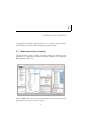
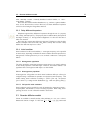
XML models (see figure 2.1).
2.1.1
2.1.5
2.1.2
2.1.8
2.1.3
2.1.6
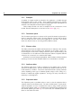
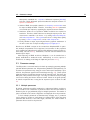
Figure 2.1: Editor view. This view is opened when selecting an element in the Documents
panel. Numbers correspond to sections in the text.
5
6
Graphical user interface
2.1.1
Examples
A number of example models is included in the application, accessible through
the Examples menu in main toolbar. These examples demonstrate key features
of Morpheus, show diverse use cases and modeling approaches and illustrate all
elements of the Morpheus model description language.
These example models can serve as templates for the construction of new
models. Detailed descriptions can be found on the website (fig. 5.1).
2.1.2
Documents panel
The Documents panel gives an overview of the opened documents and provides a
means to switch the current model. The main elements of each model are shown
and can be edited via the context menu (right-click or ctrl-click). The context
menu also allows the user to view the generated XML document.
2.1.3
Element editor
The Editor panel shows the editable tree-like structure of elements of the currently
selected element in the Documents view. Elements can be added, copied or removed using the context menu. Adding an element opens a window showing a list
of elements that can be added in the selected parent element. Required elements
cannot be cut or removed, as to ensure model validity.
An element can also be temporarily disabled, which renders it ineffective without
removing it from the model. Disabled elements can afterwards be re-enabled.
2.1.4
Attribute editor
The Attribute panel shows a table of attributes of the element that is currently
selected in the Editor panel. The first column shows attribute names and, for optional attributes, a checkbox. The second column allows users to specify parameter
values, depending on the type of attribute (double, integer, vector, string, etc.).
Entries are validated by regular expressions. As long as an entry is invalid, it is
marked by a red background.
2.1.5
Expression editor
The Expression panel is a multiline editor to enter or edit the expression that is
currently selected in the Editor panel. The editor enables users to specify mathematical expressions as text in a familiar infix notation, using common operators
and functions (listed in table 4.4). Expressions are formulated using predefined and
user-defined symbols (see table 4.1). For each model, the available symbols are
shown in a list below the editor.
2.2. Simulation and results
2.1.6
Documentation
The Documentation panel provides a context-sensitive documentation of the element or attribute that is currently selected in the Editor or Attribute editor.
2.1.7
Clipboard
The Clipboard provides the ability to cut, copy and paste model elements. Because
the clipboard is shared between documents, elements can be copied and pasted
between models.
2.1.8
Fixboard
When loading documents with outdated or broken (yet well-formed) models, Morpheus attempts to repair the model by e.g. adding required elements or removing
elements that are not allowed. The Fixboard provides a list of changes that have
been made. Items in this list link to the element to which the changes have been
applied.
2.2
Simulation and results
The GUI provides tools to execute (multiple) simulations called jobs, view simulation results, browse and restore jobs in the job archive and perform parameter
sweeps (see figure 2.2).
2.2.1
Simulation execution
Simulations are executed using the Start button in the simulation toolbar. Jobs
can be executed in interactive, local and remote mode.
Interactive mode is the most verbose mode and useful for model testing. Graphical output generated by Gnuplot is displayed on screen (overriding the settings in analysis plugins). And error messages are displayed in a pop-up window. The Stop button in the toolbar terminates the most recently started
running interactive simulation.
Local mode is the standard, non-verbose, execution mode for simulation on a local machine. Graphical output is stored in files. Error messages are displayed
below the job queue. The Stop button in the toolbar is disabled.
Remote mode is th execution mode for large-scale simulation or batch processing.
Jobs are executed on a remote high performance computing resource via
ssh, using the remote batch system (currently, only LSF is supported). See
File/Settings/Remote.
7
8
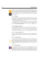
Graphical user interface
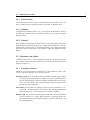
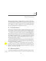
Figure 2.2: Results view. This view is opened at simulation start or upon selection a job
in the job archive (JobQueue). Numbers correspond to sections in the text.
2.2.2
Status and error messages
Status and error messages of simulations executed in local mode are non-intrusively
displayed in the message box below the JobQueue panel. In interactive mode, these
error messages are displayed in a pop-up window.
2.2.3
Job queue and archive
The JobQueue panel provides an overview of pending, running, and completed
simulation jobs and shows the progress and execution time. Jobs can be stopped,
removed and debugged (requires GNU debugger gdb) using the context menu.
Jobs can be grouped and sorted according to model, job ID, state or sweep.
The result browser panel displays the content of the output folder of the currently selected job. The toolbar allows jobs to be stopped (when running) and
to open the output folder in a system-dependent file browser, or a command line
terminal.
2.2.4
2.2.4.1
Simulation output
Visualization
Simulation data can be visualized in various ways. The method of visualization can
be configured in the Analysis element. Gnuplotter is the most versatile tool for
visualization of 2D simulations. It is based on the graphing utility Gnuplot. This
2.2. Simulation and results
9
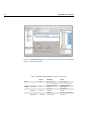
Table 2.1: Output files. Description of common output and result files.
File
logger_[Symbols].log
cells_[Time].png
Description
XML model generated by GUI upon model execution.
Standard output from simulator (as in Output panel).
Error message generated by the simulator.
Compressed XML model with simulation state, created if
and only if checkpointing enabled (Time/SaveInterval).
ASCII text output from the Analysis/Logger plugin.
Plot generated by the Analysis/Gnuplotter plugin.
/jpg/gif/pdf
gnuplot_error.log
Gnuplot error messages (if any).
model.xml
model.xml.out
model.xml.err
[Title][Time].xml.gz
analysis plugin can visualize both cells and PDE layers, provides customizable color
scales, and can display output to screen (wxt, aqua, x11, win) or write to file in a
number of image formats (png, jpg, pdf, svg).
For 3D simulations, the TIFFPlotter provides writing image stacks that may
contain 2D-5D data in the format [X, Y, Z, time, channel] that can be read by
external image analysis software such as Fiji or ImageJ. Alternatively, 3D simulation
data can be written to VTK format using VTKPlotter for post-hoc visualization
with ParaView.
The frequency of visualization is set by the interval attribute of the particular
Analysis element.
2.2.4.2
Logging and analysis
Simulation data can be exported to log files, either as raw data or in processed form.
The Logger plugin writes cell property values or PDE values, optionally reduced
after summing or averaging. The SpaceTimeLogger provides a way to write values
of a linear PDE layer or a slice of a 2D/3D PDE layer to construct space-time
plots. The HistogramLogger constructs and outputs frequency distributions of
cell properties in a population.
The result files are standard tab-delimited text files that can be imported and
processed by external statistical software. Additionally, these logging tools include
a Plot function to visualize the data.
The frequency of data output is set by the interval attribute of the particular
Analysis element.
2.2.4.3
Output folder
Simulation data is written to a folder [Title]_[JobID] within the simulation folder
configured in Settings/Local. Before execution, the model XML file (i.e. model.xml)
and dependent files (e.g. TIFF images) are written/copied to this folder. During
execution, simulation output is written to the same folder. The contents of the
output folder can be browsed by selecting the job in the JobQueue panel. Table
2.1 gives an overview of the files in the output folder.
10
Graphical user interface
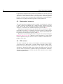
Table 2.2: SBML import. Translation of SBML concepts (red) into Morpheus model
description language (blue).
SBML
Morpheus MDL
Species
Property
Parameter
Property / Constant
InitialAssignment
InitProperty
Inlined in RateRule
Functions
AssignmentRule
Equation
RateRule
DiffEqn
AlgebraicRule
not supported
Reaction
Event
2.2.5
Comment
Units are discarded
Depends on constant attribute
Event
Converted to RateRule
Delays are not supported
Restoring and checkpointing
Models in the job archive can be restored by opening the file: model.xml. This
opens the initial state of the simulation model as a new document.
When using checkpointing (Time/SaveInterval), the complete simulation
state is saved as a compressed XML file ([Title][Time].xml.gz) at the specified
interval. These files can be restored in the same way, however, in this case, a new
document is opened containing the complete simulation state at time [Time].
2.2.6
SBML import
Morpheus supports importing SBML models for intracellular dynamics. SBML
(Systems Biology Markup Language) is a standard for describing models of biochemical pathways. SBML models can be generated using SBML simulators such
as Copasi or downloaded from public repositories such as the BioModels database.
Upon importing an SBML model, the SBML model is converted into systems
of ordinary differential equations for intracellular dynamics in Morpheus model
description language (MDL). Some SBML constructs can be translated in a oneto-one fashion into Morpheus MDL while others require a more elaborate conversion
(see table 2.2).
In general, SBML models are imported in the following way (SBML constructs
in red and Morpheus MDL constructs in blue):
1. A new non-spatial single-cell Morpheus model is created. This model specifies
a single lattice site and a population of 1 cell. A CellType is created to
contain the system of ordinary differential equations.
2. Matching concepts such as Species, Events, InitialAssignments, etc.
are translated from SBML into the Morpheus MDL concepts of Property,
Constants, Events, InitProperty, etc..
3. Reactions in the SBML model are, together with the associated KineticLaws
and Functions, converted into SBML RateRules. These RateRules are
2.3. Parameter sweeps
subsequently assembled into a System of differential equations (DiffEqn)
such that a single differential equation describes the temporal evolution of a
Species or Parameter.
4. Unlike in SBML, the symbolic identifier of a Property or a Constant must
be unique in Morpheus MDL. Therefore, if necessary, Reaction parameters
are renamed upon import by appending the sequential reaction number.
5. Simulation details are not specified in SBML models but are required for
simulation. Therefore, default values are set during the import process. Simulation time is assumed to run from 0...1 by setting Time/StartTime=”0”
and Time/StopTime=”1”. The System solver is set to Runge-Kutta (RK4)
by setting solver =”runge-kutta” and its time-step=”0.01”.
6. Finally, simulation output is preconfigured with a graphical visualization of
the time course data of all species using Analysis/Logger/plot.
Note that not all SBML concepts can be converted into Morpheus MDL. In particular, multiple compartments are not supported, and conversion of delay equations
is not possible (since Morpheus only supports delay differential equations with constant delays, see section 3.2.3). Furthermore, note that units and dimensions are
discarded upon import.
After importing an SBML model into Morpheus, it can be extended into a
spatial, multicellular or multiscale model. Alternatively, it can be copied as a
module into an existing model using the Clipboard (see section 2.1.7).
2.3
Parameter sweeps
The GUI provides a convenient interface for batch processing by generating multiple
jobs with different parameter sets. All parameters (Attributes and Expressions) can
be selected for parameter sweep, using the context menu item ParamSweep. Upon
selection, the parameter appears in the ParamSweep view (fig. 2.3). This is opened
when selecting the ParamSweep element in the Documents panel. This shows the
XML path of the parameter and its type. The range of values for batch processing
can be set be editing the values in the third column. Values can be given explicitly
as semicolon-separated lists or using the list expansion syntax as shown in table
2.3.
2.3.1
Multiple parameters
By default, parameter sets will be combined in a combinatorial fashion, such that a
job is created for each combination of parameter values. Note that the number of
simulation jobs can get prohibitively large for multiple parameters. The number of
jobs is calculated for the current configuration and displayed above the parameters.
To have multiple parameters set simultaneously changing sets, a parameter
can be dragged on another to couple them in a pairwise fashion. Note that these
parameter sets should be of the same length, otherwise, the lowest number of
parameter values is used for the paired set.
11
12
Graphical user interface
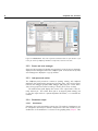
Figure 2.3: Parameter sweep view. This view is opened when selecting the ParamSweep
element in the Documents panel.
Table 2.3: Syntax for list expansion in parameter sweep view.
List
Range
Increment
Intervals
Logarithmic
Syntax
Examples
Result
x;x;x
1.0;1.5;3.0
1.0;1.5;3.0
10 10 10;20 20 20
10 10 10;20 20 20
square;hexagonal
square;hexagonal
0:2:10
0;2;6;8;10
0.5:1:3
0.5;1.5;2.5
0:#2:10
0;5;10
0:#4:1.0
0;0.25;0.5;0.75;1.0
1:#2log:100
1;10;100
x:x:x
x:#x:x
x:#xlog:x
2.3. Parameter sweeps
2.3.2
Simulation and results
Parameter sweeps are executed from the ParamSweep panel using the Start button
in the toolbar. Note that the ParamSweep panel must be opened in order to start
a parameter sweep. Upon execution, a folder [Name of Sweep] is created that
contains a file sweep_summary.txt and subfolders for each simulation job. The
file contains the folder names for the individual jobs and their parameter sets. and
can be used for post-hoc analysis.
2.3.3
Restoring parameter sweeps
Settings of previous parameter sweeps can be restored from the JobQueue provided
that the selected model defined the same parameters and symbols.
13
3
Model formalisms
Morpheus supports the simulation of discrete cellular Potts models as well as continuous ordinary differential equations (ODEs) and reaction-diffusion systems. These
core model formalisms are implemented in a modular way such that they can be
flexibly integrated into multiscale models. Moreover, the modularity enables them
to be combined into auxiliary formalisms such as finite state machines, cellular
automata, coupled ODE lattices or gradient-based models.
3.1
The System construct
The System is a mathematical construct in Morpheus MDL that plays a central
role in modeling of temporal dynamics including ordinary differential equation,
reaction-diffusion systems as well as rule-based models such as cellular automata.
A System is an environment for tightly coupled sets of (differential) equations.
Rules or differential equations in a System environment are updated synchronously
such that the states of variables at time t are calculated on the basis of the state
of the variables at the previous time t − ∆t. Algebraic loops within or between
rules or differential equations are allowed (only) within a System. Therefore, recurrence equations (Rule) or tightly coupled differential equations (DiffEqn) can
be modeled within this environment.
A System is associated with a numerical solver and a time-step (as explained
in section 3.2.1). The time-step sets the integration time step used by the solver
and should be set by the user on the basis of performance (large time-step) and
accuracy (small time-step) considerations.
In addition, the System has an optional attribute time-scaling (default =
1.0) which scales the time within a System relative to the global time. This
automatically scales the System time-step such that the numerical accuracy is
preserved. The time-scaling attribute provides a convenient way to scale the
dynamics of sub-models to each other.
3.2
Differential equations
A number of numerical solvers are available for (a subset of) ordinary, stochastic, delay and partial differential equations to solve initial value problems (Cauchy
15
16
Model formalisms
Table 3.1: Numerical solvers for ordinary and stochastic differential equations.
Method
Numerical scheme
Euler
yn+1 = yn + ∆tf (tn , yn )
Heun (midpoint)
yn+1 = yn + 12 ∆tf (tn , yn ) + f (tn+1 , y˜n+1 )
where
y˜n+1 = yn + ∆tf (tn , yn )
Runge-Kutta (RK4)
yn+1 = yn + 16 ∆t(k1 + 2k2 + 2k3 + k4 )
where
k1 = f (tn , yn ),
k2 = f (tn + 12 ∆t, yn + 12 ∆tk1 ),
k3 = f (tn + 12 ∆t, yn + 12 ∆tk2 ),
k4 = f (tn + ∆t, yn + ∆tk3 )
Euler-Maruyama
yn+1 = yn + ∆tf (tn , yn ) +
Heun-Maruyama
yn+1 = yn + 12 ∆tf (tn , yn ) +
√
∆t∆Wn
q
1
∆t∆Wn + f (tn+1 , y˜n+1 )
2
where
q
y˜n+1 = yn + ∆tf (tn , yn ) + 12 ∆t∆Wn
problems) of the form dy
dt = f (t, y(t)) together with the initial condition y(t0 ) = y0 .
Differential equations (DiffEqn) must be specified inside a System element that
provides an environment for synchronous updating of tightly coupled updated differential equations.
3.2.1
Finite difference solvers
Morpheus implements finite difference methods, Euler, Heun and Runge-Kutta (see
table 3.1). The method to be used for a set of differential equations is specified in
System/solver. All solvers have a fixed time-step that must be specified by the
user in System/time-step.
Note that forward solver methods are not suitable for solving stiff systems
and may require small time-steps to guarantee stability and sufficient accuracy.
All solvers use fixed time stepping; adaptive time stepping solvers are not yet
implemented.
3.2.2
Stochastic differential equations
For stochastic differential equations, the Euler-Maruyama or Heun-Maruyama
method is used (see table 3.1). These methods scale the noise amplitude to the
time-step h that is used. Morpheus automatically switches to Maruyama solvers
3.3. Reaction-diffusion models
when a DiffEqn contains a normally distributed random number, i.e. rand_norm([mean],[stdev]).
Note that other random number distributions, e.g. uniform or gamma distributions, are not allowed in this context. Moreover, stochastic differential equations
cannot be solved using the Runge-Kutta method.
3.2.3
Delay differential equations
Morpheus supports delay differential equations through the use of a property
with a delay, a DelayProperty. This property has an attribute delay that specifies
the length of history, i.e. the lag between assignment of a value and the time at
which it is returned.
Note that only constant time delays are supported. Further note that the delay
must be a multiple of the solver time-step*time-scaling. Also note that a delay
smaller than this time-step has no effect.
3.2.4
Initial condition
Initial conditions for cell-bound variables, i.e. Celltype/Property can be specified
in various ways, depending on whether the initial condition should be specified in a
homogeneous or heterogeneous way or to set an initial conditions in a cell-specific
fashion.
3.2.4.1
Homogeneous population
The value specified in Celltype/Property/value serves as an initial condition
for the whole population of this Celltype. Therefore, this method defines a cell
population that is homogeneous with respect to this variable.
3.2.4.2
Heterogeneous population
A heterogeneous cell population in which initial conditions differ per cell may be
configured using a mathematical expression in Population/InitProperty. This
enables setting initial conditions according to cell ID (cell.id), cell position
(cell.center.x) or using random distributions (e.g. rand_uni([min],[max])).
3.2.4.3
Cell-specific initial conditions
Initial conditions may be specified for each cell separately in Population/Cell/PropertyData, and likewise for vector and delay properties. When using checkpointing, the state of each cell-bound variable is stored here.
3.3
Reaction-diffusion models
Solvers are available for initial boundary value problems on a one-, two- or three∂2y
dimensional domain of length L of the form ∂y
∂t = D ∂x2 + f (t, y(t)) with initial
17
18
Model formalisms
conditions y(t0 , x) = y0 (x) and a set of boundary conditions such as y(t, 0) =
y(t, L) = 0. Reaction-diffusion systems are solved using the sequential operator
splitting method in which the original problem is split into two subproblems (the
reaction and diffusion steps) that are solved sequentially, both for the same timestep. For the reaction step, one of the finite difference methods is used, as described
above (section 3.2).
3.3.1
Diffusion
The diffusion equation is solved using the central difference method. The diffusion coefficient D is specified for each species in the reaction-diffusion systems
in Layer/Diffusion (default: 0.0). The spatial discretization h is specified in
Space/Lattice/NodeLength (default: 1.0).
During initialization, the numerical time-step for the reaction step is adopted
by the diffusion problem. If necessary, the time-step is automatically adjusted in
order to satisfy the Courant–Friedrichs–Lewy (CFL) condition, 2d D ∆t
h2 ≤ 1 where
d = 1, 2, 3 is the number of dimensions.
3.3.2
Boundary conditions
Boundary conditions can be either periodic (default), constant (Dirichlet) or
noflux (Neumann). These are specified in Space/Lattice/BoundaryConditions
for each boundary separately (x, -x, y, -y, z, -z). Note that the type of boundary
condition is shared for all spatial model components (although values may differ).
3.3.2.1
Constant boundary value
In case of constant boundaries, for each species in the reaction-diffusion system,
a value for each boundary should be specified in PDE/Layer/BoundaryValue (default: 0.0).
3.3.2.2
Irregular domains
To solve reaction-diffusion systems in irregular domains, as often required in imagebased systems biology, a shaped domain may be loaded from a TIFF image in
Space/Lattice/Domain/Image. This TIFF must be in 8-bit format in which zero
pixels are interpreted as background (outside domain), non-zero pixels are set
as foreground (inside domain). Irregular domains can have constant or noflux
boundaries.
3.3.3
Initial condition
Initial conditions for each species in the reaction-diffusion system can be set using mathematical expressions in PDE/Layer/Initial/InitPDEExpression. This
enables setting up random initial conditions or spatial gradients. By specifying
symbols for space and lattice size using user-defined symbols (see table 4.1), heterogenous initial conditions can be specified, independent of spatial discretization.
3.4. Cellular Potts model
19
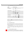
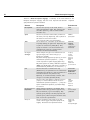
Table 3.2: Cellular Potts model parameters and their location in the model description
language.
Symbol
Description
Metropolis kinetics
T
Y
N
Temperature
Yield
Neighborhood
Sampling / stepper algorithm
Interaction energy
temperature
yield
Neighborhood
stepper
CPM/Interaction
J
Interface energy
Vt
λV
Pt
λP
Target volume
Strength of volume constraint
Target perimeter
Strength of perimeter constraint
µ
Chemotactic sensitivity
Shape constraints
Contact
CellTypes/CellType
Non-Hamiltonian
3.4
Morpheus MDL
CPM/MetropolisKinetics
VolumeConstraint/target
VolumeConstraint/strength
SurfaceConstraint/target
SurfaceConstraint/strength
CellType/CellType
Chemotaxis/strength
Cellular Potts model
The cellular Potts model (CPM) is a cell-based time-discrete method that represents individual cell shapes as lattice domains and models cell motility in terms
of energy minimization using modified Metropolis kinetics. Table 3.2 provides an
overview of how cellular Potts model parameters are encoded in Morpheus MDL.
3.4.1
Modified Metropolis kinetics
A CPM defines cell shape and motility constraints in terms of energetical constraints, described in a Hamiltonian. Motility arises from updating the lattice
configuration according to energy minimization, based on a modified Metropolis
kinetics, with the following steps.
First, a lattice site x (target site) is chosen at random with uniform distribution
(see 3.4.2). Second, a lattice site x0 (trial site) is chosen from the neighborhood
Nx , with uniform distribution (see 3.4.3). Then, the change in free energy ∆H
is calculated for the case if the state σ at the trial site x0 would be copied to the
target site x. Finally, whether or not this transition is accepted depends on ∆H
according to a Boltzmann probability:
(
1
if ∆H + Y < 0
P (σx0 → σx ) =
−(∆H+Y )/T
e
otherwise
Here, T (for ’temperature’) modulates the probability of unfavorable updates
to be accepted, and represents local protrusions/retractions of the cell membrane.
The parameter Y (for ’yield’) accounts for dissipative effects and represents for
example cytoskeletal resistance to membrane fluctuations.
20
Model formalisms
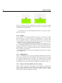
Figure 3.1: Neighborhood Order. Neighborhood of a lattice site (with dot) numbered
according to the minimum neighborhood order in which they are included, for square
(left) and hexagonal (right) lattices.
The parameters for the modified Metropolis kinetics are specified in CPM/MetropolisKinetics.
3.4.2
Stepper
In the standard random stepper algorithm, the target site x is selected at random,
while the trial site x0 is selected from its local neighborhood. In certain cases,
this can be highly inefficient. In sparsely populated lattices, for instance, there
is a high likelihood of selecting sites with identical states that cannot change the
configuration. Selecting such sites is therefore redundant.
To prevent such meaningless updates, Morpheus provides the edgelist stepper. This sampling algorithm tracks all lattice sites that can potentially lead to a
change in configuration and selects the target site x from this list with uniform random distribution. This can yield major improvements in computational efficiency
without affecting model results.
The stepper algorithm can be selected in CPM/MetropolisKinetics/stepper
(default: edgelist).
3.4.3
Neighborhood
The size of the Neighborhood N can be specified using either Distance or Order.
The Distance specifies the maximum Euclidean distance within which lattice sites
are considered neighboring sites. The Order uses a labeling scheme to identify
the neighboring sites. These labels are integer values that alternate between axial
(odd numbers) and radial (even numbers) neighborhoods as shown in figure 3.1.
3.4.4
Monte Carlo Step (MCS) and time scaling
Within the CPM, a Monte Carlo step (MCS) is often interpreted as a discrete unit
of time. A single Monte Carlo step is defined as the number of random sampled
updates equal to the number of lattice sites. That is within one MCS, on average,
each lattice site has been sampled for an update.
3.4. Cellular Potts model
The duration of a single MCS is scaled to the global simulation time as specified
in CPM/MCSDuration (default: 1.0).
3.4.5
3.4.5.1
Cell shape, interaction and motility
Hamiltonian
Each cell occupies a set of lattice sites x with its cell index σ > 0, whereas
σ = 0 refers to the medium. Changes in the spatial configuration of cells on
the lattice are governed by a Hamiltonian H that describes the free energy of
the lattice configuration.
In its simplest form, ignoring intercellular interaction
P
energies, H = σ>0 λV (vσ − Vt )2 where vσ is the actual volume (i.e. number
of lattice sites) of cell σ and Vt is the target volume. Deviations from the target
volume increase the free energy H according to the elasticity parameter λV .
a constraint on the perimeter of the cell is often used, H =
P Additionally,
2
2
λ
(v
−
V
, where pσ is the actual perimeter (i.e.
V
σ
t ) + λP (pσ − Pt )
σ>0
number of interfaces between lattice sites) of cell σ and Pt is the target perimeter
with λP representing the elasticity parameter. The targets and scalars are written
here as constants for simplicity, but can be cell-specific and time-dependent, i.e.
Vt,σ (t), by linking them to cell-bound variables or functions.
Hamiltonian terms for CPM models that constrain cell shape (VolumeConstraint,
ShapeConstraint, LengthConstraint) can be specified in CellTypes/CellType.
3.4.5.2
Interaction energies
The CPM has been originally developed to study the effects of differential adhesion
on cell sorting. Adhesion can be modeled using interaction energies that define a
free energy penalty per interface of contact between cells. Differential cell adhesion
can be modeled by specifying different interaction energies for contacts between
different cells
P σ of different cell types τ . This extends the Hamiltonian with the
term H = interf aces i,j J [τ (σi ), τ (σj )] (1 − δσi σj ) where J is a matrix of interaction energies between different cell types τ (σi ) and σi is the cell at lattice site
i. The Kronecker delta δσi σj = {1, σi = σj ; 0, σi 6= σj } ensures only interfaces
between cells are taken into account.
The matrix of interaction energies between cell types can be specified in CPM/Interaction. These energies are normalized by the number of neighbors such
that the interaction energies are automatically rescaled when the lattice structure
is changed.
Interaction energies can be altered based on the state of a cell property that
represents e.g. cadherin expression (AddonAdhesion) or on the combination of
properties between neighboring cells to represent binding between heterophilic
(HeterophilicAdhesion) or homophilic adhesion molecules (HomophilicAdhesion).
These plugins can be specified in CPM/Interaction/Contact.
21
22
Model formalisms
3.4.5.3
Kinetic terms
The classical CPM has been extended by non-Hamiltonian terms. Since these terms
directly affect the change in energy ∆H and may change the energy of the system,
they are called kinetic terms. A widely used kinetic term biases motility of a cell σ in
the direction of a local concentration gradient of a species wP
in a reaction-diffusion
model in order to represent chemotactic migration: ∆H = σ>0 µ(wx0 − wx ).
Kinetic terms that bias motility (Chemotaxis, Haptotaxis, DirectedMotion,
Persistence) can be specified in CellTypes/CellType.
3.4.5.4
Event-based terms
Other CPM extensions are based on the cell state at the end of a Monte Carlo step
and are evaluated only once per Monte Carlo step, instead of every update trial.
This includes extensions that model cell division (Proliferation) and cell death
(Apoptosis). Proliferation triggers the division of a cell into two daughter
cells, based on a condition. Apoptosis triggers the immediate removal of a cell
(lysis) or setting its target volume to zero (shrinking) and removing the cell
from the population only after it does not occupy any lattice sites.
3.4.5.5
Update-preventing terms
Some CPM extensions act to prevent updates altogether, based on some criterion.
These include the Freezer that disables all updates for a particular cell, based
on a user-specified condition. It also includes the ConnectivityConstraint that
ensures the cell is simply connected by preventing updates that would break this
topological constraint.
3.4.6
Initial condition of spatial configuration
Simulations of cellular Potts models require the specification of at least one population of cells in CellPopulations/Population. By default, the specified number
of cells is distributed randomly in space using a uniform distribution, each cell
occupying a single lattice site.
Spatially structured initial populations can be configured using InitRectangle
and InitCircle. These initializers attempt to fit the specified number of cells in
a regular fashion, with each cell occupying a single lattice site. Note that artefacts
may occur due to spatial discretization.
Initializing a population of cells with geometrical shapes can be configured using
the CellObjects initializer. This allows for the specification of spheres, cylinders,
boxes and ellipsoids that can be arranged along the orthogonal axes.
Cell populations can also be initialized from images using the TIFFReader
initializer. This provides an interface to configure models from microscopy images.
TIFF images may be in 8-, 16-, and 32-bit format and may contain multiple z-slices
(image stacks). By convention, all pixels sharing a particular integer value will be
added to the same cell. The option keep_id ensures that this value is used as a
cell ID internally.
3.5. Auxiliary model formalisms
3.5
Auxiliary model formalisms
The modular design of the formalisms allows a number of auxiliary formalisms to
be constructed. For instance:
Coupled ODE Lattice Coupled ordinary differential equation lattice models can
be used to represent a regularly structured tissue in which each cell is represented by an intracellular ODE model and communicates with its neighboring
cells.
Coupled ODE lattice models can be constructed by configuring a lattice of
cells, each occupying a single lattice site using InitRectangle. A CellType
with a System of DiffEqn describing the intracellular dynamics. Intercellular communication is modeled using a NeighborReporter that reports the
(weighted) average of the properties of directly adjacent neighbor cells.
Cellular Automata (CA) Cellular automata are a widely used discrete-time, discretespace, discrete-variable formalism to study the emergence of macroscopic
behavior from microscopic local rules.
CA models can be constructed by configuring a lattice of cells, each occupying a single lattice site using InitRectangle. A CellType with a System
of synchronously updated Rules describes the state transitions, based on the
states of cells in the local neighborhood, reported using a NeighborReporter.
Gradient based models Gradient-based models can be used to describe patterning of tissues under influence of a morphogen gradient, such as Wolpert’s
classical French flag model.
Gradient-based models are built using a non-diffusive PDE Layer, initialized
by a mathematical expression using an InitPDEExpression. A regular lattice of cells is configured by an InitRectangle, in which each cell measures
the morphogen concentration at its location using a PDEReporter, based on
which an Equation defines the cellular identity.
23
4
Model description language
Morpheus simulation models are specified in a custom domain-specific model description language (MDL). The XML-based language uses biological and mathematical terminology to declaratively describe multiscale multicellular simulation
models. It is composed of human-readable tags to represent the components of
biological processes (table 4.2) and a number of mathematical constructs to define
their dynamics and relations (table 4.3).
Morpheus simulation models are fully specified by single model description
files. These include the definition, configuration and and parameterization of
(sub)models as well as the specification how these (sub)models are interlinked.
Details on the numerical simulations are also stored in the model description file
such as the simulation time, spatial discretization, initial conditions and the configuration of visualization and data output. For checkpointing, the complete state
of a simulation during execution can be stored in the same file format. The fact
that the complete simulation model, including the description of its dynamics, is
encapsulated in single files, render them suitable for archiving as well as model
exchange between users.
4.1
Declarative
The Morpheus model description language (MDL) separates modeling from implementation by allowing the description of models in a declarative fashion. Models
describe what processes are to be simulated rather than how this should be accomplished. This distinguishes declarative languages such as the Morpheus MDL
from imperative programming language such as C++ or Python that focus on the
description of algorithmic control flow.
4.2
Domain-specific
The MDL uses a domain-specific markup language using vocabulary that is derived
from the application domain of multiscale and multicellular systems biology. On
the one hand, it uses concepts such as cell types and populations, and biological
processes such as proliferation and chemotaxis (table 4.2). On the other hand, it
defines a range of mathematical constructs such as constants, functions, equations
25
26
Model description language
and systems of differential equations (table 4.3). This combination of biological
and mathematical terms provides a powerful way to describe the relations and
dynamics of biological processes.
4.3
Encapsulation
Models in Morpheus MDL describe both the model itself and specify details of
its simulation including initial conditions (see table 4.2). During a simulation, the
full simulation state, including the position and state of all cells, can be written
in the same description language. In this way, a single model file contains the full
specification of the model simulation. The encapsulation in a single file significantly
simplifies archiving, checkpointing and restoring simulation models as well as the
exchange of models between users.
4.4
Two-tiered architecture
Morpheus MDL has a two-tier architecture (see figure 4.1). On the one hand, the
XML is used to store information about the model components or sub-models in a
hierarchically structured way. On the other hand, symbolic interdependencies represent the interactions and feedbacks between model components or sub-models.
This combination provides a convenient way to express models of complex biological processes and allows automation of model integration (see chapter 5).
4.4.1
XML
The model description language is based on the eXtensible Markup Language
(XML). This has a number of advantages: It stores information in a well-structured
fashion that can be easily parsed and validated and it allows human-readable
domain-specific terminology and can be extended in a straightforward fashion.
The main elements of the XML structure, as shown in table 4.2, are used to
describe both the structure and parameterization of the model, and the details of its
numerical simulation. The spatio-temporal aspects of the simulation are specified
in the required Space and Time elements, the initial conditions or simulation state
are described in CellPopulations, data output and visualization is configured in
Analysis. The title and annotation of a model are added in the Description
element.
The model itself is configured using the CellTypes, CPM, and PDE elements.
The properties, behavior and dynamics of cells, including intracellular dynamics,
are specified in the CellTypes element. The parameters of the cellular Potts model
are configured in the CPM element and the reaction-diffusion models are defined
and configured in the PDE element. These elements are all optional such that the
various model formalisms can be used in isolation as well as in combination.
The XML represents this information in a hierarchical tree-like structure that
reflects the structure of the modeled biological system. For instance, the main element CellPopulations can contain a Population that contains multiple Cells.
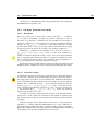
4.4. Two-tiered architecture
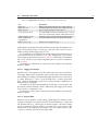
Figure 4.1: Schematic representation of the two-tier architecture. The hierarchical XML
tree provides information on the structure of the model and its components (colored
boxes). By defining and referring to symbolic identifiers, model components can be linked
together in a network (arrows). Systems (rounded grey boxes) provide an environment
for tightly-coupled differential equations in which self-references and circular dependencies
between symbols are allowed.
Similarly, intracellular dynamics are modeled using a Systems of DiffEqn within
a CellType, while the PDE describing extracellular dynamics is defined in its own
element outside of CellTypes.
The XML structure is convenient to represent the hierarchy between the components of a model. However, it is not suitable to describe the network of interactions
and feedbacks between these components, which is done using symbolic identifiers.
4.4.2
Symbols
Model components can be linked using symbolic identifiers. Symbolic identifiers
and references establish interactions and feedbacks between (sub)models to represent the network-like complexity in biological processes (see fig. 4.1).
Symbolic identifiers, or symbols, can be specified to represent user-defined
model variables such as cell-bound properties (Property) or concentrations of
species in a reaction-diffusion model (Layer) (see table 4.1). Symbols can also
27
28
Model description language
be specified for simulation-related constants and variables such as lattice size and
current time of simulation (see table 4.1). Symbols can be used in mathematical
expressions to define relations between model components. Additionally, symbols
provide a convenient way to integrate different (sub)models by defining symbolic
identifiers in one (sub)model and using them in another (sub)model.
4.5
Mathematical constructs
The model description language provides a number of mathematical constructs
to define constants and variables and to express functions, equations and conditional events as well as the specification of tightly coupled systems of differential
equations. An overview of the available constructs is given in table 4.3.
Mathematical expressions may be specified in terms of user-defined or predefined symbols (see table 4.1). Expressions are entered in plain text using standard
infix notation. An overview of the available operators, functions and random number generators and their syntax is given in table 4.4.
Expressions are parsed during initialization using the fast math parser muparser
(muparser.beltoforion.de). Muparser converts expressions to reverse Polish
notation represented in byte code that is used to evaluate the mathematical expressions at run time.
4.6
XML schema
The rules, constraints and contents of the Morpheus model description language
are laid down in an XML schema. The XML schema description (XSD) is embedded in the GUI and provides the information to edit, validate and repair model
descriptions. Although the XML schema validates the XML structure, the GUI
does not check the correctness of symbolic linking and mathematical expressions.
Therefore, syntactically correct models may still result in simulation errors despite
validation by XML schema.
4.6. XML schema
29
Table 4.1: User-defined and pre-defined symbols in Morpheus model description language.
Context
Space
Time
Various
Celltype
CPM
PDE
cell
vectors
Element
Type
Description
Simulation symbols
Lattice/Size
vector
Size of lattice
SpaceSymbol
vector
Current location
NodeLength
double Spatial discretization
StartTime
double Initial simulation time
StopTime
double Termination time of simulation
SaveInterval
double Interval between checkpointing
TimeSymbol
double Current time
Model symbols
Global
double Constant with global scope
Constant
double Constant with local scope
ConstantVector
vector
Constant vector with local scope
Function
double Mathematical expression
Property
double Cell-bound variable
PropertyVector
vector
Cell-bound variable vector
DelayProperty
double Cell-bound variable with delay
MCSDuration
double Time of single Monte Carlo step
Layer
double Reaction-diffusion species
Predefined symbols
cell.id
integer Unique cell index
cell.type
integer Cell type index
cell.volume
integer Number of lattice sites cell occupies
cell.surface
integer Number of lattice sites of cell boundary
cell.center
vector
Center of mass of cell
cell.length
double Cell length of major axis
cell.orientation
vector
Orientation of major axis
[symbol].x/y/z
double Cartesian vector coordinates
[symbol].abs
double Magnitude of vector
[symbol].phi/theta
double Polar coordinates of vector
30
Model description language
Table 4.2: Model description language. A summary of the main elements of the
Morpheus description language and their most important sub-elements. Required
(sub)elements are printed in boldface.
Element
Description
Sub-elements
Description
Sets the name (Title) of the model, used for
naming the destination folder. May include model
annotation (Details), used for human-readable
annotation only.
Sets the size, structure and boundary conditions of
the lattice (Lattice). Optionally, sets a symbols for
the lattice size and current location
(Lattice/Size/symbol and SpaceSymbol).
Set the duration of a simulation (StartTime and
StopTime) defining the global time. Optionally, sets
a symbol for current time (TimeSymbol). May
specify the interval to save the simulation state
(SaveInterval). May set a random seed for
stochastic simulations (RandomSeed).
Allows multiple cell types to be defined. Each cell
type (CellType) sets a name and type (i.e.
biological or medium).
May define multiple properties (Property) for use in
mathematical expressions (Equation, ...). May
contain reporters for spatial mapping (Reporter).
May define systems of ordinary differential equations
(ODE) (System/DiffEqn). May specify a diversity of
cellular behaviors (Chemotaxis, Proliferation, ...).
Sets the time-scale of a Monte Carlo step
(MCSDuration), the parameters for the cellular Potts
model (MetropolisKinetics) and the parameters of
interactions between cells (Interaction).
Optionally, for constant boundary condition, sets a
cell type at a boundary (BoundaryValue).
Sets the symbol and diffusion coeffients for species
(Layer) in a reaction-diffusion model for use in
mathematical expressions (Equation, ...). May set a
system of differential equations (System/DiffEqn)
for reactions.
Allows multiple populations to be defined. Each
population sets a cell type and size (Population).
May set initializers (e.g. Initrectangle). May
explicitly specify multiple cells with properties and
positions (Cell). When saving the simulation state,
state of each cell is specified here.
Sets the visualization and analysis tools. May
contain various loggers and plotters (Gnuplotter,
Logger). Executed at user-specified intervals.
Title
Space
Time
CellTypes
CellType
CPM
PDE
CellPopulations
Population
Analysis
Details
Lattice
SpaceSymbol
StartTime
StopTime
TimeSymbol
SaveInterval
RandomSeed
Property
System
Constant
Function
Equation
Event
Reporter
Chemotaxis
Proliferation
...
Interaction
MetropolisKin.
MCSDuration
BoundaryValue
Layer
Constant
System
Function
Equation
Cell
Initrectangle
TIFFReader
...
Gnuplotter
TIFFPlotter
Logger
HistogramLogger
4.6. XML schema
31
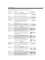
Table 4.3: Mathematical constructs. Overview of the mathematical constructs available
in model description language (• = symbol definition, ◦ = symbol reference).
Element
Description
Symbol graph
Containers
Constant
Constant value of type double with local scope, i.e. valid
within the CellType or System it is defined in.
Global
Constant
Variable value of type double with global scope.
Global
Property
PropertyVector
DelayProperty
Cell-bound variable. Property and DelayProperty are of
type double. DelayProperty has attribute delay to set
the lag between assignment and return of value.
Property
PropertyVector defines Euclidean vector in space
delimited format “x y z”.
Layer
PDE model variable, i.e. species in reaction-diffusion
system. Diffusivity of a Layer is specified in attribute
Layer
diffusion.
Expressions
Function
Equation
Rule
Mathematical expression. Computes a value (double) for
the output symbol it defines, but does not assign it to a
variable. Updated whenever when output symbol is
referenced. May not contain algebraic loop.
Function
Mathematical expression. Computes a value (double) and
assigns it to the variable it references. Updates are
scheduled depending on its symbol dependencies. May
not contain algebraic loop.
Equation
Mathematical expression that defines a (recurrence)
equation for use in environments such as System and
Event. Scheduled according to System/time-step. May
Rule
contain algebraic loop and self-references.
DiffEqn
Mathematical expression that defines a differential
equation. Only allowed in System environment. May
DiffEqn
contain algebraic loop and self-references.
Reporters
Reporter
NeighborsReporter
PDEReporter
...
Explicit data mappings. Computes a statistic (average,
mean, etc.) of the input data and assigns this to the
output symbol. Updates are scheduled depending on its
symbol dependencies.
Reporter
Environments
System
Event
Environment for tightly coupled sets of differential
equations and rules that are synchronously updated (see
section 3.1). Scheduled according to user-specified
System time-step and time-scaling.
Environment for conditional or timed events. Triggered
periodically or, if Condition is specified, whenever the
condition changes from false to true. Updates are
scheduled according to time-step if specified or
depending on its symbol dependencies otherwise.
System
Event
32
Model description language
Table 4.4: Operators and predefined functions available in mathematical expressions.
Class
Description
Syntax
Operators
Addition
Subtraction
Multiplication
Division
Power
Logical and
Logical or
Exclusive or
Equal
Not equal
Smaller
Greater
Smaller or equal
Greater or equal
Sine
Cosine
Tangens
Arc sine
Arc cosine
Arc tangens
Hyperbolic sine
Hyperbolic cosine
Hyperbolic tangens
Arc hyperbolic sine
Arc hyperbolic cosine
Arc hyperbolic tangens
Logarithm base 2
Logarithm base 10
Natural logarithm
Exponent
Power
Square root
Sign, -1 if x<0, 1 if x>0
Round nearest integer
Absolute
Minimum of arguments
Maximum of arguments
Sum of arguments
Average of arguments
Modulus, remainder
Uniform distribution
Normal distribution
Gamma distribution
Boolean (0 or 1)
Conditional statement
+
Logical operators
Comparison
Functions
Random number
Condition
*
/
^
and
or
xor
==
!=
< or &lt;
> or &gt;
<= or &lt;=
>= or &gt;=
sin(...)
cos(...)
tan(...)
asin(...)
acos(...)
atan(...)
sinh(...)
cosh(...)
tanh(...)
asinh(...)
acosh(...)
atanh(...)
log2(...)
log(...)
ln(...)
exp(...)
pow([base], [exponent])
sqrt(...)
sign(...)
rint(...)
abs(...)
min(..., ..., ...)
max(..., ..., ...)
sum(..., ..., ...)
avg(..., ..., ...)
mod([numer], [denom])
rand_uni([min], [max])
rand_norm([mean], [stdev])
rand_gamma([shape], [scale])
rand_bool()
if([condition], [then], [else])
5
Model integration
Morpheus supports the integration of time-discrete cell-based models with timecontinuous models for intra- and extracellular dynamics. In particular, cellular Potts
models (CPM) can be linked to ordinary, stochastic or delay differential equations
as well as to reaction-diffusion (PDE) models. The Morpheus model description
language facilitates the specification of links between (sub)models with the help of
symbolic identifiers (see chapter 4).
For the user, a link between sub-models is established by simply defining a
symbol in one sub-model and using it as an input in another sub-model, providing
a convenient way to construct and explore complex multiscale biological systems
using integrative models. During simulation, Morpheus makes the data accessible
between sub-models and, if necessary, mapping or transforming it to make it suitable for the target sub-model. Moreover, the updates of the various sub-models are
appropriately scheduled, by determining the correct order and the frequency of updates, as to guarantee that up-to-date data is used in all computations. Both tasks
are handled automatically as far as possible, based on user-specified time-steps and
symbolic interdependencies.
5.1
Spatial mapping
Integration of spatial model formalisms, i.e. cell-based and reaction-diffusion models, requires that the data from one sub-model is accessible to the other sub-model.
In Morpheus, data is not copied between sub-models, but is directly accessible
through symbolic identifiers. Yet, the data must be accessed in a way that is
appropriate for the model that uses the symbol. The model that uses a symbol
determines the lattice sites for which the symbol is resolved, whereas the model
that defined it determines the value of the symbol at those lattice sites.
Morpheus uses the convention that the spatial discretization in cell-based and
reaction-diffusion models is identical. The lattice size (Lattice/Size) and the
physical interpretation of the size of a lattice site (Lattice/NodeLength) are
shared by both CPM and PDE models, which simplifies their integration. Therefore, in some cases, the mapping is trivial enough to be handled automatically.
In other cases, a more complex mapping is required such as calculating a sum or
average which requires the explicit instructions by the user using a Reporter.
33
34
Model integration
5.1.1
Automated mapping
Mappings that present an unambiguous relationship are resolved automatically.
For instance, when non-spatial constants and variables are used within a spatial
context, the same value is used for all lattice sites over which is iterated. The use
of symbols referring to cell-boundary Properties within reaction-diffusion (PDE)
models linking PDE to CPM models can also be handled automatically. In that case,
for each lattice site for which the PDE Layer is defined, the value of the cell
property of the cell at that site is used.
The reverse case, when PDE variables are used in CPM models, can be automatically mapped, only in certain cases. For instance, in the Chemotaxis extension,
cell motility is biased by the gradient of concentration of a species in a reactiondiffusion model. Here, the difference in concentrations of the PDE variable at the
target and trial site is automatically resolved (see 3.4.5.3).
5.1.2
Explicit mapping with Reporters
When the mapping between the two contexts is not unambiguous, a statistic is
required to define how a symbol should be mapped. This requires the user to
specify an appropriate way to transform the data from one (sub)model to the
other (sub)model. Defining such an explicit mapping is done using a Reporter.
The NeighborsReporter calculates the (weighted) average or sum of the cellbound Property in adjacent cells given by the input symbol and assigns this
statistic to its output symbol.
The PDEReporter maps PDE variables for use in cell-based models by reporting
the average, sum, maximum or gradient of concentration of the input PDE/Layer
at the lattice sites occupied by the cell or, optionally, its discretized center of mass.
5.2
Scheduling
Integration of time-continuous ODE and PDE models with time-discrete CPM
models and various auxiliary mathematical constructs requires a careful scheduling of numerical updates. While the general simulation schedule is executed in
fixed order, some processes must be scheduled according to the symbolic interdependencies in order to guarantee correctness of simulation results. The simulation schedule is computed during intializatoin and printed to the standard output
(model.xml.out).
5.2.1
Simulation schedule
The general simulation cycle follows a fixed order in which temporal models are
executed before the sequential processes and output processes, as shown in figure
5.1. The scheduling of sequential processes such as Reporters and Equations
involves the determination of the order of updates as well as the setting of intervals
in which the various model components should be computed.
5.2. Scheduling
35
Initialization
Simulation cycle
1
Lattices
Termination
Analysis
CPM
Cell types
Save state
CPM
Systems
Diffusion
PDE
x
Reporters
2
Equations
Reporters
Events
Equations
3
Analysis
StopTime
Symbols
StartTime
Cell populations
Analysis
Save state
Save state
Figure 5.1: Overview of the general simulation schedule. Between initialization and
termination, the simulation cycle is iteratively executed until time=StopTime. A single
simulation cycle proceeds in three phases. First, the temporal models such as CPM ,
Systems and Diffusion are updated according to user-defined time-steps. Second, the
sequential processes such as Equations and Reporters are updated in an order and
interval that is determined by dependencies between symbols. Third, output is generated
and the simulation state is written to file at user-defined intervals.
Initialization
First, the lattice is created and initialized, cell types are created, the CPM is initialized, and PDE layers are created and initialized (PDEInitExpression). Afterwards,
populations of cells are created and put in the lattice randomly or according to a
user-specified initializer (e.g. InitRectangle). Then, symbols are registered and
set to initial values. Afterwards, Reporters and Equations are run once to initialize
all remaining symbols. Finally, the analysis and visualization tools (Analysis) are
run, and the simulation state is saved to file.
Simulation cycle
The simulation cycle is iterated from StartTime to StopTime in steps that advance
according to the smallest time step (section 5.2.3). In each iteration, the processes
that are scheduled for the current time step are executed in the following order.
1. Temporal models: The time-dependent models are executed. A single
Monte Carlo Step is performed for the CPM. Afterwards, Systems and Diffusion
are updated.
36
Model integration
2. Sequential processes: Non-time-dependent models such as Equations,
Reporters and Events are updated. Their order is computed from their
symbolic interdependencies (section 5.2.2).
3. Analysis: Finally, visualization and data output is updated and the simulation state is saved to file.
Termination
At the end of simulation, visualization and analysis tools specified in Analysis tools
can be executed once more and the simulation state is written to file.
5.2.2
Scheduling update order
The order of execution is independent of the order in which model components
are specified in the model description file. Rather, updates of temporal processes
(CPM, System, Diffusion) are scheduled according to the fixed schedule shown in
figure 5.1 and updates of sequential processes such as Equations and Reporters
are scheduled according to their symbolic interdependencies.
Sequential processes are ordered according to the dependencies in their input
and output symbol based on the following rule:
• Before updating a process, its input symbols must all be updated.
This is achieved by scheduling all processes that have these symbols as an output
before. Note that this is only possible if no algebraic loops or circular dependencies
exist between these processes. Therefore, such loops are only allowed within the
System environment.
The order of execution of data output and visualization in Analysis is arbitrary
and does not affect the simulation itself. Therefore, these are executed in the order
in which they are given in the model description file.
5.2.3
Update interval
The simulation cycle is iterated for the period from StartTime to StopTime, called
the global simulation time. The number of iterations that are executed during this
period depends on the temporal process with the smallest time step. During each
iteration, only the processes that require updating are executed. The intervals at
which each process requires updating are determined during initialization, based
on user-specified time-steps or symbolic interdependencies.
The frequency in which CPM and Systems are updated is based on user-specified
information. The update interval of CPM models is the duration of a single Monte
Carlo step, specified in CPM/MCSDuration (see 3.4.4). The update interval of
a System is determined by its time-step, divided by time-scaling (see 3.1).
Similarly, the intervals at which Analysis processes are executed to do visualization
and data analysis also depend on a user-specified interval.
5.2. Scheduling
The update intervals of other processes such as Equations, Reporters, Events
and Diffusion are automatically determined by propagation of the intervals of
their input and output symbols, according to the following rules:
• The process is updated as often as its output symbol(s) are used.
• The process is not updated more often than its input symbol(s) can change.
The former ensures that up-to-date data is used in all processes, while the latter
improves computational performance by preventing redundant computations. Note
that processes are not scheduled and computed if their output symbol(s) is (are)
not used.
The interval of Diffusion is likewise determined by the interval of its output
symbol, but it may iterate multiple times with smaller intervals as to satisfy the
CFL stability criterion (see 3.3.1). Functions are not explicitly scheduled and
do not have an update interval. Instead, they are updated whenever their output
symbol is used, but at most once per minimal time step. User-specified intervals
for Analysis processes smaller than the minimal time step are ignored, since the
state of the simulation cannot change within this interval.
The final simulation schedule including the computed order of execution and
update intervals is calculated at the end of initialization and printed to the standard
output. This is written to the output file model.xml.out and is displayed in the
output text box of results view in the GUI (see 2.2).
37
Table 5.1: Example models are available in the application and described on the website.