Download DAGitty User Manual

DAGitty User Manual
Johannes Textor
October 13, 2010
Abstract
DAGitty is a program for creating, editing, and analyzing causal models, known in epidemiology as directed acyclic graphs (DAGs). The main task of the program is to assist the
user in identifying adjustment sets – that is, sets of covariates to adjust for in order to isolate
the causal effects from an exposure to an outcome from the non-causal (or confounded) effects.
DAGitty runs in any web browser that supports modern HTML and JavaScript.
Contents
1 Introduction
1.1 Causal models . . . . . . . . . . . . . . . . . . . . . . . . . . . . . . . . . . . . . .
1.2 Running DAGitty online . . . . . . . . . . . . . . . . . . . . . . . . . . . . . . . .
1.3 Installing DAGitty on your own computer . . . . . . . . . . . . . . . . . . . . . . .
2
2
2
3
2 Loading and saving models
2.1 DAGitty’s textual syntax for causal models
2.2 Loading a model into DAGitty . . . . . . .
2.3 Modifying the graphical layout of a model .
2.4 Saving the model . . . . . . . . . . . . . . .
3 Editing models within DAGitty
3.1 Adding new variables . . . . . . . .
3.2 Adding new connections . . . . . .
3.3 Deleting variables . . . . . . . . . .
3.4 Deleting connections . . . . . . . .
3.5 Setting exposition and outcome . .
3.6 Workarounds for functions that are
.
.
.
.
.
.
.
.
.
.
.
.
.
.
.
.
.
.
.
.
.
.
.
.
.
.
.
.
.
.
.
.
.
.
.
.
.
.
.
.
.
.
.
.
.
.
.
.
.
.
.
.
.
.
.
.
.
.
.
.
.
.
.
.
.
.
.
.
.
.
.
.
.
.
.
.
.
.
.
.
.
.
.
.
3
3
3
3
4
. . . . . . .
. . . . . . .
. . . . . . .
. . . . . . .
. . . . . . .
still missing
.
.
.
.
.
.
.
.
.
.
.
.
.
.
.
.
.
.
.
.
.
.
.
.
.
.
.
.
.
.
.
.
.
.
.
.
.
.
.
.
.
.
.
.
.
.
.
.
.
.
.
.
.
.
.
.
.
.
.
.
.
.
.
.
.
.
.
.
.
.
.
.
.
.
.
.
.
.
.
.
.
.
.
.
.
.
.
.
.
.
.
.
.
.
.
.
.
.
.
.
.
.
.
.
.
.
.
.
.
.
.
.
.
.
.
.
.
.
.
.
4
4
4
4
5
5
5
. . . . .
. . . . .
models .
. . . . .
.
.
.
.
.
.
.
.
.
.
.
.
.
.
.
.
.
.
.
.
.
.
.
.
.
.
.
.
.
.
.
.
.
.
.
.
.
.
.
.
.
.
.
.
.
.
.
.
.
.
.
.
.
.
.
.
.
.
.
.
.
.
.
.
.
.
.
.
5
5
6
6
6
4 Adjustment sets
4.1 Minimal sufficient adjustment sets . . . . .
4.2 Finding minimal sufficient adjustment sets .
4.3 Verfiying that all paths are blocked in small
4.4 Adjusting for specific covariates . . . . . . .
.
.
.
.
5 Acknowledgements
6
6 Legal notice
7
7 Bundled libraries
7
8 Bundled examples
7
9 Author contact
7
1
1
1.1
Introduction
Causal models
To convey an idea of the purpose of DAGitty, this introduction contains some very small examples
of causal models, confounding and adjustment sets; for a more detailed discussion of these subjects,
we recommend the book Causality by Judea Pearl [6].
Causal models are also called Bayesian networks (in computer science) or even DAGs (in
epidemiology).1 Simply put, a DAG is a formal model about causal relationships between certain
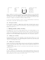
entities of interest in a specific scenario. For example, the sentence “smoking causes cancer” could
be translated into the following simple causal model:
smoking
cancer
Figure 1: A very simple causal model.
An important application for causal models, which is also the focus of DAGitty, is to isolate
the causal effects of a variable of interest, called exposure onto another, called outcome, from the
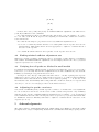
confounded relations between the two variables. For example, consider the following, slightly more
complex causal model:
smoking
?
carry matches
cancer
Figure 2: A classical confounding triangle.
If we were to perform a study on the relationship between carrying matches in one’s pocket
and developing lung cancer, we would probably find a correlation between these two variables.
However, as the above model indicates, this correlation would not imply that carrying matches in
your pocket causes lung cancer: Smokers are more likely to carry matches in their pockets, and
also more likely to develop lung cancer. This is a classical example of a confounded association
between two variables. In this example, would we control for smoking, i.e. put smokers and nonsmokers in two different groups, we would probably no longer find a correlation between carrying
matches and lung cancer.
In general, any set of variables in a causal model that blocks all confounded (i.e., non-causal)
effects between an exposition and an outcome, but does not affect the causal effects, is called
a sufficient adjustment set. If the causal model is accurate, then adjustment, stratification, or
selection (e.g. by restriction or matching) for this set of variables in an epidemiological study will
minimize bias when estimating the effect of exposition on outcome in an epidemiological study.
Adjustment sets will be explained in more detail in Section 4.
The purpose of DAGitty is to aid epidemiological study design through the identification of
suitable, small sufficient adjustment sets in complex causal models.
There are two ways to run DAGitty: either from the internet or from your own computer.
1.2
Running DAGitty online
To run DAGitty online, simply open its URL in your favourite Browser:
1 Calling bayesian networks “DAGs” is of course highly confusing to computer scientists and mathematicians,
for whom a DAG is simply an abstract graph without specific semantics attached to it.
2
http://www.tcs.uni-luebeck.de/software/dagitty/
DAGitty should run in every modern Browser. If it doesn’t, please send me an E-Mail so I
can fix the problem; see contact information at the end of this manual.
1.3
Installing DAGitty on your own computer
DAGitty can be “installed” on your computer for use without an internet connection. To do this,
download the file
http://www.tcs.uni-luebeck.de/software/dagitty/dagitty.zip
which is a ZIP archive containing DAGitty’s source. Unpack this ZIP file anywhere on your
local hard drive. To run DAGitty, just open the file dags.html in the unpacked folder.
2
Loading and saving models
This section covers the three basic steps of working with DAGitty: (1) Loading a model; (2)
manipulating the graphical layout of the model; and (3) saving the model. First of all, any causal
model consists of vertices (variables) and edges (relationships between variables). You can either
R and then import this description
create the model in a text editor such as Microsoft Word into DAGitty, or create the model in DAGitty itself using the graphical user interface (see next
section). In addition, DAGitty contains some pre-defined examples that you can use to become
familiar with the program. To do so, select one of the pre-define examples from the drop-down
menu below the legend and click on “draw DAG”.
2.1
DAGitty’s textual syntax for causal models
DAGitty’s textual syntax for causal models is compatible with the one used by the DAG program
by Sven Kn¨
uppel [4]. A model description consists of two parts:
1. A list of the variables in the model
2. A list of connections between the variables
The list of variables is simply one variable per line (blank lines are ignored by DAGitty). By
convention, the variable in the first line is the exposure and the variable in the second line is the
outcome of your model. Variable names must not contain spaces or colons; please use dashes or
underscores instead (i.e., write fitness_level instead of fitness level).
The list of connection consists of several lines each starting with a start variable name, followed
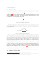
by one or more other target variables that the start variable is connected to. Figure 3 contains a
working example of a textual model description. When you modify a model within DAGitty, the
vertex labels will be augmented by additional information, to help DAGitty remember the layout
of the vertices and for other purposes (see rightmost column in Figure 3).
2.2
Loading a model into DAGitty
To load a textually defined model into DAGitty, simply copy&paste the variable list into the
“vertex labels” text field and the list of connections into the “adjacency list”. Then click on “draw
DAG”. DAGitty will now generate a preliminary graphical layout for your model on the canvas,
which may or may not be aesthetically pleasing, but can be freely modified.
2.3
Modifying the graphical layout of a model
To layout the vertices and edges of your model more clearly than DAGitty did, simply drag the
vertices with your mouse on the canvas. You will notice that DAGitty modifies the list of vertices
in the “vertex labels” text field on the fly, and augments it with additional position information
3
vertex labels
E
D
A
B
Z
adjacency list
ED
AEZ
BDZ
ZED
resulting graph
A
B
Z
E
augmented vertex labels
E 1 @-2.2,1.6
D 1 @1.4,1.6
A 1 @-2.2,-1.5
B 1 @1.4,-1.5
Z 1 @-0.3,-0.1
D
Figure 3: Example for a textual model definition with DAGitty. When the model is edited within
DAGitty, the vertex labels are augmented with additional information that DAGitty uses to
layout the vertices on the canvas (rightmost column): In the second column, weights are given for
each variable (not used yet, but perhaps in future versions of DAGitty) and in the third column,
the layout coordinates of each variable are indicated behind the @ sign.
for each vertex. In general, all changes you make to your model within DAGitty are immediately
reflected in the “vertex labels” and “adjacency list” text fields.
2.4
Saving the model
To save your model locally, just copy&paste the contents of the “vertex labels” and “adjacency
R document, and save that file locally to
list” text fields to a text file, e.g. a Microsoft Word your computer. Next time you wish to work on the model, copy the model description back into
DAGitty as explained above.
3
Editing models within DAGitty
As explained above, you are free to make changes directly to the textual description of your
model, which will be reflected on the canvas next time you click on “draw DAG”. However, you
can also create, modify, and delete vertices and connections on the canvas itself. All such changes
to the model are immediately reflected in the “vertex labels” and “adjacency list” text fields.
Furthermore, the list of minimal sufficient adjustment sets (see next section) will be updated.
3.1
Adding new variables
To add a new variable to the model, double-click on a free space in the canvas (i.e., not on an
existing variable) or press the “n” key. A small dialog will pop up asking you for the name of the
new variable. Enter the name into the dialog and press the enter key or click “OK”. If you click
“Cancel”, no new variable will be created.
3.2
Adding new connections
To add a new connection, double-click first on the source vertex (which will become highlighted)
and then on the target vertex. The connection will be inserted. If a connection existed before in
the opposite direction, that connection will be deleted, because otherwise there would now be a
cycle in the model.
Instead of double-clicking on a vertex, you can also move the mouse pointer over the vertex
and press the key “c”.
3.3
Deleting variables
To delete a variable, move the mouse pointer over that variable and hit the del key on your
keyboard. All connections to that variable will be deleted along with the variable. DAGitty will
refuse to delete the exposition or the outcome variable from the model; if you wish to do so, you
must previously select a new exposition/outcome (see below).
4
3.4
Deleting connections
A connection is deleted just like it has been inserted, i.e., by double-clicking first on the start
variable and then on the target variable. A connection is also deleted automatically if a new one
is inserted in the opposite direction (see above).
3.5
Setting exposition and outcome
As explained above, per default the exposition is the variable in the first line of the variable list
and the outcome is the one on the second line. To turn a different variable into the exposition,
move the mouse pointer over that variable and hit the e key; for the outcome, hit the o key
instead. Doing so will change the colors of the vertices on the canvas to reflect the new structure
of the graph.
3.6
Workarounds for functions that are still missing
Some functions are not yet there in DAGitty, but would be nice to have and shall be implemented
in future versions. In the meantime, the following workarounds can be used.
• Renaming variables: This is not yet conveniently possible. However, you can copy&paste
the vertex labels and adjacency list to a word processor of your choice and then replace every
occurence of the variable name of choice with the new version ussing the word processor’s
search and replace functions. Afterwards, copy the model description back into DAGitty.
4
Adjustment sets
Finding sufficient adjustment sets is one main purpose of DAGitty. In a nutshell, a sufficient
adjustment set is a set S of covariates such that adjustment, stratification, or selection (e.g. by
restriction or matching) will minimize bias when estimating the causal effect of the exposure on
the outcome. You can read more about controlling bias and counfounding in Pearl’s textbook,
chapter 3.3 and epilogue [6]. Moreover, Shrier and Platt [8] give a nice step-by-step tutorial on
how to test if a set of covariates is a sufficient adjustment set.
Briefly, a sufficient adjustment set S blocks all non-causal paths between exposure and outcome,
but leaves open all causal paths (i.e., chains of the form e → x1 → . . . → xk → o). A path p is
blocked by a set Z if at least one of the following properties holds [6]:
• The path p contains a chain x → m → y or a fork x ← m → y such that m is in Z.
• The path p contains a collider x → c ← y such that c is not in Z and furthermore, Z does
not contain any successor of c in the graph.
A path p is called open if it contains no collider and at least one fork, and closed if it contains
at least one collider. Every non-causal path is either open or closed. As proved by Lauritzen et
al. ([5], see also Tian et al. [11]), it suffices to restrict our attention to the part of the model
that consists of exposure, outcome, and their ancestors for identifying sufficient adjustment sets.
This is indicated by DAGitty by coloring irrelevant nodes in gray. The relevant nodes are colored
according to which node they are ancestors of (exposure, outcome, or both) – see the legend on
the left-hand side of the screen. To give you an idea of the model’s complexity, DAGitty will
count all open paths (but not the closed ones) and display this information below the legend.
4.1
Minimal sufficient adjustment sets
A minimal sufficient adjustment set (MSAS) is a sufficient adjustment set of which no proper
subset is itself sufficient. For example, consider again the causal model in Figure 3. In this
example, the following three sets are sufficient adjustment sets:
5
{A, B, Z}
{A, Z}
{B, Z}
Of these three sets, {A, Z} and {B, Z} are minimal sufficient adjustment sets while the set
{A, B, Z} is sufficient, but not minimal.
Note that adjusting for {Z} is not sufficient, since this would “open” the path E ← A → Z ←
B ← D: Since both E and D depend on Z, adjusting for Z will induce additional correlation
between E and D.
Note that the following two properties hold for every sufficient adjustment set S:
• S does not contain any variable that lies on a causal path between exposure and outcome
(indermediate). This implies that it is never appropriate to adjust for a variable that is a
successor of the exposure.
• S contains all variables that are direct parents of both exposure and outcome.
4.2
Finding minimal sufficient adjustment sets
Whenever you draw a causal model using the button “draw DAG” or make changes to it, DAGitty
will calculate all minimal sufficient adjustment sets and display them in the “List of minimal
sufficient adjustment sets” text field.
4.3
Verfiying that all paths are blocked in small models
For small models, DAGitty will list relevant open and closed paths in the “Open and closed paths”
text field, so you can verify that the listed adjustment sets are indeed sufficient if you don’t trust
DAGitty by checking if every path is indeed blocked.
For larger models, only up to 100 paths each will be listed – , the list of paths grows exponentially and becomes too large to fit in computer memory, let alone to be verified by hand. DAGitty
will indicate that it has cancelled the search for more paths by putting “. . . ” at the end of the
list. Remember also that DAGitty will not list paths that contain a non-ancestor of exposure and
outcome (i.e., a node colored in gray) for the reasons mentioned above.
4.4
Adjusting for specific covariates
You can also tell DAGitty that you wish a specific covariate to be included into every adjustment
set. To do this, move the mouse over the vertex of that covariate and press the a key. DAGitty
will then update the list of minimal sufficient adjustment sets accordingly – every set displayed
is now minimal in the sense that removing any vertex except those you specified will render that
set insufficient. However, DAGitty will refuse to adjust for a variable that is a successor of the
exposure (see above).
5
Acknowledgements
The author wishes to thank Michael Elberfeld, Juliane Hardt, Sven Kn¨
uppel, and Sabine Schipf
(in alphabetical order) for enlightening discussions about DAGs that made this program possible.
6
6
Legal notice
Use of DAGitty is, of course, freely permitted and free of charge. You may download a copy of
DAGitty’s source code from its website at www.tcs.uni-luebeck.de/sonderseiten/software/
dagitty. The source code is available under the GNU General Public License (GPL), either
version 2.0, or any later version, at the licensee’s choice; see the file LICENSE.txt in the download
archive for details. In particular, the GPL permits you to modify and redistribute the source as
you please as long as the result remains itself under the GPL.
7
Bundled libraries
DAGitty ships along with the following JavaScript libraries:
• Rapha¨el, a library for smooth cross-browser vector graphics in SVG and VML, developed by
Dmitry Baranovskiy and licensed under the MIT license [2].
• Prototype.js, a framework that makes life with JavaScript much easier. Only some parts of
Prototype (mainly those focusing on data structures) are included to keep the code small.
Developed by the Prototype Core Team and licensed under the MIT license [10].
Furthermore, DAGitty uses some modified code from the Dracula Graph Library by Philipp
Strathausen, which is also licensed under the MIT license [9].
I am grateful to all authors of these libraries for their valuable work.
8
Bundled examples
DAGitty contains some builtin examples for didactic and illustrative purposes. Some of these
examples are taken from published papers or talks given at scientific meetings. These are, in
inverse chronological order:
• Polzer et al., 2010 [3]
• Schipf et al., 2010 [7]
• Shrier & Pratt, 2008 [8]
• Aicd & Campos, 1996 [1]
9
Author contact
The author of DAGitty, i.e. me, would be glad to receive feedback from those who use DAGitty
in their research or for educational purpose. Also, you can E-mail me with suggestions or requests
for features that you miss in DAGitty:
Johannes Textor
Institut f¨
ur Theoretische Informatik
University of L¨
ubeck, Germany
[email protected]
www.tcs.uni-luebeck.de/mitarbeiter/textor
7
References
[1] Silvia Acid and Luis M. De Campos. An algorithm for finding minimum d-separating sets in
belief networks. In Proceedings of the twelfth Conference of Uncertainty in Artificial Intelligence, pages 3–10, 1996.
[2] Dmitry Baranovskiy. Raphael–javascript library. http://raphaeljs.com, 2010.
[3] Ines Polzer et al., 2010. personal communication.
[4] Sven Kn¨
uppel and Andreas Stang. DAG program: identifying minimal sufficient adjustment
sets. Epidemiology (Cambridge, Mass.), 21(1):159, 2010.
[5] S. L. Laurizen, A. P. Dawid, B. N. Larsen, and H.-G. Leimer. Independence properties of
directed markov fields. Networks, 20(5):491–505, 1990.
[6] Judea Pearl. Causality: models, reasoning, and inference. Cambridge University Press, 2000.
[7] Sabine Schipf, Robin Haring, Nele Friedrich, Matthias Nauck, Katharina Lau, Dietrich Alte,
Andreas Stang, Henry V¨
olzke, and Henri Wallaschofski. Low total testosterone is associated
with increased risk of incident type 2 diabetes mellitus in men: Results from the study of
health in pomerania (SHIP). The Aging Male, 2010. in press.
[8] Ian Shrier and Robert W. Platt. Reducing bias through directed acyclic graphs. BMC Medical
Research Methodology, 8(70), 2008.
[9] Philipp Strathausen.
Dracula graph layout and drawing framework.
graphdracula.net, 2010.
http://www.
[10] Prototype Core Team. Prototype. http://www.prototypejs.org, 2010.
[11] Jin Tian, Azaria Paz, and Judea Pearl. Finding minimal d-separators. Technical Report
R-254, 1998.
8