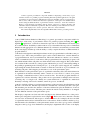
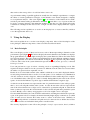
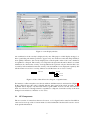
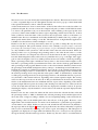
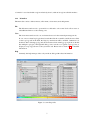
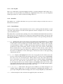
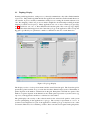
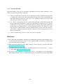
1
CUBE3 — User Manual
Generic Display for Application Performance Data
Version 3.4 / March 28, 2013
Fengguang Song, Felix Wolf, Farzona Pulatova, Markus Geimer, Daniel Becker, Brian Wylie
c 2008
Copyright c 2008-2013
Copyright University of Tennessee
Forschungszentrum J¨ulich GmbH
Contents
1
Introduction
3
2
Using the Display
4
2.1
Basic Principles . . . . . . . . . . . . . . . . . . . . . . . . . . . . . . . . . . .
4
2.2
GUI Components . . . . . . . . . . . . . . . . . . . . . . . . . . . . . . . . . .
5
2.2.1
Tree Browsers . . . . . . . . . . . . . . . . . . . . . . . . . . . . . . .
6
2.2.2
Menu Bar . . . . . . . . . . . . . . . . . . . . . . . . . . . . . . . . . .
7
2.2.3
Color Legend . . . . . . . . . . . . . . . . . . . . . . . . . . . . . . . .
8
2.2.4
Status Bar . . . . . . . . . . . . . . . . . . . . . . . . . . . . . . . . . .
8
2.2.5
Context Menus . . . . . . . . . . . . . . . . . . . . . . . . . . . . . . .
8
Topology Display . . . . . . . . . . . . . . . . . . . . . . . . . . . . . . . . . .
9
2.3
2.3.1
Topology Menu Bar . . . . . . . . . . . . . . . . . . . . . . . . . . . .
10
Abstract
CUBE is a generic presentation component suitable for displaying a wide variety of performance metrics for parallel programs including MPI and OpenMP applications. Program
performance is represented in a multi-dimensional space including various program and system resources. The tool allows the interactive exploration of this space in a scalable fashion
and browsing the different kinds of performance behavior with ease. CUBE also includes a
library to read and write performance data as well as operators to compare, integrate, and
summarize data from different experiments. This user manual provides instructions of how to
use the CUBE display, how to use the operators, and how to write CUBE files.
The CUBE 3 implementation has incompatible API and file format to preceding versions.
1
Introduction
(CUBE Uniform Behavioral Encoding) is a generic presentation component suitable for
displaying a wide variety of performance metrics for parallel programs including MPI [2] and
OpenMP [3] applications. CUBE allows interactive exploration of a multidimensional metric space
in a scalable fashion. Scalability is achieved in two ways: hierarchical decomposition of individual
dimensions and aggregation across different dimensions. All metrics are uniformly accommodated
in the same display and thus provide the ability to easily compare the effects of different kinds of
program behavior.
CUBE
CUBE has been designed around a high-level data model of program behavior called the CUBE per-
formance space. The CUBE performance space consists of three dimensions: a metric dimension,
a program dimension, and a system dimension. The metric dimension contains a set of metrics,
such as communication time or cache misses. The program dimension contains the program’s call
tree, which includes all the call paths onto which metric values can be mapped. The system dimension contains all the control flows of the program, which can be processes or threads depending on
the parallel programming model. Each point (m, c, l) of the space can be mapped onto a number
representing the actual measurement for metric m while the control flow of process/thread l was
executing call path c. This mapping is called the severity of the performance space.
Each dimension of the performance space is organized in a hierarchy. First, the metric dimension
is organized in an inclusion hierarchy where a metric at a lower level is a subset of its parent,
for example, communication time is below execution time. Second, the program dimension is
organized in a call-tree hierarchy. Flat profiles can be represented as multiple trivial call trees
consisting only of a single node. Finally, the system dimension is organized in a multi-level
hierarchy consisting of the levels: machine, SMP node, process, and thread.
CUBE also includes a library to read and write instances of the previously described data model in
the form of an XML file. The file representation is divided into a metadata part and a data part.
The metadata part describes the structure of the three dimensions plus the definitions of various
program and system resources. The data part contains the actual severity numbers to be mapped
onto the different elements of the performance space.
The display component can load such a file and display the different dimensions of the performance space using three coupled tree browsers (Figure 1). The browsers are connected so that the
user can view one dimension with respect to another dimension. For example, the user can click
on a particular metric and see its distribution across the call tree. If the CUBE file contains topological information, the distribution of the performance metric across the topology can be examined
using the CUBE topology view. Furthermore, the display is augmented with a source-code display
3
that can show the exact position of a call site in the source code.
As performance tuning of parallel applications usually involves multiple experiments to compare
the effects of certain optimization strategies, CUBE includes a new feature designed to simplify
cross-experiment analysis. The CUBE algebra [4] is an extension of the framework for multiexecution performance tuning by Karavanic and Miller [1] and offers a set of operators that can
be used to compare, integrate, and summarize multiple CUBE data sets. The algebra allows the
combination of multiple CUBE data sets into a single one that can be displayed like the original
ones.
The following sections explain how to use the CUBE display, how to create CUBE files, and how
to use the algebra and other tools.
2
Using the Display
This section explains how to use the CUBE display component. After a brief description of the
basic principles, different components of the GUI will be described in detail.
2.1
Basic Principles
The CUBE display consists of three tree browsers, each of them representing a dimension of the
performance space (Figure 1). The left tree displays the metric dimension, the middle tree displays
the program dimension, and the right tree displays the system dimension. The nodes in the metric
tree represent metrics. The nodes in the program dimension can have different semantics depending on the particular view that has been selected. In Figure 1, they represent call paths forming
a call tree. The nodes in the system dimension represent machines, nodes, processes, or threads
from top to bottom.
Users can perform two types of actions: selecting a node or expanding/collapsing a node. The
expansion/collapsion behavior for the system tree is different from the other trees because either
all entities of a given level are expanded or none.
Each node is associated with a metric value, which is called the severity and is displayed simultaneously using a numerical value as well as a colored square. Colors enable the easy identification
of nodes of interest even in a large tree, whereas the numerical values enable the precise comparison of individual values. The sign of a value is visually distinguished by the relief of the colored
square. A raised relief indicates a positive sign, a sunken relief indicates a negative sign.
A value shown in the metric tree represents the sum of a particular metric for the entire program,
that is, across all call paths and the entire system. A value shown in the call tree represents the
sum of the selected metric across all processes or threads for a particular call path. A value shown
in the system tree represents the selected metric for the selected call path and a particular system
resource. Briefly, a tree is always an aggregation of all of its neighbor trees to the right.
Note that all the hierarchies in CUBE are inclusion hierarchies, meaning that a child node represents
a part of the parent node. For example, the metric hierarchy might display cache misses as a child
node of cache accesses because the former event is a subset of the latter event. Similarly, in
Figure 2 the call path main contains the call paths main-foo and main-bar as child nodes because
their execution times are included in their parent’s execution time.
The severity displayed in CUBE follows the principle of single representation, that is, within a
4
Figure 1: CUBE display window.
tree each fraction of the severity is displayed only once. The purpose of this display strategy is to
have a particular performance problem to appear only once in the tree and, thus, help identify it
more quickly. Therefore, the severity displayed at a node depends on the node’s state, whether it
is expanded or collapsed. The severity of a collapsed node represents the whole subtree associated
with that node, whereas the severity of an expanded node represents only the fraction that is not
covered by its descendants because the severity of its descendants is now displayed separately. We
call the former one inclusive severity, whereas we call the latter one exclusive severity.
100 main
10 main
30 foo
60 bar
Figure 2: Node of the call tree in collapsed or expanded state.
For instance, a call tree may have a node main with two children main-foo and main-bar (Figure 2).
In the collapsed state, this node is labeled with the time spent in the whole program. In the
expanded state it displays only the fraction that is spent neither in foo nor in bar. Note that the
label of a node does not change when it is expanded or collapsed, even if the severity of the node
changes from exclusive to inclusive or vice versa.
2.2
GUI Components
The GUI consists of a menu bar, three tree browsers, a color legend, and a status bar. In addition,
some tree browsers provides a context menu associated with each node that can be used to access
node-specific information.
5
2.2.1
Tree Browsers
The tree browsers are controlled by the left and right mouse buttons. The left mouse button is used
to select or expand/collapse a node. The right mouse button is used to pop up a context menu with
node-specific information, such as online documentation.
A label in the metric tree shows a metric name. A label in the call tree shows the last callee of a
particular call path. If you want to know the complete call path, you must read all labels from the
root down to the particular node you are interested in. After switching to the region-profile view
(see below), labels in the middle tree denote regions depending on their level in the tree. A label
in the system tree shows the name of the system resource it represents, such as a node name or a
machine name. Processes and threads are usually identified by a number, but it is possible to give
them specific names when creating a CUBE file. The thread level of single-threaded applications
is hidden. Note that all trees can have multiple root nodes.
Each tree view has its own drop-down menu, where it is possible to change the way the severty
values are displayed. The options include: absolute value (default), a root percentage, a selection
percentage, an external percentage, a peer percentage, or a peer distribution. The last two options
are only available for the system tree. The absolute value is the real value measured. When displaying a value as a root percentage, the percentage refers to the value shown at the root of the
metric tree when it is in collapsed state. However, both absolute mode and root percentage mode
have the disadvantage that values can become very small the more you go to the right, since aggregation occurs from right to left. To avoid this problem, the user can switch to selection percentage.
Then, a percentage in the right or middle tree always refers to the selection in the neighbor to the
left, that is, a percentage in the system dimension refers to the selection in the program dimension
and a percentage in the program dimension refers to the selected metric dimension. In this mode
the percentages in the middle and right tree always sum up to one hundred percent. Furthermore, to
facilitate the comparison of different experiments, users can choose the external percentage mode
to display percentages relative to another data set. The external percentage mode is basically like
the normal percentage mode except that the value equal to 100% is determined by another data
set. The peer percentage mode shows the percentage relative to the maximum amount of peer values (all entities of the current leaf level), depending on the current expansion depth. The severity
values for the non-peer nodes are shown as N.A. The peer distribution mode shows the percentage
relative to the maximum and non-zero minimum amount of peer values, depending on the current
expansion depth. The non-peer node severity values and all peers with exact zero values are shown
as N.A. Note that in the absolute mode, all values are displayed in scientific notation. To prevent
cluttering the display, only the mantissa is shown at the nodes with the exponent displayed at the
color legend.
Each tree view also has a status bar, where the left section shows the selected absolute value and
the percentage relative to 100% as defined in the selected percentage mode and the right section
shows the value or range according to which colors are assigned depending on the selected mode.
After opening a data set the middle panel shows the call tree of the program. However, a user
might wish to know which fraction of a metric can be attributed to a particular region regardless
of from where it was called. In this case, the user can switch from the call-tree mode (default) to
the region-profile mode (Figure 3). In the region-profile mode, the call-tree hierarchy is replaced
with a source-code hierarchy consisting of two levels: region, and subregions. The subregions, if
applicable, are displayed as a single child node labeled subregions. A subregions node represents
all regions directly called from the region above. In this way, the user is able to see which fraction
6
of a metric is associated with a region exclusively, that is, without its regions called from there.
2.2.2
Menu Bar
The menu bar consists of three menus, a file menu, a view menu, and a help menu.
File
The file menu can be used to open and close a file and to exit CUBE. It also allows users to
add additional mirrors to the existing ones.
View
The view menu can be used to set a reference data set for the external percentage mode.
If one or more virtual topologies have been defined in the CUBE file, and if the user clicks
on the topology tab in the GUI, the Topology menu item will be enabled. Otherwise it is
disabled. After selecting topolgy tab, the Cartesian-selection dialog pops up if the CUBE file
has multiple topologies. Through this dialog, users can choose a specific topology view to
display in a topology tab next to the system tree tab. Please refer to Section 2.3 for detailed
information.
Help
Currently, the help menu provides only an About dialog with release information.
Figure 3: CUBE flat profile.
7
2.2.3
Color Legend
The color is taken from a spectrum ranging from blue to red representing the whole range of possible values. To avoid an unnecessary distraction, insignificant values close to zero are displayed
in dark gray. Exact zero values just have the background color.
2.2.4
Status Bar
The numbers m × n indicate that there are m processes and for each process there are at most n
threads in the execution.
2.2.5
Context Menus
All tree views provide a context menu that can be used to obtain specific information on each
node. The context menu is accessible via the right mouse button. It displays all or a subset of the
options described below.
The call tree has a context menu consisting of two levels. The first-level menu items are Call site
and Called region. Choosing the Call site menu shows the information related to the call site, and
choosing the Called region menu shows the information related to the region being called by the
call site (i.e., the callee).
Location: Displays the source-code location of a program resource in textual form (i.e., at which
line and in what module). In the module-profile and region-profile modes, it always refers
to the location of its associated region. In the call-tree mode, a call-tree node is usually
associated with two entities: a callsite and the region called by the callsite. By entering a
specific level of the context menu: Callsite or Called region, users are able to check either
the associated call site’s or the called region’s location. For the call site, it shows the call
site’s location where it has been called or its calling region’s location if the line number of
the call site is undefined. For the called region, it shows the location of the region being
called by the call site.
Source code: Displays and highlights the source code of a program resource in the source code
browser. In the module-profile and region-profile modes, it always shows and highlights
the source code of its associated region. In the call-tree mode, since each call-tree node
has a context menu of two levels, by choosing the Call site menu it displays and highlights
the source code of the call site or the block of source code of the calling region. And
by choosing the Called region menu it displays and highlights the block of code of the
region being called by the call site. Note that not all data sets provide sufficient line-number
information to show the correct section of the source code.
Online description: Both metrics and regions can be linked to an online description. For
example, metrics might point to an online documentation explaining their semantics, or regions representing library functions might point to the corresponding library documentation.
Info: A brief description of the selected node supplied by the CUBE data set.
8
2.3
Topology Display
In many parallel applications, each process (or thread) communicates only with a limited number
of processes. The parallel algorithm divides the application domain into smaller chunks known as
sub domains. A process usually communicates with processes owning sub domains adjacent to its
own. The mapping of data onto processes and the neighborhood relationship resulting from this
mapping is called virtual topology. Many applications use one or more virtual topologies (Figure 4) specified as one-, two- or three-dimensional Cartesian grids. The CUBE topology display
shows performance data mapped onto the Cartesian topology of the application. The corresponding grid is specified by two parameters: number of dimensions and size of each dimension.
Figure 4: Topology Display
The display consists of a drop-down menu and the actual Cartesian grid. The Cartesian grid is
presented by planes stacked on top of each other in a three dimensional projection. The number of
planes depends on the number of dimensions in the grid. Each plane is divided into squares. The
number of squares depends on the dimension size. Each square represents a system resource (e.g
a process) of the application and has a coordinate associate with it.
The grid displays the severity of the selected metric in the selected call path for each system
resource participating in the application’s topology. The severity is represented as a color. A
system resource might not be a part of the application’s virtual topology or may have a zero value
for a metric. Therefore, it is sometimes possible to have some uncolored squares in the grid picture.
9
2.3.1
Topology Menu Bar
The menu related to Topology is located in the View Menu. It consists of three submenus: a view
menu, a geometry menu, and a zoom menu.
View: The view menu can be used to choose one of the three possible orientations of the grid. The
coordinate axes at the bottom of the picture indicate the direction of X, Y and Z dimensions
in the three-dimensional space. In case of one- or two- dimensional grids, users are provided
with only one orientation of the grid.
Geometry: Due to varying dimension sizes, planes in the grid might overlap with each other and
the size of the squares might be too small to recognize their color. This may pose a problem
for the user to view the topology information effectively. The geometry menu circumvents
this problem by providing options to scale the picture in various ways. The Angle option
helps the user to adjust the skew of the three-dimensional projection. The Plane Distance
option helps to adjust the inter-plane distance. The Plane Length option helps users scale
the area of each plane.
Zoom: The zoom menu can be used to zoom-in or zoom-out on the grid.
References
[1] K. L. Karavanic and B. Miller. A Framework for Multi-Execution Performance Tuning. Parallel and Distributed Computing Practices, 4(3), September 2001. Special Issue on Monitoring
Systems and Tool Interoperability.
[2] Message Passing Interface Forum. MPI: A Message Passing Interface Standard, June 1995.
http://www.mpi-forum.org.
[3] OpenMP Architecture Review Board. OpenMP Application Program Interface — Version
2.5, May 2005. http://www.openmp.org.
[4] F. Song, F. Wolf, N. Bhatia, J. Dongarra, and S. Moore. An Algebra for Cross-Experiment
Performance Analysis. In Proc. of ICPP 2004, pages 63–72, Montreal, Canada, August 2004.
10