Download Leica TCS SP5 Leica TCS SP5 X User Manual

Leica TCS SP5
Leica TCS SP5 X
User Manual
Published by:
Leica Microsystems CMS GmbH
Am Friedensplatz 3
D-68165 Mannheim (Germany)
http://www.leica-microsystems.com
http://www.confocal-microscopy.com
Responsible for contents: Leica Microsystems CMS GmbH
Copyright © Leica Microsystems CMS GmbH.
All rights reserved.
2
Table of Contents
1.
General .................................................................................................................9
1.1
Copyright.............................................................................................................9
1.2
About this Operating Manual ............................................................................10
2.
Leica TCS SP5 / TCS SP5 X ..............................................................................11
2.1
TCS SP5 system overview ...............................................................................11
2.2
TCS SP5 X system overview ............................................................................12
2.3
Intended Use.....................................................................................................12
2.4
Conformity.........................................................................................................13
2.5
Patents..............................................................................................................14
2.6
Serial Number ...................................................................................................14
2.7
Specifications....................................................................................................15
2.7.1
Dimensions .....................................................................................................15
2.7.1.1
TCS SP5 with inverted microscope ............................................................15
2.7.1.2
TCS SP5 with upright microscope..............................................................15
2.7.1.3
TCS SP5 X with inverted microscope.........................................................16
2.7.1.4
TCS SP5 X with upright microscope ..........................................................16
2.7.2
Electrical Connection Requirements ...............................................................17
2.7.2.1
Electrical connection requirements of supply unit ......................................17
2.7.2.2
Electrical connection requirements of achromatic light laser .....................17
2.7.3
Requirements Regarding Ambient Conditions ................................................18
2.7.4
Permitted Ambient Conditions.........................................................................18
2.7.5
Waste Heat/Required Cooling Performance ...................................................19
2.8
Features............................................................................................................19
2.8.1
Overview of Usable VIS/UV Lasers ................................................................19
2.8.2
Overview of Usable MP Lasers (IR Lasers) ....................................................20
2.8.2.1
Picosecond laser ........................................................................................20
2.8.2.2
Femtosecond laser .....................................................................................21
2.8.3
Overview of Usable VIS/UV Lasers for TCS SP5 X........................................22
2.8.4
Which Laser Class Does the Product Have? ..................................................23
2.8.5
Required Laser Safety Measures....................................................................23
3.
Safety Instructions and their Meanings...........................................................25
3
4.
General Safety Instructions ............................................................................. 27
4.1
Laser Class for VIS and UV Systems............................................................... 27
4.2
Laser Class for MP Systems ............................................................................ 27
4.3
What does the owner/operator have to observe? ............................................ 27
4.4
Safety Instructions for the User ........................................................................ 29
4.5
Operational Reliability ...................................................................................... 29
4.6
Maximum Current Load of the Multiple Socket Outlet at the Supply Unit ........ 30
5.
Safety Devices................................................................................................... 31
5.1
Disconnecting the Power Supply...................................................................... 31
5.2
Detachable-key Switch..................................................................................... 32
5.3
Emissions Warning Indicators .......................................................................... 34
5.4
Remote Interlock Connection on the Supply Unit............................................. 35
5.5
Remote interlock connection on the achromatic light laser ............................. 36
5.6
Remote Interlock Connections on External Lasers .......................................... 37
5.7
Remote interlock jack/interlock connector on the scanner ............................... 37
5.8
Function and Position of Safety Switches ........................................................ 38
5.9
Special Laser Safety Equipment ...................................................................... 39
5.9.1
Laser protection tube and beam stop ............................................................. 39
5.9.2
Shielding in MP Systems (IR Lasers) ............................................................. 40
5.10
Safety labels on the system ............................................................................. 41
5.10.1
Inverted microscope DMI 6000 CS................................................................. 41
5.10.2
Upright microscope DM 5000/6000 CS .......................................................... 43
5.10.3
Scan Head...................................................................................................... 45
5.10.4
Achromatic light laser .................................................................................... 46
5.10.5
External UV laser ........................................................................................... 47
5.10.6
Supply Unit ..................................................................................................... 48
5.10.7
MP beam coupling unit................................................................................... 49
5.10.8
Cover (for Replacement Flange) .................................................................... 50
5.10.9
Mirror Housing ................................................................................................ 51
6.
Safety Instructions for Operating the System................................................ 53
6.1
Requirements Related to the Installation/Storage Location ............................. 53
6.2
General Safety Instructions for Operation ........................................................ 53
6.3
Eye Protection .................................................................................................. 54
6.3.1
MP System with Upright Microscope.............................................................. 54
6.3.2
MP System with Inverted Microscope ............................................................ 54
4
6.3.3
VIS and UV Systems with Inverted or Upright Microscope .............................54
6.4
Specimen Area .................................................................................................55
6.5
Changing Specimens........................................................................................56
6.6
Changing Objectives.........................................................................................57
6.7
Changing the Transmitted-Light Lamp Housing................................................58
6.8
Mirror housing on upright microscope...............................................................60
6.9
Changing Filter Cubes, Beam Splitters or Condenser ......................................62
6.10
Piezo focus on upright microscope ...................................................................63
6.10.1
7.
Objective Change with Piezo Focus Configuration .........................................64
Starting Up the System .....................................................................................65
7.1
Switching On the System ..................................................................................65
7.2
Starting the LAS AF ..........................................................................................70
7.3
Setting Up Users...............................................................................................72
8.
Switching Off the System .................................................................................73
9.
Introduction to LAS AF .....................................................................................75
9.1
General .............................................................................................................75
9.2
Online Help .......................................................................................................75
9.2.1
Structure of the Online Help............................................................................75
9.2.2
Accessing the Online Help ..............................................................................76
9.2.3
Full-text Search with Logically Connected Search Terms...............................76
9.3
9.3.1
Structure of the graphical user interface ...........................................................78
General Structure of the Graphical User Interface..........................................78
9.4
Key Combinations.............................................................................................79
10.
Introduction to Confocal Work .........................................................................81
10.1
Preparation .......................................................................................................81
10.1.1
The Objective ..................................................................................................82
10.1.2
Conventional Microscopy ................................................................................82
10.1.3
Why Scan?......................................................................................................85
10.1.4
How Is an Optical Section Created? ...............................................................86
10.2
Acquiring Optical Sections ................................................................................88
10.2.1
Data Acquisition ..............................................................................................88
10.2.2
Illumination ......................................................................................................90
10.2.3
Beam Splitting .................................................................................................91
10.2.4
Emission Bands ..............................................................................................92
5
10.2.5
The Pinhole and Its Effects............................................................................. 93
10.2.6
Image Detail and Raster Settings................................................................... 95
10.2.7
Signal and Noise ............................................................................................ 99
10.2.8
Profile Cuts ................................................................................................... 101
10.3
Multiparameter Fluorescence......................................................................... 102
10.3.1
Illumination ................................................................................................... 102
10.3.2
Beam Splitting .............................................................................................. 104
10.3.3
Emission Bands............................................................................................ 104
10.3.4
Crosstalk ...................................................................................................... 104
10.3.5
Sequential Scanning .................................................................................... 105
10.3.6
Unmixing ...................................................................................................... 105
10.4
3D Series........................................................................................................ 106
10.4.1
Z-stack.......................................................................................................... 106
10.4.2
Section Thicknesses .................................................................................... 106
10.4.3
Distances...................................................................................................... 107
10.4.4
Data Volumes ............................................................................................... 107
10.4.5
Depictions..................................................................................................... 108
10.4.5.1
Gallery ..................................................................................................... 108
10.4.5.2
Movie ....................................................................................................... 108
10.4.5.3
Orthogonal Projections ............................................................................ 109
10.4.5.4
Rotated Projections ................................................................................. 110
10.5
Time Series .................................................................................................... 110
10.5.1
Scan Speed.................................................................................................. 110
10.5.2
Points ........................................................................................................... 111
10.5.3
Lines............................................................................................................. 111
10.5.4
Planes .......................................................................................................... 111
10.5.5
Spaces (Time-Space)................................................................................... 111
10.5.6
FRAP Measurements ................................................................................... 112
10.6
Spectral Series ............................................................................................... 112
10.6.1
Data Acquisition and Utilization .................................................................... 112
10.6.2
About Spectral Resolution ............................................................................ 112
10.7
11.
Combinatorial Analysis................................................................................... 112
Care and Maintenance .................................................................................... 115
11.1
General........................................................................................................... 115
11.2
Cleaning the Optical System .......................................................................... 115
6
11.3
Cleaning the Microscope Surface ...................................................................116
11.4
Maintaining the Scanner Cooling System .......................................................116
12.
Transport and Disposal...................................................................................117
12.1
Changing the Installation Location..................................................................117
12.2
Disposal ..........................................................................................................117
13.
Contact .............................................................................................................117
14.
Glossary ...........................................................................................................118
15.
Appendix ..........................................................................................................124
15.1
Safety Data Sheets from Third-party Manufacturers.......................................124
15.2
Declaration of conformity ................................................................................129
15.3
People´s Republic of China ............................................................................130
7
8
1. General
1.1
Copyright
The instructions contained in the following documentation reflect state-of-the-art technology
and knowledge standards. We have compiled the texts and illustrations as accurately as
possible. Nevertheless, no liability may be assumed for the accuracy of this manual's
contents. If you have any comments on this operating manual or on any of our other
documentation, we would be pleased to hear from you. The information contained in this
operating manual is subject to change without prior notice.
All rights to this documentation are held by Leica Microsystems CMS GmbH. Adaptation,
translation and reproduction of text or illustrations (in whole or in part) by print, photocopy,
microfilm or other method (including electronic systems) is not allowed without express
written permission from Leica Microsystems CMS GmbH.
Programs such as LAS and LAS AF are protected by copyright laws. All rights reserved.
Reproduction, adaptation or translation of these programs is prohibited without prior written
permission from Leica Microsystems CMS GmbH.
The term "Windows" may be used in the following text without further identification. It is a
registered trademark of the Microsoft Corporation. Otherwise, no inference with regard to the
free usability of product names may be drawn from the use of those names. All other brand
names and product names in this document are brands, service marks, trademarks or
registered trademarks of the respective manufacturers.
Made in Germany.
© Copyright Leica Microsystems CMS GmbH.
All rights reserved.
9
1.2
About this Operating Manual
Whenever this manual refers to the "system" or provides no specific information for
one of the systems, then the notes, instructions and information applies to
TCS SP5 and TCS SP5 X.
The main focus of this operating manual is directed to the safety notes that must be strictly
adhered to when working with the Leica TCS SP5 and Leica TCS SP5 X.
In addition, this operating manual provides a rough overview of the operating principle of
laser scanning microscopes. It presents you with the first steps for activating and
commissioning the system and provides important information about the Leica Application
Suite Advanced Fluorescence (LAS AF) software.
The system is delivered with the latest version of the licensed LAS AF. To maintain
information on the most current level, the description of software functions was intentionally
omitted from this operating manual. Instead, reference is made to the online help of the LAS
AF in which you can find up-to-date explanations and instructions for the corresponding
software functions.
Please read the chapter "Introduction to the LAS AF" in this operating manual to familiarize
yourself with its setup and operation. Additional information about specific functions can then
be found in the online help.
10
2. Leica TCS SP5 / TCS SP5 X
2.1
TCS SP5 system overview
Figure 1: TCS SP5 system components (overview)
1
2
3
4
5
6
TCS SP5 Scanner
Main switch board
TCS workstation
Supply unit
Control panel
Microscope
11
2.2
TCS SP5 X system overview
Figure 2: TCS SP5 X system components (overview)
1
2
3
4
5
6
7
2.3
TCS SP5 X scanner
Main switch board
TCS workstation
Supply unit
Control panel
Microscope
Achromatic light laser
Intended Use
The system was designed for confocal scanning (laser scanning images) of fluorescencemarked living and fixed specimens as well as for quantitative measurements in the area of
life science.
This system is intended for use in a lab.
Applications of in-vitro diagnostics in accordance with MPG (German Medical Devices Act)
are excluded from proper intended use.
12
The manufacturer assumes no liability for damage caused by, or any risks arising from, use
of the microscopes for purposes other than those for which they are intended, or not using
the microscopes within the specifications of Leica Microsystems CMS GmbH. In such cases,
the Declaration of Conformity shall be invalid.
2.4
Conformity
This device has been tested and meets the requirements of the following standards:
IEC/EN 61010-1
IEC/EN 60825-1
IEC/EN 61326
"Safety requirements for electrical equipment for measurement, control
and laboratory use"
"Safety of laser products, Part
1: Equipment classification, requirements and user's guide"
"Electrical Equipment for Measurement, Control and Laboratory Use −
EMC Requirements" (Class A).
This is a Class A instrument for use in buildings that do not include
domestic premises and buildings not directly connected to a lowvoltage power supply network that supplies buildings used for
domestic purposes.
IEC/EN 61000-3-2
"Electromagnetic Compatibility (EMC)"
Part 3-2: Limits — Limits for harmonic currents
IEC/EN 61000-3-3
"Electromagnetic Compatibility (EMC)"
Part 3-3: Limits — Limitation of voltage fluctuations and flicker in lowvoltage supply systems.
The declaration of conformity for the system is located in the appendix of this operating
manual.
For use in the USA:
CDRH 21 CFR 1040.10:
U.S. laser products Food and Drug Administration (FDA)
(”Complies with FDA performance standards for laser products
except for deviations pursuant to laser notice No. 50, dated 26
July, 2001.
For the USA (area of validity of the CDRH/FDA), the designations of the laser class are to be
changed in the text from 3B to IIIb and Class 4 to IV.
13
2.5
Patents
The Leica TCS SP5 product is protected by the US patents:
5,886,784; 5,903,688; 6,137,627; 6,222,961; 6,285,019; 6,311,574; 6,355,919; 6,423,960;
6,433,814; 6,444,971; 6,466,381; 6,510,001; 6,614,526; 6,654,165; 6,657,187; 6,678,443;
6,687,035; 6,738,190; 6,754,003; 6,801,359; 6,831,780; 6,850,358; 6,867,899.
Further patents are pending.
The Leica TCS SP5 X protect by the US patents:
5,886,784; 5,903,688; 6,137,627; 6,222,961; 6,285,019;
6,433,814; 6,444,971; 6,466,381; 6,510,001; 6,567,164;
6,654,166; 6,657,187; 6,678,443; 6,687,035; 6,710,918;
6,801,359; 6,806,953; 6,831,780; 6,850,358; 6,867,899;
6,961,124; 7,005,654; 7,092,086; 7,110,645; 7,123,408.
Further patents are pending.
2.6
6,311,574;
6,611,643;
6,738,190;
6,888,674;
6,355,919;
6,614,526;
6,754,003;
6,898,367;
Serial Number
The serial number of your system is located on the rear side of the scanner:
Figure 3: Rear side of scanner – label with serial number
14
6,423,960;
6,654,165;
6,796,699;
6,958,858;
2.7
Specifications
2.7.1
Dimensions
2.7.1.1 TCS SP5 with inverted microscope
1400 mm
600 mm
730 mm
2540 mm
1200 mm
Figure 4: Dimensions of TCS SP5 with inverted microscope
2.7.1.2 TCS SP5 with upright microscope
1490 mm
730 mm
600 mm
2400 mm
1200 mm
Figure 5: Dimensions of TCS SP5 with upright microscope
15
2.7.1.3 TCS SP5 X with inverted microscope
Figure 6: Dimensions of TCS SP5 X with inverted microscope
2.7.1.4 TCS SP5 X with upright microscope
Figure 7: Dimensions of TCS SP5 X with upright microscope
16
2.7.2
Electrical Connection Requirements
The building installation must feature three separate power connections with the following
fuse protection:
• 3 x 100 V - 120 V power supply at 20 A
or
•
3 x 200 V - 240 V power supply at 12 - 16A
For the specifications of external lasers such as UV and MP lasers, please refer to the
manufacturer's documentation.
2.7.2.1 Electrical connection requirements of supply unit
Supply voltage:
100 - 240 V AC ± 10 %
Frequency:
50/60 Hz
Power consumption:
3200 VA
Overvoltage category:
II
2.7.2.2
Electrical connection requirements of achromatic light laser 1
Supply voltage:
100 - 240 V AC ± 10 %
Frequency:
50/60 Hz
Power consumption:
2.2 A
Overvoltage category:
II
Fuse
2x T4A, 250V AC
1
Applies only to the TCS SP5 X system.
17
2.7.3
Requirements Regarding Ambient Conditions
Do not expose the system to drafts.
Ensure that the system is not installed next to air conditioners or ventilation systems. For this
reason, the installation location should be carefully planned.
Ensure that the environment is as dust-free as possible.
Also read the notes on protection against dust in Chapter 11 Care and Maintenance
Installing the system in darkened rooms is also advisable.
The system requires doors with inside widths of 1.0 m for installation, maintenance and
transport.
With regard to the load-bearing capacity of the floor, note that the system will apply a static
load of 200 kg/m².
Ensure that the environment is as vibration-free as possible.
2.7.4
Permitted Ambient Conditions
Permissible temperature range for operation:
+18 to +25 ºC
Temperature range for optimum optical
behavior:
+22 °C ±1 °C
Permitted relative humidity:
20 - 80% (non-condensing)
Permitted vibrations:
Frequency range [5 Hz–30 Hz]:
Frequency range [> 30 Hz]:
< 30 μm/s (RMS)
< 60 μm/s (RMS)
Pollution degree:
Class 2
18
2.7.5
Waste Heat/Required Cooling Performance
The TCS SP5 system has a maximum power consumption of 3.2 kW (VIS system) or 6.2 kW
(MP system).
The TCS SP5 X has a maximum power consumption of 3.4 kW.
For the specifications of external lasers such as UV and MP lasers, please refer to the
manufacturer's documentation.
2.8
Features
2.8.1
Overview of Usable VIS/UV Lasers
The Leica TCS SP5 features a combination of the lasers listed below.
Laser type
Wavelength
[nm]
Maximum
luminous power
at laser output
[mW]
Maximum
luminous power
in focal plane
[mW]
Pulse duration
Diode 405
405
< 120
<7
Continuous wave
(cw)
Diode 405 p
405
< 5 (mean
power)
< 0.3 (mean
power)
pulsed, 60 ps
DPSS 445
445
< 75
<7
Continuous wave
(cw)
Ar
458, 476, 488,
< 200
496, 514
< 50
Continuous wave
(cw)
Ar, external
458, 476, 488,
< 500
496, 514
< 125
Continuous wave
(cw)
HeNe
543
< 1.5
< 0.5
DPSS 561
561
< 100
< 12
HeNe
594
<4
<1
HeNe
633
< 15
<5
UV, external
355
< 500
< 18
Continuous wave
(cw)
Continuous wave
(cw)
Continuous wave
(cw)
Continuous wave
(cw)
Continuous wave
(cw)
Table 1: Usable lasers for TCS SP5 (without MP)
19
The components for laser safety are designed only for the laser variants listed.
2.8.2
Overview of Usable MP Lasers (IR Lasers)
Furthermore, the MP system may contain additional VIS/UV lasers (see the table for usable
VIS/UV lasers).
2.8.2.1 Picosecond laser
Laser type
Luminous
Wavelength
power at laser
[nm]
output [W]
Luminous
power in focal
plane [W]
Pulse duration
MaiTai ps
780 - 920
< 1.2
< 0.6
pulsed, 1.0 - 1.5 ps
MaiTai ps
wideband
710 - 950
< 2.5
< 1.2
pulsed, 1.0 - 1.5 ps
MaiTai ps
broadband
710 - 990
< 2.5
< 1.2
pulsed, 1.0 - 1.5 ps
MaiTai ps HP
690 - 1040
< 3.0
< 1.9
pulsed, 1.0 - 1.5 ps
Chameleon ps
Ultra
690 - 1020
<4
< 1.9
pulsed, 1.0 - 1.5 ps
Chameleon ps
Ultra I
690 - 1040
<4
< 1.9
pulsed, 1.0 - 1.5 ps
Chameleon ps
Ultra II
680 - 1080
<4
< 1.9
pulsed, 1.0 - 1.5 ps
Table 2: Usable MP lasers for TCS SP5 and TCS SP5 X
20
2.8.2.2 Femtosecond laser
Laser type
Luminous
Wavelength
power at laser
[nm]
output [W]
Luminous
power in focal
plane [W]
Pulse duration
MaiTai fs
780 - 920
< 1.2
< 0.6
pulsed, 80 fs
MaiTai fs
wideband
710 - 950
< 2.5
< 1.2
pulsed, 80 fs
MaiTai fs
broadband
710 - 990
< 2.5
< 1.2
pulsed, 80 fs
MaiTai fs HP
690 - 1040
< 3.0
< 1.9
pulsed, 100 fs
MaiTai HP
Deep See
690 – 1040
< 3.0
< 1.9
pulsed, 100 fs
Chameleon fs
Ultra
690 - 1020
<4
< 1.9
pulsed, 140 fs
Chameleon fs
Ultra I
690 - 1040
<4
< 1.9
pulsed, 140 fs
Chameleon fs
Ultra II
690 - 1080
<4
< 1.9
pulsed, 140 fs
Chameleon
Vision I
690 – 1040
< 4.0
< 1.9
pulsed, 140 fs
Chameleon
Vision II
680 – 1080
< 4.0
< 1.9
pulsed, 140 fs
680 - 1080
< 4.0
< 1.9
pulsed, 140 fs
1000 - 1600
< 1.6
< 0.8
pulsed > 100 fs
Chameleon
Compact OPO
Table 3: Usable MP lasers for TCS SP5 and TCS SP5 X
The components for laser safety are designed only for the laser variants listed.
21
2.8.3
Overview of Usable VIS/UV Lasers for TCS SP5 X
The Leica TCS SP5 X features a combination of the lasers listed below.
Laser type
Wavelength
[nm]
Maximum
luminous power
at laser output
[mW]
Maximum
luminous power
in focal plane
[mW]
Pulse duration
Diode 405
405
< 120
<7
Continuous wave
(cw)
Diode 405 p
405
< 5 (mean
power)
< 0.3 (mean
power)
pulsed, 60 ps
UV, external
355
< 500
< 18
Ar
458, 476, 488,
< 200
496, 514
< 50
488 solid-state
488
< 470
< 70
470 – 670
< 500
< 50
laser
Achromatic
light laser
Continuous wave
(cw)
Continuous wave
(cw)
Continuous wave
(cw)
Pulsed
Table 4: Usable lasers for TCS SP5 X
The components for laser safety are designed only for the laser variants listed.
22
2.8.4
Laser
variant
Which Laser Class Does the Product Have?
Wavelength range
Configuration
Laser class
VIS
Combination of lasers
from Chapter 2.8.3 or 2.8.1
400 - 700 nm,
(without lasers having
(visible laser radiation)
wavelengths of
350 - 400 nm)
3B / IIIb
UV
350 - 700 nm,
(visible and invisible
laser radiation)
Combination of lasers
from Chapter 2.8.3 or 2.8.1
(VIS and UV lasers)
3B / IIIb
MP
350 - 1600 nm,
(visible and invisible
laser radiation)
Combination of lasers from
chapter 2.8.1 (VIS/UV Laser),
chapter 2.8.2 (IR Laser) or
chapter C2.8.3 (VIS/UV Laser)
2.8.5
4 / IV
Required Laser Safety Measures
Please observe the laser safety measures for laser class 3B / IIIb (VIS and UV systems) or
laser class 4 / IV (MP systems) in accordance with applicable national and federal
regulations. The owner/operator is responsible for observing the laser safety regulations.
23
24
3. Safety Instructions and their Meanings
DANGER
This kind of warning alerts you of an operating procedure, practice, condition, or
instruction in the operating manual that must be strictly observed and followed, as
otherwise you expose yourself to the risk of fatal injury.
WARNING! LASER RADIATION
A laser warning points out an operation, a process, a condition or an instruction
that must be observed strictly to prevent serious eye injuries to the persons using
the system.
WARNING! ELECTRICAL VOLTAGE
A high-voltage warning points out an operation, a process, a condition or an
instruction that must be observed strictly to prevent possible injury or death of the
persons using the system.
WARNING! HARMFUL SUBSTANCES
A harmful substances warning points out a substance that can be harmful to your
health.
CAUTION
A safety instruction points out an operation, a process, a condition or an
instruction that must be observed strictly to prevent severe damage to the system
or loss of data.
WEARING PROTECTIVE EYEWEAR
This mandatory sign draws your attention to the fact that suitable eye protection
gear must be worn when commissioning and operating the system. Failure to
heed this warning may lead to serious and irreversible eye injuries.
OBSERVE INSTRUCTIONS IN OPERATING MANUAL
This mandatory sign draws your attention to the fact that the safety notes and
regulations stipulated in the operating manual must be observed for the secure
and interference-free operation of the system. The operating manual, in particular
the safety notes, must be observed by all people who are working with the system.
25
Notes either contain additional information on a specific topic or special
instructions on the handling of the product.
26
4. General Safety Instructions
4.1
Laser Class for VIS and UV Systems
In accordance with IEC/EN 60825-1, this system is a laser product of Class 3B / IIIb.
Never expose eyes or skin to direct radiation! The laser light can cause permanent
eye damage!
4.2
Laser Class for MP Systems
In accordance with IEC/EN 60825-1, this system is a laser product of Class 4 / IV.
Never expose eyes or skin to direct or indirect radiation! Laser light can cause
permanent eye damage and skin injuries!
4.3
What does the owner/operator have to observe?
The owner/operator of this product is responsible for proper and safe operation and safe
maintenance of the system and for following all applicable safety regulations.
The owner/operator is fully liable for all consequences resulting from the use of the system
for any purposes other than those listed in the operating manual or the online help.
This laser product may be operated only by persons who have been instructed in
the use of the system and the potential hazards of laser radiation.
The owner/operator is responsible for performing and monitoring suitable safety
measures (according to IEC/EN 60825-1 and the corresponding national
regulations).
27
All safety devices, safety locks, and safety systems of the laser product must be in
an operational state.
Deactivating or damaging these safety devices or any intervention in any of these
safety devices may lead to serious eye injuries, physical injuries or property
damage. In these cases, Leica Microsystems CMS GmbH shall not assume any
liability.
The owner/operator is responsible for naming a laser safety officer or a laser
protection advisor (according to the standard IEC/EN 60825-1: "Safety of laser
products, Part 1: Classification of systems, requirements and user guidelines" and
the respective national regulations).
Repairs and servicing may only be performed by authorized Leica Microsystems
CMS GmbH service personnel.
The owner/operator is fully liable for all consequences resulting from the use of the
system if it is opened, improperly serviced or repaired by persons other than
authorized Leica service representatives.
If repairs or service measures are performed that require opening parts of the
housing, only trained Leica service technicians may occupy the room in which the
system is located.
Do not connect any external equipment or other components.
Connect to the product only those electrical devices that are listed in the operating
manual. Otherwise, please contact your local Leica service agency or Leica
Microsystems CMS GmbH.
Leica Microsystems CMS GmbH shall not be liable for damages resulting from
nonobservance of the above information. The above information does not, in any way,
implicitly or explicitly, modify the warranty and liability clauses contained in the general terms
and conditions of Leica Microsystems CMS GmbH.
28
4.4
Safety Instructions for the User
Read and observe the safety instructions in the operating manual and the safety labels
located on the system. Failure to observe the safety instructions may lead to serious injuries
and to significant damages to the system and loss of data.
The instrument is a Class 3B or 4 laser product (depending on the laser used).
This laser product may be operated only by persons who have been instructed in
the use of the system and the potential hazards of laser radiation.
Before carry out operating steps with the system for the first time, first read the
corresponding
description
of
the
function
in
the
online
help.
For an overview of the individual functions, refer to the table of contents of the
online help.
As it is impossible to anticipate every potential hazard, please be careful and apply common
sense when operating this product. Observe all safety precautions relevant to Class 3B/IIIb
lasers and Class 4/IV lasers for MP systems.
Do not deviate from the operating and maintenance instructions provided herein.
The failure to observe these instructions shall be exclusively at the operator's own risk and
may void the warranty.
4.5
Operational Reliability
This instrument must not be used together with life-support systems such as those
found in intensive-care wards.
This instrument may only be used with a grounded AC power supply.
Contact with liquids or the entry of liquids into the housing must be avoided.
29
4.6
Maximum Current Load of the Multiple Socket Outlet at the Supply Unit
The total power consumption of all loads connected to the multiple socket outlet (Figure 8)
must not exceed
800 VA.
The terminals are intended for:
•
TCS workstation
•
Monitor 1
•
Monitor 2
•
Microscope
Figure 8: Multiple socket outlet, rear side of supply unit
30
5. Safety Devices
5.1
Disconnecting the Power Supply
The main circuit breaker is located on the right rear side of the supply unit. It is used to deenergize the complete system using a single switch (Figure 9).
The main circuit breaker functions as a switch and as an overcurrent fuse.
The main circuit breaker is not to be used as the regular on/off switch for the system.
The supply unit must be set up so that the main circuit breaker is freely accessible at all
times.
Figure 9: Supply unit with main circuit breaker
31
5.2
Detachable-key Switch
The detachable-key switch for protection against unauthorized use of the laser products is
located on the main switch board (see Figure 10).
Figure 10: Detachable-key switch for the internal lasers
The detachable-key switch for protection against unauthorized use of the external achromatic
light laser is located on the front of the achromatic light laser (see Figure 11).
Figure 11: Detachable-key switch for the achromatic light laser
32
The key switch for protection against unauthorized use of the external UV laser is located on
the front of the power supply (see Figure 12).
Figure 12: Key switch for the external UV laser
For other external lasers, please refer to the operating manual supplied by the
laser manufacturer for the position of the detachable-key switches.
33
5.3
Emissions Warning Indicators
The operational readiness of lasers located in the supply unit is signaled by an emission
warning indicator (Figure 13). The emission warning indicator is located above the
detachable-key switch and is yellow when lit.
The emission warning indicator of the achromatic light laser is located on the front of the
achromatic light laser (see Figure 14) and is red when lit.
As soon as the emission warning indicator of the lasers is lit, it is possible from a functional
standpoint that laser radiation is present in the specimen area.
Figure 13: Emission warning indicators on the main switch board
Figure 14: Emission warning indicator at the achromatic light laser
Figure 15: Emission warning indicator on power supply of the external UV laser
34
Immediately disconnect the system from the power supply if any of the following
occur:
•
The emission warning indicator is not lit after being switched on
using the detachable-key switch.
•
The indicator continues to be lit after being switched off using the
keyswitch
•
Scanning of the specimen is not activated after being switched on
properly (laser radiation in the specimen area).
Contact Leica Service immediately.
For other external lasers, please refer to the operating manual supplied by the
laser manufacturer for the position of the emission warning indicator.
5.4
Remote Interlock Connection on the Supply Unit
The remote interlock jack is located on the rear side of the supply unit (12 V DC operating
voltage, Figure 16).
The remote interlock plug, which contains a shorting bridge, is connected to this jack.
Remote interlock devices such as those connected to the room, the door or other onsite
safety interlock systems can also be connected to the remote interlock connector. The laser
beam path is interrupted if the contact is open.
The overall length of the cable between the two connecting pins of the remote interlock
connector must not exceed 10 m.
Figure 16: Remote Interlock Connection on the Supply Unit
35
5.5
Remote interlock connection on the achromatic light laser 2
The remote interlock connection is located on the rear side of the achromatic light laser (12 V
DC operating voltage, see Figure 17).
If the white light laser is operated as a component of the TSC SP5 X system, you
have to use the remote interlock jack on the supply unit (see chapter 5.4)! The
remote interlock plug (shorting bridge) must be connected to the remote interlock
jack of the white light laser.
If you operate the white light laser separately (without connecting it to the TCS
SP5 system), you have to use the remote interlock jack on the white light laser
(see Figure 17) for connecting remote interlocks.
Remote interlock devices such as those connected to the room, the door or other onsite
safety interlock systems can also be connected to the remote interlock connector. The laser
beam path is interrupted if the contact is open.
Figure 17: Remote interlock connection at the achromatic light laser
2
Applies only to the TCS SP5 X system.
36
5.6
Remote Interlock Connections on External Lasers
For external lasers, please refer to the operating manual supplied by the laser
manufacturer for the position of the remote interlock connection.
5.7
Remote interlock jack/interlock connector on the scanner
The interlock jack is located on the rear side of the scanner (operating voltage:
12 V DC, Figure 18).
For laser safety reasons, the inverted microscope must be connected to this connection or, if
an upright microscope is used, the mirror housing. This ensures that the safety switch of the
microscope is integrated in the interlock circuit.
Figure 18: Location of the interlock jack
37
5.8
Function and Position of Safety Switches
When the safety switches are released, the light path of the laser beam is interrupted.
Figure 19: Position of the transmitted-light illumination arm (1) and switching from scan mode
to eyepiece (2).
Type of
microscope
Activated if:
1
Transmitted-light
illuminator arm
Inverted
microscope DMI
6000 CS
The illuminator
Prevents laser light
arm is tilted (e.g.
while working on the
for working on the
specimen.
specimen).
2
Motorized
changeover
between scanning
mode and
eyepiece
Inverted
microscope DMI
6000 CS
Prevents stray light if
The deflection
the user switches
mirror for the
from confocal
scanner is swung
observation to
out by motor.
eyepiece observation.
Position Activated by:
38
Function
5.9
Special Laser Safety Equipment
5.9.1
Laser protection tube and beam stop
On inverted microscopes, the safety beam guide and the beam stop serve as protection
against laser radiation emission and are located between the condenser base and the
transmitted-light detector (see Figure 20).
1
Laser protection tube
2
Beam stop
(illustrated is the version of the beam
stop for MP systems)
3
Condenser base
Figure 20: Inverted microscope
If you reorder a condenser base (Figure 20, item 3), be aware that the condenser
base is delivered without the beam stop (Figure 20, item 2).
The existing beam stop (Figure 20, item 2) must always be reinstalled. Please
consult the microscope's operating manual provided.
When using a condenser base with filter holder, always make sure that unused
filter holders are swung out of the beam path, and that the
laser protection tube covers the beam path.
When equipping multiple filter holders with filters, do so from bottom to top so that
the laser protection tube can cover the beam path to the greatest possible extent.
Do not swing in the filters during the scanning operation.
39
5.9.2
Shielding in MP Systems (IR Lasers)
The light of all employed VIS lasers (wavelength range 400 - 700 nm, visible spectrum) and
UV lasers (wavelength range < 400 nm, invisible) is fed through a fiber optic cable and,
therefore, completely shielded until it leaves the microscope objective and reaches the
specimen.
For systems with infrared laser (wavelength range > 700 nm), the beam is passed through a
safety beam guide and, if necessary, also passed through a fiber optic cable (Figure 21).
This shields the laser beam until it leaves the microscope objective and reaches the
specimen.
Figure 21: Safety beam guide (1) and IR laser (2)
40
5.10
Safety labels on the system
The corresponding safety labels are selected dependent on the laser configuration (VIS, UV,
MP) and attached in the following locations either in the English or German language.
5.10.1
Inverted microscope DMI 6000 CS
Angled rear view of right side of microscope:
Figure 22: Safety label for inverted microscope DMI 6000 CS
41
Angled front view of right side of microscope:
Figure 23: Safety label for inverted microscope DMI 6000 CS
42
5.10.2
Upright microscope DM 5000/6000 CS
Angled front view of right side of microscope:
Figure 24: Safety label for upright microscope DM 5000/6000 CS
43
Rear view of microscope:
Figure 25: Safety label for upright microscope DM 5000/6000 CS
44
5.10.3
Scan Head
Angled front view of left side of scan head:
Figure 26: Safety label for the scanner
45
5.10.4
Achromatic light laser 3
Rear side of achromatic light laser:
Figure 27: Safety label on the rear side of the white light laser
3
Applies only to the TCS SP5 X system.
46
5.10.5
External UV laser4
Figure 28: Safety label on external UV laser
4
Applies only to systems with an external UV laser.
47
5.10.6
Supply Unit
View of supply unit:
Figure 29: Safety label for the TCS SP 5 supply unit (front side)
48
5.10.7
MP beam coupling unit
Angled front view of the right side of the MP beam coupling unit:
Figure 30: Safety label for the MP beam coupling unit (top side)
49
5.10.8
Cover (for Replacement Flange)
Front view of cover:
Figure 31: Cover for replacement flange
If the replacement flange for transmitted light is not equipped with a functional module such
as a lamp housing, a cover must be placed over the opening for laser safety reasons.
50
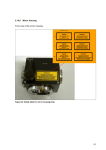
5.10.9
Mirror Housing
Front view of the mirror housing:
Figure 32: Safety label for mirror housing (top)
51
52
6. Safety Instructions for Operating the System
6.1
Requirements Related to the Installation/Storage Location
This device was designed for use in a lab and may not be set up in areas with
medical devices serving as life-support systems such as intensive-care wards.
This equipment is designed for connection to a grounded (earthed) outlet. The
grounding type plug is an important safety feature.
To avoid the risk of electrical shock or damage to the instrument, do not disable
this feature.
To avoid the risk of fire hazard and electrical shock, do not expose the unit to rain
or humidity.
Do not open the cabinet. Do not allow any liquid to enter the system housing or
come into contact with any electrical components. The instrument must be
completely dry before connecting it to the power supply or turning it on.
6.2
General Safety Instructions for Operation
Do not look into the eyepieces during the scanning operation.
Do not look into the eyepieces when switching the beam path in the microscope.
Never look directly into a laser beam or a reflection of the laser beam. Avoid all
contact with the laser beam.
Never deactivate the laser protection devices. Please read the chapter "Laser
Protection Devices" to familiarize yourself with the safety devices of the system.
53
Do not introduce any reflective objects into the laser beam path.
Be sure to follow the included operating instructions for the microscope.
6.3
Eye Protection
6.3.1
MP System with Upright Microscope
Wearing safety goggles (order number: 156502570) is compulsory. Appropriate
safety goggles for IR laser radiation are provided with the system when delivered.
These safety goggles do not offer any protection against visible laser radiation
(visible spectrum).
During the scanning operation, all persons present in the room must wear safety
goggles.
The IR laser beam can be deflected or scattered by the specimen or objects moved into the
specimen area. Therefore, it is not possible to completely eliminate hazards to the eye from
IR laser radiation.
The supplied safety goggles only provide safe protection against the infrared lasers supplied
by Leica Microsystems CMS GmbH.
6.3.2
MP System with Inverted Microscope
It is not necessary to wear eye protection. If the device is used as prescribed and the safety
instructions are observed, the limit of the laser radiation is maintained so that eyes are not
endangered.
6.3.3
VIS and UV Systems with Inverted or Upright Microscope
It is not necessary to wear eye protection. If the device is used as prescribed and the safety
instructions are observed, the limit of the laser radiation is maintained so that eyes are not
endangered.
54
6.4
Specimen Area
The light of all employed VIS lasers used (wavelength range 400 - 700 nm, visible spectrum
) and UV lasers (wavelength range < 400 nm, invisible) is fed through a fiber optic cable and,
therefore, completely shielded until it leaves the microscope objective and reaches the
specimen. The beam divergence, depending on the objective used, is up to 1.16 rad.
Figure 33: Specimen area of upright and inverted microscope
During the scanning operation, the laser radiation is accessible after exiting the
objective in the specimen area of the laser scanning microscope.
This circumstance demands special attention and caution. If the laser radiation
comes in contact with the eyes, it may cause serious eye injuries. For this reason,
special caution is absolutely necessary as soon as one or more of the laser
emission warning indicators are lit.
If the system is used as prescribed and the safety instructions are observed during
operation, there are no dangers to the operator. Always keep your eyes at a safe
distance of at least 20 cm from the opening of the objective.
55
6.5
Changing Specimens
Never change specimens during a scanning operation.
To change specimens, proceed as follows:
Upright microscope
Inverted microscope
Finish the scanning operation.
Finish the scanning operation.
Ensure that no laser radiation is present in Ensure that no laser radiation is present in
the specimen area.
the specimen area.
Tilt the transmitted-light arm back.
Exchange the specimen.
Insert the specimen correctly into the
specimen holder.
Exchange the specimen.
Insert the specimen correctly into the
specimen holder.
Tilt the transmitted-light arm back into the
working position.
56
6.6
Changing Objectives
Do not change objectives during a scanning operation.
To change objectives, proceed as follows:
1. Finish the scanning operation.
2. Switch off the internal lasers using the detachable-key switch.
3. If any external lasers are present, switch them off with their detachable-key switch
or as described in the operating manual of the laser manufacturer.
4. Rotate the objective nosepiece so that the objective to be changed is swiveled out
of the beam path and points outward.
5. Exchange the objective.
All unoccupied positions in the objective nosepiece must be closed using the
supplied caps.
For MP systems, dry objectives (air objectives) may not be used with a numerical
aperture (NA) larger than 0.85. This does not apply to immersion objectives (oil,
water).
If a piezo focus is installed in your system, please also observe the safety notes
related to changing objectives with a piezo focus in 6.10.1.
57
6.7
Changing the Transmitted-Light Lamp Housing
If no transmitted-light lamp housing is connected, to protect from the potential escape of
laser radiation, the opening (Figure 35 or Figure 36) must be securely sealed with the cover
(Figure 34) that accompanies the system.
Figure 34: Cover
To prevent the emission of laser radiation, do not switch the lasers on without a
lamp housing or cover on the microscope.
Figure 35: Port for connecting the transmitted-light lamp housing on the inverted microscope
58
Figure 36: Port for connecting the transmitted-light lamp housing or mirror housing on the
upright microscope
If your microscope features a transmitted-light lamp housing that you would like to replace,
proceed as follows:
1. Switch off the lasers.
2. Disconnect the lamp housing from the power supply.
3. Remove the lamp housing.
4. Modify the lamp housing as needed.
5. After finishing the tasks, screw the new lamp housing back onto the microscope.
59
6.8
Mirror housing on upright microscope
If a mirror housing is not connected to the upright microscope, the opening must be tightly
covered using the cap provided with the system to prevent any laser radiation from escaping
(Figure 37).
Figure 37: Cover
To prevent the emission of laser radiation, do not switch the lasers on without a
mirror housing or cover on the microscope.
If your upright microscope is equipped with a mirror housing, note the following:
60
•
If the mirror housing is removed, you must the close off the port on the
microscope (Figure 36) using the cover (Figure 37).
•
The interlock jack on the mirror housing (see Figure 38, item 1) must be
connected to the scan head at all times.
•
The unused output on the mirror housing must be covered with the cover
provided (see Figure 38, item 3).
When installing the cover (Figure 38, item 3), ensure that the button (Figure 38,
item 2) is pressed by the cover.
Figure 38: Mirror housing on upright microscope
61
6.9
Changing Filter Cubes, Beam Splitters or Condenser
Do not change any filter cubes or beam splitters during a scanning operation.
In LAS AF, set the operating voltage of all external detectors to 0 V and disable
them using the checkbox. If the detectors are not de-energized, they could be
damaged by the infiltration of ambient light.
To change filter cubes or beam splitters proceed as follows:
Upright microscope
Inverted microscope
Finish the scanning operation.
Finish the scanning operation.
In LAS AF, set the operating voltage of all
external detectors to 0 V.
In LAS AF, set the operating voltage of all
external detectors to 0 V.
Remove the cover of the fluorescence
module
(see operating manual for microscope).
Pull out the fluorescence module.
Remove the filter cube/beam splitter.
Remove the filter cube/beam splitter.
Insert the desired
filter cube/beam splitter.
Insert the desired
filter cube/beam splitter.
Reattach the cover to the front of the
fluorescence module.
Reinsert the fluorescence module.
Never disconnect a fiber optic cable.
Never remove the scanner from the microscope during operation.
Before removing the scanner, the system must be completely switched off.
Do not use an S70 microscope condenser. The large working distance and the low
numerical aperture of the S70 microscope condenser could pose a hazard due to
laser radiation. Therefore, only S1 and S28 Leica microscope condensers should
be used.
62
6.10
Piezo focus on upright microscope
Figure 39: Piezo focus on objective nosepiece
If a piezo focus is installed on your system, please also observe the following safety notes:
Before switching the system on or launching the LAS AF software, ensure that
there is no slide or specimen on the stage and that the stage is in its lowest
possible position.
The slide or objective may otherwise be damaged or destroyed by the initialization
of the piezo focus when starting the system/software.
The objective can be moved by 150 µm in either direction. The total travel is 300 µm.
Piezo focus controller display:
Upper position:
350 µm
Middle position:
200 µm
Lowest position:
50 µm
xz-scan range:
250 µm
Figure 40: Piezo focus controller
Do not make any adjustments to the piezo focus controller, as it has already been
optimally set up by Leica Service.
63
Figure 41: Spacer on objective
Please note that the focus position of an objective with piezo focus is 13 mm lower
than those without piezo focus. A spacer (Figure 41) is installed on all other
objectives to ensure the same focal plane.
6.10.1
Objective Change with Piezo Focus Configuration
Do not change objectives automatically! The automatic motion may damage the
cable of the piezo focus.
In addition to the regular procedure (see chapter 6.6) the stage must be lowered
as much as possible and the slide or specimen must be removed from the stage
before changing the objective on the piezo focus. The slide or objective may
otherwise be damaged or destroyed by the initialization of the piezo focus when
starting the system/software.
When replacing the objective on the piezo focus, you must perform a teach-in for
the new objective in LAS. Please see the instructions on this topic in the
microscope operating manual.
64
7. Starting Up the System
7.1
Switching On the System
With the motorized stage (156504145) for DMI 6000 (inverted):
Before the system start or start of the LAS AF, the illuminator arm of the inverted
microscope must be swung back, because the motorized stage can be initialized
and damage the condenser.
With the motorized stage (156504155) for DM 6000 (upright):
Before the system start or start of the LAS AF, the stage must be moved
downwards, because during initialization, it can come into contact with the
objective nosepiece and damage the objectives.
1. Switch on the workstation (PC switch) at the main switch board.
Figure 42: Switching on the workstation
You do not have to start the operating system—it starts automatically when you
switch on the computer. Wait until the boot process is completed.
2. Log on to the computer. After you simultaneously press the Ctrl, Alt, and Del
keys, the logon information dialog box appears.
65
Use your personal user ID if one has been set up. This ensures that the userspecific settings are saved and maintained for this user only. If the system
administrator has not yet assigned a personal user ID, log on as "TCS_User". A
password is not required.
After logging on with your own user ID, you may change your password by
pressing the keys Ctrl, Alt, and Del at the same time.
Then, click Change password. The Change password dialog box opens.
3. Check whether the microscope is switched on. If the readiness indicator (Figure
43, item 1) on the electronic box is lit, the microscope is operating. If the readiness
indicator is not lit, activate the toggle switch (Figure 432) of the electronic box.
Figure 43: Switching on the microscope
66
4. Switch on the scanner on the main switch board.
Figure 44: Turning on the scanner
5. Switch on the lasers on the main switch board.
Figure 45: Switching on the lasers
The power supplies and fan of the system have been started.
67
The power supply of the achromatic light laser is started if the main power switch
on the rear side of the achromatic light laser is set to "On".
6. To switch on the lasers in the supply unit, activate the detachable-key switch on
the main switch board (see Figure 46).
Figure 46: Activating the detachable-key switch
7. To switch on the achromatic light laser, activate the detachable-key switch at the
front of the achromatic light laser (see Figure 47) 5.
Figure 47: Detachable-key switch for the achromatic light laser
From this time on, laser radiation may be present in the specimen area of the laser
scanning microscope. Follow the safety instructions provided in Chapter 6 Safety
Instructions for Operating the System.
5
Applies only to the TCS SP5 X system.
68
If the room temperature exceeds 40°C, the white light laser switches off. An error
report appears in the display of the white light laser. The white light laser cannot
be switched on again until the room cools off.
Shocks to the white light laser can cause an error message in the display of the
white light laser. Switch the white light laser off, then on again after 10 seconds.
8. To switch on the external UV laser, activate the key switch on the front of the
power supply (see)6.
Figure 48: Key switch for the external UV laser
From this time on, laser radiation may be present in the specimen area of the laser
scanning microscope. Follow the safety instructions provided in Chapter 6 Safety
Instructions for Operating the System.
For switching off the system, refer to Chapter 8 Switching Off the System.
6
Applies only to systems with an external UV laser.
69
7.2
Starting the LAS AF
With the motorized stage (156504145) for DMI 6000 (inverted):
Before the system start or start of the LAS AF, the illuminator arm of the inverted
microscope must be swung back, because the motorized stage can be initialized
and damage the condenser.
With the motorized stage (156504155) for DM 6000 (upright):
Before the system start or start of the LAS AF, the stage must be moved
downwards, because during initialization, it can come into contact with the
objective nosepiece and damage the objectives.
1. Click the LAS AF icon on the desktop to start the software:
Figure 49: LAS AF icon on the desktop
2. Select whether the system should be operated in resonant or non-resonant mode.
Figure 50: Resonant or non-resonant mode
70
3. Start the LAS AF by clicking the "OK" button.
Figure 51: LAS AF start window
You are now in the main view of the LAS AF.
Figure 52: LAS AF main view7
7
Display may differ based on the system configuration.
71
7.3
Setting Up Users
The default user name for the system is "TCS_User". No default password is set.
It is recommended to set up a separate user ID for each user (set up by the
system administrator). This will create individual directories that can be viewed by
the respective user only. Since the LCS AF software is based on the user
administration of the operating system, separate files are created for managing
user-specific profiles of the LCS AF software.
1. Log on as administrator. To do so, use the username (ID) "Administrator" and the
password "Admin"
2. Open the User Manager. Select: Start / Programs / Administrative Tools / User
Manager.
3. Define a new user. Enter at least the following information in the open dialog
window:
•
User ID
•
Password (must be re-entered in the next line for confirmation purposes)
4. Select the following two check boxes:
•
User must change password at next logon (this allows the new user to
define his or her own password at logon)
•
Password never expires (this allows a defined password to be valid until
either it is changed in the User Manager or the user is deleted)
5. Select the Profiles option in the bottom section of the dialog. In the Local path
field, enter the following path for storing the user-specific file: d:\users\username
("username" is a wildcard which must be replaced by the currently defined user
name.)
Factory-installed hard disk drives are provided with two partitions (C:\ and D:\). Set
up the user directory on partition D:\.
72
8. Switching Off the System
The switch-off sequence must be followed! If the switch-off sequence listed below
is not followed, the lasers could be damaged!
1. Save your image data: On the menu bar, select File → Save as to save the data
record.
2. Close the LAS AF: On the menu bar, select File → Exit. Exit the LAS AF.
3. On the main switch board, switch off the lasers in the supply unit using the
detachable-key switch (Figure 56, item 2). The emission warning indicator (Figure
56, item 1) goes out.
4. Switch off the achromatic light laser with the detachable-key switch (see Figure 53)
on the front of the achromatic light laser. The emission warning indicator goes out.
8
Figure 53: Detachable-key switch for the achromatic light laser
5. Switch off the external UV laser with the key switch (see Figure 54). The emission
warning indicator goes out. 9
Figure 54: Key switch for the external UV laser
8
9
Applies only to the TCS SP5 X system.
Applies only to systems with an external UV laser.
73
6. Shut
down
the
computer.
On
the
→ Shutdown to shut down the TCS workstation.
toolbar,
select
Start
Figure 55: Shutting down the computer
7. Next, turn off the switches on the main switch board for the TCS workstation
(Figure 56, item 5), the scanner (Figure 56, item 4) and the laser (Figure 56, item
3).
Figure 56: Main switch board (1 = emission warning indicator, 2 = detachable-key
switch, 3 = switch for laser, 4 = switch for scanner, 5 = switch for workstation)
8. Switch off the microscope and any activated fluorescence lamps.
If your system features external lasers (IR, UV or others), switch them off in
accordance with the respective operating manual from the manufacturer.
74
9. Introduction to LAS AF
9.1
General
The LAS AF software is used to control all system functions and acts as the link to the
individual hardware components.
The "experiment concept" of the software allows for managing the logically interconnected
data together. The experiment is displayed as a tree-structure in the software and features
export functions to open individual images (JPEG, TIFF) or animations (AVI) in an external
application.
9.2
Online Help
9.2.1
Structure of the Online Help
The online help is divided into 4 main chapters:
Books
Contents
General
Contains legal notices and general information on the
LAS AF.
LAS AF Online Help
Contains general information for the LAS AF online help.
Dialog descriptions
Contains detailed descriptions of the dialogs in the LAS
AF user interface.
Additional information
Contains background information on LAS AF and
application-related topics, such as digital image
processing and dye separation.
75
9.2.2
Accessing the Online Help
The online help can be accessed in three ways:
In the respective context (context-sensitive)
Via the Help menu
With the key combination CTRL + F1
In the respective context (context-sensitive)
Click the small question mark located in the top right corner of every dialog window.
Online help opens directly to the description for the corresponding function.
Via the Help menu
Click the Help menu on the menu bar. The menu drops down and reveals search-related
options, including the following:
Contents
This dialog field contains the table of contents in the form of a directory
tree that can be expanded or collapsed.
Double-click an entry in the table of contents to display the
corresponding information.
Enter the term to be searched for. The online help displays the keyword
that is the closest match to the specified term.
Index
Select a keyword. View the corresponding content pages by doubleclicking the key word or selecting it and then clicking the Display button.
Search
Enter the term or definition you want to look up and click the LIST
TOPICS button. A hierarchically structured list of topics is displayed.
About
Opens the User Configuration dialog box, where you can, for example,
select the language in which the online help is shown.
9.2.3
Full-text Search with Logically Connected Search Terms
Click the triangle to the right of the input field on the Search tab to view the available logical
operators.
1. Select the desired operator.
76
2. After the operator, enter the second search term you would like to associate with
the first search term:
Examples
Results
Pinhole and
sections
This phrase finds help topics containing both the word "pinhole" and the
word "sections".
Pinhole or
sections
This phrase finds help topics containing either the word "pinhole", the
word "sections", or both.
Pinhole near
sections
This phrase finds help topics containing the word "pinhole" and the word
"sections" if they are located within a specific search radius. This method
also looks for words that are similar in spelling to the words specified in
the phrase.
Pinhole not
sections
This phrase finds help topics containing the word "pinhole", but not
containing the word "sections".
77
9.3
Structure of the graphical user interface
9.3.1
General Structure of the Graphical User Interface
The user interface of the LAS AF is divided in five areas:
Figure 57: LAS AF user interface
1
Menu bar: The various menus for calling up functions are available here.
2
Arrow symbols: Operating steps with the individual functions. These operating steps
mirror the typical sequence of scan acquisition and subsequent image processing.
The functions are grouped correspondingly into these operating steps.
78
•
Configuration
•
Acquire
•
Process
•
Quantify
•
Application
3
Tab area: Each operating step (arrow symbol) has various tabs in which the settings
for the experiment can be configured.
Acquire
Experiments: Directory tree of opened files
Setup: Hardware settings for the current experiment
Acquisition: Parameter settings for the scan acquisition
Process
Experiments: Directory tree of opened files
Tools: Directory tree with all the functions available in the respective
operating step
Quantify
Experiments: Directory tree of opened files
Tools: Tab with the functions available in this operating step
Graphs: Graphical display of values measured in regions of interest (ROI)
Statistics: Display of statistical values that were determined in the plotted
regions of interest (ROI)
4
Working area: This area provides the "Beam Path Settings" dialog window in which
the control elements for setting the scanning parameters are located.
5
Viewer display window: Displays the scanned images. In the standard setting, the
Viewer display window consists of the image window in the center and the buttons for
image editing (5a) and channel display (5b).
9.4
Key Combinations
To speed up recurring software functions, special key combinations have been defined:
CTRL + N
Opens a new experiment
CTRL + O
Starts the "Open dialog window" for opening an existing file.
79
80
10. Introduction to Confocal Work
10.1
Preparation
The following sections describe a number of basic procedures that cover most of the tasks
related to the instrument.
a) Upright microscope
1 Objective
2 Cover slip
3 Seal
4 Specimen slide
5 Stage focus
b) Inverted microscope
1 Embedding
2 Specimen
3 Immersion
4 Lens focus
Figure 58: Arrangement of cover slip and specimen on an upright microscope (a) and inverted
microscope (b). When using objectives with cover slip correction, ensure that the cover slip
(i.e. the top side of embedded specimens) is facing down.
Background information has also been provided to explain the reasons behind various
settings. These are not descriptions of the individual functions and controls of the instrument
and graphical user interface, but an informative tour of the essential tasks that is designed to
remain valid even if future upgrades change the specific details of operating the instrument.
81
The very first step, of course, is to place a specimen in the microscope. When placing
specimens in an inverted microscope, ensure that fixed specimens on slides are inserted
with the cover slip facing down (Figure 58). Failing to do so is a frequent reason for not being
able to find the specimen or focus on it in the beginning.
10.1.1
The Objective
Select the objective with which you want to initially examine the specimen.
Medium
Table 3
Refractive Index
Water
Imm
1,333
PBS
Emb
1,335
Glycerol 80 % (H2O)
Imm
1,451
Vectashield
Emb
1,452
Glycerol
Imm
1,462
Moviol
Emb
1,463
Kaisers Glycerol Gel
Emb
1,469
Glass
Mat
1,517
Oil
Imm
1,518
Canada Balsam
Emb
1,523
Table of various immersion media
When using immersion objectives, ensure that an adequate quantity of immersion medium is
applied between the front lens of the objective and the specimen. Immersion oil, glycerol
80% or water may be used as immersion media (Table 3). Apply the immersion medium
generously, but be sure that it does not flow into the stand of inverted microscopes.
10.1.2
Conventional Microscopy
To view the specimen conventionally through the eyepieces, ensure that "VIS" operating
mode is selected. "SCAN" is for use with the laser scanning operation image process. Select
a suitable position and focus on the specimen.
82
1 Filter cube
2 Specimen
3 Objective lens
4 Shutter
5 Lamp
6 Eyepiece
Figure 59: Incident light fluorescence scheme: light from a mercury lamp is collimated,
selected spectrally via an excitation filter and applied to the specimen via a color splitter
mirror. A shutter permits the specimen to be darkened. The emission (longer wavelength than
the excitation) is visible through the color splitter mirror and emission filter via the eyepiece.
The excitation filter, color splitter mirror and emission filter are grouped in a filter cube.
Optical sections are created using the transmitted-light method. Your specimen must
therefore reflect or fluoresce. Fluorescent specimens are most common. In many cases,
specimens with multiple dyes will be examined. Reflective specimens can also provide
interesting results, however.
The filter cubes (Figure 59) that correspond to the fluorescence must be positioned within the
beam path when viewing the specimen via the eyepieces. For more information on selecting
fluorescence filter cubes, please refer to the Leica fluorescence brochure or contact your
Leica partner. For a selection of filter cubes, see Table 4 below.
As specimen fluorescence can fade quickly, always close the shutter of the mercury lamp
when you are not looking into the microscope.
To switch to scan mode, press the appropriate keys on the microscope or use the switching
function in the software. The switching function may vary according to the motorization of the
microscope. Please consult help for more information.
83
Filter cube
Excitation filter
Dichroic
mirror
Emission filter
A
BP 340-380
400
LP 425
B/G/R
BP 420/30
415
BP 465/20
B/R
420/20;530/45
435;565
465/30;615/70
BFP/GFP
BP 385/15
420
BP 460/20
CFP
BP 436/20
455
BP 480/40
D
BP 335-425
455
LP 470
E4
BP 436/7
455
LP 470
FI/RH
BP 490/15
500
BP 525/20
G/R
BP 490/20
505
BP 525/20
GFP
BP 470/40
500
BP 525/50
H3
BP 420-490
510
LP 515
I3
BP 450-490
510
LP 515
K3
BP 470-490
510
LP 515
L5
BP 480/40
505
BP 527/30
M2
BP 546/14
580
LP 590
N2.1
BP 515-560
580
LP 590
N3
BP 546/12
565
BP 600/40
Y3
BP 545/30
565
BP 610/75
Y5
BP 620/60
660
BP 700/75
YFP
BP 500/20
515
BP 535/30
Table 4
Selection of filter cubes for Leica research microscopes and associated filter
specifications.
84
10.1.3
Why Scan?
Specimens must be illuminated over the smallest possible area to achieve a true confocal
image—this is essential to attaining truly thin optical sections.
This has been achieved when the illumination spot is diffraction-limited; i.e. it cannot be
made physically smaller. The diameter of such a diffraction-limited spot corresponds to
dB=1.22*ë/NA, with ë representing the excitation wavelength and NA the numerical aperture
of the objective used (Figure 61).
Figure 60: Illustration of the raster scan. Two mirrors move the illumination spot in x and y
directions across the specimen in rows so that the entire image can be reconstructed in
parallel.
To create a two-dimensional image, the spot must be moved over the entire surface and the
associated signal recorded on a point-by-point basis.
This is performed in a raster process similar to that of SEM instruments or the cathode ray
tubes still used in computer monitors and televisions (Figure 60). In a confocal microscope
with point scanners, the movement is realized by two mirrors mounted on so-called
galvanometric scanners. These scanners have the same design as electric motors; their
rotors are fixed at their base to the housing. Applying power to the scanner rotates the axis;
the rotation ceases at the point at which the torsional force and the electromagnetic force
balance. The mirror can thus be moved quickly between two angles by applying an
alternating voltage.
85
Figure 61: Smallest possible, diffraction-limited illumination spot (Airy disk). Below: an
intensity profile.
To scan a line, the x mirror must travel once across the field of view. The y mirror is then
moved a small amount, after which the x mirror then scans the next line. The signals from the
specimen are written to an image memory in synchronization and can be displayed on the
monitor.
10.1.4
How Is an Optical Section Created?
The term "confocal" is strictly technical and does not describe the effects of such an
arrangement. That will be described in greater detail here.
As already described in10.1.3, the illumination of the specimen is focused on the smallest
possible spot—hence the term "focal." The confocal design also involves an observation
point. The sensitivity distribution of the detector is reduced to a point by focusing light from
the specimen on a very small opening, known as the pinhole. This pinhole cuts off all
information not coming from the focal plane (Figure 62).
86
1
Out of
focus
2
in focus
3 Pinhole
(pinhole)
Figure 62: Creating an optical section using an incident-light process. Light not originating
from the focal plane is cut off by a spatial filter (here, a pinhole). Only information from the
focal plane can reach the detector.
The diaphragm thus acts as a spatial filter, but only when used with the correct, i.e. pointshaped, illumination.
As a rule, the optical section becomes thinner when the size of the pinhole is reduced. This
effect is reduced near the wavelength of the light used, and at a pinhole diameter of zero one
would theoretically receive the thinnest optical section for the wavelength and numerical
aperture used. A range apparently exists at 1 Airy which does not yet offer the thinnest
optical sections, but which is nevertheless very close to the theoretical limit. As the intensity
of the passing light increases roughly in proportion to the square of the pinhole diameter, it is
advisable not to close the pinhole too far to avoid excessive image noise. A value of 1 Airy is
a very good compromise and is selected automatically by the Leica TCS SP5. A dialogue is
available to set smaller or larger diameters if required. Playing with this parameter to study its
effects can be very worthwhile when you have the time.
87
10.2
Acquiring Optical Sections
Figure 63: Use the "Acquire" arrow key to acquire data in all Leica LAS AF applications.
The Leica TCS SP5 contains many functions in its user interface that reflect its wide range of
potential applications. The functions not needed for a given application are disabled,
however, to ensure efficiency and ease of use. Select the task at hand from the row of arrow
keys at the top. The functions required for data acquisition (the sole focus of these chapters)
are grouped under "Acquire" (Figure 63). For descriptions of the individual functions, please
see the online help.
This section will describe the aspects affecting the configuration of the most important
scanning parameters and special points that must be taken into consideration.
10.2.1
Data Acquisition
Press the "Live" button to begin data acquisition (Figure 64). Data will be transferred
continuously to video memory and displayed on the monitor. Initially, the data will not be
stored in a manner suitable for subsequent retrieval.
Figure 64: The "Live" button starts data acquisition in all Leica LAS AF applications.
This is a preview mode suitable for setting up the instrument. Stopping data acquisition will
also immediately stop the scanning operation, even if the image has not been fully rendered.
Alternatively, a single image can be captured. This image is then stored in the experiment
and can be retrieved later or stored on any data medium. Individual image scanning has the
advantage of exposing the specimen only once, but is less convenient if additional setup
88
work is required. Once all parameters are correctly set up, an image of the result may be
captured. Functions such as accumulation and averaging are supported.
The third data acquisition situation is the acquisition of a series in which the preselected
parameters are changed incrementally between scanning the individual images. Time series,
lambda series and z-stacks can be created in this manner (Figure 65).
Z-stack
Time series
Lambda series
Figure 65: Stack acquisition for 3D, time and lambda series
When using the instrument in "LiveDataMode", all captured images are automatically stored
with the time of capture. A preview mode is not available in that case (Figure 66).
This method is especially suitable for the observation of living objects over time while
changing the medium, applying electrical stimuli or executing changes triggered by light.
89
I (t)
t
Figure 66: LiveDataMode supports the continuous acquisition of data while changing setting
parameters, manipulating the specimen or performing bleaching sequences between the
individual scans. The clock continues running throughout the experiment and intensity
changes in regions of interest can be rendered graphically online.
The setting parameters for scanning a simple optical section are described and discussed
below. These settings are identical for all work with the instrument. Preconfigured parameter
sets have been stored in the software for typical specimen situations. You may also store
and recall custom parameter sets. The description below is based on the assumption that
you are using a specimen similar to the included standard specimen. The standard specimen
is a Convallaria majalis rhizome section with a histological fluorescent dye. The specimen
can be used for a wide range of fundamental problems and has the advantage that it
practically does not bleach.
10.2.2
Illumination
Laser lines suitable for the excitation of fluorescence may be selected as illumination. The
intensity of the laser line can be adjusted continuously using the line's slider. Moving the
slider all the way down disables the line. Using this slider, the intensity is adjusted
continuously via an acousto-optical tunable filter (AOTF). The intensity at which a sufficiently
noise-free image of the specimen can be obtained must be determined to reduce
deterioration of the specimen. Factors affecting this are the fluorescent dye, the line used,
the density of the dye in the specimen, the location and width of the selected emission band,
the scanning speed and the diameter of the emission pinhole.
90
Figure 67: Selecting the illumination intensity (1) via acousto-optical tunable filters (AOTF, 2)
and selecting the emission band in the SP detector (3).
If you select the "FITC" parameter set, the 488 nm argon line and a suitable band between
490 nm and 550 nm is set.
The entire beam path is represented graphically on the user interface. A spectral band with
the settings for the emission bands is located on the emission side. The laser line is visible at
the appropriate location in the spectrum as soon as a line is activated. When viewing the
specimen through the microscope, the light in the selected color will become lighter or darker
according to the position of the slider. If the laser scanning microscope is used as prescribed
and the safety instructions are observed, there are no dangers to the user's eyes. Always
keep your eyes at a safe distance of at least 20 cm from the opening of the objective. Read
the safety instructions in this user manual carefully.
If all of the other settings are in order, darker and lighter images will be visible on the monitor
when moving the slider for the illumination.
10.2.3
Beam Splitting
The simplest case would involve the selection of a laser line roughly at the maximum of the
excitation spectrum of a given fluorescent dye. This would achieve the best yield. In general,
however, lasers deliver much more light than necessary, and attenuation to 10% is generally
sufficient for good images (although that depends very strongly on the specimen's dye, of
course). One can thus also excite the fluorescence on the blue side of the excitation
maximum, which has the advantage of providing a wider band for the collection of the
emission (Figure 68).
91
Figure 68: Excitation spectrum of a fluorescent dye (blue) and emission spectrum (red). An
excitation in the maximum (Exc1) would result in only a narrow band to be collected on the
emission side (Em1). A significantly wider emission band (Em2) is available from an excitation
in the blue range, at which point the intensity of the laser can be increased without detrimental
effects.
A little experimentation is worthwhile here. An acousto-optical beam splitter (AOBS®) permits
all available laser lines to be conveniently added or removed without devoting attention to the
beam splitter characteristics or the spacing of the lines.
10.2.4
Emission Bands
Once the excitation light has reached the specimen via the AOBS® and the objective, an
emission is generated in the fluorescent molecules, the light of which is shifted toward longer
(redder) wavelengths. This is known as "Stokes shift", and its degree depends on the
fluorochrome. As a rule, the excitation and de-excitation spectra of the fluorescent dyes
overlap, and the Stokes shift is the difference between the excitation maximum to the
emission maximum. It is, of course, advantageous for good separation and yield if the Stokes
shift is very high. Typical dyes have a Stokes shift between 10 nm and 30 nm. But also in
cases where the Stokes shift is above 100 nm, for example with natural chlorophyll, an
excellent dye for curious experimenters is produced.
The emission characteristics of dyes can be displayed on the spectral band graphic of the
user interface. It is therefore very easy to choose where an emission band should begin and
end. If an emission curve has not been stored, it is possible to record and save such a curve
directly using the system.
An adjustable bar below the spectral band has been assigned to each confocal detector. The
limits at the left and right of these bars indicate the limits for the selected emission band.
92
Exc1
Exc2
Em 1
Em 2
Exc
Refl
Em
Figure 69: SP detector setting options for two fluorescences with different excitations (above)
or for fluorescence and reflection with one excitation (below).
It is possible to move the entire bar back and forth to adjust the average frequency or move
the limits independently. Using the excitation lines and displayed emission characteristics for
orientation and adapting the emission band using the Leica SP[ detection system is thus very
convenient. This is also possible during live acquisition of images. The effects of settings on
the images are immediately apparent and suitable values can thus be selected empirically
(Figure 69).
The reflected excitation light also appears in the image as soon as the emission band
crosses under the excitation line. While this is naturally undesirable for fluorescence, it does
provide a very simple way of creating a reflection image. The narrowest band is 5 nm, and
such a 5 nm band would generally be set under the excitation line for reflectometry
applications.
To suppress interference from reflected excitation light, it generally suffices to set the start of
the emission band to around 3 to 5 nm to the red side of the excitation line. Naturally, this
depends strongly on the reflective properties of the specimen. It is usually also necessary to
maintain a greater distance when focusing close to the glass surface for this reason. That
especially applies to specimens embedded in aqueous media. The further the refractive
index of the embedding material deviates from 1.52, the more likely distracting reflections
become. Greater caution would also be required for specimens containing a high number of
liposomes, for example.
10.2.5
The Pinhole and Its Effects
The reason for deploying a confocal microscope is its ability to create optically thin sections
without further mechanical processing of the specimen. The essential component of the
instrument that creates these sections is a small diaphragm in front of the detector—the socalled pinhole—as already described in 10.1.4. Ideally, the diameter of this pinhole would be
infinitely small, but this would no longer allow light to pass, making it impossible to create an
image. However, the effect would be lost if the pinhole were too wide, as the image would
contain excessive blurred portions of the specimen from above and below the focal plane.
93
The relationship of the thickness of the optical section to the diameter of the pinhole is linear
for large diameters and approaches a limit value at smaller diameters, being roughly
constant near zero (Figure 70). The limit value is dependent on the wavelength of the light
and the numerical aperture. As the section thickness changes little when initially opening the
pinhole, but the passing light increases in proportion to the square of the pinhole diameter, it
is advisable not to use too small a diameter.
Figure 70: Relation of optical section thickness (y-axis) to pinhole diameter (x-axis).
A good compromise is the point where the diffraction limitation (constant dependence)
transitions to geometric limitation (linear dependence). When depicted in the specimen plane
at this point, the pinhole has roughly the size of the diffraction-limited light disk of a focused
beam. This is known as the Airy diameter. The Airy diameter can easily be calculated from
the aperture and wavelength. Setting the pinhole to roughly the size of the diffraction-limited
spot thus results in sharp optical sections with a good signal-to-noise ratio (S/N)
(Figure 71).
Naturally, the instrument can calculate and set this value automatically. The objective used is
known to fully automatic instruments and can be set when working with manual systems. The
excitation lines used are also known to the system.
94
Figure 71: Optical sections with a variety of pinhole diameters (63x/1.4 objective). Pinhole
diameters from top left to bottom right: 4 AE; 2 AE; 1 AE; 0.5 AE; 0.25 AE. The strong loss of
light can be seen clearly with the small diameters, as can the pronounced background in the
images with very large diameters.
A pinhole diameter of 1 Airy is therefore the default setting. Switching objectives also
automatically adjusts the diameter of the pinhole accordingly.
A larger pinhole may be selected simply by adjusting a slider on the user interface for
specimens with weak fluorescence or high sensitivity against exposure to light. Of course,
smaller pinhole diameters may also be selected for very bright specimens. With reflecting
specimens in particular, the pinhole may be reduced to 0.2 or even 0.1 Airy units (AU) for the
thinnest possible sections.
10.2.6
Image Detail and Raster Settings
Depending on the objective used, conventional microscopes show a circular cutout of the
specimen. The diameter of the circle, multiplied by the magnification of the objective, is the
field number (FOV). The field number is therefore a microscope value which is independent
of the objective, and which, by reversing the operation, can be used to calculate the size of
the specimen being observed. A scanner always acquires square or rectangular excerpts, of
course. If such a square or rectangle is exactly circumscribed by the field of vision, than the
diagonal dimension will correspond exactly to the field number, allowing the largest possible
image to be displayed on the monitor without restrictions.
Unlike eyes or conventional cameras, scanners can simply be set to a smaller angle. A
further-enlarged section of the field of view will then be displayed on the monitor. It is thus
possible to zoom into details without the need for additional optics. As the scan angle can be
95
adjusted very quickly and continuously over a wide range, the magnification can be
increased up to around 40x simply by moving a slider. As always in microscopy, the total
magnification must be appropriate, i.e. within a suitable range, in order to obtain good
images. Other scales are important for overviews and bleaching experiments.
As errors can easily be made when interpreting scanned data, the following is an example of
how an appropriate total magnification can be calculated, as well as the information that is
automatically provided to the user by the software.
Zoom
Pan
fov 15,1
fov 21,2
Figure 72: Fields for the conventional scanner (formerly: 21.2 mm, now: 22 mm) and the
resonant scanner (15.1 mm). A smaller scanning angle increases the magnification (zoom),
while a scan offset shifts the image detail (pan) within the field of view.
The edge length of the displayed field of a conventional scanner corresponds to 15 mm
without magnification by the objective (1x scale). Field numbers of 21.2 and 22, respectively,
are thus also fully utilized (Figure 72).
That is suitable for most good research microscopes. How many elements are now actually
resolved optically in this dimension? That depends on the numerical aperture of the objective
and the wavelength. According to Ernst Abbe's formula, two points can still be distinguished
if the distance between them is not smaller than d=ë/2*NA. A line can thus contain a
maximum of 15 mm/d resolution elements (also known as "resels"). When using an actual
objective such as a plane apochromat 10x/0.4, the edge length corresponds to 1.5 mm (15
mm/10) and d=0.625 µm when using blue-green light with a wavelength of 500 nm. Such an
image would thus contain 1500/0.625=2400 optical resolution elements along each edge (x
and y direction).
Rendering this resolution in a digital pixel image would require working with twice the
resolution to prevent losses (Nyquist theorem). That would be an image with 4800 x 4800
pixels. Some purists require 3x oversampling, i.e. 7200 x 7200 pixels or 52 megapixels.
Image formats for x and y can be adjusted independently and in very fine steps, with the
Leica TCS SP5 supporting image capture sizes of up to 64 megapixels (8000 x 8000 pixels)
(Table 5).
Magnification
96
63
40
10
Numerical Aperture
1,4
1,25
0,4
Optical Resolution (400 nm)
μm
0,14
0,16
0,5
Intermediate Image (Edge)
mm
15
15
15
Field (Edge)
μm
238
375
1500
Resel (Field / Resolution)
1667
2344
3000
2x Oversampling
3333
4688
6000
3x Oversampling
5000
7031
9000
Table 5
Table of resolution elements at 400 nm for a variety of objectives over the
entire scan field. It becomes apparent here that a resolution of 64 megapixels (8000x8000
pixels) is appropriate for quality microscopy applications.
It is thus possible to truly capture all of the image information resolved by the microscope in a
single image at that setting. This naturally results in large data volumes, which are especially
undesirable for measurements with a high temporal resolution. Zoom is the correct solution
here. When capturing data in the standard 512 x 512 format, this means limiting the image to
a field 10 - 15 times smaller to avoid loss of information. Zoom factors of 10x and higher
provide usable data, but from rather small fields of view. The information required will
determine what constitutes an acceptable compromise here.
Such an image is initially a cutout in the center of the scan field. That is not always desirable,
as it can be difficult to center the interesting structures with such precision. However, the
scan field excerpt can be moved across the entire scan field to the actual points of interest, a
method called "panning".
97
Figure 73: The same image detail in a variety of pixel resolutions. Please note that the printing
medium may not be capable of reproducing the full detail of high resolutions. You may
therefore have difficulty detecting the differences between the top two images, despite the
enormous differences in the optical resolution. This must also be taken into consideration in
publications.
The simplest solution is to combine both methods in the so-called "Zoom In" function. Simply
select a square on the monitor that encloses the structures of interest, and the instrument will
automatically select the appropriate pan and zoom values. This function is very fast and thus
easy on the specimen. An "Undo Zoom" function returns you to your starting point—for
quickly concentrating on a different cell in the field of view, for example.
The size of the grid spacing used can be found in the image properties. The spacing of the
elements in x, y and z can be found under "Voxel Size". At Zoom 1, the images calculated
above would have a grid spacing between 200 nm and 300 nm. Larger gaps would lead to a
loss of resolution when using an objective with an aperture of 0.4 (Figure 73).
Rectangular formats are important for higher image scanning rates. An additional parameter
is required here: the rotation of the scan field. As field rotation is performed optically in the
Leica TCS SP5, rotation by +/- 100º does not have any effect on the speed and possible grid
formats (Figure 74).
98
Figure 74: Zoom, Pan and Rotation combined in one example.
Finally, it must be pointed out in this section that a good microscopic image in a scientific
context must always contain a scale. Such a scale can simply be added to the image and
adjusted in its shape, color and size as required. Scales were not added to the images in this
document for the sake of clarity.
10.2.7
Signal and Noise
The gain of the capture system must be matched to the signal intensity when capturing data.
Signal strengths can vary by several orders of magnitude, making such an adjustment
necessary to ensure a good dynamic range for the scan. The goal is to distribute the full
range of intensity over the available range of grayscale values. 256 grayscale values (from 0
to 255) are available for images with 8-bit encoding. If the gain is too low, the actual signal
may only correspond to 5 grayscale values, causing the image to consist solely of those
values. If the gain is too high, parts of the signal will be truncated, i.e. they will always be
assigned the grayscale value of 255, even though differences (information) were originally
present in the signal. This image information is then lost (Figure 75).
99
Correctly setting the zero point is also important. This can be accomplished by shutting off
the illumination via the AOTF and setting the signal to zero with "Offset".
Turn the illumination back on and adjust the gain to prevent distortion.
This configuration work is simplified by special color tables such as "Glow-over/Glowunder"—a table that initially uses yellow and red for intensities in steps to indicate the signal
strengths. The grayscale value zero is always shown as green, value 255 as blue. Both
values can thus be identified immediately. The zero point is set correctly when around half
the pixels are zero—i.e. green—with the light switched off. To be safe, the offset can be set
one or two grayscale values higher to ensure that the lower signal values are not truncated.
The loss of dynamic range is negligible (approx. 0.4% per grayscale value at 8 bits).
Figure 75: At the top left you see an 8-bit image (256 gray scales). At the right, the same
specimen with a considerably smaller dynamic range. Around 6 gray scales can be made out in
the false-color image at the bottom. That corresponds to less than 3 bits.
The electronic deviations from the zero point will generally be negligible; nevertheless,
occasional testing is advisable. The actual significance of adjusting the offset value is to
compensate for nonspecific or self fluorescence in the specimen at the time of the scan.
Simply set the offset value in such a manner that the background fluorescence is no longer
visible. Please note that this may also truncate signals containing image information.
Such settings must always be verified by a careful examination of the results.
The amplification of the signal must be performed after the offset correction. This operation is
quite simple with the described color table: adjust the high voltage at the PMT until no more
blue pixels are visible. We recommend focusing to ensure that the brightest signals in the
field of view are really used for the adjustment. This is also the right time to check whether
the intensity of the excitation light is correctly set. The intensity of the illumination can be
increased at the AOTF to reduce image noise. However, it must be taken into consideration
here that a higher illumination intensity is detrimental to the specimen. In the case of
100
extremely sensitive specimens and in situations in which rapid changes in intensity in living
specimens is of interest, images with more noise can be acceptable. However, this
compromise depends on the specimen and the application.
The signal-to-noise ratio may be influenced by a number of other factors in addition to
illumination intensity: the speed at which data are captured. The actual speed of the scan,
which can be adjusted via the horizontal frequency (1 Hz - 1,400 Hz, conventional scanners
only), and the averaging method offer additional options for enhancing the signal. The
change of the scan speed itself leads to averaging in the pixels, as data are recorded for
each pixel over a longer period. When averaging lines, each line is scanned several times
and the result of the averaging displayed. In the case of image averaging, an entire image is
scanned and then averaged with the subsequent image scanned at the same location.
All processes have their advantages and disadvantages—as always. Temporal correlation is
important for moving objects, calling for a slower scan. On the other hand, triplet phenomena
call for longer times between averages, i.e. for the averaging of entire images. Averaging
lines represents a compromise here. The averaging of complete images is the gentlest
method, but has the disadvantage of not immediately showing the quality of the results; this
can be evaluated easier with the other methods. On the other hand, the averaging operation
can also be aborted manually when averaging images once the quality impression is
adequate. Thus there is no general rule of thumb for all application situations. Choosing the
best method is a matter of experimentation and experience.
10.2.8
Profile Cuts
So far, we have always assumed that images are scanned parallel to the focal plane. That is
both correct and appropriate for conventional microscopy. However, a confocal point
scanning system offers interesting new options for capturing data. For example, profile cuts
through the specimen can be made by always moving the light spot along the same line, and
instead of making an incremental y movement, moving it between the lines of the focal plane
(using the fast, precise SuperZ galvanometer stage, for example). This is similar to slicing
through a cake, permitting impressions to be gained online about the contents of the
specimen. Camera-based systems (including "confocal" systems) can only compute such
profiles out of complete stacks (Figure 76).
101
Figure 76: Profile cut through the Convallaria majalis specimen, indicating a thickness of
approx. 30 μm
10.3
Multiparameter Fluorescence
In many cases today, specimens are used that contain more than one fluorescent dye.
Multiple dyes are achieved using hybridization of various linked fragments (fluorescence in
situ hybridization, FISH), through differently marked antibodies or with fluorescence proteins
with differing spectral properties. Traditional histological fluorescent dyes and
autofluorescence are also usable parameters (Figure 77).
Figure 77: Simultaneous scan of two fluorescences, in this case excited by a single laser line.
The depiction in the colors green and red is arbitrary.
10.3.1
Illumination
Specimens with multiple dyes generally require illumination with multiple colors (in this case:
laser lines) simultaneously. That is not always the case, however: there are naturally also
dyes with differing emissions that can be excited by the same wavelengths. A distinctive
example would be a botanical specimen with a FITC dye and blue excitation. The emission
of FITC would then be visible in the blue-green range of the spectrum. The same excitation
can also be applied to chlorophyll, however, which would respond with emission in the deepred range.
102
Figure 78: Simultaneous scan of two fluorescences, in this case excited by a single laser line.
The depiction in the colors green and red is arbitrary.
Fluorescence and reflection images can also be rendered at the same time. Using another
excitation, this merely requires observing a second "emission band" below the laser line.
Under normal circumstances, however, dyes will be used that require different excitation
wavelengths. A variety of lasers are usually installed in the instrument for this purpose. To
activate a second excitation line, simply set the desired slider for the second wavelength as
described in 10.2.2 for simple excitation. Additional excitation wavelengths can be added just
as easily. It is frequently helpful for the bleaching experiments described below to activate
multiple Ar lines, even if you are not capturing a signal or are using only one channel. This
provides additional intensity.
Experimenting a bit with laser combinations is always beneficial. It frequently becomes
apparent that one does not need all of the lines initially selected for the dyes, or a different
line turns out to be a better compromise. Default configurations for illumination, beam
splitting and emission band settings can be selected from a list for most typical dye
combinations.
103
10.3.2
Beam Splitting
Beam splitting is very easy to describe in AOBS® systems: there is no need to give it any
thought. The AOBS automatically switches a narrow band for the selected lines to ensure
that the excitation is applied to the specimen. Such bands have a width of around 2 nm.
Everything else is available to capture the emission.
A suitable beam splitter must be selected when using instruments with traditional beam
splitters. In this regard, it is important to know that not only single, but also double and triple
beam splitters are available (DD and TD for double dichroic and triple dichroic).
Lines in close proximity to one another cannot be served with dichroic splitters. For example,
no usable splitters are available for the simultaneous use of 594 nm and 633 nm HeNe lines.
In these cases, an AOBS is a significant advantage: thanks to the very small bands (approx.
1 to 2 nm), both lines can be used for excitation, while capturing an emission band of 35 nm
in between with the SP detector.
10.3.3
Emission Bands
Naturally, the same boundary conditions apply for the emission bands as described in
10.2.4—with the difference that two laser lines limit the band for all dyes except the reddest,
and that precautions must be taken to ensure that the excitation light does not reach the
detector. In addition, the suppression of crosstalk can have a strong effect on the choice of
band limits. The following section will cover this in greater detail. Setting the bands is
described in Section 10.2.
10.3.4
Crosstalk
The emission spectra of dyes (including those that are responsible for autofluorescence)
typically have a rather simple characteristic with a maximum emission and a blue flank that
drops more steeply than the red side. The emission extends quite far on both sides, but with
very low amplitude. The red side, in particular, can be a problem. Crosstalk or bleed-through
refers to the fact that the emission of a dye not only contributes to the signal in one channel,
but in other detection channels as well. This should, of course, be avoided, as it leads to the
display of incorrect images and falsifies the determination of correlations. The reliability of
separation—and thus the avoidance of crosstalk—is, therefore, an important issue.
Several parameters can be considered for this purpose: illumination intensity, laser selection,
sequential capture, emission bands and unmixing methods. Initially, we will be covering
illumination and emission parameters.
Crosstalk is frequently caused by strong differences in the concentration of the
fluorochromes used. Even illumination will then result in a very good signal from the more
highly concentrated dye, yet it is very likely that the signal will also bleed into other channels.
This can be compensated by setting the various laser intensities in such a manner that dyes
with weak concentrations are excited with higher intensities, while the higher concentrations
receive less-intense excitation. Balancing in this manner already eliminates a significant
crosstalk problem. Thanks to the continuously adjustable intensity via AOTF, the results can
be monitored directly on the display and can thus be adjusted online with suitable feedback.
It may be useful to try a variety of laser lines for excitation in order to obtain sufficient room to
adjust the emission bands. This parameter can also be used for balancing: if a dye is very
104
dominant, the selection of a different excitation line can reduce the intensity of the dye (and
thus improve the separation against the other dye) while increasing the spacing to the other
excitation, permitting larger emission bands and thus enhancing sensitivity. Every
improvement in this regard permits a reduction of excitation energy, which in turn reduces
bleaching.
A further option for the reducing crosstalk is selecting suitable emission bands. The emission
characteristics of the dyes used can be displayed in the user interface, and a lot can be
gained if the emission bands are restricted to ranges that do not overlap, at least in the
graphic on the monitor. Naturally, the stored characteristics are not necessarily identical to
the actual emissions, as many factors (e.g. pH value, polarity, metabolic products) can affect
the spectrum. However, in this case it is also possible to change and optimize the settings
during data acquisition.
10.3.5
Sequential Scanning
Another way to reduce crosstalk is to scan the information for the various dyes sequentially
instead of simultaneously. This has two advantages: Whenever different laser lines are used
for excitation (and this is generally the case), sequential scanning provides significantly
improved separation, as only one dye is excited at a time and the emissions are thus solely
from that dye, regardless of the spectral range in which the signals are captured. This is, of
course, the ideal state—in practice, other dyes may also be excited slightly; nevertheless, the
separation is clearly better than that achieved using simultaneous scanning. Generally,
crosstalk can be almost completely eliminated this way.
A further advantage of the sequential method is that the emission bands of the individual
dyes can be set rather widely. This improves sensitivity and is thus easier on the specimen.
An obvious disadvantage is that the scan takes twice as long with two dyes; however, the
advantages listed above compensate for this.
10.3.6
Unmixing
As in most cases, a software solution is available to deal with crosstalk whenever a physical
separation is not possible. However, we recommend optimizing separation with the means
provided by the instrument (see 10.3.4 and 10.2.5) to the greatest extent possible and to use
the software only in those cases in which the results are still not satisfactory.
The unmixing method determines the share of a dye's emissions distributed across the
various scanning channels. This process is applied to each of the dyes. The result is a
distribution matrix that can be used to redistribute the signal strengths so that they
correspond to the dyes. This is described for two dyes in the following figures, but it is
equally valid for any number of dyes. The precondition is that the number of channels used is
at least the same as the number of dyes. The shares can then be correctly redistributed with
the simple methods of linear equation systems.
The actual objective for effective unmixing is to determine the required coefficients of the
matrix. This is also covered by a variety of methods available in the Leica software. It is
advisable to experiment a bit to determine the best method for the task at hand. Since all
105
measurement data contains certain error and noise components, there is no perfect recipe
for the ultimate truth.
The simplest approach for the user is to determine the coefficients on the basis of the
statistical data of the scanned images. In this process, the coefficients of the scatter
diagrams of both channels are determined using statistical methods. "Hard" and "soft"
separation methods are available, leaving the degree of separation at the user's discretion.
If the coefficients are known from other experiments, the data can be entered into a matrix
manually. This method is also suitable for trial-and-error work—when manually compensating
for background interference or autofluorescence, for example.
The method that delivers the most accurate results is channel dye separation. In it, the
distribution of dyes in the various channels is determined directly using individual dye
reference data. When using this method, it is important to ensure that the parameter settings
of the instrument are not altered, as the laser intensity and gain at the PMT naturally affect
these coefficients.
In the spectral dye separation method, the emission spectra of the individual dyes known
from literature or determined by measurements directly at the instrument are used to
calculate the relative intensity of the dyes. This method is especially suited for situations in
which the dyes do not significantly change their emission in situ and in which the related data
is well-known.
10.4
3D Series
Altering the position of the focus between two scans permits a whole series of optical
sections to be captured that represent the structure in a 3D data record. Naturally, such a
three-dimensional "image" cannot be observed directly, but it contains spatial information
related to the observed structures, and—in the case of multiple dyes—their local
connections.
10.4.1
Z-stack
To capture such a 3D series ("z-stack"), set the upper and lower limits simply by moving to
the top of the specimen, marking the location, and then moving to the bottom and marking it.
Next, determine the number of sections to be scanned between the two positions; the rest
will be handled automatically by the instrument.
10.4.2
Section Thicknesses
As described in sections 10.1.4 and 10.2.5, the thickness of the optical section depends on
the wavelength, the numerical aperture of the objective, and, of course, the diameter of the
pinhole. The relationship of these parameters is expressed by the formula described there.
The aperture should be as high as possible to obtain truly good (thin) sections. Confocal
microscopes use objectives with large apertures for this reason. The wavelength of the
emission will generally be between 450 nm and 600 nm, so 500 nm would be a suitable
value for a rough estimate. Choosing the pinhole diameter 1 Airy will result in section
106
thicknesses between 0.5 µm and 2.5 µm for apertures from 0.7 to 1.4. These are typical
values in practice. In product documentation—especially in advertising materials—the
thickness is often stated for sections in reflection at pinhole diameter zero. Although this
value is much smaller and thus looks better, it is not relevant for practical applications in
fluorescence microscopy.
10.4.3
Distances
The thickness of the optical sections is important when capturing z-stacks. If the spacing
between the scans is too large (greater than the thickness of the section), this will result in
gaps in the data record and a loss of information. A reconstruction then can no longer be
calculated correctly. On the other hand, there is little point in taking as many sections as
possible, as a very tight spacing will result in reduced differences between the individual
sections and an unnecessarily high data volume. This relates to the z-axis in the same way
as "empty magnification" in a conventional microscope. For a dense scan result with neither
gaps nor superfluous oversampling, set the spacing between the scans to around one-half to
one-third of the optical section thickness. Practically speaking, this is between 0.7 and 0.2
μm. Therefore, between 1 and 5 sections are scanned per micrometer in z, largely depending
on the aperture of the objective used.
10.4.4
Data Volumes
Another factor that must be considered when scanning a series is that it may result in very
large volumes of data that in some cases may not be suitable for processing or which can
only be processed very slowly. A "normal" image with 512 x 512 pixels, one channel and a
standard 8-bit grayscale resolution weighs in at 0.25MB. One hundred such images (i.e. a 20
μm thick specimen at high resolution) take up some 25 MB—which, just a couple of years
ago, was an unwieldy amount of data. If 5 channels are scanned, and the image format is
1000 x 1000 pixel, then this stack already occupies 500 MB, thereby almost filling up a
regular CD. With 16 bit grayscale and 8000 x 8000 pixel, the data record measures 64 GB,
which most of today's computers will not be able to handle easily. A critical assessment of
the data capture parameters to be used is definitely called for here.
107
10.4.5
Depictions
Figure 79: Gallery of a z-stack. This thumbnail gallery is well suited for monochrome
publications.
As mentioned earlier, a three-dimensional image cannot truly be displayed on a twodimensional monitor. Therefore, a variety of methods are available for presenting this
information.
10.4.5.1 Gallery
The simplest of these is to display all of the sections of a series in a thumbnail gallery (Figure
79). Changes from section to section can thus be analyzed and the images printed in
periodicals.
10.4.5.2 Movie
Many publications today are available on the Internet, making it possible to include movies in
which these sequences can be viewed at a convenient speed. These movies provide the
impression of focusing directly through the specimen at the microscope. Both methods are
suitable for monochrome (black and white) and multichannel scans.
108
10.4.5.3 Orthogonal Projections
A further option for displaying the full range of information (with losses) compressed into two
dimensions is to compute projections of the entire series. The most common method is the
so-called maximum projection. The brightest value along the z-axis is determined for each
pixel and entered into the resulting image at this point. The result is an image consisting
solely of the sharply focused values, but distributed over the entire distance of the image in
the z direction.
The operation also increases the depth of focus over the entire height of the z-stack. Such
projections are therefore called "extended depth of focus" images. This method is also
suitable for multichannel scans.
Coloring each section differently, for example by mapping the colors of the rainbow to the zaxis, permits the z positions of structures to be identified immediately in this projection. This
is only possible with one channel, of course, as the color is used for the height. This
representation is known as "height-color coded extended depth of focus" (Figure 80).
Figure 80: Color-coded relief of the series shown above
The SFP (simulated fluorescence projection) method uses a more complex approach to
achieve impressive images with shadow projections. The quantification must always be
checked with care when using this method, however.
109
10.4.5.4 Rotated Projections
Figure 81: Stereo image of the same 3D data. Although some practice is required, this is
nevertheless a worthwhile exercise for any confocal microscope user.
The methods described in 10.4.5.3 initially assume that the projection will be performed
along the visual axis. Because the data in the computer exist in a spatially homogeneous
state, however, projections from any direction are possible.
In the simplest case, two projections from slightly different angles can be displayed next to
one another and superimposed by "unaided fusion", or squinting. We then mentally generate
a three-dimensional image in the same way as we would of any other object viewed with
both eyes (Figure 81).
If only one channel is used, it is possible to display both views in different colors and view
them through spectacles containing filters for those specific colors (red-green anaglyph). This
is simpler for most users, but cannot be applied to multiparameter data.
Like the sections themselves, series of projections can be observed with increasing angles
and presented as movies. 3D movies of this type are today the most common and convincing
means of displaying three-dimensional data.
10.5
Time Series
A confocal scanning microscope records images like a camera. It can therefore also be used
to record a time series—essentially a z-stack without altering z. Such time-lapse experiments
are an important tool in physiology and developmental biology, whenever interest is focused
on dynamic processes.
10.5.1
Scan Speed
Temporal resolution is an important parameter in dynamic processes, especially those
related to kinetic studies of cellular biophysical processes. Unfortunately, restrictions are
110
imposed here by a number of factors such as the mechanical speed of the scanner, the
bandwidth of the data line, and the simple volume of photons that can be expected from the
specimen during the period of observation. While mechanical and data bottlenecks can be
resolved in principle and great progress has been made in this regard in recent years,
limitations related to light are a hurdle that cannot be overcome. Little light leads to a poor
signal-to-noise ratio, and thus to poor resolution and poor image quality. It is therefore
necessary to verify the parameters that truly require measurement. A central difference
between various measurements is the dimensionality that attempts to compensate for
mechanical limits.
10.5.2
Points
The highest temporal resolution can be achieved when the mechanical elements of the
scanner do not move at all. This amounts to measuring the changes in light intensity at a
fixed, preselected point in the Leica TCS SP5 with a temporal resolution of 40 MHz
(corresponding to 25 ns). Naturally, that particular spot in the specimen can be expected to
bleach within a very short time.
10.5.3
Lines
Less fast, but nevertheless suitable for many highly dynamic processes, is the restriction to
images consisting of a single line. The data can be displayed as an xt image, with one
dimension being the location (the selected line) and time as the second dimension. An 8 kHz
resonant scanner thus supports a resolution of 16 kHz (63µs) in bidirectional mode.
10.5.4
Planes
The standard scenario is the capture of xy images as a t series. In this case, the temporal
resolution depends on the speed of the scanner and the number of lines per image. When
limiting the scan to a band-shaped image of 16 lines, a resonant scanner can scan up to 200
images per second (5 ms).
This standard scan process (generally at 512 x 512 pixels) will also be used for long-term
experiments in which the image of the specimen is scanned repeatedly over the course of
hours or days, for example when recording the development of embryos or cell cultures. In
these cases, mechanical and photonic limitations play a subordinate role; however, the
system must be extremely stable, free of drift and climate controlled.
10.5.5
Spaces (Time-Space)
The three-dimensional development of structures in biology is naturally of great interest. The
broad application field of 4D microscopy has established itself here. This is realized by
recording a series of z-stacks and processing them into 3D movies. This is a field in which
many innovations and exciting results can be expected in the future.
111
10.5.6
FRAP Measurements
A completely different field of application for laser scanning microscopy involves dynamic
studies in which a system is subjected to interference to disturb its equilibrium and studied as
the restoration of its equilibrium progresses. The FRAP method (fluorescence recovery after
photobleaching) is very well-known in this regard. Here, a part of the specimen is
photobleached using strong illumination in order then to measure the recovered fluorescence
from the area.
Such experiments can be used to make deductions about membrane permeability, diffusion
speeds and the binding behavior of molecules. The capture of a time series is always integral
to such measurements.
10.6
Spectral Series
Section 10.2.4 described how the Leica SP ® detector is capable of selecting emission
bands over a continuously variable range. Incremental shifts of the emission band can also
be used as the basis for an image series. The Leica SP® detector was thus the first
instrument with which a spectral image series could be scanned using a confocal
microscope. Experience has shown that its technology is the most efficient; all other spectral
microscopes that have arrived on the market since its introduction have significant
weaknesses with regard to their signal-to-noise ratio.
10.6.1
Data Acquisition and Utilization
The scanning of a Lambda series does not differ significantly from that of a z-series or a time
series. The emission band for the beginning and the end of the measurement must be
specified, as well as the number of steps for the spectrometer to cover the specified range.
Sections of the image are then chosen interactively for evaluation. Their average intensity is
then graphed as a function of the wavelength, a spectrum at the selected point.
10.6.2
About Spectral Resolution
A recent debate has developed about which technology offers the best spectral resolution in
conjunction with spectral series, i.e. technology capable of detecting the finest differences in
the spectrum. The TCS SP5 supports the adjustment of emission bands in 1-nm steps, which
corresponds to a formal resolution of one nanometer. The optical spectral resolution is
dependent on the wavelength, however, and amounts to roughly 0.5 nm in the blue and 2 nm
in the red range. This resolution is far better than required in practice: in typical specimens
that are in a liquid or gel state at room temperature, fluorescent emissions are never sharper
than roughly 20 nm.
10.7
Combinatorial Analysis
Many of the methods described above can be combined and deliver new insights in biology,
with both fixed and living specimens. The term "multidimensional microscopy" has been
coined to describe this form of combinatorial analysis. However, a certain inflation in this
regard has become apparent recently. Stitching together a large number of dimensions
112
(measuring parameters) does not in itself make a good experiment, and it is definitely not
conducive to sound results. The synthesis of a broad range of measurements is often difficult
and always requires a solid intellectual overview to avoid data graveyards and incorrect
conclusions.
113
114
11. Care and Maintenance
11.1
General
Information about maintenance and care of the microscope is located in the operating
manual of the microscope.
The instructions and additional information relating to the components of the confocal system
are summarized below.
Protect the microscope from dust and grease.
When not in use, the system should be covered with a plastic foil (part of delivery) or a piece
of cotton cloth. The system should be operated in a room which is kept as dust and greasefree as possible.
Dust caps should always be placed over the objective nosepiece positions when no objective
is in place.
Exercise care in the use of aggressive chemicals.
You must be particularly careful if your work involves the use of acids, lyes or other
aggressive chemicals. Make sure to keep such substances away from optical or mechanical
components.
11.2
Cleaning the Optical System
The optical system of the microscope must be kept clean at all times. Under no
circumstances should users touch the optical components with their fingers or anything
which may carry dust or grease.
Remove dust by using a fine, dry hair pencil. If this method fails, use a piece of lint-free cloth,
moistened with distilled water.
Stubborn dirt can be removed from glass surfaces by means of pure alcohol or chloroform.
If an objective lens is accidentally contaminated by unsuitable immersion oil or by the
specimen, please contact your local Leica branch office for advice on which solvents to use
for cleaning purposes.
Take this seriously, because some solvents may dissolve the glue which holds the lens in
place.
Do not open objectives for cleaning.
The immersion oil should be removed from oil immersion lenses immediately after it is
applied.
115
First, remove the immersion oil using a clean cloth. Once most of the oil has been removed
with a clean tissue, a piece of lens tissue should be placed over the immersion end of the
lens. Apply a drop of the recommended solvent and gently draw the tissue across the lens
surface. Repeat this procedure until the lens is completely clean. Use a clean piece of lens
tissue each time.
11.3
Cleaning the Microscope Surface
Use a lint-free linen or leather cloth (moistened with alcohol) to clean the surfaces of the
microscope housing or the scanner (varnished parts).
Never use acetone, xylene or nitro thinners as they attack the varnish.
All LEICA components and systems are carefully manufactured using the latest production
methods. If you encounter problems in spite of our efforts, do not try to fix the devices or the
accessories yourself, but contact your Leica representative.
Whenever the confocal system is moved, it must first be thoroughly cleaned. This
applies in particular to systems that are located in biomedical research labs.
This is necessary to remove any existing contamination so as to prevent the risk of putting
others in danger. In addition to surfaces, pay particular attention to fans and cooling devices,
as dust is particularly likely to accumulate at these locations.
11.4
Maintaining the Scanner Cooling System
The scanner of the system is liquid-cooled.
Observe the safety data sheet (reprinted in the Appendix) provided by the manufacturer,
Innovatek, regarding the coolant used.
The coolant (scanner cooling system) must be replaced by Leica service or an
authorized Leica dealer every two years.
In case of a coolant leak, switch the power
Inform Leica or a Leica-approved service facility immediately.
off
immediately!
The coolant contains an irritating substance. Avoid eye and skin contact.
116
12. Transport and Disposal
12.1
Changing the Installation Location
Clean the laser scanning microscope thoroughly before moving it to another place.
Whenever any system parts are removed, these also have to be cleaned
thoroughly. This applies in particular to systems that are located in biomedical
research labs.
This is necessary to remove any possible contamination, thereby preventing the transfer of
dangerous substances and pathogens and avoiding hazards and dangers.
In addition to surfaces, pay particular attention to fans and cooling devices, as
dust is particularly likely to accumulate at these locations.
12.2
Disposal
If you have any questions related to disposal, please contact the Leica branch
office in your country (see Chapter 13).
13. Contact
If you have any further questions, please contact your country's Leica branch office directly.
The respective contact information can be found on the Internet at:
http://www.confocal-microscopy.com
117
14. Glossary
Achromatic
Describes a correction class for objectives. The chromatic aberration for two wavelengths is
corrected for objectives of this type. Usually an objective of this type is corrected to a
wavelength below 500 nm and above 600 nm. Furthermore, the sine condition for one
wavelength is met. The curvature of image field is not corrected.
Airy Disc
The Airy disc refers to the inner, light circle (surrounded by alternating dark and light
diffraction rings) of the diffraction image of a point light source. The diffraction discs of two
adjacent object points overlap partially or completely, thus limiting the spatial resolution
capacity.
Aliasing
An image aberration caused by a sampling frequency that is too low in relation to the signal
frequency.
AOTF
The acousto-optical tunable filter is an optic transparent crystal that can be used to infinitely
vary the intensity and wavelength of radiated light. The crystal generates an internal
ultrasonic wave field, the wavelength of which can be configured to any value. Radiated light
is diffracted perpendicular to the ultrasonic wave field as through a grid.
Apochromatic
Describes a correction class for objectives. The chromatic aberration for three wavelengths is
corrected for objectives of this type (usually 450 nm, 550 nm and 650 nm) and the sine
condition for at least two colors is met. The curvature of image field is not corrected.
Working Distance
The distance from the front lens of an objective to the focal point. For a variable working
distance, the gap between the front lens of the objective and the cover slip or uncovered
specimen is specified. Usually objectives with large working distances have low numerical
apertures, while high-aperture objectives have small working distances. If a high-aperture
objective with a large working distance is desired, the diameter of the objective lens has to
be made correspondingly large. These, however, are usually low-correction optic systems,
because maintaining extreme process accuracy through a large lens diameter can only be
achieved with great effort.
Instrument Parameter Setting
An instrument parameter setting (IPS) consists of a file in which all hardware settings are
stored that are specific to a certain recording method. The designation "FITC-TRITC", for
example, refers to the settings for a two-channel recording with the two fluorescent dyes
FITC and TRITC. An instrument parameter setting enables the user to store optimum
hardware settings in a file and to load them again with a simple double-click. Instrument
parameter settings labeled with the letter "L" are predefined by Leica and cannot be
changed. User-defined, modifiable instrument parameter settings are stored below "U" in the
list box.
118
Curvature of Image Field
The curved surface to which a microscopic image is to be clearly and distinctly mapped is
described as curvature of image field. It is conditional on the convex shape of the lens and
makes itself apparent as an error due to the short focal lengths of microscope objectives.
The object image is not in focus both in the center and at the periphery at the same time.
Objectives that are corrected for curvature of image field are called flat-field objectives.
Refractive Index
The factor by which the light velocity in an optical medium is less than in a vacuum.
Chromatic Aberration
An optical image aberration caused by the varying refraction of light rays of different
wavelengths on a lens. Thus light rays of shorter wavelengths have a greater focal length
than light rays of longer wavelengths.
Dichroic
Dichroic filters are interference filters at an angle of incidence of light of 45°. The
transmissivity or reflectivity of dichroic filters depends on a specific wavelength of light. For
example, with a short-pass filter RSP 510 (reflection short pass), excitation light below 510
nm is reflected; light above this value is transmitted. The transmission values are generally
between 80% and 90% and the reflection values between 90% and 95%.
Digital Phase-true Filter
A digital filter consists of a computing rule used to modify image data. Filters are always
applied to remove unwanted image components. A phase-true filter ensures that quantifiable
image values do not change through filtering and remain a requirement for standardized
measuring methods (e.g. characterization of surfaces in accordance with ISO).
Double Dichroic
Double dichroic filters are interference filters at an angle of incidence of light of 45°. The
transmissivity or reflectivity of double dichroic filters depends on two specific wavelengths of
light. With a DD 488/568 double dichroic filter, for example, the excitation light at 488 nm and
568 nm is reflected and above these values it is transmitted. The transmission values are
generally around 80% and the reflection values are between 90% and 95%.
Experiment
A file with Leica-specific data format (*.lei) that consists of one ore more individual images or
image series. Images recorded with different scan parameters or resulting images from
image processing can be combined here.
Fluorescent Dye
A dye used for analysis that reacts with the emission of light of other wavelengths upon
excitation with light energy (Stokes shift), e.g., fluorescein, rhodamine, eosin, DPA.
119
Fluorescence Microscopy
A light-optical contrast process for displaying fluorescent structures. Auto-fluorescent
specimens have what is known as primary fluorescence. They do not need to be enriched
with additional, fluorescent substances. Secondary fluorescent substances, on the other
hand, have to be treated with appropriate dyes or dyes called fluorochromes. Specific dyeing
methods allow the precise localization of the dyed structure elements of an object.
Fluorescence microscopy provides both the potential for morphological examinations and the
ability to carry out dynamic examinations on a molecular level.
Fluorite Objectives
Describes a correction class for objectives. Fluorite objectives are semi-apochromatic, i.e.
objectives whose degree of correction falls between achromatic and apochromatic.
Frame
A frame corresponds to the scan of a single optical section. For example, if a single optical
section is acquired four times (to average the data and to eliminate noise), then frames are
created for this optical section.
Immersion Objective
A microscopic objective, developed with the requirements for applying immersion media. The
use of incorrect or no immersion medium with an immersion objective can lead to resolution
loss and impairment of the correction.
IR Laser
Laser with a wavelength > 700 nm, invisible laser radiation (infrared).
Confocal Microscopy Techniques
Methods for examining microstructures that are derived from the classical contrast methods
(bright field, interference contrast, phase contrast, polarization) in conjunction with a confocal
system. These procedures each define a certain configuration of optical elements (filter
cubes, ICT prisms, phase rings). In addition, some of them are dependent upon the selected
objective.
Confocality
While the optical design of conventional microscopes allows the uniform detection of focused
and unfocused image components, the confocal principle suppresses the structures found
outside of the focal plane of the microscope objective. Diaphragms are implemented in
optically conjugated locations of the beam path to achieve this. They function as point light
source (excitation diaphragm) and point detector (detection diaphragm). The optical
resolution diameter of the detection pinhole, the wavelength and the numerical aperture of
the selected objective determine the axial range of an optical section (optical resolution).
Short-pass Filter
Reflection short-pass filters are interference filters that transmit short-wave light while
reflecting long-wave light. An optical short-pass filter is characterized by the reading of the
wavelength edge at which the filter changes from transmission to reflection (50% threshold).
120
Lambda Series
Stack of individual images of a single optical plane that were each detected at a specific
wavelength.
Reflection Long-pass Filter
Reflection long-pass filters are interference filters that reflect short-wave light but are
transparent for long-wave light. An optical long-pass filter is characterized by the reading of
the wavelength edge at which the filter changes from reflection to transmission (50%
threshold).
Empty Magnification
A magnification without any additional gain of information. The term "empty magnification"
applies whenever distances are displayed that are smaller than the optical resolution.
Magnifications with a larger scale than that of the empty magnification do not provide any
additional information about the specimen; rather, they only diminish the focus and the
contrast.
MP Laser
Multi-photon, the designation for infrared (IR) lasers with a high photon density (generated by
pulsed lasers).
Neutral Density Filter
Neutral density filters are semi-reflective glass plates. They are used to distribute the light
path independent of wavelength. The incident light is partially reflected and partially
transmitted. Neutral density filters are usually placed at angle of less than 45° in the beam
path. The ratings of a neutral density filter are based on its reflectivity-to-transmissivity ratio.
For example, for a neutral density filter RT 30/70, 30% of the excitation light is reflected and
70% is transmitted.
Numerical Aperture
Aperture is the sine of the aperture angle under which light enters the front lens of a
microscope objective; Symbol NA. In addition to the luminous intensity, the aperture also
affects the resolution capacity of the objective optics. Since different media can be located
between specimen and objective (e.g. the embedding medium of the specimen), the
numerical aperture (NA = n * sin) is generally used as the unit of measure for the luminous
intensity and the resolution capacity.
Optical Bleaching
The destruction of fluorescent dyes known as fluorochromes by intense lighting. In
fluorescence microscopy, fluorochromes are excited with laser light to a high state of energy,
the singlet state. When the excited molecules return to their normal energy state, a
fluorescence signal is emitted. If the intensity of the excitation is too high, however, the color
molecules can change via intercrossing from a singlet state to a triplet state. Due to the
significantly longer life of triplet states (phosphorescence), these excited molecules can react
with triplet oxide and be lost for further fluorescence excitation.
121
Phase Visualization
The principle of phase visualization as used by Leica is an optimized alternative method to
ratiometric displays. The main area of application is measuring ion concentrations in
physiology. In contrast with ratiometric procedures, phase visualization obtains more
information on the specimen. In addition, this method allows for adapting the display of
physiological data to the dynamics of the human eye. For detailed information on phase
visualization, please contact Leica Microsystems CMS GmbH directly.
Pixel
An acronym based on the words "picture" and "element." A pixel represents the smallest,
indivisible image element in a two-dimensional system. In this documentation, both the
sampling points of the specimen and the image points are referred to as pixels.
Flat-field Objective
Describes a correction class for objectives. The image curvature aberration is corrected for
objectives of this type. Correcting this error requires lenses with stronger concave surfaces
and thicker middles. Three types of plane objectives, planachromatic, planapochromatic and
plan fluorite, are based on the type of additional correction for chromatic aberration.
Prechirp lasers
Prechirp lasers are MP lasers with dispersion compensation that compensates for the pulse
distribution by optical components.
ROI
Abbreviation for "Region of Interest". A ROI delimits an area for which a measurement
analysis is to be performed. On top of that, an ROI can also designate the area of a
specimen to be scanned (ROI scan).
Signal-to-noise Ratio
The ratio of signals detected in the specimen to the unwanted signals that are caused
randomly by various optic and electronic components, which are also recorded by the
detector.
Spherical Aberration
An optical image aberration conditional on the varying distance of paraxial light rays of the
same wavelength from the optical axis. Light rays that travel through outer lens zones have
shorter focal lengths than rays that travel through the lens center (optical axis).
Stokes Shift
The Stokes shift is a central term in fluorescence microscopy. If fluorescent molecules are
excited with light of a specific wavelength, they radiate light of another, larger wavelength.
This difference between excitation light and fluorescent light is referred to as Stokes shift.
Without Stokes shift, separating the high-intensity excitation light from the low-intensity
fluorescence signals in a fluorescence microscope would not be possible.
Triple Dichroic
Triple dichroic filters are interference filters at an angle of incidence of light of 45°. The
transmissivity or reflectivity of triple dichroic filters depends on three specific wavelengths of
light. With a TD 488/568/647 triple dichroic filter, for example, the excitation light at 488 nm,
568 nm and 633 nm is reflected, and above these values it is transmitted. The transmission
values are generally around 80% and the reflection values are between 90% and 95%.
122
Dry Objective
A microscopic objective used without immersion media. Between the objective lens and the
specimen is air.
UV Laser
Laser with a wavelength < 400 nm, invisible laser radiation.
VIS Laser
Laser of the wavelength range 400 - 700 nm, visible laser radiation.
Voxel
An acronym based on the words "volume" and "pixel." A voxel represents the smallest,
indivisible volume element in a three-dimensional system. In this documentation, both the
volume elements of the specimen and the 3D pixels are referred to as voxels.
Achromatic light laser 10
Laser where 8 wavelength bands can be selected simultaneously from the wavelength range
of 470 – 670 nm.
Z-stack
Z-stacks are comprised of two-dimensional images that were scanned on different focal
planes and displayed as three-dimensional.
10
Applies only to the TCS SP5 X system.
123
15. Appendix
15.1
Safety Data Sheets from Third-party Manufacturers
The scanner is liquid-cooled.
Following are the safety data sheets from the manufacturer "Innovatek" for the coolant used.
124
125
126
127
128
15.2
Declaration of conformity
129
15.3
130
People´s Republic of China
131
Leica Microsystems CMS GmbH
Am Friedensplatz 3
D-68165 Mannheim (Germany)
Phone: +49 (0)621 7028 - 0
Fax: +49 (0)621 7028 - 1028
http://www.leica-microsystems.com
Copyright © Leica Microsystems CMS GmbH • All rights reserved
Order No.: 156500002 | V09