Download User's Manual of Flow v1.2.0 - Software modeling and verification

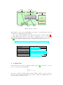
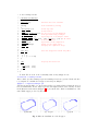
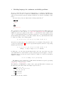
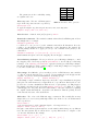
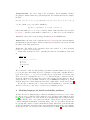
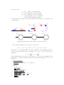
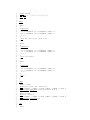
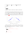
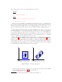
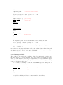
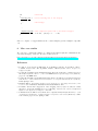
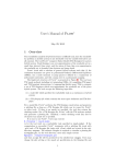
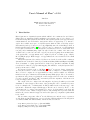
User’s Manual of Flow∗ v1.2.0
Xin Chen
RWTH Aachen University, Germany.
[email protected]
November 20, 2013
1
Introduction
Hybrid systems are dynamical systems which exhibit both continuous flow and discrete
jumps. They are natural modeling formalism for the systems composed of a discrete controller interacting with a physical environment. Since hybrid systems often appear in safetycritical situations, it is non-trivial to study their behavior. A typical way to do that is to
explore the reachable state space of a hybrid system, which is called reachability analysis.
Unfortunately, such a job can not be done algorithmically, since the reachability problem on
hybrid systems is undecidable [1]. The tool Flow∗ tries to compute an over-approximation
for a bounded reachable set of a hybrid system. A reachable set w.r.t. a bounded time horizon [0, T ] and a maximum jump depth k is called bounded, it consists of the states each
of which can be reached at some time t ∈ [0, T ] via at most k jumps from an initial state
of the system. The over-approximation set computed by Flow∗ is a finite group of Taylor
Model (TM) flowpipes. Each flowpipe over-approximates the exact reachable set in a small
time interval.
The hybrid system models considered by Flow∗ are described as follows. The continuous
dynamics in a mode should be defined by a non-linear Ordinary Differential Equation (ODE).
A mode invariant or a jump guard should be defined by polynomial constraints. A jump
reset should be defined by a polynomial mapping. The initial set of a hybrid system can be
given by an interval or a TM.
We present a birdview of the tool in Figure 1. Flow∗ accepts two classes of input files.
A model file describes a bounded reachability problem on a hybrid or continuous system.
The tool tries to compute an over-approximation for the bounded reachable set. A TM file
includes a state space definition as well as finitely many TM flowpipes. The tool reads those
specifications and generates a plotting file for the flowpipes. In both of the cases, an unsafe
set can be specified, and Flow∗ will conservatively check the emptiness of the intersection
between flowpipes and the unsafe set.
The output of Flow∗ consists of the following files. A plotting file which provides a 2D
visualization of the flowpipes. The format of the plotting file can be determined by users,
it can be a Gnuplot file or a Matlab file. A TM file which describes the state space of the
system and contains all computed TM flowpipes. The file can be reused by Flow∗ , or the
content may also be extracted and analyzed by other tools. If an unsafe set is given and
the tool detected some “unsafe” flowpipes, then a counterexample file is generated. The file
includes all potential unsafe flowpipes as well as the (discrete) computation paths which
lead to them.
The two main components of Flow∗ are the TM integrator and the image computation
module. In the module TM integrator, we provide three different schemes for the integration
of non-linear ODEs. The functionalities of them are listed as follows.
– Poly ODE 1 prefers low-degree polynomial ODEs.
– Poly ODE 2 prefers high-degree polynomial ODEs.
– Nonpoly ODE prefers non-polynomial ODEs.
TM file
Model file
TM parser
Model parser
TM arithmetic
TM integrator
Image Computation
Poly
Poly
Nonpoly
ODE 1
ODE 2
ODE
Domain
contraction
Range
over-approx.
TM analyzer
Plotting file
Result
TM file
Fig. 1. Structure of Flow∗
Although the low-degree polynomial ODEs are also supported by the last scheme, they can
be handled more efficiently by the first scheme.
Our tool has a simple installation. After that the libraries and tools listed in Table 1 are
properly installed, users only need to type make to compile the source code, and then an
executable file flowstar is generated. Most of the technical details of Flow∗ are described
in [2,3]. Please visit the following web page to fetch the current version of the tool.
http://ccis.colorado.edu/research/cyberphysical/taylormodels/
Names
GMP Library
GNU MPFR Library
GNU Scientific Library
GNU Linear Programming Kit
Bison - GNU parser generator
flex: The Fast Lexical Analyzer
Gnuplot
Weblinks
http://gmplib.org/
http://www.mpfr.org/
http://www.gnu.org/software/gsl/
http://www.gnu.org/software/glpk/
http://www.gnu.org/software/bison/
http://flex.sourceforge.net/
http://www.gnuplot.info/
Table 1. Libraries and tools used by Flow∗
2
A Quick Start
We start the usage of Flow∗ by a simple example given in [4]. A Van-der-Pol oscillator
can be modeled by the following ODE:
x˙ = y
y˙ = y − x − x2 · y
We want to compute the TM flowpipes from the initial condition x ∈ [1.25, 1.55], y ∈
[2.25, 2.35] in the bounded time horizon [0, 7]. Such a continuous reachability task can be
described by the following model file.
1
# file vanderpol.model
2
3
4
5
continuous reachability
{
state var x,y
# declare the state variables
6
7
8
9
10
11
12
13
14
15
16
17
18
19
setting
# the reachability setting
{
fixed steps 0.02
# time step size
time 7
# time horizon
remainder estimation 1e-5 # [-1e-5,1e-5] in each dimension
QR precondition
# the preconditioning technique
gnuplot octagon x,y
# plotting file is in Gnuplot format
adaptive orders { min {x:4 , y:4} , max {x:6 , y:6} } # TM orders
cutoff 1e-15
# cutoff threshold
precision 53
# precision in the computation
output vanderpol
# name for the output files
print on
# display the computation steps
}
20
21
22
23
24
25
poly ode 1
{
x’ = y
y’ = y - x - x^2*y
}
# use the integration scheme Poly ODE 1
26
27
28
29
30
31
32
init
{
x in [1.25 , 1.55]
y in [2.25 , 2.35]
}
}
# specify the initial set
To make Flow∗ work on the reachability task, we may simply execute
$./flowstar < vanderpol.model
After a while, two files vanderpol.plt and vanderpol.flow are generated in the subdirectory outputs. To visualize the flowpipes, users may use Gnuplot
$gnuplot < outputs/vanderpol.plt
and then an eps file will be produced in the subdirectory images. If the plotting file is specified as a Matlab file, then a .m file is generated in outputs, and it can be directly executed
in the Matlab environment. In Figure 2, we present the three kinds of visualizations of the
same TM flowpipes produced by Flow∗ .
(a) intervals
(b) octagons
Fig. 2. Different visualizations of the flowpipes
(c) grids
3
Modeling language for continuous reachability problems
We give a detailed introduction for the modeling language of continuous reachability problems in Flow∗ . To describe a continuous reachability task, we should first define the initial
value problem and then specify the parameters which are used in the reachability computation.
An initial value problem is defined in the following form in Flow∗ ,
poly ode 1
{
# ODE
}
init
{
# initial set
}
The option poly ode 1 tells the tool to use the integration scheme Poly ODE 1 and it can
be replaced by one of the other two, i.e., poly ode 2 and nonpoly ode. A d-dimensional
ODE can be given by d equations of the form x’ = ϕ such that x is a state variable and ϕ
can be a polynomial (in the first two integration schemes) or a non-polynomial expression
(in the last integration scheme) over the state variables. If ϕ is a polynomial then it should
be defined according to the following syntax
ϕ ::= ϕ + ϕ | ϕ - ϕ | ϕ * ϕ | -ϕ | (ϕ) | ϕ^n | x | r
wherein n is a positive integer, x is a variable and r is a real number. The priorities of the
operators are given in Table 2. If ϕ is a non-polynomial expression, then the corresponding
syntax is given as follows
ϕ ::= ϕ + ϕ | ϕ - ϕ | ϕ * ϕ | -ϕ | (ϕ) | ϕ^n | x | r
| sin(ϕ)
| cos(ϕ) | exp(ϕ) | ϕ / ϕ | sqrt(ϕ)
in which sin, cos are the trigonometric functions sine and cosine respectively, exp is the
exponential function, / is the division operator and sqrt denotes the square root. Flow∗
also allows users to specify time-varying disturbances which are bounded by intervals in
ODEs. For example,
x’ = 1 + 0.5*x*y - x^3 + [-0.01,0.01]
The initial set can be an interval or a TM. An interval initial set is given by specifying
each variable a single interval, for example
x in [1,2]
y in [-1,1]
The definition of a TM initial set consists of three parts: (1) TM variable declaration, (2)
the TM, and (3) the TM domain. An example is given as below,
tm var x0 , x1 , x2
x = 1 + x1^2 - x2 + [-0.02,0.01]
y = x0^3 - x1 + [0,0.1]
x0 in [-0.2,0.2]
x1 in [-0.2,0.2]
x2 in [-0.1,0.1]
wherein x,y are the state variables.
The parameters in the reachability setting
are explained as below.
operators priorities
^
4
- (prefix)
3
*
2
+
1
- (infix)
1
Time step size - The size of TM integration
Table 2. Priorities of the operators
steps. A fixed step size 0.02 can be specified by
fixed steps 0.02
To apply an adaptive step size ranges from 0.01 to 0.05, users may write
adaptive steps { min 0.01, max 0.05 }
Time horizon - A time horizon [0, T ] is given by time T.
Remainder estimation - The remainder estimation interval used in TM integration. Users
may simply write, for example
remainder estimation 1e-5
to tell Flow∗ to use [-1e-5,1e-5] as the estimation interval in all dimensions. It is also
possible to specify different remainder estimations over the dimensions. For example, the
following setting tells Flow∗ to apply [-2e-3,2e-3] to the x dimension and [-0.1,0.1] to the
y dimension.
remainder estimation { x:[-2e-3,2e-3], y:[-0.1,0.1] }
Small estimations help in control the wrapping effect in flowpipe construction.
Preconditioning technique - Flow∗ provides two preconditioning techniques to control
the wrapping effect. Users may specify QR precondition to use the QR preconditioning
technique, or use identity precondition to apply the identity preconditioning technique.
For the systems with more than 3 variables, QR preconditioning technique is not suggested
to use. More details can be found in [5].
Plot settings - It is difficult to plot even a 2D projection of a TM. Given two state variables
x, y, Flow∗ plots the interval (box) or octagon over-approximations of the flowpipes in the
x-y plane. To generate an interval visualization, users may specify
gnuplot interval x,y
or
matlab interval x,y
for the Gnuplot output or Matlab output respectively. For octagon visualization, users may
just replace the term interval by octagon in the above specification. Besides, Flow∗ also
provides more accurate visualizations which is based on grid pavings over TM flowpipes.
For example, users may use the plot setting gnuplot grid 10 x,y to tell Flow∗ to divide
a TM flowpipe into 10n parts, wherein n is the number of the state variables, by splitting
the original domain uniformly into 10 grids in each dimension. Then the plotting is based
on the interval enclosures of the subdivisions.
TM orders - The orders of the TMs in flowpipe construction. Theoretically, Flow∗ may
always achieve a better accuracy with higher TM orders. A fixed order 5 in all dimensions
can be specified as
fixed orders 5
or the user may want to apply a uniform adaptive order ranges from 3 to 6,
adaptive orders { min 3 , max 6 }
It is quite common that a system may have several variables which change at very different
rates. For such systems, Flow∗ allows users to specify different fixed or adaptive orders
over the state dimensions. For example,
fixed orders { x:3 , y:4 } or
adaptive orders { min { x:2 , y:3 } , max{ x:5 , y:4 } }
Cutoff threshold - In order to improve the performance, Flow∗ simplifies a TM by
sweeping the “small” terms in the polynomial part into the remainder interval. For example,
the TM
[0.5, 0.5] · x + [−1e − 5, −1e − 5] · y 2 + [0.1, 0.1] · x · y 2 + [5e − 4, 5e − 4] · x5 + [−1e − 3, 1e − 3]
over the domain x, y ∈ [−1, 1] will be simplified to
[0.5, 0.5] · x + [0.1, 0.1] · x · y 2 + [1.51e − 3, 1.51e − 3]
if the terms within [−1e − 3, 1e − 3] are considered “small”. Such a threshold can be specified
by cutoff ε, and then a term which is contained in [−ε, ε] will be moved to the remainder.
Precision - the precision of the floating-point numbers in the MPFR library.
Output name - the name of the output files. If output model is specified, then the Gnuplot
and Matlab plotting files will be named by model.plt and model.m respectively, the TM
file will be of the name model.flow.
Print out - The display of the computation steps can be turned on or off by specifying
print on or print off respectively.
Additionally, an unsafe set can be optionally given after the reachability problem, such
as
unsafe set
{
# polynomial constraints
p1 <= c1
p2 >= c2
p3 in [c3,c4]
...
}
The set should be defined by finitely many polynomial constraints. That is, the set is composed by the states that satisfy all of the constraints. A polynomial constraint should be
given as the form p ∼ c or p in [c1,c2] wherein p is a polynomial over the state variables, c,c1,c2 are constants and ∼∈ {<=, >=, =}. After the flowpipe construction, Flow∗
checks the emptiness of the intersection between the flowpipes and the unsafe set. If it is
empty, then the tool reports SAFE, otherwise it reports UNKNOWN and dumps the potential
unsafe flowpipes in a counterexample file the format of which will be described in Section 5.
For the sake of efficiency, the tool uses naive interval arithmetic to check the safety.
Therefore, it is better to give linear constraints in a reachability problem.
4
Modeling language for hybrid reachability problems
We introduce the modeling language for hybrid reachability problems by a concrete example. The model of a collision avoidance maneuver of two aircraft at a fixed altitude is given
in [6]. In the beginning, both of the aircraft are in straight flight with a relative heading.
When the aircraft come too close, that is, the distance of them is blow a specified value, the
controller will make an instantaneous heading change of 90◦ on both of them, and then the
two aircraft will complete a π-time semicircular arc flying. Afterwards, both aircraft make
another 90◦ instantaneous heading change and resume their headings in the very beginning.
Such a system can be modeled by a 3-mode hybrid system, see Figure 3. The state variables
are listed as below,
x1 , y1
α1 :
x2 , y2
α2 :
z:
: the coordinates of the first aircraft
the heading angle of the first aircraft
: the coordinates of the second aircraft
the heading angle of the second aircraft
timer for the semicircular arc flying
A heading angle is the angle between the heading direction and the vector (1, 0)T in the
coordinate map.
D
α1
α2
Mode 1
Mode 2
Mode 3
Fig. 3. Hybrid automaton of the collision avoidance maneuver
The continuous dynamics in each mode are of the form
x˙ 1 = v1 · cos α1 , y˙ 1 = v1 · sin α1 , x˙ 2 = v2 · cos α2 , y˙ 2 = v2 · sin α2
The angles α1 , α2 only changes in Mode 2, and so is the timer z. For the jump from Mode 1
to Mode 2, the guard is given by the constraint (x1 − x2 )2 + (y1 − y2 )2 ≤ D2 , and the reset
mapping is
π
π
α10 := α1 − , α20 := α2 −
2
2
For the jump from Mode 2 to Mode 3, the guard is z = π, and the reset mapping is same
as the above one. Our model file is shown as below wherein we simply choose v1 = v2 = 1
and D = 2.
1
2
3
hybrid reachability
{
state var x1, y1, alpha1, x2, y2, alpha2, z
4
5
6
7
8
9
10
11
12
13
14
setting
{
fixed steps 0.02
time 15
remainder estimation 1e-6
identity precondition
gnuplot octagon x1,y1
adaptive orders { min 2 , max 5 }
cutoff 1e-12
precision 53
output aircraft
max jumps 2
# bound of the jump depth
print on
15
16
17
18
}
19
20
21
22
23
24
25
26
27
28
29
30
31
modes
{
mode1
{
nonpoly ode
{
x1’ = cos(alpha1) y1’ = sin(alpha1) alpha1’ = 0
x2’ = cos(alpha2) y2’ = sin(alpha2) alpha2’ = 0
z’ = 0
}
inv { (x1 - x2)^2 + (y1 - y2)^2 >= 4 }
}
32
33
34
35
36
37
38
39
40
41
42
mode2
{
nonpoly ode
{
x1’ = cos(alpha1) y1’ = sin(alpha1)
x2’ = cos(alpha2) y2’ = sin(alpha2)
z’ = 1
}
inv { z <= 3.1415 }
}
alpha1’ = 1
alpha2’ = 1
mode3
{
nonpoly ode
{
x1’ = cos(alpha1)
x2’ = cos(alpha2)
z’ = 0
}
inv { }
}
alpha1’ = 0
alpha2’ = 0
43
44
45
46
47
48
49
50
51
52
53
54
y1’ = sin(alpha1)
y2’ = sin(alpha2)
}
55
56
57
58
59
60
61
jumps
{
mode1 - > mode2
guard { (x1 - x2)^2 + (y1 - y2)^2 = 4 }
reset { alpha1’ := alpha1 - 1.57075 alpha2’ := alpha2 - 1.57075 }
parallelotope aggregation { [x1:1,y1:1] [x2:1,y2:1] }
62
mode2 - > mode3
guard { z = 3.1415 }
reset { alpha1’ := alpha1 - 1.57075
parallelotope aggregation { }
63
64
65
66
67
}
68
69
70
71
init
{
mode1
alpha2’ := alpha2 - 1.57075 }
{
x1 in [-0.1,0.1]
x2 in [9.9,10.1]
z in [0,0]
}
72
73
74
75
76
77
78
y1 in [-0.1,0.1]
y2 in [-0.1,0.1]
alpha1 in [0.785374,0.785376]
alpha2 in [2.35612,2.35613]
}
}
79
80
81
82
83
84
85
unsafe
{
mode1
mode2
mode3
}
set
{ x1 - x2 <= 0.2
{ x1 - x2 <= 0.2
{ x1 - x2 <= 0.2
x1 - x2 >= -0.2
x1 - x2 >= -0.2
x1 - x2 >= -0.2
y1 - y2 <= 0.2
y1 - y2 <= 0.2
y1 - y2 <= 0.2
y1 - y2 >= -0.2 }
y1 - y2 >= -0.2 }
y1 - y2 >= -0.2 }
The reachability task considers all the possible initial positions in the region [−0.1, 0.1] ×
[−0.1, 0.1] for the first aircraft, and the initial positions in the region [9.9, 10.1] × [−0.1, 0.1]
for the second aircraft. The initial heading angle of the first aircraft is π4 and that of the
second aircraft is 43 π. There are at most two jumps in the hybrid automaton, so we bound
the jump depth by 2. We set the time horizon [0, 15] such that the two jumps will definitely
be executed in 15 time units. The octagon enclosures of the two aircraft trajectories are
presented in Figure 4. Flow∗ verifies that the two aircraft never got too close to each other.
(a) First aircraft
(b) Second aircraft
Fig. 4. Collision avoidance maneuver
Similar to the modeling file of a continuous reachability problem, the description of a
hybrid reachability problem is also composed by two parts, i.e., the setting for reachability
computation and the initial value problem on a hybrid system. The locations (modes) and
jumps of a hybrid system are declared in modes { ... } and jumps { ... } respectively.
A mode is defined by the form
name
# name of the mode
{
# can also be ‘poly ode 2’ or ‘nonpoly ode’
poly ode 1
{
# ODE in the mode
}
inv
{
# polynomial constraints
}
}
and a jump from mode m1 to mode m2 is defined by the form
m1 -> m2
guard
{
# polynomial constraints
}
reset
{
# polynomial reset mapping with uncertainties
}
... # aggregation setting
Flow∗ accepts polynomial reset mappings given in the form of x’ := p wherein x is a
state variable and p is a polynomial over the state variables. Additionally, users may also
include an interval uncertainty, that is a reset mapping may also be of the form x’ := p +
[a,b]. An unspecified variable will be associated with an identity mapping, that is x’ :=
x.
The flowpipe/guard intersection of a jump is usually a non-convex or even a set of
disjoint fragments. To avoid dealing with each of them in the consequent computation,
we over-approximate (or aggregate) the intersection sets by an order 1 TM (with zero
remainder interval) which can be viewed as an parallelotope. It is not hard to compute the
transformations between the TM and parallelotope representations, however, to determine
a proper orientation for the aggregation set is not easy.
For a d-dimensional parallelotope, its orientation can be determined by d linearly independent vectors1 , the set of which is called template. We give an example in Figure 5. The two
flowpipes can be over-approximated by a parallelotope with the template {(1, 0)T , (0, 1)T },
or the template {(1, 1)T , (1, −1)T }. It is obvious that the template plays an important role
in the aggregation accuracy. In Flow∗ , we provide the following options to select a template
for aggregating the flowpipe/guard intersections for a jump.
y
y
x
T
T
(a) template {(1, 0) , (0, 1) }
x
T
T
(b) template {(1, 1) , (1, −1) }
Fig. 5. Example of flowpipe aggregation
– Interval aggregation. Flow∗ computes a box enclosure for the flowpipe union, similar
to the example shown in Figure 5(a). The specification is
interval aggregation
1
They are also the linear independent facet normals of the parallelotope.
– General parallelotopic aggregation. Users may simply specify
parallelotope aggregation { }
to tell Flow∗ to automatically determine the template based on the invariants, guard,
flow directions and so on. It is also allowed to give some vectors which will be definitely
selected by the tool. For a 3-dimensional example, the following specification
parallelotope aggregation { [x:1,y:1] [z:2] }
tells the tool to choose (1, 1, 0)T and (0, 0, 2)T in determining the template, the remaining
ones will still be selected automatically. Since the vector lengths make no sense in the
template, Flow∗ always normalizes the vectors to the length 1.
To the best of our knowledge, there is no approach to find the best template for an aggregation job. Hence we will add more heuristics into Flow∗ in the future.
5
5.1
Formats of the output files
TM files
For a continuous reachability problem, the TM file generated by Flow∗ is of the following
format,
state var x, y, ...
gnuplot octagon x , y
unsafe set
{
...
}
output model
continuous flowpipes
{
tm var x0, y0, ...
...
}
# state variable declaration
# plot setting
# defined by polynomial constraints
# output name
# declare the variables used in TMs
# TM flowpipes
A TM flowpipe is represented as
{
x = p + [a,b]
...
local_t in [0,r]
x0
in [c,d]
...
}
# TM in every dimension
# domain of the TM
wherein local t is the local time variable of the TM. It ranges in a time step interval.
Notice that the TM variables are automatically named by the tool, thereby their names
have nothing to do with the state variable names.
For a hybrid reachability problem, the generated TM file is of the following form. The
flowpipes are kept according to the mode sequences visited in the computation.
state var x, y, ...
# state variable declaration
mode1
{
...
}
# specify the mode invariants
...
computation paths
# computation paths of modes
{
m1 (n1 , [a1,b1]) -> m2 (n2 , [a2,b2]) -> ... -> mk;
...
}
gnuplot octagon x , y
output model
# plot setting
# output name
unsafe set
{
...
}
hybrid flowpipes
{
mode1
{
tm var x0, y0, ...
...
}
# declare the variables used in TMs
# TM flowpipes
...
}
# other modes in the computation tree
The computation paths of modes are also dumped. As an example, the path
m1 (n1 , [a1,b1]) -> m2 (n2 , [a2,b2]) -> ... -> mk
denotes a mode sequence from m1 to mk in the reachability computation. A segment
mi (n , [a,b]) -> mj
means that there is a jump which is numbered by n from the mode mi to the mode mj such
that the execution time is included by the interval [a,b]. For a hybrid system, the jumps
are numbered by 1, 2, . . . in the order of their declarations.
5.2
Counterexample files
The tool Flow∗ also provides the possibility to dump all potential unsafe flowpipes. Since
the TM flowpipes are over-approximations of the exact reachable set segments, we are not
able to prove the unsafety by detecting a nonempty intersection between the TM flowpipes
and the unsafe set. However, we may dump those potential unsafe TM flowpipes and they
can be used in further analysis work.
For a continuous reachability problem, the unsafe TM flowpipes are dumped into a
counterexample file of the following form.
{
starting time t
{
...
}
# starting time of the flowpipe
# TM flowpipe
...
}
For a hybrid reachability problem, the counterexample file is as follows,
mk
{
starting time t
{
...
}
# mode name
# local starting time of the flowpipe
# TM flowpipe
...
computation path: # the computation path leads to the unsafe flowpipes
m1 (n1 , [a1,b1]) -> m2 (n2 , [a2,b2]) -> ... -> mk;
}
...
Since we compute over-approximations, the counterexamples generated might be superfluous.
6
More case studies
We collected a considerable number of continuous and hybrid system benchmarks in the
case study homepage of Flow∗ . It can be found as below.
http://systems.cs.colorado.edu/research/cyberphysical/taylormodels/casestudies/
References
1. R. Alur, C. Courcoubetis, N. Halbwachs, T. A. Henzinger, P.-H. Ho, X. Nicollin, A. Olivero,
J. Sifakis, and S. Yovine. The algorithmic analysis of hybrid systems. Theor. Comput. Sci.,
138(1):3–34, 1995.
´
2. X. Chen, E. Abrah´
am, and S. Sankaranarayanan. Taylor model flowpipe construction for nonlinear hybrid systems. In Proc. of the 33rd IEEE Real-Time Systems Symposium (RTSS’12),
pages 183–192. IEEE, 2012.
´
3. X. Chen, E. Abrah´
am, and S. Sankaranarayanan. Flow*: An analyzer for non-linear hybrid systems. In Proc. of the 25th International Conference on Computer Aided Verification (CAV’13),
LNCS. Springer, 2013.
4. Matthias Althoff. Reachability Analysis and its Application to the Safety Assessment of Autonomous Cars. PhD thesis, Technischen Universit¨
at M¨
unchen, 2010.
5. K. Makino and M. Berz. Suppression of the wrapping effect by taylor model-based verified
integrators: Long-term stabilization by preconditioning. International Journal of Differential
Equations and Applications, 10(4):353 – 384, 2005.
6. I. Mitchell and C. Tomlin. Level set methods for computation in hybrid systems. In Proc. of the
3rd International Workshop on Hybrid Systems: Computation and Control (HSCC’00), volume
1790 of LNCS, pages 310–323. Springer, 2000.