Download User Manual for the Monolith NT.115

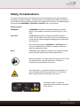
User Manual for the
Monolith NT.115
Table of Contents
Safety Considerations....................................................................................................... 4
Regulatory Statement ....................................................................................................... 7
Specifications ................................................................................................................... 8
Preface ........................................................................................................................... 10
Notices ........................................................................................................................... 10
Limited Warranty ............................................................................................................ 11
Installation Requirements ............................................................................................... 12
Installation and Connecting Cables................................................................................. 13
Maintenance and Operation............................................................................................ 14
Waste Treatment ............................................................................................................ 15
1. Introduction to Microscale Thermophoresis (MST) ...................................................... 16
1.1 Outline .................................................................................................................. 16
1.2 Method .................................................................................................................. 16
1.4 Selection of Recent Literature: .............................................................................. 19
2. Monolith NT.115 Instrument ........................................................................................ 20
2.1 Models .................................................................................................................. 20
2.2 Application Range ................................................................................................. 20
2.3 Sensitivity .............................................................................................................. 20
2.4 Sample Consumption ............................................................................................ 20
2.5 Capillary Format .................................................................................................... 21
2.6 Close-to-Native Conditions .................................................................................... 21
2.7 Dedicated NT Control Software and NT Analysis Software ................................... 21
3. Samples for MST ........................................................................................................ 22
3.1 Control Kit - Performing Standard Experiments ..................................................... 22
3.2 Selecting the Right Monolith NT™ Capillary .......................................................... 22
3.3 Checking the Sample Quality - Detecting Aggregation .......................................... 24
4. Preparing MST Experiments ....................................................................................... 26
5. Sample Loading .......................................................................................................... 29
2
6. Using the Monolith NT.115 Instrument ........................................................................ 31
7. NT Control Software ................................................................................................... 32
7.1 Temperature Control ............................................................................................. 33
7.2 Create New Projects or Load Existing Projects ..................................................... 34
7.3 Define Parameters for MST Measurements .......................................................... 35
7.4 Choose the LED Power for MST Measurements ................................................... 37
7.5 The Concentration Finder ...................................................................................... 38
7.6 Capillary Scan and MST Measurement ................................................................. 40
8. NT Analysis Software ................................................................................................. 42
8.1 NT Control Software - Update Mode and Load Function ....................................... 42
8.1.1 Update Mode - Loading MST Curves in Real Time ......................................... 42
8.1.2 Load Function - Loading Measurements from ntp-files ................................... 43
8.2 MST Data Analysis ................................................................................................ 44
8.2.1 “Thermophoresis with Jump”........................................................................... 45
8.2.2 ”Thermophoresis” ........................................................................................... 45
8.2.3 “Temperature Jump” ....................................................................................... 45
8.2.4 “Manual” ......................................................................................................... 46
8.3 Curve Fitting .......................................................................................................... 48
8.3.1 Kd Fitting ......................................................................................................... 48
8.3.2 Hill Fitting ........................................................................................................ 48
8.3.3 Data point removal.......................................................................................... 50
8.4 Save MST Data ..................................................................................................... 51
8.4.1 Save as Image File ......................................................................................... 51
8.4.2 Save as Text File ............................................................................................ 51
8.5 Generation of MST Report .................................................................................... 51
3
Safety Considerations
To ensure operation safety, this instrument must be operated correctly and maintained
according to a regular schedule. Carefully read to fully understand all safety precautions
in this manual before operating the instrument. Please take a moment to understand what
the signal words WARNING!, CAUTION and NOTE mean in this manual.
Safety symbols
WARNING!
A WARNING! indicates a potentially hazardous situation
which, if not avoided, could result in serious injury or even
death.
CAUTION
A CAUTION indicates a potentially hazardous situation
which, if not avoided, may result in minor or moderate injury.
It may also be used alert against damaging the equipment or
the instrument.
Do not proceed beyond a WARNING! or CAUTION notice
until you understand the hazardous conditions and have
taken the appropriate steps.
NOTE
A NOTE provides additional information to help the operator
achieve optimal instrument and assay performance.
Read manual label. This label indicates that you have to read
the manual before using the instrument. This label is
positioned at the backside of the device
Warning symbol. This symbol indicates laser radiation, it is
put on products which have a laser built in. This warning
label is positioned at the backside of the device.
Identification label. This label is
positioned at the backside / rear panel
of the device.
4
WARNING! Do only operate the Monolith NT.115 instrument with the delivered external
power supply (SPU63-105, Sinpro Electronic Co Ltd or Ael60US12, XP Power LLC or
GS90A12-P1M, MeanWell or GS60A12-P1J, MeanWell). Do only use the delivered
cables and plugs. If not doing so you risk electric shock and fire.
WARNING! Do not operate the Monolith NT.115 with substances and under conditions
which do cause a risk of explosion, implosion or release of gases. Only operate the
Monolith NT.115 with aqueous solutions.
CAUTION Ensure that the power plug of the external power supply is well accessible.
The Monolith NT.115 instrument has to be installed in a way that it does not hinder the
access to the external power supply and its power plug.
CAUTION The weight of the Monolith NT.115 instrument is approx. 24 kg, do not move
the instrument alone (two persons required for transport). If you move the instrument
alone it poses a risk of personal injury or damage to the instrument.
CAUTION The manual opening of the instrument is not allowed. Manual opening pose a
risk of personal injury or damage to the instrument. Contact NanoTemper service
personnel if you need to open the instrument.
CAUTION The instrument contains an IR-laser module (invisible laser radiation class 3B
according to IEC 60825-1: 2007). Lasers or laser systems emit intense, coherent
electromagnetic radiation that has the potential of causing irreparable damage to human
skin and eyes. The main hazard of laser radiation is direct or indirect exposure of the eye
to thermal radiation from the infrared B spectral regions (1,400 nm – 3,000 nm). Direct
eye contact can cause corneal burns, retinal burns, or both, and possible blindness. Do
not open the instrument while it is switched on. Manual opening of the instrument during
operation poses a risk of personal injury or damage to the instrument. When the
instrument is used as intended it emits laser radiation of LASER CLASS 1.
CAUTION Mechanical moving parts within the instrument can pinch or injure your hands
or fingers. Do not touch the instrument while parts are moving.
CAUTION The instrument contains a temperature regulator to control the sample
temperatures. Some accessible parts of the instrument can reach temperatures up to
50°C. Avoid touching the temperature controlled parts of the instrument for a longer time
when you have set the temperature controller to high temperatures.
CAUTION Only NanoTemper stuff is allowed for servicing and opening of the instrument.
Turn off the power switch and unplug the power cord before servicing the instrument,
unless otherwise noted. Connect the equipment only to the delivered power source. Do
not use extension cords. Have an electrician immediately replace any damaged cords,
plugs, or cables. Not doing so poses a risk of personal injury or damage to the
instrument.
5
CAUTION Only open the sample loading site, when moving parts in instrument are at
rest. Do not insert or remove a sample while linear actuator, laser or LED is at work.
Moving parts in the instrument can be harmful.
CAUTION Do not use the instrument in the cold room.
CAUTION Turn off the main circuit breaker in the back of the chassis, when the
instrument is not in use.
CAUTION Do not use ethanol or other types of organic solvents to clean the instrument
as they may remove the instrument paint.
CAUTION Use the instrument only for biomolecule analytics with aqueous solutions and
do not open the instrument on other site than for sample loading.
CAUTION Only use aqueous sample for analysis in the instrument.
CAUTION Do not use the instrument with hazardous substances or substances/materials
which pose a risk of infections.
6
Regulatory Statement
The following safety and electromagnetic standards were considered:
 IEC 61010-1:2001 Safety requirements for electrical equipment for measurement,
control and laboratory use. Part 1 General Requirements
 IEC 61010-2-010:2005 Safety requirements for electrical equipment for measurement,
control and laboratory use. Part 2-010: Particular requirements for laboratory
equipment for the heating of materials.
 IEC 61010-2-081:2001 Safety requirements for electrical equipment for measurement,
control and laboratory use. Part 2-081: Particular requirements for automatic and
semi-automatic laboratory equipment for analysis and other purposes.
 IEC 60825 Laser safety.
 IEC 61326-1:2006 EMC, Electrical equipment for measurement, control and laboratory
use – EMC requirements.
 IEC 61000-3-2:2006 EMC, Limits for harmonic current emissions (equipment input
current up to and including 16A per phase).
 IEC 61000-3-3:2008 EMC, Limits
7
Specifications
Input external power supply :90–264 VAC ± 10% 47–63 Hz, 230 VA max
Output external power supply: 12 VDC, 5.0 A max, 2.4 A typical
Electrical input Monolith NT.115 instrument: 12 VDC, 5A
Environmental
Operating temperature 15 – 30°C (Indoor use only)
Storage temperature -20 – 30°C
Humidity 0–80%, noncondensing
Operating altitude max 2000m
Monolith NT.115 Size
width 33 cm (13”)
height 45 cm (17.5”)
depth 51 cm (20”)
Weight 24 kg (51 lbs) net
Power supply size
width 10.6 cm (4.2”)
height 3 cm (1.2”)
depth 6.5 cm (2.6”)
Power supply Weight 0.23 kg (0.51 lbs) net max
IR laser
Wavelength: 1475 nm +/- 15 nm
Power: 120 mW max.
Monolith NT.115 Laser classification
Device is LASER PRODUCT CLASS 1
Temperature Control
Range: 22°C – 45°C (at Room Temperature 25°C)
Accuracy: +/- 0.3°C
Noise Level of Monolith NT.115 instrument:
max. 64 dB(A)
8
Connections
All ingoing and outgoing connections can be found at the rear panel of the instrument.
Name
Function
Ethernet
Connector for connecting the Ethernet cable to the PC/Notebook.
USB
Connector for connecting the USB cable to the PC/Notebook.
Only used for service by NanoTemper service.
Power Switch
When the switch is pressed on (position “I”), the instrument is
switched on.
DC Input
The connector to the external power supply. Connect with the
external power supply.
9
Preface
This manual is your guide for using the Monolith NT.115 and doing Microscale
Thermophoresis (MST) measurements. It instructs first-time users on how to use the
instrument, and serves as a reference for experienced users.
Before using the Monolith NT.115 instrument, please read this instruction manual
carefully, and make sure that the contents are fully understood. This manual should be
easily accessible to the operator at all times during instrument operation. When not using
the instrument, keep this manual in a safe place. If this manual becomes lost, order a
replacement from NanoTemper Technologies GmbH.
Notices
1.
2.
3.
4.
5.
6.
7.
NanoTemper shall not be held liable, either directly or indirectly, for any
consequential damage incurred as a result of product use.
Prohibitions on the use of NanoTemper software
 Copying software for other than backup
 Transfer or licensing of the right to use software to a third party
 Disclosure of confidential information regarding software
 Modification of software
 Use of software on multiple workstations, network terminals, or by other
methods
The contents of this manual are subject to change without notice for product
improvement.
This manual is considered complete and accurate at publication.
This manual does not guarantee the validity of any patent rights or other rights.
If a NanoTemper software program has failed causing an error or improper operation,
this may be caused by a conflict from another program operating on the Notebook
(PC). In this case, take corrective action by uninstalling the conflict product(s).
NanoTemper is a registered trademark of NanoTemper Technologies GmbH in
Germany and other countries.
10
Limited Warranty
Products sold by NanoTemper, unless otherwise specified, are warranted for a period of
one year from the date of shipment to be free of defects in materials and workmanship. If
any defects in the product are found during this warranty period, NanoTemper will repair
or replace the defective part(s) or product free of charge.
THIS WARRANTY DOES NOT APPLY TO DEFECTS RESULTING FROM THE
FOLLOWING:
1. IMPROPER OR INADEQUATE INSTALLATION.
2. IMPROPER OR INADEQUATE OPERATION, MAINTENANCE, ADJUSTMENT OR
CALIBRATION.
3. UNAUTHORIZED MODIFICATION OR MISUSE.
4. USE OF UNAUTHORIZED CAPILLARIES AND CAPILLARY TRAYS.
5. USE OF CONSUMABLES, DISPOSABLES AND PARTS NOT SUPPLIED BY AN
AUTHORIZED NANOTEMPER DISTRIBUTOR.
6. CORROSION DUE TO THE USE OF IMPROPER SOLVENTS, SAMPLES, OR DUE TO
SURROUNDING GASES.
7. ACCIDENTS BEYOND NANOTEMPER’S CONTROL, INCLUDING NATURAL
DISASTERS.
This warranty does not cover consumables like capillaries, reagents, labeling kits, and the
like.
The warranty for all parts supplied and repairs provided under this warranty expires on
the warranty expiration date of the original product. For inquiries concerning repair
service, contact NanoTemper after confirming the model name and serial number of your
NanoTemper instrument.
11
Installation Requirements
To ensure operation safety, observe the following conditions:
1.
2.
3.
4.
5.
6.
7.
8.
9.
10.
11.
12.
13.
14.
15.
16.
17.
18.
Do only operate the Monolith NT.115 instrument with the delivered external power
supply (SPU63-105, Sinpro Electronic Co Ltd or Ael60US12, XP Power LLC or
GS90A12-P1M, MeanWell or GS60A12-P1J, MeanWell).
Only connect the external power supply of Monolith NT.115 to an electrical socket
containing a protective conductor terminal.
Ensure that the power plug of the external power supply is well accessible. The
Monolith NT.115 instrument has to be installed in a way that it does not hinder the
access to the external power supply and its power plug.
Only operate the instrument with the delivered PC (Notebook).
Only operate the instrument with original Monolith NT.115 capillary trays.
The maximum noise level of the instrument is 64 dB(A). Only operate the instrument
in an environment where this noise level is appropriate.
Operate the instrument in a temperature range of 15 – 30°C.
Operate the instrument in a humidity range of 0 – 80 % (RH). If ambient humidity
exceeds 80 % (RH), condensation may deteriorate optical components.
Operate the instrument in an atmospheric pressure range of 800 – 1060 hPa.
Do not operate the Monolith NT.115 under conditions which pose a risk of explosion,
implosion or the risk of the release of gases.
Avoid strong magnetic fields and sources of high frequency. The instrument may not
function properly when near a strong magnetic field or high frequency source.
Avoid vibrations from vacuum pumps, centrifuges, electric motors, processing
equipment and machine tools.
Avoid dust and corrosive gas. Do not install the instrument where it may by exposed
to dust, especially in locations exposed to outside air or ventilation outlets.
For cleaning the instrument, only use water.
Do not install the instrument in a location where it may be exposed to direct sunlight.
Install the instrument in a horizontal and stable position. (This includes a table, bench
or desk upon which the instrument is installed).
Ensure that no air conditioner blows air directly onto the instrument. This may
prevent stable measurements.
Install the instrument in a location that allows easy access for maintenance.
NOTE: The above conditions do not guarantee optimal performance of this instrument.
12
Installation and Connecting Cables
Preparation
Prepare a table which can bear a weight of about 50 kg and has a free area of 80 cm
(width) x 50 cm (depth).
Put the Monolith NT.115 instrument and the Notebook to this free area.
CAUTION The weight of the Monolith NT.115 instrument is approx. 24 kg, do not move
the instrument alone (two persons required for transport/movement). If you move the
instrument alone it poses a risk of personal injury or damage to the instrument.
Connecting the Power supply and the Monolith NT.115
Confirm that the power switch of the Monolith NT.115 instrument is off (power switch is at
the backside, left of the instrument).
WARNING! Do only operate the Monolith NT.115 instrument with the delivered external
power supply (SPU63-105, Sinpro Electronic Co Ltd or Ael60US12, XP Power LLC or
GS90A12-P1M, MeanWell or GS60A12-P1J, MeanWell). Do only use the delivered
cables and plugs. If not doing so you risk electric shock and fire.
Connect the external power supply to the electrical socket. Then connect the power
supply to the Monolith NT.115 instrument.
CAUTION Ensure that the power plug of the external power supply is well accessible.
The Monolith NT.115 instrument has to be installed in a way that it does not hinder the
access to the external power supply and its power plug.
Connect the Monolith NT.115 instrument to the Notebook by using the delivered network
cable.
Switch on the Monolith NT.115 and the Notebook.
13
Maintenance and Operation
Pay attention to the instrument operating environment and always keep it clean so that
the instrument can be used in a stabilized condition over a long period. Do not place
anything on the instrument.
Cleaning the Monolith NT.115 instrument
Switch off the instrument and remove the power plug of the external power supply from
the electrical socket. Only use dry cloth or cloth wetted with water for cleaning of the
instrument.
CAUTION Do not use ethanol or other types of organic solvents to clean the instrument
as they may remove the instrument paint.
Transporting the Monolith NT.115 instrument
Switch off the instrument and remove the power plug of the external power supply from
the electrical socket. Do not carry the instrument alone, two people are need for
transportation.
CAUTION The weight of the Monolith NT.115 instrument is approx. 24 kg, do not move
the instrument alone (two persons required for transport/movement). If you move the
instrument alone it poses a risk of personal injury or damage to the instrument.
Functional Disorder
In case of a functional disorder switch off the Monolith NT.115 instrument and wait for five
minutes, then switch on the instrument again. If there is still a functional disorder switch
off the device, unplug the power cable and contact the NanoTemper service.
Repairing the Monolith NT.115 instrument
Do not try to repair the instrument by yourself. Do contact the NanoTemper service for
repairing the instrument.
CAUTION The manual opening of the instrument is not allowed. Manual opening pose a
risk of personal injury or damage to the instrument. Contact NanoTemper service
personnel if you need to open the instrument.
14
Waste Treatment
Waste treatment is your own responsibility. You must hand it to a company specialized in
waste recovery. Do not dispose the instrument in a litter bin or at a public waste
disposable site. For detailed information please contact the NanoTemper service. 1.
Introduction to Microscale Thermophoresis (MST)
15
1. Introduction to Microscale Thermophoresis
(MST)
1.1 Outline
Microscale Thermophoresis (MST) is based on a physical principle used for the first time
in bioanalytics. It detects changes in the hydration shell, charge or size of molecules by
measuring changes of the mobility of molecules in microscopic temperature gradients. It
allows fast detection of a wide range of biomolecular interactions from ion or fragment
binding up to interactions of large complexes (e.g. liposomes and ribosomes). The main
key feature of MST is the possibility to work under close-to-native conditions:
Measurements are performed immobilization-free and in any buffer or complex bioliquid
(e.g. serum and cell lysate). Other key features comprise easy sample preparation, low
sample consumption of less than 4 μl per sample at nM concentration and a high
dynamic range of dissociation constants between sub-nM to mM. Furthermore the
Monolith NT.115TM is maintenance-free, has low running costs and uses an intuitive
software user interface.
1.2 Method
The measurement method is based on the directed movement of molecules along a
temperature gradient, an effect termed “thermophoresis”. A local temperature difference
ΔT leads to a local change in molecule concentration (depletion or enrichment),
quantified by the Soret coefficient ST: chot/ccold=exp(-STΔT).
Thermophoresis depends on changes in size, charge and solvation shell of molecules.
We monitor the thermophoresis of fluorescent molecules in titration experiments where
the buffer is always kept constant. As the buffer is kept constant, alterations in the
thermophoretic depletion or enrichment can only arise from changes in the size, charge
or solvation entropy of the fluorescent molecules. As the binding of a titrated, nonfluorescent molecule to a labeled molecule changes at least one of these properties, the
binding can be quantified by measuring the change in thermophoresis.
16
Figure 1: Thermophoresis assay: (left) The solution inside the capillary is locally heated with a
focused IR-laser, which is coupled into the path of light using a hot mirror. (right) The fluorescence
inside the capillary is imaged with a photodiode and the normalized fluorescence in the heated
spot is plotted against time. The IR-laser is switched on at t=5s. The fluorescence decreases as
the temperature increases and the fluorescent molecules that formed complexes move away from
the heated spot due to thermophoresis.
The thermophoretic movement of the fluorescent molecule is measured by monitoring the
fluorescence distribution F inside a capillary with the NanoTemper Monolith instrument
(Figure 1, left). The microscopic temperature gradient is generated by an IR-Laser, which
is focused into the capillary and is strongly absorbed by water. The temperature of the
aqueous solution inside the laser spot is raised by 2K-6K compared to the periphery and
is thus creating a strong temperature gradient. Before the IR-Laser is switched on a
homogenous molecule distribution is observed inside the capillary. When the IR-Laser is
switched on, two effects, separated by their time-scales, are observed. As a first
response the fluorescence of the dye changes because of its intrinsic temperature
dependence. As a second response the molecules move from the locally heated region to
the outer cold regions and thus the concentration of molecules in the locally heated
region decreases until it reaches a steady state on a time scale of about 10s-30s which is
determined by mass diffusion. (Figure 1, right).
While the mass diffusion D dictates the kinetics of depletion, ST determines the steady
state concentration ratio chot/ccold=exp(-STΔT)≈1-(STΔT) under a temperature increase ΔT.
The normalized fluorescence Fnorm measures mainly this concentration ratio, plus a
temperature dependence of the dye. In the linear approximation we expect
Fnorm=Fhot/Fcold=1-(ST -dF/dT) ΔT. Within the titration experiment Fnorm changes according
to:
Fnorm=(1-x)F(A)norm + x F(AT)norm
(1)
Where F(A)norm is the contribution of the unbound fluorescent molecule A and F(AT)norm
the contribution of the complex of the fluorescent molecule A and its interacting titrant T
and x the fraction of fluorescent molecules that formed the complex. By increasing the
concentration of the non-labeled titrant and mixing it with a constant concentration of
17
fluorescent molecule, the fraction of complexes increases until all fluorescent molecules
formed complexes with the titrant. Thus the fraction of bound molecules x can be derived
from the measured change in normalized fluorescence Fnorm.
Figure 2: DNA-aptamer binding to Thrombin. (a) The thermophoretic movement of the unbound
aptamers differs from the movement of aptamers bound to thrombin. (b) The normalized
fluorescence signal of the DNA-aptamer at t=30s is plotted for different concentrations of thrombin
to result in a binding curve used for Kd fitting (see section below). As a negative control single
strand DNA (ssDNA, blue circles) was chosen. Here no changes in normalized fluorescence signal
with increasing thrombin concentration were obtained.
As an example the binding of a labeled DNA-aptamer to thrombin is shown in Figure 2. In
this example the concentration of labeled aptamer is kept constant and the thrombin
concentration is titrated. Plotting Fnorm against the concentration of thrombin results in a
binding curve from which the dissociation constant Kd can be derived (Figure 2b).
The dissociation constant Kd is obtained by fitting the binding curve with the quadratic
solution for the fraction of fluorescent molecules that formed the complex, calculated from
the law of mass action. The definition of the dissociation constant is Kd=[A]*[T]/[AT] where
[A] is the concentration of free fluorescent molecule, [T] the concentration of free titrant
and [AT] is the concentration of complexes of [A] and [T]. The free concentrations of A
and T are [A]=[A0]-[AT] and [T]=[T0]-[AT], respectively. [A0] is the known concentration of
the fluorescent molecule and [T0] is the known concentration of added titrant. This leads
to a quadratic fitting function for [AT]:
[AT]=1/2*(([A0]+[T0]+ Kd)-(([A0]+[T0]+ Kd)2-4*[A0]*[T0])1/2)
(2)
The concentration of fluorescent molecule [A0] is kept constant during the experiments
and the concentration of titrant [T0] is varied by titration. The signal obtained in the
measurement (equation 1) directly corresponds to the fraction of fluorescent molecules
that formed the complex x=[AT]/[A0] which can be easily fitted with the derived formula to
obtain Kd. In the results section of this report the relative fluorescence Fnorm is plotted in
‰.
18
1.4 Selection of Recent Literature:
Wienken et al., Nature Communications (2010),
Protein Binding Assays in Biological Liquids using Microscale Thermophoresis.
Jerabek-Willemsen et al., ASSAY and Drug Development Technologies (2011),
Molecular Interaction Studies Using Microscale Thermophoresis.
van den Bogaart et al., JBC (2012),
Phosphatidylinositol 4,5-bisphosphate increases the Ca2+ affinity of synaptotagmin-1 40-fold.
Lin et al., Cell (2012),
Inhibition of Basal FGF Receptor Signaling by Dimeric Grb2.
Seidel et al., Angewandte Chemie (2012),
Label-Free Microscale Thermophoresis Discriminates Sites and Affinity of Protein–Ligand Binding
Seidel et al., Methods (2013),
Microscale thermophoresis quantifies biomolecular interactions under previously challenging
conditions.
19
2. Monolith NT.115 Instrument
2.1 Models
Monolith
Instrument
LED
1
LED
2
Blue Dyes
Green Dyes
Red Dyes
NT.115
Blue/Green
FITC/FAM/GFP/
YFP
Cy3/RFP/mCherry
no detection
NT.115
Blue/Red
FITC/FAM/GFP/
YFP
no detection
Cy5/Alexa647
NT.115
Green/Red
YFP
Cy3/RFP
Cy5/Alexa647
2.2 Application Range
The Monolith NT.115 allows to measure the binding of all kinds of biomolecules (Kd = 1
nM – 500 mM) as well as the activity of enzymes. Higher Affinities are accessible in
competition experiments.
2.3 Sensitivity
The Monolith NT.115 can measure as little as the binding of single ions (40 Da) or small
molecules (300 Da) to a target as well as the binding of large complexes such as
ribosomes (2.5 MDa).
2.4 Sample Consumption
The Monolith NT.115 requires only little sample material: >1 nM of the labeled compound
and a titration of the unlabelled compound in the range of ± factor 10- to 20-fold of the
expected dissociation constant. For standard applications, 4 μl of sample material is filled
in the capillary.
20
2.5 Capillary Format
The capillary format used for the Monolith NT.115 is inexpensive, easy to handle and
offers a maximum of flexibility in the experiment scale. The standard sample tray format
allows to process automatically up to 16 capillaries (e.g. for a detailed Kd-analysis), or
alternatively to perform smaller pilot experiments involving only 2-3 sample
concentrations.
2.6 Close-to-Native Conditions
The Monolith NT.115 can monitor the binding and the biochemical activity of
biomolecules under close-to-native conditions:
-
immobilization-free
In a solution of choice, ranging from standard and proprietary buffers to complex
bioliquids including blood serum, cell lysates, and the like
2.7 Dedicated NT Control Software and NT Analysis Software
The Monolith NT.115 is supported by software for instrument control and analysis. For
more detailed information see chapter 7 und 8.
21
3. Samples for MST
For detailed information about handling capillaries please read chapter 5.
3.1 Control Kit - Performing Standard Experiments
Control Kits containing standardized sample material are recommended
-
when using the Monolith NT.115 instrument for the first time
for monitoring the correct performance of the Monolith NT.115
for training of new lab employees
Optimized Control Kits for use in Microscale Thermophoresis are available either with
red- or green-fluorescently labeled biomolecules.
The kits contain a fluorescent-labeled DNA-molecule, unlabeled binding partner and
buffer.
Cat #
C030
C031
Monolith Control Kits
Monolith NT™ Control Kit RED Molecular Interaction Control
Kit for Monolith NT.115 BLUE/RED or Monolith NT.115
GREEN/RED
Monolith NT™ Control Kit GREEN Molecular Interaction
Control Kit for Monolith NT.115 BLUE/GREEN or Monolith
NT.115 GREEN/RED
Reactions
5
5
3.2 Selecting the Right Monolith NT™ Capillary
In order to avoid experimental artifacts, which can be caused by protein adsorbance to
the glass capillary or by protein aggregations, it is recommended to determine the best
Monolith NT™ Capillary type for a biomolecule of interest by performing the following
experiment:
-
-
Load 4 Monolith NT™ Standard Treated Capillaries with 100 nM (or with working
concentration) of the labeled biomolecule of interest after diluting it with the buffer
that is intended to be used in the experiment.
Place the capillary on the tray and insert the tray in the instrument.
Chose a folder where to save the scan data and a LED color/power.
Close the front door and start a capillary scan by pushing the button “Start Cap
Scan”.
If a “U-shape” (i.e. split peak) is observed, instead of a distinct fluorescence peak, it
shows that your sample absorbs to the capillary wall. See figure below (left 3 capillaries):
22
sticking sample
false capillary
non-sticking sample
right capillary
NOTE: If you observe asymmetry or shoulders in the fluorescence peak repeat the
Capillary Scan 5-15 minutes after loading the capillaries.
or

In this case it is recommended to use Monolith NT™ Hydrophobic and Hydrophilic
Capillaries which in almost all cases prevent the absorbance to the capillary glass walls.
Cat #
D001
Monolith NT™ Capillaries
NT.115™ Capillary
Selection Set
K002
Monolith NT.115™
Standard Treated
Capillaries
Monolith NT.115™
Hydrophobic Capillaries
Monolith NT.115™
Hydrophilic Capillaries
K003
K004
Content
25 Monolith NT.115™ Standard Treated
Capillaries
25 Monolith NT.115™ Hydrophobic Capillaries
25 Monolith NT.115™ Hydrophilic Capillaries
1000 Capillaries
200 Capillaries
200 Capillaries
NOTE: Random variations of fluorescence counts can also be caused by
adsorption of the biomolecule to the micro reaction tubes. In this case, a
detergent or passivating agents like BSA may be used, a higher sample
volume may be prepared or low adsorption micro reaction tubes may be
deployed.
23
3.3 Checking the Sample Quality - Detecting Aggregation
In addition, the potential aggregation behavior of the biomolecule of interest can be tested
with Microscale Thermophoresis. Often protein preparations contain aggregates that are
very difficult to observe with standard methods. To test for the quality of your preparation
perform the following experiment with your molecule of interest at working concentration
and in the intended buffer:
Start a measurement with the following setting:
-
LED power adjusted to your sample concentration
MST power 40 %
MST power on time 30 seconds
MST power off time 5 seconds
In case that the biomolecule of choice aggregates, the fluorescence signal during the
“laser on time” is “bumpy” (examples see next page). This is because aggregates are
transported into the measurement volume by a convective flow induced by local heating.
Therefore always centrifuge your samples and any stock before using it in a MST
experiment (5 minutes, 13000 rpm, 4°C). You may also use detergents such as Tween 20
(0,01 % - 0,1 %) or Triton X-100 (0,01 % - 0,1 %).
24
No Aggregates
Some Aggregates – better sample preparation needed
Many Large Aggregates – better sample preparation needed
25
4. Preparing MST Experiments
For performing a molecular interaction experiment and measuring the dissociation
constant (Kd), a titration series of up to 16 dilutions is prepared, where the concentration
of the fluorescent binding partner is kept constant and the concentration of the unlabeled
binding partner is varied. Do not use less than 10 capillaries.
NOTE: Also competition experiments can be performed to analyze interactions.
E.g. a complex between two proteins is formed, one of them fluorescently
labeled. The concentration of this complex is kept constant, and a small
molecule or any other competitor is titrated to this complex. When the small
molecule is capable of separating the proteins, it is observed in
thermophoresis. Thus a functional assay is performed.
A) Prepare the labeled binding partner:
Ideally the ratio of fluorescence label to protein (DEG, degree of labeling) is 1:1 or less.
Non-bound fluorescence label has to be eliminated from the labeling mixture, completely.
The concentration of the protein should be smaller than or close to the expected Kd and
should yield between 100-1500 fluorescence counts (typically equivalent to 1-200 nM)
when measured with the Monolith NT.115.
The following kits offer optimized fluorescence labeling and purification protocols for use
in Microscale Thermophoresis. The dyes are widely tested with thermophoresis and the
protocols are optimized to remove free, non-reacted dye:
Cat #
L001
L002
L003
L004
L005
L006
Monolith NT™ Protein Labeling Kits
Monolith NT™ Protein Labeling Kit
RED-NHS (Amine Reactive)
Monolith NT™ Protein Labeling Kit
GREEN-NHS (Amine Reactive)
Monolith NT™ Protein Labeling Kit
BLUE-NHS (Amine Reactive)
Monolith NT™ Protein Labeling Kit
RED-MALEIMIDE (Cysteine Reactive)
Monolith NT™ Protein Labeling Kit
GREEN-MALEIMIDE (Cysteine Reactive)
Monolith NT™ Protein Labeling Kit
BLUE-MALEIMIDE (Cysteine Reactive)
Reactions
4x 100 µg protein
4x 100 µg protein
4x 100 µg protein
4x 100 µg protein
4x 100 µg protein
4x 100 µg protein
26
B) Prepare the unlabeled binding partner
Prepare a 16 step dilution series around the expected Kd, starting from a concentration of
20 fold the expected Kd, down to 0.02 fold the expected Kd. Prepare the samples with a
double concentration, since mixing volume ratio of 1:1 decreases the concentration by a
factor of 2.
Use sufficiently small micro reaction tubes to avoid evaporation of the sample (e.g. with a
volume < 100 µl when preparing 10-20 µl of sample).
Example: Interaction of protein X and compound Y. Kd = 50 nM.
Serial dilution: from 1000 nM to 0.025 nM
Compound Y stock: 1 mM in buffer YB
I.
II.
III.
IV.
V.
VI.
VII.
Prepare the highest concentration of the dilution series by diluting
compound Y to 2 µM in assay buffer (tube 1). This dilution still
contains traces of buffer YB.
Before starting the serial dilution of compound Y adjust the
composition of the assay buffer in order to obtain same
composition that is achieved in the first dilution (e.g. DMSO,
Glycerol, etc).
Prepare 15 tubes with 15 µl of the adapted assay buffer.
Then transfer 15 µl with a clean tip from tube 1 (2 µM compound Y
from step I) to tube 2 and mix well by pipetting.
With a clean tip transfer 15 µl from tube 2 to tube 3 and mix well.
Continue this serial dilution until tube 16.
Transfer 10 µl from tube 1 - 16 in new reaction tubes and add
10 µl of your fluorescently labeled sample e.g. 100 nM to the
tubes.
Mix very well by pipetting up and down to obtain good results.
Dilution
Series
1
2
3
4
5
6
7
8
9
10
11
12
13
14
15
16
Compound
Y (nM)
1000
500
250
125
62.5
31.2
15.5
7.7
3.7
1.8
0.90
0.45
0.22
0.11
0.05
0.025
C) Binding reaction
After preparing the serial dilution of the non-labeled binding partner, fill 10 μl of each step
of the dilution series into 16 fresh small micro reaction tubes. Afterwards fill 10 μl of a 2
fold stock solution of the labeled binding partner into the same 16 tubes and mix very well
by pipetting up and down. Incubate the samples in the dark. Incubation time and
temperature can differ between different molecules and should be tested in a pilot
experiment by the researcher. In most cases 5 minutes incubation at room temperature
are sufficient.
D) Transfer the binding reaction into Monolith NT™ Capillaries:
After the adequate incubation time samples from all 16 tubes are aspirated into Monolith
NT™ Capillaries (see chapter 5).
27
NOTE: When preparing the interaction partners, consider the following rules.
1. Centrifuge stock solutions before further usage to remove aggregates.
2. When the highest concentration of binder has a significant concentration
of an additional buffer component (e.g. 3 % DMSO), then the buffer used
for dilution has to contain the additive in same concentration. The same
holds true for differences in ionic strength or pH, BSA or glycerol
content.
3. The Monolith NT.115 has highly precise fluorescence detection and
insufficiently mixed samples will be highlighted by random fluctuating
fluorescence intensity signals. If sample are well mixed, a random
fluctuation of 10 % or even less is achieved.
4. In order to avoid bubbles or droplets etc. we recommend to carefully
pipett up and down several times and not to vortex these small volumes,
that may also lead to denatured protein or sample.
28
5. Sample Loading
Be careful when using the glass capillaries. Broken capillaries are harmful to skin and
eyes. Discard the capillaries only in waste boxes that are intended for use of glass waste.
Glass capillaries are not intended for use with infectious samples.
Wear gloves, safety glasses and lab coat.
Stick the Monolith NT™ Capillary horizontally into the reaction tube to aspirate the sample.
Don’t touch the capillary in the middle where the optical measurement will be performed.
Position the liquid in center of the Monolith NT™ Capillary, by holding it vertically and
shake it after aspirating the sample. Leave some air at both ends of the capillary.
29
Put the capillaries in the slots on the sample tray. Note the order of the capillaries. The
highest concentration is placed in the front of the tray. This position is denoted as “1” in
the sample tray and in the NT Control Software.
Place the sample tray in the instrument by pushing it into the tray slot of the instrument as
far as possible. The Monolith NT.115 instrument scans the tray and automatically
determines the position of the capillaries on the tray.
30
6. Using the Monolith NT.115 Instrument
First, start the MonolithTM NT.115 instrument at the back side and the control notebook.
The display of the MonolithTM NT.115 instrument will show the following picture:
The words “Ready” in the first line and “Connected” in the last line indicate the successful
connection between the MonolithTM NT.115 instrument and the control notebook.
The arrowheads on the right hand side (up and down) are used to open and to close the
front door of the instrument in order to load/remove the sample tray.
The activities of the instrument are shown in green letters “MST POWER OFF” and “LED
OFF”. As soon as an experiment is running these letters turn red and indicate “MST
POWER ON” and “LED ON”, respectively. The status of the LED informs you if
fluorescence detection is running and the status of the MST power if the IR laser is
working and generating temperature gradients in your samples.
In the middle of the screen you find information on the “Temperature Control”. First of all
you can see if the “Temperature Control” is activated (“OFF” or “ON”) – this is possible
with the NT Control Software (for details see next chapter). Below that you find
information on the “Actual Temperature” and the “Target Temperature” of the instrument.
Please note that this is not the laser induced temperature gradient used for MST
measurements.
For most measurements the room temperature is sufficient, so there is no adjustment
necessary.
IMPORTANT! Before running measurements, insert the tray containing capillaries
filled with your samples and wait for the “Target Temperature” to be reached!
To start a measurement, start the NT Control Software (for details see next chapter).
31
7. NT Control Software
With the NT Control Software interface all necessary parameters for the MonolithTM
NT.115 instrument can be set. It does not matter if you switch on the MonolithTM NT.115
instrument or the NT Control Software first. After starting the NT Control Software from
the desktop, the following screen appears:
Highlighted in red you see the connection between the MonolithTM NT.115 instrument and
the Monolith NT Control Software.
32
7.1 Temperature Control
For using the “Temperature Control” select the “Temperature Control” tool in the upper
menu bar and choose the function “Enable Manual Temperature Control”. Afterwards
type in the target temperature that you want to achieve in the instrument in the “Manual
Temperature Control” box and click “On”. Please note that this is not the laser induced
temperature gradient used for MST measurements. It adjusts the overall instrument
temperature.
Now you can also see on the screen of Monolith NT.115TM instrument that the
“Temperature Control” is activated “ON”. Further the display reports the “Actual
Temperature” and the “Target Temperature”. Please wait until the “Target Temperature”
is reached (usually less than 5 minutes).
IMPORTANT! Before running measurements, insert the tray containing capillaries
filled with your samples and wait for the “Target Temperature” to be reached!
IMPORTANT! Before closing the Monolith NT Control Software and switching off
the MonolithTM NT.115 instrument stop the “Manual Temperature Control” by
clicking “OFF” in the “Manual Temperature Control” box.
33
7.2 Create New Projects or Load Existing Projects
Before starting MST measurements one has to select a file where to save the data.
Therefore select the “File” option in the upper menu bar and choose the function “New
Project” or “Load Project”.
A new window will open in which you select storage medium and file name of your new or
an existing ntp-file. Verify by clicking “Save”. A ntp-file contains several MST experiments
that are listed accordingly to their name and the date & time when they were recorded. A
MST experiment can contain several runs that are listed accordingly to the “Table of
Runs” that you defined for your assay (e.g. different MST powers).
Afterward creating or opening a ntp-file give a name to the MST experiment that you want
to start in the “Actual Experiment`s Name” box.
34
7.3 Define Parameters for MST Measurements
Before starting your MST experiment you have to define the parameters for the MST
measurements. Therefore perform the following steps:
1. Select the “LED Color” fitting the dye that you are using in the box “LED Settings”.
LED Color
blue
green
red
Optimal excitation of
FITC, FAM, GFP, YFP, Alexa488 and similar
Cy3, RFP, mCherry, HEX and similar
Cy5, Alexa647, Dy647 and similar
2. Select the number of capillaries that you want to use in your measurement in the
box “Capillary Scanning”.
3. Also select the “LED Power” that you want to use or test in the same box
“Capillary Scanning”. The “LED Power” can be varied up to 100 %. How to choose
the best “LED Power” is described in the next chapter.
4. The next step is entering the concentrations of the serial dilution of your titrant
(unlabeled interaction partner) in the “Table of Capillaries”. How to choose the
concentration range best is described in one of the next chapters.
a. Therefore choose first the “Dilution” you are using e.g. 1:1.
b. Type in the highest concentration of the titrant in capillary “N° 01”. This is
the first capillary in the tray from the operator´s point of view.
c. Then after entering the first concentration, move while holding the left
mouse button to the concentrations field below. The serial dilution of the
concentration will be calculated automatically. Please use only numbers in
the column “Concentration”.
d. The column “Name” accepts both numbers and letters. You can add
information in this column like “micromolar AMP” etc…
5. The table of runs describes the parameters of the MST measurements that are
performed. The “MST Power” is the power of the infrared laser that is used to
induce the temperature gradient. Following parameters are listed in the table:
a. 5 seconds before the Microscale Thermophoresis is started the initial
fluorescence is detected: “Fluo. Before”.
b. Then automatically the temperature gradient is established by switching on
the “MST Power” and the thermophoretic movement is recorded for 30
seconds: “MST On”.
c. Afterwards the back diffusion is measured for 5 seconds: “Fluo. After”. In
between runs there is a “Delay” of 25 second. These are the default
settings and we recommend sticking to these.
d. Also the list of two different “MST Powers” (20 % and 40 %) is a default
setting and we recommend sticking to these. When an assay is
35
established the table of runs can be changed and single runs can be
deleted or added (see second example below, runs 2 and 3 were deleted.)
Define “LED Color”, “LED Power” and fill in “Table of Capillaries”
Define Parameter in “Table of Runs”
36
7.4 Choose the LED Power for MST Measurements
Before starting your MST experiment you have to choose the correct “LED Power” and
the optimal concentration of the labeled molecule for the MST studies.
Choose the concentration of the labeled molecule according to the following criteria: It
should be lower or in the order of the expected Kd. In a typical experiment 5-100 nM of
the fluorescently labeled molecule are used.
The “LED Power” can be varied up to 100 %. A good starting value when starting new
type of assays is 50 %. Vary the LED power until the maximum fluorescence of the
capillaries is between 100 and 1500 counts (optimal 200-1000).
When using a high concentration of the labeled molecule (e.g. 10 μM) you can use a less
optimal filter setting e.g. blue filter set for a red dye. This allows you to measure highly
fluorescent samples without saturating the detector.
Overexposure / too much “LED Power”
Underexposure / too low “LED Power”
Good “LED Power” (100 - 1500 counts)
NOTE: Do not work with more than 2500 counts since the detector is saturated. In
such a case the MST signal of the molecules cannot be measured. For
optimal results chose fluorescence intensity between 100 - 1500 counts
(optimal 200-1000 counts).
37
7.5 The Concentration Finder
The “Concentration Finder” is a tool that will help you to design MST interaction studies.
In order to determine the affinity between interaction partners it is important to chose the
optimal concentration range of the analyzed molecules. You can either simulate how the
binding curve will look like at a certain Kd or you can use the “Kd Interval” if you only know
a range of the binding affinity. The tool will help you to choose an optimal concentration of
the fluorescently labeled molecule and will determine the best concentration range of the
unlabeled molecule. You can open the “Concentration Finder” from the NT Control
Software or from the NT Analysis Software, respectively.
After opening the “Concentration Finder” tool the following window appears:
In order to simulate how the binding curve will look like when calculating with a certain
expected Kd, please enter the following values:
1. No of Capillaries: 1 to 16.
2. Concentration (cA): concentration of the fluorescently labeled molecule. It should
be lower or in the order of the expected Kd. In a typical experiment 5-100 nM of
the fluorescently labeled molecule are used.
3. Maximum of Concentration (cT): enter the highest concentration of the nonlabeled molecule = titrant.
4. Dilution: We recommend doing 1:1 dilution of the non-labeled molecule = titrant.
5. Kd: Expected dissociation constant.
38
In order to simulate how the binding curves will look like when calculating with an
expected “Kd Interval”, please enter the following values:
1. To activate the “Kd Interval” tool please click on the small box.
2. Enter the expected interval of dissociation constant Kd_Min and Kd_Max.
3. Press the “Optimize for Kd Interval” button. The software adjusts automatically the
concentration of the labeled molecule (cA) and the concentration range of the
unlabeled molecule (cT).
39
7.6 Capillary Scan and MST Measurement
After preparing the serial dilution of the titrant and mixing it with the fluorescently labeled
molecule, load the samples into capillaries and place them into the capillary tray. Insert
the sample tray into the MonolithTM NT.115 instrument and close the door.
Then press the “Start Cap Scan” button and the Monolith NT.115TM instrument will
automatically scan the sample tray by measuring the fluorescence. Therefore capillaries
containing fluorescently labeled molecules will result in fluorescence peaks in the lower
“Graphic” box. The “Capillary Scan” will start from the last capillary (in the upper example
12, marked with red star) and move to the first position. When the “Capillary Scan”
procedure is completed the exact position is annotated for every single capillary in the
“Table of Capillaries”.
NOTE: The “Capillary Scan” procedure should not be cancelled otherwise the
capillary positions are not stored.
When the “Capillary Scan” is used to check for the protein fluorescence
intensity, the “Capillary Scan” procedure can be cancelled to adjust the LED
power before restarting the “Capillary Scan”.
NOTE: When you want to save an image of the “Capillary Scan” make a right click
onto the “Graphic” box and choose “Save Screenshot”.
NOTE: Capillaries that show too little fluorescence are excluded from analysis –
make sure that the capillary was properly filled with sample. Capillaries that
show too little fluorescence are excluded from analysis and the NT Control
Software will give you a warning.
40
After performing the “Capillary Scan” you can start your MST measurement by pushing
the button “Start MST Measurement”. This will initiate MST measurements in all
capillaries starting from capillary in the first position (N° 1) and moving on to the second,
third and so on. Further all runs that are listed in the “Table of Runs” will be performed in
the capillaries used in the measurement. The second, third and subsequent runs will start
again from the first position (N° 1).
After starting the MST measurement in the “Graphic” box the MST curves recorded for
every single capillary will be displayed. Here you see on the y-axis the fluorescence (and
therefore the thermophoretic movement of the labeled molecule/ complex) that is plotted
against the time. You can see which capillary is measured in the moment since this
capillary is highlighted in blue in the in the “Table of Capillaries”. For analysis of the MST
curves recorded for the different capillaries use the NT Analysis Software.
41
8. NT Analysis Software
The NT Analysis Software allows a quick and a precise evaluation of your Microscale
Thermophoresis data and quantification of Kd. After starting the NT Analysis Software
from the desktop, the following screen appears:
8.1 NT Control Software - Update Mode and Load Function
The NT Analysis has two options for displaying recorded MST curves: Update Mode and
Load Function.
8.1.1 Update Mode - Loading MST Curves in Real Time
With the “Update Mode” you can load recorded MST curves directly from the NT Control
Software to the NT Analysis Software.
To do so choose the “Update Mode” on the upper right hand side and click the “Update”
button. Define the ntp-file that you are currently working on and the NT Analysis will load
the recorded MST curves. To load the latest MST curves push the button again.
42
8.1.2 Load Function - Loading Measurements from ntp-files
With the “Load” button you can load recorded MST curves directly from existing ntp-files
to the NT Analysis Software. Please make sure to deactivate the “Update Mode” before.
The following window will open to load your ntp file of interest:
After opening the ntp-file (*.ntp) The following window will open to load you runs of
interest. Either you choose the option “Check All” or you unselect this option and choose
only the runs of interest below the symbols. Then Press “OK”.
43
8.2 MST Data Analysis
After loading the MST curves to the NT Analysis Software of a full binding study (all
points of a serial dilution) the following picture will be obtained:
The following analysis modes can be performed: “Thermophoresis + T-Jump”,
“Thermophoresis”, “Temperature Jump” and “Manual”. While “Thermophoresis” refers
to the movement of molecules within the temperature gradient, “Temperature Jump”
describes the immediate change in fluorescence yield upon temperature change which is
an intrinsic property of each fluorophor.
The last task “Fluorescence" should be checked to check for titrant concentration
dependent changes in the fluorescence intensities. For detailed information on this topic
please refer to the appendix at the end of this document.
44
8.2.1 “Thermophoresis with Jump”
Thermophoresis + T-Jump: measures fluorescence change from before the MST power
is switched on to the time before the MST power is turned off again thus summarizing
both events:
8.2.2 ”Thermophoresis”
Thermophoresis: measures the fluorescence change from directly after the temperature
jump to the time before the MST-power is turned off:
8.2.3 “Temperature Jump”
Thermophoresis: measures the fluorescence change from directly after the temperature
jump to the time before the MST power is turned off:
45
8.2.4 “Manual”
Manual: allows you to set the cursors manually.
By pushing on the “Cursors Memory” button you can fix the setting and use it for the
analysis of multiple MST experiments.
Standard routine for evaluating MST data is the “Thermophoresis + T-Jump” settings.
With this settings changes in fluorescence intensity due to thermophoresis as well as
temperature jump are used to determine binding constants.
Please note that temperature jump and thermophoresis might have opposite directions
e.g. temperature jump results in a decrease of fluorescence yield while thermophoretic
movement results in accumulation of molecules in the heated spot. In this case
temperature jump and thermophoresis have to be separated by applying the
“Thermophoresis” settings.
46
In rare cases you can deduce binding information from the temperature jump by
employing the “Temperature Jump” settings e.g. the fluorescent dye is in close
proximity to the ligand binding site thus its fluorescence is changed upon the temperature
increase but additionally by the binding of the ligand.
In cases where temperature jump and thermophoresis exhibit the same direction
“Thermophoresis + T-Jump” and “Thermophoresis” settings give the same binding
constants but might differ in their signal to noise ratio. It is valid to use the settings with
the best signal to noise ratio. If the temperature jump changes upon binding it is valid to
use the “Temperature Jump” settings as well.
To set the cursors manually using the “Manual” option might be important if you observe
aggregates or convection in your thermophoresis curve. Then you can place the cursors
into a different position of your time traces to exclude disturbance due to aggregation or
convection. Data from the early phase of thermophoresis are often less noisy in the
beginning of thermophoresis since convection is a time dependent process. Moreover, by
separating the two red cursors from each other by several seconds you can average
more data points.
47
8.3 Curve Fitting
After deciding for an analysis setting you can perform a curve fitting. There are two
options: the first is to perform a Kd fit according to the law of mass action and the second
is to perform a Hill fit according to the Hill equation.
8.3.1 Kd Fitting
Type in the box “Concentr.” the concentration of the fluorescently labeled molecule and
choose the option “Fix” below. Please note that you have to enter this concentration in
the same unit that you used for your serial dilution e.g. AMP was described in µM
therefore enter the concentration of the fluorescently labeled DNA also in µM: 0.02 µM
and not 200 nM. Afterward press the button “Complete” and then “Fit Curve”. The
calculated Kd will appear.
8.3.2 Hill Fitting
For fitting your data with the Hill equation, you just have to press the button “Complete”
and then “Fit Curve”. The calculated EC50 will appear.
48
Note: The values for “Unbound”, “Bound” and “Dissociation Constant” can be
changed as well. The preview function will plot the graph corresponding to
the actual settings, without fitting (i.e. adjusting the values). Pushing the
“Border” tab allow to define the concentration range for fitting. This can be
used in case of biphasic binding events.
49
8.3.3 Data point removal
Sometimes there are “outliers” in a data set. They can be due to several reasons: The
first reason is aggregation. Take a look at the time trace and if you see a “Bumpy” signal
caused by convective flow of aggregates. The second reason is a deviation in
concentration. Take a look at the fluorescence of the sample, if the outlier is also an
outlier in fluorescence. A third reason for outliers is dirt or water on the outside of a
capillary that perturbs the infrared laser.
The outliers can be removed from analysis by clicking on the data point (concentration) in
the “Runs” list.
When you perform another analysis this data point is excluded from the calculations.
50
8.4 Save MST Data
8.4.1 Save as Image File
For saving figures from the NT Analysis Software make a right click onto the picture of
interest MST curves, data points or fitted curve box and choose “Save Image As…”.
or
8.4.2 Save as Text File
For exporting your data in a text file format (.txt) select the “File” function in the upper
menu bar and choose the function “Export Measurements”. A new window will open in
which you select storage medium and file name of your new txt-file. Verify by clicking
“Save”. The txt-file can be opened with most common statistics/graphics software as
Microsoft Excel, Origin, Prism and Sigma Plot.
8.5 Generation of MST Report
It is possible to generate a quick report of the obtained data and the analysis, which
contains the following information: experiment name, date and time of the measurement,
MST power, LED power, the fitting method and the fitted value. Furthermore there are
two images showing the MST curves and the fitted binding curve. In this report you can
also add comments that will be displayed in the document.
For exporting your data in this way select the “File” function in the upper menu bar and
choose the function “Report (html)”. A new window will open in which you can enter your
comments, then click “Continue >>>”. The report will be opened in an html format that
can be saved.
51
Here you can find an example of a generated MST interaction study report.
52
V15_2013-11-20
53
Contact
NanoTemper Technologies GmbH
Flößergasse 4
81369 München
Germany
Tel.: +49 (0)89 4522895 0
Fax: +49 (0)89 4522895 60
[email protected]
http://www.nanotemper.de