Download SparQ User Manual V0.6 - SFB/TR8

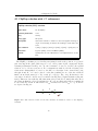
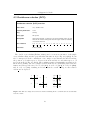
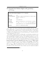
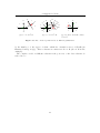
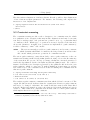
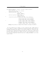
SparQ User Manual V0.6
Jan Oliver Wallgrün, Lutz Frommberger, Frank Dylla, Diedrich Wolter
SFB/TR 8 Report No. 007-07/2006
Report Series of the Transregional Collaborative Research Center SFB/TR 8 Spatial Cognition
Universität Bremen / Universität Freiburg
Contact Address:
Dr. Thomas Barkowsky
SFB/TR 8
Universität Bremen
P.O.Box 330 440
28334 Bremen, Germany
© 2006 SFB/TR 8 Spatial Cognition
Tel +49-421-218-8625
Fax +49-421-218-8620
[email protected]
www.sfbtr8.uni-bremen.de
SFB/TR 8 Spatial Cognition - Project R3-[Q-Shape]
SparQ User Manual V0.6
Jan Oliver Wallgr¨
un
Lutz Frommberger
Frank Dylla
Diedrich Wolter
July 28, 2006
Contents
1 Introduction
3
2 Installation of SparQ
2.1 Prerequisites . . . . . . . . . . . . . . . . . . . . . . . . . . . . . . . . . .
2.2 Obtaining the source code . . . . . . . . . . . . . . . . . . . . . . . . . . .
2.3 Building the binaries . . . . . . . . . . . . . . . . . . . . . . . . . . . . . .
5
5
5
5
3 Reasoning with Qualitative Spatial Relations
3.1 What is a qualitative spatial calculus? . . . . . . . . . . .
3.2 Constraint networks, consistency, and consistent scenarios
3.3 Binary and ternary spatial calculi . . . . . . . . . . . . . .
3.4 Ternary calculi and their operations . . . . . . . . . . . .
3.5 Path-consistency and backtracking search . . . . . . . . .
.
.
.
.
.
.
.
.
.
.
.
.
.
.
.
.
.
.
.
.
.
.
.
.
.
.
.
.
.
.
6
. 6
. 7
. 9
. 10
. 11
4 Supported Calculi
4.1 FlipFlop calculus with LR refinement . . . . . .
4.2 Singlecross calculus (SCC) . . . . . . . . . . . . .
4.3 Doublecross calculus (DCC) . . . . . . . . . . . .
4.4 Dipole calculus family . . . . . . . . . . . . . . .
4.5 Oriented Point Relation Algebra with granularity
4.6 The Region Connection Calculus family (RCC) .
4.7 Allen’s Interval Algebra (IA) . . . . . . . . . . .
. . . . . . . .
. . . . . . . .
. . . . . . . .
. . . . . . . .
m (OPRAm )
. . . . . . . .
. . . . . . . .
.
.
.
.
.
.
.
.
.
.
.
.
.
.
.
.
.
.
.
.
.
.
.
.
.
.
.
.
.
.
.
.
.
.
.
.
.
.
.
.
.
.
13
15
16
17
18
20
22
24
5 Using SparQ
5.1 Qualify . . . . . . . . . . . . . . . . .
5.2 Compute-relation . . . . . . . . . . . .
5.3 Constraint-reasoning . . . . . . . . . .
5.4 Including SparQ into own applications
5.5 Specifying calculi in SparQ . . . . . .
.
.
.
.
.
.
.
.
.
.
.
.
.
.
.
.
.
.
.
.
.
.
.
.
.
.
.
.
.
.
.
.
.
.
.
26
27
28
29
31
32
6 Outlook - Planned Extensions
.
.
.
.
.
.
.
.
.
.
.
.
.
.
.
.
.
.
.
.
.
.
.
.
.
.
.
.
.
.
.
.
.
.
.
.
.
.
.
.
.
.
.
.
.
.
.
.
.
.
.
.
.
.
.
.
.
.
.
.
.
.
.
.
.
.
.
.
.
.
.
.
.
.
.
34
2
1 Introduction
SparQ is a toolbox for representing space and reasoning about space based on qualitative
spatial relations. It is developed within the R3-[Q-Shape] project of the SFB/TR 8 Spatial Cognition funded by the Deutsche Forschungsgemeinschaft (DFG). SparQ is based
on results from the qualitative spatial reasoning (QSR) community which consists of
researchers from a various disciplines including computer science, artificial intelligence,
geography, philosophy, psychology, and linguistics. During the last two decades, a multitude of formal calculi over sets of spatial relations (like ‘overlaps’, ‘left-of’, ‘north-of’)
have been proposed, focusing on different aspects of space (mereotopology, orientation,
distance, etc.) and dealing with different kinds of objects (points, line segments, extended objects, etc.). SparQ aims at making these qualitative spatial calculi and the
developed reasoning techniques available in a single homogeneous framework that can
easily be included into AI applications.
The current version of SparQ provides the following services (which will be thoroughly
explained later in this manual):
qualification — A quantitative geometric description of a spatial configuration can be
transformed into a qualitative description employing one of the supported spatial
calculi.
computing with relations — The operations defined in a calculus (intersection, union,
complement, converse, composition, etc.) can be employed to perform algebraic
computations with the spatial relations from one of the supported calculi.
constraint reasoning — Techniques for solving relational constraint satisfaction problems (CSPs) based on the supported calculi can be used to check the consistency
of spatial information, determine if a particular relation can hold between certain
objects, or derive a concrete possible scenario from under-specified information.
In its current state, SparQ is a set of C libraries, calculi specifications, and a main
program written in Lisp. It is available for POSIX systems (installation is explained in
Section 2). The main program can either be used directly from the console or included
into own applications via TCP/IP streams1 . The details of using SparQ are explained
in Section 5.
1
Using the libraries directly is neither documented nor recommended as their interfaces have not been
unified so far and not all parts of the toolbox come in the form of libraries.
3
1 Introduction
Section 3 offers a small introduction to qualitative spatial calculi and qualitative spatial
reasoning in general and introduces the relevant terms required for working with SparQ.
The spatial calculi currently supported by SparQ are documented in Section 4 of this
manual. SparQ is designed in a way that makes it easy to specify and integrate new
calculi.
For an up-to-date list of supported calculi and the newest version of this manual, please
visit our website (http://www.sfbtr8.uni-bremen.de/project/r3/sparq/). For questions or feedback, please send us an e-mail to the address below. We are always interested
in suggestions for improvement and in hearing about your experience with SparQ.
The R3-[Q-Shape] team
[email protected]
4
2 Installation of SparQ
SparQ is written for POSIX systems. Its functionality is continuously tested on Linux,
Solaris and Mac OS X, but it should run on any Unix system without problems. At the
moment, there is no Windows version available. If you want to run SparQ on Windows,
please contact us.
2.1 Prerequisites
SparQ is currently not available in binary versions. To install and use SparQ, you need
ˆ gcc and g++, version 2.95 or higher
ˆ Steel Bank Common Lisp (SBCL)1 , version 0.9.10 or higher
2.2 Obtaining the source code
The source code of the actual version of SparQ and appropriate documentation is
available at the SparQ-homepage (http://www.sfbtr8.uni-bremen.de/project/r3/
sparq/).
2.3 Building the binaries
To build a running version of SparQ, unpack the source code package, enter the newly
created SparQ directory (called sparq-<version>) and run
./configure
Usually, no errors should occur and you should be able to build the SparQ executables
by running
make
All executables will be installed within the SparQ directory. If you encounter any problems during the build process, please contact the authors.
1
http://sbcl.sourceforge.net/
5
3 Reasoning with Qualitative Spatial
Relations
In this section, we provide a brief introduction on qualitative spatial reasoning and
explain the most important terms required when dealing with qualitative spatial calculi
in SparQ. For more in-depth introductions to the field, we refer to Cohn and Hazarika
(2001), Cohn (1997), Ladkin and Reinefeld (1992), Ladkin and Maddux (1994), D¨
untsch
(2005), and the references provided for particular calculi in Section 4.
3.1 What is a qualitative spatial calculus?
A qualitative calculus consists of a set of relations between objects from a certain domain
and operations defined on these relations. Let us start with an easy example: the spatial
version of the Point Algebra (PA) (Vilain et al., 1989). Imagine, we are being told about
a boat race on a river by a friend on the phone1 . We can model the river as an oriented
line and the boats of the 5 participants A,B,C,D,E as points moving along the line (see
Fig. 3.1). Thus, our domain (the set of spatial objects considered) is the set of all 1D
points.
A
B
C
E
D
A
C/D B E
Figure 3.1: A possible situation in a boat race which can be modeled by 1D points on an
oriented line and be described by qualitative relations from the Point Algebra.
We now distinguish three relations between objects from our domain. A boat can be
1
This example has been borrowed from Ligozat (2005).
6
3 Reasoning with Qualitative Spatial Relations
ahead of another boat, behind it, or on the same level. These relations can be used to
formulate knowledge about the current situation in the race. For instance, our friend
tells us the following:
1. A is behind B
2. E is ahead of B
3. A is behind C
4. D is on the same level as C
5. A is ahead of D
From this information we are able to conclude that our friend must have made an
error, probably confusing the names of the participants: We know that A is behind C
(sentence 3) and D is behind A (conversion of sentence 5). From composing these two
facts it follows that C and D cannot be on the same level which contradicts sentence 4.
On the other hand, only taking the first three sentences into account, we can conclude
that E is also ahead of A by composing the facts A is behind B (sentence 1) and B is
behind E (conversion of sentence 2). However, this information is not sufficient to derive
the exact relation between C and E, as C can either be ahead, behind or on the same
level as E.
The calculus, in this case the PA, defines a set of base relations (ahead, behind, and
same) and provides the elementary reasoning steps in the form of operations defined over
the base relations. In our small example, the applied operations were conversion, which
given the operation between x and y returns the relation between y and x (thus the
converse of ahead is behind ), and composition which takes the relations holding between
X & Y and Y & Z and returns the relation holding between X & Z (e.g. composition of
ahead and ahead is ahead ).
Often the result of operations like the composition operation is not a single base
relation but the union of more than one. For instance, knowing that X is ahead of Y and
Y is behind Z yields the union of ahead, behind, and same. Because of this, the set of
relations considered in a spatial calculus is not just the set of base relations, but the set
of all unions of base relations including the empty set and the union of all base relations
(the universal relation). All operations of the calculus are then defined for all unions of
base relations: For example, we can apply conversion to the information that X is either
ahead or at the same level as Y to infer that Y is either behind or at the same level as
X.
7
3 Reasoning with Qualitative Spatial Relations
3.2 Constraint networks, consistency, and consistent scenarios
A spatial configuration of a finite set of objects from the domain as given by sentences 1–
5 can be described as a constraint network as shown in Fig. 3.2. It consists of a variable
for each object represented by the nodes of the network and edges labeled with relations
from the considered calculus denoted as sets of base relations. For instance, sentence 1
is represented by the edge going from A to B labeled with {behind}. If no edge connects
two nodes, this corresponds to an edge labeled with the universal relation U, which is
usually omitted.
B
{behind}
A
{behind}
{ahead}
C
E
{same}
{ahead}
D
Figure 3.2: The situation described by sentences 1–5 as a constraint network.
As we have seen in our example, the information given in a constraint network can be
inconsistent. This means, no objects from the domain can be assigned to the variables
so that all the constraints given by the spatial relations annotated to the edges are
satisfied. If, on the other hand, such an assignment can be found, the constraint network
is said to be consistent or satisfiable or realizable. Determining whether a constraint
network is consistent is a fundamental problem of qualitative spatial reasoning. Special
techniques for determining consistency based on the operations of the calculus (especially
the composition operation) have been developed. However, it is important to note that
the soundness of these methods depends on the properties of the calculus at hand and
are often still subject of ongoing investigations. For more details on this issue, we refer
to Renz and Ligozat (2005) and the literature on individual calculi listed in Section 4.
A constraint network in which every constraint between two variables is a base relation
is called atomic or a scenario. This means all spatial relations between two objects
are completely determined with respect to the employed calculus and the remaining
questions is if the network is consistent or not. However, if a constraint network contains
relations that are not base relations like in Fig. 3.3(a), we might also be interested in
finding a scenario that is a refinement of the original network (meaning it has been
derived by removing individual base relations from the sets annotated to the edges)
and that is consistent. Fig. 3.3(b) shows such a consistent scenario for the network in
8
3 Reasoning with Qualitative Spatial Relations
Fig. 3.3(a). If such a consistent scenario can be found, we also know that the original
network is consistent. Otherwise, we know it is inconsistent. Of course, it is possible
that more than one consistent scenario exists for a given constraint network and we
might be interested in finding only one or all of these. An alternative consistent scenario
is depicted in Fig. 3.3(c).
C
{behind}
A
C
{behind}
{ahead,behind}
B
{behind}
A
(a)
C
{behind}
{ahead}
B
(b)
{behind}
A
{behind}
{behind}
B
(c)
Figure 3.3: A non-atomic constraint network (a) with possible consistent scenarios (b) and (c).
The problems of determining consistency and finding consistent scenarios are subsumed under the term constraint-based reasoning throughout this text.
3.3 Binary and ternary spatial calculi
After giving a rather intuitive introduction to qualitative spatial calculi, we want to give
a more formal definition of a spatial calculus and especially the operations that need to
be defined for a calculus. This set of operations differs depending on whether we are
dealing with a binary calculus (like the PA) in which all relations relate two objects or
with a ternary calculus in which all relations relate three objects.
As we have seen an n-ary qualitative spatial calculus consists of:
1. a domain D which contains the considered spatial objects (D could for instance
be the R2 when we are considering point objects in the plane)
2. a finite set BR of n-ary relations on D which are called base relations (typically
the set of base relations is jointly exhaustive and pairwise disjoint which means
that exactly one of the base relations holds for each n-tuple from D)
3. a finite overall set of relations R that is derived from BR by taking all possible
unions of base relations (as we have seen, it is common to write these relations as
sets of base relations, in which case R = 2BR )
4. a set of operations closed over R
9
3 Reasoning with Qualitative Spatial Relations
Let us now turn to the operations that need to be defined. As all relations for a given
calculus are subsets of tuples from the same Cartesian product, the three set operations
union, intersection, and complement are already defined for every calculus independent
of its arity:
Union: R ∪ S = { x | x ∈ R ∨ x ∈ S }
Intersection: R ∩ S = { x | x ∈ R ∧ x ∈ S }
Complement: R = U \ R = { x | x ∈ U ∧ x 6∈ R }
where R and S are relations from R.
Using our set notation for relations from R, these set operations directly transfer
to these sets. For example, the intersection of the PA relations {behind, same} and
{same, ahead} is the relation {same} and the complement of {same} is {behind, ahead}.
The other operations depend on the arity of the calculus.
Operations of binary calculi
For binary calculi, two more operations are utilized. These are the converse and composition operations, we have already encountered above:
Converse: R` = { (y, x) | (x, y) ∈ R }
Composition: R ◦ S = { (x, z) | ∃y ∈ D : ((x, y) ∈ R ∧ (y, z) ∈ S) }
Again, here are two examples from the PA: The converse of {behind} is {ahead} and
the composition of {ahead} and {ahead, same} is {ahead} (if A is ahead of B and B is
ahead or at the same level as C than A has to be ahead of C).
For some calculi, the composition operation defined does not comply to the “strong”
definition above, as this would result in a composition that is not closed for the set of
relations R (and no finite set of relations including the base relations exists for which
this is the case). In this case, the used composition operation is the “weak” composition
that takes the union of all base relations that have a non-empty intersection with the
result of the strong composition:
Weak composition: R ◦weak S = { d | T ∈ BR ∧ d ∈ T ∧ T ∩ (R ◦ S) 6= ∅ }
For some calculi, it is not yet known whether the defined composition operation is
“strong” or not.
10
3 Reasoning with Qualitative Spatial Relations
3.4 Ternary calculi and their operations
While there is only one possibility to permute the two objects of a binary relation which
leads to the converse operation, there exist 5 such permutations for the three objects of
a ternary relation. This results in the following 5 operations introduced in Zimmermann
and Freksa (1996):
Inverse: INV(R) = { (y, x, z) | (x, y, z) ∈ R }
Short cut: SC(R) = { (x, z, y) | (x, y, z) ∈ R }
Inverse short cut: SCI(R) = { (z, x, y) | (x, y, z) ∈ R }
Homing: HM(R) = { (y, z, x) | (x, y, z) ∈ R }
Inverse homing: HMI(R) = { (z, y, x) | (x, y, z) ∈ R }
It is in general not needed to specify all these operations as some can be expressed by
others, but they are all available in SparQ nonetheless. Composition for ternary calculi
is defined accordingly to the binary case:
Composition: R ◦ S = { (w, x, z) | ∃y ∈ D : ((w, x, y) ∈ R ∧ (x, y, z) ∈ S) }
Other ways of composing two ternary relations can be expressed as a combination of
the unary permutation operations and the composition (Scivos and Nebel, 2001) and
thus do not have to be defined separately and are also not accessible individually in
SparQ. The definition of weak composition is identical to the binary case.
As we have not introduced a ternary calculus so far, we resign from giving any examples
here, but some can be found later in Section 5.
3.5 Path-consistency and backtracking search
Determining consistency of a constraint network in which the constraints are given as
qualitative spatial relations from a particular calculus, is a particular instance of a constraint satisfaction problem (CSP). Unfortunately, the domains of our variables are typically infinite (e.g. the set of all points in the plane) and thus backtracking over all the
values of the domain cannot be used to determine consistency.
The techniques developed for relational constraint problems are instead based on
weaker forms of consistency called local consistencies which can be tested or enforced
based on the operations of the calculus and which are under particular conditions sufficient to decide consistency.
11
3 Reasoning with Qualitative Spatial Relations
One important form of local consistency is path-consistency which (in binary CSPs)
means that for every triple of variables each consistent evaluation of the first two variables can be extended to the third variable in such a way that all constraints are satisfied.
In the best case, path-consistency decides consistency for a given calculus. This means,
that if we can make the network path-consistent by possibly removing some base relations from the constraints without ending up with the empty relation, we know that
the original network is consistent. If this cannot be achieved, the network has to be
inconsistent. Unfortunately, it is usually not the case that path-consistency decides
consistency.
However, sometimes path-consistency is sufficient to decide consistency at least for
a subset S of the relations from R, for instance the set of base relations. On the one
hand, this means that whenever our constraint networks only contains labels which are
base relations, we again can use path-consistency as a criterion to decide consistency.
On the other hand, if the subset S exhaustively splits R (which means that every relation from R can be expressed as a union of relations from S), this at least allows to
formulate a backtracking algorithm to determine consistency by recursively splitting the
constraints and using path-consistency as a decision procedure for the resulting CSPs
with constraints from S (Ladkin and Reinefeld, 1992).
To enforce path-consistency, syntactic procedures called algebraic closure algorithms
have been developed that are based on the operations of the calculus (the composition
operation in particular) and work in O(n3 ) time for binary calculi and O(n4 ) for ternary
calculi where n is the number of variables. But again, we have to note that these syntactic
procedures do not necessarily yield the correct results with respect to path-consistency
as defined above. Whether algebraic closure coincides with path-consistency needs be
investigated for each calculus individually and we again refer to the literature listed in
the individual calculus descriptions in Section 4.
12
4 Supported Calculi
In this section, we briefly describe the spatial calculi currently supported by SparQ.
Some calculi are actually calculi families for which a set of calculus parameters needs
to be specified in order to obtain a particular calculus instance. For instance, for the
OPRAm calculus the granularity (number of partitioning lines) has to be specified as a
calculus parameter.
Each calculi description in this section starts with a box summarizing the main characteristics of the considered calculus. The meaning of the entries in the box are explained
below:
short name — the name used in SparQ to refer to this calculus
calculus parameters — the parameters that need to be specified whenever using this
calculus
arity — the arity of the relations of this calculus (binary or ternary)
entity type — the spatial entities related in this calculus (2D points, oriented 2D points,
line segments dipoles), etc.)
description — a short description of the calculus
base relations — a naming scheme or list of the base relations of the calculus
references — references to literature about this calculus
remarks — special remarks concerning the calculus
A quick overview on the implemented calculi is given in Tab. 4.1 which also classifies
the calculi according to their arity (binary, ternary), their domain (points, oriented
points, line segments, regions), and the aspect of space modeled (orientation, distance,
mereotopology).
13
4 Supported Calculi
Calculus
FFC/LR
SCC
DCC
DRAc
OPRAm
RCC-5/8*
Interval algebra*
arity
domain
aspect of space
binary ternary
point or. point line seg. region
orient. dist. mereot.
3
3
3
3
3
3
3
3
3
3
3
3
3
3
3
3
3
3
3
Table 4.1: The calculi currently included in SparQ. For entries marked by a ‘∗’ no qualifier is
available yet. Allen’s Interval Algebra is originally intended for temporal reasoning, but can also
be interpreted spatially.
14
4 Supported Calculi
4.1 FlipFlop calculus with LR refinement
FlipFlop calculus (FFC) overview
short name
ffc, ff, flipflop
calculus parameters
none
arity
ternary
entity type
2D points
description
base relations
relates the referent C relative to the line segment starting at
origin A and ending at relatum B resulting in seven base relations
l (left), r (right), f (front), b (back), s (start), e (end), dou, tri
references
Ligozat (1993), Scivos and Nebel (2005)
remark
SparQ uses the LR refinement in its implementation of the
FFC
The FlipFlop calculus proposed in Ligozat (1993) describes the position of a point C
(the referent) in the plane with respect to two other points A (the origin) and B (the
relatum) as illustrated in Fig. 4.1. It can for instance be used to describe the spatial
relation of C to B as seen from A. For configurations with A 6= B the following base
relations are distinguished: C can be to the left or to the right of the oriented line going
through A and B, or C can be placed on the line resulting in one of the five relations
inside, f ront, back, start (C = A) or end (C = B) (cp. Fig. 4.1). Relations for the
case where A and B coincide were not included in Ligozat’s original definition (Ligozat,
1993). This was done with the LR refinement (Scivos and Nebel, 2005) that introduces
the relations dou (A = B 6= C) and tri (A = B = C) as additional relations, resulting in
9 base relations overall. A LR relation relLR is written as A, B relLR C, e.g. A, B r C
as depicted in Fig. 4.1.
s
A
l
r
e
B
C
Figure 4.1: The reference frame for the LR calculus, an enhanced version of the FlipFlop
Calculus
15
4 Supported Calculi
4.2 Singlecross calculus (SCC)
Singlecross calculus (SCC) overview
short name
scc
calculus parameters
none
arity
ternary
entity type
2D points
description
base relations
relates the referent c relative to the line between origin a and
relatum b and the orthogonal line thru b, resulting in nine relations
0..7 and b (for b=c)
references
Freksa (1992a)
The single cross calculus is a ternary calculus that describes the direction of a point C
(the referent) with respect to a point B (the relatum) as seen from a third point A (the
origin). It has originally been proposed in Freksa (1992a). The plane is partitioned into
regions by the line going through A and B and the perpendicular at B. This results in
eight possible directions for C as illustrated in Fig. 4.2. We denote these base relations
by numbers from 0 to 7 instead of using linguistic prepositions, e.g. 2 instead of left, as
originally done in Freksa (1992a). Relations 0, 2, 4, 6 are linear ones, while relations 1,
3, 5, 7 are planar. In addition, three special relations exist for the cases A 6= B = C
(bc), A = B 6= C (dou), and A = B = C (tri). A single cross relation relSCC is written
as A, B relSCC C, e.g. A, B 4 C or A, B dou C. The relation depicted in Fig. 4.2 is the
relation A, B 5 C.
1
2
0
B
7
6
C
3
A
5
4
Figure 4.2: The Single Cross Reference System
16
4 Supported Calculi
4.3 Doublecross calculus (DCC)
Doublecross calculus (DCC) overview
short name
dcc, double-cross
calculus parameters
none
arity
ternary
entity type
2D points
description
relates the referent C relative to the line between origin A and
relatum B and the orthogonal lines through A and B, resulting
in 17 base relations
0 4, 1 5, 2 5, 3 5, 3 6, 3 7, 4 0, 5 1, 5 2, 5 3, 6 3, 7 3,
4 4, 4 b, 4 a
base relations
references
Freksa (1992a)
The double cross calculus (Freksa, 1992a) can be seen as an extension of the single
cross calculus adding another perpendicular, this time at A (see Fig. 4.3 (right)). It can
also be interpreted as the combination of two single cross relations, the first describing
the position of C with respect to B as seen from A and the second with respect to A
as seen from B (cf. Fig. 4.3 (left)). The resulting partition distinguishes 13 relations (7
linear and 6 planar) denoted by tuples derived from the two underlying SCC reference
frames and four special cases, A = C 6= B (4 a), A 6= B = C (b 4), A = B 6= C (dou),
and A = B = C (tri), resulting in 17 base relations overall. In Fig. 4.3 the relation
A, B 5 3 C is depicted.
1
0
7
2
B
6
3
A
5
6
4
1_5 0_4 7_3
4
5
7
B
3
2_5
A
2
3_6
1
3_7 4_0 5_1
0
B 6_3
C
3_5 4_4 5_3
A 5_2
Figure 4.3: The two Single Cross reference frames resulting in the overall Double Cross Calculus
reference frame
17
4 Supported Calculi
4.4 Dipole calculus family
A dipole is an oriented line segment as e.g. determined by a start and an end point. We
will write d~AB for a dipole defined by start point A and end point B. The idea of using
dipoles was first introduced by Schlieder (1995) and extended resulting in the coarsegrained Dipole Relation Algebra DRAc (Moratz et al., 2000). Later, a fine-grained
version of the dipole calculus (DRAf ) has been proposed (Dylla and Moratz, 2005)
and which has further been extended to DRAf p (Dylla and Moratz, 2005). In SparQ,
currently only the coarse-grained version DRAc is available.
Coarse-grained Dipole Relation Algebra (DRAc )
Coarse-grained dipole calculus (DRAc ) overview
short name
dra-24, dipole-coarse
calculus parameters
none
arity
binary
entity type
dipoles in the plane (oriented line segments)
description
relates two dipoles using the FlipFlop relations between the
start and end point of one dipole and the other dipole
base relations
4-symbol words where each symbol can be either l (left), r
(right), s (start), or e (end) (not all combinations are possible)
references
Moratz et al. (2000)
A
B
D
C
Figure 4.4: A dipole configuration: d~AB rlll d~CD in the coarse-grained dipole relation algebra
(DRAc ).
The coarse-grained dipole calculus variant (DRAc ) describes the orientation relation
between two dipoles d~AB and d~CD with the preliminary of A, B, C, and D being in
general position, i.e. no three disjoint points are collinear. Each base relation is a 4-
18
4 Supported Calculi
tuple (r1 , r2 , r3 , r4 ) of FlipFlop relations relating a point from one of the dipoles with
the other dipole. r1 describes the relation of C with respect to the dipole d~AB , r2 of
D with respect to d~AB , r3 of A with respect to d~CD , and r4 of B with respect to d~CD .
The distinguished FlipFlop relations are left, right, start, and end (see Fig. 4.1). Dipole
relations are usually written without commas and parentheses, e.g. rrll. Thus, the
example in Fig. 4.4 shows the relation d~AB rlll d~CD . Since the underlying points for
a DRAc relation need to be in general position, ri can only take the values left, right,
start, or end resulting in 24 base relations.
19
4 Supported Calculi
4.5 Oriented Point Relation Algebra with granularity m
(OPRAm )
Oriented Point Relation Algebra (OPRAm ) overview
short name
opra
calculus parameters
granularity - number of partitioning lines (= number of planar
relations / 2), must be > 0
arity
binary
entity type
oriented 2D points
description
relates two oriented points a and b with respect to granularity
m
[i, j] with i, j ∈ {0, .., 4m − 1}, if a and b have different positions; [i] with i ∈ {0, .., 4m − 1} if they have the same position
base relations
references
Moratz et al. (2005), Moratz (2006)
The domain of the Oriented Point Relation Algebra (OPRAm ) (Moratz et al., 2005,
Moratz, 2006) is the set of oriented points (points in the plane with an additional direction parameter). The calculus relates two oriented points with respect to their relative
~ can be described by its Cartesian
orientation towards each other. An oriented point O
coordinates xO , yO ∈ R and a direction φO~ ∈ [0, 2π] with respect to an absolute reference
direction and thus D = R2 × [0, 2π].
The OPRAm calculus is suited for dealing with objects that have an intrinsic front
or move in a particular direction and can be abstracted as points. The exact set of base
relations distinguished in OPRAm depends on the granularity parameter m ∈ N. For
each of the two related oriented points, m lines are used to partition the plane into 2m
planar and 2m linear regions. Fig. 4.5 shows the partitions for the cases m = 2 (a) and
~ and
m = 4 (b). The orientation of the two points is depicted by the arrows starting at A
~
B, respectively. The regions are numbered from 0 to 4m − 1; region 0 always coincides
with the orientation of the point. An OPRAm base relation relOPRAm consists of a pair
~ which contains B,
~ while j is the number
(i, j) where i is the number of the region of A
~
~
~ m∠j B
~
of the region of B that contains A. These relations are usually written as A
i
~ and
~ 2∠ 1 B
with i, j ∈ Z4m 1 . Thus, the examples in Fig. 4.5 depict the relations A
7
3
~
~
A 4∠13 B. Additional base relations called same relations describe situations in which
the positions of both oriented points coincide. In these cases, the relation is determined
1
Z4m defines a cyclic group with 4m elements.
20
4 Supported Calculi
0
0
6
1
1
7
2
7
A
3
5
B
4
4
~
~ 2∠17 B
(a) m = 2: A
5
2
3
4
5
0 15 14
1 0
3
13
6
B
A
7
8
9 10
0
13
12
11
7 8
~
~ 4∠313 B
(b) m = 4: A
9
10
1
2
B
3
A
7
6
4
5
~ and B
~ coincide:
(c) case where A
~ 2∠1 B
~
A
Figure 4.5: Two oriented points related at different granularities.
~ into which the orientation arrow of B
~ falls (as
by the number s of the region of A
~ 2∠s B
~ (A
~ 2∠1 B
~ in the
illustrated in Fig. 4.5(c)). These relations are written as A
example).
The complete set R of OPRAm relations is the power set of the base relations described above.
21
4 Supported Calculi
4.6 The Region Connection Calculus family (RCC)
The calculi from the RCC family (RCC-8 and RCC-5) allow mereotopological reasoning
(reasoning about connection and part-of relationships) about simple regions in the plane.
Other domains involving regions can also be considered in the context of RCC, e.g. 3D
regions, or non-simple regions in the plane, which can affect the correctness of the
constraint-based reasoning algorithms. Since so far no qualifier for RCC is available in
SparQ, the exact domain is actually still not determined. However, we will assume the
case of simple regions in the plane in the following.
RCC-8
Region Connection Calculus 8 (RCC-8) overview
short name
rcc-8
calculus parameters
none
arity
binary
entity type
simple regions in the plane
description
describes the mereotopological relation between two regions
base relations
dc (disconnected), ec (externally connected), po (partially overlapping), eq (equal), tpp (tangential proper part), ntpp (nontangential proper part), tppi (tangential proper part inverse),
nttpi (non-tangential proper part inverse)
references
Randell et al. (1992), Cohn et al. (1997)
remarks
no qualifier is available for this calculus yet
RCC-8 is the more fine-grained variant of RCC calculi. It distinguishes the eight base
relations dc (disconnected), ec (externally connected), po (partially overlapping), eq
(equal), tpp (tangential proper part), ntpp (non-tangential proper part), tppi (tangential
proper part inverse), and nttpi (non-tangential proper part inverse) which are illustrated
in Fig. 4.6.
22
4 Supported Calculi
a dc b
a ec b
a po b
a eq b
disconnected
externally
connected
partially
overlapping
equal
a tpp b
a ntpp b
a tppi b
a nttpi b
tangential non-tangential tangential proper non-tangential
proper part inverse
proper part proper part
part inverse
Figure 4.6: The RCC-8 base relations.
RCC-5
Region Connection Calculus 5 (RCC-5) overview
short name
rcc-5
calculus parameters
none
arity
binary
entity type
simple regions in the plane
description
describes the mereotopological relation between two regions
base relations
dr (discrete from), po (partially overlapping), eq (equal), pp
(proper part), ppi (proper part inverse)
references
Cohn et al. (1997)
remarks
no qualifier is available for this calculus yet
RCC-5 is a coarser version of RCC-8. The RCC-8 relations dc and ec are combined
into one relation called dr. Similarly, nttp and ttp are combined into pp and nttpi and
ttpi into ppi.
23
4 Supported Calculi
4.7 Allen’s Interval Algebra (IA)
Allen’s Interval Algebra overview
short name
allen, aia, ia
calculus parameters
none
arity
binary
entity type
intervals (defined by a start and end-point) on a unidirectional
time line
describes the mereotopological relation between two intervals
description
base relations
b (before), bi (before inverse), m (meets), mi (meets inverse),
o (overlaps), oi (overlaps inverse), s (starts), si (starts inverse),
d (during), di (during inverse), f (finishes), fi (finishes inverse),
eq (equals)
references
Allen (1983)
remarks
no qualifier is available for this calculus yet
Allen’s interval algebra (IA) (Allen, 1983) relates pairs of time intervals. A time
interval x can be represented as a tuple of a starting point xs and end point xe (hxs , xe i)
of real numbers with xs < xe . 13 base relations are distinguished (cf. Tab. 4.2): before,
meets, overlaps, starts, during, f inishes, before inverse, meets inverse, overlaps inverse,
starts inverse, during inverse, f inishes inverse, equals. The relations can be defined
by comparing the start and end points of the intervals (see Tab. 4.2). The converse
operation always takes an interval relation r to the corresponding inverse relation, e.g. f
to fi.
24
4 Supported Calculi
Basic relation (abbrv.)
Example
Condition
x before y
y after x
(b)
(bi)
xxx
xe < ys
x meets y
y met-by x
(m)
(mi)
xxxx
yyy
xe = ys
yyyy
x overlaps y
(o)
y overlapped-by x (oi)
xxxxx
yyyyy
xs < ys < xe ∧
xe < ye
x during y
y includes x
(d)
(di)
xxx
yyyyyyy
xs > ys ∧
xe < ye
x starts y
y started-by x
(s)
(si)
x finishes y
y finished-by x
(f)
(fi)
x equals y
(eq)
xxx
yyyyyyy
xxx
yyyyyyy
xxxxxxx
yyyyyyy
xs = ys ∧
xe < ye
xe = ye ∧
xs > ys
xs = ys ∧
xe = ye
Table 4.2: The 13 basic Allen relations.
25
5 Using SparQ
SparQ consists of a set of modules that logically structure the different services provided,
which will be explained below. The general architecture is visualized in Fig. 5.1. The
dashed parts are extensions planned for the future (see Section 6).
qualify
neighborhood−
reasoning
specifications
SparQ
constraint−
reasoning
calculi
compute−
relation
quantify
...
interface
CASL
...
Figure 5.1: Module architecture of the SparQ toolbox.
The general syntax for using the SparQ main script which can be found in the main
directory of SparQ is as follows:
$ ./sparq <module> <calculus identifier> <module specific parameters>
Example:
$ ./sparq compute-relation dra-24 complement "(lrll llrr)"
where ‘compute-relation’ is the name of the module to be utilized, in this case the
module for conducting operations on relations, ‘dra-24’ is the SparQ identifier for the
dipole calculus DRAc , and the rest are module specific parameters, here the name of the
operation that should be conducted (‘complement’) and a string parameter representing
the disjunction of the two dipole base relations lrll and llrr 1 . The example call thus
computes the complement of the disjunction of these two relations.
1
Unions of base relations are always represented as a space-separated list of the base relations enclosed
in parentheses in SparQ.
26
5 Using SparQ
Some calculi have calculi specific parameters, for example the granularity parameter
in OPRAm . These parameters are appended with a ‘-’ after the calculus’ base identifier.
opra-3 for example refers to OPRA3 .
SparQ provides the following modules:
qualify — transforms a quantitative geometric description of a spatial configuration into
a qualitative description based on one of the supported spatial calculi
compute-relation — applies the operations defined in the calculi specifications (intersection, union, complement, converse, composition, etc.) to a set of spatial relations
constraint-reasoning — performs computations on constraint networks
We will take a closer look at each of these three modules in the next sections.
5.1 Qualify
The purpose of the qualify module is to turn a quantitative geometric scene description
into a qualitative scene description composed of base relations from a particular calculus. The calculus is specified via the calculus identifier that is passed with the call to
SparQ. Qualification is required for applications in which we want to perform qualitative
computations over objects whose geometric parameters are known.
y
5
C
B
A
0
x
5
Figure 5.2: An example configuration of three dipoles.
The qualify module reads a quantitative scene description and generates a qualitative
description. A quantitative scene description is a space-separated list of base object
descriptions enclosed in parentheses. Each base object description is a tuple consisting
of an object identifier and object parameters that depend on the type of the object. For
instance, let us say we are working with dipoles which are oriented line segments. The
object description of a dipole is of the form ‘(name xs ys xe ye )’, where name is the
identifier of this particular dipole object and the rest are the coordinates of start and
end point of the dipole. Let us consider the example in Fig. 5.2 which shows three
dipoles A, B, and C. The quantitative scene description for this situation would be:
27
5 Using SparQ
( (A -2 0 8 0) (B 7 -2 2 5) (C 1 -1 4.5 4.5) )
The qualify module has one module specific parameter that needs to be specified:
mode — This parameter controls which relations are included into the qualitative scene
description: If the parameter is ‘all’, the relation between every object and every
other object will be included. If it is ‘first2all’ only the relations between the first
and all other objects are computed in the binary case or between the first two
objects and all other objects in the ternary case.
The resulting qualitative scene description is a space-separated list of relation tuples
enclosed in parentheses. A relation tuple consists of an object identifier followed by a
relation name and another object identifier, meaning that the first object stands in this
particular relation with the second object. The command to produce the qualitative
scene description followed by the result is2 :
$ ./sparq qualify dra-24 all
$ ( (A -2 0 8 0) (B 7 -2 2 5) (C 1 -1 4.5 4.5) )
> ( (A rllr B) (A rllr C) (B lrrl C) )
If we had chosen ‘first2all’ as mode parameter the relation between B and C would not
have been included in the qualitative scene description.
5.2 Compute-relation
The compute-relation module allows to compute with the operations defined in the
calculus specification. The module specific parameters are the operation that should be
conducted and one or more input relations depending on the arity of the operation. Let
us say we want to compute the converse of the llrl dipole relation. The corresponding
call to SparQ and the result are:
$ ./sparq compute-relation dra-24 converse llrl
> (rlll)
The result is always a list of relations as operations often yield a disjunction of base
relations. In this case, however, the disjunction only contains a single relation. The
composition of two relations requires one more relation as parameter because it is a
binary operation, e.g.:
$ ./sparq compute-relation dra-24 composition llrr rllr
> (lrrr llrr rlrr slsr lllr rllr rlll ells llll lrll)
2
In all the examples, input lines start with ‘$’. Output of SparQ is marked with ‘>’.
28
5 Using SparQ
Here the result is a disjunction of 10 base relations. It is also possible to have disjunctions
of base relations as input parameters. For instance, the following call computes the
intersection of two disjunctions:
$ ./sparq compute-relation dra-24 intersection "(rrrr rrll rllr)"
"(llll rrll)"
> (rrll)
5.3 Constraint-reasoning
The constraint-reasoning module reads a description of a constraint network—which
is a qualitative scene description that may include disjunctions and may be inconsistent and/or underspecified—and performs an operation on it, e.g., a particular kind
of consistency check. Which type of operation is executed depends on the first module specific parameter. Actually, four operations are implemented: ‘path-consistency’,
‘scenario-consistency’, ‘refine’3 and ‘extend’.
action — The actions currently provided are ‘path-consistency’ and ‘scenario-consistency’ which determine which kind of consistency check is performed, as well as ‘refine’
and ‘extend’ which perform set operations on constraint networks.
The action ‘path-consistency’ causes the module to enforce path-consistency on the constraint network using van Beek’s algorithm (van Beek, 1992) or detect the inconsistency
of the network in the process. In case of ternary calculus the canonical extension of
van Beek’s algorithm as described in Dylla and Moratz (2004) is used. We could for
instance check if the scene description generated by the qualify module in Section 5.1 is
path-consistent—which of course it is. To make it slightly more interesting, we add the
base relation ells to the constraint between A and C resulting in a constraint network
that is not path-consistent:
$
$
>
>
./sparq constraint-reasoning dra-24 path-consistency
( (A rllr B) (A (ells rllr) C) (B lrrl C) )
Modified network.
( (B (lrrl) C) (A (rllr) C) (A (rllr) B) )
The result is a path-consistent constraint network in which ells has been removed. The
output ‘Modified network’ indicates that the original network was not path-consistent
and had to be changed. Otherwise, the result would have started with ‘Unmodified
network’. In the next example we remove the relation rllr from the disjunction between
A and C. This results in a constraint network that cannot be made path-consistent
which implies that it is not globally consistent.
3
In former versions of SparQ, the ‘refine’ action was called ‘merge’. This naming is still valid for
backward compatibility reasons but may vanish in the future.
29
5 Using SparQ
$
$
>
>
./sparq constraint-reasoning dra-24 path-consistency
( (A rllr B) (A ells C) (B lrrl C) )
Not consistent.
( (B (lrrl) C) (A () C) (A (rllr) B) )
SparQ correctly determines that the network is inconsistent and returns the constraint
network in the state in which the inconsistency showed up (indicated by the empty
relation () between A and C).
In a last path-consistency example we use the ternary double cross calculus:
$
$
>
>
./sparq constraint-reasoning dcc path-consistency
( (A B (7_3 6_3) C) (B C (7_3 6_3 5_3) D) (A B (3_6 3_7) D) )
Not consistent.
( (A B (3_6 3_7) D) (A B (6_3 7_3) C) (B C (5_3 6_3 7_3) D) (D C () A) )
If ‘scenario-consistency’ is provided as argument, the constraint-reasoning module
checks if a path-consistent scenario exists for the given network. It uses a backtracking
algorithm to generate all possible scenarios and checks them for path-consistency as
described above. A second module specific parameter determines what is returned as
the result of the search:
return — This parameter determines what is returned in case of a constraint network for
which path-consistent scenarios can be found. It can take the values ‘first’ which
returns the first path-consistent scenario, ‘all’ which returns all path-consistent
scenarios, and ‘interactive’ which returns one solution and allows to ask for the
next solution until all solutions have been iterated.
Path-consistency is also used as a forward-checking method during the search to make
it more efficient. For certain calculi, the existence of a path-consistent scenario implies
global consistency. However, this again has to be investigated for each calculus. As a
future extension it is planned to allow to specify splitting subsets of a calculus for which
path-consistency implies global consistency and provide a variant of the backtracking
algorithm that decides global consistency by searching for path-consistent instantiations
that only contain relations from the splitting subset.
In the following example, we use ‘first’ as additional parameter so that only the first
solution found is returned:
$ ./sparq constraint-reasoning dra-24 scenario-consistency first
$ ( (A rele C) (A ells B) (C errs B) (D srsl C) (A rser D) (D rrrl B) )
> ( (B (rlrr) D) (C (slsr) D) (C (errs) B) (A (rser) D) (A (ells) B)
(A (rele) C) )
30
5 Using SparQ
In case of an inconsistent constraint network, SparQ returns ‘Not consistent.’ as in the
following example:
$ ./sparq constraint-reasoning dra-24 scenario-consistency first
$ ( (A rele C) (A ells B) (C errs B) (D srsl C) (A rser D) (D rllr B) )
> Not consistent.
The action ’refine’ returns the disjunction of two constraint networks. Analogously,
’extend’ returns the conjunction:
$ ./sparq constraint-reasoning dra-24 refine
$ ( (A (rele errs) B) ) ( (A errs B) )
> ( (A errs B) )
$ ./sparq constraint-reasoning dra-24 extend
$ ( (A rele B) ) ( (A errs B) )
> ( (A (rele errs) B) )
5.4 Including SparQ into own applications
SparQ can also run in server mode which makes it easy to integrate it into own applications. We have chosen a client/server approach as it allows for straightforward
integration independent of the programming language used for implementing the application.
When run in server mode, SparQ takes TCP/IP connections and interacts with the
client via simple plain-text line-based communication. This means the client sends commands which consist of everything following the ‘./sparq’ in the examples in this text,
and can then read the results from the TCP/IP stream.
SparQ is started in server mode by providing the command line option --interactive
(-i), optionally followed by --port (-p) to specify the port.
$ ./sparq --interactive --port 4443
If no port is given, SparQ interacts with standard-input and standard-output, i.e., it can
be used interactively from the shell.
An example of client/server communication with SparQ is given in Listing 5.1 which
shows a small Python script that opens a connection to the server and performs some simple computations (qualification, adding another relation, checking for path-consistency).
It produces the following output:
>
>
>
>
( (A rrll B) (A rrll C) )
( (A rrll B) (A rrll C) (B eses C) )
Not consistent.
( (B (eses) C) (A () C) (A (rrll) B) )
31
5 Using SparQ
5
10
15
# connect to sparq server on localhost , port 4443
sock = socket . socket ( socket . AF_INET , socket . SOCK_STREAM )
sock . connect (( ’ localhost ’ , 4443))
sockfile = sock . makefile ( ’r ’)
# qualify a geometrical scenario with DRA -24
sock . send ( ’ qualify dra -24 first2all ’)
sock . send ( ’ (( A 4 6 9 0.5) ( B -5 5 0 2) ( C -4 5 6 0)) ’)
scene = readline ()
# read the answer
print scene
# add an additional relation ( B eses C )
sock . send ( ’ constraint - reasoning dra -24 refine ’)
sock . send ( scene + ’( B eses C ) ’)
scene2 = readline ()
# read the answer
print scene2
# check the new scenario for consistency
sock . send ( ’ constraint - reasoning dra -24 path - consistency ’)
sock . send ( scene2 )
print readline ()
# print the answer
print readline ()
# print the resulting constraint network
Listing 5.1: Integrating SparQ into own applications: an example in Python
5.5 Specifying calculi in SparQ
For most calculi it should be rather easy to include them into SparQ. The main thing
that has to be done is to provide the calculus specification. Listing 5.2 shows an extract
of the definition of a simple exemplary calculus for reasoning about distances between
three point objects distinguishing the three relations ‘closer’, ‘farther’, and ‘same’. The
specification is done in Lisp-like syntax.
The arity of the calculus, the base relations, the identity relation and the different
operations have to be specified, using lists enclosed in parentheses (e.g. when an operation
returns a disjunction of base relations). In this example, the inverse operation applied to
‘same’ yields ‘same’ and composing ‘closer’ and ‘same’ results in the universal relation
written as the disjunction of all base relations. It is not required to specify the homing,
inverse short cut, and inverse homing operations (cmp. Section 3.4) as these can be
computed by applying the other operations (e.g. inverse of short cut yields inverse short
cut). It is principally possible to leave more operations unspecified. However, this may
mean that certain computations cannot be performed for this calculus.
In addition to the calculus specification, it is necessary to provide the implementation
of a qualifier function which for an n-ary calculus takes n geometric objects of the
corresponding base type as input and returns the relation holding between these objects.
The qualifier function encapsulates the methods for computing the qualitative relations
from quantitative geometric descriptions. If it is not provided, the qualify module will
not work for this calculus.
32
5 Using SparQ
5
10
15
( def-calculus " Relative distance calculus ( reldistcalculus ) "
: arity : ternary
: base-relations ( same closer farther )
: identity-relation same
: inverse-operation (( same same )
( closer closer )
( farther farther ))
: shortcut-operation (( same same )
( closer farther )
( farther closer ))
: c omp osit ion-o pera tion (( same same ( same closer farther ))
( same closer ( same closer farther ))
( same farther ( same closer farther ))
( closer same ( same closer farther ))
( closer closer ( same closer farther ))
( closer farther ( same closer farther ))
( farther same ( same closer farther ))
( farther closer ( same closer farther ))
( farther farther ( same closer farther ))))
Listing 5.2: Specification of a simple ternary calculus for reasoning about distances.
For some calculi, it is not possible to provide operations in form of simple tables as
in the example. For instance, OPRAm has an additional parameter that specifies the
granularity and influences the number of base relations. Thus, the operations can only
be provided in procedural form, meaning the result of the operations are computed from
the input relations when they are required. For these cases, SparQ allows to provide
the operations as implemented functions and uses a caching mechanism to store often
required results.
33
6 Outlook - Planned Extensions
Besides extending the set of supported qualitative calculi, the following extensions are
currently planned for the future:
neighborhood-based reasoning — a module for reasoning based on the notion of conceptual neighborhood (Freksa, 1992b) that could for instance be used for constraint
relaxation and spatial planning
quantification — a module that analogous to the qualify module takes a consistent
qualitative scene description and turns it into a prototypical quantitative scene
description
geometric reasoning based on Gr¨
obner bases — a module intended for calculus developers that for instance allows to derive composition tables automatically from
algebraic descriptions of the base relations of the calculus (cmp. Moratz et al.,
2000)
interfaces & XML specification — interfaces to exchange calculus specifications with
other QSR frameworks (e.g. W¨olfl and Mossakowski, 2005) and a general XML
format for the specification of qualitative calculi
Further goals are to continue the optimization of the algorithms employed in SparQ, for
instance by applying maximal tractable subsets for the constraint reasoning part, and to
include new results from the QSR community as they become available, in particular with
respect to constraint reasoning techniques for calculi for which the standard algebraic
closure algorithms are insufficient to decide consistency.
Again, please feel free to contact us if you have any ideas or wishes concerning the
extension or improvement of SparQ.
34
Bibliography
J. F. Allen. Maintaining knowledge about temporal intervals. Communications of the
ACM, pages 832–843, November 1983.
A G Cohn, B Bennett, J M Gooday, and N Gotts. RCC: A calculus for region based
qualitative spatial reasoning. GeoInformatica, 1:275–316, 1997.
Anthony G. Cohn. Qualitative spatial representation and reasoning techniques. In
Gerhard Brewka, Christopher Habel, and Bernhard Nebel, editors, KI-97: Advances
in Artificial Intelligence, 21st Annual German Conference on Artificial Intelligence,
Freiburg, Germany, September 9-12, 1997, Proceedings, volume 1303 of Lecture Notes
in Computer Science, pages 1–30, Berlin, 1997. Springer.
Anthony G. Cohn and Shyamanta M. Hazarika. Qualitative spatial representation and
reasoning: An overview. Fundamenta Informaticae, 46(1-2):1–29, 2001. URL http:
//citeseer.ist.psu.edu/cohn01qualitative.html.
Ivo D¨
untsch. Relation algebras and their application in temporal and spatial reasoning.
Artificial Intelligence Review, 23(4):315–357, 2005.
Frank Dylla and Reinhard Moratz. Exploiting qualitative spatial neighborhoods in the
situation calculus. In Freksa et al. (2005), pages 304–322.
Frank Dylla and Reinhard Moratz. Empirical complexity issues of practical qualitative spatial reasoning about relative position. In Workshop on Spatial and Temporal
Reasoning at ECAI 2004, Valencia, Spain, August 2004.
Christian Freksa. Using orientation information for qualitative spatial reasoning. In
A. U. Frank, I. Campari, and U. Formentini, editors, Theories and methods of spatiotemporal reasoning in geographic space, pages 162–178. Springer, Berlin, 1992a.
Christian Freksa. Temporal reasoning based on semi-intervals. Artificial Intelligence, 1
(54):199–227, 1992b.
Christian Freksa, Markus Knauff, Bernd Krieg-Br¨
uckner, Bernhard Nebel, and Thomas
Barkowsky, editors. Spatial Cognition IV. Reasoning, Action, Interaction: International Conference Spatial Cognition 2004, volume 3343 of Lecture Notes in Artificial
Intelligence. Springer, Berlin, Heidelberg, 2005.
35
Bibliography
P. Ladkin and R. Maddux. On binary constraint problems. Journal of the Association
for Computing Machinery, 41(3):435–469, 1994.
P Ladkin and A Reinefeld. Effective solution of qualitative constraint problems. Artificial
Intelligence, 57:105–124, 1992.
Gerard Ligozat. Qualitative triangulation for spatial reasoning. In Andrew U. Frank
and Irene Campari, editors, Spatial Information Theory: A Theoretical Basis for GIS,
(COSIT’93), Marciana Marina, Elba Island, Italy, volume 716 of Lecture Notes in
Computer Science, pages 54–68. Springer, 1993. ISBN 3-540-57207-4.
G´erard Ligozat. Categorical methods in qualitative reasoning: The case for weak representations. In Spatial Information Theory: Cognitive and Computational Foundations,
Proceedings of COSIT’05, 2005.
Reinhard Moratz. Representing relative direction as a binary relation of oriented points.
In ECAI 2006 Proceedings of the 17th European Conference on Artificial Intelligence,
2006. to appear.
Reinhard Moratz, Jochen Renz, and Diedrich Wolter. Qualitative spatial reasoning about
line segments. In W. Horn, editor, Proceedings of the 14th European Conference on
Artificial Intelligence (ECAI), Berlin, Germany, 2000. IOS Press.
Reinhard Moratz, Frank Dylla, and Lutz Frommberger. A relative orientation algebra
with adjustable granularity. In Proceedings of the Workshop on Agents in Real-Time
and Dynamic Environments (IJCAI 05), 2005.
David A. Randell, Zhan Cui, and Anthony Cohn. A spatial logic based on regions
and connection. In Bernhard Nebel, Charles Rich, and William Swartout, editors,
Principles of Knowledge Representation and Reasoning: Proceedings of the Third International Conference (KR’92), pages 165–176. Morgan Kaufmann, San Mateo, CA,
1992.
Jochen Renz and G´erard Ligozat. Weak composition for qualitative spatial and temporal
reasoning. In Principles and Practice of Constraint Programming - CP 2005, 11th
International Conference, CP 2005, Sitges, Spain, October 1-5, 2005, Proceedings,
volume 3709 of LNCS, pages 534–548. Springer, 2005.
C. Schlieder. Reasoning about ordering. In Spatial Information Theory: A Theoretical
Basis for GIS (COSIT’95), volume 988 of Lecture Notes in Computer Science, pages
341–349. Springer, Berlin, Heidelberg, 1995.
Alexander Scivos and Bernhard Nebel. Double-crossing: Decidability and computational
complexity of a qualitative calculus for navigation. In Proceedings of COSIT’01, Berlin,
2001. Springer.
36
Bibliography
Alexander Scivos and Bernhard Nebel. The finest of its class: The practical natural
point-based ternary calculus LR for qualitative spatial reasoning. In Freksa et al.
(2005), pages 283–303.
Peter van Beek. Reasoning about qualitative temporal information. Artificial Intelligence, 58(1-3):297–321, 1992.
M. B. Vilain, H. A. Kautz, and P. G. van Beek. Constraint propagation algorithms for
temporal reasoning: A revised report. In Readings in Qualitative Reasoning about
Physical Systems. Morgan Kaufmann, San Mateo, CA, 1989.
Stefan W¨
olfl and Till Mossakowski. CASL specifications of qualitative calculi. In Spatial Information Theory: Cognitive and Computational Foundations, Proceedings of
COSIT’05, 2005.
K. Zimmermann and C. Freksa. Qualitative spatial reasoning using orientation, distance,
and path knowledge. Applied Intelligence, 6:49–58, 1996.
37