Download The RWTH HPC-Cluster User's Guide Version 8.3.0

The RWTH
HPC-Cluster
User's Guide
Version 8.3.0
Release: March 2014
Build: March 27, 2014
Dieter an Mey, Christian Terboven, Paul Kapinos,
Dirk Schmidl, Sandra Wienke, Tim Cramer
IT Center der RWTH Aachen
(IT Center, RWTH Aachen University)
{anmey|terboven|kapinos|schmidl|wienke|cramer}@itc.rwth-aachen.de
1
2
The RWTH HPC-Cluster User's Guide, Version 8.3.0, March 2014
What’s New
These topics are added or changed significantly1 compared to the prior release (8.2.6) of this
primer:
• The official name of the computing centre has been changed form “Rechen- und Kommunikationszentrum” (in German) and “Center for Computing and Communication” (in
Englisch) to “IT Center” (to be used in both languages).
• Suitable for the new-invented official international brand “IT Center”, the web domain
had to be altered to http://www.itc.rwth-aachen.de; due to this fact a lot of links to
our web pages has been changed.
• Also the eMail addresses are updated, i.e. use [email protected] instead of
[email protected]
• Note that the doman name of cluster nodes has been not changed yet, being still
“rz.RWTH-Aachen.DE”; this may be subject of change in future.
• We decieded to extract the description of Windows part of the HPC-Cluster from this
document. Therefore chapters
– 3.2 Windows
– 4.2 Login to Windows
∗ 4.2.1 Remote Desktop Connection
∗ 4.2.2 rdesktop, the Linux Client
∗ 4.2.3 Apple Mac users
– 4.5.2 Windows Batch System (Win)
– 5.9 Microsoft Visual Studio (Win)
– 5.13.2 Hardware Performance Counters - Windows
– 6.2.4 Microsoft MPI (Win)
– 6.3.3 Microsoft MPI (Win)
– 9.3.2 Intel MKL (Win)
– 10.2 Useful Commands (Win)
has been removed and some other chapters are shortened. Information about Windows
part of HPC-Cluster may be found on the Web2 as well as in older versions of this
document.
• In order to save some trees by reducing the size of this document, the LSF Example
Scripts have been removed from chapter 2.5.2.5 on page 24 and 4.4.1 on page 43. The
example scripts stay available on the HPC-Cluster:
$ ls $PSRC/pis/LSF
and online at https://doc.itc.rwth-aachen.de/display/CC/Example+scripts
• The Integrative Hosting concept got its own chapter 2.2.1 on page 14
• The chapter 2.4 on page 17 Special Systems: GPU-Cluster has been updated
• A note about the EULA of the ScaleMP system added, cf. chapter 2.3.8 on page 17
• Description of NAG libraries corrected and a short description of
1
2
The last changes are marked with a change bar on the border of the page
https://doc.itc.rwth-aachen.de/display/WINC
The RWTH HPC-Cluster User's Guide, Version 8.3.0, March 2014
3
– NAG SMP library for the Xeon Phi Coprocessor and
– NAG Toolbox for MATLAB
added, cf. chapter 9.6 on page 96
• As the option -c is recommended for the taskset command, the footnote about the bitmasks removed, cf. chapter 3.1.1 on page 26
• Short description of the LIKWID tool added, cf. chapter 8.6 on page 92
• Short description of the numamem script added, cf. chapter 6.1.2.1 on page 67
• The tool memusage has been supersedes by more powerful tool r_memusage, thus
the chapter 5.10 on page 62 has been rewritten
• As the NX software won’t be updated, chapter
– 4.1.2.2 The NX Software
has been removed
• As the AMD Opteron based hardware has reached EOL by the end of 2013, all Opteronrelevant information has been removed.
Missed chapters:
• MUST https://doc.itc.rwth-aachen.de/display/CCP/MUST
• Fast-X https://doc.itc.rwth-aachen.de/display/CC/Remote+desktop+sessions
• member https://doc.itc.rwth-aachen.de/pages/viewpage.action?pageId=2721224
4
The RWTH HPC-Cluster User's Guide, Version 8.3.0, March 2014
Table of Contents
1 Introduction
1.1 The HPC-Cluster . . . . . . . . .
1.2 Development Software Overview
1.3 Examples . . . . . . . . . . . . .
1.4 Further Information . . . . . . .
.
.
.
.
.
.
.
.
.
.
.
.
.
.
.
.
.
.
.
.
.
.
.
.
.
.
.
.
.
.
.
.
.
.
.
.
9
9
10
11
11
2 Hardware
2.1 Terms and Definitions . . . . . . . . . . . . . . . . . . . . . . . .
2.1.1 Non-Uniform Memory Architecture (NUMA) . . . . . . .
2.2 Configuration of HPC-Cluster . . . . . . . . . . . . . . . . . . . .
2.2.1 Integrative Hosting . . . . . . . . . . . . . . . . . . . . . .
2.3 The Intel Xeon based Machines . . . . . . . . . . . . . . . . . . .
2.3.1 The Xeon X5570 “Gainestown” (“Nehalem EP”) Processor
2.3.2 The Xeon X7550 “Beckton” (“Nehalem EX”) Processor . .
2.3.3 The Xeon X5675 “Westmere EP” Processor . . . . . . . .
2.3.4 The Xeon E5-2650 “Sandy Bridge” Processor . . . . . . .
2.3.5 Memory . . . . . . . . . . . . . . . . . . . . . . . . . . . .
2.3.6 Network . . . . . . . . . . . . . . . . . . . . . . . . . . . .
2.3.7 Big SMP (BCS) Systems . . . . . . . . . . . . . . . . . . .
2.3.8 ScaleMP System . . . . . . . . . . . . . . . . . . . . . . .
2.4 Special Systems: GPU-Cluster . . . . . . . . . . . . . . . . . . .
2.4.1 Access to the GPU cluster . . . . . . . . . . . . . . . . . .
2.4.2 GPU Programming Models . . . . . . . . . . . . . . . . .
2.4.3 GPU Batch Mode . . . . . . . . . . . . . . . . . . . . . .
2.4.4 Limitations Within the GPU Cluster . . . . . . . . . . . .
2.5 Special Systems: Intel Xeon Phi Cluster . . . . . . . . . . . . . .
2.5.1 Access to the Intel Xeon Phi cluster . . . . . . . . . . . .
2.5.2 Programming Models . . . . . . . . . . . . . . . . . . . .
.
.
.
.
.
.
.
.
.
.
.
.
.
.
.
.
.
.
.
.
.
.
.
.
.
.
.
.
.
.
.
.
.
.
.
.
.
.
.
.
.
.
.
.
.
.
.
.
.
.
.
.
.
.
.
.
.
.
.
.
.
.
.
.
.
.
.
.
.
.
.
.
.
.
.
.
.
.
.
.
.
.
.
.
.
.
.
.
.
.
.
.
.
.
.
.
.
.
.
.
.
.
.
.
.
.
.
.
.
.
.
.
.
.
.
.
.
.
.
.
.
.
.
.
.
.
.
.
.
.
.
.
.
.
.
.
.
.
.
.
.
.
.
.
.
.
.
.
.
.
.
.
.
.
.
.
.
.
.
.
.
.
.
.
.
.
.
.
13
13
13
14
14
14
16
16
16
16
17
17
17
17
17
18
19
19
21
22
22
22
3 Operating Systems
3.1 Linux . . . . . . . . . . . . . . . . . . . . . . . . . . . . . . . . . . . . . . . . .
3.1.1 Processor Binding . . . . . . . . . . . . . . . . . . . . . . . . . . . . . .
3.2 Addressing Modes . . . . . . . . . . . . . . . . . . . . . . . . . . . . . . . . . .
26
26
26
27
4 The RWTH Environment
4.1 Login to Linux . . . . . . . . . . . . . . . . . .
4.1.1 Command line Login . . . . . . . . . . .
4.1.2 Graphical Login . . . . . . . . . . . . .
4.1.3 Kerberos . . . . . . . . . . . . . . . . . .
4.1.4 cgroups . . . . . . . . . . . . . . . . . .
4.2 The RWTH User File Management . . . . . . .
4.2.1 Transferring Files to the Cluster . . . .
4.2.2 Lustre Parallel File System . . . . . . .
4.3 Defaults of the RWTH User Environment . . .
4.3.1 Z Shell (zsh) Configuration Files . . . .
4.3.2 The Module Package . . . . . . . . . . .
4.4 The RWTH Batch Job Administration . . . . .
4.4.1 The Workload Management System LSF
4.5 JARA-HPC Partition . . . . . . . . . . . . . .
4.5.1 Project Application . . . . . . . . . . .
4.5.2 Resources, Core-hour Quota . . . . . . .
28
28
28
28
29
29
29
31
31
32
33
33
35
35
45
45
45
.
.
.
.
.
.
.
.
.
.
.
.
.
.
.
.
.
.
.
.
.
.
.
.
.
.
.
.
.
.
.
.
.
.
.
.
.
.
.
.
.
.
.
.
.
.
.
.
.
.
.
.
.
.
.
.
.
.
.
.
.
.
.
.
.
.
.
.
.
.
.
.
.
.
.
.
.
.
.
.
.
.
.
.
.
.
.
.
.
.
.
.
.
.
.
.
.
.
.
.
.
.
.
.
.
.
.
.
.
.
.
.
.
.
.
.
.
.
.
.
.
.
.
.
.
.
.
.
.
.
.
.
The RWTH HPC-Cluster User's Guide, Version 8.3.0, March 2014
.
.
.
.
.
.
.
.
.
.
.
.
.
.
.
.
.
.
.
.
.
.
.
.
.
.
.
.
.
.
.
.
.
.
.
.
.
.
.
.
.
.
.
.
.
.
.
.
.
.
.
.
.
.
.
.
.
.
.
.
.
.
.
.
.
.
.
.
.
.
.
.
.
.
.
.
.
.
.
.
.
.
.
.
.
.
.
.
.
.
.
.
.
.
.
.
.
.
.
.
.
.
.
.
.
.
.
.
.
.
.
.
.
.
.
.
.
.
.
.
.
.
.
.
.
.
.
.
.
.
.
.
.
.
.
.
.
.
.
.
.
.
.
.
.
.
.
.
.
.
.
.
.
.
.
.
.
.
.
.
.
.
.
.
.
.
.
.
.
.
.
.
.
.
.
.
.
.
.
.
.
.
.
.
.
.
.
.
.
.
.
.
.
.
.
.
.
.
.
.
.
.
.
.
.
.
.
.
.
.
.
.
.
.
.
.
.
.
.
.
.
.
.
.
5
5 Programming / Serial Tuning
5.1 Introduction . . . . . . . . . . . . . . . . . . .
5.2 General Hints for Compiler and Linker Usage
5.3 Tuning Hints . . . . . . . . . . . . . . . . . .
5.4 Endianness . . . . . . . . . . . . . . . . . . .
5.5 Intel Compilers . . . . . . . . . . . . . . . . .
5.5.1 Frequently Used Compiler Options . .
5.5.2 Tuning Tips . . . . . . . . . . . . . . .
5.5.3 Debugging . . . . . . . . . . . . . . . .
5.6 Oracle Compilers . . . . . . . . . . . . . . . .
5.6.1 Frequently Used Compiler Options . .
5.6.2 Tuning Tips . . . . . . . . . . . . . . .
5.6.3 Interval Arithmetic . . . . . . . . . . .
5.7 GNU Compilers . . . . . . . . . . . . . . . . .
5.7.1 Frequently Used Compiler Options . .
5.7.2 Debugging . . . . . . . . . . . . . . . .
5.8 PGI Compilers . . . . . . . . . . . . . . . . .
5.9 Time Measurements . . . . . . . . . . . . . .
5.10 Memory Usage . . . . . . . . . . . . . . . . .
5.11 Memory Alignment . . . . . . . . . . . . . . .
5.12 Hardware Performance Counters . . . . . . .
5.12.1 Linux . . . . . . . . . . . . . . . . . .
.
.
.
.
.
.
.
.
.
.
.
.
.
.
.
.
.
.
.
.
.
.
.
.
.
.
.
.
.
.
.
.
.
.
.
.
.
.
.
.
.
.
.
.
.
.
.
.
.
.
.
.
.
.
.
.
.
.
.
.
.
.
.
.
.
.
.
.
.
.
.
.
.
.
.
.
.
.
.
.
.
.
.
.
.
.
.
.
.
.
.
.
.
.
.
.
.
.
.
.
.
.
.
.
.
.
.
.
.
.
.
.
.
.
.
.
.
.
.
.
.
.
.
.
.
.
.
.
.
.
.
.
.
.
.
.
.
.
.
.
.
.
.
.
.
.
.
.
.
.
.
.
.
.
.
.
.
.
.
.
.
.
.
.
.
.
.
.
.
.
.
.
.
.
.
.
.
.
.
.
.
.
.
.
.
.
.
.
.
.
.
.
.
.
.
.
.
.
.
.
.
.
.
.
.
.
.
.
.
.
.
.
.
.
.
.
.
.
.
.
.
.
.
.
.
.
.
.
.
.
.
.
.
.
.
.
.
.
.
.
.
.
.
.
.
.
.
.
.
.
.
.
.
.
.
.
.
.
.
.
.
.
.
.
.
.
.
.
.
.
.
.
.
.
.
.
.
.
.
.
.
.
.
.
.
.
.
.
.
.
.
.
.
.
.
.
.
.
.
.
.
.
.
.
.
.
.
.
.
.
.
.
.
.
.
.
.
.
.
.
.
.
.
.
.
.
.
.
.
.
.
.
.
.
.
.
.
.
.
.
.
.
.
.
.
.
.
.
.
.
.
.
.
.
.
.
.
.
.
.
.
.
.
.
.
.
.
.
.
.
.
.
.
.
.
.
.
.
.
.
.
.
.
.
.
.
.
.
.
.
.
.
.
.
.
.
.
.
.
48
48
48
49
51
51
51
54
54
55
55
57
59
59
59
60
60
61
62
63
63
63
6 Parallelization
6.1 Shared Memory Programming . . . . . . . . . . .
6.1.1 Automatic Shared Memory Parallelization
6.1.2 Memory Access Pattern and NUMA . . .
6.1.3 Intel Compilers . . . . . . . . . . . . . . .
6.1.4 Oracle Compilers . . . . . . . . . . . . . .
6.1.5 GNU Compilers . . . . . . . . . . . . . . .
6.1.6 PGI Compilers . . . . . . . . . . . . . . .
6.2 Message Passing with MPI . . . . . . . . . . . . .
6.2.1 Interactive “mpiexec” Wrapper . . . . . .
6.2.2 Open MPI . . . . . . . . . . . . . . . . . .
6.2.3 Intel MPI . . . . . . . . . . . . . . . . . .
6.3 Hybrid Parallelization . . . . . . . . . . . . . . .
6.3.1 Open MPI . . . . . . . . . . . . . . . . . .
6.3.2 Intel MPI . . . . . . . . . . . . . . . . . .
65
. . . . . . . . . . . . . . . . . 65
of Loops (Autoparallelization) 66
. . . . . . . . . . . . . . . . . 67
. . . . . . . . . . . . . . . . . 67
. . . . . . . . . . . . . . . . . 68
. . . . . . . . . . . . . . . . . 70
. . . . . . . . . . . . . . . . . 71
. . . . . . . . . . . . . . . . . 72
. . . . . . . . . . . . . . . . . 72
. . . . . . . . . . . . . . . . . 73
. . . . . . . . . . . . . . . . . 74
. . . . . . . . . . . . . . . . . 75
. . . . . . . . . . . . . . . . . 75
. . . . . . . . . . . . . . . . . 76
7 Debugging
7.1 Static Program Analysis . . . . . . . . .
7.2 Dynamic Program Analysis . . . . . . .
7.3 Debuggers . . . . . . . . . . . . . . . . .
7.3.1 TotalView . . . . . . . . . . . . .
7.3.2 Oracle Solaris Studio . . . . . . .
7.3.3 gdb . . . . . . . . . . . . . . . .
7.3.4 pgdbg . . . . . . . . . . . . . . .
7.3.5 Alinea ddt . . . . . . . . . . . . .
7.4 Runtime Analysis of OpenMP Programs
7.4.1 Oracle’s Thread Analyzer . . . .
7.4.2 Intel Inspector . . . . . . . . . .
.
.
.
.
.
.
.
.
.
.
.
6
.
.
.
.
.
.
.
.
.
.
.
.
.
.
.
.
.
.
.
.
.
.
.
.
.
.
.
.
.
.
.
.
.
.
.
.
.
.
.
.
.
.
.
.
.
.
.
.
.
.
.
.
.
.
.
.
.
.
.
.
.
.
.
.
.
.
.
.
.
.
.
.
.
.
.
.
.
.
.
.
.
.
.
.
.
.
.
.
.
.
.
.
.
.
.
.
.
.
.
.
.
.
.
.
.
.
.
.
.
.
.
.
.
.
.
.
.
.
.
.
.
.
.
.
.
.
.
.
.
.
.
.
.
.
.
.
.
.
.
.
.
.
.
.
.
.
.
.
.
.
.
.
.
.
.
.
.
.
.
.
.
.
.
.
.
.
.
.
.
.
.
.
.
.
.
.
.
.
.
.
.
.
.
.
.
.
.
.
.
.
.
.
.
.
.
.
.
.
.
.
.
.
.
.
.
.
.
.
.
.
.
.
.
.
.
.
.
.
.
.
.
.
.
.
.
.
.
.
.
.
.
77
77
78
79
79
79
80
80
80
80
80
81
The RWTH HPC-Cluster User's Guide, Version 8.3.0, March 2014
8 Performance / Runtime Analysis Tools
8.1 Oracle Sampling Collector and Performance Analyzer
8.1.1 The Oracle Sampling Collector . . . . . . . .
8.1.2 Sampling of MPI Programs . . . . . . . . . .
8.1.3 The Oracle Performance Analyzer . . . . . .
8.1.4 The Performance Tools Collector Library API
8.2 Intel Performance Analyze Tools . . . . . . . . . . .
8.2.1 Intel VTune Amplifier . . . . . . . . . . . . .
8.2.2 Intel Trace Analyzer and Collector (ITAC) . .
8.3 Vampir . . . . . . . . . . . . . . . . . . . . . . . . . .
8.4 Scalasca . . . . . . . . . . . . . . . . . . . . . . . . .
8.5 Runtime Analysis with gprof . . . . . . . . . . . . .
8.6 LIKWID . . . . . . . . . . . . . . . . . . . . . . . . .
9 Application Software and Program Libraries
9.1 Application Software . . . . . . . . . . . . . .
9.2 BLAS, LAPACK, BLACS, ScaLAPACK, FFT
9.3 MKL - Intel Math Kernel Library . . . . . . .
9.3.1 Intel MKL . . . . . . . . . . . . . . . .
9.4 The Oracle (Sun) Performance Library . . . .
9.5 ACML - AMD Core Math Library . . . . . .
9.6 NAG Numerical Libraries . . . . . . . . . . .
9.7 TBB - Intel Threading Building Blocks . . . .
9.8 R_Lib . . . . . . . . . . . . . . . . . . . . . .
9.8.1 Timing . . . . . . . . . . . . . . . . .
9.8.2 Processor Binding . . . . . . . . . . .
9.8.3 Memory Migration . . . . . . . . . . .
9.8.4 Other Functions . . . . . . . . . . . .
9.9 HDF5 . . . . . . . . . . . . . . . . . . . . . .
9.10 Boost . . . . . . . . . . . . . . . . . . . . . .
.
.
.
.
.
.
.
.
.
.
.
.
.
.
.
.
.
.
.
.
.
.
.
.
.
.
.
.
.
.
.
.
.
.
.
.
.
.
.
.
.
.
.
.
.
.
.
.
.
.
.
.
.
.
.
.
.
.
.
.
.
.
.
.
.
.
.
.
.
.
.
.
.
.
.
.
.
.
.
.
.
.
.
.
.
.
.
.
.
.
.
.
.
.
.
.
.
.
.
.
.
.
.
.
.
.
.
.
.
.
.
.
.
.
.
.
.
.
.
.
82
82
82
83
85
85
86
86
87
88
91
92
92
. . . . .
libraries
. . . . .
. . . . .
. . . . .
. . . . .
. . . . .
. . . . .
. . . . .
. . . . .
. . . . .
. . . . .
. . . . .
. . . . .
. . . . .
.
.
.
.
.
.
.
.
.
.
.
.
.
.
.
.
.
.
.
.
.
.
.
.
.
.
.
.
.
.
.
.
.
.
.
.
.
.
.
.
.
.
.
.
.
.
.
.
.
.
.
.
.
.
.
.
.
.
.
.
.
.
.
.
.
.
.
.
.
.
.
.
.
.
.
.
.
.
.
.
.
.
.
.
.
.
.
.
.
.
.
.
.
.
.
.
.
.
.
.
.
.
.
.
.
.
.
.
.
.
.
.
.
.
.
.
.
.
.
.
94
94
94
94
95
95
96
96
97
98
98
99
99
99
99
99
.
.
.
.
.
.
.
.
.
.
.
.
. . . . . .
and other
. . . . . .
. . . . . .
. . . . . .
. . . . . .
. . . . . .
. . . . . .
. . . . . .
. . . . . .
. . . . . .
. . . . . .
. . . . . .
. . . . . .
. . . . . .
.
.
.
.
.
.
.
.
.
.
.
.
.
.
.
.
.
.
.
.
.
.
.
.
.
.
.
.
.
.
.
.
.
.
.
.
.
.
.
.
.
.
.
.
.
.
.
.
10 Miscellaneous
101
10.1 Useful Commands . . . . . . . . . . . . . . . . . . . . . . . . . . . . . . . . . . 101
A Debugging with TotalView - Quick Reference Guide
A.1 Debugging Serial Programs . . . . . . . . . . . . . . . . . . . . . .
A.1.1 Some General Hints for Using TotalView . . . . . . . . . . .
A.1.2 Compiling and Linking . . . . . . . . . . . . . . . . . . . . .
A.1.3 Starting TotalView . . . . . . . . . . . . . . . . . . . . . . .
A.1.4 Setting a Breakpoint . . . . . . . . . . . . . . . . . . . . . .
A.1.5 Starting, Stopping and Restarting your Program . . . . . .
A.1.6 Printing a Variable . . . . . . . . . . . . . . . . . . . . . . .
A.1.7 Action Points: Breakpoints, Evaluation Points, Watchpoints
A.1.8 Memory Debugging . . . . . . . . . . . . . . . . . . . . . . .
A.1.9 ReplayEngine . . . . . . . . . . . . . . . . . . . . . . . . . .
A.1.10 Offline Debugging - TVScript . . . . . . . . . . . . . . . . .
A.2 Debugging Parallel Programs . . . . . . . . . . . . . . . . . . . . .
A.2.1 Some General Hints for Parallel Debugging . . . . . . . . .
A.2.2 Debugging MPI Programs . . . . . . . . . . . . . . . . . . .
A.2.3 Debugging OpenMP Programs . . . . . . . . . . . . . . . .
The RWTH HPC-Cluster User's Guide, Version 8.3.0, March 2014
.
.
.
.
.
.
.
.
.
.
.
.
.
.
.
.
.
.
.
.
.
.
.
.
.
.
.
.
.
.
.
.
.
.
.
.
.
.
.
.
.
.
.
.
.
.
.
.
.
.
.
.
.
.
.
.
.
.
.
.
.
.
.
.
.
.
.
.
.
.
.
.
.
.
.
.
.
.
.
.
.
.
.
.
.
.
.
.
.
.
.
.
.
.
.
.
.
.
.
.
.
.
.
.
.
102
102
102
102
102
103
103
103
104
104
105
105
106
106
106
108
7
B Beginner’s Introduction to the Linux
B.1 Login . . . . . . . . . . . . . . . . .
B.2 The Example Collection . . . . . . .
B.3 Compilation, Modules and Testing .
B.4 Computation in batch mode . . . . .
Keyword Index
8
HPC-Cluster
. . . . . . . . .
. . . . . . . . .
. . . . . . . . .
. . . . . . . . .
.
.
.
.
.
.
.
.
.
.
.
.
.
.
.
.
.
.
.
.
.
.
.
.
.
.
.
.
.
.
.
.
.
.
.
.
.
.
.
.
.
.
.
.
.
.
.
.
.
.
.
.
.
.
.
.
.
.
.
.
110
110
110
111
113
116
The RWTH HPC-Cluster User's Guide, Version 8.3.0, March 2014
1
Introduction
The IT Center3 of the RWTH Aachen University (IT Center der Rheinisch-Westfälischen Technischen Hochschule (RWTH) Aachen) has been operating a UNIX cluster since 1994 and supporting Linux since 2004. Today most of the cluster nodes run Linux.
The cluster is operated to serve the computational needs of researchers from the RWTH
Aachen University and other universities in North-Rhine-Westphalia. This means that every
employee of one of these universities may use the cluster for research purposes. Furthermore,
students of the RWTH Aachen University can get an account in order to become acquainted
with parallel computers and learn how to program them.4
This primer serves as a practical introduction to the HPC-Cluster. It describes the hardware architecture as well as selected aspects of the operating system and the programming
environment and also provides references for further information. It gives you a quick start in
using the HPC-Cluster at the RWTH Aachen University including systems hosted for institutes
which are integrated into the cluster.
If you are new to the HPC-Cluster we provide a ’Beginner’s Introduction’ in appendix B
on page 110, which may be useful to do the first steps.
1.1
The HPC-Cluster
The architecture of the cluster is heterogeneous: The system as a whole contains a variety
of hardware platforms and operating systems. Our goal is to give users access to specific
features of different parts of the cluster while offering an environment which is as homogeneous
as possible. The cluster keeps changing, since parts of it get replaced by newer and faster
machines, possibly increasing the heterogeneity. Therefore, this document is updated regularly
to keep up with the changes.
The HPC-Cluster consists of Intel Xeon-based 8- to 128-way SMP nodes. The nodes are
either running Linux or Windows (the latter is not described in this document). A overview
of the nodes is given in table 2.3 on page 15. Note that this table does not contain nodes
integrated into HPC-Cluster via Integrative Hosting.
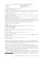
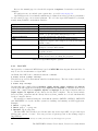
Accordingly, we offer different frontends into which you can log in for interactive access.
Besides the frontends for general use, there are frontends with special features: access to specific
hardware (Harpertown, Gainestown), graphical login (X-Win32 servers), or for performing big
data transfers.
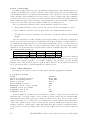
See table 1.1 on page 9.
Frontend name
cluster.rz.RWTH-Aachen.DE
cluster2.rz.RWTH-Aachen.DE
cluster-linux.rz.RWTH-Aachen.DE
OS
Linux
cluster-x.rz.RWTH-Aachen.DE
cluster-x2.rz.RWTH-Aachen.DE
cluster-copy.rz.RWTH-Aachen.DE
cluster-copy2.rz.RWTH-Aachen.DE
cluster-linux-nehalem.rz.RWTH-Aachen.DE
cluster-linux-xeon.rz.RWTH-Aachen.DE
Linux, for graphical login
(X-Win32 software)
Linux, for data transfers
Linux (Gainestown)
Linux (Harpertown)
Table 1.1: Frontend nodes
3
4
Note that three letter acronym “ITC” is not welcome.
see appendix B on page 110 for a quick introduction to the Linux cluster
The RWTH HPC-Cluster User's Guide, Version 8.3.0, March 2014
9
To improve the cluster’s operating stability, the frontend nodes are rebooted weekly, typically on Monday early in the morning. All the other machines are running in non-interactive
mode and can be used by means of batch jobs (see chapter 4.4 on page 35).
1.2
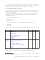
Development Software Overview
A variety of different development tools as well as other ISV5 software is available. However,
this primer focuses on describing the available software development tools. Recommended tools
are highlighted in bold blue.
An overview of the available compilers is given below. All compilers support serial programming as well as shared-memory parallelization (autoparallelization and OpenMP):
• Intel (F95/C/C++)
• Oracle Solaris Studio (F95/C/C++)
• GNU (F95/C/C++)
• PGI (F95/C/C++)
For Message Passing (MPI) one of the following implementations can be used:
• Open MPI
• Intel MPI
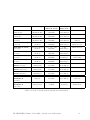
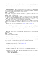
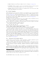
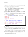
Table 1.2 on page 10 gives an overview of the available debugging and analyzing / tuning
tools.
Tool
Debugging
Ser
ShMem
MPI
TotalView
X
X
X
Allinea DDT
X
X
X
Oracle Thread Analyzer
Analysis
/ Tuning
X
Intel Inspector
GNU gdb
PGI pgdbg
X
X
X
Oracle Performance Analyzer
X
GNU gprof
X
Intel VTune Amplifier
X
X
X
X
Intel Trace Analyzer and Collector
X
Vampir
Scalasca
X
X
Table 1.2: Development Software Overview. Ser = Serial Programming; ShMem = Shared
memory parallelization: OpenMP or Autoparallelization; MPI=Message Passing
5
Independent Software Vendor.
aachen.de/display/CC/Installed+software
10
See
a
list
of
installed
products:
https://doc.itc.rwth-
The RWTH HPC-Cluster User's Guide, Version 8.3.0, March 2014
1.3
Examples
To demonstrate the various topics explained in this user’s guide, we offer a collection of example
programs and scripts.
The example scripts demonstrate the use of many tools and commands. Command lines,
for which an example script is available, have the following notation in this document:
$ $PSRC/pex/100|| echo “Hello World”
You can either run the script $PSRC/pex/100 to execute the example. The script includes all
necessary initializations. Or you can do the initialization yourself and then run the command
after the “pipes”, in this case echo “Hello World”. However, most of the scripts are offered
for Linux only.
The example programs, demonstrating e.g. the usage of parallelization paradigms like
OpenMP or MPI, are available on a shared cluster file system. The environment variable
$PSRC points to its base directory.
The code of the examples is usually available in the programming languages C++, C and
Fortran (F). The directory name contains the programming language, the parallelization
paradigm, and the name of the code, e.g. the directory $PSRC/C++-omp-pi contains the
Pi example written in C++ and parallelized with OpenMP. Available paradigms are:
• ser : Serial version, no parallelization. See chapter 5 on page 48
• aut : Automatic parallelization done by the compiler for shared memory systems. See
chapter 6.1 on page 65
• omp : Shared memory parallelization with OpenMP directives. See ch. 6.1 on page 65
• mpi : Parallelization using the message passing interface (MPI). See ch. 6.2 on page 72
• hyb : Hybrid parallelization, combining MPI and OpenMP. See ch. 6.3 on page 75
The example directories contain Makefiles for the “gmake” tool available on Linux.Furthermore,
there are some more specific examples in project subdirectories like vihps.
You have to copy the examples to a writeable directory before using them. You can copy
an example to your home directory by changing into the example directory with e.g.
$ cd $PSRC/F-omp-pi
and running
$ gmake cp
After the files have been copied to your home directory, a new shell is started and instructions
on how to build the example are given.
$ gmake
will invoke the compiler to build the example program and then run it.
Additionally, we offer a detailed beginners introduction for the Linux cluster as an appendix
(see chapter B on page 110). It contains a step-by-step description about how to build and run
a first program and should be a good starting point in helping you to understand many topics
explained in this document. It may also be interesting for advanced Linux users who are new
to our HPC-Cluster to get a quick start.
1.4
Further Information
Please check our web pages:
http://www.itc.rwth-aachen.de/hpc/
The latest version of this document is located here:
http://www.itc.rwth-aachen.de/hpc/primer/
The RWTH HPC-Cluster User's Guide, Version 8.3.0, March 2014
11
News, like new software or maintenance announcements about the HPC-Cluster, is provided
through the rzcluster mailing list. Interested users are invited to join this mailing list at
http://mailman.rwth-aachen.de/mailman/listinfo/rzcluster
The mailing list archive is accessible at
http://mailman.rwth-aachen.de/pipermail/rzcluster
Semi-annual, workshops on actual themes of HPC take place in Aachen:
http://www.itc.rwth-aachen.de/ppces/
http://www.itc.rwth-aachen.de/aixcelerate/
Please feel free to send feedback, questions or problem reports to
[email protected]
Have fun using the HPC-Cluster!
12
The RWTH HPC-Cluster User's Guide, Version 8.3.0, March 2014
2
Hardware
This chapter describes the hardware architecture of the various machines which are available
as part of the RWTH Aachen University’s HPC-Cluster.
2.1
Terms and Definitions
Since the concept of a processor has become increasingly unclear and confusing, it is necessary
to clarify and specify some terms.6 Previously, a processor socket was used to hold one processor
chip7 and appeared to the operating system as one logical processor. Today a processor socket
can hold more than one processor chip. Each chip usually has multiple cores. Each core may
support multiple threads simultaneously in hardware. It is not clear which of those should be
called a processor, and everybody has another opinion on that. Therefore we try to avoid the
term processor for hardware and will use the following more specific terms.
A processor socket is the foundation on the main board where a processor package 8 , as
delivered by the manufacturer, is installed. An 8-socket system, for example, contains up to 8
processor packages. All the logic inside of a processor package shares the connection to main
memory (RAM).
A processor chip is one piece of silicon, containing one or more processor cores. Although
typically only one chip is placed on a socket (processor package), it is possible that there is
more than one chip in a processor package (multi-chip package). A processor core is a standalone
processing unit, like the ones formerly known as “processor” or “CPU”. One of today’s cores
contains basically the same logic circuits as a CPU previously did. Because an n-core chip
consists, coarsely speaking, of n replicated “traditional processors”, such a chip is theoretically,
memory bandwidth limitations set aside, n times faster than a single-core processor, at least
when running a well-scaling parallel program. Several cores inside of one chip may share caches
or other resources.
A slightly different approach to offer better performance is hardware threads (Intel: Hyper
Threading ). Here, only parts of the circuits are replicated and other parts, usually the computational pipelines, are shared between threads. These threads run different instruction streams
in pseudo-parallel mode. The performance gained by this approach depends much on hardware
and software. Processor cores not supporting hardware threads can be viewed as having only
one thread.
From the operating system’s point of view every hardware thread is a logical processor . For
instance, a computer with 8 sockets, having installed dual-core processors with 2 hardware
threads per core, would appear as a 32 processor (“32-way ”) system.9 As it would be tedious
to write “logical processor” or “logical CPU” every time when referring to what the operating
system sees as a processor, we will abbreviate that.
Anyway, from the operating system’s or software’s point of view it does not make a difference
whether a multicore or multisocket system is installed.
2.1.1
Non-Uniform Memory Architecture (NUMA)
For performance considerations the architecture of the computer is crucial especially regarding
memory connections. All of today’s modern multiprocessors have a non-uniform memory access
(NUMA) architecture: parts of the main memory are directly attached to the processors.
Today, all common NUMA computers are actually cache-coherent NUMA (or ccNUMA)
ones: There is special-purpose hardware (or operating system software) to maintain the cache
coherence. Thus, the terms NUMA and ccNUMA are very often used as replacement for each
6
Unfortunately different vendors use the same terms with various meanings.
A chip is one piece of silicon, often called “die”.
8
Intel calls this a processor
9
The term “n-way” is used in different ways. For us, n is the number of logical processors which the operating
system sees.
7
The RWTH HPC-Cluster User's Guide, Version 8.3.0, March 2014
13
other. The future development in computer architectures can lead to a rise of non-cachecoherent NUMA systems. As far as we only have ccNUMA computers, we use ccNUMA and
NUMA terms interchangeably.
Each processor can thus directly access those memory banks that are attached to it (local
memory ), while accesses to memory banks attached to the other processors (remote memory )
will be routed over the system interconnect. Therefore, accesses to local memory are faster
than those to remote memory and the difference in speed may be significant. When a process
allocates some memory and writes data into it, the default policy is to put the data in memory
which is local to the processor first accessing it (first touch), as long as there is still such local
memory available.
To obtain the whole computing performance, the application’s data placement and memory
access pattern are crucial. Unfavorable access patterns may degrade the performance of an
application considerably. On NUMA computers, arrangements regarding data placement must
be done both by programming (accessing the memory the “right” way; see chapter 6.1.2 on
page 67) and by launching the application (Binding ,10 see chapter 3.1.1 on page 26).
2.2
Configuration of HPC-Cluster
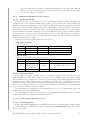
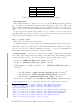
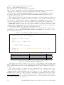
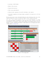
Table 2.3 on page 15 lists the nodes of the HPC-Cluster. The node names reflect the operating
system running. The list contains only machines which are dedicated to general usage. In
the course of the proceeding implementation of our Integrative Hosting concept (chapter 2.2.1
on page 14) there are a number of hosted machines that sometimes might be used for batch
production jobs. These machines can not be found in the list.
The IT Center’s part of the HPC-Cluster has an accumulated peak performance of about
325 TFlops. The in 2011 new installed part of the cluster reached rank 32 in the June 2011
Top500 list: http://www.top500.org/list/2011/06/100.
2.2.1
Integrative Hosting
The IT Center offers institutes of the RWTH Aachen University to integrate their computers
into the HPC-Cluster, where they will be maintained as part of the cluster. The computers will be installed in the IT Center’s computer room where cooling and power is provided.
Some institutes choose to share compute resources with others, thus being able to use more
machines when the demand is high and giving unused compute cycles to others. Further Information can be found at http://www.itc.rwth-aachen.de/go/id/esvg/ and https://doc.itc.rwthaachen.de/display/IH/Home
The hosted systems have an additional peak performance of about 40 TFlops.
2.3
The Intel Xeon based Machines
The Intel Xeon “Nehalem” and “Westmere” based Machines provide the main compute capacity
in the cluster. “Nehalem” and “Westmere” are generic names, so different (but related) processors types are available. These processors support a wide variety of x86-instruction-extensions
up to SSE4.2, nominal clock speed vary from 1.86 GHz to 3.6 GHz, most types can run more
than one thread per core (hyperthreading).
“Sandy Bridge” is the codename for a microarchitecture developed by Intel to replace the
Nehalem family (Nehalem and Wesmere) of cores. The “Sandy Bridge” CPUs are produced
in 32 nm process. The unique feature of the “Sandy Bridge” CPUs is the availability of the
Advanced Vector Extensions (AVX) 11 vectors units with 256-bit instruction set.
10
Processor/Thread Binding means explicitly enforcing processes or threads to run on certain processor cores,
thus preventing the OS scheduler from moving them around.
11
http://software.intel.com/en-us/intel-isa-extensions, http://en.wikipedia.org/wiki/Advanced_Vector_Extensions
14
The RWTH HPC-Cluster User's Guide, Version 8.3.0, March 2014
Model
Processor type
Sockets/Cores
/Threads (total)
Memory
Flops/node
Hostname
Bull MPI-S
(1098 nodes)
Bull MPI-L
(252 nodes)
Bull MPI-D
(8 nodes)
Bull SMP-S (BCS)
(67 nodes)
Bull SMP-L (BCS)
(15 nodes)
Bull SMP-XL (BCS)
(2 nodes)
Bull SMP-D (BCS)
(2 nodes)
Intel Xeon X5675
“Westmere EP”
Intel Xeon X5675
“Westmere EP”
Intel Xeon X5675
“Westmere EP”
Intel Xeon X7550
“Beckton”
Intel Xeon X7550
“Beckton”
Intel Xeon X7550
“Beckton”
Intel Xeon X7550
“Beckton”
2 / 12 / 24
3.06 GHz
2 / 12 / 24
3.06 GHz
2 / 12 / 24
3.06 GHz
4x4 / 128 / 128
2.00 GHz
4x4 / 128 / 128
2.00 GHz
4x4 / 128 / 128
2.00 GHz
2x4 / 64 / 64
2.00 GHz
24 GB
146.88 GFlops
96 GB
146.88 GFlops
96 GB
146.88 GFlops
256 GB
1024 GFlops
1 TB
1024 GFlops
2 TB
1024 GFlops
256 GB
512 GFlops
linuxbmc0253..1350
Bull/ScaleMP
(1 node)
Intel Xeon X7550
“Beckton”
64 / 512 / 1024
2.00 GHz
4 TB
4096 GFlops
linuxscalec3
Sun Fire
X4170 (8 nodes)
Sun Blade
X6275 (192 nodes)
Sun Fire
X4450 (10 nodes)
Intel Xeon X5570
“Gainestown”
Intel Xeon X5570
“Gainestown”
Intel Xeon 7460
“Dunnington”
2 / 8 / 16
2.93 GHz
2 / 8 / 16
2.93 GHz
4 / 24 / 2.66 GHz
36 GB
93.76 GFlops
24 GB
93.76 GFlops
128-256 GB
255.4 GFlops
linuxnc001..008
Fujitsu-Siemens
RX600S4/X
(2 nodes)
Fujitsu-Siemens
RX200S4/X
(60 nodes)
Intel Xeon X7350
“Tigerton”
4 / 16 / 2.93 GHz
64 GB
187.5 GFlops
cluster2
cluster-x2
Intel Xeon E5450
“Harpertown”
2/8/3.0 GHz
16 - 32 GB
96 GFlops
cluster-linux-xeon
winhtc04..62
linuxbmc0001..0252
linuxbdc01..07
cluster-x
linuxbcsc01..63
linuxbcsc83..86
linuxbcsc68..82
linuxbcsc64,65
cluster
cluster-linux
linuxnc009..200
linuxdc01..09
Table 2.3: Node overview (hosted systems are not included)
The RWTH HPC-Cluster User's Guide, Version 8.3.0, March 2014
15
2.3.1
The Xeon X5570 “Gainestown” (“Nehalem EP”) Processor
The Intel Xeon X5570 processors (codename “Gainestown”, formerly also “Nehalem EP”) are
quadcore processors where each core can run two hardware threads (hyperthreading). Each
core has a L1 and a L2 cache and all cores share one L3 cache.
• Level 1 (on chip): 32 KB data cache + 32 KB instruction cache (8-way associative)
• Level 2 (on chip): 256 KB cache for data and instructions (8-way associative)
• Level 3 (on chip): 8 MB cache for data and instructions shared between all cores (16-way
associative)
The cores have a nominal clock speed of 2.93 GHz.
2.3.2
The Xeon X7550 “Beckton” (“Nehalem EX”) Processor
Intel's Xeon X7550 Processors (codename “Beckton”, formerly also “Nehalem EX”) have eight
cores per chip. Each core is able to run two hyperthreads simultaneously. Each of these cores
has two levels of cache per core and one level 3 cache shared between all cores.
• Level 1 (on chip): 32 KB data cache + 32 KB instruction cache (8-way associative)
• Level 2 (on chip): 256 KB cache for data and instructions (8-way associative)
• Level 3 (on chip): 18 MB cache for data and instructions shared between all cores (16-way
associative)
The cores have a nominal clock speed of 2.00 GHz.
2.3.3
The Xeon X5675 “Westmere EP” Processor
The “Westmere” (formerly “Nehalem-C”) CPUs are produced in 32 nm process instead of 45 nm
process used for older Nehalems. This die shrink of Nehalem offers lower energy consumption
and a bigger number of cores.
Each processor has six cores. With Intel's Hyperthreading technology each core is able
to execute two hardware threads. The cache hierarchy is the same as for the other Nehalem
processors beside the fact that the L3 cache is 12MB in size and the nominal clock speed is
3.00 GHz.
• Level 1 (on chip): 32 KB data cache + 32 KB instruction cache (8-way associative)
• Level 2 (on chip): 256 KB cache for data and instructions (8-way associative)
• Level 3 (on chip): 12 MB cache for data and instructions shared between all cores (16-way
associative)
2.3.4
The Xeon E5-2650 “Sandy Bridge” Processor
Xeon E5-2650 is one of early-available “Sandy Bridge” server CPUs. Each processor has eight
cores. With Intel's Hyperthreading technology each core is able to execute two hardware
threads. The nominal clock speed is 2.00 GHz.12 The cache hierarchy is the same as for the
Nehalem processors beside the fact that the L3 cache is 20MB in size.
• Level 1 (on chip): 32 KB data cache + 32 KB instruction cache (8-way associative)
12
using Intel Turbo Boost up to 2.8 GHz, http://www.intel.com/content/www/us/en/architecture-andtechnology/turbo-boost/turbo-boost-technology.html
16
The RWTH HPC-Cluster User's Guide, Version 8.3.0, March 2014
• Level 2 (on chip): 256 KB cache for data and instructions (8-way associative)
• Level 3 (on chip): 20 MB cache for data and instructions shared between all cores (16-way
associative)
2.3.5
Memory
Each processor package (Intel just calls it processor) has its own memory controller and is
connected to a local part of the main memory. The processors can access the remote memory
via Intel's new interconnect called “Quick Path Interconnect”. So these machines are the first
Intel processor-based machines that build a ccNUMA architecture.
On ccNUMA computers, processor binding and memory placement are important to reach
the whole available performance (see chapter 2.1.1 on page 13 for details).
The machines are equipped with DDR3 RAM, please refer to table 2.3 on page 15 for
details. The total memory bandwidth is about 37 GB/s.
2.3.6
Network
The nodes are connected via Gigabit Ethernet and also via quad data rate (QDR) InfiniBand.
This QDR InfiniBand achieves an MPI bandwidth of 2.8 GB/s and has a latency of only 2 µs.
2.3.7
Big SMP (BCS) Systems
The nodes in the SMP complex are coupled to big shared memory systems with the proprietary
BCS (Bull Coherent Switch) chips. This means that 2 or 4 physical nodes ("boards") form a
8-socket or rather a 16-socket systems with up to 128 cores13 in one single system.
For the performance of shared memory jobs it is important to notice that not only the
BCS interconnect imposes a NUMA topology consisting of the four nodes, but still every node
consists of four NUMA nodes connected via the QPI, thus this system exhibits two different
levels of NUMAness.
2.3.8
ScaleMP System
The company ScaleMP14 provides software called vSMP foundation to couple several standard
x86 based servers into a virtual shared memory system. The software works underneath the
operating system, so that a standard Linux is presented to the user. Executables for x86 based
machines can run on the ScaleMP machines without recompilation or relinking.
Our installation couples 16 boards, each equipped with 4 Intel Xeon X7550 processors and
64 GB of main memory. So, a user sees a Single System Image on this machine with 512 Cores
and 3.7 TB of main memory. A part of physically availabe memory is used for system purposes
and thus is not availale for computing.
For the performance of shared memory jobs it is very important to notice that the ScaleMP
system exhibits two different levels of NUMAness, where the NUMA ratio between onboard
and offboard memory transfers is very high.
Please read carefully and take note of the End User License Agreement (EULA):
http://www.scalemp.com/eula
2.4
Special Systems: GPU-Cluster
The GPU-cluster comprises 30 nodes each with two GPUs, and one head node with one GPU.
In detail, there are 57 NVIDIA Quadro 6000 (Fermi) and 4 NVIDIA K20x (Kepler) GPUs.
Furthermore, each node is a two socket Intel Xeon “Westmere” EP (X5650) or “Sandy Bridge”
13
14
On Bull’s advise the Hyperthreading is OFF on all BCS systems.
http://www.scalemp.com/
The RWTH HPC-Cluster User's Guide, Version 8.3.0, March 2014
17
EP (E5-2650) server which contains a total of 12 or 16 cores running at 2.7 or 2.0 GHz and 24GB
or 64GB DDR3 memory. All nodes are conntected by QDR InfiniBand. The head node and
24 of the double-GPU nodes are used on weekdays (at daytime) for interactive visualizations
by the Virtual Reality Group15 of the IT Center. During the nighttime and on weekends, they
are available for GPU compute batch jobs. The remaining nodes enable, on the one hand,
GPU batch computing all-day and, on the other hand, interactive access to GPU hardware to
prepare the GPU compute batch jobs and to test and debug GPU applications.
The software environment on the GPU-cluster is now as similar as possible to the one on the
RWTH HPC-Cluster. GPU-related software (like NVIDIA’s CUDA Toolkit, PGI’s Accelerator
Model or a CUDA debugger) is additionally provided.
2.4.1
Access to the GPU cluster
2.4.1.1 Access
To get access to the system, your account has to be first authorized. If you are interested in
using GPUs, please write an to [email protected] with your user ID and let us
know that you want to use the GPU cluster.
2.4.1.2 Friendly Usage
All GPUs are in the exclusive process compute mode, which means that whenever a GPU
program is run it gets the whole GPU and does not have to compete with other programs
for resources (e.g. GPU memory). Furthermore, it enables several threads in a single process
to use both GPUs that are available on each node (cf. e.g. cudaSetDevice) instead of being
restricted to one thread per device. Therefore you should use them reasonably. Please run
long computations in batch mode only and close any debuggers after usage. We also appreciate
compute jobs that allow other users to run their jobs once in a while. Thank you!
2.4.1.3 Interactive Mode
You can access the GPU nodes interactively via SSH. If needed, you can also first log into
one of our (graphical) frontends and then use SSH to log into one of the interactive GPU nodes.
GPU login nodes are listed in the chapter 2.4.4 on page 21.
Be aware that we have special time windows for certain GPU nodes. The time frames for
interactives access are also listed in the chapter 2.4.4 on page 21.
2.4.1.4 GPU + MPI
If you would like to test your GPU + MPI program interactively, you can do so on the dialog
nodes using our mpiexec wrapper $MPIEXEC (see chapter 6.2.1 on page 72). To get your MPI
program run on the GPU machines, you have to explicitly specify their hostnames, otherwise
your program will get started on the regular MPI backend which does not have any GPUs.
You can do so by providing the following option:
-H host1,host2,host3
However, you should not use this option with regular MPI machines! You can also provide
how many processes shall be run on a host by host basis (see the example below or call $MPIEXEC
-help). Furthermore, it could be useful to simply specify the same number of processes to be
run on all hosts (e.g. if each of your processes uses one GPU). For our interactive mpiexec
wrapper use the -m ppn option where ppn is the desired number of processes per node.
Example with 2 processes on each host:
$ $MPIEXEC -np 4 -m 2 -H linuxgpud1,linuxgpud2 foobar.exe
Example with 1 process on the first host, 3 processes on the second:
$ $MPIEXEC -np 4 -H linuxgpud1:1,linuxgpud2:3 foobar.exe
15
18
http://www.itc.rwth-aachen.de/vr
The RWTH HPC-Cluster User's Guide, Version 8.3.0, March 2014
2.4.2
GPU Programming Models
2.4.2.1 CUDA
NVIDIA provides the CUDA C SDK for programming their GPUs. PGI added a
CUDA Fortran version, also for NVIDIA GPUs. On the GPU cluster, we recommend that
the most-recent CUDA Toolkit Version (module load cuda) is used. For compatibility we also
provide older versions of the toolkit (module avail cuda). Usage information can be found
online.16
2.4.2.2 OpenCL
OpenCL is an open standard for programming GPUs, CPUs (NVIDIA, AMD, Intel,...) and
other device using a C-like API. Usage information can be found online.17
2.4.2.3 OpenACC
OpenACC is an industry standard for directive-based programming of accelerators. PGI,
Cray and Caps support OpenACC in their commercial compilers. The PGI compiler installed
on the cluster can be used to develop OpenACC codes. Usage information can be found
online.18
2.4.2.4 NVIDIA GPU Computing SDK
NVIDIA provides numerous examples in CUDA C (and OpenCL C). See online19 on how to
get and use them.
2.4.3
GPU Batch Mode
Information about the general usage of LSF can be found in chapter 4.4.1 on page 35.
You can use the bsub command to submit jobs:
$ bsub [options] command [arguments]
We advise you to use a batch script in which the #BSUB magic cookie can be used to
specify job requirements:
$ bsub < gpuDeviceQueryLsf.sh
You can submit batch jobs for the GPU cluster at any time. However, dependent on the
batch mode availability, scheduling and occupancy, it might take a while until your compute
job finishes (see chapter 2.4.4 on page 21).
In the following, we differentiate between short test runs on the one hand and real program
runs on the other hand.
2.4.3.1 Short test runs (daytime)
Short test runs can be done on a couple of machines which are in batch mode also during
daytime. If you would like to test your batch script, add the following:
#BSUB -a gpu
If you would also like to use MPI, you can combine the requests for using GPU and MPI
(please see below for more details on the usage of MPI):
#BSUB -a "gpu openmpi"
2.4.3.2 Long runs (nighttime, weekend)
Production jobs (i.e. longer runs or performance tests) have to be scheduled on the GPU
cluster (nighttime and weekends). Therefore, you have to select the appropriate queue:
#BSUB -q gpu
16
https://doc.itc.rwth-aachen.de/display/CC/CUDA
https://doc.itc.rwth-aachen.de/display/CC/OpenCL
18
https://doc.itc.rwth-aachen.de/display/CC/OpenACC
19
https://doc.itc.rwth-aachen.de/display/CC/NVIDIA+GPU+Computing+SDK
17
The RWTH HPC-Cluster User's Guide, Version 8.3.0, March 2014
19
You can either put the -q gpu option in your batch script file or give it to the bsub
command. You will get all requested machines exclusively. BTW: If you accidentally combine
-a gpu AND -q gpu, the -q gpu option takes precedence and your job will run during the
night on the GPU cluster.
2.4.3.3 Selecting a certain GPU type (Fermi/Kepler)
Since October 2013 there are nodes with two different kinds of GPUs in the cluster. If you
do not specify a certain kind, you will get an arbitrary GPU node. That is advantageous if
you are not dependent on a certain GPU type because you will get any node that is available
(so possibly less waiting time for the job).
If you need a certain GPU type, you have to request it in you batch script with either
#BSUB -R fermi
or
#BSUB -R kepler
Please note that in batch mode all (correct working) GPU machines are available, including
one node with only one GPU attached (linuxgpum1). If you would like to exclude this particular
node from your hostlist (e.g. due to the fact that you want to use 2 processes per node and
each process uses one GPU), please specify additionally the following (so that you will only get
machines that have two GPUs):
#BSUB -m bull-gpu-om
A combination of a certain GPU type with a certain number of GPUs, i.e. Fermi nodes
with two GPUs per node, could be requested as well:
#BSUB -R fermi
#BSUB -m bull-gpu-om
2.4.3.4 Example Scripts
In order to save some trees the example scripts are not included in this document. The
example scripts are available on the HPC-Cluster in the $PSRC/pis/LSF/ directory and online
at https://doc.itc.rwth-aachen.de/display/CC/GPU+batch+mode.
• Simple GPU Example - Run deviceQuery (from NVIDIA SDK) on one device:
$PSRC/pis/LSF/gpuDeviceQueryLsf.sh or Docuweb20
• MPI GPU Example - Run deviceQuery (not a real MPI application!) on 4 nodes (use
one device on each: $PSRC/pis/LSF/gpuMPIExampleLsf.sh or Docuweb21
Since we do not have requestable GPU slots in LSF at the moment, you have to explicitly
specify how many processes you would like to have per node (see ptile in the script file). This
is usually one or two, depending on how you would like to use the GPUs and how many GPUs
you would like to use per node. Examples:
• 1 process per node (ppn):
– If you would like to use only one GPU per node;
– If your process uses both GPUs at the same time, e.g. via cudaSetDevice.
• 2 processes per node (ppn):
– If each process communicates to a single GPU.
• More than 2 processes per node:
20
21
20
https://doc.itc.rwth-aachen.de/display/CC/GPU+batch+mode#GPUbatchmode-GPUSimple
https://doc.itc.rwth-aachen.de/display/CC/GPU+batch+mode#GPUbatchmode-GPUMPI
The RWTH HPC-Cluster User's Guide, Version 8.3.0, March 2014
– If you also have processes that do computation on the CPU only. Be aware that our
GPUs are set to "exclusive process" mode, which is the reason why no more than
one process could use each GPU.
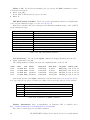
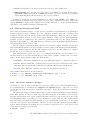
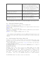
2.4.4
Limitations Within the GPU Cluster
2.4.4.1 Operation modes
The 24 render nodes (+ head node) are used on weekdays (during daytime) for interactive
visualizations by the Virtual Reality Group (VR) of IT Centerand are NOT available for
GPGPU computations during that period. However, during the night and during the weekends
they can be used for GPU compute batch jobs. Furthermore, few nodes run in batch mode
the whole day long (see below) for the purpose of executing short batch jobs (e.g. for testing).
Several dialogue nodes enable interactive access to the GPU hardware. There the GPU compute
batch jobs can be prepared and GPU applications can be tested and debugged. A couple of
dialogue nodes (see below) stay in interactive mode the whole day. The others are switched to
batch mode during the evening.
Between every mode switch each system is rebooted.
• Interactive Mode
dialogue nodes
#nodes node names
1
linuxgpud1
2
linuxgpud[2-3]
1
linuxnvc01
GPU type
Fermi
Fermi
Kepler
operating time
whole day [24/7]
working days: 7:40 am - 8 pm
whole day [24/7]
• Batch Mode
all nodes (excluding linuxgpud1, linuxnvc01)
#nodes
node names
GPU type
operating time
1
linuxgpud4
Fermi
whole day (short test runs only!)
linuxgpud[2-3]
working days: 8 pm - 7:30 am
27
linuxgpus[01-24]
Fermi
weekends: whole day
linuxgpum1
1
linuxnvc02
Kepler
whole day (short test runs only!)
2.4.4.2 Exclusive Mode
As the GPUs are set to “exclusive” mode, you will get an error message if you try to run
your program on a GPU device that is already in use by another user. If possible, simply
choose another device number for execution of your program. For CUDA applications do not
explicitly set the device number in your program (e.g. with a call to cudaSetDevice) if not
strictly necessary. Then your program will automatically use any available GPU device (if
there is one). However, if you set a specific device number, you will have to wait until that
device becomes available (and try it again).
Keep in mind that debugging sessions always run on device 0 (default) and therefore you
might exhibit the same problem there.
If you would like to run on a certain GPU (e.g. debugging a non-default device), you may
mask certain GPUs by setting a environment variable:
$ export CUDA_VISIBLE_DEVICES=<GPU ID>
2.4.4.3 X Configuration
We have different X configurations on different GPU nodes. This may impact your programs
in certain situations. To find out about the current setup use nvidia-smi and look for “Disp.
On” or “Disp. Off ”.
The RWTH HPC-Cluster User's Guide, Version 8.3.0, March 2014
21
Current settings:
• Login nodes: An X session runs on the display of GPU 1.
On GPU 0 is the display mode disabled.
• Batch nodes: Display mode is disabled on both GPUs
2.5
Special Systems: Intel Xeon Phi Cluster
Note: For latest info take a look at this wiki:
https://doc.itc.rwth-aachen.de/display/CC/Intel+Xeon+Phi+cluster
The Intel Xeon Phi Cluster comprises 9 nodes each with two Intel Xeon Phi coprocessors
(MIC). One of these nodes is used as frontend and the other 8 nodes run in batch mode. More
specifically, each node consists of two 60-core MICs running at 1.05 GHz with 8 GB of memory
each and two 8-core Intel Xeon E5-2650 (codename Sandy Bridge) CPUs running at 2.0 GHz
with 32 GB of main memory.
2.5.1
Access to the Intel Xeon Phi cluster
2.5.1.1 Access To get access to this system your account has to be authorized first. If you
are interested in using the machine, please write to [email protected] with your
user ID and let us know that you would like to use the Intel Xeon Phi cluster.
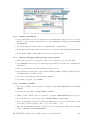
2.5.1.2 Interactive Mode The frontend system can be used interactively. It should only
be used for programming, debugging, preparation and post-processing of batch jobs. It is not
allowed to run production jobs on it.
Login from Linux is possible via Secure Shell (ssh). For example:
$ ssh cluster-phi.rz.rwth-aachen.de
From the frontend you can then login to the coprocessors:
$ ssh cluster-phi-mic0
or
$ ssh cluster-phi-mic1
Please note that the host system cluster-phi is only accessible from our normal dialog systems, therefore you should first log into one of them and then use SSH to log into cluster-phi.
The coprocessors are only accessible from their host system.
Like every other frontend system in the HPC-Cluster, cluster-phi is rebooted every Monday at 6 am.
Registered users can access their $HOME and $WORK directories at the coprocessors under
/home/<userid> and /work/<userid>.
Due to the fact that programs using the Intel Language Extension for Offload (LEO) are
started under a special user ID (micuser), file IO within an offloaded region is not allowed.
2.5.2
Programming Models
Three different programming models can be used. Most programs can run natively on the
coprocessor. Also, parallel regions of the code can be offloaded using the Intel Language Extension for Offload (LEO). Finally, Intel MPI can be used to send messages between processes
running on the hosts and on the coprocessors.
2.5.2.1 Native Execution
Cross-compiled programs using OpenMP, Intel Threading Building Blocks (TBB) or Intel
Cilk Plus can run natively on the coprocessor.
22
The RWTH HPC-Cluster User's Guide, Version 8.3.0, March 2014
To prepare an application for native execution, the Intel compiler on the host must be
instructed to cross-compile the application for the coprocessor (e.g. by adding the -mmic
switch to your makefile). Once the program executable is properly built, you can log into the
coprocessor and start the program in the normal way, e.g.:
$ ssh cluster-phi-mic1
$ cd /path/to/dir
$ ./a.out
The ld_library_path and the path environment variables will be set automatically.
2.5.2.2 Language Extension for Offload (LEO)
The Intel Language Extension for Offload offers a set of pragmas and keywords that can be
used to tag code regions for execution on the coprocessor. Programmers have additional control
over data transfer by clauses that can be added to the offload pragmas. One advantage of the
LEO model compared to other offload programming models is that the code inside the offloaded
region may contain arbitrary code and is not restricted to certain types of constructs. The code
may contain any number of function calls and it can also use any parallel programming model
supported (e.g. OpenMP, Fortran’s do concurrent, POSIX Threads, Intel TBB, Intel Cilk
Plus).
2.5.2.3 MPI
An MPI program with host-only ranks may employ LEO in order to utilize the performance
of the coprocessors. An MPI program may also run in native mode with ranks on both the
processors and the coprocessors. That way MPI can be used for reduction of the parallel layers.
To compile an MPI program on the host, the MPI module must be switched:
$ module switch openmpi intelmpi/4.1mic
The module defines the following variables:
I_MPI_MIC=enable
I_MPI_MIC_POSTFIX=.mic
After that two different versions of the executable must be build. One with the -mmic
switch and an added .mic suffix to the name of the executable file and one without:
$ $MPICC micproc.c -o micproc
$ $MPICC micproc.c -o micproc.mic -mmic
In order to start MPI applications over multiple MICs, the interactive $MPIEXEC wrapper
can be used. The wrapper is only allowed to start processes on MICs when you are logged in
on a MIC-enabled host, e.g. cluster-phi.rz.rwth-aachen.de.
The mpiexec wrapper can be used as usual with dynamic load balancing. In order to
distinguish between processes on the host and processes on the MICs, there are 2 different
command line parameters, shown in the following examples.
Start 2 processes on the host:
$ $MPIEXEC -nph 2 micproc
Start 2 processes on the coprocessors:
$ $MPIEXEC -npm 2 micproc.mic
The parameters can also be used simultaneously like:
$ $MPIEXEC -nh 2 -nm 30 micproc
Also there is the option to start MPI application on coprocessors and hosts without the
load balancing. The value for each host defines the number of processes on this host, NOT the
compute slots.
16 processes on the host and 10 processes spanning both coprocessors:
$ $MPIEXEC -H cluster-phi:16,cluster-phi-mic0:10,cluster-phi-mic1:10 <exec>
The RWTH HPC-Cluster User's Guide, Version 8.3.0, March 2014
23
2.5.2.4 Batch Mode
Information about the general usage of LSF can be found in chapter 4.4.1 on page 35. You
can use the bsub command to submit jobs:
$ bsub [options] command [arguments]
We advise you to use a batch script in which the #BSUB magic cookie can be used to
specify job requirements:
$ bsub < jobscript.sh
Please note that the coprocessor(s) will be rebooted for every batch job, therefore it could
take some time before your application starts and you can see any output from bpeek. For
general information on job submission please refer to chapter 4.4.1 on page 35.
To submit a job for the Intel Xeon Phi's you have to put
#BSUB -a phi
in your submission script. Furthermore, you have to specify a special job description parameter
that determines the job type (offload (LEO), native or MPI job):
• For Language Extension for Offload (LEO), put
#BSUB -Jd "leo=a;b"
where:
– a is the number of MICs
– b is the number of threads on the MICs
• For native job use
#BSUB -Jd "native"
• For MPI specify
#BSUB -Jd "hosts=a;b;mics=c;d""
where:
– a is the number of hosts
– b is a comma separated list of MPI processes on the hosts
– c is the number of MICs
– d is a comma separated list of MPI processes on the MICs
2.5.2.5 Example Scripts
In order to save some trees the example scripts are not included in this document. The
example scripts are available on the HPC-Cluster in the $PSRC/pis/LSF/ directory and online
at https://doc.itc.rwth-aachen.de/display/CC/Batch+mode.
• LEO (Offload) Job - $PSRC/pis/LSF/phi_leo.sh or Docuweb22
• MPI Job - $PSRC/pis/LSF/phi_mpi.sh or Docuweb23
• Native Job - $PSRC/pis/LSF/phi_native.sh or Docuweb24
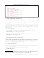
2.5.2.6 Special MPI Job Configurations
If you would like to run all your processes on the MICs only please follow the next example.
It shows how to use two MICs with 20 processes on each of them:
22
https://doc.itc.rwth-aachen.de/display/CC/Batch+mode#Batchmode-LEO(Offload)Job
https://doc.itc.rwth-aachen.de/display/CC/Batch+mode#Batchmode-MPIJob
24
https://doc.itc.rwth-aachen.de/display/CC/Batch+mode#Batchmode-NativeJob
23
24
The RWTH HPC-Cluster User's Guide, Version 8.3.0, March 2014
...
### The number of compute slots must be >= the number of hosts
#BSUB -n 1
...
### Now specify the type of Phi job:
### "hosts" -> MPI-Job
### "hosts=a;b;mics=c;d"
###
a: number of hosts
###
b: comma separated list of MPI processes on the ordered hosts
###
!!! you can even specify a "0" for each host !!!
###
c: number of MICs
###
d: comma separated list of MPI processes on the ordered MICs
#BSUB -Jd "hosts=1;0;mics=2;20,20"
...
You have to reserve the hosts and each host needs at least one process, otherwise the job will
not start.
2.5.2.7 Limitations
The Intel Xeon Phi cluster is running in the context of our innovative computing initiative,
which means that we do not guarantee its availability. At the moment the following limitations
are in place:
• There is no module system at the coprocessors.
• Only one compiler version (always the default Intel compiler) and one MPI version (intelmpi/*mic) are supported.
• Intel MPI: LSF does not terminate the job after your MPI application has finished. Please
use a small run time limit (#BSUB -W) in order to prevent resources from being blocked
for extended periods of time. The job will terminate after reaching that limit.
• LEO is not supported in MPI jobs.
• Our mpi_bind script (see chapter 4.4.1 on page 42) does not work for jobs on the Intel
Xeon Phi. Please refer to the Intel MPI manual for details on how to enable process
binding/pinning.
2.5.2.8 Further Information
Introduction to the Intel Xeon Phi in the RWTH Compute Cluster Environment, 2013-08-07:
Slides,25 Exercises.26
25
https://sharepoint.campus.rwth-aachen.de/units/rz/HPC/public/
Shared Documents/2013-08-07_mic_tutorial.pdf
26
https://sharepoint.campus.rwth-aachen.de/units/rz/HPC/public/
Shared Documents/2013-08-07_ex_phi.tar.gz
The RWTH HPC-Cluster User's Guide, Version 8.3.0, March 2014
25
3
Operating Systems
To accommodate our user's needs we are running two different operating systems on the machines of the HPC-Cluster at the RWTH Aachen University: Linux (see chapter 3.1 on page
26) and Windows (not described in this document).
3.1
Linux
Linux is a UNIX-like operating system. We are running the 64-bit version of Scientific Linux
(SL), with support for 32-bit binaries, on our systems. Scientific Linux is a binary-compatible
clone of RedHat Enterprise Linux (RHEL).
The Scientific Linux release is displayed by the command:
$ cat /etc/issue
The Linux kernel version can be printed with the command
$ uname -r
3.1.1
Processor Binding
Note: The usage of user-defined binding may destroy the performance of other jobs running
on the same machine. Thus, the usage of user-defined binding is only allowed in batch mode,
if cluster nodes are reserved exclusively. Feel free to contact us if you need help with binding
issues.
During the runtime of a program, it could happen (and it is most likely) that the scheduler
of the operating system decides to move a process or thread from one CPU to another in order
to try to improve the load balance among all CPUs of a single node. The higher the system
load is, the higher is the probability of processes or threads moving around. In an optimal
case this should not happen because, according to our batch job scheduling strategy, the batch
job scheduler takes care not to overload the nodes. Nevertheless, operating systems sometimes
do not schedule processors in an optimal manner for HPC applications. This may decrease
performance considerably because cache contents may be lost and pages may reside on a remote
memory location where they have been first touched. This is particularly disadvantageous on
NUMA systems because it is very likely that after several movement many of the data accesses
will be remote, thus incurring higher latency. Processor Binding means that a user explicitly
enforces processes or threads to run on certain processor cores, thus preventing the OS scheduler
from moving them around.
On Linux you can restrict the set of processors on which the operating system scheduler
may run a certain process (in other words, the process is bound to those processors). This
property is called the CPU affinity of a process. The command taskset allows you to specify
the CPU affinity of a process prior to its launch and also to change the CPU affinity of a
running process.
You can get the list of available processors on a system by entering
$ cat /proc/cpuinfo
The following examples show the usage of taskset. We use the more convenient option -c to
set the affinity with a CPU list (e.g. 0,5,7,9-11) instead of the old-style bitmasks.
$ $PSRC/pex/321|| taskset -c 0,3 a.out
You can also retrieve the CPU affinity of an existing task:
$ taskset -c -p pid
Or set it for a running program:
$ taskset -c -p list pid
Note that the Linux scheduler also supports natural CPU affinity: the scheduler attempts
26
The RWTH HPC-Cluster User's Guide, Version 8.3.0, March 2014
to keep processes on the same CPU as long as this seems beneficial for system performance.
Therefore, enforcing a specific CPU affinity is useful only in certain situations.
If using the Intel compilers with OpenMP programs, processor binding of the threads can
also be done with the kmp_affinity environment variable (see chapter 6.1.3 on page 67).
Similar environment variables for the Oracle compiler are described in section 6.1.4 on page 68
and for the GCC compiler in section 6.1.5 on page 70.
The MPI vendors also offer binding functionality in their MPI implementations; please refer
to the documentation.
Furthermore we offer the R_Lib library. It contains portable functions to bind processes
and threads (see 9.8 on page 98 for detailed information).
3.2
Addressing Modes
Programs can be compiled and linked either in 32-bit mode or in 64-bit mode. This affects
memory addressing, the usage of 32- or 64-bit pointers, but has no influence on the capacity or
precision of floating point numbers (4- or 8-byte real numbers). Programs requiring more than
4 GB of memory have to use the 64-bit addressing mode. You have to specify the addressing
mode at compile and link27 time. On Linux the default mode is 64-bit.
Note: long int data and pointers in C/C++ programs are stored with 8 bytes when using
64-bit addressing mode, thus being able to hold larger numbers. The example program shown
below in listing 1 on page 27 prints out “4” twice in the 32-bit mode:
$ $CC $FLAGS_ARCH32 $PSRC/pis/addressingModes.c; ./a.out
and “8” twice in the 64-bit mode:
$ $CC $FLAGS_ARCH64 $PSRC/pis/addressingModes.c; ./a.out
Listing 1: Show length of pointers and long integer variables
1
2
3
4
5
6
7
8
9
10
# include < stdio .h >
int main ( int argc , char ** argv )
{
int * p ;
long int li ;
printf ( " % lu % lu \ n " ,
( unsigned long int ) sizeof ( p ) ,
( unsigned long int ) sizeof ( li ));
return 0;
}
27
Note the environment variables $FLAGS_ARCH64 and $FLAGS_ARCH32 which are set for compilers
by the module system (see chapter 5.2 on page 48).
The RWTH HPC-Cluster User's Guide, Version 8.3.0, March 2014
27
4
The RWTH Environment
4.1
4.1.1
Login to Linux
Command line Login
The secure shell ssh is used to log into the Linux systems. Usually ssh is installed by default
on Linux and Unix systems. Therefore you can log into the cluster from a local 28 Unix or
Linux machine using the command
$ ssh -l username cluster.rz.rwth-aachen.de
For data transfers use the scp command.
A list of frontend nodes you can log into is given in table 1.1 on page 9.
To log into the Linux cluster from a Windows machine, you need to have an SSH client
installed. Such a client is provided for example by the cygwin (http://www.cygwin.com) environment, which is free to use. Other software is available under different licenses, for example
PuTTY (http://www.chiark.greenend.org.uk/~sgtatham/putty/download.html) or SSH Client
for Windows (ftp://ftp.cert.dfn.de/pub/tools/net/ssh).
The SSH Client for Windows provides a graphical file manager for copying files to and from
the cluster as well (see chapter 4.2.1 on page 31); another tool providing such functionality is
WinSCP (http://winscp.net/eng/docs/start).
If you log in over a weak network connection you are welcome to use the screen program,
which is a full-screen CLI window manager. Even if the connection breaks down, your session
will be still alive and you will be able to reconnect to it after you logged in again.29
4.1.2
Graphical Login
If you need graphical user interface (GUI), you can use the X Window System.30 The
forwarding of GUI windows using the X Window System is possible when logged in in any
Linux frontend(see table 1.1 on page 9).
When logging from Linux or Unix you usually do not need to install additional packages.
Depending on your local configuration it may be necessary to use the -X31 flag of the ssh
command to enable the forwarding of graphical programs.
On Windows, to enable the forwarding of graphical programs a X server on your local
computer must run, e.g. the cygwin http://www.cygwin.com/ contains one. Another X
server for Windows is Xming: http://sourceforge.net/projects/xming/
However, the X Window System can be quite slow over weak network connection, and in
case of a temporary netwofk failure your program will die and the session is lost. In order
to prevent this we offer special frontends capable to run the X-Win32 software (see table
1.1 on page 9). These sofware packages allow you to run remote X11 sessions even across
low-bandwidth network connections, as well as reconnecting to running sessions.
4.1.2.1 X-Win32
The X-Win32 from StarNet Communications http://www.starnet.com/ is commercial software. However, we decided to give an X-Win32 client to all HPC-Cluster users free-to-use.
You can download X-Win32 form Asknet: https://rwth.asknet.de (search for X-Win32 ).
Note that the free license allows you to connect to the RWTH compute cluster only. Further
the license is only valid from inside the RWTH network. From an external network you can
28
To login from outside of the RWTH network you will need VPN: https://doc.itc.rwthaachen.de/display/VPN
29
The screen command is known to lose the value of the $LD_LIBRARY_PATH environment variable just
after it started. In order to fix it we changed the global initialization file /etc/screenrc. Be aware of this if you
are using your own screen initialization file $HOME/.screenrc.
30
http://en.wikipedia.org/wiki/X_Window_System
31
If your X11 application is not running properly try to use the (less secure) -Y option instead of -X.
28
The RWTH HPC-Cluster User's Guide, Version 8.3.0, March 2014
use a VPN connection to get an RWTH network address.
Upon the first time X-Win32 is started, click on Assistant to set up the connection. If your
firewall asks for any new rules, just click on Cancel . Specify an arbitrary connection name and
choose LIVE as connection typ. Possible hosts are denoted in the table 1.1 on page 9. Enter
the username and the password.
Now you can open your X-Win32 connection by clicking Start. You may have to confirm
that the host is a trusted machine. Choose between Gnome or KDE session and start it by
clicking on Launch.
4.1.3
Kerberos
Kerberos32 is a computer network authentication protocol. It is not extensively used in HPCCluster but became more and more important.
A Kerberos ticket is needed to get acess to any services using Kerberos. It will be granted
automatically if you are logged in using ssh, unless you are using a self-made ssh user key. This
ticket has limited lifetime (typically 24h).
Note: You can obtain a valid ticket by calling the command kinit. This utility will ask for
your cluster password and will create a ticket valid for another 24 hours.
Note: With the klist utility you can check your Kerberos ticket.
4.1.4
cgroups
Control Groups (cgroups)33 provide a mechanism which can be used for partitioning ressources
between tasks for resource tracking purposes on Linux.
We have now activated the cgroups memory subsystem on a range of HPC-Clusterfrontends.
This means that there are now limits on how much physical memory and swap space a single
user can expend. Current usage and limits are shown by the command
$ memquota
The cgroups CPU subsystem is also active on the frontends and ensure the availability of
minimal CPU time for all users.
4.2
The RWTH User File Management
Every user owns directories on shared file systems (home, work and hpcwork directories), a
scratch directory (tmp) and is also welcome to use the archive service.
Permanent,
long-term data has to be stored in the home directory
$HOME=/home/username
Note: Please do not use the home directory for significant amounts of short-lived data
because repeated writing and removing creates load on the back-up system. Please use work
or tmp file systems for short-living files.
The $HOME data will be backed up in regular intervals. We offer snapshots of the home
directory so that older versions of accidentally erased or modified files can be accessed, without
requesting a restore from the backup. The snapshots are located in each directory in the
.snapshot/.snapshot/name subdirectory, where the name depends on the snapshot interval
rule and is hourly, nightly or weekly followed by a number. Zero is the most recent snapshot,
higher numbers are older ones. Alternativly, you can access the snapshot of your home directory
with the environment variable $HOME_SNAPSHOT.
The date of a snapshot is saved in the access time of these directories and can be shown
for example with the command
$ ls -ltru
32
Kerberos RFC: http://tools.ietf.org/html/rfc4120,
Kerberos on Wikipedia: http://en.wikipedia.org/wiki/Kerberos_(protocol)
33
http://www.kernel.org/doc/Documentation/cgroups/cgroups.txt
The RWTH HPC-Cluster User's Guide, Version 8.3.0, March 2014
29
The work file system is accessible as $WORK=/work/username and is intended for
medium-term data like intermediate compute results, and especially for sharing the data with
the Windows part of the cluster.
As far as you do not depend on sharing the data between Linux and Windows, you should
use the hpcwork instead of the work direktory.
Note: There is no backup of the $WORK file system!
Do not store any non-reproducible or non-recomputable data, like source code or input data,
on the work file system!
Note: As long as there is some free volume, we will offer the snapshots on the work file
system in the same way as they are provided on the home filesystem. Silent removement of
the snapshots in the work file system stays reserved.
The hpcwork file system is accessible as $HPCWORK=/hpcwork/username from
the Linux part of the HPC-Cluster and is currently not available from the Windows part. This
high-performance Lustre file system (see chapter 4.2.2 on page 31) is intended for very large
data consisting of not so many big (and huge) files. You are welcome to use this file system
instead of the $WORK file system.
There is no backup of the $HPCWORK file system!
Note: The hpcwork filesystem is also available from the old (legacy, non-Bull) part of
the HPC-Cluster but with limited speed only, so do not run computations with huge amount
of input/output on the old machines.
Note: The constellation of the $WORK and the $HPCWORK (Lustre) file systems may be
subject to change. Stay tuned!
Note: Every user has limited space (quota) on file systems. Use the quota command to
figure out how much of your space is already used and how much is still available. Due to
the amount of HPC-Cluster users the quota in the home directory is rather small in order to
reduce the total storage requirement. If you need more space or files, please contact us.
Note: In addition to the space, also the number of files is limited.
Note: The Lustre quotas on hpcwork are group quotas (this may have impact to very
old HPC-Clusteraccounts). The number of available files is rather small by contrast with the
home and work filesystems.
Furthermore, the tmp directory is available for session-related temporary (scratch) data.
Use the $TMP environment variable on the Linux command line. The directory will be
automatically created before and deleted after a terminal session or batch job. Each terminal
session and each computer has its own tmp directory, so data sharing is not possible this way!
Usually, the tmp file system is mapped onto a local hard disk which provides fast storage.
Especially the number of file operations may be many times higher than on network-mounted
work and home file systems. However, the size of the tmp file system is rather small and
depends on the hardware platform.
Some computers34 have a network-mounted tmp file system because they do not have
34
Currently, only the Sun Blade X6275 computers (see table 2.3 on page 15) have a network-mounted tmp
directory (on a Lustre file system). See 4.2.2 on page 31)
30
The RWTH HPC-Cluster User's Guide, Version 8.3.0, March 2014
sufficient local disk space.
We also offer an archive service to store large long-term data, e.g. simulation result files, for
future use. A description how to use the archive service can be found at this page:
https://doc.itc.rwth-aachen.de/display/ARC
4.2.1
Transferring Files to the Cluster
To transfer files35 to the Linux cluster the secure copy command scp on Unix or Linux, or the
Secure File Transfer Client on Windows, can be used. Usually the latter is located in “Start“ →
“Programs“ → “SSH Secure Shell“ → “Secure File Transfer Client“, if installed. To connect to a
system, use the menu “File“ → “Quick Connect“. Enter the host name and user name and select
Connect. You will get a split window: The left half represents the local computer and the right
half the remote system. Files can be exchanged by drag-and-drop. As an alternative to Secure
File Transfer Client, the PS-FTP program can be used, refer to http://www.psftp.de/
4.2.2
Lustre Parallel File System
4.2.2.1 Basics
Lustre is a file system designed for high throughput when working with few large files.
Note: When working with many small files (e.g. source code) the Lustre file system may be
many times slower than the ordinary network file systems used for $HOME. To the user it is
presented as an ordinary file system, mounted on every node of the cluster as $HPCWORK.
Note: There is no backup of the Lustre file system!
Programs can perform I/O on the Lustre file system without modification. Nevertheless, if
your programs are I/O-intensive, you should consider optimizing them for parallel I/O.
For details on this technology refer to:
• http://www.whamcloud.com/
4.2.2.2 Mental Model
A Lustre setup consists of one metadata server (MDS) and several object storage servers (OSS).
The actual contents of a file are stored in chunks on one or more OSSs, while the MDS keeps
track of file attributes (name, size, modification time, permissions, ...) as well as which chunks
of the file are stored on which OSS.
Lustre achieves its throughput performance by striping the contents of a file across several
OSSs, so I/O performance is not that of a single disk or RAID (hundreds of MB/s), but that
of all OSSs combined (up to ∼5 GB/s, sequential).
An example: You want to write a 300 MiB file, with a stripe size of 16 MiB (19 chunks),
across 7 OSSs. Lustre would pick a list of 7 out of all available OSSs. Then your program
would send chunks directly to each OSS like this:
OSS:
Chunks:
1
1
8
15
2
2
9
16
3
3
10
17
4
4
11
18
5
5
12
19
6
6
13
7
7
14
So when your program writes this file, it can use the bandwidth of all requested OSSs, the
write operation finishes sooner, and your program has more time left for computing.
35
Although the data transfer is possible over any HPC-Clusterfrontend, we recommend the usage of the
dedicated cluster-copy.rz.RWTH-Aachen.DE node.
The RWTH HPC-Cluster User's Guide, Version 8.3.0, March 2014
31
4.2.2.3 Optimization
If your MPI application requires large amounts of disk I/O, you should consider optimizing
it for parallel file systems. You can of course use the known POSIX APIs (fopen, fwrite,
fseek, ...), but MPI as of version 2.0 offers high-level I/O APIs that allow you to describe
whole data structures (matrices, records, ...) and I/O operations across several processes. An
MPI implementation may choose to use this high-level information to reorder and combine
I/O requests across processes to increase performance. The biggest benefit of MPI’s parallel
I/O APIs is their convenience for the programmer.
Recommended reading:
• “Using MPI-2”. Gropp, Lusk, and Thakus. MIT Press.
Explains in understandable terms the APIs, how they should be used and why.
• “MPI: A Message-Passing Interface Standard”, Version 2.0 and later. Message Passing
Interface Forum.
The reference document. Also contains rationales and advice for the user.
4.2.2.4 Tweaks
The lfs utility controls the operation of Lustre. You will be interested in lfs setstripe since
this command can be used to change the stripe size and stripe count. A directory’s parameters
are used as defaults whenever you create a new file in it. When used on a file name, an empty
file is created with the given parameters. You can safely change these parameters; your data
will remain intact.
Please do use sensible values though. Stripe sizes should be multiples of 1 MiB, due to
characteristics of the underlying storage system. Values larger than 64 MiB have shown almost
no throughput benefit in our tests.
4.2.2.5 Caveats
The availability of our Lustre setup is specified as 95 %, which amounts to 1-2 days of expected
downtime per month.
Lustre’s weak point is its MDS (metadata server); all file operations also touch the MDS,
for updates to a file’s metadata. Large numbers of concurrent file operations (e.g. a parallel
make of the Linux kernel) have reliably resulted in slow down of our Lustre setup.
4.3
Defaults of the RWTH User Environment
The default login shell is the Z (zsh) shell. Its prompt is symbolized by the dollar sign. With
the special “.” dot command a shell script is executed as part of the current process (”sourced“).
Thus changes made to the variables from within this script affect the current shell, which is
the main purpose of initialization scripts.
$ . $PSRC/pex/440
For most shells (e.g., bourne shell) you can also use the source command:
$ source $PSRC/pex/440
Environment variables are set with
$ export VARIABLE =value
This corresponds to the C shell command (the C shell prompt is indicated with a “%” symbol)
% setenv VARIABLE value
If you prefer to use a different shell, keep in mind to source initialization scripts before you
change to your preferred shell or inside of it, otherwise they will run after the shell exits.
$ . init_script
32
The RWTH HPC-Cluster User's Guide, Version 8.3.0, March 2014
$ exec tcsh
If you prefer using a different shell (e.g. bash) as default, please append the following lines at
THE END of the .zshrc file in your home directory:
if [[ -o login ]]; then
bash ; exit
fi
4.3.1
Z Shell (zsh) Configuration Files
This section describes how to configure the zsh to your needs.
The user configuration files for the zsh are ~/.zshenv and ~/.zshrc, which are sourced (in
this order) during login. The file ~/.zshenv is sourced on every execution of a zsh. If you want
to initialize something e.g. in scripts that use the zsh to execute, put it in ~/.zshenv. Please
be aware that this file is sourced during login, too.
Note: Never use a command which calls a zsh in the ~/.zshenv, as this will cause an endless
recursion and you will not be able to login anymore.
Note: Do not write to standard output in ~/.zshenv or you will run into problems using scp.
In login mode the file ~/.zshrc is also sourced, therefore ~/.zshrc is suited for interactive
zsh configuration like setting aliases or setting the look of the prompt. If you want more
information, like the actual path in your prompt, export a format string in the environment
variable PS1. Example:
$ export PS1='%n@%m:%~$'
This will look like this:
user@cluster:~/directory$
You can find an example .zshrc in $PSRC/psr/zshrc.
You can find further information about zsh configuration here:
https://doc.itc.rwth-aachen.de/pages/viewpage.action?pageId=2721075
4.3.2
The Module Package
The Module package provides the dynamic modification of the user's environment. Initialization scripts can be loaded and unloaded to alter or set shell environment variables such as
$PATH, to choose for example a specific compiler version or use software packages. The need
to load modules will be described in the according software sections in this document.
The advantage of the module system is that environment changes can easily be undone by
unloading a module. Furthermore dependencies and conflicts between software packages can
be easily controlled. Color-coded warning and error messages will be printed if conflicts are
detected.
The module command is available for the zsh, ksh and tcsh shells. csh users should
switch to tcsh because it is backward compatible to csh.
Note: bash users have to add the line
. /usr/local_host/etc/bashrc
into ~/.bashrc to make the module function available.
The most important options are explained in the following. To get help about the module
command you can either read the manual page (man module), or type
$ module help
to get the list of available options. To print a list of available initialization scripts, use
$ module avail
This list can depend on the platform you are logged in to. The modules are sorted in categories,
e.g. chemistry and develop. The output may look like the following example, but will
usually be much longer.
The RWTH HPC-Cluster User's Guide, Version 8.3.0, March 2014
33
------- /usr/local_rwth/modules/modulefiles/linux/linux64/DEVELOP ------intel/11.1
intel/14.0(default)
intel/12.1
openmpi/1.6.5(default)
intel/13.1
openmpi/1.6.5mt
An available module can be loaded with
$ module load modulename
This will set all necessary environment variables for the use of the respective software. For
example, you can either enter the full name like intel/11.1 or just intel, in which case the
default intel/14.0 will be loaded.
A module that has been loaded before but is no longer needed can be removed by
$ module unload modulename
If you want to use another version of a software (e.g., another compiler), we strongly recommend 36 switching between modules:
$ module switch oldmodule newmodule
This will unload all modules from bottom up to the oldmodule, unload the oldmodule, load the
newmodule and then reload all previously unloaded modules. Due to this procedure the order
of the loaded modules is not changed and dependencies will be rechecked. Furthermore some
modules adjust their environment variables to match previous loaded modules.
You will get a list of loaded modules with
$ module list
A short description about the software initialized by a module can be obtained by
$ module whatis modulename
and a detailed description by
$ module help modulename
The list of available categories inside of the global category can be obtained by
$ module avail
To find out in which category a module modulename is located try
$ module apropos modulename
If your environment seems to be insane, e.g. the environment variable $LD_LIBRARY_PATH
is not set properly, try out
$ module reload
You can add a directory with your own module files with
$ module use path
By default, only the develop software category module is loaded, to keep the available modules clearly arranged. For example, if you want to use a chemistry software you need to load
the chemistry category module. After doing that, the list of available modules is longer and
you can now load the software modules from that category.
On Linux the Intel compilers and Open MPI implementation are loaded by default.
Note: If you loaded module files in order to compile a program and subsequently logged out
and in again, you probably have to load the same module files before running that program.
Otherwise, some necessary libraries may not be found at program startup time. The same
situation arises when you build your program and then submit it as a batch job: You may need
to put the appropriate module commands in the batch script.
Note: We strongly discourage the users from loading any modules defaultly in your environment e.g. by adding any module commands in the .zshenv file. The modification of the
standard environment may lead to unpredictable, strong-to-discover behaviour. Instead you
36
34
The loading of another version by unloading and then loading may lead to a broken environment.
The RWTH HPC-Cluster User's Guide, Version 8.3.0, March 2014
can define a module loading script (containig all the needed switches) and source it once at the
beginning of any interactive session or batch job.
4.4
The RWTH Batch Job Administration
A batch system controls the distribution of tasks (also called batch jobs) to the available machines and the allocation of other resources which are needed for program execution. It ensures
that the machines are not overloaded as this would negatively impact system performance. If
the requested resources cannot be allocated at the time the user submits the job to the system,
the batch job is queued and will be executed as soon as resources become available. Please use
the batch system for jobs running longer than 15 minutes or requiring many resources in order
to reduce load on the frontend machines.
4.4.1
The Workload Management System LSF
Batch jobs on our Linux systems are handled by the workload management system IBM Platform LSF.37
Note: All information in this chapter may be subject to change, since we are collecting
further experiences with LSF in production mode. For latest info take a look at this wiki:
https://doc.itc.rwth-aachen.de/display/CC/Using+the+batch+system
Job Submission For job submission you can use the bsub command:
$ bsub [options] command [arguments]
We advise to use a batch script within which you can use the magic cookie #BSUB to
specify the job requirements:
$ bsub < jobscript.sh
Attention: Please note the left < arrow. If you do not use it the job will be submitted, but
all resource requests will be ignored, because the #BSUB is not interpreted by the workload
management. Example scripts can be found in chapter 4.4.1 on page 43.
Job Output (stdout, stderr) The job output (stdout) is written into a file during the
runtime of a job. The job error output (stderr) is merged into this file, if no extra option for a
stderr file is given.
If the user does not set a name for the output file(s), the LSF system will set it during
submission to output_%J_%I.txt (located in the working directory of the job), where %J
and %I are the batch job and the array IDs. Please do not specify the same output file for
stdout and stderr files, but just omit the definition of stderr file if you want the output merged
with stdout.
The output file(s) are available only after the job is finished. Nevertheless using the command bpeek the output of a running job can be displayed as well.
Parameter
-J <name>
-o <path>
-e <path>
Function
Job name
Standard out (and error if no option -e <path> used)
Standard error
Table 4.4: Job output options
Mail Dispatching Mail dispatching needs to be explicitly requested via the options shown
in the table 4.5 on page 36:
37
http://www-03.ibm.com/systems/technicalcomputing/platformcomputing/products/lsf/index.html
The RWTH HPC-Cluster User's Guide, Version 8.3.0, March 2014
35
Parameter
-B
-N
-u <mailaddress>
Function
Send mail when when job is dispatched (starts running)
Send mail when job is done
Recepient of mails
Table 4.5: Mail dispatching options
If no mail address is given, the Email is redirected to the mail account defined for the user
in the RWTH identity management system system (IdM)38 . The Email size is restricted to a
size of 1024kB.
Job Limits / Resources If your job needs more resources or higher job limits than the
preconfigured defaults you need to specify these. Please note that your application will be
killed, if it consumes more resources than specified.
Parameter
-W <runlimit>
-M <memlimit>
-S <stacklimit>
-x
Function
Set the runtime limit in format [hour:]minute
After the expiration of this time the job will be killed.
Note: No seconds can be specified
Set the per-process memory limit in MB
Set a per-process stack size limit in MB
Try to increase this limit, if your application crashed
(e.g. OpenMP and Fortran can consume a lot of stack)
Request node(s) exclusive - please do not use without good
reasons (especially do not use for serial jobs)
Default
00:15
512
10
OFF
Table 4.6: Job resources options
To get an idea how much memory your application needs you can use memusage, see
chapter 5.10 on page 62. Note that there is less memory per slot available than the naive
calculation "memory size / number of slots" may suggest. A part of memory (0.5-2.0 GB)
is not accessible at all due to addressing restriction. The operating system also need some
memory (up to another gigabytes). In order to use all slots of a machine you should order less
memory per process than the naive calculation returns (of course only if your job can run with
this memory limit at all).
Special Resources If you want to submit a job to a specific machine type or a predefined
host group you can use the option -m <hostgroup>.
The values for <hostgroup> can be the host groups you get with the bhosts command. A
range of recommended host groups39 are denoted in the table 4.7 on page 36.
Host Group
mpi-s
mpi-l
Architecture
Westmere EP
Westmere EP
Slots
12
12
Memory
24 GB
96 GB
Max. Mem.41
1850 MB
7850 MB
Table 4.7: Recommended host groups
More information about the hardware can be found in the chapter 2.2 on page 14.
38
Selfservice: https://www.rwth-aachen.de/selfservice
Note: The hostgroups are subject to change, check the actual stage before submitting.
41
Max. Mem. means the recommended maximum memory per process, if you want to use all slots of a
machine. It is not possible to use more memory per slot, because the operating system and the LSF needs
approximately 3% of the total amount of memory.
39
36
The RWTH HPC-Cluster User's Guide, Version 8.3.0, March 2014
Compute Units To ensure MPI jobs run on nodes directly connected through a high speed
network, so called Compute Units are used. The selection of such a compute unit is done
automatically for you, when an MPI job is submitted.
We have defined several compute unit types, see table 4.8 on page 37.
Compute
Unit
chassis
example
name
C<number>
rack
mtype
R<number>
mpi-s | mpi-l
meaning
up to eighteen of the mpi-s and mpi-l machines are
combined into one chassis
up to five chassis are combined into one rack
for different machine types like mpi-s, smp-s ...
Table 4.8: Compute Units
Using Compute Units you can e.g. tell LSF, that you want all processes of your job to run
on one chassis. This would be done by selecting
#BSUB -R "cu[type=chassis:maxcus=1]"
Which means "I want to run on a chassis (type=chassis) and I want to run on max one
chassis (maxcus=1)."
You normally do not want to mix SMP-Nodes and MPI-Nodes in one job, so, if you do not
use the #BSUB -m option, we set for you:
#BSUB -R "cu[type=mtype:maxcus=1]"
If you want to know, which machines are in one compute unit, you can use the
bhosts -X <compute unit name> command.
HPCWORK (Lustre) availability The HPCWORK file system is based on the Lustre
high performance technology. This file system offers huge bandwidth but it is not famous for
their stability. The availability goal is 95%, which means some 2 weeks per year of planned
downtime in virtually error free environment. Due to fact that Lustre works over InfiniBand
(IB), it also is troubled any times when IB is impacted.
If your batch job uses the HPCWORK file system you should set this parameter:
#BSUB -R "select[hpcwork]"
This will ensure that the job will run on machines with up’n’running Lustre file system.
On some machines (mainly the hardware from pre-Bull installation and some machines
from Integrative Hosting) the HPCWORK is connected via ethernet instead of InfiniBand,
providing no advantage in terms of speed in comparison to the HOME and WORK file system.
If your batch job do a lot of input/output in HPCWORK you should set this parameter:
#BSUB -R "select[hpcwork_fast]"
This will ensure that the job will run on machines with a fast connection to the Lustre file
system.
Parallel Jobs If you want to run a job in parallel you need to request more compute
slots. To submit a parallel job with the specified number of processes use the option -n
<min_proc>[,max_proc].
Shared Memory Parallelization Nowadays, shared memory parallelized jobs are usually OpenMP jobs. Nevertheless you can use other shared memory parallelisation paradigms
like pthreads in a very similar way.
In order to start a shared memory parallelized job, use
#BSUB -a openmp
in your script in addition with the -n parameter for the number of threads.
The RWTH HPC-Cluster User's Guide, Version 8.3.0, March 2014
37
Note: This option will set -R "span[hosts=1]" which ensures that you get the requested
compute slots on the same host. Furthermore it will set the OMP_NUM_THREADS
environment variable for OpenMP jobs to the number of threads you specified with -n, see
example in listing ?? on page ??.
MPI Parallelization In order to start a MPI program you have to tell LSF how many
processes you need and eventually how they should be distributed over the hosts. Additionally
you have to specify which MPI you want to use with the option
#BSUB -a open|intelmpi
in your job file. Do not forget to switch the module, if you do not use the default MPI (see ??
on page ??).
To call the a.out MPI binary use in your submit script the line
$MPIEXEC $FLAGS_MPI_BATCH a.out
The batch system set these environment variables accordingly to your request and used MPI.
You can call the MPI program multiple times per batch job, however it is not recommended.
Note: Usage of only one MPI library implementation per batch job is supported, so you
have to submit discrete jobs for e.g. Open MPI and Intel MPI programs.
Note: Usage of deviant (less than specified) number of processes is currently not supported.
Submit a separate batch job for each number of MPI processes you want your program to run
with.
Example MPI Jobs can be found in listings ?? on page ?? and ?? on page ??.
Open MPI The Open MPI is loaded by default. It is tightly integrated within LSF which
means that Open MPI and LSF communicate directly. Thus the $FLAGS_MPI_BATCH
variable is intentionally left empty. To specify the Open MPI use:
#BSUB -a openmpi
Intel MPI In order to get access to Intel MPI you need to specify it and to switch the
MPI module:
#BSUB -a intelmpi
module switch openmpi intelmpi
Hybrid Parallelization Hybrid jobs are those with more than one thread per MPI
process.
The Platform LSF built-in mechanism for starting such jobs supports only one single MPI
process per node, which is mostly insufficient because the sweet-spot often is to start an MPI
process per socket. A feature request for support of general hybrid jobs is open.
Nevertheless you can start hybrid jobs by the following procedure:
• Request a certain node type, see table 4.7 on page 36
• Request the nodes for exclusive use with -x
• Set the number of MPI processes as usually with -n ...
• Define the grouping of the MPI processes over the nodes with -R "span[ptile=...]"
• Manually set the OMP_NUM_THREADS environment variable to the desired number
of threads per process with
$ export OMP_NUM_THREADS=...
38
The RWTH HPC-Cluster User's Guide, Version 8.3.0, March 2014
Note: For correct function of such jobs, the LSF affinity capabilities (see page 41) must be
disabled. If the LSF’s built-in binding is active, all threads will be pinned to the single slot
reserved for the MPI process which is probably not what you want.
Note: For hybrid jobs, the MPI library must provide threading support. See chapter 6.3
on page 75 for details.
Note: The described procedure to start of hybrid jobs is general and can be used for all
available node types. For Big SMP (BCS) systems, there is also an alternative way to start
the hybrid jobs (see page 41).
Non-MPI Jobs Over Multiple Nodes It is possible to run jobs using more than one
node which do not use MPI for communication, e.g. some client-server application. In this
case, the user has to start (and terminate!) the partial processes on nodes advised by LSF
manually. The distribution of slots over machines can be found in environment variables set
by LSF, see table 4.13 on page 44. An example script can be found in listing ?? on page ??.
Note that calls for SSH are wrapped in the LSF batch.
Array Jobs Array jobs are the solution for running jobs, which only differ in terms of
the input (e.g. running different input files in the same program in the context of parameter
study / sensitivity analysis). Essentially the same job will be run repeatedly only differing by
an environment variable. The LSF option for array jobs is -J. The following example would
print out Job 1 ... Job 10 :
$ bsub -J "myArray[1-10]" echo "Job \$LSB_JOBINDEX"
The variable $LSB_JOBINDEX contains the index value which can be used to choose
input files from a numbered set or as input value directly. See example in listing ?? on page
??.
Another way would be to have parameter sets stored one per row in a file. The index can
be used to select a corresponding row, every time one run of the job is started, e.g. so:
INPUTLINE=‘awk "NR==$LSB_JOBINDEX" input.txt‘
echo $INPUTLINE
a.out -input $INPUTLINE
Note: Multiple jobs of the same array job can start and run at the same time, the number
of concurrently running array jobs can be restricted. Of the the following array job with 100
elements only 10 would run concurrently:
$ bsub -J "myArray[1-100]%10" echo "Job \$LSB_JOBINDEX"
Environment variables available in array jobs are denoted in the table 4.9 on page 39.
Environment Variable
LSB_JOBINDEX_STEP
LSB_JOBINDEX
LSB_JOBINDEX_END
Description
Step at which single elements of the job array are defined
Contains the job array index
Contains the maximum value of the job array index
Table 4.9: Environment variables in Array Jobs
More details on array jobs can be found in WiKi.42
Chain Jobs It is highly recommended to divide long running computations (several days)
into smaller parts. It minimizes the risk of loosing computations and reduces the pending time.
Such partial computations form a chain of batch jobs, in which every successor waits until its
predecessor is finished. There are multiple ways to define chain jobs:
42
http://www1.rz.rwth-aachen.de/manuals/LSF/8.0/lsf_admin/index.htm?job_array_create.html~main
The RWTH HPC-Cluster User's Guide, Version 8.3.0, March 2014
39
• A chain job can be created by submitting an array job with up to 1000 elements and
limiting the number of concurrently running subjobs to 1. Example with 4 subjobs:
#BSUB -J "ChainJob[1-4]%1"
Note: The order of the subtasks is not guaranteed.
The above example could result in 1 - 4 - 2 - 3.
If the execution order is crucial (e.g. in case of different computation stages), you have to
define the order explicitly.
• Submit the follow-up job(s) from within a batch job (after the computation). Submitting
after the computation ensure the genuine sequence, but will prolong pending times.
• Make the follow-up’s start dependent on predecessor’s jobs ending using the job dependencies 43 feature with the bsub option -w <condition>. Besides being very flexible job
dependencies are complex and every single dependency has to be defined explicitly.
Example (the job second will not start until the job first is is done):
$ bsub -J "first" echo "I am FIRST!"
$ bsub -J "second" -w ’done(first)’ echo "I have to wait..."
When submitting a lot of chain jobs, scripted production is a good idea in order to minimize
typos. An example for can be found on the pages44 of TU Dresden.
Project Options Project Options (e.g. helpful for ressource management) are given in
the table 4.10 on page 40.
Parameter
-P <projectname>
-G <usergroup>
Function
Assign the job to the specified project
Associate the job with the specified group for fairshare scheduling
Table 4.10: Project options
Integrative Hosting Users taking part in the Integrative Hosting, who are member of
a project group, can submit jobs using the bsub option -P <project group>. The submission
process will check the membership and will conduct additional settings for the job. Further
information concerning the Integrative Hosting can be found in chaper 2.2.1 on page 14.
Advanced Reservation An advanced reservation reserves job slots for a specified period
of time. By default the user can not do this by his own. In case such an advanced reservation
was made for you, use the reservation ticket with -U <reservation_ID> submit option.
The command
$ brsvs
displays all advanced reservations.
Overloading Systems Oversubscription of the slot definition (e.g. usage of hyperthreading) is currently not supported by LSF. However, for shared memory and hybrid jobs, the number of threads can be adjusted by setting the OMP_NUM_THREADS environment variable
manually. Do not forget to request the nodes for exclusive usage to prevent disturbance by
other jobs possibly running on the same node if you wish to experiment with overloading.
43
44
40
http://www1.rz.rwth-aachen.de/manuals/LSF/8.0/lsf_admin/job_dependency.html
https://doc.zih.tu-dresden.de/hpc-wiki/bin/view/Compendium/PlatformLSF?skin=plainjane.nat%2cnat#Chain_Jobs
The RWTH HPC-Cluster User's Guide, Version 8.3.0, March 2014
Binding and pinning The Platform LSF built-in capabilities for hardware affinity are
currently not used in our environment. Feel free to bind/pin the processes and threads using
e.g. the taskset command or compiler-specific options. However, if you want to use some
affinity options in your batch job, request the nodes for exclusive usage to prevent disturbance
by other jobs possibly running on the same node. For an easy vendor independed MPI binding
you can use our mpi_bind script, see chapter 4.4.1 on page 42.
Big SMP (BCS) systems
The SMP systems consists actually from four separate boars, connected together using the
proprietary Bull Coherent Switch (BCS) technology, see chapter 2.3.7 on page 17.
Because of the fact that theses systems are kind of special you have to request them explicitly and you are not allowed to run serial or small OpenMP jobs there. We decided to schedule
only jobs in the granularity of a board (32 Cores) as the smallest unit. This means that you
only should submit jobs with the size of 32, 64, 96 or 128 Threads. For MPI jobs the nodes
will be reserved always exclusive, so that you should have a multiple of 128 MPI processes (e.g.
128, 256, 384, ...) to avoid a waste of resources.
Please note that the binding of MPI processes and threads is very important for the performance. For an easy vendor independed MPI binding you can use our mpi_bind script, see
chapter 4.4.1 on page 42.
In order to submit a job to the BCS queue you have to specify
#BSUB -a bcs
in your batch script in addition with the -n parameter for the number of threads or processes.
• For shared memory (OpenMP) jobs you have to specify
#BSUB -a "bcs openmp"
To minimize the influence of several jobs on the same node your job will be bound to the
needed number of boards (32 cores). The binding script will tell you on which boards
your job will run. E.g.
...
Binding BCS job...
0,2
...
means that your job will run on board 0 and 2, so that you can use up to 64 threads.
• For MPI jobs you have to specify
#BSUB -a "bcs openmpi"
or
#BSUB -a "bcs intelmpi"
module switch openmpi intelmpi
depending on the MPI you want to use.
• For hybrid job you have additionally to specify the ptile, which tells LSF how many
processes you want to start per host. Depending on the MPI you want to use you have
to specify
The RWTH HPC-Cluster User's Guide, Version 8.3.0, March 2014
41
#BSUB -a "bcs openmpi openmp"
#BSUB -n 64
#BSUB -R "span[ptile=16]"
or
#BSUB -a "bcs intelmpi openmp"
#BSUB -n 64
#BSUB -R "span[ptile=16]"
module switch openmpi intelmpi
This will start a job with 64 MPI processes with 16 processes on each node. This means
the job will use 64/16=4 BCS nodes in sum. The OMP_NUM_THREADS variable
will be set to 128/16=8 automatically.
Note: This way to define hybrid jobs is available on Big SMP (BCS) systems only. On
other nodes use the general procedure (see page 38).
The table 4.11 on page 42 give a brief overview of BCS nodes.
Model
Architecture
SMP-S (BCS)
SMP-L (BCS)
SMP-XL (BCS)
Beckton (Nehalem EX)
Beckton (Nehalem EX)
Beckton (Nehalem EX)
Slots
128
128
128
Memory
Max. Mem.46
256 GB
1 TB
2 TB
1950 MB
7550 MB
15150 MB
Table 4.11: Available BCS nodes
MPI Binding Script Especially for big SMP machines (like the BCS nodes) the binding
of the MPI processes and the threads (e.g. hybrid codes) is very important for the performance
of an application. To overcome the lack of functionality in the vendor MPIs and for convenience
we provide a binding script in our environment. The script is not designed to get the optimal
distribution in every situation, but it covers all usual case (e.g. one process per socket). The
script makes the following assumptions:
• It is executed within a batch job (some LSF environment variable are needed).
• The job reserved the node(s) exclusively.
• The job does not overload the nodes.
• The omp_num_threads variable is set correctly (e.g. for hybrid jobs).
To use this script set mpi_bind between the mpiexec command and your application
a.out:
$
$MPIEXEC $FLAGS_MPI_BATCH mpi_bind a.out
Note, that the threads are not pinned at the moment. If you want to pin them as well you
can use the vendor specific environment variables.
In case of the Intel Compiler this could look like this:
$ export KMP_AFFINITY=scatter
For bug questions please contact the service desk: [email protected]
46
Max. Mem. means the recommended maximum memory per process, if you want to use all slots of a
machine. It is not possible to use more memory per slot, because the operating system and the LSF needs
approximately 3% of the total amount of memory.
42
The RWTH HPC-Cluster User's Guide, Version 8.3.0, March 2014
Vendor
Intel
Oracle
GNU
PGI
Environment Variable
kmp_affinity
sunw_mp_procbind
gomp_cpu_affinity
mp_blist
Table 4.12: Pinning: Vendor specific environment variables
ScaleMP system
The ScaleMP machine (see chapter 2.3.8 on page 17) is not running in normal production
mode. It belongs to our "innovative computer architectures" part of the cluster. This means
that we cannot guarantee the full stability and service quality. Of course we do our best to
provide a stable system, but longer maintenance slots might be necessary or job failures might
occur.
To get access to this system your account needs to be activated. If you are interested in
using this machine, please write a mail to [email protected] with your user ID
and let us know that you want to use the ScaleMP system.
To submit shared memory jobs to the ScaleMP machine use
#BSUB -a "scalemp openmp"
MPI Jobs are not supported on this system.
To minimize interference between different jobs running simultaneously we bind jobs to a
subset of the 16 available boards. A job asking for 96 cores, for example, will be bound to three
boards and no other job will run on these boards. This minimizes the interference of simultaneous jobs, but it does not completely eliminate interference. So, if you do benchmarking on
this machine you should always reserve the complete machine.
Example Scripts In order to save some trees the example scripts are not included in
this document. The example scripts are available on the HPC-Cluster in the $PSRC/pis/LSF/
directory and online at https://doc.itc.rwth-aachen.de/display/CC/Example+scripts.
• Serial Job - $PSRC/pis/LSF/serial_job.sh or Docuweb47
• Array Job - $PSRC/pis/LSF/array_job.sh or Docuweb48
• Shared-memory (OpenMP) parallelized Job - $PSRC/pis/LSF/omp_job.sh or
Docuweb49
• MPI Jobs
– Open MPI Example - $PSRC/pis/LSF/openmpi_job.sh or Docuweb50
– Intel MPI Example - $PSRC/pis/LSF/intelmpi_job.sh or Docuweb51
– Hybrid Example - $PSRC/pis/LSF/hybrid_job.sh or Docuweb52
• Non-MPI Job over multiple Nodes - $PSRC/pis/LSF/non-mpi_job.sh or Docuweb53
Some application specific (e.g. Gaussian) examples can be found in the Docuweb.54
47
https://doc.itc.rwth-aachen.de/display/CC/Example+scripts#Examplescripts-SerialJob
https://doc.itc.rwth-aachen.de/display/CC/Example+scripts#Examplescripts-ArrayJob
49
https://doc.itc.rwth-aachen.de/display/CC/Example+scripts#Examplescripts-SharedMemory(OpenMP)ParallelJob
50
https://doc.itc.rwth-aachen.de/display/CC/Example+scripts#Examplescripts-OpenMPIExample
51
https://doc.itc.rwth-aachen.de/display/CC/Example+scripts#Examplescripts-IntelMPIExample
52
https://doc.itc.rwth-aachen.de/display/CC/Example+scripts#Examplescripts-HybridExample
53
https://doc.itc.rwth-aachen.de/display/CC/Example+scripts#Examplescripts-NonMPIJobOverMultipleNodesExample
54
https://doc.itc.rwth-aachen.de/display/CC/Usage+of+software
48
The RWTH HPC-Cluster User's Guide, Version 8.3.0, March 2014
43
Delete a Job For an already submitted job you can use the bkill command to remove
it from the batch queue:
$ bkill [job_ID]
If you want to kill all your jobs please use this:
$ bkill 0
LSF Environment Variables There are several environment variables you might want
to use in your submission script, see table 4.13 on page 44
Note: These variables will not be interpreted in combination with the magic cookie #BSUB
in the submission script.
Environment Variable
LSB_JOBNAME
LSB_JOBID
LSB_JOBINDEX
LSB_JOBINDEX_STEP
LSB_JOBINDEX_END
LSB_HOSTS
LSB_MCPU_HOSTS
LSB_DJOB_HOSTFILE
LSB_DJOB_NUMPROC
Description
The name of the job
The job ID assigned by LSF
The job array index
Step at which single elements of the job array are defined
Contains the maximum value of the job array index
The list of hosts selected by LSF to run the job
The list of the hosts and the number of CPUs used
Path to the hostfile
The number of slots allocated to the job
Table 4.13: LSF environment variables
$
Job Monitoring You can use the bjobs command to display information about jobs:
bjobs [options] [job_ID]
The output prints for example the state, the submission time or the job ID:
JOBID
3324
3325
3326
3327
USER
tc53084
tc53084
tc53084
tc53084
STAT
RUN
PEND
RUN
PEND
QUEUE
serial
serial
parallel
parallel
FROM_HOST
linuxtc02
linuxtc02
linuxtc02
linuxtc02
EXEC_HOST
ib_bull
ib_bull
12*ib_bull
12*ib_bull
JOB_NAME
BURN_CPU_1
BURN_CPU_1
*RN_CPU_12
*RN_CPU_12
SUBMIT_TIME
Jun 17 18:14
Jun 17 18:14
Jun 17 18:14
Jun 17 18:14
Some useful options of the bjobs command are denoted in the table 4.14 on page 44. Please
note especially the -p option: you may get a hint to the reason why your job is not starting.
Option
-l
-w
-r
-p
-s
Description
Long format - displays detailed information for each job
Wide format - displays job information without truncating fields
Displays running jobs
Displays pending job and the pending reasons
Displays suspended jobs and the suspending reason
Table 4.14: Parameters of bjobs command
Further Information More documentation on Platform LSF is available here:
http://www1.rz.rwth-aachen.de/manuals/LSF/8.0/index.html
Also, there is a man page for each LSF command.
44
The RWTH HPC-Cluster User's Guide, Version 8.3.0, March 2014
4.5
JARA-HPC Partition
The JARA-HPC partition consists of contingents of the high-performance computers and supercomputers installed at RWTH Aachen University (HPC-Cluster) and Forschungszentrum
Jülich (JUQUEEN ). The partition was established in 2012. It comprises a total computing
power of about 600 TFLOP/s, of which 100 TFLOP/s are provided by the HPC-Cluster.
4.5.1
Project Application
In order to apply for resources in the JARA-HPC Partition you would first need to select
between the two available node types of the RWTH Compute Cluster (see chapter 2.2 on page
14 for more details on the available hardware) and submit a project proposal electronically
using one of the following forms:
• for Westmere (MPI-S/L) nodes - https://pound.zam.kfa-juelich.de/jarabullw_projekt
• for Nehalem (SMP-S/L) nodes - https://pound.zam.kfa-juelich.de/jarabulln_projekt
Applications for computing time on the JARA-HPC partition can be submitted by any
scientist of RWTH Aachen University, Forschungszentrum Jülich or German Research School
for Simulation Sciences (GRS) qualified in his or her respective field of research.
Note: In order to login to HPC-Cluster, the members of the Forschungszentrum Jülich
and GRS should go to https://webapp.rz.rwth-aachen.de/partner/sso/p/fzj and follow the
instructions there.
If your JARA-HPC application is approved and granted compute time, it would be assigned
a JARA-HPC four-digit project number and an identifier similar to jara4321 . A Unix group
by the name of the identifier will be created. This name has to be used for all job submissions
as well as it must be provided to all tools for group management and accounting. Lead of a
project (and the technical contact person, if specified in the proposal) have been granted the
ability to administer the corresponding Unix group. They can add colleagues and co-workers
that already have an account on the RWTH Compute Cluster via
$ member -g jara<num> add <user>
where <user> stands for the username of the person to be added. Please note it may take up
to six hours for all changes to propagate in the system.
Directories named /home/jara<num>, /work/jara<num> and /hpcwork/jara<num> has
been created for your project and every member of the group has full read and write access to
it.
In order to submit to your JARA-HPC contingent you have to supply the -P jara<num>
option. We advise that you use batch scripts, in which you can use the #BSUB sentinel to specify
job requirements and in particular #BSUB -P jara<num> to select your contingent.
Software which should be available to the project group members should be installed in the
home directory of the project and privileges set accordingly for the group.
4.5.2
Resources, Core-hour Quota
4.5.2.1 What is a core-hour?
Usage of RWTH compute cluster’s resources is measured in core-hours. One core-hour equals
one CPU core being used for the duration of one hour of execution time. The latter is always
measured by the wall clock from the job start to the job finish time and not by the actual CPU
time. Also note that jobs in the JARA-HPC queue use compute nodes exclusively, hence usage
is always equal to the number of CPU cores on the node times the execution time, regardless of
the actual number of node slots allocated to the job. For jobs submitted to the BCS partition
this would amount to 128 core-hours per one hour of run time for each BCS node used by the
job.
The RWTH HPC-Cluster User's Guide, Version 8.3.0, March 2014
45
4.5.2.2 Usage model
Accounting is implemented as a three months wide sliding window. Each month your project
is granted a monthly quota of MQ core-hours. Unused quota from the previous month, up to
your monthly allowance, is transferred automatically to the current one. Because of the limit
on the amount of quota transferred, it is not possible to "save" compute time and accumulate
it for later usage. It is also possible to borrow compute time from the next month’s allowance
which results in negative quota allowance being transferred to the next month. Transfer and
borrow occur only if the respective month is within the accounting period.
The core-hours quota available in the current month is computed as follows:
1. The monthly allowance for the previous, the current, and the next month are added.
2. The consumed core-hours for the previous and for the current month are added.
3. The difference between both values is the amount of core-hours available in the current
month.
Once the quota has been fully consumed, all new and pending jobs will only get dispatched
if there are no jobs from other projects with unused CPU quota pending - a low-priority mode.
Jobs that run in low-priority mode are still counted towards the project’s core-hour usage for
the current month. Note that according to this model, usage in the current month of either
transferred or borrowed time has a negative impact on the next month’s allowance. For example
(the current month is italicised):
January February
March
April
Monthly allowance
50000
50000
50000
50000
Consumed core-hrs
0
120000
up to 30000
In this scenario 50000 unused core-hours from January were transferred to and consumed
in February. Also 20000 core-hours were borrowed from March. In March the project could
only use up to 30000 core-hours (= 3 x 50000 - 120000). The capacity to use the monthly
allowance in its entirety will be restored again in April. Therefore it is recommended that you
try to spread your usage evenly throughout the compute period.
4.5.2.3 Check utilization
You can query the status of your core-hours quota using the q_cpuquota command:
$ q_cpuquota jara4321
Group:
Start of Accounting Period:
End of Accounting Period:
State of project:
Quota monthly (core-h):
Remaining core-h of prev. month:
Consumed core-h act. month:
Consumable core-h (%):
Consumable core-h:
jara4321
01.01.2013
30.06.2013
active
1000
200
0
120
2200
In the example above 1000 hours per month are available. In the previous month only
800 hours have been used leaving a total of 1200 core-hours (120%) for the current month.
Borrowing all next month’s quota, up to 2200 cores-hours can be used. The percentage value
ranges from 200% (no core-hours were used during the previous and the current month) to
-101% (the combined usage for the current and the previous month is more than the three
months’ allowance), with negative values indicating that quota from the following month is
being borrowed. If the percentage value drops below -100%, the project enters low-priority
mode.
46
The RWTH HPC-Cluster User's Guide, Version 8.3.0, March 2014
The storage quotas are all project specific. It is important to note that you have to store
all project relevant data in /home/jara<num>, /work/jara<num> or /hpcwork/jara<num>
depending on the file system you would like to use, and also to note that the quota space is
shared among all project participants. Please note that the quota is separate from the one for
the user accounts (e.g. /home/ab123456).
The data in /home/jara<num> and /work/jara<num> are stored on an NFS file system,
where only /home/jara<num> is backed up. The data in /hpcwork/jara<num> is stored on
the high performance Lustre parallel file system and should be used for large files and parallel
IO. Each user can check the utilization of the Lustre file system (/hpcwork/jara<num>) with
the quota command. Unfortunately, at the moment there exists no convenient method to check
the quota usage on the NFS file systems. Only the technical project lead can check it by logging
in as user jara<num> and using the quota command.
The RWTH HPC-Cluster User's Guide, Version 8.3.0, March 2014
47
5
Programming / Serial Tuning
5.1
Introduction
The basic tool in programming is the compiler, which translates the program source to executable machine code. However, not every compiler is available for the provided operating
systems.
On the Linux operating system the freely available GNU/GCC55 compilers are the somewhat “natural” choice. Code generated by these compilers usually performs acceptably on the
cluster nodes. Since version 4.2 the GCC compilers offer support for shared memory parallelization with OpenMP. Since version 4 of the GNU compiler suite a Fortran 95 compiler –
gfortran – is available. Code generated by the old g77 Fortran compiler typically does not
perform well, so gfortran is recommended.
To achieve the best possible performance on our HPC-Cluster, we recommend using the
Intel compilers. The Intel compiler family in version 11.1 now provides the default Fortran/C/C++/ compilers on our Linux machines. Although the Intel compilers in general
generate very efficient code, it can be expected that AMD’s processors are not the main focus
of the Intel compiler team. As alternatives, the Oracle Studio compilers and PGI compilers
are available on Linux, too. Depending on the code, they may offer better performance than
the Intel compilers.
The Intel compiler offers interesting features and tools for OpenMP programmers (see
chapter 6.1.3 on page 67 and 7.4.2 on page 81). The Oracle compiler offers comparable tools
(see chapter 7.4.1 on page 80).
A word of caution: As there is an almost unlimited number of possible combinations of
compilers and libraries and also the two addressing modes, 32- and 64-bit, we expect that there
will be problems with incompatibilities, especially when mixing C++ compilers.
5.2
General Hints for Compiler and Linker Usage
To access non-default compilers you have to load the appropriate module file.56 You can then
access the compilers by their original name, e.g. g++, gcc, gfortran, or via the environment
variables $CXX, $CC, or $FC. However, when loading more than one compiler module, you
have to be aware that the environment variables point to the last compiler loaded.
For convenient switching between compilers, we added environment variables for the most
important compiler flags. These variables can be used to write a generic makefile that compiles with any loadable compiler. The offered variables are listed below. Values for different
compilers are listed in tables 5.15 on page 49 and 6.19 on page 66.
• $FC, $CC, $CXX – a variable containing the appropriate compiler name.
• $FLAGS_DEBUG – enables debug information.
• $FLAGS_FAST – includes the options which usually offer good performance. For many
compilers this will be the -fast option. But beware of possible incompatibility of binaries,
especially with older hardware.
• $FLAGS_FAST_NO_FPOPT – equally to FAST, but disallows any floating point
optimizations which will have an impact on rounding errors.
• $FLAGS_ARCH32, $FLAGS_ARCH64 – builds 32 or 64 bit executables or libraries.
• $FLAGS_AUTOPAR – enable auto-parallelization, if supported by the compiler.
• $FLAGS_OPENMP – enables OpenMP support, if supported by the compiler.
55
56
48
GCC, the GNU Compiler Collection: http://gcc.gnu.org/
see chapter 4.3.2 on page 33.
The RWTH HPC-Cluster User's Guide, Version 8.3.0, March 2014
• $FLAGS_RPATH – contains a set of directories (addicted to loaded modules) to add
to the runtime library search path of the binary, with a compiler-specific command (according to the last loaded compiler) to pass these paths to the linker.57
In order to be able to mix different compilers all these variables (except $FLAGS_RPATH)
also exist with the compiler's name in the variable name, such as $GCC_CXX or
$FLAGS_GCC_FAST.
Example:
$ $PSRC/pex/520|| $CXX $FLAGS_FAST $FLAGS_ARCH64 $FLAGS_OPENMP $PSRC/cpop/pi.cpp
The makefiles of the example programs also use these variables (see chapter 1.3 on page 11 for
further advice on using these examples).
Flag ↓
Compiler →
$flags_debug
$flags_fast
Oracle
-g | -g0
-fast
$flags_fast_no_fpopt
-fast
-fsimple=0
-m32 | -m64
$flags_arch32|64
Intel
-g
-axCORE-AVX2,CORE-AVX-I
-O3 -ip -fp-model fast=2
-axCORE-AVX2,CORE-AVX-I
-O3 -ip -fp-model precise
-m32 | -m64
GCC
-g
-O3
-ffast-math
-O3
-m32 | -m64
Table 5.15: Compiler options overview
In general we strongly recommend using the same flags for both compiling and linking.
Otherwise the program may not run correctly or linking may fail.
The order of the command line options while compiling and linking does matter.
The rightmost compiler option, in the command line, takes precedence over the ones on
the left, e.g. cc ... -O3 -O2. In this example the optimization flag O3 is overwritten by O2.
Special care has to be taken if macros like -fast are used because they may overwrite other
options unintentionally. Therefore it is advisable to enter macro options at the beginning of
the command line.
If you get unresolved symbols while linking, this may be caused by a wrong order of libraries.
If a library xxx uses symbols from the library yyy, the library yyy has to be right of xxx in the
command line, e.g. ld ... -lxxx -lyyy.
The search path for header files is extended with the -Idirectory option and the library
search path with the -Ldirectory option.
The environment variable ld_library_path specifies the search path where the program
loader looks for shared libraries. Some compile time linkers (e.g., the Oracle linker) also use
this variable while linking, but the GNU linker does not.
Consider the static linking of libraries. This will generate a larger executable, which is
however a lot more portable. Especially on Linux the static linking of libraries may be a good
idea since every distribution has slightly different library versions which may not be compatible
with each other.
5.3
Tuning Hints
There are some excellent books covering tuning application topics:
• G. Hager and G. Wellein: Introduction to High Performance Computing for Scientists
and Engineers. CRC Computation Science Series, 2010, ISBN: 978-1-4398-1192-4
57
If linked with this option, the binary ”knows” at runtime where its libraries are located and is thus independent of which modules are loaded at the runtime.
The RWTH HPC-Cluster User's Guide, Version 8.3.0, March 2014
49
• J. Hennessy and D. Patterson: Computer Architecture. A Quantitative Approach. Morgan Kaufmann Publishers, Elsevier, 2011, ISBN: 978-0123838728
Contiguous memory access is crucial for reducing cache and TLB misses. This has a direct
impact on the addressing of multidimensional fields or structures. Fortran arrays should
therefore be accessed by varying the leftmost indices most quickly and C and C++ arrays with
rightmost indices. When using structures, all structure components should be processed in
quick succession. This can frequently be achieved with loop interchange.
The limited memory bandwidth of processors can be a severe bottleneck for scientific applications. With prefetching data can be loaded prior to the usage. This will help reducing
the gap between the processor speed and the time it takes to fetch data from memory. Such
a prefetch mechanism can be supported automatically by hardware and software but also by
explicitly adding prefetch directives (Fortran) or function calls in C and C++.
The re-use of cache contents is very important in order to reduce the number of memory
accesses. If possible, blocked algorithms should be used, perhaps from one of the optimized
numerical libraries described in chapter 9 on page 94.
Cache behavior of programs can be improved frequently by loop fission (=loop splitting),
loop fusion (=loop collapsing, loop unrolling, loop blocking, strip mining), and combinations
of these methods. Conflicts caused by the mapping of storage addresses to the same cache
addresses (false sharing) can be eased by the creation of buffer areas (padding).
The compiler optimization can be improved by integrating frequently called small subroutines into the calling subroutines (inlining). This will not only eliminate the cost of a function
call, but also give the compiler more visibility into the nature of the operations performed,
thereby increasing the chances of generating more efficient code.
Consider the following general program tuning hints:
• Turn on high optimization while compiling. The use of $FLAGS_FAST options may
be a good starting point. However keep in mind that optimization may change rounding
errors of floating point calculations. You may want to use the variables supplied by the
compiler modules. An optimized program runs typically 3 to 10 times faster than the
non-optimized one.
• Try another compiler. The ability of different compilers to generate efficient executables
varies. The runtime differences are often between 10% and 30%.
• Write efficient code that can be optimized by the compiler. We offer a lot of materials
(videos, presentations, talks, tutorials etc.) that are a good introduction into this topic,
please refer to
https://sharepoint.campus.rwth-aachen.de/units/rz/HPC/public/Lists/Presentations
and Training Material/Events.aspx
• Try to perform as little input and output as possible and bundle it into larger chunks.
• Try to allocate big chunks of memory instead of many small pieces, e.g. use arrays instead
of linked lists, if possible.
• Access memory continuously in order to reduce cache and TLB misses. This especially affects multi-dimensional arrays and structures. In particular, note the difference between
Fortran and C/C++ in the arrangement of arrays! Tools like Intel VTune Amplifier (chapter 8.2.1 on page 86) or Oracle Sampling Collector and Performance Analyzer
(chapter 8.1.1 on page 82 and 8.1.3 on page 85) may help to identify problems easily.
• Use a profiling tool (see chapter 8 on page 82), like the Oracle (Sun) Collector and
Analyzer, Intel VTune Amplifier or gprof to find the computationally intensive or timeconsuming parts of your program, because these are the parts where you want to start
optimization.
50
The RWTH HPC-Cluster User's Guide, Version 8.3.0, March 2014
• Use optimized libraries, e.g. the Intel MKL, the Oracle (Sun) Performance Library or
the ACML library (see chapter 9 on page 94).
• Consider parallelization to reduce the runtime of your program.
5.4
Endianness
In contrast to e.g. the UltraSparc architecture, the x86 AMD and Intel processors store the
least significant bytes of a native data type first (little endian). Therefore care has to be taken
if binary data has to be exchanged between machines using big endian – like the UltraSparcbased machines – and the x86-based machines. Typically, Fortran compilers offer options or
runtime parameters to write and read files in different byte ordering.
For other programming languages than Fortran the programmer has to take care of
swapping the bytes when reading binary files. Below is a C++ example to convert from big
to little endian or vice versa. This example can easily be adapted for C; however, one has to
write a function for each data type since C does not know templates.
Note: This only works for basic types, like integer or double, and not for lists or arrays. In
case of the latters, every element has to be swapped.
Listing 2: $PSRC/pex/542
1
2
template < typename T > T swapEndian ( T x ){
union { T x ; unsigned char b [ sizeof ( T )];} dat1 , dat2 ;
3
dat1 . x = x ;
for ( int i = 0; i < sizeof ( T ); ++ i )
{
dat2 . b [ i ] = dat1 . b [ sizeof ( T ) -1 - i ];
}
return dat2 . x ;
4
5
6
7
8
9
10
}
5.5
Intel Compilers
On Linux, a version of the Intel Fortran/C/C++ compilers is loaded into your environment
per default. They may be invoked via the environment variables $CC, $CXX, $FC or directly
by the commands icc | icpc | ifort. The corresponding manual pages are available for further
information. An overview of all the available compiler options may be obtained with the flag
-help.
You can check the version which you are currently using with the -v option. Please use
the module command to switch to a different compiler version. You can get a list of all the
available versions with module avail intel . In general, we recommend using the latest available
compiler version to benefit from performance improvements and bug fixes.
5.5.1
Frequently Used Compiler Options
Compute intensive programs should be compiled and linked (!) with the optimization options
which are contained in the environment variable $FLAGS_FAST. For the Intel compiler,
$FLAGS_FAST currently evaluates to
$ echo $FLAGS_FAST
-O3 -ip -axCORE-AVX2,CORE-AVX-I -fp-model fast=2
These flags have the following meaning:
The RWTH HPC-Cluster User's Guide, Version 8.3.0, March 2014
51
• -O3: This option turns on aggressive, general compiler optimization techniques. Compared to the less aggressive variants -O2 and -O1, this option may result in longer
compilation times, but generally faster execution. It is especially recommended for code
that processes large amounts of data and does a lot of floating-point calculations.
• -ip: Enable additional interprocedural optimizations for single-file compilation.
• -axCORE-AVX2,CORE-AVX-I: This option turns on the automatic vectorizer58 of
the compiler and enables code generation for processors which employ the vector operations contained in the AVX2, AVX, SSE4.2, SSE4.1, SSE3, SSE2, SSE, SSSE3 and
RDRND instruction set extensions. Compared to the similar option -xCORE-AVX2,
this variant also generates machine code which does not use the vector instruction set
extensions so that the executable can also be run on processors without these enhancements. This is reasonable on our HPC-Cluster, because not all of our machines support
the same instruction set extensions.
• -fp-model fast=2: This option enables aggressive optimizations of floating-point calculations for execution speed, even those which might decrease accuracy.
Other options which might be of particular interest to you are:
• -openmp: Turns on OpenMP support. Please refer to Section 6.1 on page 65 for information about OpenMP parallelization.
• -heap-arrays: Puts automatic arrays and temporary arrays on the heap instead of the
stack. Needed if the maximum stack space (2 GB) is exhausted.
• -parallel: Turns on auto-parallelization. Please refer to Section 6.1 on page 65 for
information about auto-parallelizing serial code.
• -vec-report: Turns on feedback messages from the vectorizer. If you instruct the compiler to vectorize your code59 (e.g. by using -axCORE-AVX2,CORE-AVX-I) you
can make it print out information about which loops have successfully been vectorized
with this flag. Usually, exploiting vector hardware to its fullest requires some code
re-structuring which may be guided by proper compiler feedback. To get the most extensive feedback from the vectorizer, please use the option -vec-report3. As the compiler
output may become a bit overwhelming in this case, you can instruct the compiler to
only tell about failed attempts to vectorize (and the reasons for the failure) by using
-vec-report5.
• -convert big_endian: Read or write big-endian binary data in Fortran programs.
Table 5.16 on page 53 provides a concise overview of the Intel compiler options.
58
Intel says, for the Intel Compiler, vectorization is the unrolling of a loop combined with the generation of
packed SIMD instructions.
59
If the compiler fails to vectorise a piece of code you can influence it using pragmas, e.g. #pragma ivdep
(indicate that there is no loop carried dependence in the loop) or #pragma vector always|aligned|unaligned
(compiler is instructed to always vectorize a loop and ignore internal heuristtics). There are more compiler
pragmas available. For more information please refer to the compiler documentation. In Fortran there are
compiler directives instead of pragmas used, with the very same meaning.
Note: Using pragmas may lead to broken code, e.g. if mocking no loop dependence in a loop which has a
dependence!
62
For this option the syntax -ObN is still available on Linux but is deprecated.
63
Objects compiled with -ipo are not portable, so do not use for libraries.
52
The RWTH HPC-Cluster User's Guide, Version 8.3.0, March 2014
Linux
-c
-o filename
-O0
-O1
-O2
-O3
-fast
-inline-level=N 62
-xC
-axC1 ,C2 ,..
-vec-report[X]
-ip
-ipo
-openmp
-openmp-stubs
-parallel
-par-report[X]
-opt-report [X]
-g
-Xlinker val
-heap-arrays [size]
Description
compile, but do not link
specify output file name
no optimization (useful for debugging)
some speed optimization
(default) speed optimization, the generated code can be significantly larger
highest optimization, may result in longer compilation times
a simple, but less portable way to get good performance. The -fast option
turns on -O3, -ipo, -static and -no-prec-div. Note: -no-prec-div enables
optimizations that give slightly less precise results than full IEEE division.
N = 0: disable inlining(default if -O0 specified)
N = 1: enable inlining(default)
N = 2: automatic inlining
generate code optimized for processor extensions C (see compiler manual).
The code will only run on this platform.
like -x, but you can optimize for several platforms, and baseline code path
is also generated
emits level X diagnostic information from the vectorizer; if X is left out,
level 1 is assumed
enables additional interprocedural optimizations for single-file compilation
enables interprocedural optimization between files Functions from
different files may be inlined63
enables generation of parallel code based on OpenMP directives
compiles OpenMP programs in sequential mode; the OpenMP directives
are ignored and a sequential version of the OpenMP library is linked
generates multi-threaded code for-loops that can be safely executed in
parallel (auto-parallelization)
emit diagnostic information from the auto-parallelizer, or an optimization
report
produces symbolic debug information in object file
set the default stack size in byte
passes val directly to the linker for processing
Puts automatic arrays and temporary arrays on the heap instead of the
stack
Table 5.16: Intel Compiler Options
The RWTH HPC-Cluster User's Guide, Version 8.3.0, March 2014
53
5.5.2
Tuning Tips
5.5.2.1 The Optimization Report To fully exploit the capabilities of an optimizing compiler it is usually necessary to re-structure the program code. The Intel Compiler can assist
you in this process via various reporting functions. Besides the vectorization report (cf. Section 5.5.1 on page 51) and the parallelization report (cf. Section 6.1.3 on page 67), a general
optimization report can be requested via the command line option -opt-report. You can
control the level of detail in this report; e.g. -opt-report 3 provides the maximum amount of
optimization messages.
The amount of feedback generated by this compiler option can easily get overwhelming.
Therefore, you can put the report into a file (-opt-report-file) or restrict the output to a
certain compiler phase (-opt-report-phase) or source code routine (-opt-report-routine).
5.5.2.2 Interprocedural Optimization Traditionally, optimization techniques have been
limited to single routines because these are the units of compilation in Fortran. With interprocedural optimization, the compiler extends the scope of applied optimizations to multiple
routines, potentially to the program as a whole. With the flag -ip, interprocedural optimization can be turned on for a single source file, i.e. the possible optimizations cover all routines
in that file. When using the -O2 or -O3 flags, some single-file interprocedural optimizations
are already included.
If you use -ipo instead of -ip, you turn on multi-file interprocedural optimization. In this
case, the compiler does not produce the usual object files, but mock object files which include
information used for the optimization.
The -ipo option may considerably increase the link time. Also, we often see compiler bugs
with this option. The performance gain when using -ipo is usually moderate, but may be
dramatic in object-oriented programs. Do not use -ipo for producing libraries because object
files are not portable if -ipo is on.
5.5.2.3 Profile-Guided Optimization (PGO) When trying to optimize a program during compile/link time, a compiler can only use information contained in the source code itself
or otherwise supplied to it by the developer. Such information is called “static” because it is
passed to the compiler before the program has been built and hence does not change during
runtime of the program. With Profile-Guided Optimization, the compiler can additionally
gather information during program runs (dynamic information).
You can instrument your code for Profile-Guided Optimization with the -prof-gen flag.
When the executable is run, a profile data file with the .dyn suffix is produced. If you now
compile the source code with the -prof-use flag, all the data files are used to build an optimized
executable.
5.5.3
Debugging
The Intel compiler offers several options to help you find problems with your code:
• -g: Puts debugging information into the object code. This option is necessary if you
want to debug the executable with a debugger at the source code level (cf. Chapter 7 on
page 77). Equivalent options are: -debug, -debug full, and -debug all.
• -warn: (Fortran only) Turns on all warning messages of the compiler.
• -O0: Disables any optimization. This option accelerate the compilations during the
development/debugging stages.
• -gen-interfaces: (Fortran only) Creates an interface block (a binary .mod file and the
corresponding source file) for each subroutine and function.
54
The RWTH HPC-Cluster User's Guide, Version 8.3.0, March 2014
• -check: (Fortran only) Turns on runtime checks (cf. Chapter 7.2 on page 78).
• -traceback: Tells the compiler to generate extra information in the object file to provide
source file traceback information when a severe error occurs at run time.
• -ftrapuv: Initializes stack local variables to an unusual value to aid error detection. This
helps to find uninitialized local variables.
5.6
Oracle Compilers
On the Linux-based nodes, the Oracle64 Studio 12.3 development tools are now in production
mode and available after loading the appropriate module with the module command (refert to
section 4.3.2 on page 33). They include the Fortran 95, C and C++ compilers. If necessary
you can use other versions of the compilers by modification of the search path through loading
the appropriate module with the module command (refer to section 4.3.2 on page 33).
$ module switch studio studio
Accordingly you can use preproduction releases of the compiler, if they are installed. You can
obtain the list of all available versions by module avail studio.
We recommend that you always recompile your code with the latest production version of
the used compiler due to performance reasons and bug fixes. Check the compiler version that
you are currently using with the compiler option -v.
The compilers are invoked with the commands
$ cc, c89, c99, f90, f95, CC
and since Studio 12 additional Oracle-specific names are available
$ suncc, sunc89, sunc99, sunf90, sunf95, sunCC
You can get an overview of the available compiler flags with the option -flags.
We strongly recommended using the same flags for both compiling and linking.
Since the Sun Studio 7 Compiler Collection release, a separate Fortran 77 compiler is not
available anymore. f77 is a wrapper script used to pass the necessary compatibility options, like
-f77, to the f95 compiler. This option has several suboptions. Using this option without any
explicit suboption list expands to -ftrap=%none -f77=%all, which enables all compatibility
features and also mimics Fortran 77’s behavior regarding arithmetic exception trapping. We
recommend adding -f77 -ftrap=common in order to revert to f95 settings for error trapping,
which is considered to be safer. When linking to old f77 object binaries, you may want to add
the option -xlang=f77 at the link step. For information about shared memory parallelization
refer to chapter 6.1.4 on page 68.
5.6.1
Frequently Used Compiler Options
Compute-intensive programs should be compiled and linked (!) with the optimization options
which are contained in the environment variable $FLAGS_FAST.65
Since the Studio compiler may produce 64bit binaries as well as 32bit binaries and the
default behavior is changing across compiler versions and platforms, we recommend setting the
bit width explicitly by using the $FLAGS_ARCH64 or $FLAGS_ARCH32 environment
variables.
The often-used option -fast is a macro expanding to several individual options that are
meant to give the best performance with one single compile and link option. Note, however,
that the expansion of the -fast option might be different across the various compilers, compiler
releases, or compilation platforms. To see to which options a macro expands use the -v or -#
64
formerly Sun
Currently, on Linux the environment variables $FLAGS_FAST and $FLAGS_FAST_NO_FPOPT
contain flags which optimize for the Intel Nehalem CPU’s. On older chips, there may be errors with such
optimized binaries due to lack of SSE4 units. Please read the compiler man page carefully to find out the best
optimization flag for the chips you want your application to run on.
65
The RWTH HPC-Cluster User's Guide, Version 8.3.0, March 2014
55
options. On our Nehalem machines this looks like:
$ CC -v -fast $PSRC/cpsp/pi.cpp -c
### command line files and options (expanded):
### -v -xO5 -xarch=sse4_2 -xcache=32/64/8:256/64/8:8192/64/16 -xchip=nehalem
-xdepend=yes -fsimple=2 -fns=yes -ftrap=%none -xlibmil -xlibmopt
-xbuiltin=%all -D__MATHERR_ERRNO_DONTCARE -nofstore -xregs=frameptr -Qoption
CC -iropt -Qoption CC -xcallee64 /rwthfs/rz/SW/HPC/examples/cpsp/pi.cpp -c
-Qoption ube -xcallee=yes
The compilers on x86 do not use automatic prefetching by default. Turning prefetching on
with the -xprefetch option might offer better performance. Some options you might want to
read up on are: -xalias_level, -xvector, -xspfconst and -xprefetch. These options only
offer better performance in some cases and are therefore not included in the -fast macro.
Note: High optimization can have an influence on floating point results due to different rounding errors. To keep the order of the arithmetic operations, additional options
-fsimple=0 or -xnolibmopt can be added, which, however, may reduce the execution speed;
see the $FLAGS_FAST_NO_FPOPT environment variable.
On the x86 nodes the rounding precision mode can be modified when compiling a program with the option66 -fprecision=single | double | extended. The following code snippet demonstrates the effect:
Listing 3: $CC $FLAGS_ARCH32 $PSRC/pis/precision.c; a.out
1
2
3
4
5
6
7
8
9
10
11
12
13
# include < stdio .h >
int main ( int argc , char ** argv )
{
double f = 1.0 , h = 1.0;
int i ;
for ( i = 0; i < 100; i ++)
{
h = h / 2;
if ( f + h == f ) break ;
}
printf ( " f : % e h : % e mantissa bits : % d \ n " , f , h , i );
return 0;
}
Results
1.000000e+00 5.960464e-08 23
1.000000e+00 1.110223e-16 52
1.000000e+00 5.421011e-20 63
x86 32bit, no SSE2
-fprecision=single
-fprecision=double
-fprecision=extended (default)
other
n.a.
(default)
n.a.
Table 5.17: Results of different rounding modes
The results are collected in table 5.17 on page 56. The mantissa of the floating point
numbers will be set to 23, 52 or 63 bits respectively. If compiling in 64bit or in 32bit with the
usage of SSE2 instructions, the option -fprecision is ignored and the mantissa is always set
to 52 bits.
The Studio Fortran compiler supports unformatted file sharing between bigendian and little-endian platforms (see chapter 5.4 on page 51) with the option
-xfilebyteorder=endianmaxalign:spec where endian can be one of little, big or native,
maxalign can be 1, 2, 4, 8 or 16 specifying the maximum byte alignment for the target platform, and spec is a filename, a Fortran IO unit number, or %all for all files. The default is
66
Note: this works only if the program is compiled in 32bit and does not use SSE2 instructions. The man
page of Oracle compiler does not say this clear.
56
The RWTH HPC-Cluster User's Guide, Version 8.3.0, March 2014
-xfilebyteorder=native:%all, which differs depending on the compiler options and platform.
The different defaults are listed in table 5.18 on page 57.
32 bit addressing
little4:%all
big8:%all
64 bit addressing
little16:%all
big16:%all
architecture
x86
UltraSparc
Table 5.18: Endianness options
The default data type mappings of the Fortran compiler can be adjusted with the
-xtypemap option. The usual setting is -xtypemap=real:32,double:64,integer:32.
The
REAL
type
for
example
can
be
mapped
to
8
bytes
with
-xtypemap=real:64,double:64,integer:32.
The option -g writes debugging information into the generated code. This is also useful
for runtime analysis with the Oracle (Sun) Performance Analyzer that can use the debugging
information to attribute time spent to particular lines of the source code. Use of -g does not
substantially impact optimizations performed by the Oracle compilers. On the other hand, the
correspondence between the binary program and the source code is weakened by optimization,
making debugging more difficult. To use the Performance Analyzer with a C++ program, you
can use the option -g0 in order not to prevent the compiler of inlining. Otherwise performance
might drop significantly.
5.6.2
Tuning Tips
The option -xunroll=n can be used to advise the compiler to unroll loops.
Conflicts caused by the mapping of storage addresses to cache addresses can be eased by
the creation of buffer areas (padding) (see compiler option -pad).
With the option -dalign the memory access on 64-bit data can be accelerated. This
alignment permits the compiler to use single 64-bit load and store instructions. Otherwise, the
program has to use two memory access instructions. If -dalign is used, every object file has
to be compiled with this option.
With this option, the compiler will assume that double precision data has been aligned on
an 8 byte boundary. If the application violates this rule, the runtime behavior is undetermined,
but typically the program will crash. On well-behaved programs this should not be an issue,
but care should be taken for those applications that perform their own memory management,
switching the interpretation of a chunk of memory while the program executes. A classical
example can be found in some (older) Fortran programs in which variables of a COMMON
block are not typed consistently.
The following code will break, i.e. values other than 1 are printed, when compiled with the
option -dalign:
The RWTH HPC-Cluster User's Guide, Version 8.3.0, March 2014
57
Listing 4: f90 -dalign $PSRC/pis/badDalignFortran.f90; a.out
1
2
3
4
5
6
7
8
9
10
11
12
13
14
15
Program verybad
call sub1
call sub2
end Program
subroutine sub1
integer a , b , c , d
common / very_bad / a , b , c , d
d =1
end subroutine sub1
subroutine sub2
integer a , d
real *8 x
common / very_bad / a , x , d
print * , d
end subroutine sub2
Note: The option -dalign is actually required for Fortran MPI programs and for programs
linked to other libraries like the Oracle (Sun) Performance Library and the NAG libraries.
Inlining of routines from the same source file:
-xinline=routine1,routine2,...
However, please remember that in this case automatic inlining is disabled.
It can
be restored through the %auto option.
We therefore recommend the following:
-xinline=%auto,routine_list.
With optimization level -xO4 and above, this is automatically attempted for functions /
subroutines within the same source file. If you want the compiler to perform inlining across
various source files at linking time, the option -xipo can be used. This is a compile and link
option to activate interprocedural optimization in the compiler. Since the 7.0 release, -xipo=2
is also supported. This adds memory-related optimizations to the interprocedural analysis.
In C and C++ programs, the use of pointers frequently limits the compiler’s optimization
capability. Through compiler options -xrestrict and -xalias_level=... it is possible to pass
on additional information to the C-compiler. With the directive
#pragma pipeloop(0)
in front of a for loop it can be indicated to the C-compiler that there is no data dependency
present in the loop. In Fortran the syntax is
!$PRAGMA PIPELOOP=0
Attention: These options (-xrestrict and -xalias_level) and the pragma are based on certain
assumptions. When using these mechanisms incorrectly, the behavior of the program becomes
undefined. Please study the documentation carefully before using these options or directives.
Program kernels with numerous branches can be further optimized with the profile feedback
method. This two-step method starts with compilation using this option added to the regular
optimization options -xprofile=collect:a.out. Then the program should be run for one or
more data sets. During these runs, runtime characteristics will be gathered. Due to the instrumentation inserted by the compiler, the program will most likely run longer. The second phase
consists of recompilation using the runtime statistics -xprofile=use:a.out. This produces a
better optimized executable, but keep in mind that this is only beneficial for specific scenarios.
When using the -g option and optimization, the Oracle compilers introduce comments
about loop optimizations into the object files. These comments can be printed with the command
$ $PSRC/pex/541|| er_src serial_pi.o
A comment like Loop below pipelined with steady-state cycle count... indicates that software
58
The RWTH HPC-Cluster User's Guide, Version 8.3.0, March 2014
pipelining has been applied, which in general results in better performance. A person knowledgeable of the chip architecture will be able to judge by the additional information whether
further optimizations are possible.
With a combination of er_src and grep, successful subroutine inlining can also be easily
verified
$ $PSRC/pex/541|| er_src *.o |grep inline
5.6.3
Interval Arithmetic
The Oracle Fortran and C++ compilers support interval arithmetic. In Fortran this is
implemented by means of an intrinsic interval data type, whereas C++ uses a special class
library.
The use of interval arithmetic requires the use of appropriate numerical algorithms. For
more information, refer to http://download.oracle.com/docs/cd/E19422-01/819-3695/ web
pages.
5.7
GNU Compilers
On Linux, a version of the GNU compilers is always available because it is shipped with the
operating system, although this system-default version may be heavily outdated. Please use
the module67 command to switch to a non-default GNU compiler version.
The GNU Fortran/C/C++ compilers can be accessed via the environment variables $CC,
$CXX, $FC (if the gcc module is the last loaded module) or directly by the commands gcc |
g++ | g77 | gfortran.
The corresponding manual pages are available for further information. The Fortran 77
compiler understands some Fortran 90 enhancements, when called with the parameters
-ff90 -ffree-form. Sometimes the option -fno-second-underscore helps in linking. The
Fortran 95 Compiler gfortran is available since version 4.
5.7.1
Frequently Used Compiler Options
Compute-intensive programs should be compiled and linked (!) with the optimization options
which are contained in the environment variable $FLAGS_FAST. For the GNU compiler 4.4,
$FLAGS_FAST currently evaluates to
$ echo $FLAGS_FAST
-O3 -ffast-math -mtune=native
These flags have the following meaning:
• -O3: The -Ox options control the number and intensity of optimization techniques the
compiler tries to apply to the code. Each of these techniques has individual flags to turn
it on, the -Ox flags are just summary options. This means that -O (which is equal to
-O1) turns some optimizations on, -O2 a few more, and -O3 even more than -O2.
• -ffast-math: With this flag the compiler tries to improve the performance of floating
point calculations while relaxing some correctness rules. -ffast-math is a summary
option for several flags concerning floating point arithmetic.
• -mtune=native: Makes the compiler tune the code for the machine on which it is
running. You can supply this option with a specific target processor; please consult the
GNU compiler manual for a list of available CPU types. If you use -march instead of
-mtune, the generated code might not run on all cluster nodes anymore, because the
compiler is free to use certain parts of the instruction set which are not available on all
67
refer to chapter 4.3.2 on page 33
The RWTH HPC-Cluster User's Guide, Version 8.3.0, March 2014
59
processors. Hence, -mtune is the less aggressive option and you might consider switching
to -march if you know what you are doing.
Other options which might be of particular interest to you are:
• -fopenmp: Enables OpenMP support (GCC 4.2 and newer versions). Please refer to
Section 6.1 on page 65 for information about OpenMP parallelization.
• -ftree-parallelize-loops=N: Turns on auto-parallelization and generates an executable
with N parallel threads (GCC 4.3 and newer versions). Please refer to Section 6.1 on
page 65 for information about auto-parallelizing serial code.
5.7.2
Debugging
The GNU compiler offers several options to help you find problems with your code:
• -g: Puts debugging information into the object code. This option is necessary if you
want to debug the executable with a debugger at the source code level (cf. Chapter 7 on
page 77 ).
• -Wall: Turns on lots of warning messages of the compiler. Despite its name, this flag
does not enable all possible warning messages, because there is
• -Wextra: which turns on additional ones.
• -Werror: Treats warnings as errors, i.e. stops the compilation process instead of just
printing a message and continuing.
• -O0: Disables any optimization. This option speeds up the compilations during the
development/debugging stages.
• -pedantic: Is picky about the language standard and issues warnings about non-standard
constructs. -pedantic-errors treats such problems as errors instead of warnings.
5.8
PGI Compilers
Use the module command to load the compilers of The Portland Group into your environment.
The PGI C/C++/Fortran 77/Fortran 90 compilers can be accessed by the commands
pgcc | pgCC | pgf77 | pgf90. Please refer to the corresponding manual pages for further
information. Extensible documentation is available on The Portland Group’s website.68 The
following options provide a good starting point for producing well-performing machine code
with these compilers:
• -fastsse: Turns on high optimization including vectorization.
• -Mconcur (compiler and linker option): Turns on auto-parallelization.
• -Minfo: Makes the compiler emit informative messages including those about successful
and failed attempts to vectorize and/or auto-parallelize code portions.
• -mp (compiler and linker option): Turns on OpenMP.
Of those PGI compiler versions installed on our HPC-Cluster, the 11.x releases include support
for Nvidia’s CUDA architecture via the PGI Accelerator directives and CUDA Fortran. The
following options enable this support and must be supplied during compile and link steps. (The
option -Minfo described above is helpful for CUDA code generation, too.)
68
60
http://www.pgroup.com
The RWTH HPC-Cluster User's Guide, Version 8.3.0, March 2014
• -ta=nvidia: Enables PGI accelerator code generation for a GPU.
• -ta=nvidia,cc20: Enables PGI accelerator code generation for a GPU supporting Compute Capability 2.0 or higher.
• -Mcuda: Enables CUDA Fortran for a GPU supporting Compute Capability 1.3 or
higher.
• -Mcuda=cc20: Enable CUDA Fortran for a GPU supporting Compute Capability
2.0 or higher.
If you need more information on our GPU Cluster please refer to 2.4 on page 17
In order to read or write big-endian binary data in Fortran programs you can use the compiler
option -Mbyteswapio. You can use the option -Ktrap when compiling the main function/program in order to enable error trapping. For information about shared memory parallelization
with the PGI compilers refer to chapter 6.1.6 on page 71.
The PGI compiler offers several options to help you find problems with your code:
• -g: Puts debugging information into the object code. This option is necessary if you
want to debug the executable with a debugger at the source code level (cf. Chapter 7 on
page 77).
• -O0: Disables any optimization. This options speeds up the compilations during the
development/debugging stages.
• -w: Disable warning messages.
5.9
Time Measurements
For real-time measurements, a high-resolution timer is available. However, the measurements
can supply reliable, reproducible results only on an (almost) empty machine. Make sure you
have enough free processors available on the node. The number of processes which are ready to
run69 plus the number of processors needed for the measurement has to be less or equal to the
number of processors. On ccNUMA CPU’s like Nehalem, be aware about processor placement
and binding, refer to 3.1.1 on page 26.
User CPU time measurements have a lower precision and are more time-consuming. In case
of parallel programs, real-time measurements should be preferred anyway!
The r_lib library offers two timing functions, r_rtime and r_ctime. They return the
real time and the user CPU time as double precision floating point numbers. For information
on how to use r_lib refer to 9.8 on page 98.
Depending on the operating system, programming language, compiler or parallelization
paradigm, different functions are offered to measure the time. To get a listing of the file you
can use
$ cat $PSRC/include/realtime.h
If you are using OpenMP the omp_get_wtime() function is used in background, and for MPI
the MPI_Wtime() function. Otherwise some operating system dependent functions are selected
by the corresponding C preprocessor definitions. The time is measured in seconds as double
precision floating point number.
Alternatively, you can use all the different time measurement functions directly.
Linux example in C:
#include <sys/time.h>
struct timeval tv;
69
You can use the uptime command on Linux to check the load
The RWTH HPC-Cluster User's Guide, Version 8.3.0, March 2014
61
double second;
gettimeofday(&tv, (struct timezone*)0);
second = ((double)tv.tv_sec + (double)tv.tv_usec / 1000000.0);
In Fortran you also can use the gettimeofday Linux function, but it must be wrapped.
An example is given in listings 5 on page 62 and 6 on page 62. After the C wrapper and the
Fortran code are compiled, link and let the example binary run:
$ $FC rwthtime.o use_gettimeofday.o
$ ./a.out
Listing 5: $CC -c $PSRC/psr/rwthtime.c
1
2
3
4
5
6
7
8
9
10
# include < sys / time .h >
# include < stdio .h >
/* This timer returns current clock time in seconds . */
double rwthtime_ () {
struct timeval tv ;
int ierr ;
ierr = gettimeofday (& tv , NULL ) ;
if ( ierr != 0 ) printf ( " gettimeofday ERR : , ierr =% d \ n " , ierr );
return (( double ) tv . tv_sec + ( double ) tv . tv_usec / 1000000.0);
}
Listing 6: $FC -c $PSRC/psr/use_gettimeofday.f90
1
2
3
4
5
PROGRAM t1
IMPLICIT NONE
REAL *8 rwthtime
WRITE (* ,*) " Wrapped gettimeofday : " , rwthtime ()
END PROGRAM t1
The Oracle Studio compiler has a built-in time measurement function gethrtime. Linux
Fortran example with Oracle Studio compiler:
INTEGER*8 gethrtime
REAL*8 second
second = 1.d-9 * gethrtime()
In Fortran, there is an intrinsic time measurement function called SYSTEM_CLOCK.
The time value returned by this function can overflow, so take care about it.
5.10
Memory Usage
To get an idea of how much physical memory your application needs, you can use the wrapper
command r_memusage. We advise you to start and then stop it with CRTL+C or using
the –kill parameter after some seconds/minutes, because for many applications most of the
memory is allocated at the beginning of their run time. You can round up the displayed
memory peak value and use it as parameter to the batch system. For example:
$ r_memusage hostname
[...]
memusage: peak usage:
62
physical memory:
0.5 MB
The RWTH HPC-Cluster User's Guide, Version 8.3.0, March 2014
For MPI applications you have to insert the wrapper just before the executable:
$ $MPIEXEC $FLAGS_MPI_BATCH r_memusage hostname
[...]
memusage: rank 0: peak usage: physical memory:
memusage: rank 1: peak usage: physical memory:
0.5 MB
0.5 MB
For a more detailed description of r_memusage use the following command:
$ r_memusage –man
5.11
Memory Alignment
The standard memory allocator malloc() allocates the memory not aligned to the beginning
of the addres space and thus to any system boundary, e.g. start of a memory page. In some
cases (e.g. transferring data using InfiniBand on some machines) the unaligned memory is
being processed slower than memory aligned to some magic number (usually a power of two).
Aligned memory can be allocated using memalign() instead of malloc(), however this is tedious,
needs change of program code and recompilation (C/C++) and is not available at all in Fortran
(where system memory allocation is wrapped to calls of Fortran ALLOCATE() by compiler’s
libraries).
Another way is to wrap the calls to malloc() to memalign() using a wrapper library. This
library is provided to the binary by LD_PRELOAD environment variable. We provide the
memalign32 script which implement this, leading all allocated memory being aligned by 32.
Example:
$
memalign32 sleep 1
For MPI programs you have to insert the wrapper just before the executable:
$
$MPIEXEC $FLAGS_MPI_BATCH memalign32 a.out
Note: Especially if memory is allocated in (very) small chunks, the aligned allocation lead
to memory waste and thus can lead to significant increase of the memory footprint.
Note: We cannot give a guarantee that the application will still run correctly if using
memalign32 script. Use at your own risk!
5.12
Hardware Performance Counters
Hardware Performance Counters are used to measure how certain parts, like floating point units
or caches, of a CPU or memory system are used. They are very helpful in finding performance
bottlenecks in programs.
The Xeon processor core offers 4 programmable 48-bit performance counters.
5.12.1
Linux
At the moment we offer the following interfaces for accessing the counters:
• Intel VTune Amplifier (see chapter 8.2.1 on page 86)
• Oracle (Sun) Collector (see chapter 8.1 on page 82)
• Vampir (ch. 8.3 on page 88) and Scalasca (ch. 8.4 on page 91) (over PAPI Library)
The RWTH HPC-Cluster User's Guide, Version 8.3.0, March 2014
63
• likwid-perfctr form LIKWID toolbox (see chapter 8.6 on page 92)
Note: At present, the kernel module for use with Intel VTune is available on a few specific
machines.
64
The RWTH HPC-Cluster User's Guide, Version 8.3.0, March 2014
6
Parallelization
Parallelization for computers with shared memory (SM) means the automatic distribution
of loop iterations over several processors (automatic parallelization), the explicit distribution
of work over the processors by compiler directives (OpenMP) or function calls to threading
libraries, or a combination of those.
Parallelization for computers with distributed memory (DM) is done via the explicit distribution of work and data over the processors and their coordination with the exchange of
messages (Message Passing with MPI).
MPI programs run on shared memory computers as well, whereas OpenMP programs usually do not run on computers with distributed memory. As a consequence, MPI programs can
use virtually all available processors of the HPC-Cluster, whereas OpenMP programs can use
up to 128 processors of a Bull SMP (BCS) node or up to 1024 hypercores of the Bull/ScaleMP
node. For large applications the hybrid parallelization approach, a combination of coarsegrained parallelism with MPI and underlying fine-grained parallelism with OpenMP, might be
attractive in order to efficiently use as many processors as possible.
Please note that long-running computing jobs should not be started interactively. Please use the batch system (see chapter 4.4 on page 35), which determines the distribution of the tasks to the machines to a large extent.
We offer examples using the different parallelization paradigms. Please refer to chapter 1.3
on page 11 for information how to use them.
6.1
Shared Memory Programming
OpenMP70 is the de facto standard for shared memory parallel programming in the HPC realm.
The OpenMP API is defined for Fortran, C, and C++ and consists of compiler directives
(resp. pragmas), runtime routines and environment variables.
In the parallel regions of a program several threads are started. They execute the contained
program segment redundantly until they hit a worksharing construct. Within this construct,
the contained work (usually do- or for-loops, or task constructs since OMPv3.0) is distributed
among the threads. Under normal conditions all threads have access to all data (shared data).
But pay attention: If data, which is accessed by several threads, is modified, then the access
to this data must be protected with critical regions or OpenMP locks.
Besides, private data areas can be used where the individual threads hold their local data.
Such private data (in OpenMP terminology) is only visible to the thread owning it. Other
threads will not be able to read or write private data.
Hint: In a loop that is to be parallelized the results must not depend on the order of the
loop iterations! Try to run the loop backwards in serial mode. The results should be the same.
This is a necessary, though not sufficient condition, to parallelize a loop correctly!
Note: For cases in which the stack area for the worker threads has to be increased, OpenMP
3.0 introduced the OMP_STACKSIZE environment variable. Appending a lower case v denotes the size to be interpreted in MB. The shell builtins ulimit -s xxx (zsh shell, specification
in kilobytes) or limit s xxx (C-shell, in kilobytes) only affect the initial (master) thread.
The number of threads to be started for each parallel region may be specified by the
environment variable omp_num_threads which is set to 1 per default on our HPC-Cluster.
The OpenMP standard does not specify the number of concurrent threads to be started if
omp_num_threads is not set. In this case, the Oracle and PGI compilers start only a single
thread, whereas the Intel and GNU compilers start as many threads as there are processors
available. Please always set the omp_num_threads environment variable to a reasonable
value. We especially warn against setting it to a value greater than the number of processors
available on the machine on which the program is to be run. On a loaded system fewer threads
70
http://www.openmp.org, http://www.compunity.org
The RWTH HPC-Cluster User's Guide, Version 8.3.0, March 2014
65
may be employed than specified by this environment variable because the dynamic mode may
be used by default. Use the environment variable omp_dynamic to change this behavior.
If you want to use nested OpenMP, the environment variable omp_nested=true
has to be set.
Beginning with the OpenMP v3.0 API, the new runtime functions
omp_thread_limit and omp_max_active_levels are available that control nested behavior and obsolete all the old compiler-specific extensions.
Note: Not all compilers support nested OpenMP.
6.1.1
Automatic Shared Memory Parallelization of Loops (Autoparallelization)
All compilers installed on our HPC-Cluster can parallelize programs (more precisely: loops)
automatically, at least in newer versions. This means that upon request they try to transform
portions of serial Fortran/C/C++ code into a multithreaded program. Success or failure of
autoparallelization depends on the compiler’s ability to determine if it is safe to parallelize a
(nested) loop. This often depends on the area of the application (e.g. finite differences versus
finite elements), programming language (pointers and function calls may make the analysis
difficult) and coding style.
The flags to turn this feature on differ among the various compilers. Please refer to the subsequent sections for compiler-specific information. The environment variable flags_autopar
offers a portable way to enable autoparallelization at compile/link time. For the Intel, Oracle, and PGI compilers, the number of parallel threads to start at runtime may be set via
omp_num_threads, just like for an OpenMP program. Only with the GNU compiler the
number of threads is fixed at compile/link time.
Usually some manual code changes are necessary to help the compiler to parallelize your
serial loops. These changes should be guided by compiler feedback; increasing the compiler’s
verbosity level therefore is recommended when using autoparallelization. The compiler options
to do this as well as the feedback messages themselves are compiler-specific, so again, please
consult the subsequent sections.
While autoparallelization tries to exploit multiple processors within a machine, automatic
vectorization (cf. section 5.5 on page 51) makes use of instruction-level parallelism within a
processor. Both features can be combined if the target machine consists of multiple processors
equipped with vector units as it is the case on our HPC-Cluster. This combination is especially
useful if your code spends a significant amount of time in nested loops and the innermost loop
can successfully be vectorized by the compiler while the outermost loop can be autoparallelized.
It is common to autoparallelization and autovectorization that both work on serial, i.e. not
explicitly parallelized code, which usually must be re-structured to take advantage of these
compiler features.
Table 6.19 on page 66 summarizes the OpenMP compiler options. For the currently loaded
compiler, the environment variables flags_openmp and flags_autopar are set to the
corresponding flags for OpenMP parallelization and autoparallelization, respectively, as is explained in section 5.2 on page 48.
Compiler
Oracle
Intel
GNU
PGI
flags_openmp
-xopenmp
-openmp
-fopenmp (4.2 and above)
-mp -Minfo=mp
flags_autopar
-xautopar -xreduction
-parallel
(empty)72
-Mconcur -Minline
Table 6.19: Overview of OpenMP and autoparallelization compiler options
72
Although the GNU compiler has an autoparallelization option, we intentionally leave the flags_autopar
environment variable empty, see 6.1.5.2 on page 71.
66
The RWTH HPC-Cluster User's Guide, Version 8.3.0, March 2014
6.1.2
Memory Access Pattern and NUMA
Today’s modern computer systems have a NUMA architecture (see chapter 2.1.1 on page 13).
The memory access pattern is crucial if a shared memory parallel application should not only
run multithreaded, but also perform well on NUMA computers. The data accessed by a thread
should be located locally in order to avoid performance penalties of remote memory access. A
typical example for a bad bad memory access pattern is to initialize all data from one thread
(i.e. in a serial program part) before using the data with many threads. Due to the standard
first-touch memory allocation policy in current operating systems, all data initialized from one
thread is placed in the local memory of the current processor node. All threads running on
a different processor node have to access the data from that memory location over the slower
link. Furthermore, this link may be overloaded with multiple simultaneous memory operations
from multiple threads. You should initialize the in-memory data in the same pattern as it will
be used during computation.
6.1.2.1 Numamem
With the numamem script you can analyze the memory placement of an application. To
get a sampling of the memory placement start your program
• using numamem as a wrapper:
$ numamem <opt> ./a.out <args>
• or analyse a running program:
$ numamem -p process id
For MPI programs insert the wrapper just before the executable:
$ $MPIEXEC $FLAGS_MPI_BATCH numamem <opt> ./a.out <args>
Command line options of the numamem script are given in the table 6.20 on page 67.
Option
-s <time>
-o <file name>
-p <process id>
-q
Description
sampletime in seconds [default 10]
Write an CSV file out.csv (or for MPI out<rank>.csv ) [default None]
analyse a running program using its <process id>
quiet mode (don't print to stdout) [default off]
Table 6.20: Parameters of numamem script
6.1.3
Intel Compilers
The Intel Fortran/C/C++ compilers support OpenMP73 via the compiler/linker option
-openmp. This includes nested OpenMP and tasking, too. If OMP_NUM_THREADS
is not set, an OpenMP program built with the Intel compilers starts as many threads as there
are processors available. The worker threads’ stack size may be set using the environment
variable kmp_stacksize, e.g.
$ KMP_STACKSIZE=megabytes M
Dynamic adjustment of the number of threads and support for nested parallelism is turned off
by default when running an executable built with the Intel compilers. Please use the environment variables omp_dynamic and omp_nested, respectively, to enable those features.
73
Intel has open-sourced the production OpenMP runtime under a BSD license to support tool developers
and others: http://openmprtl.org
The RWTH HPC-Cluster User's Guide, Version 8.3.0, March 2014
67
6.1.3.1 Thread binding Intel compilers provide an easy way for thread binding: Just set
the environment variable kmp_affinity to compact or scatter, e.g.
$ export KMP_AFFINITY=scatter
Setting it to compact binds the threads as closely as possible, e.g. two threads on different
cores of one processor chip. Setting it to scatter binds the threads as far away as possible, e.g.
two threads, each on one core on different processor sockets. Explicitly assigning OpenMP
threads to a list of OS proc IDs is also possible with the explicit keyword. For details, please
refer to the compiler documentation on the Intel website. The default behavior is to not
bind the threads to any particular thread contexts; however, if the operating system supports
affinity, the compiler still uses the OpenMP thread affinity interface to determine machine
topology. To get a machine topology map, specify
$ export KMP_AFFINITY=verbose,none
6.1.3.2 Autoparallelization The autoparallelization feature of the Intel compilers can be
turned on for an input file with the compiler option -parallel, which must also be supplied as
a linker option when an autoparallelized executable is to be built. The number of threads to
be used at runtime may be specified in the environment variable omp_num_threads, just
like for OpenMP. We recommend turning on serial optimization via -O2 or -O3 when using
-parallel to enable automatic inlining of function/subroutine calls within loops which may
help in automatic parallelization.
You may use the option -par-report to make the compiler emit messages about loops
which have been parallelized. If you want to exploit the autoparallelization feature of the
Intel compilers it is also very helpful to know which portions of your code the compiler tried to
parallelize, but failed. Via -par-report3 you can get a very detailed report about the activities
of the automatic parallelizer during compilation. Please refer to the Intel compiler manuals
about how to interpret the messages in such a report and how to subsequently re-structure
your code to take advantage of automatic parallelization.
6.1.4
Oracle Compilers
The Oracle Fortran/C/C++ compilers support OpenMP via the compiler/linker option
-xopenmp. This option may be used together with automatic parallelization (enabled by
-xautopar), but loops within OpenMP parallel regions are no longer subject to autoparallelization.
The
-xopenmp
option
is
used
as
an
abbreviation
for
a
multitude of options;
the Fortran 95 compiler for example expands it to
-mp=openmp -explicitpar -stackvar -D_OPENMP -O3.
Please note that all local data of subroutines called from within parallel regions is put onto the stack. A subroutine’s
stack frame is destroyed upon exit from the routine. Therefore local data is not preserved
from one call to the next. As a consequence, Fortran programs must be compiled with the
-stackvar option.
The behavior of unused worker threads between parallel regions can be controlled with the
environment variable sunw_mp_thr_idle. The possible values are spin |sleep |ns |nms.
The worker threads wait either actively (busy waiting) and thereby consume CPU time, or
passively (idle waiting) and must then be woken up by the system or, in a combination of
these methods, they actively wait (spin) and are put to sleep n seconds or milliseconds later.
With fine-grained parallelization, active waiting, and with coarse-grained parallelization, passive waiting is recommended. Idle waiting might be advantageous on an (over)loaded system.
Note: The Oracle compilers’ default behavior is to put idle threads to sleep after a certain
time out. Those users that prefer the old behavior (before Studio 10), where idle threads spin,
68
The RWTH HPC-Cluster User's Guide, Version 8.3.0, March 2014
can use sunw_mp_thr_idle=spin to change the behavior. Please be aware that having
threads spin will unnecessarily waste CPU cycles.
Note: The environment variable sunw_mp_guided_weight can be used to set the
weighting value used by libmtsk for-loops with the guided schedule. The libmtsk library uses
the following formula to compute the chunk sizes for guided loops:
chunk_size=num_unassigned_iterations/(weight*num_threads)
where num_unassigned_iterations is the number of iterations in the loop that have not
yet been assigned to any thread, weight is a floating-point constant (default 2.0) and
num_threads is the number of threads used to execute the loop. The value specified for
sunw_mp_guided_weight must be a positive, non-zero floating-point constant.
We recommend to set sunw_mp_warn=true while developing, in order to enable additional warning messages of the OpenMP runtime system. Do not, however, use this during
production because it has performance and scalability impacts.
We also recommend the use of the option -vpara (Fortran) or -xvpara (C), which might
allow the compiler to catch errors regarding incorrect explicit parallelization at compile time.
Furthermore the option -xcommonchk (Fortran) can be used to check the consistency of
thread-private declarations.
6.1.4.1 Thread binding The sunw_mp_procbind environment variable can be used to
bind threads in an OpenMP program to specific virtual processors (denoted with logical IDs).
The value specified for sunw_mp_procbind can be one of the following:
• The string true or false
• A list of one or more non-negative integers separated by one or more spaces
• Two non-negative integers, n1 and n2, separated by a minus (“-”); n1 must be less than
or equal to n2 (means “all IDs from n1 to n2”)
Logical IDs are consecutive integers that start with 0. If the number of virtual processors
available in the system is n, then their logical IDs are 0, 1, ..., n-1.
Note: The thread binding with sunw_mp_procbind currently does not care about binding in operating system e.g. by taskset. This may lead to unexpected behavior or errors if
using both ways to bind the threads simultaneously.
6.1.4.2 Automatic Scoping The Oracle compiler offers a highly interesting feature, which
is not part of the current OpenMP specification, called Automatic Scoping . If the programmer
adds one of the clauses default(__auto) or __auto(list-of-variables) to the OpenMP parallel
directive, the compiler will perform the data dependency analysis and determine what the
scope of all the variables should be, based on a set of scoping rules. The programmer no longer
has to declare the scope of all the variables (private, firstprivate, lastprivate, reduction or shared )
explicitly, which in many cases is a tedious and error-prone work. In case the compiler is not
able to determine the scope of a variable, the corresponding parallel region will be serialized.
However, the compiler will report the result of the autoscoping process so that the programmer
can easily check which variables could not be automatically scoped and add suitable explicit
scoping clauses for just these variables to the OpenMP parallel directive.
Add the compiler option -vpara to get warning messages and a list of variables for
which autoscoping failed. Add the compiler option -g to get more details about the effect of
autoscoping with the er_src command.
$ $PSRC/pex/610|| f90 -g -O3 -xopenmp -vpara -c $PSRC/psr/jacobi_autoscope.f95
$ $PSRC/pex/610|| er_src jacobi_autoscope.o
Find more information about autoscoping in http://download.oracle.com/docs/cd/E1905901/stud.9/817-6703/5_autoscope.html
The RWTH HPC-Cluster User's Guide, Version 8.3.0, March 2014
69
6.1.4.3 Autoparallelization The option to turn on autoparallelization with the Oracle
compilers is -xautopar which includes -depend -O3 and in case of Fortran also -stackvar.
In case you want to combine autoparallelization and OpenMP74 , we strongly suggest using the
-xautopar -xopenmp combination. With the option -xreduction, automatic parallelization
of reductions is also permitted, e.g. accumulations, dot products etc., whereby the modification
of the sequence of the arithmetic operation can cause different rounding error accumulations.
Compiling with the option -xloopinfo makes the compiler emit information about the
parallelization. If the number of loop iterations is unknown during compile time, code is
produced which decides at runtime whether a parallel execution of the loop is more efficient
or not (alternate coding). With automatic parallelization it is furthermore possible to specify
the number of used threads by the environment variable omp_num_threads.
6.1.4.4 Nested Parallelization The Oracle compilers’ OpenMP support includes nested
parallelism. You have to set the environment variable omp_nested=true or call the runtime
routine omp_set_nested() to enable nested parallelism.
Oracle Studio compilers support the OpenMP v3.0 as of version 12, so it is recommended
to use the new functions omp_thread_limit and omp_max_active_levels to control
the nesting behavior (see the OpenMP API v3.0 specification).75
6.1.5
GNU Compilers
As of version 4.2, the GNU compiler collection supports OpenMP with the option -fopenmp.
The OpenMP v3.0 support is as of version 4.4 included.
The default thread stack size can be set with the variable gomp_stacksize (in kilobytes),
or via the OMP_STACKSIZE environment variable. For more information on GNU OpenMP
project refer to web pages:
http://gcc.gnu.org/projects/gomp/
http://gcc.gnu.org/onlinedocs/libgomp/
6.1.5.1 Thread binding CPU binding of the threads can be done with the
gomp_cpu_affinity environment variable. The variable should contain a space- or commaseparated list of CPUs. This list may contain different kind of entries: either single CPU
numbers in any order, a range of CPUs (M-N), or a range with some stride (M-N:S). CPU
numbers are zero-based. For example, gomp_cpu_affinity=”0 3 1-2 4-15:2” will bind the
initial thread to CPU 0, the second to CPU 3, the third to CPU 1, the fourth to CPU 2, the
fifth to CPU 4, the sixth through tenth to CPUs 6, 8, 10, 12, and 14 respectively and then
start assigning back to the beginning of the list. gomp_cpu_affinity=0 binds all threads to
74
The Oracle(Sun)-specific MP pragmas have been deprecated and are no longer supported. Thus the
-xparallel option is obsolete now. Do not use this option.
75
However,
the
older
Oracle(Sun)-specific
variables
sunw_mp_max_pool_threads
and
sunw_mp_max_nested_levels are still supported.
• sunw_mp_max_pool_threads specifies the size (maximum number of threads) of the thread pool.
The thread pool contains only non-user threads – threads that the libmtsk library creates. It does not
include user threads such as the main thread. Setting sunw_mp_max_pool_threads to 0 forces the
thread pool to be empty, and all parallel regions will be executed by one thread. The value specified
should be a non-negative integer. The default value is 1023. This environment variable can prevent a
single process from creating too many threads. That might happen e.g. for recursively nested parallel
regions.
• sunw_mp_max_nested_levels specifies the maximum depth of active parallel regions. Any parallel
region that has an active nested depth greater than sunw_mp_max_nested_levels will be executed
by a single thread. The value should be a positive integer. The default is 4. The outermost parallel
region has a depth level of 1.
70
The RWTH HPC-Cluster User's Guide, Version 8.3.0, March 2014
CPU 0. A defined CPU affinity on startup cannot be changed or disabled during the runtime
of the application.
6.1.5.2 Autoparallelization Since version 4.3 the GNU compilers are able to parallelize
loops automatically with the option -ftree-parallelize-loops=<threads>. However, the
number of threads to use has to be specified at compile time and cannot be changed at runtime.
6.1.5.3 Nested Parallelization OpenMP nesting is supported using the standard
OpenMP environment variables. Note: The support for OpenMP v3.0 nesting features is
available as of version 4.4 of GCC compilers.
6.1.6
PGI Compilers
To build an OpenMP program with the PGI compilers, the option -mp must be supplied
during compile and link steps. Explicit parallelization via OpenMP compiler directives
may be combined with automatic parallelization (cf. 6.1.6.2 on page 71), although loops
within parallel OpenMP regions will not be parallelized automatically. The worker thread’s
stack size can be increased via the environment variable mpstkz=megabytesM, or via the
OMP_STACKSIZE environment variable.
Threads at a barrier in a parallel region check a semaphore to determine if they can proceed.
If the semaphore is not free after a certain number of tries, the thread gives up the processor
for a while before checking again. The mp_spin variable defines the number of times a thread
checks a semaphore before idling. Setting mp_spin to -1 tells the thread never to idle. This
can improve performance but can waste CPU cycles that could be used by a different process
if the thread spends a significant amount of time before a barrier.
Note: Nested parallelization is NOT supported.76
Note: The environment variables omp_dynamic does not have any effect.77
Note: OpenMP v3.0 standard is supported, including all the nesting-related routines.
However, due to lack of nesting support, these routines are dummies
only.
For more information refer to http://www.pgroup.com/resources/openmp.htm or
http://www.pgroup.com/resources/docs.htm.
6.1.6.1 Thread binding The PGI compiler offers some support for NUMA architectures
with the option -mp=numa. Using NUMA can improve performance of some parallel applications by reducing memory latency. Linking -mp=numa also allows to use the environment
variables mp_bind, mp_blist and mp_spin. When mp_bind is set to yes, parallel processes
or threads are bound to a physical processor. This ensures that the operating system will not
move your process to a different CPU while it is running. Using mp_blist, you can specify
exactly which processors to attach your process to. For example, if you have a quad socket
dual core system (8 CPUs), you can set the blist so that the processes are interleaved across
the 4 sockets (MP_BLIST=2,4,6,0,1,3,5,7) or bound to a particular (MP_BLIST=6,7).
6.1.6.2 Autoparallelization Just like the Intel and Oracle compilers, the PGI compilers
are able to parallelize certain loops automatically. This feature can be turned on with the
option -Mconcur[=option[,option,...]] which must be supplied at compile and link time.
Some options of the -Mconcur parameter are:
• bind Binds threads to cores or processors.
76
Refer to p. 170 (p. 190 in the PDF file) in http://www.pgroup.com/doc/pgifortref.pdf
All other shared-memory parallelization directives have to occur within the scope of a parallel region. Nested
PARALLEL... END PARALLEL directive pairs are not supported and are ignored.
77
Refer to p. 182 (p. 202 in the PDF file) ibidem.
The RWTH HPC-Cluster User's Guide, Version 8.3.0, March 2014
71
• levels:n Parallelizes loops nested at most n levels deep (the default is 3).
• numa|nonuma Uses (doesn’t use) thread/processor affinity for NUMA architectures.
-Mconcur=numa will link in a numa library and objects to prevent the operating
system from migrating threads from one processor to another.
Compiler feedback about autoparallelization is enabled with -Minfo. The number of
threads started at runtime may be specified via omp_num_threads or ncpus. When the
option -Minline is supplied, the compiler tries to inline functions, so even loops with function
calls may be successfully parallelized automatically.
6.2
Message Passing with MPI
MPI (Message-Passing Interface) is the de-facto standard for parallelization on distributed
memory parallel systems. Multiple processes explicitly exchange data and coordinate their
work flow. MPI specifies the interface but not the implementation. Therefore, there are plenty
of implementations for PCs as well as for supercomputers. There are free implementations
available as well as commercial ones, which are particularly tuned for the target platform.
MPI has a huge number of calls, although it is possible to write meaningful MPI applications
just employing some 10 of these calls.
Like the compiler environment flags, which were set by the compiler modules, we also offer
MPI environment variables in order to make it easier to write platform-independent makefiles.
Since the compiler wrappers and the MPI libraries relate to a specific compiler, a compiler
module has to be loaded before the MPI module.
Some MPI libraries do not offer a C++ or a Fortran 90 interface for all compilers, e.g.
the Intel MPI does not offer such interfaces for the Oracle compiler. If this is the case there
will be an info printed while loading the MPI module.
• MPIEXEC – The MPI command used to start MPI applications, e.g. mprun or mpiexec.
• MPIFC, MPICC, MPICXX – Compiler driver for the last-loaded compiler module, which
automatically sets the include path and also links the MPI library automatically.
• FLAGS_MPI_BATCH – Options necessary for executing in batch mode .
This example shows how to use the variables.
$ $PSRC/pex/620|| $MPICXX -I$PSRC/cpmp $PSRC/cpmp/pi.cpp -o a.out
$ $PSRC/pex/620|| $MPIEXEC -np 2 a.out
6.2.1
Interactive “mpiexec” Wrapper
On Linux we offer dedicated machines for interactive MPI tests. These machines will be
used automatically by our interactive mpiexec and mpirun wrapper. The goal is to avoid
overloading the frontend machines with MPI tests and to enable larger MPI tests with more
processes.
The interactive wrapper works transparently so you can start your MPI programs with the
usual MPI options. In order to make sure that MPI programs do not hinder each other the
wrapper will check the load on the available machines and choose the least loaded ones. The
chosen machines will get one MPI process per available processor. However, this default setting
may not work for jobs that need more memory per process than there is available per core. Such
jobs have to be spread to more machines. Therefore we added the -m <processes per node>
option, which determines how many processes should be started per node. You can get a list
of the mpiexec wrapper options with
$ mpiexec --help
72
The RWTH HPC-Cluster User's Guide, Version 8.3.0, March 2014
which will print the list of mpiexec wrapper options, some of which are shown in table 6.21 on
page 73, followed by help of native mpiexec of loaded MPI module.
--help | -h
--show | -v
-d
--mpidebug
-n, -np <np>
-m <nm>
-s, --spawn <ns>
--listcluster
--cluster <clname>
--onehost
--listonly
mpihostlist
mpimachinelist
--skip (<cmd>)
prints this help and the help information of normal mpiexec
prints out which machines are used
prints debugging information about the wrapper
prints debugging information of the MPI lib, only Open MPI, needs
TotalView
starts <np> processes
starts exactly <nm> processes on every host (except the last one)
number of processes that can be spawned with MPI_spawn;
(np+ns) processes can be started in total
prints out all available clusters
uses only cluster <clname>
starts all processes on one host
just writes the machine file, without starting the program
specifies which file contains the list of hosts to use; if not specified,
the default list is taken
if --listonly is used, this variable specifies the name of the created
host file, default is $HOME/host.list
(advanced option) skips the wrapper and executes the <cmd> with
given arguments. Default <cmd> with openmpi is mpiexec and
with intelmpi is mpirun.
Table 6.21: The options of the interactive mpiexec wrapper
Passing environment variables from the master, where the MPI program is started, to the
other hosts is handled differently by the MPI implementations.
We recommend that if your program depends on environment variables, you let the master
MPI process read them and broadcast the value to all other MPI processes.
The following sections show how to use the different MPI implementations without those
predefined module settings.
6.2.2
Open MPI
Open MPI (http://www.openmpi.org) is developed by several groups and vendors.
To set up the environment78 for the Open MPI use
$ module load openmpi
This will set environment variables for further usage. The list of variables can be obtained with
$ module help openmpi
The compiler drivers are mpicc for C, mpif77 and mpif90 for Fortran, mpicxx and
mpiCC for C++. To start MPI programs, mpiexec is used.
We strongly recommend using the environment variables $MPIFC, $MPICC, $MPICXX
and $MPIEXEC set by the module system in particular because the compiler driver variables
are set according to the latest loaded compiler module. Example:
$ $MPIFC -c prog.f90
$ $MPIFC prog.o -o prog.exe
$ $MPIEXEC -np 4 prog.exe
78
Currently a version of Open MPI is the standard MPI in the cluster environment, so the corresponding
module is loaded by default.
The RWTH HPC-Cluster User's Guide, Version 8.3.0, March 2014
73
Refer to the manual page for a detailed description of mpiexec. It includes several helpful
examples.
For quick reference we include some options here, see table 6.22 on page 74.
Open MPI provide a lot of tunables which may be adjusted in order to get more performance
for an actual job type on an actual platform. We set some Open MPI tunables by default,
usually using $OMPI* environment variables.
Option
-n <#>
-H <host1,..,hostN>
-machinefile <machinefile>
-mca <key> <value>
-nooversubscribe
-nw
-tv
-wdir <dir>
-x <env>
Description
Number of processes to start.
Synonym for -host. Specifies a list of execution hosts.
Where to find the machinefile with the execution hosts.
Option for the Modular Component Architecture. This
option e.g. specifies which network type to use.
Does not oversubscribe any nodes.
Launches the processes and do not wait for their
completion. mpiexec will complete as soon as successful
launch occurs.
Launches the MPI processes under the TotalView
debugger (old style MPI launch)
Changes to the directory <dir> before the user’s
program executes.
Exports the specified environment variables to the
remote nodes before executing the program.
Table 6.22: Open MPI mpiexec options
6.2.3
Intel MPI
Intel provides a commercial MPI library based on MPICH2 from Argonne National Labs. It
may be used as an alternative to Open MPI.
On Linux, Intel MPI can be initialized with the command
$ module switch openmpi intelmpi
This will set up several environment variables for further usage. The list of these variables can
be obtained with
$ module help intelmpi
In particular, the compiler drivers mpiifort, mpifc, mpiicc, mpicc, mpiicpc and mpicxx
as well as the MPI application startup scripts mpiexec and mpirun are included in the search
path.79 The compiler drivers mpiifort, mpiicc and mpiicpc use the Intel Compilers whereas
mpifc, mpicc and mpicxx are the drivers for the GCC compilers. The necessary include
directory $mpi_include and the library directory $mpi_libdir are selected automatically
by these compiler drivers.
We strongly recommend using the environment variables $MPIFC, $MPICC, $MPICXX
and $MPIEXEC set by the module system for building and running an MPI application.
Example:
$ $MPIFC -c prog.f90
$ $MPIFC prog.o -o prog.exe
$ $MPIEXEC -np 4 prog.exe
The Intel MPI can basically be used in the same way as the Open MPI, except of the Open
MPI-specific options, of course. You can get a list of options specific to the startup script of
Intel MPI by
79
74
Currently, these are not directly accessible, but obscured by the wrappers we provide.
The RWTH HPC-Cluster User's Guide, Version 8.3.0, March 2014
$ $MPIEXEC -h
6.3
Hybrid Parallelization
The combination of MPI and OpenMP and/or autoparallelization is called hybrid parallelization. Each MPI process may be multi-threaded. In order to use hybrid parallelization the MPI
library has to support it. There are four stages of possible support:
0. single – multi-threading is not supported.
1. funneled – only the main thread, which initializes MPI, is allowed to make MPI calls.
2. serialized – only one thread may call the MPI library at a time.
3. multiple – multiple threads may call MPI, without restrictions.
You can use the MPI_Init_thread function to query multi-threading support of the MPI
implementation. Read more on this web page:
http://www.mpi-forum.org/docs/mpi22-report/node260.htm
In listing 7 on page 75 an example program is given which demonstrates the switching
between threading support levels in case of a Fortran program. This program can be used to
test if a given MPI library supports threading.
Listing 7: $MPIFC $PSRC/pis/mpi_threading_support.f90; a.out
1
2
3
4
5
6
7
8
9
10
11
12
13
14
15
PROGRAM tthr
USE MPI
IMPLICIT NONE
INTEGER :: REQUIRED , PROVIDED , IERROR
REQUIRED = MPI_THREAD_MULTIPLE
PROVIDED = -1
! A call to MPI_INIT has the same effect as a call to
! MPI_INIT_THREAD with a required = MPI_THREAD_SINGLE .
! CALL MPI_INIT ( IERROR )
CALL MPI_INIT_THREAD ( REQUIRED , PROVIDED , IERROR )
WRITE (* ,*) MPI_THREAD_SINGLE , MPI_THREAD_FUNNELED , &
& MPI_THREAD_SERIALIZED , MPI_THREAD_MULTIPLE
WRITE (* ,*) REQUIRED , PROVIDED , IERROR
CALL MPI_FINALIZE ( IERROR )
END PROGRAM tthr
6.3.1
Open MPI
The Open MPI community site announces untested support for thread-safe operations.80 The
support for threading is disabled by default.
We provide some versions of Open MPI with threading support enabled.81 These versions
have the letters mt in the module names, e.g. openmpi/1.6.4mt. However, due to less-tested
status of this feature, use it at own risk.
Note: The actual Open MPI version (1.6.x) is known to silently disable the InfiniBand
transport iff the highest multiple threading level is activated. In this case the hybride program
runs over IPoIB transport, offerung much worse performance than expected. Please be aware
of this and do not use the multiple threading level without a good reason.
80
81
http://www.open-mpi.org/faq/?category=supported-systems#thread-support
Configured and compiled with –enable-mpi-threads option.
The RWTH HPC-Cluster User's Guide, Version 8.3.0, March 2014
75
6.3.2
Intel MPI
Unfortunately, Intel MPI is not thread-safe by default.
To provide full MPI support inside parallel regions the program must be linked with the
option -mt_mpi (Intel and GCC compilers) or -lmpi_mt instead of -lmpi (other compilers).
Note: If you specify one of the following options for the Intel Fortran Compiler, the
thread-safe version of the library is used automatically:
1. -openmp
2. -parallel
3. -threads
4. -reentrancy
5. -reentrancy threaded
The funneled level is provided by default by the thread-safe version of the Intel MPI
library. To activate other levels, use the MPI_Init_thread function.
76
The RWTH HPC-Cluster User's Guide, Version 8.3.0, March 2014
7
Debugging
If your program is having strange problems, there’s no need for immediate despair - try leaning
back and thinking hard first:
• Which were the latest changes that you made? (A source code revision system e.g. SVN,
CVS or RCS might help.)
• Reduce the optimization level of your compilation.
• Choose a smaller data set. Try to build a specific test case for your problem.
• Look for compiler messages and warnings.
• Use tools for a static program analysis (see chapter 7.1 on page 77).
• Try a dynamic analysis with appropriate compiler options (see chapter 7.2 on page 78).
• Reduce the number of CPUs in a parallel program; try a serial program run, if possible.
• Use a debugger like TotalView (see chapter 7.3.1 on page 79). Use the smallest case
which shows the error.
• In case of an OpenMP program, use a thread-checking tool like the Oracle Thread Analyzer (see chapter 7.4.1 on page 80) or the Intel Inspector (see chapter 7.4.2 on page
81).
• If it is an OpenMP program, try to compile without optimization, e.g.
-g -O0 -xopenmp=noopt for the Oracle compilers.
with
• In case of an MPI program, use a parallel debugger like TotalView. Try another MPI
implementation version and/or release.
• Try a different compiler. Maybe you have run into a compiler bug.
7.1
Static Program Analysis
First, an exact static analysis of the program is recommended for error detection. Today’s
compilers are quite smart and can detect many problems. Turn on a high verbosity level while
compiling and watch for compiler warnings. Please refer to Chapter 5 for various compiler
options regarding warning levels.
Furthermore, the tools listed in table 7.23 on page 77 can be used for static analysis.
lint
cppcheck
ftnchek
Forcheck
plusFORT
syntax check of C programs, distributed with Oracle Studio compilers
(module load studio)
syntax check of C++ programs, downloadable at
http://sourceforge.net/projects/cppcheck/
syntax check of Fortran 77 programs (with some Fortran 90 features),
directly available at our cluster
Fortran source code analyzer and programming aid
(commercial) http://www.forcheck.nl/
a multi-purpose suite of tools for analyzing and improving Fortran programs
(commercial) http://www.polyhedron.com/pf-plusfort0html
Table 7.23: Static program analysis tools
Sometimes program errors occur only with high (or low) compiler optimization. This can be
a compiler error or a program error. If the program runs differently with and without compiler
The RWTH HPC-Cluster User's Guide, Version 8.3.0, March 2014
77
optimizations, the module causing the trouble can be found by systematic bisecting. With this
technique, you compile half of the application with the right options and the other half with
the wrong options. If the program then fails, you will know which part causes the problem.
Likewise, if the program runs fine afterwards, repeat the process for the part of the program
causing the failure.
7.2
Dynamic Program Analysis
Many compilers offer options to perform runtime checks of the generated program, e.g. array
bound checks or checks for uninitialized variables. Please study the compiler documentation
and look for compiler options which enable additional runtime checks. Please note that such
checks usually cause a slowdown of your application, so do not use them for production runs.
The Intel Fortran compiler allows you to turn on various runtime checks with the
-check flag. You may also enable only certain conditions to be checked (e.g. -check bounds),
please consult the compiler manual for available options.
The Oracle Fortran compiler does array bound checking with the option -C and global
program analysis with the option -Xlist. Compiling with -xcheck=init_local initializes
local variables to a value that is likely to cause an arithmetic exception if it is used before it is
assigned by the program. Memory allocated by the allocate statement will also be initialized
in this manner. save variables, module variables, and variables in common blocks are not
initialized. Floating point errors like division by zero, overflows and underflows are reported
with the option -ftrap=%all.
The Oracle compilers also offer the option -xcheck=stkovf to detect stack overflows at
runtime. In case of a stack overflow a core file will be written that can then be analyzed by a
debugger. The stack trace will contain a function name indicating the problem.
The GNU C/C++ compiler offers the option -fmudflap to trace memory accesses during
runtime. If an illegal access is detected, the program will halt. With -fbounds-check the array
bound checking can be activated.
To detect common errors with dynamic memory allocation, you can use the library libefence
(Electric Fence). It helps to detect two common programming bugs: software that overruns the
boundaries of a malloc() memory allocation, and software that touches a memory allocation
that has been released by free(). If an error is detected, the program stops with a segmentation
fault and the error can easily be found with a debugger. To use the library, link with -lefence.
You might have to reduce the memory consumption of your application to get a proper run.
Furthtermore, note that for MPI programs, the Intel-MPI is the only MPI that is working with
the efence library in our environment. Using other MPIs will cause error messages. For more
information see the manual page (man libefence).
Memory leaks can be detected using TotalView (see chapter A.1.8 on page 104), the sampling collector (collect -H, see chapter 8.1 on page 82) or the open source instrumentation
framework Valgrind (please refer to http://valgrind.org).
If a program with optimization delivers other results than without, floating point
optimization may be responsible.
There is a possibility to test this by optimizing
the program carefully.
Please note that the environment variables $FLAGS_FAST
and $FLAGS_FAST_NO_FPOPT containing different sets of optimization flags for the
last-loaded compiler module. If you use $FLAGS_FAST_NO_FPOPT flag instead of
$FLAGS_FAST, the sequence of the floating point operations is not changed by the optimization, perhaps increasing the runtime.
Besides, you have to consider that on the x86 platform floating point calculations do not
necessarily conform to IEEE standard by default, so rounding effects may differ between platforms.
78
The RWTH HPC-Cluster User's Guide, Version 8.3.0, March 2014
7.3
Debuggers
A Debugger is a tool to control and look into a running program. It allows a programmer to
follow the program execution step by step and see e.g. values of variables. It is a powerful tool
for finding problems and errors in a program.
For debugging, the program must be translated with the option -g and optimization should
be turned off to facilitate the debugging process. If compiled with optimization, some variables may not be visible while debugging and the mapping between the source code and the
executable program may not be accurate.
A core dump can be analyzed with a debugger, if the program was translated with -g. Do
not forget to increase the core file size limit of your shell if you want to analyze the core that
your program may have left behind.
$ ulimit -c unlimited
But please do not forget to purge core files afterwards!
Note: You can easily find all the core files in your home dir with the following command:
$ find $HOME -type f -iname "core*rz.RWTH-Aachen.DE*"
In general we recommend using a full-screen debugger like TotalView or Oracle Studio to
• start your application and step through it,
• analyze a core dump of a prior program run,
• attach to a running program.
In some cases, e.g. in batch scripts or when debugging over a slow connection, it might be
preferable to use a line mode debugger like dbx or gdb.
7.3.1
TotalView
The state-of-the-art debugger TotalView from Rogue Wave Software82 can be used to debug
serial and parallel Fortran, C and C++ programs. You can choose between different versions
of TotalView with the module command.83 From version 8.6 on, TotalView comes with the
ReplayEngine. The ReplayEngine allows backward debugging or reverting computations in
the program. This is especially helpful if the program crashed or miscomputed and you want
to go back and find the cause.
In the appendix A on page 102, we include a TotalView Quick Reference
Guide.
We recommend a careful study of the User Guide and Reference Guide
(http://www.roguewave.com/support/product-documentation/totalview.aspx) to find out
about all the near limitless skills of TotalView debugger. The module is loaded with:
$ module load totalview
7.3.2
Oracle Solaris Studio
Oracle Solaris Studio includes a complete Integrated Development Environment (IDE) which
also contains a full screen debugger for serial and multi-threaded programs. Furthermore, it
provides a standalone debugger named dbx that can also be used by its GUI dbxtool .
In order to start a debugging session, you can attach to a running program with
$ module load studio
$ dbxtool - pid
or analyze a core dump with
82
Etnus was renamed to TotalView Technologies which now belongs to Rogue Wave Software:
http://www.roguewave.com/
83
see chapter 4.3.2 on page 33
The RWTH HPC-Cluster User's Guide, Version 8.3.0, March 2014
79
$ dbxtool - corefile
(if you know the name of your executable, you can also use this name instead of the dash (-))
or start the program under the control of the debugger with
$ $PSRC/pex/730|| dbxtool a.out
7.3.3
gdb
gdb is a powerful command line-oriented debugger. The corresponding manual pages as well
as online manuals are available for further information.
7.3.4
pgdbg
pgdbg is a debugger with a GUI for debugging serial and parallel (multithreaded, OpenMP
and MPI) programs compiled with the PGI compilers. To use it, first load the PGI module
and then run the debugger:
$ module load pgi
$ pgdbg
7.3.5
Allinea ddt
Allinea ddt (Distributed Debugging Tool) is a debugger with a GUI for serial and parallel
programs. It can be used for multithreaded, OpenMP and MPI applications. Furthermore,
since version 2.6 it can handle GPGPU programs written with NVIDIA Cuda. For non-GPU
programs, you should enable the check box Run without CUDA support. The module is located
in the DEVELOP category and can be loaded with:
$ module load ddt
For full documentation please refer to: http://content.allinea.com/downloads/userguide.pdf
Note: If DDT is running in the background, e.g. using &:
$ ddt &
then this process may get stuck (some SSH versions cause this behaviour when asking for a
password). If this happens to you, go to the terminal and use the fg or similar command to
make DDT a foreground process, or run DDT again, without using &.
7.4
Runtime Analysis of OpenMP Programs
If an OpenMP program runs fine using a single thread but not multiple threads, there is
probably a data sharing conflict or data race condition. This is the case if e.g. a variable which
should be private is shared or a shared variable is not protected by a lock.
The presented tools will detect data race conditions during runtime and point out the
portions of code which are not thread-safe.
Recommendation:
Never put an OpenMP code into production before having used a thread checking tool.
7.4.1
Oracle’s Thread Analyzer
Oracle (Sun) integrated the Thread Analyzer, a data race detection tool, into the Studio
compiler suite. The program can be instrumented while compiling, so that data races can be
detected at runtime. The Thread Analyzer also supports nested OpenMP programs.
Make sure you have the version 12 or higher of the studio module loaded to set up the
environment. Add the option -xinstrument=datarace to your compiler command line.
Since additional functionality for thread checking is added the executable will run slower and
need more memory. Run the program under the control of the collect84 command
$ $PSRC/pex/740|| $CC $FLAGS_OPENMP -xinstrument=datarace $PSRC/C-omp-pi/pi.c
84
80
more details are given in the analyzer section 8.1 on page 82
The RWTH HPC-Cluster User's Guide, Version 8.3.0, March 2014
-lm $FLAGS_DEBUG
$ $PSRC/pex/740|| collect -r on a.out
You have to use more than one thread while executing, since only occurring data races are
reported. The results can be viewed with tha, which contains a subset of the analyzer
functionality, or the analyzer.
$ $PSRC/pex/740|| tha tha.1.er
7.4.2
Intel Inspector
The Intel Inspector tool is an easy to use thread and memory debugger for serial and parallel
applications and is able to verify the correctness of multithreaded programs. It is bundled
into the Intel Parallel Studio and provides a graphical and also command line interfaces (GUI
and CLI). On Linux, you can run it by:
$ module load intelixe
$ inspxe-gui
To get a touch of how to use the command line interface type
$ inspxe-cl -help
More information may be found online:
http://software.intel.com/en-us/articles/intel-inspector-xe-documentation
The RWTH HPC-Cluster User's Guide, Version 8.3.0, March 2014
81
8
Performance / Runtime Analysis Tools
Oracle Performance Analyzer
Intel Amplifier XE (VTune)
Intel Trace Analyzer and Collector
Vampir
Scalasca
likwid-perfctr
x
x
x
x
x
x
x
x
x
x
x
x
x
x
x
x
x
x
x
Hardware Performance Counter
MPI Analysis
OpenMP and Threading Analysis
Cache and Memory Analysis
Call Graph Based Analysis
This chapter describes tools that are available to help you assess the performance of your code,
identify potential performance problems, and locate the part of the code where most of the
execution time is spent.
Runtime analysis is no trivial matter and cannot be sufficiently explained in the scope of
this document. An introduction to some of the tools described in this chapter will be given at
workshops in Aachen and other sites in regular intervals. If you need help using these tools or
if you need assistance when tuning your code, please contact the HPC group via the Service
Desk: [email protected]
The following chart provides an overview of the available tools and their field of use:
x
x
x
x
x
x
Table 8.24: Performance Analysis Tools
8.1
Oracle Sampling Collector and Performance Analyzer
The Oracle Sampling Collector and the Performance Analyzer are a pair of tools that you can
use to collect and analyze performance data for your serial or parallel application. The collect
command line program gathers performance data by sampling at regular time intervals and
by tracing function calls. The performance information is gathered in so-called experiment
files, which can then be displayed with the analyzer GUI or the er_print command line
after the program has finished. Since the collector is part of the Oracle compiler suite, the
studio compiler module has to be loaded. However, you can analyze programs compiled with
any x86-compatible compiler; the GNU or Intel compiler for example work as well.
8.1.1
The Oracle Sampling Collector
At first it is recommended to compile your program with the -g option (debug information
enabled), if you want to benefit from source line attribution and the full functionality of the
analyzer. When compiling C++ code with the Oracle compiler you can use the -g0 option
instead, if you want to enable the compiler to expand inline functions for performance reasons.
Link the program as usual and then start the executable under the control of the Sampling
Collector with the command
82
The RWTH HPC-Cluster User's Guide, Version 8.3.0, March 2014
$ $PSRC/pex/810|| collect a.out
or with the analyzer GUI (select Collect Experiment in the File menu).
By default, profile data will be gathered every 10 milliseconds and written to the experiment file test.1.er. The filename number will be automatically incremented on subsequent
experiments. In fact the experiment file is an entire directory with a lot of information. You can
manipulate these with the regular Linux commands, but it is recommended to use the er_mv,
er_rm, er_cp utilities to move, remove or copy these directories. This ensures for example that
time stamps are preserved.
The -g experiment_group.erg option bundles experiments to an experiment group. The
result of an experiment group can be displayed with the Analyzer (see below)
$ analyzer experiment_group
By selecting the options of the collect command, many different kinds of performance
data can be gathered. Just invoking collect -h will print a complete list including available
hardware counters.85 The most important collect options are listed in table 8.25 on page 83.
Various hardware-counter event-types can be chosen for collecting. The maximum number
of theoretically simultaneously usable counters on available hardware platforms ranges between
4 (AMD Barcelona) and 7 (Intel Nehalem). However, it is hardly possible to use more than
4 counters in the same measurement because some counters use the same resources and thus
conflict with each other. Favorite choices are given in table 8.26 on page 84 for Harpertown,
Tigerton and Dunnington CPUs, and in table 8.27 on page 85 for Nehalem and Westmere
CPUs.
-p on | off | hi | lo
-H on | off
-m on | off
-h counter0,on,...
-j on | off
-S on | off | seconds
-o experimentfile
-d directory
-g experimentgroup
-L size
-F on | off
-C comment
Clock profiling ('hi' needs to be supported on the system)
Heap tracing
MPI tracing
Hardware Counters
Java profiling
Periodic sampling (default interval: 1 sec)
Output file
Output directory
Output file group
Output file size limit [MB]
Follows descendant processes
Puts comments in the notes file for the experiment
Table 8.25: Collect options
This example counts the floating point operations on different units in addition to the clock
profiling on Nehalem processors:
$ $PSRC/pex/811|| collect -p on -h cycles,on,fp_comp_ops_exe.x87,on,\\
fp_comp_ops_exe.mmx,on,fp_comp_ops_exe.sse_fp a.out
8.1.2
Sampling of MPI Programs
Sampling of MPI programs is something for toughies, because of additional complexity dimension. Nevertheless it is possible with collect in at least two ways:
Wrap the MPI binary Use collect to measure each MPI process individually:
$ mpiexec <opt> collect <opt> a.out <opt>
This technique is no longer supported to collect MPI trace data, but it can still be used for
all other types of data. Each process write its own trace, thouch resulting in multiple test.∗.er
85
In our environment, the hardware counters are (again) available only from the version studio/12.3 on. In
older versions of Oracle Studio collect use a kernel path which is not available now.
The RWTH HPC-Cluster User's Guide, Version 8.3.0, March 2014
83
-h cycles,on,insts,on
-h fp_comp_ops_exe,on
-h cycles,on,dtlbm,on
-h llc-reference,on,llc-misses,on
-h l2_ld,on,l2_lines_in,on
-h l1i_reads,on,l1i_misses,on
Cycle count, instruction count. The quotient is the CPI
rate (clocks per instruction). The MHz rate of the CPU
multiplied with the instruction count divided by the cycle
count gives the MIPS rate. Alternatively, the MIPS rate
can be obtained as the quotient of instruction count and
runtime in seconds.
The count of floating point operations divided by the
runtime in seconds gives the FLOPS rate.
Cycle count, data translation look-aside buffer (DTLB)
misses. A high rate of DTLB misses indicates an
unpleasant memory access pattern of the program. Large
pages might help.
Last level cache references and misses
L2 cache references and misses
L1 instruction cache references and misses
Table 8.26: Hardware counter available for profiling with collect on Intel Harpertown, Tigerton
and Dunnington CPUs
profiles. These profiles can be vieved separately or alltogether, giving an overview over the
whole application run.
We found out that all processes must run on localhost in order to get the profiled data.
Example (run 2 MPI processes on localhost with 2 threads each, look for instructions and
cycles harware counter):
$
$PSRC/pex/813||
OMP_NUM_THREADS=2 mpiexec -np 2 -H ‘hostname‘ collect -h
cycles,on,insts,on a.out; analyzer test.∗.er
Wrap the mpiexec Use collect for MPI profiling to manage collection of the data from
the constituent MPI processes, collect MPI trace data, and organize the data into a single
"founder" experiment, with "subexperiments" for each MPI process:
$ collect <opt> -M <MPI> mpiexec <opt> – a.out <opt>
MPI profiling is based on the open source VampirTrace 5.5.3 release. It recognizes several
VampirTrace environment variables. For further information on the meaning of these variables,
see the VampirTrace 5.5.3 documentation.
Use the -M option to set the version of MPI to be used; selectable values are OMPT,
CT, OPENMPI, MPICH2, MVAPICH2, INTEL. As clear from the names, for Open MPI the
’OPENMPI’ value and for Intel MPI the ’INTEL’ value are to be used.
Also here all processes must run on localhost in order to get the profiled data.
Open MPI example (as above, but additionally collect the MPI trace data):
$ $PSRC/pex/814|| OMP_NUM_THREADS=2 collect -h cycles,on,insts,on -M OPENMPI
mpiexec -np 2 -H ‘hostname‘ -- a.out; analyzer test.1.er
Intel MPI example (same as above)
$
$PSRC/pex/815||
OMP_NUM_THREADS=2 collect -h cycles,on,insts,on -M INTEL
mpiexec -np 2 -H ‘hostname‘ -- a.out; analyzer test.1.er
When collect is run with a large number of MPI processes, the amount of experiment data
might become overwhelming. Try to start your program with as few processes as possible.
84
The RWTH HPC-Cluster User's Guide, Version 8.3.0, March 2014
-h cycles,on,insts,on
-h fp_comp_ops_exe.x87,on,
fp_comp_ops_exe.mmx,on,
fp_comp_ops_exe.sse_fp
-h cycles,on,dtlb_misses.any,on
-h llc-reference,on,llc-misses,on
-h l2_rqsts.references,on,l2_rqsts.miss,on
-h l1i.hits,on,l1i.misses,on
Cycle count, instruction count. The quotient
is the CPI rate (clocks per instruction). The
MHz rate of the CPU multiplied with the
instruction count divided by the cycle count
gives the MIPS rate. Alternatively, the MIPS
rate can be obtained as the quotient of
instruction count and runtime in seconds.
Floating point counters on different execution
units. The sum divided by the runtime in
seconds gives the FLOPS rate.
A high rate of DTLB misses indicates an
unpleasant memory access pattern of the
program. Large pages might help.
Last level (L3) cache references and misses
L2 cahce references and misses
L1 instruction cache hits and misses
Table 8.27: Hardware counter available for profiling with collect on Intel Nehalem CPUs
8.1.3
The Oracle Performance Analyzer
Collected experiment data can be evaluated with the analyzer GUI:
$ $PSRC/pex/810|| analyzer test.1.er
A program call tree with performance information can be displayed with the locally developed
utility er_view:
$ $PSRC/pex/810.1|| er_view test.1.er
There is also a command line tool er_print. Invoking er_print without options will print a
command overview. Example:
$ $PSRC/pex/810.2|| er_print -fsummary test.1.er | less
If no command or script arguments are given, er_print enters interactive mode to read
commands from the input terminal. Input from the input terminal is terminated with the quit
command.
8.1.4
The Performance Tools Collector Library API
Sometimes it is convenient to group performance data in self-defined samples, and to collect
performance data of a specific part of the program only. For this purpose the libcollectorAPI
library can easily be used.
In the example Fortran program in listing 8 on page 86 performance data of the subroutines work1 and work2 is collected.
The libcollectorAPI library (or when using Fortran, libfcollector) has to be linked. If
this program is started by
$ collect -S off a.out
performance data is only collected between the collector_resume and the collector_terminate_expt calls. No periodic sampling is done, but single samples are recorded
whenever collector_sample is called.
When the experiment file is evaluated, the filter mechanism can be used to restrict the displayed data to the interesting program parts.
The timelines display includes the names of the samples for better orientation.
Please refer to the libcollector manual page for further information.
The RWTH HPC-Cluster User's Guide, Version 8.3.0, March 2014
85
Listing 8: f90 $PSRC/pis/collector.f90; a.out
1
2
3
4
5
6
7
8
9
10
11
12
program testCollector
double precision :: x
call collector_pause ()
call PreProc ( x )
call collector_resume ()
call collector_sample ( " Work1 " )
call Work1 ( x )
call collector_sample ( " Work2 " )
call Work2 ( x )
call collector_terminate_expt ()
call PostProc ( x )
end program testCollector
8.2
Intel Performance Analyze Tools
The Intel Corporation offers a variety of goods in the software branch, including many very
useful tools, compilers and libraries. However, due to agile marketing division, you never can
be shure what the name of a particular product today is and what it will be the day after
tomorrow. We try to catch up this evolution. But don’t panic if you see some outdated and/or
shortened names.
The Intel Studio product bundles86 provides an integrated development, performance analysis and tuning environment, with features like highly sophisticated compilers and powerful
libraries, monitoring the hardware performance counters, checking the correctness of multithreaded programs.
The basic components are:
• Intel Composer (ch. 5.5 on page 51), including Intel MKL (ch. 9.3 on page 94),
• Intel MPI Library (see chapter 6.2.3 on page 74),
• Intel Trace Analyzer and Collector (see chapter 8.2.2 on page 87),
• Intel Inspector (ch. 7.4.2 on page 81)
• Intel VTune Amplifier (see chapter 8.2.1 on page 86)
• Intel Parallel Advisor (not yet described here).
All tools but Parallel Amplifier can be used with no restrictions. All tools are designed to
work with binaries built with the Intel compilers, but in general other compilers can be used
as well. In order for the tools to show performance data in correlation to your programs source
code, you need to compile with debug information (-g).
8.2.1
Intel VTune Amplifier
The Intel VTune Amplifier is a powerful threading and performance optimization tool for
C/C++ and Fortran developers.
It has its own GUI and provides the following analysis types:
• Lightweight Hotspots
• Hotspots
86
... bearing a lot of names: Parallel Studio, Parallel Studio 2011, Parallel Studio XE, Cluster Toolkit, Cluster
Studio, Cluster Studio XE, Cluster Studio XE 2013 - the area of collection is still open!
86
The RWTH HPC-Cluster User's Guide, Version 8.3.0, March 2014
• Concurrency
• Locks and waits
• Hardware performance counter based analysis
Requirements: On Linux the first four mentioned experiment types can be made on any
machine in the HPC-Cluster. The hardware counter based analysis requires special permissions.
These permissions can only be granted on the cluster-linux-tuning.rz.RWTH-Aachen.DE
machine. Therefore, hardware counter based experiments need to be done there and you need
to be added to the vtune group (via the Service Desk [email protected]).
Usage: If you plan to use hardware counters on Linux you need to connect to
cluster-linux-tuning.rz.RWTH-Aachen.DE first. Before logging in there with ssh,87 you
need to initialize your Kerberos88 ticket, or you won’t be able to log in.
Note: It is not possible to log in to cluster-linux-tuning.rz.RWTH-Aachen.DE (and
any other non-graphical-frontend in HPC-Cluster) directly with a X-Win32 software client, but
only through one of the graphical (cluster-x∗) nodes.
If you do not need hardware counters, you can use VTune Amplifier on any machine.
Load the VTune Amplifier module and start the GUI:
$ module load intelvtune
$ amplxe-gui
For details on how to use VTune Amplifier please contact the HPC Group or attend one
of our regular workshops.
8.2.2
Intel Trace Analyzer and Collector (ITAC)
The Intel Trace Collector (ITC) is primarily designed to investigate MPI applications. The Intel
Trace Analyzer (ITA) is a graphical tool that analyzes and displays the trace files generated
by the ITC. Both ITC and ITA are quite similar to Vampir (8.3 on page 88).
The tools help to understand the behavior of the application and to detect inefficient communication and performance problems. Please note that these tools are designed to be used
with Intel or GNU compilers in conjunction with Intel MPI.
On Linux, initialize the environment with
$ module load intelitac.
Profiling of dynamically linked binaries without recompilation: This mode is applicable to programs which use Intel MPI. In this mode, only MPI calls will be traced, which
often is sufficient for general investigation of the communication behaviour.
Run the program under the control of ITC by using the -trace command line argument of
the Intel mpiexec. A message from the Trace Collector should appear indicating where the
collected information is saved in form of an ".stf "-file. Use the ITA GUI to analyze this trace
file. On Linux, start the Analyzer GUI with
$ traceanalyzer <somefile>.stf.
Example:
$ $PSRC/pex/890|| $MPIEXEC -trace -np 2 a.out || traceanalyzer a.out.stf
There also exists a command line interface of the Trace Analyzer on Linux. Please refer to the
manual.
On Windows, start the Analyzer GUI by Start →Programs →Intel Software Development Tools
→Intel Trace Analyzer and Collector →Intel Trace Analyzer , and open the trace file.
Trace files produced on Linux may be analyzed on Windows and vice versa.
87
88
Do not forget to activate the X-forwarding, see chapter 4.1.1 on page 28
See chapter 4.1.3 on page 29
The RWTH HPC-Cluster User's Guide, Version 8.3.0, March 2014
87
Compiler-driven Subroutine Instrumentation allows you to trace the whole program
additionally to the MPI library. In this mode the user-defined non-MPI functions are traced as
well. Function tracing can easily generate huge amounts of trace data, especially for functioncall intensive and object-oriented programs. For the Intel compilers, use the flag -tcollect (on
Linux) or /Qtcollect (on Windows) to enable the collecting. The switch accepts an optional
argument to specify the collecting library to link. For example, for non-MPI applications you
can select libVTcs: -tcollect=VTcs. The default value is VT.
Use the -finstrument-function flag with GNU Compilers to compile the object files that
contain functions to be traced. ITC is then able to obtain information about the functions in
the executable.
Run the compiled binary the usual way. After the program terminates, you get a message
from the Trace Collector which says where the collected information is saved (an .stf file). This
file can be analyzed with the ITA GUI in an usual way.
Linux Example:
$
$PSRC/pex/891||
$MPICC -tcollect pi.c || $MPIEXEC -trace -np 2 a.out ||
traceanalyzer a.out.stf
There are a lot of other features and operating modes, e.g. binary instrumentation with
itcpin, tracing of non-correct programs (e.g. containing deadlocks), tracing MPI File IO and
more.
More documentation on ITAC may be found in /opt/intel/itac/<VERSION>/doc and at
http://www.intel.com/cd/software/products/asmo-na/eng/cluster/tanalyzer/index.htm.
8.3
Vampir
Vampir is a framework for the collection and visualization of event-based performance data.
The collection of events is managed by a set of libraries that are activated at link time. It
consists of two separate units, the instrumentation and measurement package vampirtrace and
the visualization package vampir or vampir next generation. This tool is currently deployed in
collaboration with the VI-HPS group.
Measurement: Vampir is a tool suitable for the analysis of parallel and distributed applications and allows the tracing of MPI communication as well as OpenMP events. Additionally,
certain program-specific events and data from hardware event counters can also be measured.
Vampir is designed to help you to find performance bottlenecks in your application. Such
bottlenecks originate from computation-, communication-, memory-, and I/O-aspects of your
application in conjunction with the hardware setup.
Note: Measurement may significantly disturb the runtime behavior of your application.
Possible bottlenecks identifiable through the use of VampirTrace are:
• Unbalanced computation
• Strictly serial parts of your program
• Very frequent tiny function calls
• Sparse loops
• Communication dominating over computation
• Late sender, late receiver
• Point-to-point messages instead of collective communication
• Unmatched messages
88
The RWTH HPC-Cluster User's Guide, Version 8.3.0, March 2014
• Overcharge of MPI’s buffers
• Bursts of large messages
• Frequent short messages
• Unnecessary synchronization
• Memory-bound computation (detectable via hardware event counters)
• I/O-bound computation (slow input/output, sequential I/O on single process, I/O load
imbalance)
Be aware that tracing can cause substantial additional overhead and may produce lots of data,
which will ultimately perturb your application runtime behavior during measurement.
To be able to spot potential bottlenecks, the traces created with VampirTrace are visualized with either Vampir or VampirServer. These GUIs offer a large selection of views, like
global timeline, process timeline, counter display, summary chart, summary timeline, message
statistics, collective communication statistics, counter timeline, I/O event display and call tree
(compare figure 8.1 on page 89).
Figure 8.1: The Vampir GUI
The RWTH HPC-Cluster User's Guide, Version 8.3.0, March 2014
89
Setup: Before you start using Vampir, the appropriate environment has to be set up. All
Vampir modules only become accessible after loading the UNITE module:
$ module load UNITE
To do some tracing, you have to load the vampirtrace module:
$ module load vampirtrace
Later, once you have traced data that you want to analyze use:
$ module load vampir
to load the visualization package vampir .
Alternatively you have the choice to load vampir next generation:
$ module load vampirserver
Instrumentation: To perform automatic instrumentation of serial or Open MPI codes, simply replace your compiler command with the appropriate vampir trace wrapper, for example:
$CC → vtcc
$CXX → vtcxx
$FC → vtf90
If your application uses MPI, you have to specify the MPI-compiler-wrapper for vampirtrace to
ensure correct linking of the MPI libraries. For this, the option -vt:cc, -vt:cxx and -vt:f90
is used for C, C++ and Fortran respectively.
Execution: Such an instrumented binary can then be executed as usually and will generate
trace data during its execution. There are several environment variables to control the behavior
of the measurement facility within the binary. Please refer to the vampirtrace documentation
at
http://tu-dresden.de/die_tu_dresden/zentrale_einrichtungen/zih/forschung/
software_werkzeuge_zur_unterstuetzung_von_programmierung_und_optimierung/
vampirtrace/dateien/VT-UserManual-5.14.3.pdf for more details.
Visualization: To start the analysis of your trace data with the classic Vampir , load the
module, then simply type:
$ vampir tracefilename.otf
To analyze with the more advanced (and multiprocessing) vampir next generation the server
needs to be started, if not already running, prior to analysis. Assuming the module environment
has been set up properly, calling
$ vngd-start.sh
starts this server and will (after possibly a few seconds) return a line similar to:
Server listens on: linuxscc005.rz.RWTH-Aachen.DE 33071.
The server is now ready and waits for a connection on linuxscc005 at port 33071. To connect
to this server, start a new console, load the vampir module as described above and connect to
the server through:
File->Remote_Open->enter:servername and port->Insert/Update->Connect->select: Path of
trace->Open
Both ways will start the Vampir GUI.
Take a look at the tutorials: http://www.vampir.eu/tutorial
Example in C, summing up all three steps:
$ $PSRC/pex/860|| vtcc -vt:cc $MPICC $FLAGS_DEBUG $PSRC/cmj/*.c
$ $PSRC/pex/860|| $MPIEXEC -np 4 a.out
$ $PSRC/pex/860|| vampir a.otf
90
The RWTH HPC-Cluster User's Guide, Version 8.3.0, March 2014
Note: Vampir displays information for each process, therefore the GUI will be crowded with
more than about 16 processes and analysis may be not possible.
8.4
Scalasca
Scalasca, similar to Vampir, is a performance analysis tool suite. Scalasca is designed to
automatically spot typical performance problems in parallel running applications with large
counts of processes or threads. Scalasca displays a large number of metrics in a tree view,
describing your application run. Scalasca presents different classes of metrics to you: generic,
MPI-related and OpenMP-related ones.
Generic metrics:
• Total CPU allocation time
• Execution time without overhead
• Time spent in tasks related to measurement (does not include per-function perturbation!)
• Number of times a function/region was executed
• Aggregated counter values for each function/region
MPI-related metrics:
• Total CPU allocation time
• Time spent in pre-instrumented MPI functions
• Time spent in MPI communication calls, subdivided into collective and point-to-point
• Time spent in calls to MPI_Barrier
• Time spent in MPI I/O functions
• Time spent in MPI_Init and MPI_Finalize
OpenMP-related metrics:
• Total CPU allocation time
• Time spent for OpenMP-related tasks
• Time spent for synchronizing OpenMP threads
• Time spent by master thread to create thread teams
• Time spent in OpenMP flush directives
• Time spent idle on CPUs reserved for slave threads
Setup: Use
$ module load UNITE; module load scalasca
to load the current default version of scalasca.
Instrumentation: To perform automatic instrumentation of serial or MPI codes, simply put
the command for the scalasca wrapper in front of your compiler and linker commands. For
OpenMP codes the additional flag -pomp is necessary. For example:
gcc → skin gcc
or
ifort → skin -pomp ifort
The RWTH HPC-Cluster User's Guide, Version 8.3.0, March 2014
91
Execution: To execute such an instrumented binary, prepend scan to your normal launchline. This will properly set up the measurement environment and analyze data during the
program execution. There are two possible modes that you can use with Scalasca.
• A faster but less detailed profile mode is selected by scan -p (default), which gathers
statistical data of your application, like function visits and percentage of total runtime.
After execution there will be a directory called epik_<YourApplicationName> in your
working directory containing the results of the analysis run.
• The second mode scan -t will trigger the more detailed tracing mode, which will
gather very detailed information. This will almost certainly increase your execution time
by a substantial amount (up to a factor of 500 for function call intensive and template
codes). In this tracing mode Scalasca automatically performs a parallel analysis after your
application’s execution. As with profiling there will be a new directory containing the
data with the name of epik_<YourApplicationName>_<NumberOfProcesses>_trace.
$ scan -t $MPIEXEC -np 4 a.out will start the executable a.out with four processes
and will trace its behavior generating a data directory epik_a_4_trace. There are several
environment options to control the behavior of the measurement facility within the binary.
Note: Existing measurement directories will not be overwritten and will block program
execution.
Visualization: To start analysis of your trace data call square scalascaDataDirectory
where scalascaDataDirectory is the directory created during your program execution. This
will bring up the cube3 GUI and display performance data about your application. Please
refer to the scalasca http://www.scalasca.org/software/documentation for more details.
Example in C, summing up all three steps:
$PSRC/pex/870||
skin $MPICC $FLAGS_DEBUG $FLAGS_FAST $FLAGS_ARCH64
$
$PSRC/cmj/*.c
$ $PSRC/pex/870|| scan $MPIEXEC "–show -x EPK_TRACE -x EPK_TITLE -x EPK_LDIR -x
EPK_GDIR -x ELG_BUFFER_SIZE" -np 4 a.out
$ $PSRC/pex/870|| square epik_a_4_sum
Note: Instead of skin, scan and square, you can also use scalasca -instrument, scalasca
-analyse and scalasca -examine.
8.5
Runtime Analysis with gprof
With gprof, a runtime profile can be generated. The program must be translated and linked
with the option -pg. During the execution a file named gmon.out is generated that can be
analyzed by
$ gprof program
With gprof it is easy to find out the number of the calls of a program module, which is a useful
information for inlining.
Note: gprof assumes that all calls of a module are equally expensive, which is not always true.
We recommend using the Callers-Callees info in the Oracle Performance Analyzer to gather
this kind of information as it is much more reliable. However, gprof is useful to get the exact
function call counts.
8.6
LIKWID
LIKWID ("Like I Knew What I'm Doing") is a set of easy to use command line tools to
support optimization. It is targeted towards performance oriented programming in a Linux
92
The RWTH HPC-Cluster User's Guide, Version 8.3.0, March 2014
environment, does not require any kernel patching, and is suitable for Intel and AMD processor architectures. Multithreaded and even hybrid shared/distributed-memory parallel code is
supported.
The usage of LIKWID requires special permissions. You need to be added to the likwid
group (via the Service Desk [email protected]).
The LIKWID module is loaded with:
$ module load likwid
The most relevant LIKWID tools are:
• likwid-features can display and alter the state of the on-chip hardware prefetching units
in Intel x86 processors.
• likwid-topology probes the hardware thread and cache topology in multicore, multisocket nodes. Knowledge like this is required to optimize resource usage like, e.g., shared
caches and data paths, physical cores, and ccNUMA locality domains in parallel code.
Example:
$ likwid-topology -g
• likwid-perfctr measures performance counter metrics over the complete runtime of an
application or, with support from a simple API, between arbitrary points in the code.
Although it is possible to specify the full, hardware-dependent event names, some predefined event sets simplify matters when standard information like memory bandwidth or
Flop counts is needed.
• likwid-pin enforces thread-core affinity in a multi-threaded application "from the outside", i.e. without changing the source code. It works with all threading models that
are based on POSIX threads, and is also compatible with hybrid (MPI + threads, e.g.
OpenMP) programming. Sensible use of likwid-pin requires correct information about
thread numbering and cache topology, which can be delivered by likwid-topology (see
above). Example:
$ likwid-pin -c 0,4-6 ./a.out
You can pin with the following numberings:
1. Physical numbering of OS.
2. Logical numbering inside node. e.g. -c N:0-3
3. Logical numbering inside socket. e.g. -c S0:0-3
4. Logical numbering inside last level cache group. e.g. -c C0:0-3
5. Logical numbering inside NUMA domain. e.g. -c M0:0-3
You can also mix domains separated by @ letter, e.g. -c S0:0-3@S1:0-3
If you ommit the -c option likwid-pin will use all processors available on the node with
physical cores first. It will also set the omp_num_threads environment variable with
as many threads as specified in your pin expression if omp_num_threads is not set
in your environment.
For each tool a man page and built-in help (accessible by -h flag) is available.
The RWTH HPC-Cluster User's Guide, Version 8.3.0, March 2014
93
9
Application Software and Program Libraries
9.1
Application Software
You can find a list of available application software and program libraries form several ISVs at
https://doc.itc.rwth-aachen.de/display/CC/Installed+software
As for the compiler and MPI suites, we also offer environment variables for the mathematical
libraries to make usage and switching easier. These are flags_math_include for the
include options and flags_math_linker for linking the libraries. If loading more than one
mathematical module, the last loaded will overwrite and/or modify these variables. However
(almost) each module sets extra variables that will not be overwritten.
9.2
BLAS, LAPACK, BLACS, ScaLAPACK, FFT and other libraries
If you want to use BLAS, LAPACK, BLACS, ScaLAPACK or FFT you are encouraged to read
the chapters about optimized libraries: Intel MKL (recommended, see 9.3 on page 94), Oracle
(Sun) Performance Library (see 9.4 on page 95), ACML (see 9.5 on page 96). The optimized
libraries usually provide very good performance and do not only include the above-mentioned
but also some other libraries.
Alternatively, you are free to use the native Netlib implementations - just download the
source and install the libraries in your home. Note: The self-compiled versions from Netlib
usually provide lower performance than the optimized versions.
9.3
MKL - Intel Math Kernel Library
The Intel Math Kernel Library (Intel MKL) is a library of highly optimized, extensively
threaded math routines for science, engineering, and financial applications.
Intel MKL contains an implementation of BLAS, BLACS, LAPACK and ScaLAPACK,
Fast Fourier Transforms (FFT) complete with FFTW89 interfaces, Sparse Solvers (Direct
- PARDISO, Iterative - FGMRES and Conjugate Gradient Solvers), Vector Math Library
and Vector Random Number Generators. The Intel MKL contains a couple of OpenMP
parallelized routines, and up to version 10.0.3.020 runs in parallel by default if it is called
from a non-threaded program. Be aware of this behavior and disable parallelism of the
MKL if needed. The number of threads the MKL uses is set by the environment variable
omp_num_threads or mkl_num_threads.
There are two possibilties for calling the MKL routines from C/C++.
1. Using BLAS
You can use the Fortran-style routines directly. Please follow the Fortran-style calling
conventions (call-by-reference, column-major order of data). Example:
$ $PSRC/pex/950|| $CC $FLAGS_MATH_INCLUDE -c $PSRC/psr/useblas.c
$ $PSRC/pex/950|| $FC $FLAGS_MATH_LINKER $PSRC/psr/useblas.o
2. Using CBLAS
Using the BLAS routines with the C-style interface is the preferred way because you
don’t need to know the exact differences between C and Fortran and the compiler is able
to report errors before runtime. Example:
$ $PSRC/pex/950.1|| $CC $FLAGS_MATH_INCLUDE -c $PSRC/psr/usecblas.c
$ $PSRC/pex/950.1|| $CC $FLAGS_MATH_LINKER $PSRC/psr/usecblas.o
Please refer to Chapter Language-specific Usage Options in the Intel MKL User’s Guide90
for details with mixed language programming.
89
90
94
http://www.fftw.org/
http://software.intel.com/sites/products/documentation/hpc/mkl/mkl_userguide_lnx/index.htm
The RWTH HPC-Cluster User's Guide, Version 8.3.0, March 2014
9.3.1
Intel MKL
Starting with version 11 of Intel compiler, a version of MKL is included in the compiler distribution and the environment is initialized if the compiler is loaded. We strongly recommend to
use the included version of Intel MKL with the Intel compilers.91
To use Intel MKL with another compiler, load this compiler at last and then load the MKL
environment. To initialize the Intel MKL environment, use
$ module load LIBRARIES; module load intelmkl.
This
will
set
the
environment
variables
flags_mkl_include
and
flags_mkl_linker for compiling and linking, which are the same as the
flags_math_.. if the MKL module was loaded last. These variables let you use at
least the BLAS and LAPACK routines of Intel MKL. To use other capabilities of Intel MKL,
please refer to the Intel MKL documentation:
http://software.intel.com/en-us/articles/intel-math-kernel-library-documentation
The Intel MKL Link Line Advisor may be great help in linking your program:
http://software.intel.com/en-us/articles/intel-mkl-link-line-advisor
The BLACS and ScaLAPACK routines use Intel MPI, so you have to load the Intel MPI
before linking and running a program which uses BLASCS or ScaLAPACK.
9.4
The Oracle (Sun) Performance Library
The Oracle (Sun) Performance Library is part of the Oracle Studio software and contains
highly optimized and parallelized versions of the well-known standard public domain libraries
available from Netlib http://www.netlib.org: LAPACK version 3, BLAS, FFTPACK version 4 and VFFTPACK version 2.1 from the field of linear algebra, Fast Fourier transforms and solution of sparse linear systems of equations (Sparse Solver SuperLU, see
http://crd.lbl.gov/~xiaoye/SuperLU/).
The studio module sets the necessary environment variables.
To use the Oracle performance library link your program with the compiler option
-xlic_lib=sunperf. The performance of Fortran programs using the BLAS-library and/or
intrinsic functions can be improved with the compiler option -xknown_lib=blas,intrinsics.
The corresponding routines will be inlined if possible.
The Performance Library contains parallelized sparse BLAS routines for matrix-matrix
multiplication and a sparse triangular solver. Linpack routines are no longer provided. It is
strongly recommended to use the corresponding LAPACK routines instead.
Many of the contained routines have been parallelized using the shared memory programming model.
Compare the execution times!
To use multiple threads set the
omp_num_threads variable accordingly.
$ $PSRC/pex/920|| export OMP_NUM_THREADS=4;
$ $PSRC/pex/920|| $CC $FLAGS_MATH_INCLUDE $FLAGS_MATH_LINKER $PSRC/psr/useblas.c
The number of threads used by the parallel Oracle Performance Library can also be controlled
by a call to its use_threads(n) function, which overrides the OMP_NUM_THREADS
value.
Nested parallelism is not supported; Oracle Performance Library calls made from a parallel
region will not be further parallelized.
91
However, if you want to use an alternative version of MKL with a given Intel compiler, you have to
initialize the environment of this MKL version after the compiler. Also note that you have to use the
flags_mkl_include and flags_mkl_linker environment variables instead of flags_math_..
ones, because the latter ones will contain flags for both the included and the loaded version of MKL, which
cannot turn out well.
The RWTH HPC-Cluster User's Guide, Version 8.3.0, March 2014
95
9.5
ACML - AMD Core Math Library
The AMD Core Math Library (ACML) incorporates BLAS, LAPACK and FFT routines that
are designed for performance on AMD platforms, but the ACML works on Intel processors
as well. There are OpenMP parallelized versions of this library, are recognizable by an _mt
appended to the version string. If you use the OpenMP version don’t forget to use the OpenMP
flags of the compiler while linking.
To initialize the environment, use
$ module load LIBRARIES; module load acml. This will set the environment variables
flags_acml_include and flags_acml_linker for compiling and linking, which
are the same as the flags_math_.. if the ACML module was loaded last.
Example:
$ $PSRC/pex/941|| $CC $FLAGS_MATH_INCLUDE -c $PSRC/psr/useblas.c
$ $PSRC/pex/941|| $FC $FLAGS_MATH_LINKER $PSRC/psr/useblas.o
However, given the current dominance of Intel-based processors in the cluster, we do not
recommend using ACML and propose to use the Intel MKL instead.
9.6
NAG Numerical Libraries
The NAG Numerical Libraries provide a broad range of reliable and robust numerical and statistical routines in areas such as optimization, PDEs, ODEs, FFTs, correlation and regression,
and multivariate methods, to name just a few.
The following NAG Numerical Components are available:
1. NAG C Library: A collection of over 1,000 algorithms for mathematical and statistical
computation for C/C++ programmers. Written in C, these routines can be accessed
from other languages, including C++ and Java.
2. NAG Fortran Library: A collection of over 1,600 routines for mathematical and statistical computation. This library remains at the core of NAG’s product portfolio. Written
in Fortran, the algorithms are usable from a wide range of languages and packages
including Java, MATLAB, .NET/C# and many more.
3. NAG SMP Library: A numerical library containing over 220 routines that have been
optimized or enhanced for use on Symmetric Multi-Processor (SMP) computers. The
NAG SMP Library also includes the full functionality of the NAG Fortran Library. It
is easy to use and link due to identical interface to the NAG Fortran Library. On his
part, the NAG SMP library uses routines from the BLAS/LAPACK library.
4. NAG SMP for the Xeon Phi Coprocessor Library: developed in conjunction with
Intel to harness the performance of the Intel Xeon Phi coprocessor. Many of the algorithms in this Library are tuned to run significantly faster on the coprocessor both in
offload or native modes.
5. NAG Parallel Library: A high-performance computing library consisting of 180 routines
that have been developed for distributed memory systems. The interfaces have been
designed to be as close as possible to equivalent routines in the NAG Fortran Library.
The components of the NAG Parallel Library hide the message passing (MPI) details in
underlying tiers (BLACS, ScaLAPACK).
6. NAG Toolbox for MATLAB : A large and comprehensive numerical toolkit that both
complements and enhances MATLAB. The NAG Toolbox for MATLAB contains over
1500 functions that provide solutions to a vast range of mathematical and statistical
problems.
96
The RWTH HPC-Cluster User's Guide, Version 8.3.0, March 2014
To use the NAG components you have to load the LIBRARIES module environment first:
$ module load LIBRARIES
To find out which versions of NAG libraries are available, use
$ module avail nag
To set up your environment for the appropriate version, use the module load command,
e.g. for the NAG Fortran library (Mk23):
$ module load nag/fortran_mark23
This will set the environment variables flags_math_include, flags_math_linker
and also flags_nag_include, flags_nag_linker.
Example:
$ $PSRC/pex/970|| $FC $FLAGS_MATH_INCLUDE $FLAGS_MATH_LINKER $PSRC/psr/usenag.f
Note: All above mentioned libraries are installed as 64bit versions only.
Note: All libraries usually needs in turn an implementation of a BLAS/LAPACK library. If
using the Intel compiler, the enclosed implementation of Intel MKL will be used automatically
if you use the flags_math_include and flags_math_linker flags. If using the
GCC compiler, please load also the ACML module (see chapter 9.5 on page 96) and use the
flags_math_include and flags_math_linker environment variables.
The flags_nag_include and flags_nag_linker variables provide a possibility
of using NAG libraries with other BLAS/LAPACK implementations than mentioned.
Note: The smp_Phi library will work with Intel compiler on hosts with MIC devices
only. Compile for host+MIC (offload) in the same way as when using smp library using the
flags_math_include and flags_math_linker flags.
When cross-compiling for MIC device, link the smp_Phi library statically, e.g.
$ $FC $FLAGS_MATH_INCLUDE test.f90 -mmic -mkl -Bstatic
-L/rwthfs/rz/SW/NAG/mmu/smp_Phi/intel_64_mark23/lib/mic -lnagsmp
Set the nag_kusari_file envvar on the MIC device to the same value as on the host
before starting cross-compiled binary.
Note: The parallel library needs an implementation of a BLACS/ScaLAPACK and
those need a MPI library. If using the Intel compiler, the enclosed implementation of
Intel MKL will be used automatically to provide BLACS/ScaLAPACK if you use the
flags_math_include and flags_math_linker flags. However, the MKL implementation of BLACS/ScaLAPACK is known to run with Intel MPI only, so you have to switch
your MPI by typing module switch openmpi intelmpi before loading the NAG parallel
library. The usage of any another compiler and/or BLACS/ScaLAPACK library with the NAG
parallel library is in principle possible but not supported through the modules now.
Note: The NAG Toolbox for MATLAB is tightly integrated into appropriate MATLAB
versions, so you do not need to load any additional modules.
Would You Like To Know More? http://www.nag.co.uk/numeric/numerical_libraries.asp
9.7
TBB - Intel Threading Building Blocks
Intel Threading Building Blocks is a runtime-based threaded parallel programming
model for C++ code.
It consists of a template-based runtime library to help you
to use the performance of multicore processors.
More information can be found at
http://www.threadingbuildingblocks.org/.
On Linux, a release of TBB is included into Intel compiler releases and thus no additional
module needs to be loaded. Additionally there are alternative releases which may be initialized
by loading the corresponding modules:
$ module load inteltbb
Use the environment variables $LIBRARY_PATH and $CPATH for compiling and linking.
To link TBB set the -ltbb flag. With -ltbb_debug you may link a version of TBB which
The RWTH HPC-Cluster User's Guide, Version 8.3.0, March 2014
97
provides some debug help.
Linux Example:
$ $PSRC/pex/961|| $CXX -O2 -DNDEBUG -I$CPATH -o ParSum ParallelSum.cpp -ltbb
$ $PSRC/pex/961|| ./ParSum
Use the debug version of TBB:
$ $PSRC/pex/962|| $CXX -O0 -g -DTBB_DO_ASSERT $CXXFLAGS -I$CPATH -o
ParSum_debug ParallelSum.cpp -ltbb_debug
$ $PSRC/pex/962|| ./ParSum_debug
On Windows, the approach is the same, i.e. you have to link with the TBB library and
set the library and include path. The Intel TBB installation is located in C:\Program Files
(x86)\Intel\TBB\<VERSION>\.
Select the appropriate version of the library according to your environment:
• em64t or ia32 (for 64bit or 32bit programs)
• vc8 (Visual Studio 2005) or vc9 (Visual Studio 2008)
9.8
R_Lib
The r_lib is a Library that provides useful functions for time measurement, processor binding
and memory migration, among other things. It can be used under Linux. An r_lib library
version for Windows is under development.
Example:
$
$PSRC/pex/960||
$CC -L/usr/local_rwth/lib64 -L/usr/local_rwth/lib -lr_lib
-I/usr/local_rwth/include $PSRC/psr/rlib.c
The following sections describe the available functions for C/C++ and Fortran.
9.8.1
Timing
double r_ctime(void) - returns user and system CPU time of the running process and its
children in seconds
double r_rtime(void) - returns the elapsed wall clock time in seconds
char* r_time(void) - returns the current time in the format hh:mm:ss
char* r_date(void) - returns the current date in the format yy.mm.dd
Example in C
#include "r_lib.h"
/* Real and CPU time in seconds as double */
double realtime, cputime;
realtime = r_rtime();
cputime = r_ctime();
and in Fortran
! Real and CPU time in seconds
REAL*8 realtime, cputime, r_rtime, r_ctime
realtime = r_rtime()
cputime = r_ctime()
Users' CPU time measurements have a lower precision and are more time-consuming. In case
of parallel programs, real-time measurements should be preferred anyway!
98
The RWTH HPC-Cluster User's Guide, Version 8.3.0, March 2014
9.8.2
Processor Binding
The following calls automatically bind processes or threads to empty processors.
void r_processorbind(int p) - binds current thread to a specific CPU
void r_mpi_processorbind(void) - binds all MPI processes
void r_omp_processorbind(void) - binds all OpenMP threads
void r_ompi_processorbind(void) - binds all threads of all MPI processes
Print out current bindings:
void r_mpi_processorprint(int iflag)
void r_omp_processorprint(int iflag)
void r_ompi_processorprint(int iflag)
9.8.3
Memory Migration
int r_movepages(caddr_t addr, size_t len) - Moves data to the processor where the
calling process/thread is running. addr is the start address and len the length of the data to
be moved in byte.
int r_madvise(caddr_t addr, size_t len, int advice) - If the advise equals 7, the specified
data is moved to the thread that uses it next.
9.8.4
Other Functions
char* r_getenv(char* envnam) - Gets the value of an environment variable.
int r_gethostname(char *hostname, int len) - Returns the hostname.
int r_getcpuid(void) - Returns processor ID.
void r_system(char *cmd) - Executes a shell command.
Details are described in the manual page (man r_lib). If you are interested in the r_lib
sources please contact us.
9.9
HDF5
HDF5 is a data model, library, and file format for storing and managing data. It supports an
unlimited variety of datatypes, and is designed for flexible and efficient I/O and for high volume
and complex data. More information can be found at http://www.hdfgroup.org/HDF5/.
To initialize the environment, use
$ module load LIBRARIES; module load hdf5.
This will set the environment variables hdf5_root, flags_hdf5_include and flags_hdf5_linker for compiling and linking,92 and enhance the environment variables path, ld_library_path,
flags_math_...
Example:
$ $PSRC/pex/990|| $MPIFC $FLAGS_MATH_INCLUDE -c $PSRC/psr/ex_ds1.f90
$ $PSRC/pex/990|| $MPIFC $FLAGS_MATH_LINKER ex_ds1.o
$ $PSRC/pex/994|| a.out
9.10
Boost
Boost provides free peer-reviewed portable C++ source libraries that work well with the C++
Standard Library. Boost libraries are intended to be widely useful, and usable across a broad
spectrum of applications. More information can be found at http://www.boost.org/.
To initialize the environment, use
$ module load LIBRARIES; module load boost.
This will set the environment variables boost_root, flags_boost_include and flags_boost_linker for com92
The C++ interfaces are available for Open MPI only, please add -lhdf5_cpp to the link line.
The RWTH HPC-Cluster User's Guide, Version 8.3.0, March 2014
99
piling and linking, and enhance the environment variables path, ld_library_path,
flags_math_...
Most Boost libraries are header-only: they consist entirely of header files containing templates and inline functions, and require no separately-compiled library binaries or special treatment when linking. Example:
$ $PSRC/pex/992|| $CXX $FLAGS_BOOST_INCLUDE $PSRC/psr/example.cpp -c
$ $PSRC/pex/992|| $CXX example.o -o example
$ $PSRC/pex/992|| echo 1 2 3 | ./example
However, these Boost libraries are built separately and must be linked explicitly:
atomic, chrono, context, date_time, exception, filesystem, graph, graph_parallel, iostreams,
locale, math, mpi, program_options, python, random, regex serialization, signals, system, test,
thread, timer, wave.
E.g. in order to link say the Boost.MPI library you have to add the -lboost_mpi flag to
the link line and so forth.
Example:
$ $PSRC/pex/994|| $MPICXX $FLAGS_BOOST_INCLUDE $PSRC/psr/pointer_test.cpp -c
$ $PSRC/pex/994|| $MPICXX $FLAGS_BOOST_LINKER pointer_test.o -lboost_mpi
$ $PSRC/pex/994|| $MPIEXEC -np 2 a.out
100
The RWTH HPC-Cluster User's Guide, Version 8.3.0, March 2014
10
10.1
Miscellaneous
Useful Commands
csplit
fsplit94
nm
ldd
ld
readelf
vmstat
iostat
sar
mpstat
lint94
dumpstabs94
pstack
pmap
cat /proc/cpuinfo
free
top
strace
file
uname -a
ulimit -a
which command
dos2unix, unix2dos
screen
Splits C programs
Splits Fortran programs
Prints the name list of object programs
Prints the dynamic dependencies of executable programs
Runtime linker for dynamic objects
Displays information about ELF format object files.
Status of the virtual memory organization
I/O statistics
Collects, reports, or saves system activity information
Reports processor related statistics
More accurate syntax examination of C programs
Analysis of an object program (included in Oracle Studio)
Analysis of the /proc directory
Processor information
Shows how much memory is used
Process list
Logs system calls
Determines file type
Prints name of current system
Sets/gets limitations on the system resources
Shows the full path of command
DOS to UNIX text file format converter and vice versa
Full-screen window manager that multiplexes a physical terminal
94
Note: The utilities fsplit, lint, dumpstabs are shipped with Oracle Studio compilers, thus you have to
load the studio module to use them:
$ module load studio
The RWTH HPC-Cluster User's Guide, Version 8.3.0, March 2014
101
A
Debugging with TotalView - Quick Reference Guide
This quick reference guide describes briefly how to debug serial and parallel (OpenMP and
MPI) programs written in C, C++ or Fortran 90/95, using the TotalView debugger from
TotalView Technologies on the RWTH Aachen HPC-Cluster.
For further information about TotalView refer to the Users’s Manual and the Reference Guide which can be found here: http://www.roguewave.com/support/productdocumentation/totalview-family.aspx.
A.1
Debugging Serial Programs
A.1.1
Some General Hints for Using TotalView
• Click your middle mouse button to dive on things in order to get more information.
• Return (undive) by clicking on the undive button (if available), or by View →Undive.
• You can change all highlighted values (Press F2).
• If at any time the source pane of the process window shows disassembled machine code,
the program was stopped in some internal routine. Select the first user routine in the
Stack Trace Pane in order to see where this internal routine was invoked.
A.1.2
Compiling and Linking
Before debugging, compile your program with the option -g and without any optimization.
A.1.3
Starting TotalView
You can debug your program
1. either by starting TotalView with your program as a parameter
$ $PSRC/pex/a10|| totalview a.out [ -a options ]
2. or by starting your program first and then attaching TotalView to it. In this case start
$ totalview
which first opens its New Program dialog. This dialog allows you to choose the program
you want to debug.
3. You can also analyze the core dump after your program crashed by
$ totalview a.out core
Start Parameters (runtime arguments, environment variables, standard IO) can be set in the
Process →Startup Parameters . . . menu.
After starting your program, TotalView opens the Process Window . It consists of
• the Source Pane, displaying your program’s source code;
• the Stack Trace Pane, displaying the call stack;
• the Stack Frame Pane, displaying all the variables associated with the selected stack
routine;
• the Tabbed Pane, showing the threads of the current process (Threads subpane), the MPI
processes (Processes subpane), and listing all breakpoints, action points and evaluation
points (Action Points Threads subpane);
• the Status Bar , displaying the status of current process and thread;
• the Toolbar , containing the action buttons.
102
The RWTH HPC-Cluster User's Guide, Version 8.3.0, March 2014
A.1.4
Setting a Breakpoint
• If the right function is already displayed in the Source Pane, just click on a boxed line
number of an executable statement once to set a breakpoint. Clicking again will delete
the breakpoint.
• Search the function with the View →Lookup Function command first.
• If the function is in the current call stack, dive on its name in the Stack Trace Pane first.
• Select Action Points →At Location and enter the function’s name.
A.1.5
Starting, Stopping and Restarting your Program
• Start your program by selecting Go on the icon bar and stop it by selecting Halt.
• Set a breakpoint and select Go to run the program until it reaches the line containing the
breakpoint.
• Select a program line and click on Run To on the icon bar.
• Step through a program line by line with the Step and Next commands. Step steps into
and Next jumps over function calls.
• Leave the current function with the Out command.
• To restart a program, select Restart.
A.1.6
Printing a Variable
• The values of simple actual variables are displayed in the Stack Frame Pane of the Process
Window .
• You may use the View →Lookup Variable command.
• When you dive (middle click) on a variable, a separate Variable Window will be opened.
• You can change the variable type in the Variable Window (type casting ).
• If you are displaying an array, the Slice and Filter fields let you select which subset of the
array will be shown (examples: Slice: (3:5,1:10:2), Filter: > 30 ).
• One and two-dimensional arrays or array slices can be graphically displayed by selecting
Tools →Visualize in the Variable Window .
The RWTH HPC-Cluster User's Guide, Version 8.3.0, March 2014
103
• If you are displaying a structure, you can look at substructures by rediving or by selecting
Dive after clicking on the right mouse button.
A.1.7
Action Points: Breakpoints, Evaluation Points, Watchpoints
• The program will stop when it hits a breakpoint.
• You can temporarily introduce some additional C or Fortran style program lines at an
Evaluation Point. After creating a breakpoint, right-click on the STOP sign and select
Properties →Evaluate to type in your new program lines. Examples are shown in table
A.28 on page 104.
An additional print statement: (Fortran write is not
accepted)
Conditional breakpoint:
Stop after every 20 executions:
Jump to program line 78:
Visualize an array
printf ( “x = %f\n”, x/20)
if ( i == 20 ) $stop
$count 20
goto $78
$visualize a
Table A.28: Action point examples
• A watchpoint monitors the value of a variable. Whenever the content of this variable
(memory location) changes, the program stops. To set a watchpoint, dive on the variable
to display its Variable Window and select the Tools →Watchpoint command.
You can save / reload your action points by selecting Action Point →Save All resp. Load All .
A.1.8
Memory Debugging
TotalView offers different memory debugging features. You can guard dynamically allocated
memory so that the program stops if it violates the boundaries of an allocated block. You can
hoard the memory so that the program will keep running when you try to access an already
freed memory block. Painting the memory will cause errors more probably; especially reading
and using uninitialized memory will produce errors. Furthermore you can detect memory leaks.
• Enable the memory debugging tool before you start your program by selecting the Debug
entry from the tools menu and click the Enable memory debugging button.
• Set a breakpoint at any line and run your program into it.
• Open the Memory Debugging Window: select Debug →Open MemoryScape.
• Select the Memory Reports →Leak Detection tab and choose Source report or Backtrace
report. You will then be presented with a list of Memory blocks that are leaking.
Memory debugging of MPI programs is also possible. The Heap Interposition Agent (HIA)
interposes itself between the user program and the system library containing malloc, realloc,
and free. This has to be done at program start up and sometimes it does not work in MPI
cases.
We recommend to use the newest MPI and TotalViev versions, the Classic Launch (cf.
chapter A.2.2.1 on page 106) and to link the program against the debugging libraries95 to
make sure that it captured properly. Example:
$ $MPICC -g -o mpiprog mpiprog.c -L$TVLIB -ltvheap_64 -Wl,-rpath,$TVLIB
95
http://www.roguewave.com/Portals/0/products/totalview-family/totalview/docs/8.10/wwhelp/
wwhimpl/js/html/wwhelp.htm#href=User_Guides/LinkingYourApplicationWithAgent28.html
104
The RWTH HPC-Cluster User's Guide, Version 8.3.0, March 2014
A.1.9
ReplayEngine
TotalView provides the possibility of reversely debugging your code by recording the execution
history. The ReplayEngine restores the whole program states, which allows the developer to
work back from a failure, error or even a crash. The ability of stepping forward and backward
through your code can be very helpful and reduce the amount of time for debugging dramatically because you do not need to restart your application if you want to explore a previous
program state. Furthermore the following replay items are supported:96
• Heap memory usage
• Process file and network I/O
• Thread context switches
• Multi-threaded applications
• MPI parallel applications
• Distributed applications
• Network applications
The following functionality is provided:
• First you need to activate the ReplayEngine: Debug →Enable ReplayEngine
• GoBack runs the program backwards to a previous breakpoint.
• Prev jumps backwards to the previous line (function call).
• Unstep steps backwards to the previous instruction within the function.
• Caller jumps backwards to the caller of the function.
A.1.10
Offline Debugging - TVScript
If interactive debugging is impossible, e.g. because the program has to be run in the batch
system due to problem size, an interesting feature of the TotalView debugger called TVScript
can be helpful. Use the tvscript shell command to define points of interest in your program
and corresponding actions for TotalView to take. TVScript supports serial, multithreaded
and MPI programming models and has full access to the memory debugging capabilities of
TotalView. More information about TVScript can be found in Chapter 4 of the Reference
Guide97 .
Example: Compile and run a Fortran program; print the current stack backtrace into the
log file on the begining of subroutines “t1“ and “t2“
$ $PSRC/pex/a15|| $FC -g $PSRC/psr/TVScript_tst.f90; tvscript
-create_actionpoint “t1=>display_backtrace“ -create_actionpoint
“t2=>display_backtrace“ a.out
MPI Programs also can be debugged with tvscript. Each process is debugged independently,
but the whole output is written to the same log files. However, the records are still distinguishable, because the MPI rank is noted as well. Note that for each MPI process a license
token is consumed, so the number of debuggable processes is limited. Optional parameters
to underlying “mpiexec“ of the MPI library can be provided with the -starter_args option.
96
97
http://www.roguewave.com/products/totalview-family/replayengine/overview/features.aspx
http://www.roguewave.com/support/product-documentation/totalview-family.aspx
The RWTH HPC-Cluster User's Guide, Version 8.3.0, March 2014
105
If using tvscript in the batch, you must provide both the number of processes to start and
$FLAGS_MPI_BATCH environment variable containing the host file. Example (runs also
interactively): Launch “a.out“ with 2 processes using Open MPI with aim to prints the value
of variables “my_MPI_Rank“ and “my_Host“ if the line 10 in mpihelloworld.f90 is hit
$ $PSRC/pex/a17|| $MPIFC -g $PSRC/psr/mpihelloworld.f90; tvscript -mpi
“Open MPI“ -np 2 -starter_args “$FLAGS_MPI_BATCH“ -create_actionpoint
“mpihelloworld.f90#10=>print my_MPI_Rank, print my_Host“ a.out
A.2
Debugging Parallel Programs
A.2.1
Some General Hints for Parallel Debugging
• Get familiar with using TotalView by debugging a serial toy program first.
• If possible, make sure that your serial program runs fine first.
• Debugging a parallel program is not always easy. Use as few MPI processes / OpenMP
threads as possible. Can you reproduce your problem with only one or two processes /
threads?
• Many typical multithreaded errors may not (or not comfortable) be found with a debugger
(for example race condition) →Use threading tools, refer to chapter 7.4 on page 80
A.2.2
Debugging MPI Programs
More hints on debugging of MPI programs can be found in the TotalView Setting Up MPI
Programs98 Guide. The presentation99 of Ed Hinkel at ScicomP 14 Meeting is interesting in
the context of large jobs.
A.2.2.1
Starting TotalView
• There are two ways to start the debugging of MPI programs: New Launch and Classic
Launch.
The New Launch is the easy and intuitive way to start a debugging session. Its disadvantage is the inability to detach from and reattach to running processes. Start TotalView
as for serial debugging and use the Parallel pane in the Startup Parameters window to
enable startup of a parallel program run. The relevant items to adjust are the Tasks item
(number of MPI processes to start) and the Parallel System item. The latter has to be
set according to the MPI vendor used.
The Classic Launch helps to start a debug session from command line without any superfluous clicks in the GUI. It is possible to attach to a subset of processes and to
detach/reattach again. The arguments that are to be added to the command line of
mpiexec depend on the MPI vendor. For Intel MPI and Open MPI use the flag -tv to
enable the Classic Launch:
$ $PSRC/pex/a20|| $MPIEXEC -tv -np 2 a.out < input
When the GUI appears, type g for go, or click Go in the TotalView window.
TotalView may display a dialog box stating: Process ... is a parallel job. Do you want to
stop the job now? Click Yes to open the TotalView debugger window with the source
window and leave all processes in a traced state or No to run the parallel application
directly.
98
99
106
http://www.idris.fr/su/Scalaire/vargas/tv/MPI.pdf
http://www.spscicomp.org/ScicomP14/talks/hinkel-tv.pdf
The RWTH HPC-Cluster User's Guide, Version 8.3.0, March 2014
You may switch to another MPI process by
• Clicking on another process in the root window
• Circulating through the attached processes with the P- or P+ buttons in the process
window
Open another process window by clicking on one of the attached processes in the root window
with your right mouse button and selecting Dive in New Window .
A.2.2.2 Debugging of large jobs Each MPI process consumes a TotalView license token.
Due to the fact that RWTH has only 50 licenses, the number of debuggable processes is limited
to this number.
The best way to debug a MPI application is to debug using a limited (small) number of
processes, ideally only one or two. The debug session is neat, communication pattern is simple
and you save license tokens.
If the debugging with a small number of
processes is impossible (e.g. because the error you are searching for occurs in a large job
only), you can attach to a subset of a whole
job: Open “File“ →“Preferences“ →“Parallel“,
in the “When a job goes parallel“ menu set
the checkbox on “Ask what to do“ (instead
of “Attach to all“).
The next time a parallel job is started, a
“Attach Subset“ dialog box turns up. Choose
a subset of processes in the menu. The program will start with the requested number of
processes, whereas TotalView debugger connects to the chosen processes only.
It is possible to select a different subset
of processes at any time during the debug
session in the “Group“ →“Attach Subset“ dialog box.
ich bin nur ein blinder text ich bin nur
ein blinder text ich bin nur ein blinder text
ich bin nur ein blinder text ich bin nur ein
blinder text ich bin nur ein blinder text ich
bin nur ein blinder text ich bin nur ein blinder text ich bin nur ein blinder text ich bin
nur ein blinder text
A.2.2.3 Setting a Breakpoint By right-clicking on a breakpoint symbol you can specify
its properties. A breakpoint will stop the whole process group (all MPI processes, default) or
only one process. In case you want to synchronize all processes at this location, you have to
change the breakpoint into a barrier by right clicking on a line number and selecting Set Barrier
in the pull-down menu.
It is a good starting point to set and run into a barrier somewhere after the MPI initialization
phase. After initially calling MPI_Comm_rank, the rank ID across the processes reveals
whether the MPI startup went well. This can be done by right-clicking on the variable for the
rank in the source pane, then selecting either Across Processes or Across Threads from the
context menu.
The RWTH HPC-Cluster User's Guide, Version 8.3.0, March 2014
107
A.2.2.4 Starting, Stopping and Restarting your Program You can perform stop,
start, step, and examine single processes or groups of processes. Choose Group (default) or
Process in the first pull-down menu of the toolbar.
A.2.2.5 Printing a Variable You can examine the values of variables of all MPI processes
by selecting View →Show Across →Processes in a variable window, or alternatively by rightclicking on a variable and selecting Across Processes. The values of the variable will be shown
in the array form and can be graphically visualized. One-dimensional arrays or array slices can
also be shown across processes. The thread ID is interpreted as an additional dimension.
A.2.2.6 Message Queues You can look into outstanding message passing operations (unexpected messages, pending sends and receives) with the Tools →Message Queue. Use Tools
→Message Queue Graph for visualization - you will see pending messages and communication
patterns. Find deadlocks by selecting Options →Cycle Detection in an opened Message Queue
Graph window.
A.2.3
Debugging OpenMP Programs
A.2.3.1 Some General Hints for Debugging OpenMP Programs Before debugging
an OpenMP program, the corresponding serial program should run correctly. The typical
OpenMP parallelization errors are data races, which are hard to detect in a debugging session
because the timing behavior of the program is heavily influenced by debugging. You may want
to use a thread-checking tool first (see chapter 7.4 on page 80).
Many compilers turn on optimization when using OpenMP by default. This default should
be overwritten. Use e.g. the -xopenmp=noopt suboption for the Oracle compilers or
-openmp -O0 flags for the Intel compiler.
For the interpretation of the OpenMP directives, the original source program is transformed.
The parallel regions are outlined into separate subroutines. Shared variables are passed as
call parameters and private variables are defined locally. A parallel region cannot be entered
stepwise, but only by running into a breakpoint. If you are using Fortran, check that the
serial program does run correctly compiled with
• -automatic option (Intel ifort compiler) or
• -stackvar option (Oracle Studio f95 compiler) or
• -frecursive option (GCC gfortran compiler) or
• -Mrecursive option (PGI pgf90 compiler).
A.2.3.2 Compiling Some options, e.g. the ones for OpenMP support, cause certain compilers to turn on optimization. For example, the Oracle-specific compiler switches -xopenmp
and -xautopar automatically invoke high optimization (-xO3).
Compile with -g to prepare the program for debugging and do not use optimization if possible:
• Intel compiler: use -openmp -O0 -g switches
• Oracle Studio compiler: use -xopenmp=noopt -g switches
• GCC compiler: use -fopenmp -O0 -g switches
• PGI compiler: use -mp -Minfo=mp -O0 -g switches
108
The RWTH HPC-Cluster User's Guide, Version 8.3.0, March 2014
A.2.3.3 Starting TotalView Start debugging your OpenMP program after specifying the
number of threads you want to use
$ OMP_NUM_THREADS=nthreads totalview a.out
The parallel regions of an OpenMP program are outlined into separate subroutines. Shared
variables are passed as call parameters to the outlined routine and private variables are defined
locally. A parallel region cannot be entered stepwise, but only by running into a breakpoint.
You may switch to another thread by
• clicking on another thread in the root window or
• circulating through the threads with the T- or T+ buttons in the process window.
A.2.3.4 Setting a Breakpoint By right-clicking on a breakpoint symbol, you can specify
its properties. A breakpoint will stop the whole process (group) by default or only the thread
for which the breakpoint is defined. In case you want to synchronize all processes at this
location, you have to change the breakpoint into a barrier by right-clicking on a line number
and selecting Set Barrier in the pull-down menu.
A.2.3.5 Starting, Stopping and Restarting your Program You can perform stop,
start, step, and examine single threads or the whole process (group). Choose Group (default)
or Process or Thread in the first pull-down menu of the toolbar.
A.2.3.6 Printing a Variable You can examine the values of variables of all threads by
selecting View →Show Across →Threads in a variable window, or alternatively by right-clicking
on a variable and selecting Across Threads. The values of the variable will be shown in the
array form and can be graphically visualized. One-dimensional arrays or array slices can be
also shown across threads. The thread ID is interpreted as an additional dimension.
The RWTH HPC-Cluster User's Guide, Version 8.3.0, March 2014
109
B
Beginner’s Introduction to the Linux HPC-Cluster
This chapter contains a short tutorial for new users about how to use the RWTH Aachen Linux
HPC-Cluster. It will be explained how to set up the environment correctly in order to build a
simple example program. Hopefully this can easily be adapted to your own code. In order to
get more information on the steps performed you need to read the referenced chapters.
The first step you need to perform is to log in100 to the HPC-Cluster.
B.1
Login
You have to use the secure shell protocol (ssh) to log in. Therefore it might be necessary
to install an ssh client on your local machine. If you are running Windows, please refer to
chapter 4.1 on page 28 to get such an ssh client. Depending on the client you use, there are
different ways to enter the necessary information. The name of the host you need to connect
to is cluster.rz.rwth-aachen.de (other frontend nodes can be found in table 1.1 on page 9)
and your user name is usually your IdM ID.
On Unix or Linux systems, ssh is usually installed or at least included in the distribution.
If this is the case you can open a terminal and enter the command
$ ssh -Y <username> @cluster.rz.rwth-aachen.de
After entering the password, you are logged in to the HPC-Cluster and see a shell prompt like
this:
ab123456@cluster:~[1]$
The first word is your user name, in this case ab123456, separated by an “@” from the
machine name cluster. After the colon the current directory is prompted, in this case ~
which is an alias for /home/ab123456. This is your home directory (for more information on
available directories please refer to chapter 4.2 on page 29). Please note that your user name,
contained in the path, is of course different from ab123456. The number in the brackets counts
the entered commands. The prompt ends with the $ character. If you want to change your
prompt, please take a look at chapter 4.3 on page 32.
You are now logged in to a Linux frontend machine.
The cluster consists of interactively accessible machines and machines that are only accessible by batch jobs. Refer to chapter 4.4 on page 35. The interactive machines are not meant
for time consuming jobs. Please keep in mind that there are other users on the system which
are affected if the system gets overloaded.
B.2
The Example Collection
As a first step, we show you how to compile an example program from our Example Collection
(chapter 1.3 on page 11). The Example Collection is located at /rwthfs/rz/SW/HPC/examples.
This path is stored in the environment variable $psrc.
To list the contents of the examples directory use the command ls with the content of that
environment variable as the argument:
$ ls $PSRC
The examples differ in the parallelization paradigm used and the programming language which
they are written in. Please refer to chapter 1.3 on page 11 or the README file for more
information:
$ less $PSRC/README.txt
The examples need to be copied into your home directory (~) because the global directory is
read-only. This is can be done using Makefiles contained in the example directories. Let’s
100
If you do not yet have an account for our cluster system you can create one in RWTH identity management
system (IdM): http://www.rwth-aachen.de/selfservice
110
The RWTH HPC-Cluster User's Guide, Version 8.3.0, March 2014
assume you want to run the example of a jacobi solver written in C++ and parallelized with
OpenMP. Just do the following:
$ cd $PSRC/C++-omp-jacobi ; gmake cp
The example is copied into a subdirectory of your home directory and a new shell is started in
that new subdirectory.
B.3
Compilation, Modules and Testing
Before you start compiling, you need to make sure that the environment is set up properly.
Because of different and even contradicting needs regarding software, we offer the modules
system to easily adapt the environment. All the installed software packages are available as
modules that can be loaded and unloaded. The modules themselves are put into different
categories to help you find the one you are looking for (refer to chapter 4.3.2 on page 33 for
more detailed information).
Directly after login some modules are already loaded by default. You can list them with
$ module list
The output of this command looks like this:
$ module list
Currently Loaded Modulefiles:
1) DEVELOP
2) intel/14.0
3) openmpi/1.6.5
The default modules are in the category DEVELOP, which contains compilers, debuggers,
MPI libraries etc. At the moment the Intel Fortran/C/C++ Compiler version 12 and Open
MPI 1.4.3 are loaded by default. The list of available modules can be printed with
$ module avail
In this case, the command prints out the list of available modules in the DEVELOP category,
because this category is loaded and the list of all other available categories. Let’s assume
that for some reason you’d like to use the GNU compiler instead of the Intel compiler for our
C++/OpenMP example.101
All availble GCC versions can be listed by
$ module avail gcc
To use GCC version 4.8 do the following:
$ module switch intel gcc/4.8
Unloading openmpi 1.6.5
Unloading Intel Suite 14.0.1.106
Loading gcc 4.8.1
Loading openmpi 1.6.5 for gcc compiler
[
[
[
[
OK
OK
OK
OK
]
]
]
]
Please observe how Open MPI is first unloaded, then loaded again. In fact, the loaded version
of Open MPI is different from the unloaded version, because the loaded version is suitable for
being used together with the GNU compiler whereas the unloaded is built to be used with the
Intel compiler. The module system takes care of such dependencies.
Of course you can also load an additional module instead of replacing an already loaded
one. For example, if you want to use a debugger, you can do a
$ module load totalview
In order to make the usage of different compilers easier and to be able to compile with the
same command, several environment variables are set. You can look up the list of variables in
chapter 5.2 on page 48.
101
Usually, though, we’d recommend using the Intel, PGI or Oracle compilers for production because they
offer better performance in most cases.
The RWTH HPC-Cluster User's Guide, Version 8.3.0, March 2014
111
Often, there is more than one step needed to build a program. The make tool offers a nice
way do define these steps in a Makefile. We offer such Makefiles for the examples, which use
the environment variables. Therefore when starting
$ gmake
the example will be built and executed according to the specified rules. Have a look at the
Makefile if you are interested in more details.
As the Makefile already does everything but explain the steps, the following paragraph
will explain it step-by-step. You have to start with compiling the source files, in this case
main.cpp and jacobi.cpp, with the C++ compiler:102
$ $CXX $FLAGS_DEBUG $FLAGS_FAST $FLAGS_OPENMP -DREAD_INPUT -c jacobi.cpp
main.cpp
This command invokes the C++ compiler stored in the environment variable $cxx, in this
case g++ as you are using the GNU compiler collection. The compiler reads both source files
and puts out two object files, which contain machine code. The variables $flags_debug,
$flags_fast, and $flags_openmp contain compiler flags to, respectively, put debugging
information into the object code, to optimize the code for high performance and to enable
OpenMP parallelization. The -D option specifies C preprocessor directives to allow conditional
compilation of parts of the source code. The command line above is equivalent to writing just
the content of the variables:
$ g++ -g -O3 -ffast-math -mtune=native -fopenmp -DREAD_INPUT -c jacobi.cpp
main.cpp
You can print the values of variables with the echo command, which should print the line
above
$ echo $CXX $FLAGS_DEBUG $FLAGS_FAST $FLAGS_OPENMP -DREAD_INPUT -c jacobi.cpp
main.cpp
After compiling the object files, you need to link them to an executable. You can use the linker
ld directly, but it is recommended to let the compiler invoke the linker and add appropriate
options e.g. to automatically link against the OpenMP library. You should therefore use the
same compiler options for linking as you used for compiling. Otherwise the compiler may not
generate all needed linker options. To link the objects to the program jacobi.exe you have to
use
$ $CXX $FLAGS_DEBUG $FLAGS_FAST $FLAGS_OPENMP jacobi.o main.o -o jacobi.exe
Now, after having built the executable, you can run it. The example program is an iterative solver algorithm with built-in measurement of time and megaflops per second. Via the
environment variable $omp_num_threads you can specify the number of parallel threads
with which the process is started. Because the jacobi.exe program needs input you have to
supply an input file and start
$ export OMP_NUM_THREADS=1; ./jacobi.exe < input
After a few seconds you will get the output, including the runtime and megaflop rate, which
depend on the load on the machine.
As you built a parallel OpenMP program it depends on the compiler with how many threads
the program is executed if the environment variable $omp_num_threads is not explicitly
set. In the case of the GNU compiler the default is to use as many threads as processors are
available.
As a next step, you can double the number of threads and run again:
$ export OMP_NUM_THREADS=2; ./jacobi.exe < input
Now the execution should have taken less time and the number of floating point operations per
102
If you are not using one of our cluster systems the values of the environment variables $CXX,
$FLAGS_DEBUG et cetera are probably not set and you cannot use them. However, as every compiler
has its own set of compiler flags, these variables make life a lot easier on our systems because you don’t have
to remember or look up all the flags for all the compilers and MPIs.
112
The RWTH HPC-Cluster User's Guide, Version 8.3.0, March 2014
second should be about twice as high as before.
B.4
Computation in batch mode
After compiling the example and making sure it runs fine, you want to compute. However,
the interactive nodes are not suited for larger computations. Therefore you can submit the
example to the batch queue (for detailed information see chapter 4.4 on page 35). It will be
executed when a compute node is available.
To submit a batch job you have to use the command bsub which is part of the workload
management system Platform LSF (refer to 4.4.1 on page 35). The bsub command needs
several options in order to specify the required resources, e.g. the number of CPUs, the
amount of memory to reserve or the runtime.
$ bsub -J TEST -o output.txt -n 2 -R "span[hosts=1]" -W 15 -M 700 -a
openmp -u <your_email_address> -N "module switch intel gcc/4.6; export
OMP_NUM_THREADS=2; jacobi.exe < input" 103
You will get an email when the job is finished if you enter your email address instead of
<your_email_address>. The output of the job will be written to output.txt in the current
directory.
The same job can be scripted in a file, say simplejob.sh, in which the options of bsub are
saved with the magic cookie “#BSUB”:
#!/usr/bin/env zsh
#BSUB -J TEST
#BSUB -o ouput.txt
#BSUB -n 2
#BSUB -R "span[hosts=1]"
#BSUB -W 15
#BSUB -M 700
#BSUB -a openmp
#BSUB -u <your_email_address>
#BSUB -N
module switch intel gcc/4.6
jacobi.exe < input
To submit a job, use
$ bsub < simplejob.sh
Please note the "<" in the command line. It is very important to pipe the script into the
bsub executable, because otherwise none of the options specified with magic cookie will be
interpreted.
You can also mix both ways to define options; the options set over commandline are preferred.
103
This is not the recommended way to submit jobs, however you do not need a job script here. You can find
several example scripts in chapter 4.4 on page 35. The used options are explained there as well.
The RWTH HPC-Cluster User's Guide, Version 8.3.0, March 2014
113
Index
analyzer, 85
bash, 33
batchsystem, 35
boost, 99
c89, 55
cache, 16
CC, 48, 55
cc, 55
collect, 83
CPI, 84, 85
csh, 33
CXX, 48
data race, 80
DTLB, 84
endian, 51
example, 11
export, 32
f90, 55
f95, 55
FC, 48
flags, 48
arch32, 48
arch64, 48
autopar, 48, 66
debug, 48
fast, 48
fast_no_fpopt, 48
mpi_batch, 72
openmp, 48, 66
FLOPS, 84, 85
g++, 59
g77, 59
gcc, 59
gdb, 80
gfortran, 59
gprof, 92
guided, 69
hardware
overview, 14
HDF5, 99
home, 29
hpcwork, 30
icc, 51
icpc, 51
ifort, 51
Integrative Hosting, 14
interactive, 9
JARA, 45
kmp_affinity, 27
ksh, 32
latency, 17
library
collector, 85
efence, 78
LIKWID, 92
Linux, 26
login, 9, 28
LSF, 35
memalign, 63
memory, 17
bandwidth, 17
MIPS, 84, 85
module, 33
MPICC, 72
MPICXX, 72
mpiexec, 72
MPIFC, 72
NAG Numerical Libraries, 96
nested, 70
network, 17
numamem, 67
OMP_NUM_THREADS, 65
OMP_STACKSIZE, 65
pgCC, 60
pgcc, 60
pgf77, 60
pgf90, 60
processor, 13
chip, 13
core, 13
logical, 13
socket, 13
quota, 30
r_lib, 98
r_memusage, 62
rounding precision, 56
scalasca, 91
114
screen, 28
ssh, 28
sunc89, 55
sunCC, 55
suncc, 55
sunf90, 55
sunf95, 55
tcsh, 33
thread
hardware, 13
inspector, 81
tmp, 30
totalview, 79, 102
ulimit, 79
uname, 26
uptime, 61
vampir, 88
work, 30
Workload Management, 35
Xeon, 14
zsh, 32, 33
zshenv, 33
zshrc, 33
The RWTH HPC-Cluster User's Guide, Version 8.3.0, March 2014
115
Notes
116
The RWTH HPC-Cluster User's Guide, Version 8.3.0, March 2014