Download THE USER'S GUIDE FOR THE AUTHORS

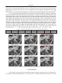
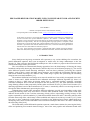
PDE-BASED RESTORATION MODEL USING NONLINEAR SECOND AND FOURTH
ORDER DIFFUSIONS
Tudor BARBU*
*
Institute of Computer Science of the Romanian Academy
Corresponding author: Tudor BARBU, E-mail: [email protected]
In this article we propose a novel image denoising and restoration system based on a combination of
second and fourth order partial differential equations. We consider a variational scheme that
minimizes a energy functional composed of functions of gradient magnitude and of absolute value of
Laplacian of image intensity. Then the corresponding Euler-Lagrange equation is computed, a PDE
model based on second and fourth order nonlinear diffusions being achieved. A robust mathematical
treatment is provided for this nonlinear diffusion model. Then, a consistent numerical approximation
scheme based on a finite-difference method is proposed.
Key words: image denoising and restoration, variational PDE model, nonlinear anisotropic diffusion,
fourth order PDE, Euler-Lagrange equation, mathematical treatment, numerical discretization scheme
1. INTRODUCTION
Since detail-preserving image restoration still represents a very serious challenge for researchers, the
partial differential equations have been investigated as useful tools for image enhancement in the last
decades [1]. That is because the PDE-based techniques are able to achieve a proper trade-off between noise
reduction and image feature preservation.
The conventional two-dimensional filtering approaches have the disadvantage of blurring the image
boundaries and possibly destroying other details, and also they have no localization property [2]. The second
order diffusion equation based denoising techniques overcome these problems, preserving the essential
features, such as edges, corners and other sharp structures, and avoiding the localization problem. These
PDE-based methods encourage the diffusion only within image regions, thus performing the smoothing
along but not across the boundaries [1,3].
The nonlinear diffusion-based image noise removal models have been widely investigated since 1987,
when P. Perona and J. Malik introduced their influential anisotropic diffusion algorithm [4]. Since it is
common to derive a PDE image processing model from a variational problem, numerous variational
restoration techniques have been also developed in the last decades [3,5]. The most influential variational
image filtering scheme is that proposed by Rudin, Osher and Fetami in 1992 [6]. Their Total Variation (TV)
denoising algorithm, based on the minimization of TV norm, is remarkably effective at removing the noise in
flat regions while simultaneously preserving the edges.
Although these second order anisotropic diffusion techniques provide good smoothing results while
avoiding the blurring effect, they often fail to overcome other undesired effects. Thus, most second order
diffusion based models do not avoid the staircasing (blocky) effect, representing creating in image of flat
regions separated by artifact boundaries [5]. Both Perona-Malik framework and TV denoising scheme suffer
from this staircasing effect, which many of their modified and improved versions try to reduce [3,5,7]. In the
last years we have conducted a high amount of research in the diffusion-based image enhancement area,
developing some robust second order PDE based restoration techniques that remove or reduce considerably
the staircasing effect [8-10].
The fourth-order partial differential equations represent a much better solution for removing the blocky
effect and producing more natural denoised images. One of the most popular and influential fourth order
PDE-based restoration model using second and fourth order diffusions
2
PDE based smoothing model was introduced by Y. L. You and M. Kaveh in 2000 [11]. Their algorithm
approximates the observed image with a piecewise harmonic one. Another influential denoising scheme
based on fourth order PDEs was proposed in 2003 by M. Lasaker, A. Lundervold and X. Tai [12]. We also
proposed a fourth-order PDE-based restoration method derived from You-Kaveh scheme, which was
successfully applied for noisy sonar images and video sequences [13].
While these fourth order diffusion models achieve satisfactory denoising results, alleviating the
staircasing effect and providing more natural images, they perform somewhat poorer on preserving the
boundaries and textures. Also, they are outperformed at removing the speckle noise by the second-order
anisotropic diffusion-based techniques. In order to improve the classic fourth-order PDE models, numerous
modified and combined denoising approaches have been introduced. Some of them use combinations of
second-order and fourth-order diffusions to obtain better smoothing results [14].
We propose a novel combined PDE-based model, containing both second order and fourth order
diffusion components, in this paper. Our nonlinear anisotropic diffusion technique achieves very good edgepreserving image restoration results, while removing successfully the staircasing effect and also the speckle
noise. The developed denoising framework is described as both a variational (minimization) problem and a
diffusion model in the next section. A rigorous mathematical investigation of this PDE scheme is performed
in the third section, where we analyze the existence, uniqueness and character of its solution. In the fourth
section we provide a numerical discretization scheme for the proposed model. The performed experiments
and method comparison are described in the fifth section. The article finalizes with a conclusions section, the
acknowledgements and a list of references.
2. NONLINEAR DIFFUSION EQUATION-BASED IMAGE RESTORATION MODEL
In this section we consider a novel PDE-based image denoising and restoration solution that is intended
to optimize the trade-off between smoothing, feature preservation and staircasing removing [1]. Thus, we
consider a variational model [15] that minimizes an energy cost functional based on functions of the image
intensity Laplacian and of the gradient magnitude. Therefore, the restored image will be determined as:
u *  arg min J ( u )
(1)
u
where
J (u ) 
  u 
1


2
2
u


2

u
 u0

2
(2)
d
where  1 and  2 represent two regularizer functions,    0 ,1  and u 0 is the observed image. The first
smoothing term of the energy functional J assures that the denoising process is performed along the gradient
direction, while the second one uses the Laplacian to approximate the observed image with a planar one,
since the Laplacian value at a pixel becomes zero if its neighborhood is planar [2]. The third component is
introduced to encourage the similarity to the original image.
A robust nonlinear diffusion model is derived from this variational PDE scheme, by computing the
corresponding Euler-Lagrange equation [15]. Thus, from (1) and (2) one obtains the following EulerLagrange equation:

where 
u
1
,
u
2
: 0 , 
2
  
u
2
2



u  u  div 
2
   0 ,   , with  1u ( s ) 
u
1
  u  u  
1  1 (s)
s
s
and 
u
2
 u  u 0
(s) 
by applying the gradient descent, one obtains the following PDE model:

1  2 (s)
s
s
(3)
respectively. Then,
3
Tudor Barbu
 u

 div 
 t



u
1
  u  u  

2
  
u
2
2


u  u   u  u 0
2

(4)
u 0 , x , y   u 0
where u 0 represents the initial noisy (degraded) image. The PDE given by (4) constitutes a nonlinear
diffusion model whose positive and monotonic decreasing diffusivity functions are selected as follows:











u
1
u
2


2

 
s 
(s)   
  k ( u ) log


  k (u ) 

1 ,
 (u )
(s)  
s  
, s  0
10

s 




 k (u ) 
(5)
for s  0
, s  0
where  ,  ,   1,8  ,  ,    0,1  and parameters k and  are modeled as functions of the current
state of evolving image, u. They are based on some statistics of gradient and Laplacian of intensity function:

 k (u )       u

 ( u )  median




r  ord ( u )
2
u
(6)
 4
where    2,3  , r   0,1  ,  represents the averaging operator, ord (u) returns the order of u in the
evolving image sequence, while median computes the current image’s median value. The denoised image
will be obtained as a solution of this PDE restoration model. So, existence and uniqueness of such a solution
is demonstrated in the next section, where a mathematical treatment of our diffusion scheme is performed.
3. MATHEMATICAL INVESTIGATION OF THE PDE-BASED DENOISING SCHEME
A rigorous mathematical treatment of the PDE restoration model proposed in previous section has to
be performed now. First, one could demonstrate easily that the diffusivity functions of the PDE given by (4)
have been properly selected [10]. From (5) - (6) it results that 
s  0
.
Also,
both
of
these

 s1


 k (u )

u
1




 k ( u ) log
u
1
10
 s1


 k (u )
( s 2 ),  s 1  s 2 ,




and 
monotonically
 s2


 k (u )
and also 
u
2




2
 k ( u ) log
( s1 )   
We have also lim  1u ( s )  lim  2u ( s )  0 and 
s 
are
(s)  0
s 
u
1
10

  s1  
(0 )  1
 s2


 k (u )
  
u
2




 (u )
(s)  
decreasing.


2
( s1 )  
functions
u
1
,  s1  s 2

  s2  
s  
 0
,
Since
we
have
it
results
that
,

u
2
( s 2 ),  s 1  s 2
.
, therefore the diffusivity functions are properly
selected for a successful diffusion [10]. Now, an analysis of the existence of the solution of equation (4)
should be performed. So, our modeled PDE has solution if the functions s   1u ( s ) and s   2u ( s ) are
monotonically increasing. In order for this to happen, their derivatives have to be positive. Since

s
s 
u
i

(s)  
u
i
(s)  s

u
i
s
(s)
, i  1 , 2  ,
it results that the next conditions must be satisfied:
PDE-based restoration model using second and fourth order diffusions








u
1
u
2
s  
s
s  
s

s

u
2
u
1
s  
s

u
1
s 
s
2
 k (u )

s
ln 
 k (u )
, this leads to 
u
1
s  
s

u
1

k (u ) 
s
 k (u )  
 1  ln 
 

2
 ln( 10 )
s
k (u )




2
2



s
k (u )
s



ln 

 k (u ) 2
ln( 10 )
 k (u ) 


u
1
s  
s

u
1
s
s 
s 
s

condition according to (7). If
 0
,s  0
, that is true, for s = 0. If s > 0, we get



k ( u ) ln 
 2s

 

2
k (u )

s

s ln 

 k (u )

 s










k ( u ) ln
2


s
 
 

k (u ) 
ln(



s
2

 k (u ) 2






 0

 
s

 
 k (u )  

10 )



2
. If


s
2s
k (u )
 
ln 

2

ln( 10 )
ln( 10 )
k (u )
 k (u ) 
2
k (u )




2
, for k ( u )  ln( 10 ) that is a generally verified
, the first condition of (7) is usually not satisfied, because
2
 k (u ) 



s
s
 ln 
 


1
2



 ln( 10 ) 
k (u )
 k (u ) 










 ln( 10 ) 






k (u ) 
s
2



s
k (u )
s



ln 

 k (u ) 2
ln( 10 )
 k (u )  

2
s  k (u )

(7)
 0
ln( 10 )


1  0




s




 k (u ) 
s  k (u )
s 
s
The first condition is equivalent to  1u  0  

s 
u
1
4



s
k (u )
s

 

ln 
 k (u ) 2

ln( 10 )
 k (u )  

2
2




 0
, for
k (u )
given by (6) and s also
related to the magnitude of the intensity gradient. The second condition of (7) is always satisfied because
u
  2 s 
 (u )
   (u )
u
 2 s   s
 
 s
 0,  s  0.
s
s  
 s
 

2
 (u )
s  
Although the first condition is not verified for s  k (u ) , our PDE problem is well-posed, so its
solution exists and is also unique, because we get s  k (u ) for the vast majority of the pixels of u, as it
results from (6). The much fewer pixels corresponding to s  k (u ) are related to noise or some very sharp
edges encountered, their number decreasing as u is evolving, while the most pixels correspond to s  k (u ) ,
being located within the more homogeneous regions of u.
Given the conditions of (7), the proposed nonlinear diffusion model represents a forward parabolic
equation, therefore it has a weak unique solution, it is a stable PDE and its finite difference based numerical
approximation scheme has consistency property. The stability property means that its solution converges to
5
Tudor Barbu
lim u ( t , x , y )  u
the solution of the variational problem formulated in (1) - (2). So,
*
t 
, where
u
*
is given by
(1). This solution is numerically computed by the PDE discretization scheme proposed in the next section.
4. A CONSISTENT NUMERICAL APPROXIMATION ALGORITHM
A discretization solution to the developed continuous PDE model is described in this section. So,
according to the mathematical treatment provided in previous section, a consistent numerical approximation
using finite differences can be modeled for our nonlinear diffusion model [16]. We perform the PDE
discretization by considering a space grid size of h and a time step  t , respectively. The space and time
coordinates are quantized as following:
x  ih , y  jh , t  n  t ,  i  0 ,1 ,..., I , j  0 ,1 ,..., J , n  0 ,1,..., N

(8)
The PDE model given by (4) is approximated through a finite-difference technique [16]. The second
part of the model is computed much easier, being related to Laplacian operator that is discretized as follows:
u (i  h , j )  u (i  h , j )  u (i, j  h )  u (i, j  h )  4 u (i, j )
n
 u (i, j )   u (i, j ) 
2
n
n
n
n
n
h
n
2
(9)
where the boundary conditions are the following:
u (  1 , j )  u ( 0 , j ), u ( I  1 , j )  u ( I , j ), u ( i ,  1 )  u ( i , 0 ), u ( i , J  1 )  u ( i , J )
n
n
n
n
n
n
n
n
(10)
Then, by using (9), one computes the following functions:
f 1 (i, j )  
n
u
2

2
n
u
i , j   2 u n i , j 
(11)
and next applies the discrete Laplacian operator on them, obtaining the following result:

2
  
u
2
2
u
n
 i , j   2 u n  i , j   
f
n
(i  h , j )  f
n
(i  h , j )  f
n
(i, j  h )  f
h
n
(i, j  h )  4 f
n
(i, j )
(12)
2
with some boundary conditions similar to those formulated in (10). The numerical approximation of the first
component of our diffusion model requires more computations. Therefore, we have:

div 
u
1
  u  u      u  u
u
1

  
u
1
  u    u
(13)
where the first part of this sum is approximated, by using the discretized Laplacian given in (9), as
f 2 (i, j )  
n
u
1
 u
n

(i, j )  u (i, j )
2
n
(14)
while the second part is computed as follows:
 
u
1

that leads to

 
 u    u  

 x

u
1





 u 


 x 
2
 u
 
 y




2

 
,

 y


u
1





 u 


 x 
2
 u
 
 y




2





 u u
 
,
 x y




(15)
PDE-based restoration model using second and fourth order diffusions

 
u
1
  u    u



u
1
s

u
1
s

6

2
2
2
2
 u  u
u  u
u  u
u  u



2
2
x xy
x x
y xy y y
 u 
,
2
2
2
2

 u 
 u 
 u 
 u 




  

  



 x 
 x 
 y 
 y 

 u 
 u 


 x 
2
 u
2
x
 u 

 

x y xy
 y 
u u  u
2

2
 u 


 x 
2
2
 u 

 

 y 
 u








2
y
 u u
 
,
 x y




(16)
u u  u
2

2
x y xy
2
Then, we perform some approximations in the above formula to simplify the computation. So, since
we have observed that the second order derivatives do not vary so much, (16) is transformed as following:
 u  u
u



xy  x
y
2

 
u
1
  u    u
so, we compute


u
 u 
1
s
f 3 (i, j ) 
n
 u 


 x 

u
1
s





2
 u 

 

 y 
  u (i, j ) 




x


n




2
2







u
1
s
2
  u (i, j ) 

 


y


n
2
 u 


 x 
2
 u
 
 y




2

2
  u
 xy


 u
u



y
 x
 2 n
n
n
 u (i, j ) 
  u (i, j )   u (i, j )






xy
x
y





 u (i, j )
 u (i, j )
u (i  h , j )  u (i  h , j )  u (i, j  h )  u (i, j  h )




x
y
2h
 2 n
n
n
n
n
 u (i, j )
u (i  h , j  h )  u (i  h , j  h )  u (i  h , j  h )  u (i  h , j  h )


2

xy
4h

n

n
and   1u  s    u ( i , j )



n


x 
2
n
n
2 
n
  u (i, j )
 
 

y  


n




(17)
, where
n
(18)
is computed as in section 3, using (5). So, by combining all these
discretization results, we get the numerical approximation scheme corresponding to the PDE modeled by (4):
u
n 1

(i, j )  u (i, j )   t f 2 (i, j )  f 3 (i, j )  
n
n
n
2



f 1 ( i , j )   u ( i , j )  u ( i , j ) , i  0 ,.., I , j  0 ,.., J  (19)
n
n
0
where u 0 represents the discrete form of the initial image. Our iterative denoising algorithm starts with this
initial  I  J  image and applies repeatedly the process given by (19), on the evolving image u n , for each n
from 0 to N. Its third term prevents the image degradation after reaching the optimal denoised form. The
developed numerical scheme is consistent with the PDE model, and also stabile and convergent [16]. It
converges fast, in a low number of steps N, to the solution of our PDE, which is the restored image u N  1 .
5. EXPERIMENTS
The proposed nonlinear diffusion-based restoration scheme was tested on hundreds of images
corrupted with various levels of Gaussian noise. It has a low execution time, of approximately 1s, and a high
7
Tudor Barbu
effectiveness: removing a high amount of noise, while preserving well the image edges and reducing the
staircasing. The optimal noise removal results were obtained for some properly selected parameters of the
PDE model:   1 . 5 ,   0 .7,   8,   4,   0.04,   2.4, r  0 .03 ,  t  0 . 25 , h  1, N  25. The
performance of our image denoising technique was measured using the Peak Signal-to-Noise Ratio (PSNR).
We also performed method comparison and found that our nonlinear diffusion technique outperforms
both the conventional and PDE-based restoration approaches. It produces much better denoising results than
conventional filters, such as 2D Gaussian, average, Wiener or median [2], unlike them, overcoming the
blurring effect and preserving the image details [1]. Our restoration PDE model also provides a better noise
removal than some influential or state of the art diffusion-based schemes. Thus, it outperforms the secondorder diffusion-based methods, like both versions of the Perona-Malik framework [4] and TV denoising [6],
achieving a better restoration, converging faster and avoiding the staircasing effect. Also, the proposed
anisotropic diffusion technique performs better than fourth-order isotropic diffusion models, like You-Kaveh
scheme [11], achieving superior edge preservation and converging to optimal solution in fewer iterations.
One can see in Table 1 that our method gets higher PSNR values than Perona-Malik, TV, You-Kaveh, [3x3]
2D Gaussian and Median image filters. It is also obvious from Fig. 1 (c) that our system provides the best
denoising for the 51 2  512  Barbara image affected by Gaussian noise (avg. = 0.21 and var = 0.02).
Table 1. Comparison of the PSNR values for several image de noising techniques
Method
PSNR
Barbu model
28.34(dB)
P-M 1
26.23(dB)
P-M 2
24.91(dB)
TV
21.88(dB)
You-Kaveh
27.19(dB)
Gaussian
21.37(dB)
Median
24.53(dB)
Fig.1. Barbara image restored by various filters (see the red-marked denoising result of our PDE model)
6. CONCLUSIONS
In this article we proposed a novel PDE-based image restoration system based on a combination of
second-order and fourth-order diffusions. It is derived from a variational model and is intended to overcome
PDE-based restoration model using second and fourth order diffusions
8
the undesired effects that affect the second order or fourth order PDE based denoising techniques. Our
nonlinear diffusion-based approach performs an effective feature-preserving image smoothing, while
reducing considerably the blurring effect that affects the conventional filtering [2] and somewhat the fourthorder PDE-based restoration [11-13], the blocky effect that alters the second-order PDE-based denoising [4],
and the speckle noise that is not fully removed by the fourth order PDE models [11,12]. Thus, the combined
technique proposed here represents a better denoising solution than well-known classic filters [2], secondorder diffusion methods, such as Perona-Malik schemes [4], Total Variation [6], and even their improved
versions [5,7], and fourth-order PDE models, such as You-Kaveh isotropic diffusion and its derived methods
[11,13]. Also, our diffusion model has an anisotropic character, converges fast and has a low execution time.
The considered variational problem, the derived PDE model composed of second and fourth order
diffusion components, and the proposed numerical approximation scheme represent the main contributions
of this paper. Also, we provided a robust mathematical analysis of the proposed model, investigating
rigorously the well-posedness of our problem. Our successfully experiments provided satisfactory restoration
results that can be further used in other image analysis and computer vision domains [2,3,5], such as
boundary and image object detection, which will be approached as part of our future research.
ACKNOWLEDGEMENTS
The author acknowledges the valuable research support of the German Academic Exchange Service
(DAAD), this research being conducted as part of his DAAD project VANDIRES, Code No. A/14/02332. He
also acknowledges the support of Institute of Computer Science of the Romanian Academy, Iași, Romania.
REFERENCES
1.
2.
3.
4.
5.
6.
7.
8.
9.
10.
11.
12.
13.
14.
15.
16.
H. E. NING, L. U. A. KE, A Non Local Feature-Preserving Strategy for Image Denoising, Chinese Journal of Electronics, vol.
21, no. 4, 2012.
R. GONZALES, R. WOODS, Digital Image Processing, 2nd ed., New York: Prentice Hall, 2001.
F. GUICHARD, L. MOISAN, J. M. MOREL, A review of P.D.E. models in image processing and image analysis, Journal de
Physique vol. 4, pp. 137–154, 2001.
P. PERONA, J. MALIK, Scale-space and edge detection using anisotropic diffusion, Proc. of IEEE Computer Society Workshop
on Computer Vision , pp. 16–22, 1987.
J. WEICKERT, Anisotropic Diffusion in Image Processing, European Consortium for Mathematics in Industry, B. G. Teubner,
Stuttgart, Germany, 1998.
L. RUDIN, S. OSHER, E. FATEMI, Nonlinear total variation based noise removal algorithms, Physica D: Nonlinear
Phenomena, 60, 1, pp. 259-268, 1992.
B. WAHLBERG, S. BOYD, M. ANNERGREN, Y. WANG, An ADMM algorithm for a class of total variation regularized
estimation problems, in Proc. of 16th IFAC Symp. Syst. Identificat., pp. 1–6, July 2012.
T. BARBU, Variational Image Denoising Approach with Diffusion Porous Media Flow, Abstract and Applied Analysis, Volume
2013, Article ID 856876, 8 pages, Hindawi Publishing Corporation, 2013.
T. BARBU, A Novel Variational PDE Technique for Image Denoising, Lecture Notes in Computer Science (Proc. of the 20th
International Conference on Neural Information Processing, ICONIP 2013, part III, Daegu, Korea, Nov. 3-7, 2013), Vol.
8228, pp. 501 - 508, Springer-Verlag Berlin Heidelberg, M. Lee et al. (Eds.), 2013.
T. BARBU, A. FAVINI, Rigorous mathematical investigation of a nonlinear anisotropic diffusion-based image restoration
model, Electronic Journal of Differential Equations, Vol. 2014, No. 129, pp. 1-9, 2014.
Y. L. YOU, M. KAVEH, Fourth-order partial differential equations for noise removal, IEEE Transactions on Image Processing,
9, pp. 1723–1730, 2000.
M. LYSAKER, A. LUNDERVOLD, X. C. TAI, Noise removal using fourth-order partial differential equation with applications
to medical magnetic resonance images in space and time, IEEE Transactions on Image Processing, vol.12, no.12, pp.
1579-1590, 2003.
T. BARBU, A PDE based Model for Sonar Image and Video Denoising, Analele Științifice ale Universității Ovidius, Constanța,
Seria Matematică, Vol. 19, Fasc. 3, pp. 51-58, 2011.
H. WANG, Y. WANG, W. REN, Image Denoising Using Anisotropic Second and Fourth Order Diffusions Based on Gradient
Vector Convolution, Computer Science and Information Systems, Vol. 9, pp. 1493-1512, Dec. 2012.
M. HAZEWINKEL, Variational calculus, Encyclopedia of Mathematics, Springer, ISBN: 978-1-55608-010-4, 2001.
P. JOHNSON, Finite Difference for PDEs, School of Mathematics, University of Manchester, Semester I, 2008.
Received September 8, 2014