1
EDACC
User Guide
version 0.1
c
Copyrightby
Adrian Balint, Daniel Diepold, Daniel Gall, Simon
Gerber, Gregor Kapler, Robert Retz, Melanie Handel
Abstract
We present the main capabilities of EDACC and describe how
to use EDACC for managing solvers and instances, create experiments with them, launch them on different computer clusters,
monitor them and then analyze the results.
Contents
1 Outline
3
2 Introduction
3
2.1
General Terms . . . . . . . . . . . . . . . . . . . . . . . .
3
2.2
Motivation
. . . . . . . . . . . . . . . . . . . . . . . . . .
3
2.3
EDACC Components . . . . . . . . . . . . . . . . . . . . .
4
2.4
System Requirements
. . . . . . . . . . . . . . . . . . . .
5
2.5
Getting started . . . . . . . . . . . . . . . . . . . . . . . .
5
3 Graphical User Interface
6
3.1
Database connection . . . . . . . . . . . . . . . . . . . . .
6
3.2
Modes . . . . . . . . . . . . . . . . . . . . . . . . . . . . .
7
3.3
Manage DB Mode . . . . . . . . . . . . . . . . . . . . . .
8
3.4
Experiment Mode
. . . . . . . . . . . . . . . . . . . . . .
12
3.5
Property . . . . . . . . . . . . . . . . . . . . . . . . . . . .
17
4 Parameter search space specification
4.1
Example . . . . . . . . . . . . . . . . . . . . . . . . . . . .
20
22
5 Client
23
5.1
Introduction . . . . . . . . . . . . . . . . . . . . . . . . . .
23
5.2
System requirements . . . . . . . . . . . . . . . . . . . . .
23
5.3
Usage . . . . . . . . . . . . . . . . . . . . . . . . . . . . .
24
5.4
Verifiers . . . . . . . . . . . . . . . . . . . . . . . . . . . .
26
5.5
Experiment priorization . . . . . . . . . . . . . . . . . . .
26
6 Web Frontend
2
28
6.1
Introduction . . . . . . . . . . . . . . . . . . . . . . . . . .
28
6.2
System requirements . . . . . . . . . . . . . . . . . . . . .
28
6.3
Installation . . . . . . . . . . . . . . . . . . . . . . . . . .
28
6.4
Configuration . . . . . . . . . . . . . . . . . . . . . . . . .
30
6.5
Troubleshooting . . . . . . . . . . . . . . . . . . . . . . . .
30
6.6
Features . . . . . . . . . . . . . . . . . . . . . . . . . . . .
30
6.7
Result pages . . . . . . . . . . . . . . . . . . . . . . . . . .
32
6.8
Analysis pages . . . . . . . . . . . . . . . . . . . . . . . .
33
7 Automatic Algorithm Configuration
35
8 Monitor
35
9 Troubleshooting
35
10 Glossar
36
EDACC User Guide
1
Outline
Here we will have an overview of this user guide specifying where the user
can find what!
2
2.1
Introduction
General Terms
To keep this user-guide consistent we would like to define a couple of
terms that will be often used through this document. Even if you are
familiar with these, we recommend you to take a short look at them.
Algorithm
Example 1:
We define an algorithm as an arbitrary computation method.Examples
of well known algorithms are the family of sorting algorithms like bubblesort, quick-sort or merge-sort.
Solver
The concrete implementation of an algorithm in an arbitrary programming language is called a solver, which normally has an input and an
output.
Instance
A solver is designed to solve a certain type of problem.One concrete
problem (an instantiation of it) is called a (problem) instance . For the
sorting algorithms an example of an instance would be a file containing
a sequence of number that has to be sorted.
Example 2:
Solver Parameters
To control the behavior of a solver it can have parameters which we
will call solver parameters. These parameters can also be seen as an
input of the solver which is normally passed through the command line.
For example the quick-sort algorithm could have a parameter “pivot”
that can take the values {lef t, right, random}. With the help of this
parameter the behavior of the solver can be controlled regarding how it
should choose the pivot element during sorting.
Solver Configuration
A solver together with a fixed set of values for its parameters is called a
solver configuration. Randomized quick-sort would be a solver configuration of the quick-sort solver with the parameter “pivot” set to random.
Computing System
To see how a solver performs on a certain instance we need to execute that
solver. For this task we need a computing system which in EDACC
ca be a single computer, computer cluster of even a grid.
Instance Property
Result Property
2.2
As EDACC provides a wide variety of statistical analysis tools we need a
way to point out different forms of informations. We define an instance
property as any kind of information that can be extracted from an
instance. The output of a solver is called the result and any information
that can be computed from the result is called result property.
Motivation
Algorithm engineering:
EDACC User Guide
When designing and implementing algorithms one is at the end of the
process confronted with the problem of evaluating the implementation on
the targeted problem set. As the authors of EDACC are familiar with
algorithms for the satisfiability problem (SAT) we will take this sort of
algorithms as further examples. After designing and implementing a SAT
solver we would like to see how it performs on a set of instances (let us
suppose that our solver is an implementation of a stochastic one i. e.,the
result of the solver on the same instance will be a random variable).
3
Normally we would start our solver on each instance and record the runtime or some quality measure. This is a sequential process and could
be easily performed with the help of simple shell script. But there are
some questions that have to be answered before starting the evaluation
process.
1. How long is the solver allowed to compute on one instance? And
how do we restrict that?
2. In the case of randomized solvers, how often do we call the solver
on each problem set?
3. Do we limit the resources used by the solver (i. e.,maximum of memory, maximum stack size)?
Example 3:
Let us now suppose we would like to test our SAT-solver on 100 instances
where we allow a timeout of 200 seconds. Because of the stochastic nature
of the solver we are going to run it for 100 times on each instances. We
are not going to limit other resources. Now we get a set of (100 instances)
× (100 runs) that produces a set of 10000 jobs. Having a timeout limit of
200 seconds our computation could take up to 10000·200 = 2000000sec ∼
=
24days on a single CPU machine in worst case.
Now everybody has access to multi-core machines or even some clusters
with multiple CPU’s. So we could speed up the computation by using
this sort of resources but then we get the problem of equally spreading
our jobs. And more than that we have to collect the results after that
and process them with some statistical tools.
Most of the researchers solve this problems by writing a collection of
scripts. This solution is error-prone and time consuming because there
is no very simple way to equally spread jobs across multiple machines.
Collecting the results and merging them together can also yield a not
negligible amount of work. One more disadvantage is that the results
can be seldom reproduced without having the complete set of scripts and
even then there might be some steps that are not incorporated within
the scripts.
EDACC features
To solve this problems we have designed EDACC. The main goal of
EDACC are to:
1. manage solvers and instances and archiving them in a database
with the help of a GUI
2. create experiment settings by configuring solvers and selecting the
instances
3. evaluating the jobs of an experiment on arbitrary many machines
4. provide analysis tools for the results
5. provide an online tool to monitor and analyze experiments
2.3
EDACC Components
The four major components of EDACC are the:
1. Grapical user interface (GUI)
2. Database (DB)
3. Compute client (client)
4. Web frontend (WF) (optional)
4
EDACC User Guide
2.4
System Requirements
! →
1. GUI - Sun Java 6 (JRE 6), optional: R (see Experiment Mode README.txt for more details)
! →
2. Database - MySQL version 5.1 or above, tested with version 5.1.41
on Ubuntu. The machine the database runs on is the most important factor of the performance of EDACC. The following components will have the greatest impact on database performance:
• The more RAM MySQL can use, the less it has to access slow
hard disks on read-transactions. It also enables MySQL to
keep indexes and whole tables in memory. This will greatly
affect the ability to work on multiple experiments at the same
time.
• Hard disk performance is not as important as RAM but all
data has to be written to the disk eventually which is when
fast access time and write throughput become important.
• A fast multi-core CPU will enable MySQL to handle more
requests concurrently but is not as important as RAM.
Network latency and bandwidth should also be considered when
the GUI and clients are run on remote machines. The clients will
write the output of solvers and metadata back to the database so
the required bandwidth depends on the size of the generated output
and metadata.
2.5
! →
3. Client - see section 5.2
! →
4. Web Frontend - see section 6.2
Getting started
To use EDACC you will have to follow these steps:
1. Set up a mysql database (see 2.5.1.
2. Download the latest EDACC GUI from sourceforge.org (eventually
check for updates within EDACC).
2.5.1
MySQL Installation and Setup
MySQL configuration
MySQL installation is simple on most Linux distributions. On Ubuntu,
for example, you have to type apt-get install mysql-server and set a
root account password when the installation procedure asks you to. After
installation there are a few settings that have to be adjusted in order to
use MySQL with EDACC. These can be found in the configuration
file my.cnf usually located at /etc/mysql/my.cnf. Adjust the following
settings:
[mysqld] # look for this section
# listen on all IPs/allow network connections :
bind-address = 0.0.0.0
# maximum packet size (important for large instances):
max_allowed_packet = 2048M
# enable event scheduler
event_scheduler = 1
EDACC User Guide
5
# comment out the skip-networking directive,
# if present:
#skip-networking
# increase session timeout
# and maximum number of simultaneous connections
wait_timeout = 259200
max_connections = 1000
# performance related settings
# innodb_buffer_pool_size is the most important parameter
# set this to as much RAM as you can spare on the machine:
innodb_buffer_pool_size = 1024M
Creating databases
After saving the modifications, restart your MySQL server (Ubuntu:
service mysql restart) and open a MySQL client session by typing
mysql -uroot -p which will then ask you for the root password you
specified during MySQL installation. In the MySQL client shell you can
then create an empty database that can be used as EDACC database
by running the following commands:
CREATE DATABASE edacc;
GRANT ALL PRIVILEGES ON edacc.* TO ’edaccuser’@’%’
IDENTIFIED BY ’dbuserpassword’ WITH GRANT OPTION;
This will create an empty database called edacc and grant the MySQL
user edaccuser with the password dbuserpassword all necessary rights.
In the EDACC GUI, client and Web Frontend you can then use this
account when connecting to the database.
2.5.2
Starting the GUI
If you have succeeded to set up a database now you can start the GUI of
EDACC by typing:
java -jar EDACC.jar
3
3.1
Graphical User Interface
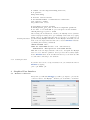
Database connection
Every time you will start EDACC you will be prompted to provide the
TM
connection data to the MySQL database you would like to work with.
6
EDACC User Guide
Host name / IP
In the connection dialog you have to provide the host name or the IPTM
address of your MySQL database.
Port
If you have configured the MySQL server to use an other port then the
TM
default MySQL port 3306, you can specify this in the Port: text field.
DB name
Further you also have to provide a valid database name and a user along
with the corresponding password.
Save password
If you would like to save the password of this connections for further
usage you can check the Save password check-box. EDACC will save
the password for you in a configuration file. The password is saved in
plain text, so if other users have access to your private files they will be
able to read the password from the configurtion file.
! →
Max Connections
EDACC is a multi-threaded program and will use more than on connection to the database to speed up certain tasks. We recommend to allow
up to 8 simultaneous database connections, but if you have restrictions
on this number you can specify it in the Max Connection: text field.
SSL connections
If you are going to use EDACC to store trusted data we strongly recommend to enable a SSL connection by checking the secured connection
check box. Be aware that this kind of connection is only possible is the
TM
MySQL server is configured accordingly.
Compressed Connections
When working with EDACC through a slow network connection you
might want to turn on compression by checking the compress connection check box.
Connect
3.2
TM
After providing all the information you can connect to the MySQL
TM
server.
Create DB
When you connect the first time to a database EDACC will create for
you all the needed tables.
DB Model version
As EDACC is under full development and the database model may be
extended to support new features, EDACC will check if the database
model is compatible with the GUI version. Within this check we differentiate between two cases:
DB Model upgrade
1. The database model version is to old for the GUI. In this case
EDACC will offer you the possibility to upgrade your database
scheme to the latest version.
GUI update
2. The database model version is to new for the GUI. In this case
you should update the GUI. You can do this by using the automatic update function of EDACC, which can be found under Help
→ Check for Updates. Another possibility is to download the
latest release form the project site at http://sourceforge.net/
projects/edacc/.
Modes
EDACC is split up in two modes:
1. Manage DB Mode
2. Experiment Mode
There is a strict split-up between these two modes. You can be only in
one mode when working with EDACC. When starting EDACC you will
always be in the the manage DB mode, which will allow you to manage
your solvers and instances before creating experiments with them. To
EDACC User Guide
7
switch between modes you have to choose the desired mode from the
menu bar Mode.
3.3
Manage DB Mode
The manage DB Mode is again split up in several parts: solvers, instances,
verifiers and result codes. Those parts can be reached by clicking on the
corresponding tab.
3.3.1
Solvers
Solver
Solver name
Solver version
Solver description
Solver authors
Solver code
As mentioned in section 2.1 a solver is a program which implements
an algorithm. In EDACC we store the following information about a
solver:
1. A human-readable name of the solver.
2. The version number of the solver. The combination of name and
version must be unique.
3. A short description of the solver.
4. The list of the authors of a solver.
5. The sourcecode of the solver.
Solver binaries
6. A solver can consist of different binaries, which have the same
source code but differ in the compile options (eg. the architecture)
or the chosen compiler version. There must be at least one solver
binary.
Parameters
Every solver has a list of several parameters which control its behaviour.
To build a valid parameter list string, EDACC needs the following information:
name The human-readable internal name of the parameter. This name
has no effect to the generated command-line and is only needed for
reasons of indentification in the EDACC system.
prefix The parameter prefix defines how the parameter is called on the
command-line. The Unix program ls for example has a parameter
with the prefix -l.
Boolean Some parameters don’t have an actual value but act as switches for
a certain functionality of a solver. The -l parameter of the Unix
program ls for example is such a boolean parameter.
Mandatory Some parameters need to be specified to start the solver binary.
Such parameters are called mandatory.
Space Specifies if there has to be a space between parameter prefix and
value.
Order Some solvers need a special order of the parameters. This order is
specified by an ascending number. The parameter with the smallest number will be used first in the command-line string. If two
parameters have the same order number, the order between those
two parameters doesn’t matter.
Add Solver
8
By clicking the button “New” in the solver panel, a new empty line in the
solver table is created. To fill the new entry with information fill in the
form below the table with the static information of the solver. Optionally
EDACC User Guide
you can attach the code of the solver to the entry by clicking on “Add
Code” and choosing the files or directories from your file system.
! → To create a valid solver entry, it is necessary to specify at least one solver
binary.
Add Solver Binary
The table below the text fields with the static solver information shows
the solver binaries which are already attached to the chosen solver. To
add another binary, click on the “Add” button below the table with the
binaries. Choose the binary files which are needed to run the solver from
your file system. EDACC then tries to zip the chosen files. This can take
a few seconds.
To complete the process, some information on the binary have to be
given:
Alternative Binary Name A human-readable name of the binary. This information is only
needed that the binary can be recognized by the user in the program.
Execution File The main file of the binary, which will be called by the EDACC
client to start the binary. You can choose it from the list of the
previously chosen binary files. For default, the first file is chosen.
Additional run command Some binaries or scripts need a special command to start them (this
is very usual for interpreted languages or scripts). For example a
Java JAR archive can be started by the additional run command
java -jar. A preview of the command executed on the grid by the
client is shown in the text line below the text field for the addtional
run command.
Version The version string specifies for example the architecture of the compiled binary or the used compiler. The version of the underlying
source code is specified in the solver information, which is described
above!
Click on “Add binary” to complete the process.
! → All modifications on solvers, solver binaries or parameters are not directly
saved to the database. To persist your changes, you can choose the button
“Save To DB”.
Edit Solver
To edit the information of a certain solver, choose the solver from the
solver table. The text fields below the table will show the currently saved
information of the solver. By changing those values, the information in
the solver table will be adjusted automatically.
Edit Solver Binary
There are two ways to edit a solver binary: First, by clicking on “Edit”
below the solver binary table, the user can update the information of
the selected binary like its name, its execution file or the additional run
command without changing the files of the binary.
Additionally, it is possible to select a bunch of new files to be assigned
to a binary. The existing files will be lost in this case! After choosing
new files, the solver binary information dialogue will be shown, where the
information of the binary can be changed.
Delete Solver Binary
To delete a solver binary, choose it in the list of binaries and click on the
! → “Delete”-Button below the table. After confirming the delete action, the
solver binary will be removed directly from the database!
Delete Solver
EDACC User Guide
If you want to delete a solver with all attached information, code, binaries
and parameters, click on the “Delete”-Button in the solver panel. The
9
solver will be removed directly from the database, after confirming the
delete action. To delete multiple solvers at once, just hold Ctrl in the
solver table.
Add Parameter
! →
Edit Parameter
If you want to edit the information of a parameter, first chose the solver
whose parameters you want to edit from the solver table. Then coose
the parameter you like to edit and modify the information in the text
fields below the table. Click “Save To DB” to persist your changes in the
database.
Delete Parameter
To delete parameters of a solver, choose the solver and the parameter
you want to delete (by holding Ctrl in the parameter table, you can
select multiple parameters). Click on “Delete” in the parameter panel.
The delete action is performed immediately on the database! All your
changes will be lost!
! →
3.3.2
10
To add a parameter to a solver, choose the solver from the solver table.
On the parameters panel, the list of parameters will show all parameters
of the chosen solver. By clicking on “New” in the parameter panel, a
new empty line will appear in the parameters table and is selected automatically. The text fields and checkboxes below the tab show the default
values created for the new parameter. To change them, simply change
the values in those control fields. The information in the table will adjust automatically. For your comfort, the order value will be incremented
automatically by creating a new parameter. Changes on the parameter
panel won’t take effect until you chose the button “Save To DB”.
Save changes to DB
Adding and Editing solver, binary or parameter information will take
effect to the database by choosing the button “Save To DB”.
Export
Sometimes it is desirable to exchange solvers from the user’s collection
maintained in EDACC with people who do not use EDACC. With the
export button, the selected solvers in the solver table will be exported
to one zip file which is stored in a user-specified directory and contains
the current date and time in its file name. In the zip file, every chosen
solver has its own directory and subdirectories for the solver binaries
(bin), the source code (src) and the cost binaries (costs). It also contains
a ReadMe file for each solver which describes its parameters and usage.
If a parameter graph is specified, it will be exported as an XML file, that
can be imported to EDACC again.
Reload from DB
If you like to undo your changes you haven’t already commited to the
database by choosing “Save To DB”, you can click on “Reload from DB”.
This has the effect that all information in the program will be stashed
and reloaded from the database, so your uncommited changes will be
lost.
Instances
Instance
An instance is a practical instantiation of a problem. The instances tab
provides functions to add, remove, generate and organize instances.
Instance class
Instance classes enable the user to group and organize instances into
different categories. It is possible that an instance is assigned to several
instance classes. An instance class can include other instance classes and
it is represented as a tree.
Add instance
To add one or more instances via the GUI, the “Add” button has to be
used. The following dialog allows the user to set the add process.
EDACC User Guide
1. If the user selects “automatic class generation” new instances are
added to automatic generated instance classes. The name and
structure of these classes depend on the directory of the added
instances.
2. If “automatic class generation” is not selected the user has to
choose one of the listed instance classes. Otherwise if automatic
class generation is selected the choice of a class is optional.
3. Select “Compress” to save the instances as compressed files into the
database.
4. In the field “File Extension” the user has to define the extension
of the instance files.
To start the process the user has to use the button “Ok” and select the
directory or the explicit files of the instances to add. This depends on
the decisions made in the previous dialog.
! → If a duplicate name or md5 sum of an instance to add already exists in
the EDACC data, an error handling dialog is displayed.
Remove instance
Generate instance
Use the button “Remove” below the instance table, to remove instances
from the selected instance class. If the last occurence of the instance is
deleted the instance object is deleted from the database.
?
Export instance
The export function of instances from EDACC is provided by the button
“Export”. It is located on the left side below the instance table. The
user has to choose the director, into which the instances are exported.
Compute property
To compute a property of a group of instances the user has to select
these instances and use the button “Compute Property”. After that a
new dialog is shown with the available properties to compute. To start
the computation process the user has to choose a property and press the
button “Compute”.
Filter instances
By using the button “Filter” the user can call the filter function dialog
of the instance table . The function and control of the filter is the same
as the instance filter in the experiment mode.
Select columns of instances
A selection of columns within the instance table can be called by using
the button “Select Columns”. The appearing dialog shows two kinds
of selectable columns named the “Basic Columns” and the “Instance
Property Columns”. The variety of property columns depends on the
number of defined instance properties.
Add instance to instance
class
The user has to select a group of instances, before using the button
“Add to Class”. In the shown dialog only the instance class, to which
the instances should be added, has to be choosen.
Show all classes which
contain the instance
All instance classes related to a selected instance are displayed by pressing
the button “Show Classes”. If more than one instance is selected, the
intersection of all located classes is shown.
Create instance class
After using the button “New” below the instance class table a new dialog
is displayed. It allows the user to create a new class, by defining the three
following input fields.
1. Name: In this field the name of the new instance class has to be
declared.
EDACC User Guide
11
2. Description: By filling out this optional field, the user specifies the
new instance class.
3. It is possible to add the new class as a sub class of an existing class.
The user can choose a parent class via the button Select. If no
parent class is selected, the class is created as a root. The button
“Remove”, deletes the choosen parent class.
The button “Create” finally creates the instance class and adds it to the
! → EDACC database. If the button “Cancel” is used, the dialog will be
closed without any changes.
3.3.3
Edit instance class
To change the name, description or parent class of an existing instance
class, the user has to select a single class and use the button “Edit”. The
button “Edit” is located below the instance class table. The displayed
dialog is similiar to the one descriped in “Create instance class” 3.3.2.
The input fields are filled with the values of the selected class and a
“Edit” button is displayed instead of the “Create” button.
Remove instance class
Using the button “Remove” located below the instance class table deletes
the selected instance classes with all of their children and related instances. If the last occurrence of an instance is deleted, it is finally
removed from the database.
Export instance class
The user has to select the instance class and click the button “Export”,
to export the selected class. After using the button, the user has to
choose the export directory. Every single class is exported as a folder
containing the child classes and their related instances.
Result Codes
Result Code
After performing an experiment, usually a program called “verifier” will
write a result code to the database. This code gives information on the
result of the performed job, for example if the result of the solver was
correct (for more information about result codes and verifiers see section
5.4). Those codes are simple integer values. For better understanding,
in EDACC each integer value of a result code is amended by a humanreadable description.
New
New result codes can be added by pressing the “New”-button. EDACC
asks for the result code, which is an integer value and the corresponding
human-readable description. Result codes can be deleted by selecting
them in the result codes table and pressing the “Delete”-button. Multiple
and interval selection is possible.
→ 5.4 Verifiers
Delete
! → The values for the specific result codes depend on the used verifier. The
author of the verifier should document the possibly produced result codes
and the user should mind creating a consistent image of that documentation in his EDACC instance. By deleting existing result codes, inconsistencies are likely.
3.4
3.4.1
12
Experiment Mode
Experiments
Experiment
An experiment consists of solver configurations, instances and the number of runs for each solver configuration and instance. In the experiment
tab the user can create/remove/edit experiments.
Create
By using the create-button in the first tab of the experiment mode an
EDACC User Guide
experiment can be created. This will open a dialog where you have to
provide some data.
1. Name: the name for the new experiment
2. Description: a description for the experiment. Provide some useful
information about the experiment to quickly identify experiments
in the experiments table.
3. Default Cost: this will be the default cost for this experiment. This
will affect some default behaviour in the GUI and the WF, e.g. the
appropriate column in the job browser will be visible by default and
the others will not be visible. The user can choose between three
types of costs:
(a) resultTime: the CPU time needed for a run will be used as
cost.
(b) wallTime: the real time needed for a run will be used as cost.
(c) cost: if a verifier is used which outputs cost, then this will be
used as cost.
4. Limits: the user can specify if the outputs should be limited. Outputs that can be limited are solver output, watcher output and
verifier output. This might save disk space on the DB server. It is
possible to preserve the first and/or the last lines or bytes.
5. Configuration experiment: if set, this will be a configuration experiment and the Configuration Scenario tab will be enabled for this
experiment, see section 3.4.3 for more information.
After pressing the create-button the newly created experiment will be
loaded automatically.
Remove
To remove an experiment use the appropriate button.
Edit
To edit an experiment use the appropriate button. There you can edit the
data you provided by creating the experiment. If you want to change the
priority of an experiment you can do this by directly editing this property
in the experiment table. The same applies to activating and deactivating
experiments. For more details about the effect of the priority property,
see section ??. Deactivated experiments won’t be computed by clients.
Discard
To discard an experiment use the appropriate button. This button is
only available if an experiment is loaded.
Load
To load an experiment use the appropriate button or double click the
experiment you want to load in the experiment table.
Import
It is possible to import data from other experiments. To import data
from other experiments the following steps have to be applied:
1. Load the experiment you want to import data to
2. Press the import button in the experiment tab. This will open a
new window with three tables for experiments, solver configurations
and instances.
3. Select the experiments you want to import data from. This will update the solver configuration and instance tables to show all solver
configurations and instances for the selected experiments. Orange
rows mean that the solver configuration or instance in that row
EDACC User Guide
13
exists in the currently loaded experiment. Two solver configurations are considered as equal if they have the same solver binary
associated and have the same launch parameters.
4. Select the solver configurations and instances to import
5. Select import finished jobs if you also want to import jobs
6. Press Import
! →
Note that this action might generate new jobs. This might happen
if you import solver configurations and instances with their jobs to
an experiment where some of the solver configurations and instances
actually exist and they are in the same seed group.
Filter
3.4.2
Client Browser
Dead clients
The client browser represents all clients currently connected to the database.
Red rows denote dead clients. A client is considered to be dead if the
client didn’t communicate with the database for a period of time.
The client browser also deals as the only way to directly communicate
with clients.
3.4.3
Kill clients
After selecting the clients you can open the context menu with the right
mouse button and select Kill Clients Hard or Kill Clients Soft. Hard
means that the clients will terminate all currently computing jobs and
sign off. Soft means that the clients won’t start new jobs and will wait
for the currently computing jobs to finish.
Client details
To view the jobs which a client has computed in his lifetime you can
double click a client entry in the client table. This will show a dialog
with a table containing all jobs the client calculated and is currently
calculating. You can also send messages to the clients in this dialog.
Configuration Scenario (Optional)
Parameter Graph
Import Scenario
Configuration Scenarios are used to define a solver with its parameters
to be configured with a configurator. This tab is only enabled for configuration experiments, see section 3.4.1. To define a configuration scenario
the DB must contain at least one solver with a parameter graph specified
(see section ??). There are two ways to specify a configuration scenario.
Either the user imports the configuration scenario from another configuration scenario in the DB by using the Import Scenario button or the
user specifies the configuration scenario manually. The following steps
have to be applied to specify a configuration scenario manually:
1. Select the solver to be used for this configuration scenario in the
Solver combo box. This combo box will only contain solvers which
have parameter graphs specified. If it contains no solvers then you
might want to head to the DB mode and specify a parameter graph
for one or more solvers.
2. Select the solver binary for the selected solver that will be used to
execute the solver on the grid in the Solver Binary combo box.
3. Select the parameters that should be used for the configurator. First
the user has to select the parameters that should be used for the
solver configurations created by the configurator. Then the user
must specify which of these parameters should be configured and
14
EDACC User Guide
which have fixed values. If a parameter should have a fixed value
and is not a boolean parameter then the value should also be specified by the user.
Generate Solver
Configurations
Instance, Seed-Course
3.4.4
After the steps above the configuration scenario can be saved. It is now
possible to generate some random solver configurations to test the configuration scenario. To do this the user has to use the Generate Solver
Configurations button. An input dialog will pop up and the user can
choose the number of solver configurations that should be created. After
applying the dialog the solver configurations will be created and saved to
the DB. The user can see the result in the Solvers tab.
The last task which can be done in this tab is generating an Instance,
Seed-Course for the configuration experiment. After selecting the instances for the solver to be trained on in the Instances tab (see section 3.4.5) the user can generate an Instance, Seed-Course by using the
appropriate button. This will open a dialog with a table containing the
course. The user can move/sort the instances to change that course.
By selecting the columns with some instance properties by using the
Columns button the user has the ability to sort the instances after an
instance property.
Solvers
Choosing solvers
Creating solver configurations is done in the solvers tab. This tab contains
a table on the left side and a panel with all solver configurations currently
associated with this experiment. To create solver configurations you have
to choose solvers for which you want create solver configurations. This
can be done in the left table, the solvers table. By selecting some solvers
and finally pressing the choose-button, solver configuration prototypes
will be created for the solvers. You can see the newly created solver
configurations in the panel on the right side. This panel is organized as
follows. For each solver exists one layer. Each layer contains all solver
configuration for the associated solver. A solver configuration is titled
with a name. The name can be changed and is used in the other areas of
the GUI to identify a solver configuration. So it might be good practice
to choose different names for the solver configurations in an experiment.
Modifying solver
configurations
A solver configuration consists of a solver binary, parameters and a seed
group. The solver binary is chosen in the first combo box. The parameters can be specified in the parameters table. Just select the parameters
you want for this solver configuration and specify their values if they have
some. Finally you have to specify the seed group. The default seed group
is 0. You might want to change that. See section ?? for more information
about seed groups.
Importing solver
configurations
To import solver configurations from other experiments you can import
them in the experiments tab (see section 3.4.1) or if you just want to
import solver configurations without their jobs, you can use the Importbutton. This will open a dialog where you can import solver configurations where you have two options. Either you want to import solver
configurations from one or more experiments or you want to import solver
configurations from one or more solvers. Choose the tab in this dialog
accordingly. After selecting the solver configurations to be imported, use
the Import-button of this dialog to import the selected solver configurations.
! → The imported solver configurations will not be saved to the DB until the
EDACC User Guide
15
user uses the Save-button.
Tabular view for solver
configurations
To change the view of the solver configuration panel to a tabular view,
press the Change View -button. This will change the panel into a table.
Here you can remove multiple solver configurations by selecting them
and opening the context menu by pressing the right mouse button and
choosing Remove. It is also possible to edit solver configurations in that
view by double clicking a solver configuration or by using the context
menu. If you select a solver configuration in the tabular view and change
back to the normal view then the view will automatically be scrolled to
the previously selected solver configuration.
! → All modifications to solver configurations are not directly saved to the DB.
You can always use the Undo-button the undo all changes and load the
last saved state. By pressing the Save-button all modified and new solver
configurations will be saved to the DB and deleted solver configurations
will be removed from the DB.
! → Modifying and saving solver configurations which have calculated runs
might be not a good idea. Therefore the GUI supplies a possibility to reset
the affected jobs. This might not be needed if the changed parameters
have no effects to the results.
3.4.5
Instances
Instances are associated with an experiment in the Instances tab. This
tab consists of two tables. On the left side are the instance classes and on
the right side are the instances which are in the selected instance classes.
Filter
Columns
Undo
Save
Import
3.4.6
To associate instances to the currently loaded experiment, you can use
the buttons below the instances table or select the instances manually.
Additionally it is possible to filter instances by using the Filter -button
and sort the instances by clicking on the appropriate column in the table
header. With the Columns-button other columns can be made visible,
e.g. columns for instance properties. The Undo-button can be used at
any time to revert changes to the last saved state. To make changes
permanent the Save-button must be used.
It is also possible to import the selection from other experiments by using
the import functionality in the experiments tab, see section 3.4.1.
Generate Jobs
After choosing solver configurations and selecting instances for the experiment, jobs can be generated in the Generate Jobs tab. In this tab there
is a table representing a matrix with the instances and solver configurations in the experiment. Each cell in the table represents the number
of jobs for the instances in that row and the solver configuration in that
column.
Colors
Generate Jobs
16
To set the number of jobs for all or the selected cells, you can use the Set
Number of Runs-button. This will open a dialog where you can choose if
you want to set the number of runs for all or only the selected cells. With
the Number of Runs-text field you can choose the number of runs and
finish this process by using the Apply-button. Now you can determine
which cells have be changed. White cells means no change, red cells
means that the value is below the actually saved value and green cells
means that the value is above the actually saved value. By using the
Generate Jobs-button, those changes can be made permanent, and jobs
EDACC User Guide
will be created and/or deleted accordingly. This will open a dialog where
you have to provide some data:
1. Timeout: the CPU time limit for the newly created jobs in seconds.
2. Max memory: the maximum amount of memory the newly created
jobs can use in megabytes.
3. Wall clock time limit: the maximum real time the newly created
jobs can use in seconds.
4. Stack size limit: the maximum stack size the newly created jobs
can use in megabytes.
5. Max Seed: if seeds have to be generated (i.e. there are solver
configurations which have a seed parameter) then this will be the
maximum seed.
If the value -1 is given for the limits, it means that there is no limit.
After using the Generate-button the jobs will be generated. The results
of this process can be revised in the Job Browser tab, see section 3.4.8.
Queue Selection
Generate Cluster Package
3.4.7
Grid Queues
3.4.8
Job Browser
3.4.9
Analysis
3.5
Property
By using the Select Queue-button it is possible to select one or more grid
queues for computation. This will open a dialog where you can select
grid queues for this experiment. For more information about creating
grid queues see section 3.4.7.
..
The management of result and instance properties is located at the menu
bar below the menu “Property”. There are two menu items called “Import from CSV” and “Manage Properties”.
3.5.1
Import from CSV
After choosing the menu item “Import from CSV” a file chooser opens
and the user has to select the CSV file to import. The next displayed
dialog is seperated into two different tables:
1. CSV Property: The name of properties found in the CSV file. The
names are identified from the first line of the chosen file.
2. EDACC Property: A list of properties, available in the system.
The user has to link the CSV properties with avaible system properties by using the checkboxes.
Import CSV data
! →
After linking the CSV and EDACC propertie, the user can import the
data from the CSV file to the system using the button “Import”. If
existing data in the system should be replaced by the new imported data
the user has to choose “Overwrite property data”. The data of a CSV
property with no link to an existing property will not be added to the
System. The user can also drop a CSV property by selecting one and
using the button “Drop”.
Manage EDACC properties
By pressing the button “Manage”, the “Manage properties” dialog is
EDACC User Guide
17
displayed, which is described in 3.5.2.
3.5.2
Manage properties
This dialog provides the creation, removal and modification of properties
to the user. The dialouge is structured into two parts:
1. Property overview: A table that displays all available result and
instance properties.
2. Property details: Some input fields showing detailed information of
the selected property to the user, for example “Property name” or
“Description’. These input fields are also used during the creation
of new properties.
Create property
By using the button “New” a new property is created. The button is
located at the bottom of the dialog. The new property is defined by the
following values, which have to be specified by the user:
1. Property type: Two different types of properties are defined in
EDACC, instance and result properties.
2. Name: The name of the new property like “Number of variables”
for an instance property.
3. Description: An optional field to specify the property and it’s function.
4. Property source: The choice of sources depends on the chosen type
of the property. If instance property is selected the user can choose
between “Instance” (the instance file), “InstanceName” (name of
the Instance), “ExperimentResult” (the results from a calculated
Experiment) and “CSV Import” (only imported values, no calculation possible). For result properties, the user can choose between the four different outputs of an experiment: the “Launcher”-,
“Solver”-, “Verifier”- and “WatcherOutput”. The property source
defines the data resource from which the property values are calculated.
! →
5. Calculation types: There are two possibilities to calculate a property using an external script, program or via a regular expression.
To use regular expressions select “Regular Expression” and define
one or more regular expressions into the textfield on the leftside of
the selection button. If there are more than one regular expression used the user has to seperate them with a new line. In Case
the user wants to use an external script he has to select “Computation Method”, choose the computation method and define some
parameters for the execution of the external script. The defintion
of parameters is optional.
6. Value type: Choose the data type of the caluclated property values to afford their processing and displaying in the GUI. EDACC
provides four default value types: “String”, “Float”, “Integer” and
“Long”. The user can expand the list of value types by adding
new value types. This process is explained at 3.5.2 “Define property value type”.
7. Multiple occurrences: With this option the user can specify if
the property occurres single or multiple times in a single property
source object.
18
EDACC User Guide
! → The new property is not saved until the button “Save” is used. If the
user selects a property or uses the button “New” at the bottom side of
the dialog, the input in the fields are deleted.
Remove property
The user can remove an existing property from EDACC by selecting
the property and use of the button “Remove”.
Import property
Properties exported with the GUI can be imported via the button “Import”, located at the bottom of the dialog. The user has to select the
file to import with the displayed file chooser. This feature combined with
the export function of properties allows users to share properties.
Export property
Allows the user to export properties to other EDACC systems.
Define property value type
To create new value types of the property values, the button “New” has
to be used. The shown dialog enables two functions to the user:
1. Add: By selecting the jar archive containing implementations of
the java interface class “PropertyValueType”, new value types can
be added to the EDACC system. The user has to select the corresponding java classes of the value types from the list, displaying
all found classes of the jar archive.
2. Remove: Only user defined value types can be deleted via the
“Remove” button. Value types declared default cannot be removed.
Add computation Method
After using the button “New” on the left side of the label “Computation
method”, a dialog divided into a table, containing all avaible computation
methods and a form for a detailed view of the computation methods is
shown. To add a computation method the user has to use the button
“New” below the overview table and fill in the three input fields:
1. Name: Defines the name of the new computation method.
2. Description: It is an optional field to comment and specify the
computation method.
3. Binary: The user has to choose the binary of the computation
method via a file chooser.
! → The input of the new computation method is not saved until the button
“Save” is pressed.
! → The external script or program of the computation method receives the
data to process via standard input and has to commit the results via
standard output. EDACC will call the computation method with only
a single object - like an instance file - terminate and restart it with the
next source object.
EDACC User Guide
19
4
Parameter search space specification
This section explains the concept of parameter graphs that are used to
encode the parameter space of solvers in EDACC. If you are only interested in specifying the parameter space of a solver we suggest to skim
over the details and first take a look at the example 4.1. In the context
of parameter spaces a parameter is an input variable of a program and
is defined by a name and a domain. Properties of parameters such as
the command line prefix and the order in which the should appear when
calling the solver executable aren’t of interest in this context.
Definition 4.1:
A domain defines the set of possible values that can be assigned to a
parameter (in a solver configuration). It can be one of the following or
the union (which we call mixed domain) of any number of them (except
for the flag domain, which can only occur on its own).
1. real: values between a lower and an upper bound
2. integer: values between a lower and an upper bound
3. ordinal: list of values in a min to max order
4. categorial: set of possible values
5. optional: consists only of a special value ”not specified”
6. flag: consists of two special values ”on” and ”off” (for parameters
that are flags, i.e. present or not)
Definition 4.2:
The parameter space of a solver is defined by its parameters and their
possible values. The parameter space can be further constrained by dependencies between parameters such as
1. Parameter X can be specified if parameter Y takes on certain values
2. Parameter X has to be specified if parameter Y takes on certain
values
3. Parameter X has to take on certain values depending on the values
of parameters Y, Z, ...
There are several problems that come up in the context of EDACC: Determine if a given solver configuration is valid, i.e. in the solver’s parameter
space. Given the parameter space, construct a valid solver configuration.
Given a valid solver configuration, find a ”neighbouring” solver configuration that is also valid.
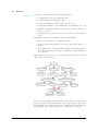
Definition 4.3:
A parameter graph is a directed, acyclic graph that represents the parameter space. It consists of AND-Nodes and OR-Nodes and edges between
them. Edges are directed and allowed only between different types of
nodes. OR-Nodes can have multiple incoming edges, while AND-Nodes
can only have exactly one incoming edge. Additionally edges have a
group number which is 0 if the edge doesn’t belong to any group. Parameter graphs have a single unique AND-Node without any incoming
edges. This node will be referred to as start node.
Definition 4.4:
OR-Nodes have a reference to a parameter.
20
EDACC User Guide
Definition 4.5:
AND-Nodes have a domain and a parameter reference to the same parameter as the preceding OR-node. AND-Nodes partition the possible
values of the parameter that they (and the preceding OR-node) reference. The domain of an AND-Node has to be a subset of the domain of
the preceding OR-Node.
The general idea is that the parameter space is specified by following the
structure of the graph from the start node and constraining the parameters using the domains encountered on the nodes. AND-Nodes imply
that all outgoing edges have to be followed while OR-Nodes mean that
exactly one edge has to be followed.
More formally:
Definition 4.6:
A solver configuration is valid if the start node (an AND-Node) of the
parameter graph is satisfied. Satisfied means:
1. an AND-Node is satisfied if the corresponding parameter value lies
in its domain and all OR-nodes adjacent via ungrouped edges are
satisfied.
2. an OR-Node is satisfied if exactly one adjacent AND-Node is satisfied and for at least one set of incoming edges with common group
number the preceding AND-Nodes are all satisfied.
EDACC User Guide
21
4.1
Example
Example 4:
Consider a solver that has the following parameters:
• c1 which takes on integer values in [1, 10].
• ps which takes on real values in [0, 1].
• A flag called lookahead which can be present or not.
• A categorical parameter steps which takes on values in {0, 1, 2, 3, 4}.
• Another categorical parameter method whose value is either ”hybrid” or ”atom”.
• A parameter prob which can be left out or take on real values in
[0, 1].
Furthermore there are some restrictions and requirements:
• Both c1 and ps have to be always specified.
• If the lookahead flag is present, both steps and method have to be
present.
• If steps takes on the value 0 and method takes on the value ”hybrid”,
then the parameter prob can take on values in its real domain [0, 1]
or be left out.
This parameter space can be encoded in a parameter graph as defined
earlier in the following way:
&
|| c1 Int[0,10]
|| ps Real[0,1]
& Int[0,10]
& Real[0,1]
|| steps Categ{0,1,2,3,4}
& Categ{1,2,3,4}
& Categ{0}
|| lookahead Flag
& <On>
& <Off>
|| method Categ{hybrid,atom}
& Categ{hybrid}
& Categ{atom}
|| prob Mix{Optional,
Real[0,1]}
&
<unspecified>
& Real[0,1]
The two red edges imply the membership of the edges to the same edge
group 6= 0. Black edges mean that the edge doesn’t belong to any group.
For simplicity, the parameter references of AND-Nodes (to the same parameter as the preceeding OR-Node) are not shown in the graph.
22
EDACC User Guide
5
5.1
Client
Introduction
The computation is client is used to compute the jobs of experiments.
Usually there have to be a lot of jobs computed to evaluate experiments
and since they are independent from each other, this task can be parallelized across many CPU cores. The computation client can be started on
arbitrarily many machines and will manage the available CPUs and start
jobs from the available experiments. It connects to the central database
and downloads all required resources such as instances and solver binaries
and writes back the results to the database.
5.2
System requirements
The client is written in C/C++ and should be able to run on most Linux
distributions where a MySQL C connector library is available.
TCP/IP Connections:
Connection alternatives:
Example 5:
Because the central storage location for all required computational ressources,
experiment metadata and results is a MySQL database, the client has to
be able to establish a connection to the machine that hosts the database.
This means that the machines where the client runs on have to be able
to establish a TCP/IP connection to the database machine.
The client was mainly tested on the bwGRID1 , a distributed computer
cluster that consists of several hundred nodes at several physical locations at universities of Baden-W¨
urttemberg, Germany. Even though the
machine hardware is homogenous, the network topology of bwGRID is
not. In cases where direct network access from the computation nodes
back to the database server is not possible it is usually possible to tunnel
a connection over the cluster’s login node back to the database via SSH.
For example running
ssh -f -N -L 0.0.0.0:1234:databasehost:3306 user@databasehost
on the login node sets up a tunnel for connections at port 1234 and
forwards them to your database machine at port 3306, where MySQL
listens. The options -f and -N will let the tunnel continue to run in the
background, even after logging out from the login node. To terminate
the tunnel, simply run e.g. killall ssh on the login node. In the client
configuration (see below), you would then specify the IP/hostname of the
login node and port 1234 as the database hostname and port.
Other than that, the client has to be able to write temporary files to some
location on the filesystem. This can be configured (5.3.1) if it differs from
the client binary location.
Shared filesystems:
Because the client will download missing solver binaries and instances
and upload results it also needs a reasonably fast network connection to
the database. Shared filesystems can considerably reduce the required
bandwidth since every file is only downloaded once. Alternatively you can
create a package from within the GUI that contains all solver binaries and
instances of an experiment. However, if you modify experiments while
the client is running it will still download missing files.
1
EDACC User Guide
http://www.bw-grid.de/
23
5.3
5.3.1
Usage
Configuration
Configuration file:
Example 6:
Configuration is done by some command line arguments and a simple
configuration file, called ”config”. This file has to be in the working
directory of the client at runtime. In the configuration file you have
to specify the database connection details and which hardware the client
runs on. This is done by configuring so called ”grid queues” in the GUI
application. They contain some basic information about the computation
hardware such as number of CPUs per machine. The client will then use
this information to run as many parallel jobs as the grid queue information allows it on each machine where it is launched. Here is a sample
configuration file:
host = database.host.foo.com
port = 3306
username = dbusername
password = dbpassword
database = dbname
gridqueue = 3
jobserver_host = jobserver.host.foo.com
jobserver_port = 3307
Note that the gridqueue value is simply the ID of the grid queue.
Command line arguments:
Beside the configuration file there are several command line options the
client accepts, please also see ”./client –help”:
-v <verbosity>:
Integer value between 0 and 4 (from lowest to
highest verbosity)
-l:
If flag is set, the log output is written to a file
instead of stdout.
-w <wait for jobs time (s)>:
How long the client should wait for jobs after
it didn’t get any new jobs before exiting.
-i <handle workers interval ms>:
How long the client should wait after handling
workers and before looking for a new job.
-k:
Whether to keep the solver and watcher output files after
uploading to the DB. Default behaviour is to delete them.
-b <path>:
Base path for creating temporary directories and files.
-d <path>:
Download path for resources. If the download path is a shared filesystem,
all clients with access to it will only need to download files once and t
copy them to their own base path.
-h:
Toggles whether the client should continue to run even
though the CPU hardware of the grid queue is not homogenous.
-s:
Enables simulation mode where the client will fetch and run
jobs but won’t write any results back to the database.
-t:
Expects walltime in the format [[[d:]h:]m:]s, you can let the client
24
EDACC User Guide
know how long it will be able to run on the system. The expected time lef
will then also show up in the GUI.
Verbosity controls the amount of log output the client generates. A value
of 4 is only useful for debugging purposes, a value of 0 will make the
client log important messages and all errors.
If the ”l” flag is set, log output goes to a file whose name includes the
hostname and IP address of the machine the client runs on. This is done
to avoid name clashes in shared filesystems typically found in computer
clusters. Otherwise log output goes to standard output.
With the ”-w” option you can tell the client how long to wait before
exiting after it didn’t start any jobs. This can be useful to keep the clients
running and ready to process new jobs while you evaluate preliminary
results and add new jobs or whole experiments. The wait option is also
used to determine how long attempts should be made to reconnect to the
database after connection losses. The default value is 10 seconds.
The ”-i” option controls how long the client should wait between its
main processing loop iterations. If this value is low, it will look for new
jobs when there are unused CPUs more frequently. For maximum job
throughput this value should be lower than the average job processing
time but lower values will also put more strain on the database and
increase the client’s CPU usage. The default value is 100ms which should
work fine in most cases. The client will also adapt to situations where
there are free CPUs but no more jobs and increase the interval internally
and fall back to the configured value once it got another job.
The ”-k” flag tells the client that it should keep temporary job output
files after a job is finished. The default behaviour is to delete them.
The ”-b” base path option can be used to specify a directory the client
can use to write temporary files to. The default value is ”.”, i.e. the
working directory at runtime.
inhomogenous machines
The first client to start with a particular grid queue will write the in-
! → formation about the machine it runs on to the grid queue entry in the
database. All following clients will then compare their machines to the
information in the grid queue and exit, unless the number of cores and
the CPU model name match. With the ”-h” option you can override this
behaviour.
5.3.2
Launching
After configuration you can simply run the client on your computation
machines. On computer clusters there are often queuing systems that
you have to use to gain access to the nodes. On bwGRID for example,
we could use the following short PBS (portable batch script) and submit
(qsub scriptname) our client to a node with 8 cores:
#!/bin/sh
#PBS -l walltime=10:00:00
#PBS -l nodes=1:ppn=8
cd /path/to/shared/fs/with/client/executable
./client -v0 -l -i200 -w120
! → You should always run the client from within its directory (i.e. cd to the
directory) to avoid problems with relative paths such as the verifier path
from the example configuration above.
EDACC User Guide
25
As soon as clients start you should be able to see jobs changing their
status from ”not started” to ”running” in the GUI’s or Web frontend’s
job browsers.
5.3.3
Troubleshooting
If errors or failures occur the client will always attempt to shut down
cleanly, that is stop all running jobs and set their status to ”client
crashed” and write the last lines of its log output as ”launcher output”
to each job. This can fail when network connections fail or the client
receives a SIGKILL signal causing it to exit immediately. In case of network failures you should still be able to find useful information in the
client’s logfile on the local filesystem.
5.4
Verifiers
Verifiers are programs that the client runs after a job finishes. Verifiers
are getting passed the instance of the job and the solver output as arguments and are supposed to write a newline character followed by a
(textual/ASCII) integer result code at the end of their output. The result code should convey some information about the result of the job, for
example whether the output of the solver is correct given the problem
instance. This code will be written to the database as ”result code” while
the verifier’s exit code will be written as ”verifier exit code”. Any output
the verifier writes to standard out will be written as ”verifier output”.
The call specification for a verifier binary looks like this:
./verifier_binary <path_to_instance> <path_to_solver_output>
! →
5.5
We provide a verifier for the SAT problem that works on CNF instances
in DIMACS format and solvers that adhere to a certain output format
(see the source code). If you want to write an own verifier specific to
your problem you can also use the source code as implementation example. Note that you have to make sure that your possible result codes are
specified in the ResultCodes table in the database before running clients
or there will be errors when the client tries to write results. By convention, the web frontend and GUI application consider result codes that
begin with a decimal ”1” as correct answers.
Experiment priorization
Sometimes it can be useful to compute several experiments in parallel
but give some a higher priority than others. In order to accomplish
that, experiments can be marked as inactive and individual jobs can be
prioritized. Only jobs of active experiments with priority equal to or
greater than 0 are considered for processing by the client. Futhermore,
experiments can be assigned a priority. The clients will then try to match
the relative number of CPUs working on an experiment with its relative
priority to all other experiments that are assigned to the same grid queue.
For example, if you have three experiments with priorities 100, 200 and
300 respectively the running clients will try to have 16% of CPUs working
on the first, 33% of CPUs working on the second and 50% of CPUs
working on the third experiment.
26
EDACC User Guide
! → The client is running solely on Unix and is not distributed yet for Windows systems.
EDACC User Guide
27
6
6.1
Web Frontend
Introduction
The Web Frontend provides access to experiment information and analysis tools in a read-only manner and accessible by a web browser.
6.2
System requirements
The web frontend is implemented as Python WSGI web application and
makes use of several libraries. Since it interfaces with R to draw plots
it also depends on R and a Python interface to R, which unfortunately
only works properly on Linux right now. WSGI applications can be
deployed on a variety of web servers or even run standalone on a web
server that comes with the Python standard library. The following list
contains all dependencies and prerequisites of the Web Frontend (see 6.3
for installation instructions).
• Python 2.6.5 or 2.7 http://www.python.org
• R 2.11 (language for statistical computing and graphics)
• R package ’np’ (available via R’s CRAN)
• SQLAlchemy 0.6.5 (SQL Toolkit and Object Relational Mapper)
• mysql-python 1.2.3c1 (Python MySQL adapter)
• Flask 0.6 (Micro Webframework)
• Flask-WTF 0.3.3 (Flask extension for WTForms)
• Flask-Actions 0.5.2 (Flask extension)
• Werkzeug 0.6.2 (Webframework, Flask dependency)
• Jinja2 2.5 (Template Engine)
• PyLZMA 0.4.2 (Python LZMA SDK bindings)
• rpy2 2.1.4 (Python R interface)
• PIL 1.1.7 (Python Imaging Library)
• Numpy 1.5.1
• pygame 1.9 (Graphics library)
6.3
Installation
To get rpy2 working the GNU linker (ld) has to be able to find libR.so.
Add the folder containing libR.so (usually /usr/lib/R/lib) to the ld config: Create a file called R.conf containing the path in the folder /etc/ld.so.conf.d/
and run ldconfig without parameters as root to update. Additionally, you
have to install the R package ’np’ which provides non-parametric statistical methods. This package can be installed by running ”install.packages(’np’)”
within the R interpreter (as root).
Example 7:
The following installation example outlines the step that have to be taken
to install the web frontend on Ubuntu 10.04 running on the Apache 2.2.14
web server. For performance reasons (e.g. query latency) the web frontend should run on the same machine that the EDACC database runs
on.
1. Install Apache and the WSGI module:
28
EDACC User Guide
apt-get install apache2 libapache2-mod-wsgi
2. Copy the web frontend files to /srv/edacc web/, create an empty
error.log file and change their ownership to the Apache user:
touch /srv/edacc_web/error.log
chown www-data:www-data -R /srv/edacc_web
3. Create an Apache virtual host
(new file at /etc/apache2/sites-available/edacc web)
<VirtualHost *:80>
ServerAdmin [email protected]
ServerName foo.server.com
LimitRequestLine 51200000
WSGIDaemonProcess edacc processes=1 threads=15
WSGIScriptAlias / /srv/edacc_web/edacc_web.wsgi
Alias /static/ /srv/edacc_web/edacc/static/
<Directory /srv/edacc_web>
WSGIProcessGroup edacc
WSGIApplicationGroup %{GLOBAL}
Order deny,allow
Allow from all
</Directory>
<Directory /srv/edacc_web/edacc/static>
Order allow,deny
Allow from all
</Directory>
</VirtualHost>
4. Install dependencies and create a virtual environment for Python
libraries:
apt-get install python-pip python-virtualenv python-scipy
apt-get install python-pygame python-imaging
virtualenv /srv/edacc_web/env
apt-get build-dep python-mysqldb
apt-get install r-base
echo "/usr/lib/R/lib" > /etc/ld.so.conf.d/R.config
ldconfig
source /srv/edacc_web/env/bin/activate
pip install mysql-python
pip install rpy2
pip install flask flask-wtf flask-actions
pip install sqlalchemy pylzma numpy
5. Install R libraries (”R” launches the R interpreter):
R
install.packages(’np’)
6. Create a WSGI file at /srv/edacc web/edacc web.wsgi with the following contents:
import site, sys, os
site.addsitedir(’/srv/edacc_web/env/lib/python2.6/site-packages’)
EDACC User Guide
29
sys.path.append(’/srv/edacc_web’)
sys.path.append(’/srv/edacc_web/edacc’)
os.environ[’PYTHON_EGG_CACHE’] = ’/tmp’
sys.stdout = sys.stderr
from edacc.web import app as application
7. Configure the web frontend by editing /srv/edacc web/edacc/config.py,
see 6.4 for details.
8. Enable the Apache virtual host created earlier:
a2ensite edacc_web
service apache2 restart
9. The web frontend should now be running under http://foo.server.com/
6.4
Configuration
! →
Database configuration
6.5
All configuration is done in a Python file located at ”edacc/config.py”.
The options are documented in the sample configuration file which is included in the distribution package. Please read through the configuration
options and modify those marked as important. Most importantly, you
should disable debugging mode and change the secret key when making
the Web Frontend accessible from the network to avoid security problems. Logging is also quite useful to make it easier to find the cause
of bugs in the application. At the end of the file you can configure the
database connection and the list of EDACC databases that should be
made available by the Web Frontend.
Troubleshooting
When there are errors or bugs and you have set up the Web Frontend
under Apache as described in the installation section, Apache will display
an ”Internal Server Error” page. If you have configured logging, the
application will write tracebacks to the logging file. If you haven’t set up
logging, these tracebacks will end up in Apache’s error.log file.
6.6
Features
This section gives a short overview of the features of the Web Frontend.
Most features should be self-explanatory or have some additional documentation on the pages themself.
The Web Frontend was designed as monitoring and analysis tools of experiments that are created with the GUI application. Once you have
set up some databases and added them to the configuration file of the
Web Frontend, the top level page will allow the user to select one of
the databases. This leads to a page that displays all experiments of the
chosen database and some basic information about their creation date,
number of solvers, instances and jobs.
30
Experiments
An experiment page displays further information about the experiment,
such as the number of total, running and crashed jobs. If the experiment
is currently being computed, an estimation of the time of completion is
displayed next to ”ETA”.
Monitor progress
Under ”Progress” a colored bar visualizes the computation progress.
Green color corresponds to finished jobs, red to crashed jobs and orange to jobs that are currently being computed. The links following the
progress bar lead to information and analysis pages.
EDACC User Guide
Figure 1: Live result browser showing the jobs of an experiment on SAT
solvers. The ”Flips” result property column contains the values of the
number of local search steps performed by the solver.
Job browser
Export data
Download instances
View results
Export results
Analyse results
Export plots
The progress page provides a job browser similar to the GUI application.
It allows to sort, filter for certain words, show and hide specific columns
and download currently displayed data in CSV (comma-separated values)
format. Displaying more than 1000 results at once can become rather
slow, since the browser’s Javascript engine has to do a lot of processing
to color and format the table.
The solver configurations and instances pages show the solver configurations and instances that are part of the experiment. The instances page
provides a download link for all instance files in a tarball. Instances are
shown in a table by name, MD5 checksum and their properties , if there
are any. The instance name links to a page that displays the first and
last few characters of the instance file and provides a download link.
The result pages display the results of the jobs in various formats. ”Unsolved instances” and ”Solved instances” list the instances that were not
solved by any solver or solved by at least one solver respectively. ”By
solver configuration” leads to a page, where after selecting a solver configuration that is part of the experiment a table is displayed containing
all the results of the jobs of the solver configuration by instance and run
number. ”By instance” leads to a page, where after selecting an instance
all results obtained on this instance are displayed by solver configuration
and run number. All tables can be exported (i.e. downloaded) in CSV
format.
Analysis pages provide various plots of results and statistical tools such
as correlation and probabilistic domination calculations. All plots can
be directly saved in PNG format as they are displayed in the browser
or downloaded in PDF or EPS format. For some plots the application
generates an R script which can be adjusted as neccessary. Most plots
allow to download the underlying data in CSV format.
Some plots allow the selection of multiple instances. In this case, you can
use a filter to narrow the selection of the instances listed. Please refer to
the example which is displayed next to the filter text field.
Ranking of solver
configurations
EDACC User Guide
The ranking is determined by the number of successful runs but the
ranking table can be sorted by any of the displayed measures.
31
6.7
Result pages
The main web page gives a list of experiments that are in the database
along with information about the experiment’s date, number of solver
configurations, instances and attempts. Each experiment in the list links
to a web page that provides links to various web pages with further
information, results and analysis tools.
The Live information about experiment progress page displays a table of
the experiment’s jobs in rows with several columns for the attributes of a
job. By default, the unique ID of a job, its solver configuration, instance
and run number, run time, seed, status and result code in textual form,
are displayed. Additionally, for each result property in the database
there’s a column with the property value of the job, if it was already
calculated and is present in the database. The job data is retrieved from
the database on each page refresh and directly reflects the computation
progress of an experiment. Aside from browsing the table, which includes
sorting and filtering for some of the columns, the table data can also be
downloaded in CSV format2 for processing with other tools. The ID is
also a link that leads to a detailed result page for the job. This page
displays links to the solver configuration and instance of the job and the
values of all result properties, if they are calculated. The solver, launcher,
watcher and verifier output is displayed as well but each truncated to a
reasonable size, only showing the first and last few hundred characters.
Links allow the user to download the entire files.
The ”list of solver configurations used” page displays the list of solver
configurations that are part of the experiment. For each solver configuration a page with details about the solver and the arguments can be
accessed. The ”list of instances used” page displays the list of instances
used in the experiment in a table. There are columns for the name, md5
checksum and additional columns for each instance property defined in
the database. Each instance has a link to a page that displays the first
and last few hundred characters of the instance file and allows to download the entire file.
There are three pages that display the results of an experiment in different
formats:
1. By solver configuration: Allows the user to select a solver configuration and then displays a table with the solver configuration’s run
time results of all attempts on the instances of the experiment. The
results are links to the detailed result pages of the corresponding
jobs.
2. By instance: Allows the user to select an instance and then displays a table with the run time results of all attempts of the solver
configurations of the experiment.
3. By solver configuration and instance: Displays a table with the
instances of the experiment as rows and the solver configurations
as columns. If there’s only one attempt for each solver on an instance, the cell corresponding to a particular solver configuration
and instance displays the run time of the single attempt and it’s
result code in textual form. If there are multiple attempts, each cell
contains descriptive statistics such as the median, minimum, maximum and average run time, as well as its standard deviation, over
2
32
comma-separated values
EDACC User Guide
Number of solved instances within a given amount of CPU time
Sparrow
TNM
gNovelty+2
adaptG2WSAT2009++
100
CPU Time (s)
80
60
40
20
0
0
50
100
150
number of solved instances
Figure 2: Cactus plot
all attempts. A link in each cell leads to a table with the results of
all attempts.
The data of the tables displayed in the two result pages mentioned first
can be downloaded in CSV format.
6.8
Analysis pages
The statistical methods implemented were described in chapter ?? in
detail. In the web frontend they are made available on pages that are
accessible from an experiment’s main page. Each has a form that allows
the user to set the parameters of the plots and tests, for example which
solver configurations and instances to include. After submitting the form
the pages display the results of the tests or the plots. The following tests
and plots are implemented in the web frontend:
• Box plots: The form allows the selection of the result property and
the solver configurations and instances of which the results should
be plotted. After submitting the form the box plot is displayed.
• Scatter plot - One result property of two solvers: The form allows
the selection of the two solver configurations, the instances and
whether to plot single runs, all runs or average or median values.
• Scatter plot - Two result properties of a solver: The form allows the
user to select the solver configuration, the instances and whether
to plot single runs, all runs or average or median values.
• Scatter plot - Result property against instance property: A form
allows to select the solver configuration, result property, instance
property and whether to plot single runs, all runs or average or
median values.
EDACC User Guide
33
• Distribution and Kernel Density Estimation: After selecting the
solver configuration, instance and result property the plots of the
empirical distribution function and the kernel density estimation
are displayed.
• Property distribution comparison of two solvers on an instance: A
form allows to select two solver configurations, the instance and
the result property. After submitting the form data, a plot of both
property distributions and the results of the two hypothesis tests
described in the last chapter are displayed. For both tests, the
null hypothesis, the alternative hypothesis, the test statistic, the pvalue and the conclusion about whether to accept or reject the null
hypothesis at significance level 0.05 are calculated and displayed.
• Property distributions of solvers on an instance: After selecting
several solver configurations, an instance and a result property, the
result property distributions are displayed in a single plot.
• Cactus plot: Cactus plots show the number of attempts a solver
configuration would be able to finish successfully if it is restricted
to a certain amount of a result property on every attempt. For
example, the number of successful runs if given a certain amount
of time (see Figure 2).
• Probabilistic domination: After selecting two solver configurations
and a result property the instances are split into the three categories
of probabilistic domination as described in chapter ??.
The Pearson product-moment correlation coefficient and Spearman’s rank
correlation coefficient are calculated for the data of the scatter plots
and displayed next to them. All plots are rendered in PNG3 format for
presentation on the web pages and can be downloaded by the user as
PDF and EPS4 images for further use. Additionally, the numeric data
that is used to generate the plots can be downloaded in CSV format.
3
4
34
Portable Network Graphics
Encapsulated Postscript
EDACC User Guide
7
Automatic Algorithm Configuration
8
Monitor
9
Troubleshooting
EDACC User Guide
35
Index
Algorithm engineering, 3
Analysis, 31
Client configuration, 24
Computation progress, Web Frontend, 30
Configuration Experiment, 14
Configuration Scenario, 14
Configuration, Web Frontend, 30
create/remove/edit experiments, 12
DB Model upgrade, 7
Experiment, 12
Export plots, 31
Export results, 31
Generate Cluster Package, 17
Generate Jobs, 16
Generate Solver Configurations, 15
Grid Queue, 17
Grid queue, 24
GUI update, 7
Installation, Web Frontend, 28
Instance, Seed-Course, 15
Instances tab, 16
Plots, 31
Queue Selection, 17
Ranking, 31
Result Code, 12
Results, 31
select instances, 16
Shared filesystems, 23
Solver, 8
Solver authors, 8
Solver binaries, 8
Solver code, 8
Solver configuration, 15
Solver description, 8
Solver name, 8
Solver version, 8
Statistical tools, 31
System requirements client, 23
System requirements, Web Frontend, 28
Troubleshooting, Web Frontend, 30
Visualization, 31
Web Frontend, 28
36
EDACC User Guide