Download Toro Aqua-Traxx with the PBX Advantage Design Guide

Aqua-TraXX
Design Manual
By Michael J. Boswell

This publication is designed to provide accurate and informative opinion in regard to
the subject matter covered. It is distributed with the understanding that the authors,
publishers, and distributors are not engaged in rendering engineering, hydraulic,
agronomic, or other professional advice.
Printing History:
First Edition
Second Edition
Third Edition
Fourth Edition
June 1997
August 1998
October 1999
August 2000
 Toro Ag Irrigation 2000
TABLE OF CONTENTS
CHAPTER I:
Aqua-TraXX TAPE
Principles of Operation
Features and Advantages
Specifications
Use and Selection
CHAPTER II:
SOIL
Soil
CHAPTER III:
WATER QUALITY AND TREATMENT
Water Quality
Water Treatment
Chlorination
Injection of Acid
CHAPTER IV:
DESIGN CRITERIA
Emission Uniformity (EU)
Design Capacity
CHAPTER V:
Aqua-TraXX DESIGN
Selecting Aqua-TraXX Products
Computer Program AquaFlow
Submain Design
Mainline Design
CHAPTER VI:
INSTALLATION PROCEDURES
Installation
Connections
Injection Equipment
CHAPTER VII: OPERATION AND MAINTENANCE
Computing Irrigation Time
Monitoring System Performance
Maintenance Procedures for Aqua-TraXX Tape
APPENDIX A: CONVERSION FACTORS
APPENDIX B: REFERENCE TABLES OF SELECTED DATA
LIST OF FIGURES:
Figure 1:
Figure 2:
Figure 3:
Figure 4:
Figure 5:
Figure 6:
Figure 7:
Figure 8:
Figure 9:
Figure 10:
Figure 11:
Figure 12:
Figure 13:
Figure 14:
Figure 15:
Figure 16:
Figure 17:
Aqua-TraXX Tape
Aqua-TraXX on Lettuce (Murcia, Spain)
Turbulent Flowpath Design Details
Aqua-TraXX on Tomatoes (Florida sandy soil)
Wetting Patterns for Clay, Loam, and Sand
Effect of Emitter Location on Salts
Aqua-TraXX on Head Lettuce (Santa Maria, CA)
Aqua-TraXX on Broccoli (Santa Maria, CA)
Screen Mesh Sizes Compared to 0.020” Orifice
Aqua-TraXX on Celery (Santa Maria, CA)
Aqua-TraXX on Strawberries (Dover, Florida)
Example Submain Block
Aqua-TraXX Connection to Oval Hose
Methods of Aqua-TraXX Tape Connections
Injecting Aqua-TraXX (Casa Grande, Arizona)
Aqua-TraXX Injection Tool
Aqua-TraXX on Peppers (Florida sandy soil)
1-1
1-2
1-3
2-1
2-3
2-4
3-1
3-5
3-7
4-2
5-1
5-4
6-2
6-2
6-3
6-5
7-1
LIST OF TABLES:
Table 1:
Table 2:
Table 3:
Table 4:
Table 5:
Approximate Size of Wetted Area
Water Quality Interpretation Chart
Chlorine Equivalents for Commercial Sources
Standard Flow Rates for Aqua-TraXX
Friction Losses in PSI through Tape Connections
2-3
3-3
3-13
5-2
6-3
LIST OF EQUATIONS:
Eq. 1:
Eq. 2:
Eq. 3:
Eq. 4:
Eq. 5:
Eq. 6:
Eq. 7:
Chlorine Injection Rate (Liquid Form)
Chlorine Injection Rate (Gas Form)
Emission Uniformity – EU
Peak Evapotranspiration – PET
Friction Loss in Pipe Equation
Velocity in Pipe Equation
Irrigation Time
3-11
3-12
4-1
4-4
5-12
5-12
7-1
CHAPTER I
Aqua-TraXX TAPE
PRINCIPLES OF OPERATION
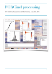
Aqua-TraXX is a seamless, extruded drip tape with a molded, turbulent flow emitter
bonded to the inner wall.
Seamless construction eliminates seam failures, and reduces the incidence of root
intrusion. Extrusion technology utilizes high-quality, extrusion-grade engineering
polymers renowned for their toughness and flexibility. These polymers were
developed specifically for use in harsh industrial and agricultural environments.
The exclusive flowpath molding process creates crisp, well-formed physical features,
resulting in excellent repeatability and high emission uniformity (EU). The
turbulent flowpath design creates a clog-resistant flow channel, and permits longer
run lengths and higher uniformity of water application.
As shown in Fig. 1, water enters the flowpath through the filter inlets, and then flows
through the turbulent flow channel which accurately regulates the flow rate. Finally,
the water flows through the laser-made, slit type outlets to the crop.
Figure 1: Aqua-TraXX Tape
Chapter I: Aqua-TraXX Tape
1-1
FEATURES AND ADVANTAGES
⇒ Precision molded emitter for high uniformity.
⇒ Seamless construction for greater reliability.
⇒ Each flowpath has many filter inlets, making it highly resistant to clogging.
⇒ Laser slit outlet eliminates startup clogging and impedes root intrusion.
⇒ Truly turbulent flowpath provides excellent uniformity with reduced clogging.
⇒ Available in a wide range of wall thicknesses, outlet spacings and flow rates.
⇒ Highly visible blue stripes for quality recognition and Emitter UP indicator.
⇒ Superior tensile and burst strength.
⇒ Tough, abrasion-resistant material reduces field damage.
⇒ East and West Coast manufacturing for prompt delivery and enhanced
availability.
Figure 2: Aqua-TraXX on Lettuce (Murcia, Spain)
1-2
Chapter I: Aqua-TraXX Tape
SPECIFICATIONS
Aqua-TraXX Diameter & Wall Thickness Dimensions
Diameter
5/8”
7/8”
1-3/8”
Wall (mils)
4
6
8
10
12
15
8
10
12
15
Min PSI
4
4
4
4
4
4
4
4
4
4
Max PSI
10
12
15
15
15
15
15
15
15
15
Reel Length
13,000’
10,000’
7,500’
6,000’
5,100’
4,000’
6,000’
4,400’
4,000’
2,700’
Reel Weight
70 lbs
66 lbs
63 lbs
60 lbs
58 lbs
61 lbs
68 lbs
65 lbs
61 lbs
74 lbs
Flowpath Specifications & Dimensions
Number of Inlets
Number of Inlets
Inlet Dimensions
Flowpath Dimensions
Outlet Dimensions
Outlet Dimensions
Coefficient of Variation
Flow Coefficient Cd & X
Flow Coefficient Cd & X
Flow Coefficient Cd & X
Flow Coefficient Cd & X
Hazen-Williams C Factor
8” & 16” spacing
12” & 24” spacing
(All)
(All)
4 & 6 mil
8 - 15 mil
(All)
Cane Flow (6 - 12 psi range)
High Flow (6 - 12 psi range)
Med Flow (6 - 12 psi range)
Low Flow (6 – 12 psi range)
(Main Tube)
60
200
.007 min. x .010 max.
.008 min. x .033 max.
.140 x .012
.170 x .012
0.03
0.11859, 0.50
0.09487, 0.50
0.07115, 0.50
0.04743, 0.50
140
Flowpath Design & Nomenclature
Figure 3: Turbulent Flowpath Design Details
Chapter I: Aqua-TraXX Tape
1-3
USE AND SELECTION
Wall Thickness
4 mil - Light-walled products used for short season crops, in soils with a minimum of
rocks. Recommended for experienced tape users.
6 and 8 mil - Intermediate products for general use in longer-term crops and average
soil conditions.
10 -15 mil - Heavy wall designed to be used in rocky soils, where insects and animals
may cause damage, or where the tape is to be used for more than one season.
Spacing
8 inch - Used in closely spaced crops, on sandy soils, or where higher flow rates are
desired.
12 inch - Used on crops in medium soils and average crop spacings.
16 inch - Used on wide spaced crops where a longer length of run is desired.
24 inch - Used for widely spaced crops, heavy soils, long run lengths.
Flow Rate
Cane Flow – Used for sugarcane.
High Flow - Normally recommended for most crops and soils.
Medium Flow - Recommended for longer runs on most crops and soils.
Low Flow - Used in soils with low infiltration rates, where long irrigation times are
necessary, or for very long runs.
Diameter
5/8” - Used for average run lengths (0 to 1,000 ft).
7/8” - Used for long run lengths (up to 2,500 ft).
1-3/8” - Used for very long run lengths (up to 5,000 ft).
1-4
Chapter I: Aqua-TraXX Tape
CHAPTER II
SOIL
SOIL
Soil Water Relationships
A micro-irrigation system is a transportation system that delivers water to a point in
or near the root zone. The final link in this transportation system is the soil, an
essential bridge between the irrigation system and the plant. The soil's physical and
chemical properties determine its ability to transport and store water and nutrients.
The characteristics of soils vary widely according to their physical properties, often
determining the type of crop that can be grown, and the type of irrigation system that
is appropriate. Therefore, a thorough understanding of soil properties and soil-water
relationships is important for purposes of irrigation design.
Figure 4: Aqua-TraXX on Tomatoes (Florida sandy soil)
Chapter II: Soil and Water Quality
2-1
Infiltration Rate
The infiltration rate is the rate at which water enters the soil. A soil's infiltration rate
will vary greatly according to its chemistry, structure, tilth, density, porosity, and
moisture content. The infiltration rate of a soil may impose a limitation upon the
design of an irrigation system, since water application rates in excess of the
infiltration rate may result in runoff and erosion.
Soil Water Movement
When water is applied slowly to the soil at a single point, it is acted upon by the
forces of gravity (downward) and capillary action (radially outward), producing a
wetted pattern characteristic of the soil type and application rate.
Sandy soils are characterized by large voids between soil particles. These large voids
exert relatively weak capillary forces, but offer little resistance to gravitational flow,
with the result that lateral and upward water movement is limited, while downward
water movement is rapid. The wetting pattern for a sandy soil will therefore be deep
with little lateral spread, and upward water movement will be minimal. To improve
the lateral distribution of water on sandy soils, some Florida tomato growers have
installed two Aqua-TraXX rows per bed, as shown in Figure 4.
At the other extreme, a heavy clay soil exerts strong capillary forces, but resists
downward water movement by gravity. The wetted pattern in a heavy clay soil will
tend to be broad and of moderate depth because of the clay's high capillary forces and
relatively low permeability. In clay soils which have undergone compaction, the
downward movement of the water is even further restricted, resulting in a wetted
zone that is wide and shallow. In clay soils the wetted pattern will depend not only
on soil type, but will also vary markedly with the tilth of the soil.
For the majority of soils, wetting patterns will be between the extremes exhibited by
light sands and heavy clays. In addition, water movement in soils will be affected by
the condition of the topsoil, the permeability of the subsoil, layers of soil with
varying properties, and the presence of a plow pan. Figure 5 illustrates the relative
shapes of wetting patterns that might be created under a tape outlet in various soil
types.
2-2
Chapter II: Soil and Water Quality
Figure 5: Wetting Patterns For Clay, Loam And Sand
Application Rate
In addition to soil type, the application rate will affect the shape of the wetted pattern.
It is possible to alter the shape of the wetted zone by varying the application rate. For
example, 10 gallons of water applied to a soil in 1 hour will probably produce a
wider, shallower wetted pattern than 10 gallons applied over a 10-hour period. This
is because a higher application rate tends to produce a wider zone of saturation under
the emitter, assisting horizontal movement.
For increased lateral movement, light sandy soils require water application at higher
rates. Heavy clays and clay loams, on the other hand, often benefit from a lower
water application rate. This low rate avoids surface ponding and runoff, and
promotes deeper water penetration. Table 1 provides data on the approximate size of
the wetted area, which can be expected under average conditions.
Table 1: Approximate Size of Wetted Area
SOIL TYPE
Coarse Sand
Fine Sand
Loam
Heavy Clay
Chapter II: Soil and Water Quality
WETTED RADIUS (ft)
0.5 - 1.5
1.0 - 3.0
3.0 - 4.5
4.0 - 6.0
2-3
Tape Placement In Relation To The Plant
Tape placement is an important factor in the performance of the irrigation system and
the health of the crop. The location of the tape in relation to the plant will affect
germination and early growth, establishment of the root system, efficient utilization
of water and nutrients, and the effects of salinity on the plant.
Germination of seeds or initial growth of seedlings will usually require that the tape
be placed in close proximity - 18 inches or less in most soils - to the plant. In sandy
soils this distance should be reduced to 12 inches or less.
The outlet spacing, flow rate and location of the tape will establish the wetted zone,
and therefore the location of most intensive root development. The root system can
be encouraged to extend itself horizontally or vertically, or it can be confined to a
relatively small area. The size and shape of the root system is important in terms of
the stability and vigor of the plant, and its ability to utilize the naturally occurring
water and nutrients in the soil around it. Because water and nutrients applied outside
the confines of the root zone are wasted, it is best to locate the tape near the center of
the root zone.
Salts present in the soil or in the irrigation water will be concentrated at the perimeter
of the wetted zone formed around the tape, as shown in Figure 6. The placement of
the tape will determine whether harmful salts are pushed out and away from the root
zone, or concentrated within it.
Figure 6: Effect Of Emitter Location On Salts
2-4
Chapter II: Soil and Water Quality
Determination of Wetting Pattern
The wetting pattern for any given soil is difficult to predict accurately from
knowledge of the soil type alone. General principles may be outlined, but for
practical purposes, a test of the wetting pattern should be carried out on the proposed
site of the irrigation system.
Much can be learned about water movement by applying measured amounts of water
to limited areas and observing the lateral and downward movement of water, and the
shape of the wetted zone at various time intervals. Provided that the soils tested are
representative, the observations will have practical application to the design of the
irrigation system. Such experiments can reveal soil layers and compaction zones,
and can indicate water retention capacities and the time needed for the soil to reach
field capacity at different depths in the soil.
A simple method for determining the wetting pattern in a particular soil consists of
installing a tape lateral of the type to be used, and connecting it to a temporary water
source such as an elevated 55-gallon drum. The drum is filled with water and the test
system is allowed to run for some length of time. Observations of the wetting pattern
are made by measuring the wetted surface diameter, and by digging beneath the
surface to measure the extent of subsurface water movement. This test will provide
extremely valuable information concerning wetting patterns and water movement in
the specific soil type of interest.
Chapter II: Soil and Water Quality
2-5
CHAPTER III
WATER QUALITY AND TREATMENT
WATER QUALITY
Taking A Water Sample For Analysis
The preliminary study for a micro-irrigation system will require a careful analysis of
the source water. A micro-irrigation system requires good quality water free of all but
the finest suspended solids and free of those dissolved solids, such as iron, which may
precipitate out and cause problems in the system. Neglecting to analyze the quality of
source water and provide adequate treatment is one of the most common reasons for
the failure of micro-irrigation systems to function properly.
Figure 7: Aqua-TraXX on Head Lettuce
It is important that a representative water sample be taken. If the source is a well, the
sample should be collected after the pump has run for half an hour or so. For a tap on a
domestic supply line, the supply should be run for several minutes before taking the
sample. When collecting samples from a surface water source such as a ditch, river, or
reservoir, the samples should be taken near the center and below the water surface.
Chapter III: Water Treatment
3-1
Where surface water sources are subject to seasonal variations in quality, these sources
should be sampled and analyzed when the water quality is at its worst.
Glass containers are preferable for sample collection and they should hold about a halfgallon. The containers should be thoroughly cleaned and rinsed before use to avoid
contamination of the water sample. Two samples should be collected. The first sample
should be used for all tests except iron, and no additives are required. The second
sample is used for the iron analysis, and after collecting the water, ten drops of HCl
should be added. HCl is commonly available in the form of muriatic acid.
Sample bottles should be filled completely, carefully labeled, and tightly sealed.
Samples should be sent immediately to a water-testing laboratory. The following tests
should be requested from the laboratory: Salinity, pH, Calcium, Magnesium, Sodium,
Potassium, Iron, Manganese, Boron, Bicarbonate, Carbonate, Chloride, Sulfate,
Sulfide, the quantity and size of suspended solids and, for city water supplies, the free
chlorine level.
The water should also be tested for the presence of oil, especially in areas close to oil
fields. Oil will very rapidly block both sand media and screen filters. Oil may also clog
tape outlets and may attack plastic pipes, tubing, or other components.
Interpretation Of Water Quality Analysis
Suspended Solids
Suspended solids in the water supply include soil particles ranging in size from coarse
sands to fine clays, living organisms including algae and bacteria, and a wide variety of
miscellaneous waterborne matter. Suspended solids loads will often vary considerably
over time and seasonally, particularly when the water source is a river, lake, or
reservoir.
Calcium
Calcium (Ca) is found to some extent in all natural waters. A soil saturated with
calcium is friable and easily worked, permits water to penetrate easily and does not
puddle or run together when wet. Calcium, in the form of gypsum, is often applied to
soils to improve their physical properties. Generally, irrigation water high in dissolved
calcium is desirable, although under certain conditions, calcium can precipitate out and
cause clogging.
Iron
Iron (Fe) may be present in soluble form, and may create clogging problems at
concentrations as low as 0.1 ppm. Dissolved iron may precipitate out of the water due
3-2
Chapter III: Water Treatment
to changes in temperature, in response to a rise in pH, or through the action of bacteria.
The result is an ocher sludge or slime mass capable of clogging the entire irrigation
system.
Manganese
Manganese (Mn) occurs in groundwater less commonly than iron, and generally in
smaller amounts. Like iron, manganese in solution may precipitate out because of
chemical or biological activity, forming sediment, which will clog tape emitters. The
color of the deposits ranges from dark brown, if there is a mixture of iron, to black if
the manganese oxide is pure. Caution should be exercised when chlorination is
practiced with waters containing manganese, due to the fact that there is a time delay
between chlorination and the development of a precipitate.
Sulfides
If the irrigation water contains more than 0.1 ppm of total sulfides, sulfur bacteria may
grow within the irrigation system, forming masses of slime, which may clog filters and
tape outlets.
Interpreting The Water Analysis
Table 2 provides a guideline for interpretation of water analysis results.
Table 2: Water Quality Interpretation Chart
WATER QUALITY
PARAMETER
1. Salinity
EC (mmho/cm)
TDS (ppm)
2. Permeability
- Caused by Low Salt
EC (mmho/cm)
TDS (ppm)
- Caused by Sodium
SARa
3. Toxicity
Sodium (SARa)
Chloride (me/L)
(ppm)
Boron (ppm)
DEGREE OF PROBLEM
NONE
INCREASING
SEVERE
0.0 - 0.8
0.0 – 500
0.8 - 3.0
500 - 2,000
3.0 +
2,000 +
0.5 +
320 +
0.5 - 0.2
320 - 0.0
0.2 - 0.0
0.0 - 6.0
6.0 - 9.0
9.0 +
0.0 - 3.0
0.0 - 4.0
0.0 – 140
0.0 - 0.5
3.0 - 9.0
4.0 - 10.0
140 – 350
0.5 - 2.0
9.0 +
10.0 +
350 +
2.0 +
4. Clogging
Chapter III: Water Treatment
3-3
Iron (ppm)
Manganese (ppm)
Sulfides (ppm)
Calcium Carbonate (ppm)
0.0 - 0.1
0.0 - 0.2
0.0 - 0.1
0.1 - 0.4
0.2 - 0.4
0.1 - 0.2
0.4 +
0.4 +
0.2 +
No levels established
WATER TREATMENT
Micro-irrigation systems are characterized by large numbers of emitters having fairly
small flow paths. Because these small flow paths are easily clogged by foreign
material, many water sources require some treatment to ensure the successful longterm operation of the system. Nearly all water sources can be made suitable for
micro-irrigation by means of appropriate physical and/or chemical treatment.
The various water quality problems encountered in operating micro-irrigation
systems are outlined below. In some situations, two or more of these problems may
be present, giving rise to more complex treatment procedures.
1.
Presence of large particulate matter in the water supply.
2.
Presence of high silt and clay loads in the water supply.
3.
Growth of bacterial slime in the system.
4.
Growth of algae within the water supply or the system.
5.
Precipitation of iron, sulfur, or calcium carbonates.
Presence Of Large Particulate Matter
Large particles present in the water supply will usually be either inorganic sands or
silts, scale from pipe walls or well casings, or organic materials such as weed seeds,
small fish, eggs, algae, and so forth. Inorganic particles are usually heavy and can
easily be removed by a settling basin or a centrifugal sand separator. Organic
materials, on the other hand, are lighter and must be removed by a sand or screen
filter of some type. Floating materials may be skimmed from the water surface with a
simple skim board.
Presence Of High Silt and Clay Loads
A media filter may remove sand in water supplies down to a particle size of 70
microns (0.003 inch). However, high silt and clay loads (greater than 200 ppm) will
quickly block a media filter, resulting in inefficient operation and increased
backwashing frequency.
Rather than using filtration alone to remove heavy silt and clay loads from the water,
it is often preferable to build a settling basin for preliminary treatment prior to
3-4
Chapter III: Water Treatment
filtration. The size of the settling basin will be determined by the system flow rate
and the settling velocity of the particles to be removed. This settling velocity, in
turn, is determined by the particle size, shape, and density.
Figure 8: Aqua-TraXX on Broccoli (Santa Maria, CA)
Very fine silts and colloidal clay particles are too small to be economically removed
by means of a settling basin, because they settle so slowly that a prohibitively large
settling basin would be required. Fortunately, these clay particles are of a sufficiently
small size to pass completely through the system without any adverse effects if the
proper precautions are followed. Silt and clay particles which pass through the
settling basin and/or the filter may settle out of the water in the tape lines, where they
may become cemented together by the action of bacteria to form large and potentially
troublesome masses of slime. In order to combat this tendency, chlorination is often
practiced to curb the growth of any biological organisms, and submains and lateral
lines are regularly flushed to remove sediments.
Growth Of Bacterial Slime In The System
Bacteria can grow within the system in the absence of light. They may produce a
mass of slime or they may cause iron or sulfur to precipitate out of the water. The
slime may clog emitters, or it may act as an adhesive to bind fine silt or clay particles
together to form aggregated particles large enough to cause clogging. The usual
Chapter III: Water Treatment
3-5
treatment to control bacterial slime growth is chlorination on a continuous basis to
achieve a residual concentration of 1 to 2 ppm, or on an intermittent basis at a
concentration of 10 to 20 ppm for between 30 and 60 minutes.
Growth Of Algae Within The Water Supply Or The System
Algae may grow profusely in surface waters and may become very dense, particularly
if the water contains the plant nutrients nitrogen and phosphorus. When conditions
are right, algae can rapidly reproduce and cover streams, lakes, and reservoirs in
large floating colonies called blooms. In many cases, algae may cause difficulty with
primary screening or filtration systems, because of a tendency for algae to become
entangled within the screen.
Algae can effectively be controlled in reservoirs by adding copper sulfate. The
copper sulfate may be placed in bags equipped with floats and anchored at various
points in the reservoir, or it can be broadcast over the water surface. Chelated copper
products may be more effective, particularly if there is a heavy silt load in the water,
but they are considerably more expensive. Copper sulfate should not be used in any
system with aluminum pipe.
The recommended concentration of copper sulfate for algae control varies from a low
of 0.05 to a high of 2.0 ppm, depending upon the species of algae involved. The
dosage required can be based upon a treatment of the top 6 feet of water, since algal
growth tends to occur primarily where sunlight is most intense.
Green algae can only grow in the presence of light. Algae will not grow in buried
pipelines or in black polyethylene laterals or emitters. However, enough light may
enter through exposed white PVC pipes or fittings to permit growth in some parts of
the system. These algae can cause clogging problems when washed into tape laterals.
Chlorination is the recommended treatment to kill algae growing within the irrigation
system. The chlorine concentration should be 10 to 20 ppm for between 30 and 60
minutes. Where practical, exposed PVC pipe and fittings should be painted with a
PVC-compatible paint to reduce the possibility of algal growth within the system.
Filtration
Settling Basins
Settling basins serve to remove the larger inorganic suspended solids from surface
water supplies. Often used for turbulent surface water sources such as streams or
ditches, settling basins frequently function as economical primary treatment facilities
and can greatly reduce the sediment load of the water. Settling basins are also used
in conjunction with aeration to remove iron and other dissolved solids.
3-6
Chapter III: Water Treatment
Centrifugal Sand Separators
Centrifugal sand separators are used to remove sand, scale, and other particulates that
are appreciably heavier than water. Centrifugal sand separators will remove particles
down to a size of 74 microns (200 mesh) under normal operation. Centrifugal sand
separators are often installed on the suction side of pumping stations to reduce pump
wear. They are self-cleaning and require a minimum of maintenance. Centrifugal
sand separators will not remove organic materials, and they suffer from the drawback
that the head loss across them is higher (8 to 12 psi) than with other types of filters.
It is important that sand separators be sized correctly. The operation of a separator
depends upon centrifugal forces within a vortex created by the incoming flow, thus
separator size must be carefully matched to the design flow rate.
Pressure Screen Filters
Pressure screen filters serve to remove inorganic contaminants such as silts, sand,
and scale. Pressure screen filters are available in a variety of types and flow rate
capacities, with screen sizes ranging from 20 mesh to 200 mesh. In addition to
primary filtration of water sources, screen filters often act as backup filters to catch
sand or scale which may have accidentally entered the system through pipeline
breaks, media filter failures, or other unforeseen circumstances. Figure 8 illustrates
the relative sizes of screen mesh openings in comparison to an orifice having a
diameter of 0.020 inches. Pressure screen filters require regular cleaning of the
screen element.
Chapter III: Water Treatment
3-7
Figure 9: Screen Mesh Sizes Compared To 0.020-Inch Orifice
Gravity Screen Filters
Gravity screen filters rely upon gravity instead of water pressure to move water
through the screen. Most gravity screens consist of 2 chambers separated by a fine
mesh screen. Pressure losses across gravity screens are in most cases negligible,
rarely exceeding one psi, and for this reason gravity screens find applications in
systems where pressure losses must be minimized. Gravity screen filters are useful
where an elevated water source is available. Gravity screens are very effective on
most surface water sources, including canal and reservoir waters.
Media Filters
Media filters are especially suitable for micro-irrigation systems because they are a
three dimensional filter, trapping contaminants both at the surface and deeper down
in the media bed. Media filters serve to remove fine suspended solids such as algae,
soil particles, and organic detritus. They are frequently necessary where surface
water sources such as streams or reservoirs are used for irrigation. The quality of
effluent produced by a media filter depends upon the flow rate through the filter, and
on the type of sand used. In general, the lower the flow rate and the finer the sand,
the better the filtration will be.
3-8
Chapter III: Water Treatment
Media filters are cleaned by backwashing. During this process, the normal
downward direction of water flow is reversed, passing back upwards through the
media, fluidizing the media bed and removing trapped contaminants. The velocity of
the backwash is carefully regulated so that contaminants are removed and the sand
media remains in the filter. A media filter should be followed by a screen filter to
protect against the possibility of the filter sand finding its way into the irrigation
system.
CHLORINATION
Prior to any discussion of adding chemicals to irrigation water, it must be pointed out
that there are two potential hazards involved:
1. The first possible hazard associated with chemical injection is the direct use
of irrigation water by people or animals. Field workers accustomed to
drinking or washing with irrigation water must be re-educated, and the
designer should recognize that chemically treated water may be toxic.
2. The second possible hazard is backflow. Backflow is a reversal of direction
of normal flow caused by siphonage or backpressure. Backflow may result
in contamination of potable water supplies, such as reservoirs, wells,
municipal pipe-lines, and so forth, unless the designer has incorporated a
suitable backflow prevention device into the system.
The practice of chlorination, which is the addition of chlorine to a water source, has
been used for many decades as a means of purifying drinking water supplies.
Chlorine, when dissolved in water, acts as a powerful oxidizing agent and vigorously
attacks microorganisms such as algae, fungi, and bacteria. Chlorination is an
effective, economical solution to the problem of orifice and emitter clogging where
such clogging is due to micro-organic growths.
When chlorine is dissolved in water, it combines with water in a reaction called
hydrolysis. The hydrolysis reaction produces hypochlorous acid (HOCl), as
H2O+ Cl2 = HOCl + H++ClFollowing this reaction, hypochlorous acid then undergoes an ionization reaction, as
HOCl = H++ OClHypochlorous acid (HOCl) and hypochlorite (OCl-), which are together referred to as
free available chlorine, coexist in an equilibrium relationship that is influenced by
temperature and pH. Where water is acidic (low pH) the above equilibrium shifts to
Chapter III: Water Treatment
3-9
the left and results in a high percentage of the free available chlorine being in the
form of HOCl. Where the water is basic (high pH), a high percentage of the free
available chlorine is in the form of hypochlorite.
Since the microorganism killing efficiency of HOCl is about 40 to 80 times greater
than that of OCl-, the effectiveness of chlorination is highly dependent upon the pH
of the source water. Thus, water having a low pH will result in a high concentration
of HOCl, which is the more potent biocide.
Chlorine is highly reactive with many compounds. Free available chlorine reacts
strongly with readily oxidizable substances such as iron, manganese, and hydrogen
sulfide, often producing insoluble compounds, which may precipitate out of solution.
These precipitates may cause clogging problems in a micro-irrigation system.
Chlorine also reacts with ammonia, producing compounds called chloramines, and
thus, where nitrogen fertilizer is to be applied via the system, steps should be taken to
ensure that the nitrogen and chlorine are applied at different times.
The most common chlorine compounds used in micro-irrigation systems are calcium
hypochlorite, sodium hypochlorite and chlorine gas.
CALCIUM HYPOCHLORITE
Calcium hypochlorite is available commercially in a dry form as a powder or as
granules, tablets, or pellets. Calcium hypochlorite is readily soluble in water, and
under proper storage conditions, is relatively stable. Calcium hypochlorite should be
stored in a cool, dry location in corrosion-resistant containers.
SODIUM HYPOCHLORITE
Sodium hypochlorite, familiar to most people as laundry bleach, is available in
solution in strengths up to 15 percent. Sodium hypochlorite decomposes readily at
high concentrations and is affected by light and heat, and must be stored in a cool
location in corrosion-resistant tanks.
CHLORINE GAS
Chlorine gas is supplied as a liquefied gas under high pressure in containers varying
in size from 100-lb cylinders to one-ton containers. Chlorine gas is both very
poisonous and very corrosive, and because it is heavier than air, adequate exhaust
ventilation must be provided at the floor level of storage rooms.
INJECTION OF CHLORINE
Chlorine may be introduced into the system in a number of ways. Sodium
hypochlorite (liquid) or calcium hypochlorite (solid) may be metered into the system,
3-10
Chapter III: Water Treatment
or chlorine gas may be dissolved directly into the supply line with the use of a
metering device called a chlorinator. Where chlorination of larger systems is
required, a gas system may be most economical, but for smaller systems, the solid or
liquid forms may be more appropriate. Gas chlorination, while potentially hazardous
under certain circumstances, is widely used because it is generally the least expensive
method. The use of gas is also preferable in areas where the addition of sodium or
calcium to the soil is to be avoided.
Chlorine is a strong oxidizing agent and in concentrated liquid or gaseous form can
be hazardous if used without following the manufacturer's instructions. Pressure
relief valves should be installed on any tanks holding solutions of chlorine to guard
against a buildup of pressure.
Chlorination of a system may be either continuous or intermittent, depending upon
the intended results. Where the goal is to control biological growth in laterals or
other parts of the system, intermittent treatment has generally proved to be
satisfactory. Continuous treatment will be necessary in those instances where the
goal is to treat the water itself, as in the case where chlorine is injected to precipitate
dissolved iron. General recommendations for injection of chlorine follow:
1. Inject chlorine at a point upstream of the filter. This prevents growth of bacteria
or algae in the filter, which would reduce filtration efficiency. It also permits the
removal of any precipitates caused by the injection of chlorine, and eliminates the
filter as a potential incubator for organic growth.
2. Calculate the amount of chlorine to inject. The following information is
necessary: volume of water to be treated, active ingredient of chlorine chemical
being used, and desired concentration in treated water.
3. Injection should be started with the system operating.
4. Sample the water output of an emitter on the nearest lateral and determine the
level of free chlorine using a chlorine test kit. Allow sufficient time to achieve a
steady reading.
5. Adjust the injection rate.
6. Repeat steps 4 and 5 until the desired concentration is obtained.
7. Sample the water output from an emitter at the end of the most distant lateral and
determine the free chlorine level. If there is a marked decrease in the
concentration, increase the injection rate to compensate for the chlorine
absorption in the system.
RECOMMENDED CHLORINE CONCENTRATION
Chapter III: Water Treatment
3-11
The following are guidelines for the concentrations, which may be required. These
concentrations are sampled at the end of the furthest lateral.
1.
Continuous treatment to prevent growth of algae or bacteria: 1 to 2 ppm.
2.
Intermittent treatment to kill a buildup of algae or bacteria: 10 to 20 ppm for
30 to 60 minutes. In most cases where control of micro-organic slimes or
growths is desired, intermittent treatment is recommended. The frequency of
intermittent treatment will depend upon the level of contamination in the
water supply. Begin treatments on a frequent basis, and then gradually space
the treatments farther apart if conditions permit it.
HOW TO CALCULATE THE AMOUNT OF CHLORINE TO INJECT
LIQUID FORM SODIUM HYPOCHLORITE NaOCl
General Formula:
IR = Q x C x 0.006 / S
Where IR
Q
C
S
=
=
=
=
Eq. 1
Chlorine Injection Rate (gallons/hour)
System Flow Rate (gpm)
Desired Chlorine Concentration (ppm)
Strength of NaOCl Solution (percent)
EXAMPLE #1:
A grower wishes to use household bleach (NaOCl @ 5.25% active chlorine) to
achieve a 2 ppm chlorine level at the injection point. His system flow rate is 155
gpm. At what rate should he inject the bleach?
SOLUTION:
IR = 155 gpm x 2 ppm x 0.006 / 5.25
= 0.35 gallons per hour.
EXAMPLE #2:
A grower wishes to use 10.0% NaOCl to achieve a 10 ppm chlorine level. His
system flow rate is 620 gpm. At what rate should he inject the NaOCl?
SOLUTION:
IR = 620 gpm x 10 ppm x 0.006 / 10.0
= 3.72 gallons per hour.
3-12
Chapter III: Water Treatment
SOLID FORM CALCIUM HYPOCHLORITE Ca(OCl)2
Calcium hypochlorite is normally dissolved in water to form a solution, which is then
injected into the system. Calcium hypochlorite is 65% chlorine (hypochlorite) by
weight. Therefore, a 1 percent chlorine solution would require the addition of
8.34/0.65 = 12.8 pounds of calcium hypochlorite per hundred gallons of water.
Using this fact, a stock solution of the desired strength may be mixed and used in the
same manner as sodium hypochlorite solutions.
GASEOUS FORM Cl2
General Formula :
IR = Q x C x 0.012
Eq. 2
Where IR = Chlorine Injection Rate (lb/day)
Q = System Flow Rate (gpm)
C = Desired Chlorine Concentration (ppm)
EXAMPLE:
A grower wants to inject gas chlorine into his system to achieve a 15 ppm chlorine
concentration at the mainline injection point. If the mainline flow rate is 2250 gpm,
what should the gas injection rate be?
SOLUTION:
IR = 2,250 x 15 x 0.012 = 405.0 pounds per day
Table 3 provides further guidelines for the computation of dosage levels for
chlorination.
TABLE 3: CHLORINE EQUIVALENTS FOR COMMERCIAL SOURCES
CHLORINE FORM
1-lb EQUIVALENT
Q PER ACRE-FT*
Chlorine Gas
100 % available Cl2
1.0 lb
2.7 lb
1.5 lb
4.0 lb
Calcium Hypochlorite
65-70 % available Cl2
Sodium Hypochlorite
Chapter III: Water Treatment
3-13
15 % available Cl2
0.8 gal
2.2 gal
10 % available Cl2
1.2 gal
3.3 gal
5 % available Cl2
2.4 gal
6.5 gal
* This is the quantity required to treat one acre-foot of water to attain 1 ppm chlorine
at the injection point.
CAUTION:
1.
2.
3.
Never mix chlorine directly with any other chemicals.
Store chlorine apart from other chemicals.
Inject chlorine and acid into the system using separate injection
points.
INJECTION OF ACID
The injection of acid is generally done to lower the pH as a control mechanism for
various water quality problems. Acid treatment is often used to prevent precipitation
of dissolved solids such as carbonates and iron. Acid may also be used to discourage
micro-organic growth in the system, and may be used in conjunction with chlorine to
increase the concentration of HOCl, which enhances chlorine's biocidal action. The
injection of acid is generally done on an intermittent basis and will not affect the
growth of most perennial plants. Caution should be exercised when handling acids,
because many system components and injection pumps are not resistant to acid. Care
should be taken that only pumps with acid resistant materials are used.
Among the various acids commonly used are Phosphoric acid (which also adds
phosphate to the root zone), Hydrochloric acid (muriatic acid), and Sulfuric acid
(sulfur dioxide). All acids are hazardous if used incorrectly.
The procedure to use is as follows:
3-14
1.
Calculate the amount of acid to inject. You will need to know the volume of
water to be treated, concentration and type of acid being used, pH of water
and desired pH after treatment.
2.
Injection should be started with the system operating.
3.
Proceed to an emitter on the nearest lateral and determine the pH using a pH
test kit or pH indicator paper. Allow sufficient time to obtain a steady
reading.
4.
Adjust the injection rate.
Chapter III: Water Treatment
5.
Repeat steps 3 and 4 until the desired concentration is obtained.
HOW TO CALCULATE AMOUNT OF ACID TO INJECT
In order to calculate the amount of acid to add to irrigation water to achieve the
desired pH, a titration curve is necessary, and this requires a laboratory with the
proper equipment. In the field it is easiest to take a 55-gallon drum and fill it with
irrigation water. Then slowly add the type of acid you wish to inject to the drum and
stir the water to ensure complete mixing. Measure the pH of the water and repeat
until the desired pH is obtained. The quantity of acid required may be quite small
and, using sulfuric acid, as little as 0.7 fluid ounces may be required to reduce the pH
from 7 to 4.
When the quantity of acid required to correct the pH of the water has been measured,
it is a simple operation to calculate the amount of acid to inject into the system,
assuming the system flow rate is known.
CAUTION:
1.
2.
3.
Never add water to acid: Always add acid to water.
Never mix acid directly with chlorine or chlorine compounds:
This will release toxic chlorine gas.
Inject acid downstream of filters and other metal components.
Chapter III: Water Treatment
3-15
CHAPTER IV
DESIGN CRITERIA
EMISSION UNIFORMITY (EU)
The goal of irrigation design is the efficient distribution of water and nutrients to the
crop. One important measure of efficient distribution is the uniformity of water
application. Emission Uniformity is a measure of the uniformity of water
application, and is used in both the design and operation of a micro-irrigation system.
Emission uniformity may apply to a single lateral line, a submain block, or an entire
irrigation system.
Emission uniformity EU is defined (ASAE EP405), as
EU = (1-1.27Cv/ n ) (Qm/Qa)
Eq. 3
Where EU = Emission Uniformity, expressed as a decimal.
n = For a point-source emitter on a permanent
crop, the number of emitters per plant. For a
line source emitter on an annual crop, either
the spacing between plants divided by the same
unit length of lateral line used to calculate Cv,
or 1, whichever is greater.
Cv = The manufacturer’s coefficient of variation for
point or line source emitters, expressed as a
decimal.
Qm = The minimum emitter flow rate for the
minimum pressure Hm in the system in gph.
Qa = The average, or design, emitter flow rate for
the average or design pressure Ha in gph.
Equation 3 incorporates two distinct and independent factors into an expression of
emission uniformity. The first factor, (1-1.27Cv / n ) expresses the flow rate
variation resulting from manufacturing variation Cv, which is computed for a sample
population of emission devices as the standard deviation divided by the mean. For
Aqua-TraXX tape systems (Cv = .03 and n = 1), this factor is equal to 0.96. The
second factor, (Qm/Qa), expresses the flow rate variation caused by pressure
variations within the field and is a function of irrigation design. Therefore, for a
typical Aqua-TraXX system, EU is equal to 0.96 (Qm/Qa).
Chapter IV: Design Criteria
4-1
Figure 10: Aqua-TraXX on Celery (Santa Maria, CA)
DESIGN CAPACITY
Design capacity is the maximum rate of irrigation water that the system can apply.
Design capacity is based upon the anticipated Peak Evapotranspiration (PET) of the
crop. This maximum water requirement will be a function of the following factors:
4-2
1.
Climate. The peak water use period for the crop occurs during the hottest
period of the growing season. For a summer crop, July and August are often
the peak use months. Other factors that will affect the peak use period are
relative humidity, day length, wind patterns, and the intensity of sunlight.
2.
Crop maturity. On annual crops, the water requirement will increase with the
growth of the plant and the plant leaf coverage. For tree crops, the system
design capacity must be based upon the irrigation needs of the mature plant.
Chapter IV: Design Criteria
3.
Rainfall patterns. During periods of rainfall, the crop's evapo-transpiration
rate will be low, and the irrigation requirement will be reduced in proportion
to the amount of effective rainfall the crop receives.
4.
Effective soil water storage. The effective soil water storage is the volume of
water stored in the soil, which is available for use, by the plant. It is a function
of the soil's ability to store a water reserve, and the ability of the plant to draw
upon that reserve. Small, shallow rooted, drought-sensitive plants in a sandy
soil will require frequent irrigation, whereas drought-resistant plants with
extensive root systems growing in a loamy soil will require less frequent
irrigation.
5.
Where effective soil water storage is low, the design capacity must be based
upon the peak water requirement over a short period of time. On the other
hand, where the effective soil water storage is relatively large, it will serve as a
water storage reservoir, allowing the designer to base his design capacity upon
average water requirements over a longer period of time.
6.
Crop type. Crop type has a major influence in determining the design capacity
of the system. The water requirements of different crops vary markedly
because of several factors, including the amount of leaf area on the plant and
the type of leaf surface. A wheat or sugar cane plant with vertically oriented
leaves has a far greater leaf area per unit ground area than a sunflower plant
with horizontally oriented leaves. A plant with soft fleshy leaves such as
tomato loses more water through evapotranspiration than a waxy leafed plant
such as jojoba.
7.
Application efficiency. Once the peak ET rate has been determined, it can be
expressed in terms of a required system flow rate. The actual design capacity
is then computed by dividing the required system flow rate by the application
efficiency.
8.
Leaching requirement. Where saline water sources are used, particularly in
arid regions lacking heavy seasonal rains, or wherever salinity may become a
problem, it may be necessary to provide for leaching in the design of the
irrigation system.
The amount of water that must be applied for leaching depends upon the soil
characteristics and on the amount of salts present in the soil. Generally, about
80 percent of the soluble salts present in a soil profile will be removed by
leaching with a depth of water equivalent to the soil depth to be leached.
Therefore, if a soil rooting zone of two feet is to be leached of 80 percent of its
soluble salts, a water application of two feet must be applied. Further water
applications will produce little further leaching of salts.
Chapter IV: Design Criteria
4-3
Computing System Design Capacity
Once the peak evapotranspiration requirement of the crop is known, the system
design capacity may be computed. Assuming that PET is expressed in inches per
day, and that this water application is to be applied over the entire cultivated area, the
system design capacity may be computed by the formula,
Q = 452.5
Where Q
PET
A
T
EU
=
=
=
=
=
PET x A
T x EU
Eq. 4
System Design Capacity (gpm)
Peak Evapotranspiration (inches per day)
Area to be Irrigated (acres)
Irrigation Time (hours per day)
Emission Uniformity (decimal)
EXAMPLE:
A farmer wishes to irrigate an 80-acre field planted in Kiwi fruit. He plans to irrigate
a maximum of 12 hours per day, and the PET for the mature crop will be 0.30 inches
of water per day. For an Emission Uniformity of 85%, compute the system design
capacity.
SOLUTION:
Q = 452.5 x
4-4
0.30 x 80
= 1,064.7 gpm
12 x 0.85
Chapter IV: Design Criteria
CHAPTER V
Aqua-TraXX SYSTEM DESIGN
SELECTING Aqua-TraXX PRODUCTS
Aqua-TraXX is manufactured in a wide range of diameters, wall thicknesses, outlet
spacings, and flow rates to meet the specific requirements of various crops.
Designers should consider the following when selecting Aqua-TraXX products.
1.
Diameter - Aqua-TraXX is available in three diameters: 5/8” (0.625” I.D.),
7/8” (0.875” I.D.) and 1-3/8” (1.375” I.D.) and will fit standard fittings. The
standard 5/8” diameter is used in applications calling for standard run lengths of up
to 1,000 feet. The 7/8” diameter is used on long run lengths of up to 2,500 feet, and
the 1-3/8” diameter is used on very long run lengths of up to 5,000 feet.
Figure 11: Aqua-TraXX on Strawberries (Dover, Florida)
2.
Wall Thickness determines how rugged and durable the product will be. For
short-term vegetable crops, the experienced grower will generally be able to use the
lightest weight tubing. For longer-term crops a heavier wall thickness will be more
Chapter V: Aqua-TraXX Design
5-1
resistant to mechanical damage. Aqua-TraXX is manufactured in a range of wall
thicknesses: 4 mil, 6 mil, 8 mil, 10 mil, 12 mil, and 15 mil (one mil is 0.001 inch).
3.
Flow Rate selection will depend upon water quality, the availability of water,
the desired length of the tape, and the crop water requirement. Aqua-TraXX is
available in four emitter flow rates. These four flow rates are designated as Low
Flow, Medium Flow, High Flow, and Cane Flow. It is advantageous to choose the
lowest flow rate that will do the job, because low flow rates minimize friction loss
and allow for longer runs and better uniformity. However, low flow rates may
require a higher level of filtration.
For the initial selection of a tape product, it is often helpful to refer to the standard
flow rate table. The standard flow rate is the flow per 100 feet of tubing in gpm,
neglecting friction losses. Table 4 provides standard flow rate data for the various
Aqua-TraXX flow rates and outlet spacings.
AQUA-TRAXX FLOW RATES: Q100 (GPM PER 100 FEET.)
PART
NUMBER
SPACING
(Inches)
4
5
6
7
8
9
10
11
12
13
14
15
PSI
PSI
PSI
PSI
PSI
PSI
PSI
PSI
PSI
PSI
PSI
PSI
CANE FLOW
EAXxx0884
8
0.59
0.66
0.73
0.78
0.84
0.89
0.94
0.98
1.03
1.07
1.11
1.15
EAXxx1256
12
0.40
0.44
0.48
0.52
0.56
0.59
0.63
0.66
0.68
0.71
0.74
0.77
EAXxx1642
16
0.30
0.33
0.36
0.39
0.42
0.44
0.47
0.49
0.51
0.53
0.55
0.57
EAXxx2428
24
0.20
0.22
0.24
0.26
0.28
0.30
0.31
0.33
0.34
0.36
0.37
0.38
EAXxx04134
4
0.95
1.06
1.16
1.25
1.34
1.42
1.50
1.57
1.64
1.71
1.77
1.84
EAXxx0867
8
0.47
0.53
0.58
0.63
0.67
0.71
0.75
0.79
0.82
0.86
0.89
0.92
EAXxx1245
12
0.32
0.35
0.39
0.42
0.45
0.47
0.50
0.52
0.55
0.57
0.59
0.61
EAXxx1634
16
0.24
0.27
0.29
0.31
0.34
0.36
0.38
0.39
0.41
0.43
0.44
0.46
EAXxx2422
24
0.16
0.18
0.19
0.21
0.22
0.24
0.25
0.26
0.27
0.29
0.30
0.31
EAXxx0850
8
0.36
0.40
0.44
0.47
0.50
0.53
0.56
0.59
0.62
0.64
0.67
0.69
EAXxx1234
12
0.24
0.27
0.29
0.31
0.34
0.36
0.38
0.39
0.41
0.43
0.44
0.46
EAXxx1625
16
0.18
0.20
0.22
0.24
0.25
0.27
0.28
0.29
0.31
0.32
0.33
0.34
EAXxx2417
24
0.12
0.13
0.15
0.16
0.17
0.18
0.19
0.20
0.21
0.21
0.22
0.23
HIGH FLOW
MED FLOW
LOW FLOW
EAXxx0834
8
0.24
0.27
0.29
0.31
0.34
0.36
0.38
0.39
0.41
0.43
0.44
0.46
EAXxx1222
12
0.16
0.18
0.19
0.21
0.22
0.24
0.25
0.26
0.27
0.29
0.30
0.31
EAXxx1617
16
0.12
0.13
0.15
0.16
0.17
0.18
0.19
0.20
0.21
0.21
0.22
0.23
EAXxx2411
24
0.08
0.09
0.10
0.10
0.11
0.12
0.13
0.13
0.14
0.14
0.15
0.15
Table 4: Standard Flow Rates For Aqua-TraXX
5-2
Chapter V: Aqua-TraXX Design
4.
Outlet Spacing selection is often based upon the initial germination or
growth needs of the crop. For seeds or seedlings that are planted in a closely spaced
pattern, it is advantageous to use a tape product with closely spaced outlets. Soil type
plays a major role in the determination of outlet spacing, since the soil texture and
condition determines water movement and the shape of the wetted profile.
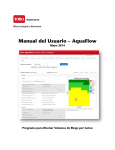
COMPUTER PROGRAM AquaFlow
AquaFlow provides designers with the information they need to design an AquaTraXX tape system for optimum performance. AquaFlow provides system operators
with the information necessary to operate the system, efficiently applying the desired
amount of water and nutrients to the crop.
AquaFlow will help you to design a complete Aqua-TraXX system, including the
selection of the Aqua-TraXX tape and the sizing of submains and mainlines. The
AquaFlow program includes both metric and U.S. measurement units in the graphic
screens for pressure profile and flow profile curves. Metric units are given in kPa
and meters. U.S. units are given in psi and feet. The following design example will
familiarize the designer with the use of the AquaFlow program.
Design Example
A designer is planning an Aqua-TraXX tape system for tomatoes. The plant rows
run downhill at a 2% slope, they are 400 feet long, and they are spaced 36 inches
apart. There will be one Aqua-TraXX line per plant row. There will be four
submains, each 100 feet long. The submains will each feed 34 tape lines, and they
will run downhill at a 1-% slope. The mainline runs parallel to the submains. The
designer has selected Aqua-TraXX tape part number EA5060867 (5/8-inch diameter,
6 mil, 8-inch spacing, 0.67 gpm/100 feet). He will run the system at an operating
pressure of 10 psi. He wants to achieve an overall EU of 90% within each submain
block.
Figure 10 below illustrates the various elements of the submain block. To begin, the
user clicks on the Red TORO icon on the computer desktop. When the Main Menu
is displayed, the user clicks on the word “Design” on the upper menu bar. Four submenu selections appear. We will use these sub-menus in sequence to complete the
design example.
Chapter V: Aqua-TraXX Design
5-3
Mainline
Submain
Riser
400’ Aqua-TraXX
Tape Laterals (34)
@ 36” O.C.
100’ Oval Hose
Submain
Flushout
Valve
Flushing
Manifold
Flushing
Valve
Figure 12: Example Submain Block.
5-4
Chapter V: Aqua-TraXX Design
Aqua-TraXX SELECTION MENU
From the AquaFlow Main Menu, click on Design, and then click on Aqua-TraXX
Selection Menu. Choose an INLET PRESSURE of 10 PSI, a LAND SLOPE of
2%, and Aqua-TraXX PART NUMBER EA5xx0867. Click the “Graph Pressure”
button.
Note: The “xx” in the part number designates the wall thickness in mils (thousandths
of an inch). Since wall thickness does not affect hydraulic design, the many wall
thicknesses available are not listed individually.
Chapter V: Aqua-TraXX Design
5-5
Aqua-TraXX SELECTION MENU: GRAPH PRESSURE
When the GRAPH PRESSURE button is clicked, AquaFlow computes and plots a
family of pressure profile curves representing tape lengths out to an EU (Emission
Uniformity) value of 80%. The pressure profile curves are color-coded to indicate
the EU value ranges for each line length. The graph below indicates that the selected
Aqua-TraXX product EA5xx0867 is suitable for run lengths as long as 550 feet at 10
psi inlet pressure and 2% slope.
5-6
Chapter V: Aqua-TraXX Design
Aqua-TraXX DESIGN MENU
With the initial selection of EA5xx0867 made, the next step is to go to the Design
Menu. AquaFlow preserves the previously entered inlet pressure, land slope, and
Aqua-TraXX part number for you. You must now enter a specific tape LENGTH
and SPACING - this is the spacing in inches from tape-to-tape across the field - and
click the GRAPH PRESSURE button. AquaFlow then computes and plots a
pressure profile curve representing the selected tape length.
Chapter V: Aqua-TraXX Design
5-7
DESIGN MENU: GRAPH PRESSURE
AquaFlow computes and plots the individual pressure profile curve representing the
tape length selected. The graph below shows the pressure profile for a 400-foot long
run, and provides design data including the inlet flow rate and the Emission
Uniformity value for the single line.
5-8
Chapter V: Aqua-TraXX Design
SUBMAIN DESIGN
Submains provide water to individual field blocks, distributing water at a uniform
pressure to the Aqua-TraXX lateral lines. Submains may be constructed of PVC
pipe, PVC layflat hose, or Oval Hose™.
Oval Hose is a popular and widely used choice for submains because it is
economical, rugged, and easy to handle and install. Oval Hose can be retrieved from
the field and used again year after year. Oval Hose is manufactured in a round
configuration, and subsequently flattened and wound on reels or in coils for ease of
handling and compact shipment. After it is installed in the field and pressurized,
Oval Hose returns to its round configuration. Aqua-TraXX tape may be connected to
Oval Hose submains using barbed connectors (FCA0798) or leader tubing.
Good submain design incorporates a flushout valve at the end of the submain, and a
flushing manifold, which is used to flush the entire block of lateral lines
simultaneously.
Submain Riser Design
A submain riser serves to regulate water flow from the mainline to the submain. A
typical submain riser assembly will normally consist of:
1.
2.
3.
4.
A screen filter to prevent debris from entering the tape lines.
A manual or pressure regulating valve to control the flow rate.
A vacuum relief valve to prevent suction in the submain and tape lines.
A Schrader valve to be used as a pressure test point.
Chapter V: Aqua-TraXX Design
5-9
SUBMAIN DESIGN MENU
With the Aqua-TraXX selection and design completed, the next step is to go to the
Submain Design Menu. As before, AquaFlow preserves the previously entered
design parameters for you. You must now select a submain material (Oval Hose or
PVC), select a pipe size, enter a submain LENGTH, SLOPE, and PRESSURE, and
click the Plot Pressure button.
Hint: To see the full list of available submain pipe selections, click on the down
arrow to the right of the Oval Hose label box.
5-10
Chapter V: Aqua-TraXX Design
SUBMAIN DESIGN MENU: PLOT PRESSURE
The Plot Pressure function plots pressure profiles of all the Aqua-TraXX lines on the
submain, superimposed on one another. These pressure profiles will vary vertically
on the graph due to the pressure variation within the submain.
Note: The submain pressure calculations begin at the downstream end of the
submain and proceed to the upstream end. Therefore, the last curve plotted is at the
submain inlet.
Chapter V: Aqua-TraXX Design
5-11
MAINLINE DESIGN
The initial stage of mainline design consists of determining its location. Laying out
the route for the mainline to follow is often a trial-and-error procedure, involving
analysis of the costs and benefits of a number of alternative routes. Once the
mainline route has been chosen, the proper pipe sizes must be specified.
For small systems the mainline can often be designed without an elevation drawing.
However, for large or complex systems it is best to prepare an elevation drawing of
the topography that the mainline will traverse. The required submain pressure in feet
is superimposed on the drawing to indicate the minimum allowable pressure at any
point. Then, the proposed hydraulic grade line may be drawn in, from the inlet of the
mainline to the end.
Once the proposed hydraulic grade line has been drawn and the required flow rates
calculated, individual sections of the mainline are sized, each section being designed
to most closely adhere to the specified hydraulic grade line. The designer must also
compute static pressures in the pipelines, and check each section to ensure that the
average water velocity does not exceed a specified limit, usually 5 to 10 feet per
second. This is done to minimize the damaging effects of waterhammer.
AquaFlow will help you to size the mainline once the maximum velocity, hydraulic
grade line and flow rates are specified. AquaFlow utilizes the Hazen-Williams
equation to compute friction losses, which is recalled here for PVC pipe (C=150) as,
Hf = 0.000977 {Q 1.852 / D 4.871} L
Where Hf
Q
D
L
=
=
=
=
Eq. 5
Friction Loss (feet of water)
Flow Rate (gpm)
Actual Pipe I.D. (inches)
Length of Pipe (feet)
Velocity of flow in a pipeline may be computed as follows,
Q/D2
V = 0.4085
Eq. 6
Where V = Velocity (ft per second)
Q = Flow Rate (gpm)
D = Actual Pipe I.D. (inches)
5-12
Chapter V: Aqua-TraXX Design
Chapter V: Aqua-TraXX Design
5-13
Mainline Design Menu
The final step in the design process is to size the mainline. For this example we will
design a mainline which feeds four of the above submain blocks simultaneously.
Click on the Mainline Design Menu. This menu will enable you to size the mainline
one segment at a time.
To start, enter the land elevations upstream and downstream, enter the downstream
flow rate (feeding the last submain) and the downstream pressure (in this case we
allow for a 5 psi pressure loss through the submain riser assembly). Select a pipe
type and click on a pipe size. Values of head loss, velocity, and upstream pressure
will appear in the appropriate boxes. You may experiment with a number of
different pipe sizes until you select the one you want: note that the Velocity box turns
yellow (warning) for velocities over 5 feet per second.
When you are satisfied, click “Next”. The program will store the design values for
the first segment and advance to the next segment, where all the steps above are
repeated. When the last segment has been completed, click “Done”.
5-14
Chapter V: Aqua-TraXX Design
Mainline Design Summary
When you click the Done box, the program displays the Mainline Design Data
summary for you on the screen as shown below.
Chapter V: Aqua-TraXX Design
5-15
5-16
Chapter V: Aqua-TraXX Design
Design Report
AquaFlow will produce a design report that can be printed out for your customer, and
will store the report on your hard drive for future reference. In order to produce the
Design Report, click Report on the main menu.
To generate the report, first verify the data presented in the Report Menu. Then
select the graphs and tables you want to include. Click the Verify Customer button
to enter or verify customer information. Click the Select Logos button to put the
Toro Ag logo, the Aqua-TraXX logo, and your company Logo on the front page of
the report. Click “Print Preview” and AquaFlow will preview the report for you on
your screen. Finally, click “Print” and AquaFlow will print the report to your printer.
Chapter V: Aqua-TraXX Design
5-17
5-18
Chapter V: Aqua-TraXX Design
CHAPTER VI
INSTALLATION PROCEDURES
INSTALLATION
The following recommendations apply to the installation of Aqua-TraXX tape:
1.
Store tape reels in a covered area, protected from sunlight and rain.
2.
Install tape with the blue stripes and outlets facing upwards. Fine soil
particles in the incoming water will normally settle to the bottom of the tape.
Installation of tape upside down may result in clogging if there is any
contamination in the incoming water.
3.
An air/vacuum relief valve should always be installed at the submain riser to
prevent suction from occurring in the tape when the system is shut down.
Suction in buried tape will tend to draw muddy water back into the tubing
through the outlets, causing contamination.
4.
Tape may be laid on the surface or buried. Burial is preferred where possible,
since it protects the tubing from accidents and animal damage, reduces
clogging, maintains tape location and alignment, reduces surface evaporation,
and insures that water is applied at the desired location.
5.
Tape must be buried when used under clear plastic mulch. Condensed water
droplets on the underside of clear plastic will focus sunlight like a magnifying
glass, burning holes in the tape.
6.
Care should be taken during installation to prevent soil, insects, and other
contaminants from getting into the tape. Ends should be closed off by
kinking or knotting until the tape can be hooked up to the system.
7.
Tape must be monitored as it is injected into the soil. Someone should be
watching to insure that the tape maintains its blue stripes upwards orientation,
to assist in case the tape becomes tangled in the injector, and to signal the
tractor driver when the tape reel is empty and must be replaced.
Chapter VI: Operation and Maintenance
6-1
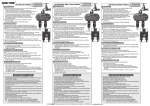
CONNECTIONS
Aqua-TraXX
tape
is
connected to Oval Hose
submains using either a
plastic fitting or a length of
leader tubing, as shown in
Fig. 10.
Fittings are
popular because they are
quickly
and
easily
installed, they provide a
strong
and
rugged
connection, and they can
be re-used for many years.
Figure 13: Aqua-TraXX Connection to Oval Hose
Figure 14: Methods of Aqua-TraXX Tape Connections
6-2
Chapter VI: Operation and Maintenance
TABLE 5: Friction Losses in PSI through Tape Connections.
Flow Rate (GPM)
1
1.5
2
2.5
3
3.5
4
FCA0798
0.23
0.49
0.83
1.25
1.74
2.31
2.95
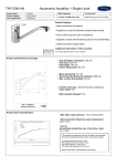
INJECTION EQUIPMENT
Figure 15: Injecting Aqua-TraXX (Casa Grande, Arizona)
Aqua-TraXX tape may be installed above or below ground with a tractor-mounted injector
tool similar to the one shown in Figure 16. This type of injector may be fabricated on the
Chapter VI: Operation and Maintenance
6-3
farm or purchased from a number of manufacturers. Typically, from two to six reels of tape
may be installed simultaneously with tractor-mounted injectors of this type.
The design of tape injection equipment should take the following into account:
1. Each tape reel should have a braking mechanism to maintain a slight tension and to
prevent reel overrunning when the tractor slows or stops. A simple and effective
braking system can be made from an 11-inch-wide strip of canvas draped over the
tape reel and fastened at one end to the injector frame. The other end of the canvas
strip is folded over and sewn, forming a pocket for weights.
2. The reels must be monitored continuously during injection to insure a quality
installation.
3. Reels are heavy – approximately 70 pounds – and procedures for mounting them
onto the tractor must take their weight into account.
4. The tractor should carry spare reels that can be mounted when a reel runs out in midfield.
5. Injection equipment used to install tape should be free of sharp edges, burrs, and
areas where the tubing could be damaged. Bends, rollers, and other points of contact
with the tape should be kept to a minimum to reduce both the possibilities for
damage and the tension on the tape as it is injected.
6-4
Chapter VI: Operation and Maintenance
E
IT
Y
T
.Q
O
N
2
1
M
3
aterilT
M
8
9
3
7
.6
1
"X
4
m
C
B
o
el.25
an
h
"C
7p
4
8
22.00
1.50
20.00
11.50
12.00
9.00
6.00
6.00
11
1.00
14.50
A
3.00
ITEM NO. QTY. M aterial
12.00
12.00
FIGURE 16: Aqua-TraXX INJECTION TOOL
Chapter VI: Operation and Maintenance
A
1
2
2
2
3" X 1.498" X .247" Channel
4" X 1.647" X .258" Channel
3
4
1
1
T ool Bar Clamp
1" X 3" Tool Steel
5
6
1
2
1 " CF Steel
3 /16" Aluminum Plate
7
1
1 1/4" Sweep Elbow
8
9
10
11
1
1
2
1
1 1/4" FPT Coupling
1 1/4" MPT Hex Bushing
1 /4" Steel Plate
1 /4" Steel Plate
6-5
6-6
Chapter VI: Operation and Maintenance
CHAPTER VII
OPERATION AND MAINTENANCE
COMPUTING IRRIGATION TIME
Once ET has been determined, the irrigation time T may be computed. In order to
perform the calculation, it is necessary to know the average Q100 flow rate (gpm per
100 feet) and the system Emission Uniformity EU.
For row crops on Aqua-TraXX tape, the irrigation time T may be computed from the
following formula:
S x ET
Q-100 x EU
T
=
1.04 x
Where T
S
ET
Q-100
EU
=
=
=
=
=
Irrigation Time (hours)
Average Tube Spacing (feet)
Evapotranspiration (inches)
Average Q100 Flow Rate (gpm per 100 feet)
System Emission Uniformity (decimal)
Eq. 7
Figure 17: Aqua-TraXX on Peppers (Florida sandy soil)
Chapter VII: Operation and Maintenance
7-1
EXAMPLE:
In a field of Pima cotton growing in Arizona, the previous day's ET value was found
to be 0.221 inches. The cotton rows are spaced 40 inches (3.33 feet) apart with
Aqua-TraXX tape buried under each row. The average flow rate is 0.30 gpm per 100
feet, and the system emission uniformity is 90 percent. Find T:
SOLUTION:
T
=
1.04 x
3.33 x 0.221
0.30 x 0.90
=
2.8 hours
On newly planted acreage, the computed ET, and therefore the irrigation time T, may
be quite low. Nevertheless, because the young plants are not likely to have extensive
root systems, it is best to apply this small amount on a frequent basis rather than
attempting to apply more water less frequently. On established crops, however, it is
usually best to have a minimum irrigation period of one hour or longer. This
minimizes uneven distribution due to mainline fill and drain times and establishes a
larger wetting pattern under each tape outlet. For example, if the irrigation time is
determined to be 35 minutes for a given day, it would probably be better to
accumulate the time for two days and irrigate 70 minutes every other day.
MONITORING SYSTEM PERFORMANCE
The well-designed micro-irrigation system will have built-in diagnostic tools that
will allow the operator to monitor the performance of the system, and to detect
possible problems in the early stages. Included in this category are flow meters,
pressure gauges, and submain riser filters.
Flow Meters
System flow meters should be installed on the main supply lines, and should provide
readings of both instantaneous and cumulative flow. These meters should be read
regularly and the readings kept in a logbook. Variations in the system flow rate may
indicate that something in the system is amiss.
For example, a gradual decline in system flow rate as measured by the flow meters
may indicate a problem with the pumping station or a clogging problem in the field.
On the other hand, an unexpected increase in the system flow rate might be an
indication of a pipeline break or the presence of leakage in the system.
Measurements of cumulative flow will serve to verify water application schedules.
7-2
Chapter VII: Operation and Maintenance
Pressure Test Points
The system should have sufficient pressure testing points so that an overall check of
the system pressures can be made. Widely differing pressures in different sections of
the system may indicate that some blockage, leakage, or other problem has arisen in
some section of the system. Pressure checks should be regularly made, and the
pressures recorded.
Submain Riser Filters
Submain riser filters are small, in-line or “wye” strainers installed at each submain
riser. Under normal conditions these filters, which are usually 80 - 120 mesh, will
collect few if any contaminants because the main filtration system will normally have
removed this material. Periodic examination of these riser filters can be a valuable
indication that the system is contaminated. In the case of a pipeline break or a failure
of the main filter station, riser filters will help to prevent foreign material from
entering the tape lines.
MAINTENANCE PROCEDURES FOR Aqua-TraXX TAPE
Flushing
In many micro-irrigation systems it has been found that provisions must be made to
flush submain lines and lateral lines to remove settled sediments, and flushing
constitutes an important maintenance routine. Research has shown that most settled
sediments can be flushed from pipe or tubing with a flow velocity of one foot per
second, which is referred to as the "scour velocity". In standard half-inch lateral
lines, the 1 ft/sec scour velocity is equivalent to a flow rate of 1 gpm at the
downstream end.
Mainlines, submains and lateral lines should be flushed thoroughly prior to system
startup, and tape lines should be regularly flushed during the season. Open the ends
of the lateral lines while the system is running and allow water to run into a container
until it runs clear. Collect some of the dirty water in a glass jar, and examine it
carefully. Take note of the nature of the impurities in the water. If there is a
significant amount of contaminant in the flush water, find out what it is. Does it
appear to be a bacterial slime? Are large aggregated particles present? Is there
evidence of iron precipitation? Is there any material which could be sand from the
media filter?
Examine the contaminant under a microscope. Put samples of the dirty water into
two small jars or test tubes. Treat one with a few drops of chlorine bleach and the
Chapter VII: Operation and Maintenance
7-3
other with a few drops of hydrochloric acid. Note any changes: chlorine will attack
organic matter, while acid will dissolve many inorganic precipitates. Acid or
chlorine will not affect soil and sand particles.
Prevention of Clogging
The biggest potential problem facing the operator of a micro-irrigation system is
clogging. Because the water passages in most tape emitters are very small, they
easily become clogged by particles of mineral or organic matter. This can reduce
emission rates, cause non-uniformity of water distribution, and thereby cause stress
and damage to the crop.
Growers sometimes inadvertently cause clogging by injecting inappropriate
chemicals or other substances into their systems.
In some cases, contaminants are present in irrigation water delivered to the user and
are not adequately filtered out. These contaminants may include soil particles, living
or dead organic materials, and scale from rusty pipes. In other cases, contaminants
enter the system during the installation phase, and are not adequately flushed out of
the system. Included in this category are insects, Teflon tape, PVC pipe shavings,
and soil particles. Pipeline breaks often result in system contamination with soil,
causing subsequent clogging problems.
In buried systems, soil particles may enter, or be sucked into, tape outlets. Roots
may grow into these buried outlets to plug them.
Finally, contaminants may grow, aggregate, or precipitate in water as it stands in the
lines or evaporates from tape outlets between irrigations. Iron oxide, manganese
dioxide, calcium carbonate, algae, and bacterial slimes can form in micro-irrigation
systems under certain circumstances.
The solution to a particular clogging problem must be based upon the nature of the
problem. Acid treatment has been used successfully to dissolve calcium precipitates,
and chlorine is frequently used to decompose organic materials.
Once a system is badly clogged, there is usually little that can be done to fix it.
Therefore, the wisest course is to prevent clogging in the first place. Experience has
shown that most clogging problems can be avoided by following a few simple rules:
1.
Analyze the source water for suspended and dissolved solids, and design the
irrigation, chemical injection, and filter systems accordingly.
2. Install secondary filters on submain risers to protect the system from pipeline
breaks or filter system failures.
7-4
Chapter VII: Operation and Maintenance
3. Install vacuum breakers on submain risers to prevent suction in lateral lines.
4. Take care during installation to minimize contamination by soil, insects, pipe dope,
PVC pipe shavings, and the like.
5. Thoroughly flush the system before connecting tape to submains.
6. Practice regular chemical treatment (acid or chlorine).
7. Flush tape lines on a regular basis.
Prevention of Insect Damage
Ants, wireworms, and other insects may cause damage to tape. Insect damage typically
takes the form of holes chewed through the sides of tape. Researchers have noted that insect
damage is most severe in tape having wall thicknesses of less than 10 mils (0.010 inches).
Insect damage has been successfully controlled with insecticides. However, these chemicals
are highly toxic and persist in the environment. For this reason, growers are advised to
select a tape with sufficient wall thickness to prevent insects from making holes through the
wall of the tubing.
Prevention of Root Intrusion
In micro-irrigation systems utilizing buried tape, plant roots may grow into tape outlets,
effectively clogging them. This so-called “root intrusion” into tape outlets may be
widespread throughout the field, severely compromising the effectiveness of the irrigation
system. In advanced cases, there is no alternative but to replace the tape.
The tendency for root intrusion to occur varies widely according to crop type, the type of
system components selected, depth and placement of the drip tape, and irrigation scheduling
practices. It is known that moisture stress encourages plant root structures to expand more
aggressively, seeking water. It is also known that roots will find and follow a seam on
buried drip tape, and grow into outlets if they are placed along this seam.
Two of the most effective preventive measures against root intrusion are to schedule
irrigation in such a way as to avoid moisture stress, and to select tape types which do not
have a seam. Drip tapes employing slit type outlets are considerably less susceptible to root
intrusion than are those with hole type outlets.
Other measures employed against root intrusion are chemical treatments with acid,
acidic fertilizers, chlorine, or chemicals, which retard root growth. It must be noted that this
type of chemical treatment, because it is used to retard the roots of the crop, may lead to
Chapter VII: Operation and Maintenance
7-5
serious crop damage if done incorrectly. Growers are strongly encouraged to seek expert
advice before attempting chemical treatments to discourage root intrusion.
7-6
Chapter VII: Operation and Maintenance
Chapter VII: Operation and Maintenance
7-7
APPENDIX A
CONVERSION FACTORS
TO CONVERT
acres
acres
INTO
hectares
sq feet
MULTIPLY BY
0.4047
43,560
acres
sq meters
acres
sq miles
4,047
acres
sq yards
4,840
acre-feet
cu feet
43,560
acre-feet
gallons
3.259x10+5
atmospheres
ft of water
33.90
atmospheres
in of mercury
29.92
atmospheres
kg/sq cm
1.0333
atmospheres
kg/sq meter
10,332
atmospheres
pounds/sq in
14.70
bars
atmospheres
0.9869
bars
dynes/sq cm
1.0x10+6
bars
kg/sq meter
1.020x10+4
bars
pounds/sq ft
2,089
bars
pounds/sq in
14.50
BTU
kilowatt-hrs
2.928x10-4
Centigrade
Fahrenheit
(C x 1.8)+32
centimeters
feet
3.281x10-2
centimeters
inches
centimeters
millimeters
10
cubic centimeters
cu inches
0.06102
1.562x10-3
0.3937
cubic centimeters
gallons (U.S.)
cubic centimeters
liters
2.642x10-4
cubic centimeters
pints (U.S.)
2.113x10-3
cubic centimeters
quarts (U.S.)
1.057x10-3
cubic feet
cu cm
cubic feet
cu inches
1,728
cubic feet
cu meters
0.02832
cubic feet
cu yards
0.03704
cubic feet
gallons (U.S.)
7.48052
cubic feet
liters
28.32
cubic feet
pints (U.S.)
59.84
cubic feet
quarts (U.S.)
29.92
0.001
28,320
cubic feet/sec
million gals/day
0.646317
cubic feet/sec
gallons/min
448.831
cubic inches
cu cm
16.39
cubic inches
gallons
4.329x10-3
cubic inches
liters
cubic meters
cu yards
1.308
cubic meters
gallons (U.S.)
264.2
cubic meters
liters
1,000
TO CONVERT
Toro Micro-Irrigation Design Manual
0.01639
INTO
MULTIPLY BY
A-1
Dynes/sq cm
Dynes/sq cm
atmospheres
in of mercury at 0° C
9.869x10-7
2.953x10-5
Dynes/sq cm
in of water at 4° C
4.015x10-4
Dynes/sq cm
bars
feet
centimeters
30.48
feet
kilometers
3.048x10-4
feet
meters
0.3048
feet of water
atmospheres
0.02950
feet of water
in of mercury
0.8826
feet of water
kg/sq meter
304.8
feet of water
pounds/sq in
0.4335
gallons
cu cm
3,785
gallons
cu feet
0.1337
gallons
cu inches
231
gallons
cu meters
3.785x10-3
gallons
cu yards
4.951x10-3
gallons
liters
gallons (Imp.)
gallons (U.S.)
1.20095
gallons (U.S.)
gallons (Imp.)
0.83267
gallons of water
pounds of water
gallons/min
cu ft/sec
2.228x10-3
gallons/min
liters/sec
0.06308
gallons/min
cu ft/hr
8.0208
hectares
acres
2.471
hectares
sq feet
1.076x10+5
horsepower
Btu/min
42.44
horsepower
foot-lbs./min
33,000
horsepower
foot-lbs./sec
horsepower (metric)
horsepower (British)
0.9863
horsepower (British)
horsepower (metric)
1.014
horsepower
kg-calories/min
10.68
horsepower
kilowatts
0.7457
horsepower
watts
745.7
inches
centimeters
inches
meters
2.54x10-2
inches
miles
1.578x10-5
inches
millimeters
25.4
inches
mils
1,000
inches
yards
in of mercury
atmospheres
in of mercury
feet of water
in of mercury
kg/sq cm
in of mercury
kg/sq meter
3.785
8.3453
550
2.54
2.778x10-2
0.03342
1.133
0.03453
345.3
in of mercury
pounds/sq ft
70.73
in of mercury
pounds/sq in
0.4912
in of water
atmospheres
2.458x10-3
in of water
inches of mercury
in of water
kg/sq cm
in of water
ounces/sq in
TO CONVERT
in of water
A-2
1.0x10-4
0.07355
2.540x10-3
INTO
pounds/sq ft
0.5781
MULTIPLY BY
5.204
Toro Micro-Irrigation Design Manual
in of water
kilograms
pounds/sq in
pounds
0.03613
2.205
kilograms/cu meter
pounds/cu ft
0.06243
kilograms/hectare
pounds/acre
0.8924
kilograms/sq cm
dynes
980,665
kilograms/sq cm
atmospheres
0.9678
kilograms/sq cm
feet of water
32.81
kilograms/sq cm
in of mercury
28.96
kilograms/sq cm
pounds/sq ft
2,048
kilograms/sq cm
pounds/sq in
14.22
kilograms/sq meter
atmospheres
9.678x10-5
kilograms/sq meter
bars
98.07x10-6
kilograms/sq meter
ft of water
3.281x10-3
kilograms/sq meter
in of mercury
2.896x10-3
kilograms/sq meter
pounds/sq ft
0.2048
kilograms/sq meter
pounds/sq in
1.422x10-3
kilometers
feet
3,281
kilometers
meters
1,000
kilometers
miles
0.6214
kilometers
yards
1,094
kilometers/hr
feet/min
54.68
kilometers/hr
feet/sec
0.9113
kiloPascals (kPa)
pounds/sq in
0.14503
kilowatts
BTU/min
56.92
kilowatts
horsepower
1.341
kilowatt-hrs
BTU
3,413
kilowatt-hrs
horsepower-hrs
1.341
liters
cu cm
1,000
liters
cu feet
0.03501
liters
cu inches
61.02
liters
cu meters
liters
cu yards
0.001
liters
gallons (U.S.)
0.2642
liters
pints (U.S.)
2.113
liters
quarts (U.S.)
1.057
liters/min
cu ft/sec
5.886x10-4
liters/min
gals/sec
4.403x10-3
liters/sec
gallons/min
15.852
liters/sec-sq meter
gallons/min-sq ft
1.4726
meters
centimeters
meters
feet
1.308x10-3
100
3.281
meters
inches
39.37
meters
kilometers
0.001
meters
miles (naut.)
5.396x10+4
meters
miles (stat.)
6.214x10+4
meters
millimeters
1,000
meters
yards
1.094
meters/min
miles/hr
0.03728
meters/sec
feet/min
196.8
TO CONVERT
INTO
meters/sec
feet/sec
meters/sec
kilometers/hr
Toro Micro-Irrigation Design Manual
MULTIPLY BY
3.281
3.6
A-3
A-4
meters/sec
meters/sec
kilometers/min
miles/hr
0.06
2.237
meters/sec
miles/min
miles (statute)
feet
miles (statute)
inches
miles (statute)
kilometers
miles (statute)
meters
1,609
miles/hr
cm/sec
44.70
miles/hr
feet/min
88
miles/hr
feet/sec
1.467
milligrams/liter
parts/million
milliliters
liters
0.03728
5,280
6.336x10+4
1.609
1
0.001
millimeters
centimeters
millimeters
inches
millimeters
mils
million gals/day
cu ft/sec
0.1
0.03937
39.37
1.54723
mils
centimeters
mils
inches
2.540x10-3
parts/million
pounds/million gal
pounds
dynes
44.4823x10+4
pounds
grams
453.5924
pounds
kilograms
pounds
ounces
16
pounds of water
gallons
0.1198
pounds/cu ft
grams/cu cm
0.01602
pounds/cu ft
kg/cu meter
16.02
pounds/sq in
atmospheres
0.06804
pounds/sq in
bars
0.0689
pounds/sq in
ft of water
2.307
pounds/sq in
in of mercury
2.036
pounds/sq in
kPa
6.895
pounds/sq in
kg/sq meter
703.1
pounds/sq in
pounds/sq ft
quarts (liq.)
liters
0.9463
square miles
acres
640
square meters
square feet
square meters
square inches
tonnes (metric)
kilograms
1,000
tonnes (metric)
pounds
2,205
0.001
8.345
0.4536
144
10.7639
1,550
tons (short)
kilograms
tons (short)
pounds
907.1848
2,000
tons (short)
tonnes (metric)
0.9078
yards
meters
0.9144
Toro Micro-Irrigation Design Manual
APPENDIX B
REFERENCE TABLES OF SELECTED DATA
TABLE B-1: ROUGHNESS COEFFICIENT C VALUES FOR HAZEN-WILLIAMS EQUATION
VALUES OF C
TYPE OF PIPE
PVC
Polyethylene
Asbestos-Cement
Cement-Lined Steel
Welded Steel
Riveted Steel
Concrete
Cast Iron
Copper, Brass
Wood Stave
Vitrified Clay
Corrugated Steel
RANGE
160 - 145
150 - 130
160 - 140
160 - 140
150 - 80
140 - 90
150 - 85
150 - 80
150 - 120
145 - 110
NEW PIPE
150
140
150
150
140
110
120
130
140
120
110
60
DESIGN C
150
140
140
140
100
100
100
100
130
110
100
60
Above values of C for use with Hazen-Williams Equation, friction head losses in feet per
foot of pipe length for fresh water at 50 degrees Fahrenheit.
Hf =
Where Hf
C
Q
L
D
=
=
=
=
=
10.472
x
C1.852
Q1.852
D4.871
xL
Friction Head Loss (ft)
Roughness Coefficient
Flow Rate (gpm)
Pipe Length (ft)
Pipe Inner Diameter (inches)
Toro Micro-Irrigation Design Manual
B-1
TABLE B-2: FRICTION LOSS IN POLYETHYLENE (PE) SDR RATED TUBE
LOSSES IN PSI PER 100 FEET OF TUBE (PSI/100 FT) C = 140
SIZE ID GPM
0.50
(0.622)
0.75
(0.824)
1.00
(1.049)
1.25
(1.380)
1.50
(1.610)
2.00
(2.067)
1
2
3
4
5
6
7
8
9
10
12
14
16
18
20
22
24
26
28
30
35
40
45
50
55
60
65
70
75
80
85
90
95
100
110
120
130
140
150
160
170
180
190
200
225
250
275
300
325
350
375
400
425
450
475
500
550
600
0.49
1.76
3.73
6.35
9.60
13.46
0.12
0.45
0.95
1.62
2.44
3.43
4.56
5.84
7.26
8.82
12.37
0.04
0.14
0.29
0.50
0.76
1.06
1.41
1.80
2.24
2.73
3.82
5.08
6.51
8.10
9.84
11.74
13.79
16.00
18.35
0.01
0.04
0.08
0.13
0.20
0.28
0.37
0.47
0.59
0.72
1.01
1.34
1.71
2.13
2.59
3.09
3.63
4.21
4.83
5.49
7.31
9.36
11.64
14.14
16.87
0.00
0.02
0.04
0.06
0.09
0.13
0.18
0.22
0.28
0.34
0.48
0.63
0.81
1.01
1.22
1.46
1.72
1.99
2.28
2.59
3.45
4.42
5.50
6.68
7.97
9.36
10.86
12.46
14.16
15.95
17.85
0.00
0.01
0.01
0.02
0.03
0.04
0.05
0.07
0.08
0.10
0.14
0.19
0.24
0.30
0.36
0.43
0.51
0.59
0.68
0.77
1.02
1.31
1.63
1.98
2.36
2.78
3.22
3.69
4.20
4.73
5.29
5.88
6.50
7.15
8.53
10.02
11.62
13.33
15.15
17.08
B-2
2.50
(2.469)
0.06
0.08
0.10
0.13
0.15
0.18
0.21
0.25
0.29
0.32
0.43
0.55
0.69
0.83
1.00
1.17
1.36
1.56
1.77
1.99
2.23
2.48
2.74
3.01
3.59
4.22
4.90
5.62
6.38
7.19
8.05
8.95
9.89
10.87
13.52
16.44
19.61
3.00
(3.068)
0.05
0.07
0.09
0.10
0.11
0.15
0.19
0.24
0.29
0.35
0.41
0.47
0.54
0.61
0.69
0.77
0.86
0.95
1.05
1.25
1.47
1.70
1.95
2.22
2.50
2.80
3.11
3.44
3.78
4.70
5.71
6.82
8.01
9.29
10.65
12.10
13.64
15.26
16.97
4.00
(4.026)
0.08
0.09
0.11
0.13
0.14
0.16
0.18
0.21
0.23
0.25
0.28
0.33
0.39
0.45
0.52
0.59
0.67
0.75
0.83
0.92
1.01
1.25
1.52
1.82
2.13
2.48
2.84
3.23
3.64
4.07
4.52
5.00
5.50
6.56
7.70
6.00
(6.065)
0.03
0.03
0.03
0.03
0.04
0.05
0.05
0.06
0.07
0.08
0.09
0.10
0.11
0.12
0.14
0.17
0.21
0.25
0.29
0.34
0.39
0.44
0.50
0.55
0.62
0.68
0.75
0.89
1.05
Toro Micro-Irrigation Design Manual
TABLE B-3: FRICTION LOSS TABLES FOR LAYFLAT HOSE
LOSSES IN PSI PER 100 FEET OF TUBE (PSI/100 FT) C = 140
SIZE ID
GPM
0.50
0.63
0.75
1.00
1.25
1.50
1
2
3
4
5
6
7
8
9
10
11
12
13
14
15
16
17
18
19
20
22
24
26
28
30
32
34
36
38
40
42
44
46
48
50
52
54
56
58
60
62
64
66
68
70
75
80
85
90
95
100
105
110
115
120
125
130
135
140
145
150
160
170
1.41
5.09
10.77
18.34
0.48
1.72
3.64
6.19
9.36
13.11
17.44
0.20
0.71
1.50
2.55
3.85
5.40
7.18
9.19
11.43
13.89
16.57
19.47
0.05
0.18
0.37
0.63
0.95
1.33
1.77
2.27
2.82
3.43
4.09
4.80
5.57
6.39
7.26
8.18
9.15
10.15
11.24
12.35
14.74
17.31
0.02
0.06
0.13
0.21
0.32
0.45
0.60
0.77
0.95
1.16
1.38
1.62
1.88
2.16
2.45
2.76
3.09
3.43
3.79
4.17
4.98
5.85
6.78
7.77
8.83
9.95
11.13
12.38
13.68
15.04
16.46
17.94
19.48
0.01
0.02
0.05
0.09
0.13
0.19
0.15
0.32
0.39
0.48
0.57
0.67
0.77
0.89
1.01
1.14
1.27
1.41
1.56
1.72
2.05
2.41
2.79
3.20
3.64
4.10
4.59
5.10
5.63
6.19
6.78
7.39
8.02
8.68
9.36
10.06
10.79
11.54
12.32
13.11
13.93
14.78
15.64
16.53
17.44
19.82
SIZE ID GPM
2.00
0.08
0.10
0.12
0.14
0.17
0.19
0.22
0.25
0.28
0.31
0.35
0.39
0.42
0.51
0.59
0.69
0.79
0.90
1.01
1.13
1.26
1.39
1.53
1.67
1.82
1.98
2.14
2.31
2.48
2.66
2.85
3.04
3.23
3.44
3.65
3.86
4.08
4.30
4.89
5.51
6.16
6.85
7.57
8.32
9.11
9.93
10.78
11.66
12.58
13.52
14.50
15.51
16.55
2.00
2.50
0.14
0.17
0.20
0.23
0.27
0.30
0.34
0.38
0.43
0.47
0.52
0.57
0.62
0.67
0.72
0.78
0.84
0.90
0.96
1.03
1.09
1.16
1.23
1.30
1.38
1.45
1.65
1.86
2.08
2.31
2.56
2.81
3.08
3.35
3.64
3.94
4.25
4.57
4.90
5.24
5.59
5.95
6.70
7.50
0.21
0.23
0.25
0.28
0.30
0.32
0.35
0.37
0.40
0.42
0.45
0.48
0.51
0.54
0.57
0.60
0.68
0.77
0.86
0.95
1.05
1.16
1.27
1.38
1.50
1.62
1.75
1.88
2.02
2.16
2.30
2.45
2.76
3.09
0.11
0.12
0.13
0.13
0.14
0.15
0.17
0.19
0.21
0.24
0.26
0.29
0.31
0.34
0.37
0.40
0.43
0.46
0.50
0.53
0.57
0.60
0.68
0.76
0.04
0.05
0.05
0.06
0.06
0.07
0.07
0.07
0.08
0.08
0.10
0.11
2.50
3.00
4.00
6.00
Toro Micro-Irrigation Design Manual
3.00
4.00
6.00
8.00
B-3
180
190
200
210
220
230
240
250
260
270
280
290
300
325
350
375
400
425
450
475
500
550
600
650
700
800
900
1,000
1,100
1,200
1,300
1,400
1,500
2,000
2,500
B-4
8.34
9.21
10.13
11.09
12.08
13.12
3.43
3.79
4.17
4.57
4.98
5.40
5.85
6.30
6.78
7.27
7.78
8.30
8.83
10.24
0.85
0.94
1.03
1.13
1.23
1.33
1.44
1.56
1.67
1.79
1.92
2.05
2.18
2.53
2.90
3.29
3.71
4.15
4.61
5.10
5.61
6.69
0.12
0.13
0.14
0.16
0.17
0.19
0.20
0.22
0.23
0.25
0.27
0.29
0.30
0.35
0.40
0.46
0.52
0.58
0.64
0.71
0.78
0.93
1.09
1.27
1.45
1.86
2.31
2.81
3.35
3.94
4.57
0.03
0.04
0.04
0.05
0.05
0.05
0.06
0.06
0.07
0.07
0.08
0.09
0.10
0.11
0.13
0.14
0.16
0.18
0.19
0.23
0.27
0.31
0.36
0.46
0.57
0.69
0.83
0.97
1.13
1.29
1.47
2.50
3.78
Toro Micro-Irrigation Design Manual