1
AquaFlow user manual
Irrigation design software
1
TABLE OF CONTENTS
CHAPTER 1:
Getting started
AquaFlow design software
Installing AquaFlow
Literature files
Program files
CHAPTER 2: Beginning the design
Main Menu
Parts Database
Entering customer information
Selecting a customer
Design Example
CHAPTER 3:
Custom parts inputs
Database selection
CHAPTER 4:
Emission Uniformity (EU)
Application Efficiency (EA)
APPENDIX: Roughness Coefficient, C Values for Hazen-Williams Equation
2
Chapter 1
AquaFlow Design Software:
AquaFlow provides designers with the information they need to design a micro-irrigation
system for optimum performance. AquaFlow provides system operators with the
information necessary to operate the system, efficiently applying the desired amount of
water and nutrients to the crop.
AquaFlow will help you to design a complete micro-irrigation system, including the
selection of the laterals and the sizing of submains and mainlines. The AquaFlow
program includes both metric and U.S. measurement units in the graphic screens for
pressure profile and flow profile curves. Metric units are given in kPa and meters. U.S.
units are given in psi and feet. The following text will familiarize the designer with the
use of the AquaFlow program.
Installing AquaFlow onto a computer:
AquaFlow install disk
Insert the AquaFlow disk, shown above, into your CD Rom drive, the disk will
execute automatically. The disk also has Toro Ag literature cut sheets in PDF file
format (Acrobat Reader is required to view literature files and can be downloaded
at no cost at: http://www.adobe.com/products/acrobat/readstep.html). If you need a
copy of the AquaFlow installation disk or an upgrade to the most current version,
contact the following:
Toro Ag Irrigation
1588 North Marshall Ave.
El Cajon, Ca 92020
Telephone: 619-562-2950
Facsimally: 619-258-9973
Customer service: 800-333-8125
Web site: www.toroag.com
3
After inserting the AquaFlow disk in the cd rom drive the following screen appears:
Click on the link AquaFlow Design Program to install the software to the hard drive.
Click on the link: Literature to access the Toro Ag literature in PDF file format; click on
the link: AquaFlow Design Program to install the AqauFlow design software to the hard
drive; click on the link: Contacts to access contact information.
After clicking on AquaFlow Design Program, follow the instructions and the install
wizard will create folders in the program directory: C:\Program Files\Toro.
In addition, a shortcut icon will be placed on the desk top. Double click on the desktop
icon and the program will open.
4
Chapter 2
Starting the design:
Double click on the AquaFlow icon located on the desk top to open the program; the
following screen will appear:
You are now in the Main Menu. AquaFlow uses a database to store all the information
used by the program in calculating pressure and flow variation in a system. The database
has the following Toro Ag products lines stored in the lateral selection menu:
Aqua Traxx
Aqua-Traxx PC
Drip In Classic
Drip In Mining Classic
Drip In PC
Dura-Traxx
Mine-Traxx
NGE emitters
Custom parts
5
Note: Custom parts inputs are available in the lateral selection menu. (See Chapter 3)
The database also contains Oval hose, Lay Flat and PVC for designing submains and
mainlines. Custom part inputs are also available in both the Submain selection menu and
the Mainline selection menu. (See Chapter 3)
To view the database, in the main menu, go to view, then select Parts Database. The
parts database window will open.
Click to
expand
product line.
6
The parts database can be expanded by clicking on the square box with the + sign in it
located to the left of the Product line. This will allow the user to view the product
specifications used by the program to calculate the hydraulic data.
When finished viewing the database click on the Close Button to return to the Main
Menu.
Entering customer information:
The AquaFlow program will create a database of customers and designs that will be
stored in the reports folder located on the hard drive:
C:\Program Files\Toro\AquaFlow\Reports
To enter customer information, in the Main Menu select, file, Add customer.
7
The Toro Customer information window will open:
Dropdown box
will list customers
that have been
previously entered.
Design Example
A designer is planning an Aqua-Traxx tape system for tomatoes. The plant rows run
downhill at a 1.1% slope, they are 400 feet long, and they are spaced 60 inches apart.
There will be one Aqua-Traxx line per plant row. There will be four submains, each 200
feet long. The submains will each feed 41 tape lines, and they will run downhill at a
slope of 1%. The mainline runs parallel to the submains. The designer has selected
Aqua-Traxx tape part number EA5080867 (5/8-inch diameter, 8 mil, 8-inch spacing, 0.67
gpm/100 feet). He will run the system at a lateral inlet pressure of 12 psi. He wants to
achieve an overall Emission Uniformity (EU) of 90% or greater within each submain
block. A flushing velocity of 1.1 feet per second is required flushing one lateral at a time
with the end pressure of the lateral during the flushing event set a 1 psi.
If starting a design for a customer that has been previously entered, click on the
dropdown box and select the customer from the database. If starting a design for a new
customer, select the New button and enter the information in each field, all fields are
required. Once the information is entered click on OK, this will return you to the Main
Menu.
The next step in the design is to select a customer for whom the design is for. In the
Main Menu, go to System Design, Select Customer.
8
The Toro Customer information window will open; use the dropdown box to select the
customer that the design is for. By clicking on the New button, information for a new
customer may also be inputted. Once a customer is selected, click on the OK button, this
will return you to the Main Menu.
You are now ready to select a lateral. In the Main Menu, select System Design, Lateral
selection.
The Lateral selection Menu window will open:
Dropdown box with a
list of Toro Ag product
lines that can be selected
as a lateral.
Use the dropdown box under PRODUCT LINE to select the product line you wish to use
as a lateral.
The dropdown box will list a number of product lines to choose from.
9
List of Toro Ag
Product lines to
choose from
Next, select a product line; for this example Aqua-Traxx drip tape will be selected.
Spinner buttons
used to enter
land slop and
inlet pressure.
Scroll bar
Next, use the up and down scroll bar to scroll through the list of part with different flow
rates and spacing that Aqua-Traxx is available in. In this example, Aqua-Traxx 5/8
diameter, eight inch spacing with a flow rate of 0.67 gpm per 100 feet is selected.
Note: The xx in the part number denotes wall thinness in mils (1 mil = 1/1000 of an
inch). Since the mil thickness does not affect the hydraulic computations, the many
different wall thicknesses are not listed. The mil thickness will affect the operating
pressure range. Check specifications for operating pressure range for each product.
Next, use the spinner buttons to input the land slope and inlet pressure. Land slope must
be entered in % slope in increments of 0.1%, positive (+) is for downhill and negative (-)
is for uphill. In this example 1.1% downhill slope and an inlet pressure of 12 psi is
selected.
10
After the part number for the lateral is selected and the land slope and inlet pressure
inputted, next, click on the Graph Pressure button.
The Toro Ag performance curves window will now open.
AquaFlow computes and plots a family of pressure profile curves representing lateral
lengths out to an EU value of 85% or until the minimum operating pressure is exceeded.
The pressure profile curves are color coded to indicate the EU value ranges for each
11
lateral length. The graph on the previous page indicates that the selected Aqua-Traxx
product EA5xx0867 is suitable for run lengths as long as 500 feet at a 12 psi inlet
pressure and 1.1% slope. Click OK to return to the lateral selection menu.
Next, click on the Go To Design button, the following window will open:
Next, click in the window under LENGTH (FT) and enter the lateral length in feet; in this
example the lateral is 400 feet long. Next, enter the row spacing in inches; in this
example the row spacing is 60 inches. The AquaFlow program also has the ability to
12
calculate flushing velocities in feet per second at the end of the lateral and both inlet and
outlet flow rates in gpm during the flushing event. If flushing information is not required
the program default is to proceed to the next window without calculating flushing data.
In this example a minimum flushing velocity of 1.1 feet per second is required with a
lateral end pressure of 1 psi. The designer now has two choices in calculating flushing
velocity: First, by selecting the Inlet Pressure option-button, AquaFlow will calculate
the inlet pressure required to attain an inputted flushing velocity given an inputted lateral
end pressure. Second, by selecting the Flushing Vel (Flushing Velocity) option button,
AquaFlow will calculate the flushing velocity given an inputted inlet pressure and an
inputted lateral end pressure. In this example both calculations will be performed for
demonstration purposes.
First, select the Inlet Pressure option-button to calculate the minimum inlet pressure to
attain the desired flushing velocity. In this example a minimum flushing velocity of 1.1
feet per second is entered in the flushing velocity field. In the End PSI field, 1 psi is
entered. In any subsurface system it is recommended that a 1 psi end pressure be
assumed to account for elevation and soil compaction even if the ends are to be opened to
atmosphere.
Next, click on the Calculate button and AquaFlow will calculate the flushing velocities
and present the data before continuing to the next window. This provides the designer an
opportunity to adjust the inputs if the results are not satisfactory.
13
Flushing Calculation
Results window
The Flushing Calculation Results window will open providing the following information:
Inlet Flow: The demand of a single lateral in gpm during the flushing event.
Outlet Flow: The amount of flushing water in gpm exiting a single lateral during the
flushing event.
Inlet Pressure: The inlet pressure in psi required during the flushing event.
End Pressure: The pressure at the end of the lateral during the flushing event.
Flushing Velocity: This is the velocity of the water exiting the lateral in feet per second.
Flushing Travel Time: This is the time it takes a molecule of water to travel from the
inlet of the lateral to the end of the lateral during the flushing event.
Next, click on the OK button to return to the previous screen. If the flushing calculations
are unsatisfactory, the designer has the option of reentering new values in the flushing
screen until acceptable results are found.
For demonstration purposes the flushing velocities will be recalculated, this time the
Flushing Vel option button will be selected. The inlet pressure will be 12 psi and the
lateral end pressure will be 1 psi.
14
Click on the Calculate button to view the results. In this example, by raising the inlet
pressure to 12 psi during the flushing event, the flushing velocity goes from 1.1 feet per
second to 2.08 feet per second. In an actual flushing event, an end user will most likely
open up multiple laterals to flush at one time which may cause the submain pressure to
drop. In this example as long as the lowest pressure in the subamin does not drop below
3.64 psi the flushing velocity will not drop below the minimum flushing velocity of 1.1
feet per second required in this example.
Note: As a general rule, flushing velocities of 1 foot per second or higher are
recommended in order to ensure adequate lateral flushing.
If acceptable values are not possible with the lateral selected the designer may have to
return to the selection menu and select a new part for the lateral. If the designer is
satisfied with the flushing results, the next step would be to proceed to the next window
by clicking on the GRAPH PRESSURE button.
DESIGN MENU: GRAPH PRESSURE
AquaFlow computes and plots the individual pressure profile curve representing the
lateral length selected. The graph on the next page shows the pressure profile for a 400foot long lateral, and provides design data including the inlet flow-rate, Emission
Uniformity (EU) and Application Efficiency (EA) values for the single lateral. Chemical
travel time, the time it takes a molecule of water to travel from the inlet of the lateral to
15
the last emitter during the irrigation event is also included.
provided.
Flushing data is also
Drop down box can be used to adjust the scale of the graph to accommodate higher
pressures and/or longer length of run.
SUBMAIN DESIGN
Submains provide water to individual field blocks, distributing water at a uniform
pressure to the Aqua-Traxx lateral lines. Submains may be constructed of PVC pipe,
PVC Lay-Flat hose, or Oval Hose™.
SUBMAIN DESIGN MENU
With the lateral selected and design completed, the next step is to go to the Submain
Design Menu. As before, AquaFlow preserves the previously entered design parameters
for you. You must now select a submain material Oval Hose, Lay Flat or PVC.
16
Dropdown box with
different pipe materials
Next, select a pipe size from a database by using the scroll bar as shown below:
Note: Custom submain pipe inputs are also available (See Chapter 3).
Scroll bar used to view
different pipe sizes
Next, enter a submain length in feet, select the Option button for an Up or down hill
sloping submain, use the spinner buttons to enter the % slope. Next, enter the pressure;
this will be the pressure at the end of the submain. Once all the inputs are made, click the
Plot Pressure button.
In this example, a submain block is 200 feet long and is on a 1.0% downhill slope from
the inlet to the submain.
17
SUBMAIN DESIGN MENU: PLOT PRESSURE
The Plot Pressure function plots pressure profiles of all the lateral lines on the submain,
superimposed on one another. These pressure profiles will vary vertically on the graph
due to the pressure variation within the submain.
Note: The submain pressure calculations begin at the downstream end of the submain
and proceed to the upstream end. Therefore, the last curve plotted is at the submain inlet.
AquaFlow will graph the pressure profile of the submain, block Emission Uniformities
(EU) of greater than 90% will be graphed in green, EU’s of 85% to 89% will be graphed
in blue and a block EU of less than 85% will be graphed in red. It is recommended that
system EU be designed at 90% or better. In the bottom right corner of the graph the
following data is presented:
•
•
•
•
•
•
•
The number of lateral on the submain
Submain material and pipe size
Length of the submain in feet
Submain flow rate in gpm
Submain inlet pressure required
Submain end pressure
Pressure variation in the submain (not the entire block)
18
•
•
•
Emission Uniformity of the entire submain block
Chemical travel time of the last row of the submain from the inlet
Chemical travel time of the entire block
Note: The Block chemical travel time is the amount of time in minutes it takes for a
molecule of water to travel from the inlet of the submain to the exit of the last emitter of
the last lateral.
Next, click on OK
This will bring you back to the previous screen:
Click on the Go To Mainlines button, the mainline design window will open:
19
Mainline Design Menu
The final step in the design process is to size the mainline. For this example we will
design a mainline which feeds four of the above submain blocks simultaneously. This
menu will enable you to size the mainline one segment at a time.
To start, enter the land elevations upstream and downstream, enter the downstream flow
rate (feeding the last submain) and the downstream pressure (in this case we allow for a 5
psi pressure loss through the submain riser assembly). Select a pipe type and click on a
pipe size. Values of head loss, velocity, and upstream pressure will appear in the
appropriate boxes. You may experiment with a number of different pipe sizes until you
select the one you want: note that the Velocity box turns yellow (warning) for velocities
over 5 feet per second.
When you are satisfied, click Next. The program will store the design values for the first
segment and advance to the next segment, where all the steps above are repeated. When
the last segment has been completed, click Done.
Mainline Design Summary
When you click the Done box, the program displays the Mainline Design Data summary
for you on the screen as shown below.
20
Design Report
AquaFlow will produce a design report that can be printed out for your customer, and
will store the report on your hard drive for future reference.
In order to produce the Design Report, click Reports on the main menu. The following
window will open:
21
To generate the report, first click on verify Customer, the following window will open:
The designer now has the opportunity to select a different customer that has been
previously entered by using the dropdown box below Customer, enter new customer
information by clicking on the New button. Once the proper customer information is
viewed in the Toro Customer information fields, click on the OK button to return to the
previous screen:
22
Next, select the graphs and tables you want to include by selecting or deselecting the
check boxes under the Graphs and tables to be included in the report section of the
window above. Click the Select Logos button to put the Toro Ag logo or any of the Toro
product line logos, and your company Logo on the front page of the report. Click Print
Preview and AquaFlow will preview the report for you on your screen. Next, click Save
and AquaFlow will save the report to the hard drive. Finally, click on print to print the
report.
23
Chapter 3
Custom parts input:
Custom part input of emission devices such as drip tape, inline hose and punch-on
emitters are easily imputed into AquaFlow and will be stored in a database. Custom
input of submain and mainline pipe size and material are also available.
Lateral selection menu:
In the following example a farmer wants to irrigate a vineyard with, a spacing of 80
inches and wants to use one 1.0 gph emitter per plant. The designer has decided to use 20
mm Drip In drip line, 1.0 gph classic emitter spaced at 80 inches. Since this spacing is
not offered in the Toro Ag price list, this part number is not in the AquaFlow database
and would need to be inputted as a custom part.
Note: Custom spacing is available in the drip In product line; contact your District Sales
Manager or Toro reprehensive for minimum quantities and pricing.
To input a custom emission device, start the design as you would any other by selecting a
customer. Next, in the main menu, under, System Design, select Lateral Selection.
24
Next, the Lateral Selection window will open, from the drop down box under PRODUCT
LINE, select a product line and then select any part number. In this example, the Drip In
Classic product line is selected. A part number must be selected to activate the Custom
Part button, any part number can be selected.
Next, Click on the Custom Part button and the following window will open:
The part specifications can now be entered; the following is an explanation of each of the
inputs:
Part Number: This can be anything the designer would care to name the part. In this
example CS20100-80 will be used. This will identify the custom part in
the lateral selection drop down box under Custom Part.
25
Dia:
Inside diameter of the tube in inches.
Spacing:
This is the emission device spacing along the lateral in inches.
Q100:
The flow rate in gpm per 100 feet. This field is calculated, no value is
inputted.
Q(gph):
The nominal flow rate of the emitter in gph.
Em Exp:
The emitter flow exponent.
Em Coef:
The emitter coefficient or emitter constant. This is a calculated field and
no value is inputted.
Em CV:
Coefficient of variation (Cv) of the emitter in percent entered as a decimal
(3% would be entered as .03).
Barb K:
The barb loss factor or Kd factor which is a unit less constant.
C:
Hazen-Williams roughness factor which is a unit less constant. For
polyethylene 140 is used in most cases. (See appendix for HazenWilliams C values for different pipe materials).
MinPSI:
This is the minimum operating pressure for the product. In the hydraulic
calculations if the pressure falls below this inputted value AquaFlow will
show an error message. In this example 6 psi is used as the minimum.
26
MaxPSI:
This is the maximum operating pressure for the product. In the hydraulic
calculations if the pressure falls above this inputted value AquaFlow will
show an error message. In this example 60 psi is entered which is the
maximum operating pressure for Drip In.
NomPSI:
Nominal pressure of the emission device. This is the pressure at which
the nominal flow rate is attained. For Drip In classic emitters 15 psi is the
nominal pressure.
Show:
The default setting is True and all parts will entered this way.
Now that all the parts specifications have been entered, click on the OK button. This will
return you to the LATERAL SELECTION MENU. The new part number will be stored
under the PRODUCT LINE, CUSTOM.
The designer can now select the custom part and continue with the design. When
AquaFlow is closed the designer will have the option to save the new part or not.
27
Submain selection Menu:
In the following example, a farmer has come across some 4.5 inch Lay Flat and would
like to use it for a submain.
In the SUBMAIN DESIGN MENU:
From the submain material dropdown box, select Lay Flat. Next, select any part number.
A part number must be selected to activate the Custom parts button.
Next, click on the Custom button and the following screen will open.
28
The part specifications can now be entered; the following is an explanation of each of the
inputs:
Part Number: This can be anything the designer would care to name the part. In this
example VF450 will be used since it is consistent nomenclature with the
other Lay Flat part numbers. This will identify the custom part, and can be
selected by first going to the material selection dropdown box, first select
Lay Flat, the new part will be under Custom Part.
Dia:
This is the inside diameter of the pipe in inches.
Spacing:
No value is entered
Q100:
No value is entered
Q(gph):
No value is entered
Em Exp:
No value is entered
Em Coef:
No value is entered
Em CV:
No value is entered
Barb K:
No value is entered
29
C:
Hazen-Williams roughness factor which is a unit less constant. For PVC
Lay Flat 150 is used in most cases. (See appendix for Hazen-Williams C
values for different pipe materials).
MinPSI:
This is the minimum operating pressure for the product. In the hydraulic
calculations if the pressure falls below this inputted value AquaFlow will
show an error message. In this example 0 psi is used since there is no
minimum pressure for Lay Flat.
MaxPSI:
This is the maximum operating pressure for the product. In the hydraulic
calculations if the pressure falls above this inputted value AquaFlow will
show an error message. In this example 100 psi is entered which is the
maximum pressure ratting for Lay Flat.
NomPSI:
Any value between the minimum and maximum can be entered in this
field.
Show:
The default setting is True and all parts will entered this way.
Next, click on OK, this will return you back to the SUBMAIN DESIGN MENU.
The designer can now select the custom part and continue with the design. When
AquaFlow is closed the designer will have the option to save the new part or not.
30
Main Line Design Menu:
In the following example, a farmer has found some IPS 100 Class PVC at a discount and
would like to use it for a main line. The pipe has a 6.3 inch inside diameter and a HazenWilliams C value of 130. The grower is getting the discount based on the reduced C
value, most PVC has a C value of 150. Since the C value in the AquaFlow database for
IPS Class 100 PVC is 150, a custom part with the lower C value of 130 will need to be
inputted. (See appendix for Hazen-Williams C values for different pipe materials).
In the MAINLINE DESIGN MENU
Next, From the Main Line material dropdown box, select IPS PVC. Next, select any part
number. A part number must be selected to activate the Custom parts button.
31
Next, click on the Custom button and the following window will open:
The part specifications can now be entered; the following is an explanation of each of the
inputs:
Part Number: This can be anything the designer would care to name the part. In this
example 6 IN CL100 130 will be used to easily distinguish the part. This
will identify the custom part, and can be selected by first going to the
material selection dropdown box, next, select IPS PVC, the new part will
be under Custom Part.
Dia:
This is the inside diameter of the pipe in inches.
Spacing:
No value is entered
Q100:
No value is entered
Q(gph):
No value is entered
Em Exp:
No value is entered
Em Coef:
No value is entered
Em CV:
No value is entered
Barb K:
No value is entered
32
C:
Hazen-Williams roughness factor which is a unit less constant. For PVC
Lay Flat 150 is used in most cases. (See appendix for Hazen-Williams C
values for different pipe materials).
MinPSI:
This is the minimum operating pressure for the product. In the hydraulic
calculations if the pressure falls below this inputted value AquaFlow will
show an error message. In this example 0 psi is used.
MaxPSI:
This is the maximum operating pressure for the product. In the hydraulic
calculations if the pressure falls above this inputted value AquaFlow will
show an error message. In this example 100 psi is entered.
NomPSI:
Any value between the minimum and Maximum can be entered in this
field.
Show:
The default setting is True and all parts will entered this way.
Next, click on OK, this will return you back to the MAINLINE DESIGN MENU.
The designer can now select the custom part and continue with the design. When
AquaFlow is closed the designer will have the option to save the new part or not.
Database:
AquaFlow uses a database file named aquadata.dat, each time a custom part number is
entered and saved, AquaFlow will create a new database and name it aquadata1.dat the
first time and aquadata2.dat the second and so on. The new database will become the
default database that AquaFlow uses each time the program is opened.
Database selection:
If the designer wishes to use a specific database any of the stored database files can be
selected. In the Main Menu, under file, select Select Database…
33
Note: The database file AquaFlow is actively using is shown on the top of the main
menu.
Active database file
Next, the following window will open:
Select the desired database file and click on the Open button. AquaFlow will now use
the selected database file.
34
Chapter 4
EMISSION UNIFORMITY (EU)
The goal of irrigation design is the efficient distribution of water and nutrients to
the crop. One important measure of efficient distribution is the uniformity of
water application. Emission Uniformity is a measure of the uniformity of water
application, and is used in both the design and operation of a micro-irrigation
system. Emission uniformity may apply to a single lateral line, a submain block,
or an entire irrigation system.
Emission uniformity EU is defined (ASAE EP405), as
EU
= (1-1.27Cv/ n ) (Qm/Qa)
Eq. 3
Where EU = Emission Uniformity, expressed as a decimal.
n = For a point-source emitter on a permanent
crop, the number of emitters per plant. For a
line source emitter on an annual crop, either
the spacing between plants divided by the same
unit length of lateral line used to calculate Cv,
or 1, whichever is greater.
Cv = The manufacturer’s coefficient of variation for
point or line source emitters, expressed as a
decimal.
Qm = The minimum emitter flow rate for the
minimum pressure Hm in the system in gph.
Qa = The average, or design, emitter flow rate for
the average or design pressure Ha in gph.
Equation 3 incorporates two distinct and independent factors into an expression of
emission uniformity. The first factor, (1-1.27Cv / n ) expresses the flow rate
variation resulting from manufacturing variation Cv, which is computed for a
sample population of emission devices as the standard deviation divided by the
mean. For Aqua-Traxx tape systems (Cv = .03 and n = 1), this factor is equal to
0.96. The second factor, (Qm/Qa), expresses the flow rate variation caused by
pressure variations within the field and is a function of irrigation design.
Therefore, for a typical Aqua-Traxx system, EU is equal to 0.96 (Qm/Qa).
35
Application Efficiency:
AE (%) = (Ave depth of water infiltrated / Ave depth of water applied) x 100
Or it can also be written as follows:
AE (%) = Qm/Qa
Where AE = Application Efficiency, expressed as a decimal.
Qm = The minimum emitter flow rate for the
minimum pressure Hm in the system in gph.
Qa = The average, or design, emitter flow rate for
the average or design pressure Ha in gph.
Note: This AE percentage will be higher because the variation in flow due to Coefficient
of variation (CV) is not accounted for.
36
APPENDIX
ROUGHNESS COEFFICIENT C VALUES FOR HAZEN-WILLIAMS
EQUATION
VALUES OF C
TYPE OF PIPE
PVC
Polyethylene
Asbestos-Cement
Cement-Lined Steel
Welded Steel
Riveted Steel
Concrete
Cast Iron
Copper, Brass
Wood Stave
Vitrified Clay
Corrugated Steel
RANGE
160 - 145
150 - 130
160 - 140
160 - 140
150 - 80
140 - 90
150 - 85
150 - 80
150 - 120
145 - 110
NEW PIPE
150
140
150
150
140
110
120
130
140
120
110
60
DESIGN C
150
140
140
140
100
100
100
100
130
110
100
60
Above values of C for use with Hazen-Williams Equation, friction head losses in feet per
foot of pipe length for fresh water at 50 degrees Fahrenheit.
Hf =
Where Hf
C
Q
L
D
=
=
=
=
=
Q1.852
xL
D4.871
Friction Head Loss (ft)
Roughness Coefficient
Flow Rate (gpm)
Pipe Length (ft)
Pipe Inner Diameter (inches)
10.472
x
C1.852
37