Download One For ALL HFC-302 User's Manual

TELEDYNE
HASTINGS
INSTRUMENTS
INSTRUCTION MANUAL
HFM-300 FLOW METER,
HFC-302 FLOW CONTROLLER
Manual Print History
The print history shown below lists the printing dates of all revisions and addenda created for this
manual. The revision level letter increases alphabetically as the manual undergoes subsequent
updates. Addenda, which are released between revisions, contain important change information that
the user should incorporate immediately into the manual. Addenda are numbered sequentially. When a
new revision is created, all addenda associated with the previous revision of the manual are
incorporated into the new revision of the manual. Each new revision includes a revised copy of this
print history page.
Revision A (Document Number 151-0599) ................................................................. May 1999
Revision B (Document Number 151-1199) .......................................................... November 1999
Revision C (Document Number 151-032000) ............................................................ March 2000
Revision D (Document Number 151-072000) .............................................................. July 2000
Revision E (Document Number 151-092002) ...................................................... September 2002
Revision F (Document Number 151-082005) ........................................................... August 2005
Revision G (Document Number 151-032007) ............................................................ March 2007
Revision H (Document Number 151-062008) ............................................................. June 2008
Visit www.teledyne-hi.com for WEEE disposal guidance.
CAUTION
This instrument is available with multiple pin-outs. Ensure electrical connections are correct.
CAUTION
The Hastings 300 series flow instruments are designed for INDOOR operation only.
CAUTION
The Hastings 300 series flow meters are designed for class II installations.
Hastings Instruments reserves the right to change or modify the design of its equipment without
any obligation to provide notification of change or intent to change.
300-302 Series
Page 2 of 31
Table of Contents
1.
GENERAL INFORMATION............................................................................................................................................ 4
1.1.
FEATURES .................................................................................................................................................................... 4
1.2.
SPECIFICATIONS ........................................................................................................................................................... 5
1.3.
OPTIONAL 4-20 MA CURRENT OUTPUT............................................................................................................................ 5
1.4.
OTHER ACCESSORIES ...................................................................................................................................................... 6
1.4.1. Hastings Power Supplies..................................................................................................................................... 6
1.4.2. 300/302 Series Power Supply Interface Cables.............................................................................................. 6
2.
INSTALLATION AND OPERATION ............................................................................................................................. 7
2.1.
RECEIVING INSPECTION ............................................................................................................................................... 7
2.2.
POWER REQUIREMENTS ............................................................................................................................................... 7
2.3.
OUTPUT SIGNAL........................................................................................................................................................... 7
2.4.
MECHANICAL CONNECTIONS ....................................................................................................................................... 8
2.4.1. Filtering.................................................................................................................................................................. 8
2.4.2. Mounting ................................................................................................................................................................ 8
2.4.3. Plumbing ................................................................................................................................................................ 8
2.5.
ELECTRICAL CONNECTIONS ......................................................................................................................................... 8
2.6.
OPERATION .................................................................................................................................................................. 9
2.6.1. Operating Conditions ............................................................................................................................................. 9
2.6.2. Zero Check ........................................................................................................................................................... 10
2.6.3. High Pressure Operation ..................................................................................................................................... 10
2.6.4. Blending of Gases................................................................................................................................................. 11
2.7.
OUTPUT FILTER ......................................................................................................................................................... 12
2.8.
CONTROLLING OTHER PROCESS VARIABLES ............................................................................................................. 12
2.9.
COMMAND INPUT....................................................................................................................................................... 13
2.10.
VALVE-OVERRIDE CONTROL ..................................................................................................................................... 13
2.11.
GAIN POTENTIOMETER .............................................................................................................................................. 13
2.12.
TEMPERATURE COEFFICIENTS ................................................................................................................................... 14
3.
THEORY OF OPERATION ........................................................................................................................................... 15
3.1.
3.2.
3.3.
3.4.
3.5.
3.6.
3.7.
3.8.
4.
OVERALL FUNCTIONAL DESCRIPTION........................................................................................................................ 15
SENSOR DESCRIPTION ................................................................................................................................................ 15
SENSOR THEORY ........................................................................................................................................................ 15
BASE .......................................................................................................................................................................... 17
SHUNT DESCRIPTION .................................................................................................................................................. 17
SHUNT THEORY ......................................................................................................................................................... 17
CONTROL VALVE ....................................................................................................................................................... 21
ELECTRONIC CIRCUITRY ............................................................................................................................................ 21
MAINTENANCE.............................................................................................................................................................. 22
4.1.
TROUBLESHOOTING ................................................................................................................................................... 22
4.2.
ADJUSTMENTS ........................................................................................................................................................... 23
4.2.1. Calibration Procedure ......................................................................................................................................... 23
4.3.
END CAP REMOVAL ................................................................................................................................................... 23
4.4.
PRINTED CIRCUIT BOARD REPLACEMENT .................................................................................................................. 24
4.5.
SENSOR REPLACEMENT ............................................................................................................................................. 24
5.
GAS CONVERSION FACTORS .................................................................................................................................... 25
6.
VOLUMETRIC VS MASS FLOW ................................................................................................................................. 27
7.
DRAWINGS AND REFERENCES ................................................................................................................................ 28
8.
WARRANTY .................................................................................................................................................................... 31
8.1.
8.2.
WARRANTY REPAIR POLICY ...................................................................................................................................... 31
NON-WARRANTY REPAIR POLICY ............................................................................................................................. 31
300-302 Series
Page 3 of 31
1. General Information
The Teledyne Hastings HFM-300 is used to measure mass flow rates in gases. In addition to flow rate
measurement, the HFC-302 includes a proportional valve to accurately control gas flow. The Hastings mass flow
meter (HFM-300) and controller (HFC-302), hereafter referred to as the Hastings 300 series, are intrinsically
linear and are designed to accurately measure and control mass flow over the range of 0-5 sccm to 0-10 slm
with an accuracy of better than ±0.75% F.S. at 3σ from the mean (versions >10 slm are ±1.0% F.S.) . Hastings
mass flow instruments do not require any periodic maintenance under normal operating conditions with clean
gases. No damage will occur from the use of moderate overpressures (~500 psi/3.45MPa) or overflows.
Instruments are normally calibrated with the appropriate standard calibration gas (nitrogen) then a correction
factor is used to adjust the output for the intended gas. Calibrations for other gases, such as oxygen, helium and
argon, are available upon special order.
1.1. Features
• LINEAR BY DESIGN. The Hastings 300 series is intrinsically linear (no linearization circuitry is
employed). Should recalibration (a calibration standard is required) in the field be desired, the
customer needs to simply set the zero and span points. There will be no appreciable linearity change
of the instrument when the flowing gas is changed.
• NO FOLDOVER. The output signal is linear for very large over flows and is monotonically increasing
thereafter. The output signal will not come back on scale when flows an order of magnitude over the
full scale flow rate are measured. This means no false acceptable readings during leak testing.
• MODULAR SENSOR. The Hastings 300 series incorporates a removable/replaceable sensor module.
Field repairs to units can be achieved with a minimum of production line downtime.
• LARGE DIAMETER SENSOR TUBE. The Hastings 300 sensor is less likely to be clogged due to its large
internal diameter (0.026”/ 0.66mm). Clogging is the most common cause of failure in the industry.
• LOW ∆P. The Hastings 300 sensor requires a pressure of approximately 0.25 inches of water (62 Pa) at
a flow rate of 10 sccm. The low pressure drop across this instrument is ideal for leak detection
applications since the pneumatic settling times are proportional to the differential pressure.
• FAST SETTLING TIME. Changes in flow rate are detected in less than 250 milliseconds when using the
standard factory PC board settings.
• LOW TEMPERATURE DRIFT. The temperature coefficient of span for the Hastings 300 series is less
than 0.03% of full scale/°C from 15-50°C. The temperature coefficient of zero is less than 0.1 % of
reading/°C from 0-60°C.
• FIELD RANGEABLE. The Hastings 300 series is available in ranges from 0-5 sccm to 0-25 slpm. Each
flow meter has a shunt which can be quickly and easily exchanged in the field to select different
ranges. Calibration, however, is required.
• METAL SEALS. The Hastings 300 series is constructed of Stainless Steel. All internal seals are made
with Ni 200 gaskets, eliminating the permeation, degradation and outgassing problems of elastomer Orings.
• LOW SURFACE AREA. The shunt is designed to have minimal wetted surface area and no un-swept
volumes. This will minimize particle generation, trapping and retention. CURRENT LOOP. The 4-20
mA option gives the user the advantages of a current loop output to minimize environmental noise
pickup.
300-302 Series
Page 4 of 31
1.2. Specifications
Accuracy .................................................................................... < ±0.75% full scale (F.S.) at 3σ
(±1.0% F.S. for >10 slm versions)
Repeatability .............................................................................±0.05% of reading + 0.02% F.S.
Maximum Pressure........................................................................................500 psi [3.45 MPa]
(With high pressure option) 1000 psi [6.9 MPa]
Pressure Coefficient .................................................. <0.01% of reading/psi [0.0015%/kPa] (N2)
See pressure section for higher pressure errors.
Operating Temperature ....................................................0-60°C in non-condensing environment
Temperature Coefficient (zero) .................................... Maximum ±0.1%F.S./°C (from 0 to 60°C)
Temperature Coefficient (span) ..................................Maximum ±300 ppm/°C (from 15 to 50 °C)
Maximum ±450 ppm/°C (from 0 to 60 °C)
Leak Integrity ............................................................................................... <1x10-9 std. cc/s.
Flow Ranges .................................................................. 0-5 sccm to 0-25* slpm. (N2 Equivalent)
Standard Output ........................................................................... 0-5 VDC. (load min 2k Ohms)
Optional Output ............................................................................ 4 -20 mA. (load < 600 Ohms)
Power Requirements ..................................................................... ±(15) VDC @ 55 mA (meters)
± (15) VDC @ 150 mA (controller)
Class 2 power 150VA max
Wetted Materials ................................................................................ stainless steel, nickel 200
Attitude Sensitivity of zero ..............................................< ±0.7% F.S. for 90° without re-zeroing
{N2 at 19.7 psia (135 KPa)}
Weight ............................................................................................................ 1.93 lb [0.88 kg]
Electrical Connector............................................................................... 15 pin subminiature “D”
Fitting Options................... ¼” Swagelok®, 1/8” Swagelok®, VCR®, VCO®, 9/16”-18 Female thread
Face Seal to Face Seal Length ................................................................ 1.88”(47.75 mm) VCR®
(Specifications may vary for instruments with ranges greater than 10 slpm)
1.3. Optional 4-20 mA Current Output
An option to the standard 0-5 VDC output is the 4-20 mA current output that is proportional to flow.
The 4 - 20 mA signal is produced from the 0 - 5 VDC output of the flow meter. The current loop output
is useful for remote applications where pickup noise could substantially affect the stability of the
voltage output.
The current loop signal replaces the voltage output on pin 6 of the “D” connector. The current loop
may be returned to either the signal common or the -15 VDC connection on the power supply. If the
current loop is returned to the signal common, the load must be between 0 and 600 ohm. If it is
returned to the -15VDC, the load must be between 600 and 1200 ohm. Failure to meet these
conditions will cause failure of the loop transmitter.
300-302 Series
Page 5 of 31
The 4-20 mA I/O option can accept a current input. The 0-5 VDC command signal on pin 14 can be
replaced by a 4-20mA command signal. The loop presets an impedance of 75 ohms and is returned to
the power supply through the valve common.
1.4. Other Accessories
1.4.1. Hastings Power Supplies
Hastings power supplies are available in one or four channel versions. They convert 115 or 230 VAC to
the ±15 VDC required to operate the flow meter. Interface terminals for the ±15 VDC input and the 0-5
VDC linear output signal are located on the rear of the panel. Throughout this manual, when reference
is made to a power supply, it is assumed the customer is using a Hastings supply. Hastings PowerPod100 and PowerPod-400 power supplies are CE marked, but the Model 40 does not meet CE standards at
this time. The Model 40 and PowerPod-100 are not compatible with 4–20 mA analog signals. With the
PowerPod 400, individual channels’ input signals, as well as their commands, is become 4–20 mA
compatible when selected. The PowerPod-400 also provides a totalizer feature.
1.4.2. 300/302 Series Power Supply Interface Cables
The Hastings 300 series normally comes with the standard “H” pin-out connector, which uses the AF-8AM cable with grey backshells. “U” pin-out versions of the 300 series instruments require a different
cable to connect to the Hastings Instruments power supply. This cable is identifiable by black backshell
and is available as Hastings Instrument P/N 65-791.
300-302 Series
Page 6 of 31
2. Installation and Operation
This section contains the steps necessary to assist in getting a new flow meter/controller into
operation as quickly and easily as possible. Please read the following thoroughly before attempting to
install the instrument.
2.1. Receiving Inspection
Carefully unpack the Hastings unit and any accessories that have also been ordered. Inspect for any
obvious signs of damage to the shipment. Immediately advise the carrier who delivered the shipment
if any damage is suspected. Check each component shipped with the packing list. Insure that all parts
are present (i.e., flow meter, power supply, cables, etc.). Optional equipment or accessories will be
listed separately on the packing list. There may also be one or more OPT-options on the packing list.
These normally refer to special ranges or special gas calibrations. They may also refer to special
helium leak tests, or high pressure tests. In most cases, these are not separate parts, rather, they are
special options or modifications built into the flow meter.
Quick Start
1.
2.
3.
4.
5.
6.
7.
Insure flow circuit mechanical connections are leak free
Insure electrical connections are correct (see label).
Allow 30 min. to 1 hour for warm-up.
Note the flow signal decays toward zero.
Run ~20% flow through instrument for 5 minutes.
Insure zero flow; wait 2 minutes, then zero the instrument.
Instrument is ready for operation
2.2. Power Requirements
The HFM-300 meter requires +15 VDC @ 55 mA, -15 VDC @50 mA for proper operation. The HFC-302
controller requires ±15 VDC @ 150mA. The supply voltage should be sufficiently regulated to no more
than 50 mV ripple. The supply voltage can vary from 14.0 to 16.0 VDC. Surge suppressors are
recommended to prevent power spikes reaching the instrument. The Hastings power supply described
in Section 1.4.2 satisfies these power requirements.
2.3. Output Signal
The standard output of the flow meter is a 0-5 VDC signal proportional to the flow rate. In the
Hastings power supply the output is routed to the display, and is also available at the terminals on the
rear panel. If a Hastings supply is not used, the output is available on pin 6 of the “D” connector. It is
recommended that the load resistance be no less that 2kΩ. If the optional 4-20 mA output is used, the
load impedance must be selected in accordance with Section 1.3.
300-302 Series
Page 7 of 31
2.4. Mechanical Connections
2.4.1. Filtering
The smallest of the internal passageways in the Hastings 300 is the diameter of the sensor tube, which
is 0.026”(0.66 mm), and the annular clearance for the 500 sccm shunt which is 0.006"(0.15 mm) (all
other flow ranges have larger passages), so the instrument requires adequate filtering of the gas supply
to prevent blockage or clogging of the tube.
2.4.2. Mounting
There are two mounting holes (#8-32 thread) in the bottom of the transducer that can be used to
secure it to a mounting bracket, if desired.
The flow meter may be mounted in any position as long as the direction of gas flow through the
instrument follows the arrow marked on the bottom of the flow meter case label. The preferred
orientation is with the inlet and outlet fittings in a horizontal plane.
As explained in the section on operating at high pressures, pressure can have a significant affect on
readings and accuracy. When considering mounting a flow meter in anything other than a horizontal
attitude, consideration must be given to the fact that the heater coil can now set up a circulating flow
through the sensor tube, thereby throwing the zero off. This condition worsens with denser gases or
with higher pressures. Whenever possible, install the instrument horizontally.
Always re-zero the instrument with zero flow, at its normal operating temperature and purged with its
intended gas at its normal operating pressure.
2.4.3. Plumbing
The standard inlet and outlet fittings for the Hastings 300 Series are VCR-4, VCO-4 or 1/4" Swagelok. It
is suggested that all connections be checked for leaks after installation. This can be done by
pressurizing the instrument (do not exceed 500 psig unless the flow meter is specifically rated for
higher pressures) and applying a diluted soap solution to the flow connections.
2.5. Electrical Connections
If a power supply from Hastings Instruments is used, installation consists of connecting the HFM300/302 series cable from the “D” connector on the rear of the power supply to the “D” connector on
the top of the flow meter /controller. The “H” pin-out requires cable AF-8-AM (grey molded
backshell). The “U” pin-out requires cable # 65-791 (black molded backshell).
If a different power supply is used, follow the instructions below when connecting the flow meter and
refer to either table 2.1 or 2.2 for the applicable pin-out. The power supply used must be bipolar and
capable of providing ±15 VDC at 55 mA for flow meter applications and ±15 VDC at 150 mA for
controllers. These voltages must be referenced to a common ground. One of the “common” pins must
be connected to the common terminal of the power supply. Case ground should be connected to the
AC ground locally. The cable shield (if available) should be connected to AC ground at the either the
power supply end, or the instrument end of the cable, not at both. Pin 6 is the output signal from the
flow meter. The standard output will be 0 to 5 VDC, where 5 VDC is 100% of the rated or full scale
flow.
The command (set point) input should be a 0-5 VDC signal (or 4-20mA if configured as such), and must
be free of spikes or other electrical noise, as these would generate false flow commands that the
controller would attempt to follow. The command signal should be referenced to signal common.
A valve override command is available to the flow controller. Connect the center pin of a single pole,
three-position switch (center off) to the override pin. Connect +15 VDC to one end of the three
position switch, and -15 VDC to the other end. The valve will be forced full open when +15 VDC is
supplied to the override pin, and full closed when -15 VDC is applied. When there is no connection to
the pin (the three-position switch is centered) the valve will be in auto control, and will obey the 0-5
VDC commands supplied to command (set-point) input.
300-302 Series
Page 8 of 31
Fig. 2.1
Fig. 2.2
Figures 2.1/2.2, and Tables 2.1/2.2, show the 300/302 pin out.
Table 2.1
"U" Pin-Out
Pin #
1
2
3
4
5
6
7
8
9
10
11
12
13
14
15
Signal Common
Do not use
Do not use
+15 VDC
Output 0-5 VDC (4-20mA)
Signal Common
Case Ground
Valve Override
-15VDC
External Input
Signal Common
Signal Common
Set Point 0-5 VDC (4-20mA)
Table 2.2
"H" Pin-Out
Pin #
1
2
3
4
5
6
7
8
9
10
11
12
13
14
15
Do not use
Do not use
Do not use
Do not use
Signal Common
Output 0-5 VDC (4-20mA)
Case Ground
Valve Override
-15VDC
Do not use
+15VDC
Signal Common
External Input
Set Point 0-5 VDC (4-20mA)
Do not use
2.6. Operation
The standard instrument output is a 0 - 5 VDC out and the signal is proportional to the flow i.e., 0
volts = zero flow and 5 volts = 100% of rated flow. The 4 - 20 mA option is also proportional to flow, 4
mA = zero flow and 20 mA = 100% of rated flow.
2.6.1. Operating Conditions
For proper operation, the combination of ambient temperature and gas temperature must be such that
the flow meter temperature remains between 0 and 60°C. (Most accurate measurement of flow will
be obtained if the flow meter is zeroed at operating temperature as temperature shifts result in some
zero offset.) The Hastings 300 series instrument is intended for use in non-condensing environments
only. Condensate or any other liquids which enter the flow meter may destroy its electronic
components.
300-302 Series
Page 9 of 31
2.6.2. Zero Check
Turn the power supply on if not already energized. Allow for a 1 hour
warm-up. Stop all flow through the instrument and wait 2 minutes.
Caution: Do not assume that all metering valves completely shut off
the flow. Even a slight leakage will cause an indication on the meter
and an apparent zero shift. For the standard 0-5 VDC output, adjust
the zero potentiometer located on the inlet side of the flow meter
until the meter indicates zero (Fig 2.3). For the optional 4-20 mA
output, adjust the zero potentiometer so that the meter indicates
slightly more than 4 mA, i.e. 4.03 to 4.05 mA. This slight positive
adjustment ensures that the 4-20 mA current loop transmitter is not in
the cut-off region.
The error induced by this adjustment is
approximately 0.3% of full scale. This zero should be checked
periodically during normal operation. Zero adjustment is required if
there is a change in ambient temperature, or vertical orientation of
the flow meter /controller.
Fig. 2.3
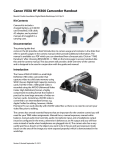
2.6.3. High Pressure Operation
When operating at high pressure, the increased density of gas will cause natural convection to flow
through the sensor tube if the instrument is not mounted in a level position. This natural convection
flow will be proportional to the system pressure. This will be seen as a shift in the zero flow output
that is directly proportional to the system pressure.
Fig. 2.4
Span Error vs Pressure
(0.026" Sensor Tube)
2.0%
0.0%
-2.0%
Span Error (% reading)
-4.0%
-6.0%
-8.0%
-10.0%
-12.0%
-14.0%
Mean error
-16.0%
max
min
-18.0%
-20.0%
0
100
200
300
400
y = 9.8877E-11x33.4154E-07x - 28.3288E-05x +
500
600
700
800
900
1000
Pressure(psig)
300-302 Series
Page 10 of 31
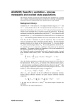
Span Error Vs. Pressure
Fig. 2.5
0.017" Sensor
5%
4%
Span Error (% reading)
3%
2%
1%
0%
Mean
Max
Min
-1%
-2%
0
100
200
300
400
500
600
700
800
900
1000
Pressure (psig)
If the system pressure is higher than 250 psig (1.7 MPa) the pressure induced error in the span reading
becomes significant. The charts above show the mean error enveloped by the minimum/maximum
expected span errors induced by high pressures. This error will approach 16% at 1000 psig. For
accurate high pressure measurements this error must be corrected.
The formulae for predicting mean error expressed as a fraction of the reading are:
Error26 = (9.887 * 10 −11 ) P 3 − (3.4154 * 10 −7 ) P 2 + (8.3288 * 10 −5 ) P, (0.026" Sensor )
Error17 = (1.533 * 10 -10 ) P 3 − (3.304 * 10 −7 ) P 2 + (1.8313 * 10 −4 ) P, (0.017" Sensor )
Where P is the pressure in psig and Error is the fraction of the reading in error.
The flow reading can be corrected as follows:
Corrected = Indication − ( Indication * Error )
Where the Indication is the indicated flow and Error is the result of the previous formula (or read from
charts above).
2.6.4. Blending of Gases
This section describes two methods by which to achieve a controlled blending of different gasses. Both
methods use the flow signal (Output) from one flow instrument as the Master to control the Command
signal (Input) to a second unit.
The first method requires that the two controllers use the same signal range (0 to 5 VDC or 4 to 20 mA)
and that they be sized and calibrated to provide the correct ratio of gasses. Then, by routing the
actual flow Output signal from the primary meter/controller through the secondary controller’s
300-302 Series
Page 11 of 31
External Input pin (See Tables 2.1 & 2.2), the ratio of flows can be maintained over the entire range of
gas flows.
EXAMPLE: Flow controller A has 0-100 slpm range with a 5.00 volt output at full scale. Flow
controller B has 0-10 slpm range with a 5.00 volt output at full scale. If flow controller A is set at 80
slpm, its output voltage would be 4.00 volts (80 slpm/100 slpm x 5.00 volts = 4.00 volts). If the output
signal from flow controller A is connected to the command Set Point of flow controller B, then flow
controller B becomes a slave to the flow signal of controller A. The resultant flow of controller B will
be the same proportion as the ratio of the flow ranges of the two flow controllers.
If the set point of flow controller A is set at 50% of full scale, and the reference voltage from flow
controller A is 2.50, then the command signal going to flow controller B would be 2.50 volts . The flow
of gas through flow controller B is then controlled at 5 slpm (2.50 volts/5.00 volts x 10 slpm = 5 slpm).
The ratio of the two gases is 10:1 (50 slpm/5slpm). The % mixture of gas A is 90.9090 (50slpm/55 slpm
and the % mixture of gas B is 0.09091% (5 slpm/55 slpm).
Should the flow of flow controller A drop to 78 slpm, flow controller B would drop to 3.9 slpm, hence
maintaining the same ratio of the mixture. (78 slpm/100slpm x 5v = 3.90v x 50% = 1.95v; 1.95v/5.00v
x 10 slpm = 3.9 slpm; 78 slpm: 3.9 slpm = 20:1)
In the blending of two gases, it is possible to maintain a fixed ratio of one gas to another. In this case,
the output of one flow controller is used as the reference voltage for the set point potentiometer of a
second flow controller. The set point potentiometer then provides a control signal that is proportional
to the output signal of the first flow controller, and hence controls the flow rate of the second gas as a
percentage of the flow rate of the first gas.
2.7. Output Filter
The output signal may have noise superimposed on the mean
voltage levels. This noise may be due to high turbulence in
the flow stream that the fast sensor is measuring or it could
be electrical noise when the flow meter has a high internal
gain. i.e. 5 sccm full scale meter. Varying levels of radio
frequency noise or varying airflow over the electronics cover
can also induce noise.
Fig. 2.6
JP-1
Noise can be most pronounced when measuring the flow
output with a sampling analog/digital (A/D) converter.
When possible, program the system to take multiple samples
and average the readings to determine the flow rate.
If less overall system noise is desired, a jumper may be
installed over the pins of JP-1 on the flow measurement
card. See Figure 2.6. Covering the pins closest to the “D”
connector will activate a resistor-capacitor (RC) filter that
has a time constant of one second. This will increase the
settling time of the indicated flow rate to approximately 4 seconds. Covering the other two pins will
lower the response time to approx. 1 second. This adjustment will not affect the calibration of the
flow meter circuit or the actual flow response to change in command signal (flow controllers). This
will only slow down the indicated response (output voltage/current).
2.8. Controlling Other Process Variables
Normally, a flow controller is setup to control the mass flow. The control loop will open and close the
valve as necessary to make the output from the flow measurement match the input on the command
line. Occasionally, gas is being added or removed from a system to control some other process
variable. This could be the system pressure, oxygen concentration, vacuum level or any other
parameter which is important to the process. If this process variable has a sensor that can supply an
analog output signal proportional to its value then the flow controller may be able to control this
variable directly. This analog output signal could be 0-5 volts, 0-10 volts (or 4-20 ma for units with 420 ma boards) or any value in between.
300-302 Series
Page 12 of 31
On the controller card there is a jumper that sets whether the control loop controls mass flow or an
external process variable. See Figure 2.7. If the jumper is over the top two pins, the loop controls
mass flow. If the jumper is over the bottom two pins, the loop controls an external process variable.
This process variable signal must be supplied on pin 12 of the D connector (for U pin out units) of the
measurement card. When the controller is set for external variable control it will open or close the
valve as necessary to make the external process variable signal match the command signal. The
command signal may be 0-5 volts, 0-10 volts (4-20 ma for 4-20 ma input/output cards) or any value in
between. If the process variable has a response time that is much faster or slower than the flow
meter signal it may be necessary to adjust the gain potentiometer.
2.9. Command Input
The flow controller will operate normally with any command input signal between 0-5 volts (4-20 ma
for units with 4-20 ma input/output cards) If the command signal exceeds ±14 volts it may damage the
circuit cards. During normal operation the control loop will open or close the valve to bring the output
of the flow meter signal to within ± 0.001 volts of the command signal. The command signal will not
match the flow signal if there is insufficient gas pressure to generate the desired flow. If the
command signal exceeds 5 volts the controller will continue to increase the flow until the output
matches the command signal. However, the flow output does not have any guaranteed accuracy
values under these conditions.
If the command signal is less than 2% of full scale (0.1 volts or 4.32 ma) the valve override control
circuit will activate in the closed position. This will force the valve completely closed regardless of
the flow signal.
2.10. Valve-Override Control
The valve override control line provides a method to override the loop controller and open or close the
valve regardless of the flow or command signals. During normal operation this line must be allowed to
float freely. This will allow the loop control to open and close the valve as it requires. If the valve
override line is forced high (> +5 volts) the valve will be forced full open. If the valve-override line is
forced negative (< -5 volts) the valve will be forced closed.
Fig. 2.7
2.11. Gain Potentiometer
On the top left of inlet side of the flow controller there is a hole
through which the gain potentiometer is accessible (Fig 2.3). This
gain potentiometer affects the gain of the closed loop controller.
Normally this potentiometer will be set at the factory for good
stable control. It may be necessary to adjust this potentiometer
in the field if the system varies widely from the conditions under
which the controller was setup. Turning this gain potentiometer
clockwise will improve stability.
Turning the potentiometer
counter-clockwise will speed up the valve reaction time to
changes in the command signal.
Gain Potentiometer
Control Loop Jumper
300-302 Series
Page 13 of 31
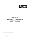
2.12. Temperature Coefficients
As the ambient temperature of
the instrument changes from
the original calibration
temperature, errors will be
introduced into the output of
the instrument. The
Temperature Coefficient of
Zero describes the change in
the output that is seen at zero
flow. This error is added to the
overall output signal regardless
of flow, but can be eliminated
by merely adjusting the zero
potentiometer of the flow
meter/controller to read zero
volts at zero flow conditions.
The Temperature Coefficient of
Span describes the change in
output after the zero error is
eliminated. This error cannot
be eliminated, but can be
compensated for
mathematically if necessary.
The curve pictured in Figure 2.8
shows the span error in percent
of point as a function of
temperature assuming 230C is
the calibration temperature.
300-302 Series
Fig. 2.8
Page 14 of 31
3. Theory of Operation
This section contains an overall functional description of the Hastings 300 series of flow instruments.
In this section and other sections throughout this manual, it is assumed that the customer is using a
Hastings power supply.
3.1. Overall Functional Description
The Hastings 300 meter consists of a sensor, base, and a shunt. In addition to the components in a
meter, The 300 controller includes a control valve and extra electronic circuitry. The sensor is
configured to measure gas flow rate from 0 to 5 sccm, 0 to 10 sccm, or 0 to 20 sccm, depending on the
customer’s desired overall flow rate. The shunt divides the overall gas flow such that the flow through
the sensor is a precise percentage of the flow through the shunt. The flow through both the sensor
and shunt is laminar. The control valve adjusts the flow so that the sensor’s flow measurement
matches the set-point input. The circuit board amplifies the sensor output from the two RTD’s
(Resistive Temperature Detectors) and provides an analog output of either 0-5 VDC or 4-20 mA.
3.2. Sensor Description
A cross section of the sensor is shown in Figure 3.1. The sensor consists of two coils of resistance wire
with a high temperature coefficient of resistance (3500 ppm/oC) wound around a stainless steel tube
with internal diameter of 0.6604 mm and 7.62 cm length. Each coil is 1.372 cm in length, and they are
separated by 1.27 mm distance. These two identical resistance wire coils are used to heat the gas
stream and are symmetrically located upstream and downstream on the sensor tube. Insulation
surrounds the sensor tube and heater coils with no voids around the tube to prevent any convection
losses. The ends of this sensor tube pass through an aluminum block and into the stainless steel sensor
base. This aluminum block thermally shorts the ends of the sensor tube and maintains them at
ambient temperature.
There are two coils of resistance wire that are wound around the aluminum block. The coils are
identical to each other, and are symmetrically spaced on the aluminum ambient block. These coils are
wound from the same spool of wire that is used for the sensor heater coils so they have the same
resistivity and the same temperature coefficient of resistance as the sensor heater coils. The number
of turns is controlled to have a resistance that is 10 times larger than the resistance of the heater
coils. Thermal grease fills any voids between the ambient temperature block and the sensor tube to
ensure that the ends of the sensor tube are thermally tied to the temperature of this aluminum block.
Aluminum has a very high thermal conductivity which ensures that both ends of the sensor tube and
the two coils wound around the ambient block will all be at the same temperature. This block is in
good thermal contact with the stainless steel base to ensure that the ambient block is at the same
temperature as the main instrument block and, therefore, the same temperature as the incoming gas
stream. This allows the coils wound on the aluminum block to sense the ambient gas temperature.
Two identical Wheatstone bridges are employed, as shown in Figure 3.2. Each bridge utilizes an
ambient temperature sensing coil and a heater coil. The heater coil and a constant value series
resistor comprise the first leg of the bridges. The second leg of each bridge contains the ambient
sensing coil and two constant value series resistors. These Wheatstone bridges keep each heater
temperature at a fixed value of dT = 48°C above the ambient sensor temperature through the
application of closed loop control and the proper selection of the constant value bridge resistors.
3.3. Sensor Theory
Consider the sensor design shown in Figure 3.1. The heat convected to or from a fluid is proportional
to the mass flow of that fluid.
Since the constant differential temperature sensor has 2 heater coils symmetrically spaced on the
sensor tube, it is convenient to consider the upstream and downstream heat transfer modes
separately. The electrical power supplied to either of the heater coils will be converted to heat, which
300-302 Series
Page 15 of 31
can be dissipated by radiation, conduction, or convection. The radiation term is negligible due to the
low temperatures used by the sensor, and because the sensor construction preferentially favors the
conductive and convective heat transfer modes. The thermal energy of each heater will then be
dissipated by conduction down the stainless steel sensor tube, conduction to the insulating foam, plus
the convection due to the mass flow of the sensed gas.
Because great care is taken to wind the resistive heater coils symmetrically about the midpoint of the
tube, it is assumed that the heat conducted along the sensor tube from the upstream heater will be
equal to the heat conducted through the tube from the downstream heater. Similarly, the heat
conducted from the upstream and downstream coils to the foam insulation surrounding them is
assumed to be equal, based on the symmetry of the sensor construction.
Since the sensor tube inlet and outlet are linked by an aluminum ambient bar, the high thermal
conductivity of the bar provides a ‘thermal short’, constraining the ends of the sensor tube to be at
equal surface temperature. Moreover, the tube ends and the aluminum ambient bar have intimate
thermal communication with the main flow passageway prescribed by the main stainless steel flow
meter body. This further constrains each end of the sensor tube to be equal to the ambient gas
temperature.
Further, since the length of each heater section is nearly 21 times greater than the inside tube
diameter, the mean gas temperature at the tubes axial midpoint is approximately equal to the tube
surface temperature at that point. Recall that the outside of the sensor tube is well insulated from the
surroundings; therefore the tube surface temperature at the axial midpoint is very close to the
operating temperature of the heater coils. The mean temperature of the gas stream is then
approximately the same as the heater temperature. Assuming the mean gas temperature is equal to
the heater temperature, it can be shown that the differential pressure is:
•
(3.1)
Pμ − Pd = 2 m C p (Theater − Tambient )
The value of the constant pressure specific heat of a
gas is virtually constant over small changes in
temperature. By maintaining both heaters at the
same, constant temperature difference above the
ambient gas stream temperature, the difference in
heater power is a function only of the mass flow
rate. Fluctuations in ambient gas temperature
which cause errors in conventional mass flow
sensors are avoided; the resistance of the ambient
sensing coil changes proportionally with the ambient
temperature fluctuations, causing the closed loop
control to vary the bridge voltage such that the
heater resistance changes proportionally to the
ambient temperature fluctuation.
Fig. 3.1
The power supplied to each of the 2 heater coils is
easily obtained by measuring the voltage across the
heater, shown as V2 on Figure 3.2, and the voltage
across the fixed resistor R1. Since R1 is in series with
the heater RH they have the same current flowing
through them. The electrical power supplied to a
given heater is then calculated:
(3.2)
Ρ=
(V1 − V2 )V2
R1
With a constant differential temperature applied to each heater coil and no mass flow through the
sensor the difference in heater power will be zero. As the mass flow rate through the sensor tube is
increased, heat is transferred from the upstream heater to the gas stream. This heat loss from the
300-302 Series
Page 16 of 31
heater to the gas stream will force the upstream bridge control loop to apply more power to the
upstream heater so that the 48oC constant differential temperature is maintained.
The gas stream will increase in temperature due to the heat it gains from the upstream heater. This
elevated gas stream temperature causes the heat transfer at the downstream heater to gain heat from
the gas stream. The heat gained from the gas stream forces the downstream bridge control loop to
apply less power to the downstream heater coil in order to maintain a constant differential
temperature of 48oC.
The power difference at the RTD’s is a function of
the mass flow rate and the specific heat of the
gas. Since the heat capacity of many gases is
relatively constant over wide ranges of
temperature and pressure, the flow meter may be
calibrated directly in mass units for those gases.
Changes in gas composition require application of
a multiplication factor to the nitrogen calibration
to account for the difference in heat capacity.
The sensor measures up to 20 sccm full scale flow
rate at less than 0.75% F.S. error. The pressure
drop required for a flow of 20 sccm through the
sensor is approximately 0.5 inches of H2O (125 Pa).
Fig. 3.2
3.4. Base
The stainless steel base has a 1.5" by 1.0” (38.1 mm by 25.4 mm) cross-section and is 3.64"(92.5 mm)
long. The length from face seal fitting to face seal fitting is 4.88” (124.0 mm). The base has an
internal flow channel that is 0.75"(19.1 mm) diameter. Metal to metal seals are used between the
base and endcaps, as well as the base and sensor module. Gaskets made of nickel 200 are swaged
between mating face seals machined into the stainless steel parts. All metal seals are tested at the
factory and have leak rates of less than 1x10-9 std. cc/s. Because of this corrosion resistant, all metal
sealed design, the Hastings 300 can measure corrosive gases, which would damage elastomer sealed
flow meters.
3.5. Shunt description
The flow rate of interest determines the size of the shunt required. As previously indicated, 9
separate shunts are required for the range of flow spanning 5 sccm to 10 slpm full scale. These shunts
employ a patented method of flow division, which results in a more linear flow meter. As a result, the
Hastings 300 flow meter calibration is more stable when changing between measured gases.
For the 5 sccm, 10 sccm, and 20 sccm flow rates a solid stainless steel shunt is used. The shunt uses a
close tolerance fit to block the main flow passage thereby directing all flow through the sensor tube.
The 50 sccm flow range uses a stainless steel shunt which has been machined flat on an edge. The gap
between the main flow passage and the flat machined on the shunt creates an alternate laminar flow
passage such that the overall gas flow is split precisely between the sensor and the shunt. By
increasing the number of flats and the size of the laminar shunt passageway, flow rates up to 200 sccm
are accommodated.
For flow rates above 200 sccm, the shunts are made so that an annular flow passage is formed between
the shunt cylinder and the main flow passage. A stainless steel plug with an annular spacing of
0.006"(0.15 mm) accommodates the 500 sccm flow range. Increased flow rates require larger gap
dimensions. Eventually, a maximum annular gap dimension for laminar flow is obtained (~0.020"(0.5
mm)). This patented shunt technology also includes inboard sensor ports which ensure laminar flow
without the turbulence associated with end effects. This unique flow geometry provides an
exceedingly linear shunt.
3.6. Shunt Theory
A flow divider for a thermal mass flow transducer usually consists of an inlet plenum, a flow
restriction, shunt and an outlet plenum. (See Figure 3.3) Since stability of the flow multiplier is
300-302 Series
Page 17 of 31
desired to ensure a stable instrument, there must be some matching between the linear volumetric
flow versus pressure drop of the sensor and the shape of the volumetric flow versus pressure drop of
the shunt. Most instruments employ
Poiseuille’s law and use some sort of
multi-passage device that creates
laminar flow between the upstream
sensor inlet and the downstream outlet.
This makes the volumetric flow versus
pressure drop curve primarily linear, but
there are other effects which introduce
higher order terms.
Most flow transducers are designed such
that the outlet plenum has a smaller
diameter than the inlet plenum. This
eases the insertion and containment of
the shunt between the sensor inlet point
and the sensor outlet point. If the shunt
is removed, the energy of the gas must be conserved when passing from the inlet
plenum to the outlet plenum. From Bernoulli’s equation, the sum of the kinetic
energy and the pressure at each point must be a constant. Since all of the pressure
drops are small, it can be assumed that the flow is incompressible.
Fig. 3.3
The pressure drop over the shunt can be shown to be:
(3.3)
4
⎡
⎤
1
2 ⎛ Di ⎞
⎟⎟ − 1⎥
ΔΡ a = ρVi ⎢⎜⎜
2
⎢⎣⎝ Do ⎠
⎥⎦
We can see that even with no effect from the shunt there will be a pressure drop between the sensor
inlet and outlet points. This pressure drop will be a strong function of the ratio of the two diameters.
Since the drop is a square function of the flow velocity the differential pressure will be non-linear with
respect to flow rate. Note also that the pressure drop is a function of density. The density will vary as
a function of system pressure and it will also vary when the gas composition changes. This will cause
the magnitude of the pressure drop due to the area change to be a function of system pressure and gas
composition.
Most of the shunts used contain or can be approximated by many short capillary tubes in parallel.
From Rimberg1 we know that the equation for the pressure drop across a capillary tube contains terms
that are proportional to the square of the volumetric flow rate. These terms come from the pressure
drops associated with the sudden compression at the entrance and the sudden expansion at the exit of
the capillary tube. The end effect terms are a function of density which will cause the quadratic term
to vary with system pressure and gas composition. The absence of viscosity in the second term will
cause a change in the relative magnitudes of the two terms whenever the viscosity of the flowing gas
changes.
(3.4)
ΔΡ a =
128μLQ 8ρQ
+ 2 4
πD 4
π D
2
(K C + K e )
The end effect for a typical laminar flow element, in air, account for approximately 4% of the total
pressure drop. For hydrogen, however, which has a density that is about 14 times less than air and
has a viscosity that is much greater than air, the second term is completely negligible. For the heavier
gasses, such as sulfur hexafluoride which has a density 5 times that of air, the end effects will become
10% of the total. This fundamental property makes it a difficult to maintain accuracy specifications
when calibrating an instrument using one gas for use with another gas.
The pressure drop is linear with respect to the volumetric flow rate between a point that is
downstream of the entrance area and another point further downstream but upstream of the exit
region. From Kays & Crawford, that entrance length (L ) of a capillary tube in laminar flow is a
function of the Reynolds number and the tube diameter. It can be shown that:
300-302 Series
Page 18 of 31
(3.5)
Le =
Qρ
5πμ
For a typical flow divider tube the entry length is approximately 0.16 cm. From this it can be seen
that if the sensor inlet pickup point is inside of the flow divider tube but downstream of the entrance
length and if the sensor outlet point is inside the flow divider tube but upstream of the exit point then
the pressure drop that drives the flow through the sensor would be linear with respect to volumetric
flow rate. Since the pressure drop across the sensor now increases linearly with the main flow rate
and the sensor has a linearly increasing flow with respect to pressure drop, there is now a flow through
the sensor which is directly proportional to the main flow through the flow divider, without the flow
division errors that are present when the sensor samples the flow completely upstream and
downstream of the flow divider.
Unfortunately, a typical shunt has an internal diameter on the order of 0.3 mm. This is too small to
insert tap points into the tube. Also, the sample flow through the sensor is approximately 10 sccm
while the flow through a shunt is approximately 25 sccm. This means the sample flow would be
affecting the flow it was trying to
measure. If the sensor tube is
made large enough, and with
enough flow through it to insert
the sensor taps at these
positions, then the pressure drop
would be too small to push the
necessary flow through the sensor
tube.
The solution is to use a different
geometry for the flow tube. It
must be large enough to allow
the sample points in the middle
yet with passages thin enough to
create the differential pressures
required for the sensor.
An
annular passage meets these
requirements.
Fig. 3.4
The basic operation is similar to the operation of the tubular shunt but the equations for the entry
length and pressure drop will be different.
If we assume that the annular region is very small, (Δr << r):
(3.6)
Cf=
24
Re
Then it can be shown that the pressure drop is:
(3.7)
P i − Po =
12QLμ
πτ (Δτ )3
The shunt must generate a pressure drop at the desired full scale flow which drives the proper flow
through the sensor tube to generate a full scale output from the sensor. Since the full scale flow of
the sensor is the same for all of the different full scale flows that may pass through the shunt, the
geometry must vary for the different full scale flows in order to generate the same pressured drop for
all of them. From Equation 3.7 it can be seen that if the width of the annular ring is varied slightly it
can correct for very large changes in the full scale flow rate (Q).
Below is a graph showing how the thickness of the annular ring must be changed to create a passage
that will properly divide the flow for various full scale flows. This graph is based on the 75 Pa pressure
drop required to push full scale flow through a particular sensor that has 2 cm spacing between the
inlet and outlet taps. The flow divider has an outside diameter of 0.95 cm.
300-302 Series
Page 19 of 31
Fig. 3.5
Thickness of the annular ring as a function of flow rate
for a sensor with a 75 Pa drop and a 2 cm spacing.
0.18
0.16
0.14
Passage Thickness (cm)
0.12
0.1
0.08
0.06
0.04
0.02
0
0
5
10
15
20
25
30
35
Flow (liter/min)
Each shunt must have a section of the annular region upstream of the upstream sensor tap to allow the
flow to become fully developed before reaching the first tap. The entry length for the annular passage
is then:
Le =
(3.8)
Qρ (Δr )
40πτμ
Below is a graph that demonstrates the entry length that would be required to design a flow divider for
various full scale flows. The parameters on the sensor that the flow divider must match are the same
as the ones on the previous graph.
Entrance length as a function of flow rate
for an annular ring of the size specified in figure 3.5.
Fig. 3.6
4.5
4
3.5
Entrance Length (cm)
3
2.5
2
1.5
1
0.5
0
0
5
10
15
20
25
30
35
Flow (liter/min)
300-302 Series
Page 20 of 31
3.7. Control Valve
Fig. 3.7
The control valve is an “automatic metering solenoid” valve (see Figure 3.7). While most solenoid
valves operate in either the fully open or closed positions, the automatic metering solenoid valve is
designed to control flow. A spring is used to hold a magnetic plunger assembly tightly against an
orifice, thereby shutting off the flow. The magnetic plunger assembly is surrounded by a coil of
magnet wire. When the coil is energized the electric current passing through the wire coil produces a
magnetic field which attracts the plunger. The plunger assembly moves away from the orifice allowing
the gas flow to pass between the orifice and the plunger seat. The distance between the orifice and
the plunger seat, and thus the flow through the valve, is controlled by the amount of current supplied
to the coil.
The valve seat is made of Kalrez (or equivalent) per fluoroelastomer. The valve orifice is made from
Stainless Steel. The valve plunger and pole piece are made of nickel plated magnetic alloy (Hi-perm
49) and the control springs are made of 302 stainless steel. Nickel gaskets seal all interfaces between
the process gas and the outside environment, as described in section 3.4.
3.8. Electronic Circuitry
The Hastings 300 employs a thermal transfer principle (capillary tube described in section 3.2) to
measure the flow through the sensor which is proportional to the total flow through the instrument.
The sensor develops a differential voltage output signal proportional to flow, which is amplified to
produce 5 VDC at full scale flow. The amplified output can be measured on the external “D”
connector. If a Hastings power supply is employed, the 5 volt output is also sent to the terminals on
the back and to the decoding circuitry in the display, the optional 4-20 mA analog output is available
in lieu of an output voltage. The addition of a 4-20 mA current loop transmitter on a secondary PC
board (mounted parallel to the main pc board) is required to provide this current loop. A jumper
change is made on the secondary PC board to establish the selected output mode.
300-302 Series
Page 21 of 31
4. Maintenance
This section contains service and calibration information. Some portions of the instrument are
delicate. Use extreme care when servicing the instrument. Authorized Maintenance
With proper care in installation and use, the instrument will require little or no maintenance. If
maintenance does become necessary, most of the instrument can be cleaned or repaired in the field.
Most procedures may require recalibration. Do not attempt these procedures unless calibration
references are available. Entry into the sensor or tampering with the printed circuit board will void
warranty. Do not perform repairs on these assemblies while the unit is still under warranty.
4.1. Troubleshooting
Symptom: Output reads strong indication of flow with no flow present. Zero pot has no effect.
Cause:
Power shorted out.
Action:
Turn power supply off for a few seconds, and then turn it on again. If this is ineffective,
disconnect the power supply from the unit. Check that the power supply voltages
are correct. Incorrect voltages most likely signify a faulty regulator chip inside the
supply. If the power supply display returns to zero after the instrument has been
disconnected there may be a short from the unit to ground.
Symptom: Hastings 300 output continues to indicate flow with no flow present, or indicates
±14 volts. Power supply inputs are correct (see the above troubleshooting tip) and
zero pot has no effect.
Cause:
Faulty IC chip(s) on the main PC board.
Action:
Replace main PC board. (See sections 4.5 and 6.1)
Symptom: Output of flow meter is proportional to flow, but extremely small and not correctable
by span pot.
Cause:
Sensor is not being heated.
Action:
Shut off gas supply and disconnect the power to the flow meter. Remove cover and
PC board from unit. Check the resistance from pins 1 to 2, and 3 to 4 (refer to
figures in section 6) of the sensor module. These pins should read 1650 Ω nominal
resistance. Also check that the resistance from pins 5 to 6, and 7 to 8 are 400 Ω
nominal value. Incorrect resistance values indicate that the sensor unit needs to be
replaced.
Symptom: Sensor has proper resistance readings, but little or no output with flow.
Cause:
Plugged sensor.
Action:
Shut off gas supply and disconnect the power to the flow meter. Remove cover and
PC board from unit. Remove and inspect sensor. If sensor has evidence of clogging,
clean or replace as applicable.
Symptom: flow meter reads other than 0.00 VDC with no flow or there is a small flow when the
flow meter reads 0.00 VDC.
Cause:
300-302 Series
Zero pot is out of adjustment.
Page 22 of 31
Action:
Shut off all flow. For the standard 0-5VDC output, adjust the zero potentiometer
located on the upper right inlet side of the flow meter until the meter indicates zero.
For the optional 4-20 mA output, adjust the zero potentiometer so that the meter
indicates slightly more than 4 mA, i.e. 4.03 to 4.05 mA. This slight positive
adjustment ensures that the 4-20 mA transmitter is not in its cut-off region. The error
induced by this adjustment is approximately 0.3% of full scale.
Symptom: Flow meter is out of calibration and non-linear.
Cause:
Leaks in the gas inlet or outlet fittings.
Action:
Check all fittings for leaks by placing soap solution on all fittings between gas supply
and final destination of gas. Check flow meter for leaks. Replace if required or
recalibrate as necessary.
Symptom: Little or no flow, even when the valve is in over-ride OPEN.
Cause:
Blocked orifice or incorrect pressure across the Flowcontroller
Action:
Verify that the pressure drop originally specified on the instrument is across the
instrument. If the differential pressure across the instrument is correct, the orifice may
be obstructed. Remove all gas pressure and shut off power supply. Remove the valve.
4.2. Adjustments
4.2.1. Calibration Procedure
1.
Calibration must take place with cover firmly in place.
2.
Connect power to “D” connector as specified in Section
2.5. Allow the instrument to warm up for 60 minutes with
10% of full scale flow.
3.
Completely shut off the flow and wait for 2 minutes. For
the standard 0-5VDC output, adjust the zero
potentiometer located on the lower inlet side of the flow
meter until the meter indicates zero. For the optional 420 mA output, adjust the zero potentiometer so that the
meter indicates slightly more than 4 mA, i.e. 4.03 to 4.05
mA. This slight positive adjustment ensures that the 4-20
mA transmitter is not in its cut-off region. The error
induced by this adjustment is approximately 0.3% of full
scale.
4.
Turn on gas supply to inlet of instrument and adjust the flow rate to the desired full scale
flow as indicated by a reference flow meter/controller.
5.
Adjust Span pot until the indicated flow reads full scale (5.00VDC or 20 mA). Perform this
step only if a calibrated reference flow meter is available.
6.
Record flow meter/controller and flow reference outputs for flow rates of 20%, 40%, 60%,
80% and 100% and make sure data are within ± 0.75% 3σ of full scale.
Fig. 4.1
4.3. End Cap Removal
The end cap on the inlet side must be removed to gain access to shunt assembly. First remove power
and shut off the supply of gas to the instrument. Disconnect the fittings on the inlet and outlet sides
of the transducer and remove it from the system plumbing. Remove the four Allen head screws
holding the end cap to the instrument. Carefully remove the end cap, nickel gasket, spacer, and
shunt, noting their order and proper orientation. The shunt can be severely damaged if dropped.
Examine the shunt. If damaged, dirty or blocked, clean and replace as applicable. Reassemble in the
300-302 Series
Page 23 of 31
reverse order of disassembly. A new nickel gasket will be required. Secure the endcap with 65 in lb.
(7.3 N m) to 85 in lb (9.6 N m) of torque on each stainless steel socket head cap screw. Use of a
fastener other than the one mentioned here may result in leakage at the seal. Recalibration of the
Hastings 300 is necessary.
4.4. Printed Circuit Board Replacement
NOTE: This instrument contains static sensitive PC boards. Maintain static protection when handling
the PC boards.
In the event that any of the PC boards fail, they are easily removed from the instrument and replaced
with a spare. This ease in disassembly and replacement substantially reduces instrument downtime.
1.
Replacement of the 4-20 mA option PC board: Unplug the power cable from the instruments “D”
connector. Remove the fasteners and steel can. The 4-20 mA board is the PC board mounted by
a single screw. Remove the screw and lift off the 4-20 mA board. Be careful not to damage the
main board and 4-20 mA board connectors.
2.
Replacement of the main PC board: Unplug the power cable from the instruments “D”
connector. Remove the fasteners and steel can. Remove the 2 screws which fasten the main PC
board to the sensor module. Gently unplug the main board from the sensor (and from the
4-20 mA board, if present).
4.5. Sensor Replacement
Follow instructions for removing the PC board(s) as described in Section 4.5. Remove the 4 Allen head
cap screws that fasten the sensor to the main instrument base. Remove the sensor module from the
base, discarding the used nickel gaskets. New nickel gaskets are required for re-assembly.
To place an order or to obtain information concerning replacement parts, contact the factory
representative in your area. See the last page in this manual for the address or phone number. When
ordering, include the following information: Instrument model number, part description and Hastings
part number.
300-302 Series
Page 24 of 31
5. Gas Conversion Factors
Gas conversion factors (GCF’s) for gasses metered using Hastings Instruments products, can be found by
visiting the Hastings Instruments web site. The web address can be found at the end of this document.
The gas conversion factors (GCF's) provided by Hastings Instruments (HI) fall into five basic accuracy
domains that, to a large extent, are dependent on the method by which they are found. The following
table summarizes the different methods used to determine the GCF's. The table lists the methods in
decreasing order of the degree of accuracy that may be achieved when applying a conversion factor.
Methods Used to Determine Gas Conversion Factors
1. Determined empirically at Hastings Instruments
2. Calculated From NIST tables
3. Calculated using the virial coefficients of independent investigators' empirical
data using both temperature and pressure as variables.
4. Calculated from virial coefficients using temperature only.
5. Calculated from specific heat data at 0 C and 1 atmosphere
1. The most accurate method is by direct measurement. Gases that can be handled safely, inert gases,
gases common in the atmosphere, etc., can be run through a standard flow meter and the GCF determined
empirically.
2. The National Institute of Standards and Technology (NIST) maintains tables of thermodynamic
properties of certain fluids. Using these tables, one may look up the necessary thermophysical property
and calculate the GCF with the same degree of accuracy as going directly to the referenced investigator.
3 and 4. Many gases that have been investigated sufficiently by other researchers, can have their molar
specific heat (C'p) calculated. The gas conversion factor is then calculated using the following ratio.
GCF =
'
C pN
2
'
C pGasX
GCF's calculated in this manner have been found to agree with the empirically determined GCF's within a
few tenths of a percent. Data from investigations that factor in pressure as well as temperature, usually
supply a higher degree of accuracy in their predictions.
5. For rare, expensive gases or gases requiring special handling due to safety concerns, one may look up
specific heat properties in a variety of texts on the subject. Usually, data found in this manner applies only
in the ideal gas case. This method yields GCF's for ideal gases but as the complexity of the gas increases,
its behavior departs from that of an ideal gas. Hence the inaccuracy of the GCF increases.
Hastings Instruments continually searches for better estimates of the GCF's of the more complex gases
and regularly updates the list.
Most Hastings flow meters and controllers are calibrated using nitrogen. The conversion factors published
by Hastings are meant to be applied to these meters. To apply the GCF's, simply multiply the gas flow
reading and the GCF for the process gas in use. For example, to calculate the actual flow of argon passing
through a nitrogen-calibrated meter that reads 20 sccm, multiply the reading and the GCF for argon.
20 x 1.4047 = 28.094
Conversely, to determine what reading to set a nitrogen-calibrated meter in order to get a desired flow rate
of a process gas other than nitrogen, you divide the desired rate by the GCF. For example, to get a desired
flow of 20 sccm of argon flowing through the meter, divide 20 sccm by 1.4047.
20 / 1.4047 = 14.238
That is, you set the meter to read 14.238 sccm.
Some meters, specifically the high flow meters, are calibrated in air. The flow readings must be corrected
for the case where a gas other than air is flowing through the meter. In addition, there must be a
correction for the difference in the GCF from nitrogen to air. In this case, multiply the reading and the
ratio of the process gas' GCF to the GCF of the calibration gas. For example, a meter calibrated in air is
300-302 Series
Page 25 of 31
being used to measure the flow of propane. The reading from the meter is multiplied by the GCF for
propane divided by the GCF of air.
20 * (0.3499/1.0015) = 6.9875
To calculate a target setting (20 sccm) to achieve a desired flow rate of propane using a meter calibrated to
air, invert the ratio above and multiply.
20 * (1.0015/0.3499) = 57.2449
Gas conversion factors can be found at the Hastings Instruments web site.
http://www.teledyne-hi.com
Follow the link to Mass Flow Products and then to Gas Conversion Factors.
300-302 Series
Page 26 of 31
6. Volumetric Vs Mass Flow
Mass flow measures just what it says, the mass or number of molecules of the gas flowing through the
instrument. Mass flow (or weight per unit time) units are given in pounds per hour (lb/hour), kilograms
per sec (kg/sec) etc. When your specifications state units of flow to be in mass units, there is no
reason to reference a temperature or pressure. Mass does not change based on temperature or
pressure.
However, if you need to see your results of gas flow in volumetric units, like liters per minute, cubic
feet per hour, etc. you must consider the fact that volume DOES change with temperature and
pressure. To do this, the density (grams/liter) of the gas must be known and this value changes with
temperature and pressure.
When you heat a gas, the molecules have more energy and they move around faster, so when they
bounce off each other, they become more spread out, therefore the volume is different for the same
number of molecules.
Think about this:
The density of Air at 0°C is 1.29 g/liter
The density of Air at 25°C is 1.19 g/liter
The difference is 0.1 g/liter. If you are measuring flows of 100 liters per minute, and you don’t use
the correct density factor then you will have an error of 10 g/minute!
Volume also changes with pressure. Think about a helium balloon with a volume of 1 liter. If you
could scuba dive with this balloon and the pressure on it increases. What do you think happens to the
weight of the helium? It stays the same. What would happen to the volume (1 liter)? It would shrink.
Why is the word standard included with the volume terms liters and cubic feet in mass flow
applications?
A mass flow meter measures mass …and we know we can convert to volume.
To use density we must pick one (or standard) temperature and pressure to use in our calculation.
When this calculation is done, the units are called standard liters per minute (SLM) or standard cubic
feet per minute (SCFM), for instance, because they are referenced to a standard temperature and
pressure when the volume is calculated.
Using the example to the left, we can see a standard
liter can be defined differently. The first balloon
contains 0.179 grams of Helium at 0 °C and 760
Torr (density of 0.179 grams/liter). Heat up that
balloon to room temperature and the volume
increases, but the mass has not changed. The volume
is not 1 liter anymore, it is 1.08 liters.
So, to define a standard liter of Helium at 25 °C, we
must extract only one liter from the second balloon
and that liter weighs only 0.175 grams.
1 Liter
1.08 Liter
1 Liter
0 °C
0.179 grams/1
liter
25 °C
0.179 g/1.08
liters
25 °C
0.164 grams
300-302 Series
If a mass flow meter is set up for STP at 0 °C and
760 Torr, when it measures 0.179 grams of He, it
will give you results of 1 SLM. If a second meter is
set up for STP at 25 °C and 760 Torr, when it
measures 0.164 grams, it will give results of 1 SLM.
Page 27 of 31
7. Drawings and References
HFM-300 / HFC-302 Outline Drawing
(All dim. Are approximate)
300-302 Series
Page 28 of 31
Sensor and Main PC
Board
TRANSDUCER
HFM-300
Sectional View
SHUNT
ENDCAP
ENDCAP
300-302 Series
Page 29 of 31
TRANSDUCER
VALVE
ASSEMBLY
CONTROLLER
CARD
SHUNT
ENDCAP
300-302 Series
ENDCAP
HFC-302
Sectional View
Page 30 of 31
8. WARRANTY
8.1. Warranty Repair Policy
Hastings Instruments warrants this product for a period of one year from the date of shipment to be
free from defects in material and workmanship. This warranty does not apply to defects or failures
resulting from unauthorized modification, misuse or mishandling of the product. This warranty does
not apply to batteries or other expendable parts, or to damage caused by leaking batteries or any
similar occurrence. This warranty does not apply to any instrument which has had a tamper seal
removed or broken.
This warranty is in lieu of all other warranties, expressed or implied, including any implied warranty as
to fitness for a particular use. Hastings Instruments shall not be liable for any indirect or consequential
damages.
Hastings Instruments, will, at its option, repair, replace or refund the selling price of the product if
Hastings Instruments determines, in good faith, that it is defective in materials or workmanship during
the warranty period. Defective instruments should be returned to Hastings Instruments, shipment
prepaid, together with a written statement of the problem and a Return Material Authorization (RMA)
number.
Please consult the factory for your RMA number before returning any product for repair. Collect freight
will not be accepted.
8.2. Non-Warranty Repair Policy
Any product returned for a non-warranty repair must be accompanied by a purchase order, RMA form
and a written description of the problem with the instrument. If the repair cost is higher, you will be
contacted for authorization before we proceed with any repairs. If you then choose not to have the
product repaired, a minimum will be charged to cover the processing and inspection. Please consult
the factory for your RMA number before returning any product repair.
TELEDYNE HASTINGS INSTRUMENTS
804 NEWCOMBE AVENUE
HAMPTON, VIRGINIA 23669 U.S.A.
ATTENTION: REPAIR DEPARTMENT
TELEPHONE
TOLL FREE
FAX
E MAIL
INTERNET ADDRESS
(757) 723-6531
1-800-950-2468
(757) 723-3925
[email protected]
http://www.teledyne-hi.com
Repair Forms may be obtained from the “Information Request” section of the Hastings Instruments web
site.
300-302 Series
Page 31 of 31