Download Agilent Technologies U8001A Product specifications

Agilent
Instrumentation Laboratory
Exercise
Prof. Horizon Walker Gitano Briggs
and Goh Chin Yuan
Department of Mechanical Engineering
University Science Malaysia
Agilent Technologies
Contents
Introduction
1
Laboratory Exercise 1 2
Resistor codes, breadboard, and basic measurements using
Agilent data acquisition system 2
Apparatus 2
1.1 Introduction and objectives 2
1.2 Electrical safety 3
1.3 Resistor color codes 3
1.4 The breadboard (protoboard) 4
1.5 Connection to the DAQ device 8
1.6 Agilent VEE Student/Pro 10
Verifying and launching your module connection 10
Laboratory Exercise #1 14
Laboratory Exercise 2 15
Diode junction temperature measurement 15
Apparatus 15
2.1 Introduction and objectives 15
2.2 Circuit setup 16
2.3 VEE programming 16
2.4 Calibration procedure 18
2.5 Temperature display 19
Laboratory Exercise #2 22
Laboratory Exercise 3 23
Motor current characteristics 23
Apparatus 23
3.1 Introduction and Objectives
3.2 Circuit setup 24
3.3 VEE programming 24
3.4 Test procedure 28
Laboratory Exercise #3 29
23
Laboratory Exercise 4 30
Foto-optic measurements of speed and flicker
Apparatus 30
Instrumentation Laboratory Exercise
30
II
4.1 Introduction 30
4.2 Objectives 31
4.3 Circuit setup 31
4.4 VEE programming 32
4.5 Test procedure 39
Laboratory Exercise #4 41
Laboratory Exercise 5 42
Motor speed-torque characteristics 42
Apparatus 42
5.1 Introduction and objectives 42
5.2 Circuit setup 43
5.3 VEE programming 43
5.4 Test procedure 51
Laboratory Exercise #5 52
Laboratory Exercise 6 53
Passive filter measurements 53
Apparatus 53
6.1 Introduction and objectives
6.2 Circuit setup 54
6.3 VEE programming 55
6.4 Test procedure 57
Laboratory Exercise #6 59
Appendix A 60
Resistor color codes
Appendix B 62
U2351A pinout
60
62
Appendix C 64
Appendix error codes
III
53
64
Instrumentation Laboratory Exercise
Introduction
This manual is intended as a complement to an existing course in
PC- based instrumentation for university and polytechnic students.
The theory of the various measurements, signals, and measurement
techniques should be covered in the course component. This
laboratory component addresses the practical application of the
knowledge and techniques studied. The various laboratory exercises
have been designed to provide you with the full experience in
acquiring measurements with minimal components and wiring.
The objective of these exercises is to help you focus on:
• Wiring basic circuits and measurement systems.
• Programming the data acquisition system.
With minimal effort, you should be able to perform accurate
measurements using the latest technology in data acquisition systems.
Once you have completed this course you should be able to then
apply these measurement techniques in further studies requiring data
collection and analysis.
Instrumentation Laboratory Exercise
1
Laboratory Exercise 1
Resistor codes, breadboard, and basic measurements using
Agilent data acquisition system
Apparatus
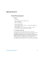
• Three units of 1 kΩ resistors
• Test/prototyping board
• Agilent U2351A, U2352A, U2353A, or U2354A USB multifunction
data acquisition device
• Agilent E3620A 50 W dual output power supply or Agilent
U8001A/U8002A single output DC power supply
1.1 Introduction and objectives
Welcome to the world of instrumentation and measurements. Things
you learn from this laboratory will provide a good foundation for
instrumentation and electronic measurements. The purpose of this
first laboratory exercise is to help you familiarize with laboratory
facilities, procedures, basic measurement techniques, and Agilent VEE
Student/Pro programming.
The specific objectives are:
• Observe the demonstration of Agilent VEE that you will use in your
laboratory exercises.
• Learn how to construct basic electrical circuits using breadboard.
• Learn how to properly acquire voltage measurements in circuit.
• Learn the resistor color code scheme necessary to read resistor
values and tolerances.
2
Instrumentation Laboratory Exercise
1.2 Electrical safety
Electrical voltages and currents can be dangerous if they occur at
values that interfere with physiological functions. All of the laboratory
exercises described in this manual are designed to use AC and DC
voltages of less than 15 V. Extra precaution must be taken when
dealing with high voltage lines (240 Vrms, 110 Vrms). Unless you are
trained in dealing with these higher voltages ensure that you never
accidently connect your circuits to a live line voltage.
1.3 Resistor color codes
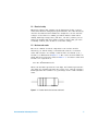
The most common electrical component is the resistor. In this
laboratory, we will be using ¼ W axial- lead resistors. A resistors
value and tolerance are usually coded in with color bands (a, b, c,
tolerance) as illustrated in Figure 1- 1. The colors used for bands are
listed with their respective values in Table 1- 1. A resistor's value and
tolerance are expressed as:
c
R = ab × 10 ±tolerance% Ω
Where the a band represent the tens digit, the b band represent the
ones digit, the c band represents the power of 10, and the tolerance
band represents the tolerance as a percentage of the coded resistance
value.
a b
c
Tolerance
Figure 1-1 Position of wire lead resistor color band
Instrumentation Laboratory Exercise
3
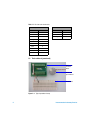
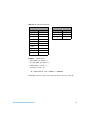
Table 1-1 Resistor color band codes
a, b, c Bands
Tolerance Band
Color
Value
Color
Value
Black
0
Gold
±5%
Brown
1
Silver
±10%
Red
2
Nothing
±20%
Orange
3
Yellow
4
Green
5
Blue
6
Violet
7
Gray
8
White
9
1.4 The breadboard (protoboard)
DAQ screw
terminal
block
Motor and
speed wheel
Protoboard
Figure 1-2 Typical protoboard setup
4
Instrumentation Laboratory Exercise
A breadboard (protoboard) shown in Figure 1- 2) is a device for
prototyping electronic circuits in a form that it can be easily tested
and changed. Figure 1- 3 illustrates a typical breadboard layout. The
the five holes in each half column (for example, row a through e) are
interconnected as shown in the figure. The lower half column (f
through j) is also interconnected, but is not connected with the upper
half column. The + and – rows that lie along the top edges of the
breadboard are also connected.
NOTE
• Always use the red wire for +5 V and the black wire for GND (0 V).
• To distinguish signals lines always use a different color for signals (for
example, white or yellow).
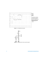
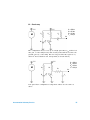
Figure 1- 3 also shows you how to construct a simple resistor circuit.
The schematic of the circuit is shown in Figure 1- 4. Push the
components legs into the appropriate holes on the breadboard to form
the circuit. You may run the components directly to the 5 V or
ground (GND) line if they require connection (rather than using a
separate wire for the connection as shown in the diagram). Also on
more complicated circuits it may be convenient to trim the
components legs slightly so they sit closer to the breadboard, rather
than allowing them to “float up in the air”. This will reduce the
possibility of accidental short- circuiting of component legs.
Instrumentation Laboratory Exercise
5
+
–
5V
GND
a
The grey lines indicate
the interconnection of
holes. The long 5 V and
ground lines are often
called “bus bars” of
“buses”.
e
f
j
+
–
Figure 1-3 Breadboard construction
5V
R1
Vdiv
R2
R3
Figure 1-4 Voltage divider circuit schematic diagram
6
Instrumentation Laboratory Exercise
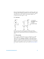
It is very important that you know how to acquire voltage
measurements properly. Figure 1- 5 shows two ways to connect the
voltage divider to the data acquisition system. The line going into
Screw Terminal Block pin 1 or pin 2 is the signal line. The line going
into pin 39 is the “ground reference” line, which we will connect to
ground 1 in our circuit. On the left the voltage divider Vdiv is
measured relative to ground. On the right both Vdiv and the 5 V line
can be measured.
5V
5V
Pin
1
R1
Vdiv
Pin
R1
Screw
Terminal
Block
Vdiv
39
R2
R3
1
2
39
R2
Screw
Terminal
Block
R3
Figure 1-5 Measurement of divider voltage (left) and independent measurement of
upper and lower voltages (right)
Instrumentation Laboratory Exercise
7
1.5 Connection to the DAQ device
The DAQ device must be properly connected to the circuit in order to
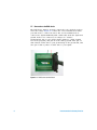
sense the voltage. Figure 1- 6 shows the screw terminal block where
you will need to connect the wires. The screw terminal block is
connected to Agilent USB DAQ with a SCSI cable. Both the signal and
ground needs to be connected, as voltages are “relative”
measurements. Pin 1 is the analog input channel 1 (called channel
101 in the program), and pin 39 is the analog ground. Wire pin 39
with a black or blue wire to your ground strip on the protoboard, and
wire pin 1 with a yellow or white wire to your signal.
Figure 1-6 DAQ screw terminal block
8
Instrumentation Laboratory Exercise
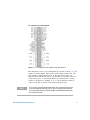
Pin configurations for U2351A, U2353A
Figure 1-7 Pin configurations for the DAQ screw terminal block
The full pinout of the screw terminal block is shown in Figure 1- 7. AI
stands for analog input. AI101 is the analog input channel 101 (the
first channel). AIH and AIL refers to the appropriate pins for
differential measurements, where you measure one voltage relative to
another. For most of our measurements we will measure a voltage
relative to ground (for example, 0 V), so the ground line must be
connected to pin 39 which is the analog input ground.
NOTE
As an example, the U2351A USB multifunction data acquisition device will be
used in the following laboratory exercise. You may subsitute the U2351A for
any of the following models: U2352A, U2353A, or U2354A USB multifunction
data acquisition devices.
Instrumentation Laboratory Exercise
9
1.6 Agilent VEE Student/Pro
Agilent VEE is a program which enables you to take measurements,
perform calculations, and display and save data into files. In
advanced applications the computer can be programmed to control
devices or processes based on the measured data.
To start, ensure that the U2351A USB multifunction data acquisition
(DAQ) device is powered on, and connected to the computer through
a USB cable.
Verifying and launching your module connection
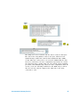
The Agilent Connection Expert is one of the utilities of the IO
Libraries. The Connection Expert configures the connected
instruments and enables communication. It is able to automatically
detect the U2351A devices plugged into the PC.
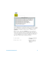
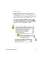
1 Go to Start > All Programs > Agilent IO Libraries Suite > Agilent Connection
Expert to launch the Connection Expert.
2 The detected U2351A will be visible on the Instrument I/O on this PC
explorer pane. Right- click on the U2351A instrument in the
explorer pane.
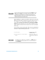
NOTE
Ensure that you do not remove the USB and power connection until the
firmware download has completed.
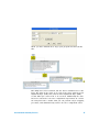
3 A context menu will appear. Select Send Commands To This Instrument.
4 The Agilent Interactive IO dialog box will appear. Click Send & Read
to send the *IDN? default command. The instrument’s response
should appear in the Instrument Session History panel.
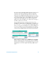
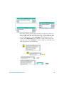
5 If the Connection Expert can successfully communicate with the
U2351A, this indicates that the instrument is installed correctly.
6 Double- click the Agilent VEE software icon on your desktop or go
to Start > All Programs > Agilent VEE Pro 8.5 > VEE Pro 8.5 to launch the
software.
10
Instrumentation Laboratory Exercise
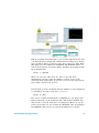
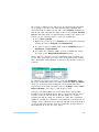
To fully utilize the capabilities of VEE programming you need to
master the various steps:
• Reading the input signal
• Signal processing (scaling, applying calibration factors, and so on)
• Displaying and saving the processed signal
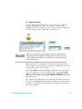
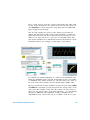
Figure 1- 8 shows a brief example of the various program segments.
• The Direct I/O box (left) is required for reading of the input signal.
• The Formula box (center) is used for signal processing.
• The Alpha Numeric box (right) is to display the resulting data.
Notice that there are inputs and outputs (small black squares on the
left and right hand sides of the boxes) for each of the boxes. In
general the inputs are on the left and outputs are on the right, so the
program has a left- to- right flow.
Figure 1-8 Program segments
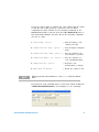
Double- click the < Double-Click to Add Transaction >, and a menu will
appear. Key in the following commands one line at a time:
1 "ROUT:SCAN, (@101)"
// Tells the DAQ to scan
channel 101 only
2 "SENS:VOLT:POL UNIP, (@101)"
// Sets the input to
unipolar mode
3 "SENS:VOLT:STYP SING, (@101)" // Sets the channel to be
read relative to ground
4 "SENS:VOLT:RANG 10, (@101)"
// Sets the channel to a
10 V maximum input
5 "MEAS:VOLT:DC? (@101)"
// Requests a DC
measurement of voltage
Instrumentation Laboratory Exercise
11
Change the WRITE tab to READ, then click OK to read the voltage in.
NOTE
You must enter the quote signs on lines 1 to 5, or it won't work! Also in line 6,
you need to select READ instead of WRITE and assign it to read a REAL64
type if it is not already chosen. Your voltage will automatically be assigned to
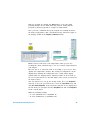
the variable X. You may also utilize the MultiInstrument Direct I/O box instead
of the Direct I/O box. The MultiInstrument Direct I/O box can be obtained by
clicking I/O > Advance I/O > MultiInstrument Direct IO. Your VEE program
should now look like Figure 1-9.
Figure 1-9 Program with completed input section
Link the boxes together in left- to- right order (for example, from “X”
to “A”, and then from “Result” to the AlphaNumeric box). To display
the real voltage, change the formula in the Formula box to “A” only
(for example, the output will be equal to A, which is the input).
Now you have your first program ready. Try to measure the voltage
across the resistors by clicking the RUN button (right pointing triangle
on the menu bar).
Wire up the electrical circuit as instructed above, and connect it to
5 V. If everything is working you should get a number around 1.6 in
the AlphaNumeric box at the right.
12
Instrumentation Laboratory Exercise
To calculate the difference in voltages you will need to read in 2
channels (101 and 102). Change all the lines in the Direct I/O box or
MultiInstrument Direct I/O box (left box) to (@101,102) instead of
(@101). Also add two additional lines:
1 "MEAS:VOLT:DC? (@102)"
2 READ:TEXT Y REAL64
On the Formula box right- click and ADD a DATA INPUT terminal. Link
the voltage from 101 into A, link channel 102 (Y output on the Direct
I/O box) into the new terminal B. Change the formula to “B- A” and
the result will be the difference. You can also add an alphanumeric
display of the raw voltages of 101 and 102 as well.
Figure 1-10 Program with two channels
Channel 1 (called X or 101) is reading the voltage divider Vdiv, which
should be approximately 1/3 of the supply voltage, or about 1.6V.
Channel 2 (called Y or 102) is measuring the supply voltage which
should be approximately 5 V. The equation calculates the difference
which should be around 3.4 V. This is the voltage drop across the
upper resistor in the divider circuit.
Instrumentation Laboratory Exercise
13
Laboratory Exercise #1
Test Report
NAME:______________________________
Part 1:
Calculate the equivalent resistance of the two resistors in parallel:
R = __________
Calculate the anticipated voltage across the resistors in parallel:
V = __________
Measure the voltage between the ground and the two lower resistors:
V = __________
Part 2:
Now set up the apparatus to measure the voltage drop across the upper resistor as well. Keep the previous measurement on
line, and add a measurement of the overall voltage (for example, ~5 V). The difference between these voltages is the drop
across the upper resistor.
Measure the voltage across the upper resistor:
i
ii
iii
iv
V = __________
Display the voltage across the resistors in parallel, and the whole voltage divider (for example, approximately 5 V).
Make a program which can calculate the voltage drop across the upper resistor, and display that voltage as well.
Now calculate the current through the circuit using I = V/R, assuming the upper resistor is exactly 1 kΩ.
Measure and display the current. Also measure the current draw reported by the power supply.
I (power supply) = __________
I (calculated) = __________
Call the technician and have him verify your setup:
Technician Check
Questions
Was the voltage that you calculated in Part 1 the same as what you measured?
Why could it be different?
14
Instrumentation Laboratory Exercise
Laboratory Exercise 2
Diode junction temperature measurement
Apparatus
• One 1 kΩ resistor
• One signal diode (silicon)
• Test/prototyping board
• Agilent U2351A, U2352A, U2353A, or U2354A USB multifunction
data acquisition device
• Agilent E3620A 50 W dual output power supply or Agilent
U8001A/U8002A single output DC power supply
• Thermometer (optional)
2.1 Introduction and objectives
The purpose of this laboratory exercise is to learn how to calibrate
and use a diode junction temperature sensor. A forward biased diode
should be assembled with a 1 kΩ resistor to +5 V. The diode voltage
(approximately 0.7 V) should be measured by the DAQ and displayed.
The voltage should be recorded when the diode is placed in contact
with container containing ice water (0 °C reference), as the 0 °C
value.
Next, the room temperature voltage should be recorded. Room
temperature should be measured with a thermometer, and the diodes
offset and span should be calibrated at 0 °C and at the measured
room temperature. The calculated diode temperature should then be
displayed on the screen in the form of a linear chart (like a
thermometer). Your body temperature should then be measured to
confirm that they are indeed alive.
Instrumentation Laboratory Exercise
15
2.2 Circuit setup
5V
R1 = 1 kΩ
D1 = Signal Diode
R1
VD
D1
VD will be fed into pin 1 of the DAQ board, and the circuit ground
will be fed into the ground (pin 39) of the DAQ. The diode has a
fixed polarity; it will not work if it is connected in the opposite
direction. The stripe end should be connected to ground.
Once the circuit is connected, confirm that you have +5 V and that VD
is approximately 0.7 V.
2.3 VEE programming
The voltage VD will change slightly with temperature. As the voltage
change is relatively small (a few mV), we should set up the DAQ for
the greatest sensitivity applicable to our measurement. The input can
be measured as bipolar (BIP, allowing both positive and negative
voltages) or unipolar (UNIP, allowing only positive voltages).
In this exercise, VD will always be positive, so using unipolar
configuration will allow us twice the resolution of bipolar mode. Also,
the input channels can be configured for various voltage input ranges.
Typically a 10 V input range is used, meaning that the maximum
input voltage is 10 V. In unipolar mode with a 16- bit analog to digital
converter, we then have a voltage resolution of 10 V/(216), or about
0.15 mV. As we know the diode junction voltage will be approximately
0.7 V, we can use an input voltage range of 1.25 V, greatly enhancing
our voltage resolution.
Instrumentation Laboratory Exercise
16
Set up the analog input on channel 101, and confirm that the signal
is read into pin 1 and ground is connected to pin 39. When
configuring the input channel use the following commands in the
MultiInstrument Direct I/O box (from the I/O > Advanced I/O menu or
from Instrument Manager side bar). Key in the following commands
one line at a time:
1 "ROUT:SCAN, (@101)"
// Tells the DAQ to scan
channel 101 only
2 "SENS:VOLT:POL UNIP, (@101)"
// Sets the input to unipolar
mode
3 "SENS:VOLT:STYP SING, (@101)" // Sets the channel to be
read relative to ground
4 "SENS:VOLT:RANG 1.25, (@101)" // Sets the channel to a
1.25 V maximum input
NOTE
5 "MEAS:VOLT:DC? (@101)"
// Requests a DC
measurement of voltage
6 READ TEXT Vd REAL64
// Reads the voltage as Vd
Make sure you enter a space between DC? and (@101) in line 5 or it will not
work!
Recall that the read command must be entered by double- clicking the
< Double-Click to Add Transaction > and changing it to the following:
Instrumentation Laboratory Exercise
17
2.4 Calibration procedure
We will perform a “two- point” calibration of the diode temperature
sensor. To calibrate the sensor you will need a small amount of ice.
Power up the circuit and display the voltage VD in an AlphaNumeric
box (found in the Display menu).
Allow the ice to come in contact with the diode and measure the
steady state voltage. You should notice that the diode voltage goes up
slightly when the ice is in contact with the diode. This should only
take a few seconds. Record this voltage as the “zero reference”, Vz.
Now remove the ice and allow the diode to warm up to the room
temperature. Measure the room temperature using the room
thermometer. In the absence of a thermometer you may assume the
room is at 25 °C. Record the steady state voltage, Vr of the diode
when it is at room temperature.
The calibration factor may now be calculated through:
CalFact = ( T room – T ice ) ⁄ ( V r – V z )
Where Troom is the temperature of the room in °C, and Tice is 0 °C.
The formula for converting the diode junction voltage to °C is then:
CalFact × ( V D – V Z )
Using the actual numbers (approximately 0.7 V for Vz and ∼1000 for
CalFact) fill out a formula box to perform the conversion. It should
contain a formula like:
– 1000 × ( A – 0.692 )
Where A is the voltage of the diode entering the formula box, and
0.692 is replaced by your 0 °C diode voltage.
Instrumentation Laboratory Exercise
18
2.5 Temperature display
Set up a Formula box (found in the Device menu) for calibration
allowing the subtraction of the “zero” reference voltage and
multiplication by the calibration factor as shown below. Display both
the raw voltage and the temperature converted to °C.
NOTE
Notice that a single output can be run into many inputs (as with Vd feeding
both the formula and 1st AlphaNumeric boxes). You can not, however, feed
several outputs into a single input, as this would cause a conflict: which input
value should be used?
This shows how the temperature conversion can be performed in a
single formula box. To make the program run continuously we need
to add some program “flow control”.
First add a Start button from the Flow menu. Place it in the upper
left of the screen as shown in the figure above. Next add an Until
Break loop from the Flow menu (Flow > Repeat > Until Break). Place it
below the Start button and wire the Start button into the top of the
Until Break box.
The output of the Until Break loop (right side) should be wired into
the top of the MultiInstrument I/O box as shown above. This tells the
program to repeatedly read and display the temperature until halted
by a stop command.
Instrumentation Laboratory Exercise
19
Run the program by clicking the Start button or the run (right
pointing triangle on the main menu bar) button. Verify that the
program accurately responds to changes in temperature.
Once you have confirmed that your program successfully measures
the diodes temperature, add a thermometer- type linear bar graph to
the display (found in the Display > Indicators menu):
Ensure that it reads near room temperature when you are not
touching the diode, and heats up to over 30 °C when clasped between
your fingers.
The last step is to add some form of recording so you can see how
quickly the temperature changes. The change in temperature can be
displayed by running the temperature into a Strip Chart display
(found under the Display menu). Add this feature at the bottom of
the screen and stretch it to the full width of the screen (as shown in
the figure below).
Also you will need to set up the X and Y axis. Go to the Properties
side bar on the left (you will need to select the Strip Chart first) and
click X, Y, Scales Properties. If the Properties side- bar is not displayed at
the left then you can right- click the Strip Chart box and click Properties
in the context menu.
Make the following setting:
• Y scale: minimum 20 to maximum 40.
• X scale: minimum 0 to maximum 200.
Instrumentation Laboratory Exercise
20
Ensure that Autoscaling is OFF. Finally, run your program and confirm
that you can record the temperature fluctuations as you touch and
release the diode.
Instrumentation Laboratory Exercise
21
Laboratory Exercise #2
Test Report
NAME:______________________________
Measure the Zero Reference Voltage:
VZ = __________
Measure the Room Temperature Voltage:
Vr = __________
Write down the actual room temperature:
Troom = __________
Calculate the calibration factor (Troom – Tice)/(Vr-VZ):
CalFact = __________
Now set up to display the temperature continuously. Clasp your fingers around the diode and measure the temperature of your
hand.
Thand = __________ ° C
Measured temperature of hand:
Set up the Strip Chart display to display a history of the diode's temperature. What is the time constant for temperature change
of the diode?
t = __________ s
Call the technician and have him verify your setup:
Technician Check
Questions
With a 1.25 V input range and 16-bits, what is the voltage resolution?
Given your calibration factor, what is the temperature resolution in °C/step?
Instrumentation Laboratory Exercise
22
Laboratory Exercise 3
Motor current characteristics
Apparatus
• One 0.5 Ω, 5 W resistor
• Small permanent magnet (PM) DC motor
• Test/prototyping board
• Agilent U2351A, U2352A, U2353A, or U2354A USB multifunction
data acquisition device
• Agilent E3620A 50 W dual output power supply or Agilent
U8001A/U8002A single output DC power supply
3.1 Introduction and Objectives
The purpose of this lab is to measure the current (I) versus
voltage (V) characteristics of a permanent magnet DC motor. A small
DC motor will be supplied with power from a variable power supply.
The negative side of the motor will be connected to ground through a
5 W, 0.5 Ω current sense resistor. The voltage of the current sense
resistor and the motor voltage will be read into the DAQ system.
The difference in voltage will be calculated and displayed as the
Motor Voltage. The current sense resistors voltage will be converted
to a current by dividing by the resistance (0.5 Ω). This current will be
displayed as the Motor Current. On a two- dimensional graph, the
current will be plotted as a function of voltage.
The power supply will be set to various voltage levels (2 V, 3 V, and
4 V). Initially the motor will operate at its no- load speed. At each
voltage a frictional break (folded paper pad) will be applied to the
motors output disk, gradually slowing the motor to a stop. The break
should be applied such that it takes several seconds for the motor to
spin to a stop, during which time the motor voltage and current are
recorded and plotted.
Instrumentation Laboratory Exercise
23
This experiment is repeated for each of the mentioned voltages. The
resulting curves (a linear increase in motor current with applied load)
will be recorded in a graph and curve fit (offline). The slopes of the
curves will be compared. Additionally the armature resistance of the
motor will be calculated.
3.2 Circuit setup
V
Vm
R1 = 0.5 Ω, 5 W
M = 5 V PM-DC motor
M
Vi
R1
Vi will be fed into pin 1 of the DAQ board, Vm will go into pin 2, and
the circuit ground will be fed into the ground (pin 39) of the DAQ.
3.3 VEE programming
As in the previous exercises, the voltages will be read using the
Direct I/O command. Vi will come in on analog input 101, and Vm will
come in on analog input 102. Set them up as UNIPolar and SINGle
ended with a RANGe of 10 V. Set up a Formula box to calculate
Vm–Vi. Display this as Motor Voltage.
In a separate formula box calculate and display the motor current by
dividing Vi by 0.5. Now calculate and display the resistance of the
motor. This is the motor voltage divided by the motor current.
Instrumentation Laboratory Exercise
24
Remember to include a space after the question mark in the
MEAS:VOLT:DC? command. Once you have confirmed the program
runs and gives reasonable numbers add an X-Y plot (found under the
Display menu). Display the motor voltage as a function of motor
current. Wire current in as X (the upper left input), and motor
voltage as the Y (lower left input).
Instrumentation Laboratory Exercise
25
You may want to set up the scale on the X- Y plot. To do this,
right- click the plot, and select Properties on the pop- up menu. Go to
the left side bar and click Scale Properties and make the following
setting:
X scale (current): minimum 0 to maximum 0.5
Y scale: minimum 1.5 to maximum 4.5
Ensure that Autoscaling is off for both axes.
Run the program and build up several points on your plot. Rub your
finger against the disk gently slowing the motor to a stall, and watch
what happens with the current. You should see the current increases
significantly as the motor is slowed. You may also notice the voltage
drops somewhat.
Once you have confirmed the X- Y plot is correct, you can add a
routine to save the data to a file. Add a To File box (found under the
I/O > To menu). Right- click it and add two data inputs, label them A
and B. Click the To File: button and enter a file name like Lab3.xls.
Also click on the Clear File box to clear the file at the beginning of
every run.
NOTE
Choose a different file name or file location for each run you wish to save.
Finally, double- click and add a WRITE transaction to send TEXT format
information with an EOL turned on. In the dialog box enter the
following:
A, ", ", B
This indicates that the variable A will be written to the file followed
by a space, a comma, and another space, then the variable B. With
the EOL (End Of Line) turned on at the end, this will write your data
in two columns: A, B. This file can be displayed with Microsoft® Office
Excel with the Comma separator option selected.
Link A and B to the Motor Voltage and Current as shown:
Instrumentation Laboratory Exercise
26
Instrumentation Laboratory Exercise
27
3.4 Test procedure
Set the power supply voltage to 2 V, and allow the motor to spin up
to its maximum speed. Notice what happens to the numbers as you
apply a load to the motor. Using a piece of paper slowly apply
pressure to the motors disk until the motor stalls. Record the no- load
voltage, current, and resistance. Record these parameters for the
stalled case as well. Repeat this for 3 V and 4 V power supply
voltages. Record your results on the Test Report sheet. Save a few
seconds of data to a file and plot it in Microsoft® Office Excel. Verify
that it looks the same as what you saw on the screen.
You will notice that as the load on the motor is increased, the current
draw is increased. The torque of a permanent magnet DC motor is
directly proportional to the torque. Also you may note that the power
supply voltage drops some what as the current increases. This "droop"
varies with power supply design. Better quality power supplies have
less droop. Some of this voltage reduction is also caused by greater
voltage losses in the wires due to higher currents. For a given
resistance of wire doubling the current will double the voltage drop
across the wire, because V = I × R even for wires.
Instrumentation Laboratory Exercise
28
Laboratory Exercise #3
Test Report
NAME:______________________________
Set the power supply to 2 V, 3 V, and 4V. At each voltage, measure the motor voltage, current, and resistance when no load is
applied, and when the motor is stalled (for example, with a heavy load).
Fill out the following table:
Motor Voltage
Motor Current
Motor Resistance
V Power Supply
No-Load
Stalled
No-Load
Stalled
No-Load
Stalled
2
3
4
Display the Motor Current as a function of Motor Voltage.
Call the technician and have him verify your setup:
Technician Check
Questions
What is the real resistance of the motor?
Why does it (the real resistance) appear to change with the load?
What is the power supply “droop” (V/A)?
Instrumentation Laboratory Exercise
29
Laboratory Exercise 4
Foto-optic measurements of speed and flicker
Apparatus
• One 10 kΩ Resistor
• One Cadmium Disulphide (CdS) fotoresistor
• Test/prototyping board
• Agilent U2351A, U2352A, U2353A, or U2354A USB multifunction
data acquisition device
• Agilent E3620A 50 W dual output power supply or Agilent
U8001A/U8002A single output DC power supply
4.1 Introduction
The purpose of this laboratory exercise is to measure the frequency
response of the Cadmium Disulphide (CdS) fotoresistor, and to
measure the flicker frequency of fluorescent lights. The CdS cell is an
inexpensive light sensitive resistor. Its resistance may be on the order
of 100 Ω when fully illuminated, and as high as 100,000 Ω in
darkness.
The CdS cell will be mounted below the holes of the motor's disk. As
the motor spins the opaque portions of the index wheel will shield
the CdS cell from light, changing its resistance, and producing a
measurable voltage. This voltage will be measured (peak- to- peak) as
the motor speed is changed. The amplitude will be displayed on the
computer, along with the raw signal.
As the motor speed is increased the frequency increases, and the
amplitude of the signal will decrease due to the low- frequency nature
of CdS cells. You should measure the maximum reasonable frequency
(at which the amplitude is equal to 50% of the DC amplitude) of the
CdS cell. Finally, the background noise of the florescent light flicker
should be measured.
Instrumentation Laboratory Exercise
30
4.2 Objectives
In this laboratory exercise, you will learn how to:
• import entire wave forms,
• calculate various statistics from the wave forms, and
• plot the wave forms
4.3 Circuit setup
5V
R1
R1 = CdS Cell
R2 = 10 kΩ
VL
R2
VL will be fed into pin 1 of the DAQ board, and circuit ground will be
fed into the ground (pin 39) of the DAQ.
Instrumentation Laboratory Exercise
31
4.4 VEE programming
First, set up the analog input on channel 101, as done in previous
exercises. We want to read in VL as a full waveform or trace
consisting of many points acquired in rapid succession. Instead of
sampling the signal through the "MEAS:VOLT:DC?" command we will
have to set it up to read an array of points. We need to set up both
the number of points required as well as the frequency. Key in the
following commands one line at a time:
1 "SENS:VOLT:POL UNIP, (@101)"
// Sets the input to
unipolar mode
2 "SENS:VOLT:STYP SING, (@101)" // Sets the channel to be
read relative to ground
3 "SENS:VOLT:RANG 10, (@101)"
// Sets the channel to a 1
V maximum input
4 "ACQ:POIN 2000"
// Sets up to read 2000
points
5 "ACQ:SRAT 10000"
// Sets up read frequency
of 10 kHz
6 "ROUT:SCAN, (@101)"
// Tells the DAQ to scan
channel 101 only
7 "DIG"
// Starts the digitization
process
Instrumentation Laboratory Exercise
32
As the digitization process takes time (in this case 200 ms), we must
wait for the data to be read before we can display it so we will have
to include the following loop which waits for completion of the
digitization.
First we need to add another Until Break loop. It is fed from the
bottom of the first Direct I/O box. Its output (right side square) is
connected to another Direct I/O box which queries the DAQ device to
see if the digitization process has been completed. To do this you
must enter 2 lines into this second Direct I/O box:
1 "WAV:COMP?"
// Asks if the digitization
is complete
2 READ TEXT x STR
// Reads the answer in
TEXT form into the
variable x
Instrumentation Laboratory Exercise
33
NOTE
On the second line you will have to change the command to READ, and select
TEXT type data in a STRing (a series of letters) format. The variable “x” will
automatically be generated for you as an output on the right side of the
MultiInstrument Direct I/O box. This needs to be wired to an If/Then/ Else
Conditional box (found under the Flow menu).
When digitization is complete the variable x will have the text value
YES. In the In/Then/Else Conditional box it will be input (left side) as
the variable A, so to check for this condition you need to enter
A= = "YES" in the box. When this is true it will operate the Then
output which we will run to a Break box (found under the Flow >
Repeat menu). This will break out of the status checking loop, and
allow continued execution from the bottom end of the second Until
Break loop.
Now we must read the waveform data. This is done in a third Direct
I/O box, which is fed from the bottom of the second Until Break loop.
It needs to contain the following two lines:
NOTE
1 "WAV:DATA?"
// Requests the actual
waveform data
2 READ BINBLOCK VL WORD ARRAY:*
NOEND
// Reads the voltage as a
binary block array into
VL
• You will need to change the second line to a READ, and set
the format appropriately. Make sure you click the button to
read No END byte.
Instrumentation Laboratory Exercise
34
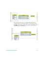
When you have finished these steps your program should look like
this:
This DAQ has 16- bit resolution, but the data is transferred as 8- bit
bytes. The data in the array VL is read as two bytes with the Least
Significant Byte (LSB) first, and the Most Significant Byte (MSB)
second. This byte order needs to be reversed. Additionally the data
has been converted to the twos complement sign format. To convert
the array back into a usable form you can perform a byte swapping
procedure, and simultaneously remove the twos complement offset.
Instrumentation Laboratory Exercise
35
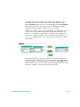
To do this, create the following formula boxes. The VL array is wired
into the left side, and the output at the right side is the array
converted to volts. The first formula box extracts the MSB and
removes the twos complement (by adding 128 to the value of the
array). The second formula box extracts the LSB. Notice we are using
a predefined function in the box called intpar. It returns the integer
part of a whole number. This is used to eliminate the fractional
component. The third formula box on the right reconstructs the
number in the proper form MSB × 256 + LSB, because each digit of
the MSB is equal to 256 of the LSB.
Also we divide by the factor of 217/Vrange where Vrange is the
maximum input voltage minus the minimum input voltage and 217 is
the number of voltage levels we can differentiate (for example, 0 to
216 + 215 + 214 + … + 2). As we have used a unipolar input with a
range of 10 V, therefore the maximum is 10 V and the minimum is 0
V, so Vrange is simply 10 V (if we had used bipolar Vrange would be
–10 V to +10 V, or 20 V), thus our conversion factor is 13107.2. This
is what the byte swapping routine and conversion should look like:
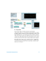
Finally, display the resulting data as a Strip Chart (under the Display
Menu) as shown below. Right click Strip Chart and select Properties
from the context menu. Go to the X- Y Scales properties on the left
side bar and set X minimum to 0 and maximum to 2000. Set Y scale
appropriately to see the trace. Ensure Autoscaling is OFF for both
scales.
Instrumentation Laboratory Exercise
36
Run the program and verify that it can read the signal from the CdS
cell. Move the motor slowly and confirm that the voltage level changes
from low when dark to a higher voltage when exposed to light. From
this graph you can estimate the maximum and minimum values, as
well as the frequency of periodic signals. Calculate the frequency from
the horizontal axis:
Freq = 1 ⁄ ( Period )
Where Period is the time from one wave to the next wave.
Alternatively you may count the number of whole cycles of the
waveform in the Strip Chart. If you have set the X scale properly the
trace will be 100 ms long (1/10 s).
Your frequency can be calculated from the number of cycles displayed
(n) divided by the time of the trace (0.1 s), or:
Freq = n ⁄ ( 0.1 )
For a more accurate measurement of amplitude we can apply some
built- in functions on the waveform data. Add another Formula box,
and feed the corrected array into it. Calculate the Mean. To get the
peak- to- peak value we can calculate the Maximum value and subtract
the Minimum value from it. Set up the Formula box as shown.
Instrumentation Laboratory Exercise
37
NOTE
You will have to right-click the box and add two additional data outputs, and
you will have to right-click and delete the Result output. Also you will have to
make sure the formula is entered properly as it calls the built in functions.
Display these values in AlphaNumeric display boxes.
Instrumentation Laboratory Exercise
38
4.5 Test procedure
Ensure that the sensor is placed beneath a hole in the motor's disk.
Measure the voltage when the CdS cell is fully illuminated. This is the
static light value. Now rotate the motor so the light is blocked.
Remeasure the dark static value of the voltage. Now spin the motor
up by applying 5 V to it. Notice what happens with the amplitude of
the signal. As the speed of the signal increases, the sensitivity of the
sensor is reduced, decreasing the peak- to- peak amplitude.
You can vary the speed of the motor by rubbing it with a piece of
paper. At several speeds stop the program and estimate the
peak- to- peak amplitude of the signal as well as the speed of the
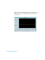
signal (in Hz). You should get data like the following (at low and high
speeds):
Instrumentation Laboratory Exercise
39
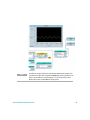
Finally, stop the motor and point the CdS cell at the fluorescent
lights (make sure to shield it from light from the window). Can you
detect the frequency of the lights? Below is a typical waveform
showing flicker.
Instrumentation Laboratory Exercise
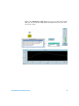
40
Laboratory Exercise #4
Test Report
NAME:______________________________
Measure the static dark voltage of the CdS cell circuit:
Vdark = __________
Measure the static light voltage of the circuit:
Vlight= __________
Calculate the expected peak-to-peak voltage for low frequencies:
Vp-p = __________
At what frequency does Vp-p drop to less than 50% of the static value:
Freq. = __________
What frequency do the fluorescent lamps flicker at?
Flicker = __________ Hz
Call the technician and have him verify your setup:
Technician Check
Questions
What is the cut-off frequency of this CdS cell (the frequency at which the output drops by 3 dB)?
What is the frequency of the AC voltage (line frequency) driving the fluorescent lamps?
Why is the flicker frequency different from the AC line frequency?
Instrumentation Laboratory Exercise
41
Laboratory Exercise 5
Motor speed-torque characteristics
Apparatus
• One 0.5 Ω, 5 W resistor
• Inferred reflective- type emitter/detector (IRPD)
• Small permanent magnet (PM) DC motor
• Test/prototyping board
• Agilent U2351A, U2352A, U2353A, or U2354A USB multifunction
data acquisition device
• Agilent E3620A 50 W dual output power supply or Agilent
U8001A/U8002A single output DC power supply
5.1 Introduction and objectives
The purpose of this lab is to measure the speed of a motor as a
function of input voltage. The motor spins an "index wheel" which has
eight regularly spaced holes near the periphery. A reflective type
inferred emitter- detector pair will detect these as they pass by.
The IR sensor should be aligned to give a nearly square wave output.
The frequency of this signal is eight times the motor's speed. The
motor voltage and speed signal will be read into the DAQ setup. You
will calculate the motor speed based on the frequency of the speed
signal and the number of transitions per revolution on the index
wheel. The raw signal and processed output (speed in rpm) should be
displayed, and the speed should be graphed as a function of motor
voltage on a two- dimensional plot.
The motor voltage should be varied from zero to the maximum setting
over the course of several seconds to get a good graph. Additionally
you should capture the "spin up and down" curves of the motor. To
do this the power supply should be set to the motors maximum
rating, and disconnected from the motor.
Instrumentation Laboratory Exercise
42
The speed and voltage should be recorded as a function of time, and
the motor voltage should be re applied to the motor causing it to spin
up rapidly. Once it attains full speed, the power should once again be
removed from the motor, and the speed should continue to be
recorded as the motor spins to a stop.
5.2 Circuit setup
5V
5V
R2
M
R3
Vi
R1
D1
R1 = 0.5 Ω, 5 W
M = 5 V PM-DC motor
R2 = 500 Ω
R3 = 50 kΩ
Vs D1 and Q1 are IRPD
Q1
Feed the sense resistor voltage (Vi) into channel 101 and the
foto- sensor voltage (Vs) into channel 102 of the DAQ. As always
ensure that the circuit ground is fed into the ground (pin 39) of the
DAQ.
5.3 VEE programming
The foto sensor channel will be set up as a unipolar, 10 V, single
ended (NRSE) input. Instead of sampling the signal through the
"MEAS:VOLT:DC?" command we will have to set it up to read an
entire trace or waveform. This is an array of data read from the
appropriate channel at a given frequency. We need to set up both the
number of points required as well as the frequency. To set it up use
the following commands the same way we did in Laboratory Exercise
4:
Instrumentation Laboratory Exercise
43
1 "ROUT:VOLT:POL UNIP, (@102)"
// Sets the input to
unipolar mode
2 "ROUT:CHAN:RANG 10 (@102)"
// Sets the channel to a
10 V maximum input
3 "ROUT:CHAN:STYP NRSE (@102)"
// Sets the channel to be
read relative to ground
4 "ROUT:SCAN (@102)"
// Tells the DAQ to scan
channel 102 only
5 "ACQ:POIN 1000"
// Sets up to read 1000
points
6 "ACQ:SRAT 80000"
// Sets up read frequency
of 80 kHz
7 "DIG"
// Starts the digitization
process
We must wait for the data to be read before we can display it, so we
will have to include a loop which waits for completion of the
digitization. The first Direct I/O box (called INITATE) sets up channel
102, and starts the digitization process. We then need to pole it to see
if it is ready. The second Until Break operates the Direct I/O box
called STATUS? Which asks "Is the wave complete?" ("WAV:COMP?")
and reads the answer as STAT (Status). If the DAQ device has not
finished, it loops on the STATUS? box, when completed it breaks out
to the third Direct I/O box, called DATA, which reads the data into an
array called RAW:
Instrumentation Laboratory Exercise
44
This DAQ has 16- bit resolution, but the data is read in 8- bit bytes.
The data in the array RAW is read as two bytes with the Least
Significant Byte (LSB) first, and the Most Significant Byte (MSB)
second. This byte order needs to be reversed. Additionally the data
has been converted to the twos complement sign format. To convert
the array back into a usable form you can perform a byte swapping
procedure, and simultaneously remove the twos complement offset. To
do this, create the following formula box. The RAW array is wired
into the left side, and the output at the right side is the array
converted to volts:
Instrumentation Laboratory Exercise
45
The sense resistor can be read as was done in Laboratory Exercise 3.
Put the Direct I/O box for reading the sense resistor after the wave
form reading box. Also notice the above byte reversal formulas have
been condensed into a single User Object (found under the Device
menu) called Array Convert. You will have to right- click the left and
right side bars of the User Object to add an input (for the RAW array)
and output for the converted array:
Instrumentation Laboratory Exercise
46
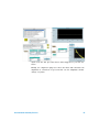
Power up the motor and read the sense resistor voltage, and the trace
from the foto- sensor. Display the foto- sensor trace in a Strip Chart
graph (found in the Display menu), and convert the sense voltage to
motor current by dividing by the resistance. Spinning the motor at
5 V with no load (without rubbing the spinning disk) you should get
like the following:
We now need to analyze the foto- sensor wave form to determine the
speed of the motor. The speed of the motor is related to the period of
the pulses (t) by the following:
Speed = 1 ⁄ ( n × t )
Where n is the number of pulses per revolution (eight in this case),
t is the period from one pulse to the next (in seconds) and Speed is
in Hz (cycles per second).
To calculate the period we need to loop through the data and
determine when the signal crosses a certain threshold value. The
threshold is a voltage that the signal crosses once each cycle. We
define our upper threshold (UT) as being half way between the
maximum value of the wave form and the average value of the wave
form. Placing the UT in the upper half of the signal reduces the
sensitivity to noise on the lower half of the wave form.
Instrumentation Laboratory Exercise
47
The period is defined as the time from one upward going transition
(or crossing) of the UT to the next upward going transition. The
waveform array is fed into the left side of the Array Stats formula box,
and the UT value exit from the right of the second formula Threshold
Limit box. The time from one upward going crossing to the next is one
period. Use the following steps to create the formula box:
1 Go to Device > Formula.
2 Right click on the box, go to Properties, go to Properties grid and
rename the title to Array Stats and Threshold Limit.
3 To create or delete terminal, right click the Formula box and go to
Add Terminal or Delete Terminal.
4 To rename the terminal, double click the terminal and change
the name at the Output Terminal Information window.
(Notice that we could also use two downwards going crossings and
get the same period, but you can not use an upward going crossing
and a downward going transition as this does not measure a full 1/8
rotation).
To calculate the period, you need to create two User Objects (Under
the Device menu). They will each require additional Inputs and Outputs
which are created by right- clicking the left and right side bars
respectively. In the first User Object place a For Range counter (Flow >
Repeat > For Range). Set it up to count from 0 to 990.
Next place an If/Then/Else box (in the Flow menu) and an Exit
UserObject box (from Flow menu). Wire it as shown with the array
fed into A and the UT fed into B. The For Range is a counter
stepping through the array one element at a time. The conditional
If/Then is checking for a transition. If a transition is encountered (for
example, array element B is less than the UT and array element B+1
is greater than UT) then the user object will exit, and the index of
the transition, B, is fed out of the object.
Instrumentation Laboratory Exercise
48
The second User Object does a very similar thing, but starts its
counting from the location B+1 (otherwise it would find the same
transition as the previous routine). Notice that the For Range box has
the FROM value as an input. You can add this by right- clicking the
left side of the box and adding it.
Instrumentation Laboratory Exercise
49
To obtain the period you must wire up the User Objects to the
incoming array, the UT, and feed the first index (from the object
named 1st Transit) value into the second User Object (called 2nd Transit).
The value needs to be incremented first by running it through a
formula box which simply calculates A+1 as its result.
Finally, the period is converted to rpm. There are eight holes, so each
cycle is 1/8 of a revolution. Reading at 80,000 Hz means that the
period of a revolution is eight times our period (B- A) divided by
80,000. The frequency (in Hz) of the revolution is then 80,000 / (8 ×
(B - A)), or simply 10,000 / (B - A). The speed in rpm is 60 times
this number.
Now that you have the period, convert it to actual speed in rpm.
Recall that rpm is equal to the speed in Hz times 60. Display motor
torque (current) as a function of motor speed in an X vs Y Plot (under
Display menu). Notice you can right clock this display and erase it at
any time, creating a clear motor speed- torque curve:
Instrumentation Laboratory Exercise
50
5.4 Test procedure
You are now ready to measure the motor's speed- torque
characteristics. This is a very important characterization of a motor
required for understanding how it will perform with a given load. Set
the supply voltage to 5 V, and run your program. There will be some
minor variation in the speed and torque, but it should be relatively
stable. Now slowly load the motors disk by pressing on it with a piece
of paper. Note what happens with the speed and the motor current.
As the speed decreases, the motor current should increase linearly.
This is the motors torque curve. It should look like a straight line
descending from the stall torque (at zero speed) to a smaller torque
at the no- load speed. Load the motor repeatedly, clearing the plot,
and notice the response.
Instrumentation Laboratory Exercise
51
Laboratory Exercise #5
Test Report
NAME:______________________________
What is the no-load speed of the motor with a 5 V supply:
RPMNL = __________
What is the no-load current of the motor with a 5 V supply:
INL= __________
What is the stall current of the motor:
Istall = __________
Give the equation for the best linear fit torque curve:
I = __________– RPM × __________
Get a good torque curve up on your screen and allow the technician to verify it.
Call the technician and have him verify your setup:
Technician Check
Questions
Why doesn’t the motor current resume to zero at no-load speed?
Can you recalibrate the speed measurement system to measure the duration of a single pulse (from a rising transition to the
subsequent falling transition)?
Given the number of points and data frequency, what are the maximum and minimum speeds that are accurately measurable
with this system?
Instrumentation Laboratory Exercise
52
Laboratory Exercise 6
Passive filter measurements
Apparatus
• One IRPD
• Small permanent magnet (PM) DC motor
• One 33 kΩ Resistor
• One 0.01 µf Capacitor
• Test/prototyping board
• Agilent U2351A, U2352A, U2353A, or U2354A USB multifunction
data acquisition device
• Agilent E3620A 50 W dual output power supply or Agilent
U8001A/U8002A single output DC power supply
6.1 Introduction and objectives
An AC signal will be generated from the motor and optical
interrupter setup as in the previous lab. As the motor speed is varied
the amplitude and frequency of the signal will be measured. A
high- pass filter will then be placed in series with the AC signal. The
amplitude will again be measured as a function of frequency. Next a
low- pass filter will be assembled, and the experiment will be
repeated. The three plots will be plotted on a common set of axis for
your analysis. They will measure the 3 dB point of the various filters.
Instrumentation Laboratory Exercise
53
6.2 Circuit setup
5V
5V
R1
M
R2
R3
Vflt
D1
R1 = 500 Ω
R2 = 50 kΩ
R3 = 33 kΩ
C1 = 0.01 µf
C1
Q1
The configuration above is set up as a high- pass filter. Vflt will be fed
into pin 1 of the DAQ board, and circuit ground will be fed into the
ground (pin 39) of the DAQ. For the low- pass filter R3 replaces C1,
which is moved between Vflt and ground (as shown below).
5V
M
5V
R1
D1
R2
R3
Q1
Vflt
R1 = 500 Ω
R2 = 50 kΩ
R3 = 33 kΩ
C1 = 0.01 µf
C1
Low- pass filter configuration. Component values are the same as
above.
Instrumentation Laboratory Exercise
54
6.3 VEE programming
The basic program is setup the similar to Laboratory Exercise 5. A
Start button is wired to an Until Break loop which runs a
MultiInstrument Direct I/O box (called INITIATE here). The last
command in this box is the DIGitization command, so next we
have to add in the loop (the second Until Break) requesting status
(the Direct I/O box asking for the WAVe complete STATus).
This loop repeats until the wave digitization has been completed,
which generates a Break, and continues the program execution,
proceeding to the MultiInstrument Direct I/O box (labeled DATA)
where the data is comes out as an array at RAW on the right side.
Also notice we want to read 2000 points at 80 kHz.
Instrumentation Laboratory Exercise
55
Place a strip chart to view the converted waveform. Also right click
it, and set the horizontal scale (found at the left side bar when you
click Properties) to 2000 points. The array must have the MSB- LSB
bytes swapped as previously.
Also we will calculate the period of the signal as previously, by
finding the first and second positive going transitions crossing the
upper threshold level UT. We are interested in the frequency of the
signal, so we will convert it to cycles per second (Hz) rather than
rpm. In the formula box we will divide 80,000 by the difference in the
transitions indices (for example, second index – first index).
To calculate the signals amplitude we could use the maximum value
minus the minimum value, but this would make us more susceptible
to individual noise spikes. Instead, we can first remove the offset of
the wave form, then calculate the Root Mean Square (RMS) value.
This is performed in a single formula box which we have named Offset
and RMS. The waveform is fed in along with the average value of the
wave form. The formula is then rms (B–A) where B is the array of
data, A is the average value of the data, and rms ( ) is a preexisting
function in VEE. This rms amplitude should be displayed in an
AlphaNumeric box, and fed into the Y coordinate of an X vs Y plot.
Instrumentation Laboratory Exercise
56
Similarly display the frequency as an AlphaNumeric box and feed it
into the X coordinate of the X vs Y Plot. Set up the X coordinate to
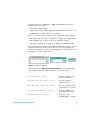
have a scale of 10 Hz to 100 Hz.
6.4 Test procedure
Once you have confirmed that you are reading the speed and
amplitude properly, clear the X- Y plot by right- clicking it and going to
Clear Display. Allow the motor to run at full speed. Slowly apply force
to the disk, slowing the motor. As the motor slows the frequency of
the signal will also be reduced.
When the high- pass filter is in place, lower frequencies will tend to
get filtered out. Thus, as the motor speed is reduced the amplitude of
the signal will be reduced. You should be able to clearly see this
trend as you slow the motor. Also notice the difference in the shape
of the wave form. Once you have completed this, have the technician
check your results and sign off your test sheet.
Now reconfigure the circuit in the low- pass configuration as per the
schematic above. The program should be the same, though you might
need to rescale some of the plots to get the data to fit nicely in the
window. If needed go to the Properties menu and reset the scale
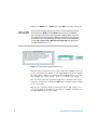
values. Repeat the experiment for the low- pass filter. Now the filter
will attenuate high frequencies, so the amplitude should increase as
the motor slows, as shown below.
Instrumentation Laboratory Exercise
57
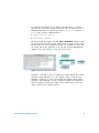
Again clear the X- Y plot and observe what happens as you slow the
motor.
Finally, for comparison purposes remove the filter and remeasure the
amplitude as a function of speed. In this case the amplitude should
change very little.
Instrumentation Laboratory Exercise
58
Laboratory Exercise #6
Test Report
NAME:______________________________
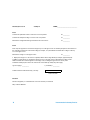
Measure the nominal signal amplitude (without a filter):
Vn = __________
Enter the appropriate amplitudes in the following table:
Signal Frequency
20 Hz
80 Hz
High-pass filter
Low-pass filter
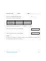
At approximately what frequency do the graphs cross?
Crossing freq. = __________ Hz
Call the technician and have him verify your setup (HIGH-PASS):
Technician Check
Call the technician and have him verify your setup (LOW-PASS):
Technician Check
Questions
Passive filters have cut-off frequencies of 1/2 pt where t is the time constant, RC. At what frequency should the filters cut-off?
Does the data agree with the theoretical cut-off frequency?
Instrumentation Laboratory Exercise
59
Appendix A
Resistor color codes
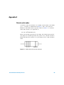
A resistor's value and tolerance are usually coded in with color bands
(a, b, c, tolerance) as illustrated in Figure 1. The colors used for
bands are listed with their respective values in Table 2. A resistor's
value and tolerance are expressed as:
c
R = ab × 10 ±tolerance% Ω
Where the a band represent the tens digit, the b band represent the
ones digit, the c band represents the power of 10, and the tolerance
band represents the tolerance as a percentage of the coded resistance
value.
a b
c
Tolerance
Figure A-1 Position of wire lead resistor color band
Instrumentation Laboratory Exercise
60
Table A-2 Resistor color band codes
a, b, c Bands
tolerance Band
Color
Value
Color
Value
Black
0
Gold
±5%
Brown
1
Silver
±10%
Red
2
Nothing
±20%
Orange
3
Yellow
4
Green
5
Blue
6
Violet
7
Gray
8
White
9
Example:
1kΩ Resistor
• First band (a): Brown = 1
• Second Band (b): Black = 0
• Third Band (c): Red = 2
• Tolerance: Gold = 5%
2
R = 10 ( 10 ±5% Ω) = 10 × ( 100 ±5% ) = 1000 ±5%
Individual resistor values can vary from about 950 Ω to 1050 Ω.
Instrumentation Laboratory Exercise
61
Appendix B
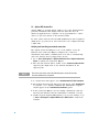
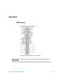
U2351A pinout
Pin configurations for U2351A, U2353A
Pin configurations for the DAQ screw terminal block
NOTE
(AIH101..108) and (AIL101..108) are for differential mode connection pair.
Instrumentation Laboratory Exercise
62
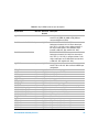
Table B-1 68-pin VHDCI connector pins descriptions
Signal Name
Direction Reference Description
Ground
AI_GND
N/A
N/A
Analog input (AI) ground. All three ground
references (AI_GND, AO_GND, and D_GND) are
connected together on board.
For 16 Channels: AI<101..116> Input
AI_GND
U2351A/U2352A/U2353A/U2354A
Analog input channels 101~116. Each channel pair,
AI<i, i+8>(i = 101..108), can be configured either as
two single-ended inputs or one differential input
(marked as AIH<101..108> and AIL<101..108>).
For 64 Channels: AI<101..164>
U2331A/U2356A/U2355A
Analog input channels 101~164). Each channel pair,
AI<i, i+32> (i = 101..132), is configured either as two
single-ended inputs or one differential input (marked
as AIH<101..132> and AIL<101..132>)
AI_SENSE
Input
AI_GND
Analog input sense. The reference pin for any
AI<101..116> or AI<101..164> channels in NRSE input
configuration.
EXTA_TRIG
Input
AI_GND
External AI analog trigger
AO201
Output
AO_GND Analog output channel 1
AO202
Output
AO_GND Analog output channel 2
AO_EXT_REF
Input
AO_GND External reference for AO channels
AO_GND
N/A
N/A
Analog ground for AO
EXTD_AO_TRIG
Input
D_GND
External AO waveform trigger
EXTD_AI_TRIG
Input
D_GND
External AI digital trigger
RESERVED
Output
N/A
Reserved pins. Do not connect them to any signal.
COUNT<301,302>_CLK
Input
D_GND
Source of counter <301,302>
COUNT<301,302>_GATE
Input
D_GND
Gate of counter <301,302>
COUNT<301,302>_OUT
Input
D_GND
Output of counter <301,302>
COUNT<301,302>_UPDOWN Input
D_GND
Up/Down of counter <301,302>
EXT_TIMEBASE
Input
D_GND
External Timebase
D_GND
N/A
N/A
Digital ground
DIO501<7,0>
PIO
D_GND
Programmable DIO of Channel 501
DIO502<7,0>
PIO
D_GND
Programmable DIO of Channel 502
DIO503<4,0>
PIO
D_GND
Programmable DIO of Channel 503
DIO504<4,0>
PIO
D_GND
Programmable DIO of Channel 504
Instrumentation Laboratory Exercise
63
Appendix C
Appendix error codes
While error codes reported by the software are rather cryptic, careful
reading of their descriptions may help you debug your program. Here
we have listed the appropriate error codes and their descriptions.
• Errors are retrieved in first- in- first- out (FIFO) order.
• Errors are cleared as you read them.
• If to many errors occurred, the last error stored in the queue (the
most recent error) is replaced with –350,"Error queue
overflow". No additional errors are stored until you remove
errors from the queue. If no errors have occurred when you read
the error queue, the instrument responds with +0,"No error".
• SYSTem:ERRor? will read and clear one error from the queue.
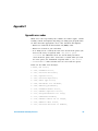
Below are the SCPI error messages:
• 0000, "No error",
• –100, "Command error",
• –101, "Invalid character",
• –102, "Syntax error",
• –103, "Invalid separator",
• –104, "Data type error",
• –108, "Parameter not allowed",
• –109, "Missing parameter",
• –110, "Command header error",
• –111, "Header separator error",
• –112, "Program mnemonic too long",
• –113, "Undefined header",
• –114, "Header suffix out of range",
• –120, "Numeric data error",
• –121, "Invalid character in number",
Instrumentation Laboratory Exercise
64
• –123, "Exponent too large",
• –124, "Too many digits",
• –128, "Numeric data not allowed",
• –130, "Suffix error",
• –131, "Invalid suffix",
• –134, "Suffix too long",
• –138, "Suffix not allowed",
• –140, "Character data error",
• –141, "Invalid character data",
• –144, "Character data too long",
• –148, "Character data not allowed",
• –150, "String data error",
• –151, "Invalid string data",
• –158, "String data not allowed",
• –160, "Block data error",
• –161, "Invalid block data",
• –168, "Block data not allowed",
• –200, "Execution error",
• –220, "Parameter error",
• –221, "Settings conflict",
• –221, "Settings conflict; amplitude and offset out of
reference voltage range",
• –221, "Settings conflict; high threshold is lower
than low threshold",
• –221, "Settings conflict; analog trigger level beyond
range because of analog trigger source",
• –221, "Settings conflict; sampling rate beyond range
because of number of channel",
• –221, "Settings conflict; acquisition points beyond
range because of number of channel",
• –221, "Settings conflict; waveform points beyond
range because of number of channel",
Instrumentation Laboratory Exercise
65
• –221, "Settings conflict; unsupported trigger mode",
• –221, "Settings conflict; unsupported trigger mode
because of analog trigger source",
• –222: Data out of range; external clock is set above
instrument's capability
• –223, "Too much data",
• –224, "Illegal parameter value",
• –300, "Device specific error",
• –310, "System error",
• –311, "Memory error",
• –313, "Calibration memory lost",
• –314, "Save/recall memory lost",
• –315, "Configuration memory lost",
• –321, "Out of memory",
• –330, "Self–test failed",
• –350, "Queue overflow",
• –400, "Query error",
• –410, "Query INTERRUPTED",
• –420, "Query UNTERMINATED",
• –430, "Query DEADLOCKED",
• –440, "Query UNTERMINATED after indefinite response",
• 112, "Channel list: channel number out of range.",
• 113, "Channel list: empty scan list",
• 222, "Settings conflict: module type does not match
state",
• 223, "Settings conflict: trig source changed to IMM",
• 261, "Not able to execute while scan initiated",
• 262, "Not able to abort scan",
• 263, "Not able to execute while instrument is
measuring",
• 264, "Not a scannable channel",
• 281, "Not able to perform on more than one channel",
Instrumentation Laboratory Exercise
66
• 301, "Module currently committed to scan",
• 303, "Module is not able to perform requested
operation",
• 304, "Does not exist",
• 305, "Not able to perform requested operation",
• 305, "Not able to perform requested operation; cannot
generate user–defined and pre–defined waveforms at
once",
• 305, "Not able to perform requested operation; output
is running",
• 305, "Not able to perform requested operation; output
has stopped",
• 305, "Not able to perform requested operation;
function must be enabled first"
• 305, "Not able to perform requested operation;
user–defined waveform not set",
• 305, "Not able to perform requested operation;
sampling rate cannot be 0 with user–defined output",
• 307, "Incorrectly configured ref channel",
• 308, "Channel not able to perform requested
operation",
• 308, "Channel not able to perform requested
operation: currently in differential mode",
• 309, "Incorrectly formatted channel list",
• 311, "Not able to specify resolution with Auto
range",
• 521, "Input buffer overflow",
• 522, "Output buffer overflow",
• 531, "Insufficient memory",
• 532, "Not able to achieve requested resolution",
• 602, "Self–test failed; RAM read/write",
• 626, "I/O processor failed self–test",
• 705, "Cal: aborted",
• 706, "Cal: value out of range",
Instrumentation Laboratory Exercise
67
• 747, "Calibration failed",
• 748, "Cal checksum failed, internal data",
• 748, "Cal: invalid while cal in progress",
• 748, "Firmware and FPGA revision mismatch"
Instrumentation Laboratory Exercise
68
www.agilent.com
Contact us
To obtain service, warranty or technical
assistance, contact us at the following
phone or fax numbers:
United States:
(tel) 800 829 4444
(fax) 800 829 4433
Canada:
(tel) 877 894 4414
(fax) 800 746 4866
China:
(tel) 800 810 0189
(fax) 800 820 2816
Europe:
(tel) 31 20 547 2111
Japan:
(tel) (81) 426 56 7832 (fax) (81) 426 56 7840
Korea:
(tel) (080) 769 0800 (fax) (080) 769 0900
Latin America:
(tel) (305) 269 7500
Taiwan:
(tel) 0800 047 866
(fax) 0800 286 331
Other Asia Pacific Countries:
(tel) (65) 6375 8100 (fax) (65) 6755 0042
Or visit Agilent World Wide Web at:
www.agilent.com/find/assist
Product specifications and descriptions in
this document are subject to change
without notice. Always refer to Agilent
Web site for the latest revision.
© Agilent Technologies, Inc. , 2008
First Edition, December 1, 2008
5990-3145EN
Agilent Technologies