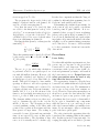
1
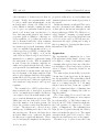
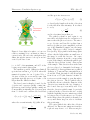
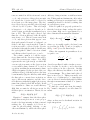
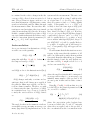
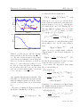
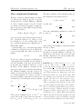
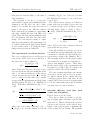
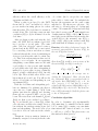
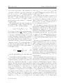
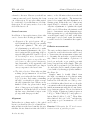
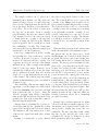
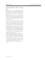
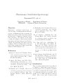
Fluorescence Correlation Spectroscopy
Experiment FCS - sjh, rd
University of Florida — Department of Physics
PHY4803L — Advanced Physics Laboratory
Objective
Fluorescence correlation spectroscopy describes a range of techniques that use the fluorescence of diffusing molecules to measure dynamical properties of those molecules, including their rate of diffusion, chemical reaction
rates, and more. You will use a basic setup
to study the diffusion of fluorescing polymer
nanospheres and fluorescing dye molecules to
calibrate the apparatus and learn about the
technique. Then, you will perform a biological
study on the opening and closing of genetically
engineered DNA hairpin loops.
References
R. Rieger, C. Rocker, G.U. Nienhaus, Fluctuation correlation spectroscopy for the advanced physics laboratory, Am. J. Phys.
73 1129-1134 (2005).
O. Krichevsky and G. Bonnet, Fluorescence
correlation spectroscopy: the technique
and its applications, Rep. Prog. Phys.
65 251-297 (2002).
Ted A. Laurence, Samantha Fore and
Thomas Huser, Fast, flexible algorithm
for calculating photon correlations, Optics Letters 31 829-831 (2006).
L.-L. Yang, H.-Y. Lee, M.-K.Wang, X.Y. Lin, K.-H. Hsu, Y.-R. Chang, W.
Fann and J.D. White, Real-time data
acquisition incorporating high-speed software correlator for single-molecule spectroscopy, J. of Microscopy 234 302-310
(2009).
Gr´egoire Bonnet, Oleg Krichevsky, and Albert Libchaber, Kinetics of conformational fluctuations in DNA Hairpin-loops,
Proc. Natl. Acad. Sci. USA, 95 86028606, July 1998 Biophysics.
D. Magde, E.L. Elson, and W.W. Webb,
Thermodynamic fluctuations in a reacting system: Measurement by fluorescence Introduction
correlation spectroscopy, Phys.
Rev.
There are many situations in biology where it
Lett., 29 705-708 (1972)
is desirable to characterize biomolecules (e.g.
E. Haustein and P. Schwille, Fluorescence proteins, nucleic acids, etc.) that are present in
correlation spectroscopy: Novel variations very small concentrations: How many copies
of an established technique, Ann. Rev. of a particular molecule are present? How
Biophys. Biomolec. Struct. 36 151-169 quickly does it diffuse through its environ(2007).
ment? How does it bind or interact with
FCS - sjh, rd 1
FCS - sjh, rd 2
other structures or chemical species that are
present? Ideally, the experimentalist would
be able to make such measurements on the
molecules inside a living cell. While it is already difficult to imagine counting the number of copies of a particular chemical species
inside a cell, it may seem even harder to believe that important physical and chemical
properties (such as diffusion coefficients, reaction equilibria, etc.) of these molecules can
also be measured inside the cell in a manner
that is non-destructive to both the cell and
the chemical species itself. Amazingly, all this
can be accomplished through fluorescence correlation spectroscopy (FCS), a technique that
was first described by Magde, et al. in the
early 1970s and then developed and advanced
intensively by a number of physicists during
the subsequent decades. FCS is remarkable
in part because the technique explicitly assumes and requires that the molecule of interest is present in very small numbers. Its invention was therefore an important early step in
the development of the many single-molecule
microscopy techniques that have subsequently
transformed cell biology since the early 2000’s.
It is now widely used, with new applications
and variations being invented and reported
regularly.
The essential idea of FCS is that when a
fluorescent molecule, or fluorophore, is present
at low concentrations in a sample, the fluorescence signal collected from that sample is subject to random fluctuations as the molecules
diffuse into and out of the field of view. The
fewer the number of molecules present, the
larger (in a relative sense) these fluctuations
become. The fluorescence collected from a
small group of diffusing molecules looks a lot
like random noise. However, the faster those
molecules diffuse, react, or interact, the faster
the fluorescence signal will fluctuate. Therefore, by studying the amplitude and frequency
October 20, 2014
Advanced Physics Laboratory
properties of that noise, we can determine fundamental physical and chemical properties of
the system.
In this experiment you will use FCS to measure the concentration and diffusion constant
of fluorophores, fluorescent nanospheres, and
fluorescently-tagged DNA. The DNA is a socalled “hairpin”, consisting of a single strand
of DNA that can bend around itself and form
a closed or end-to-end loop; FCS allows you to
characterize the rapid opening and closing of
this loop simply by observing the fluorescence
fluctuations of the DNA.
Apparatus
The experimental configuration for a basic
FCS apparatus is fairly simple. A laser beam
is brought to a sharp focus within a sample
containing a fluorophore and some of the fluorescent light is collected and sent to a photon
detector. Figure 1 shows the details for our
apparatus.
Two mirrors (not shown in Fig. 1) steer the
532 nm laser beam (green rays in the figure)
into the spatial filter. The spatial filter, which
smooths the laser beam intensity profile, consists of a focusing lens (L1, fl. = 40 mm),
which focuses the laser beam onto a pinhole
(P1, d = 20 µm) and then a collimating lens
(L2, fl. = 60 mm) re-collimates the beam exiting the pinhole.
The beam exiting L2 is steered into the
dichroic mirror (M1) using two more mirrors
(not shown in Fig. 1). The dichroic mirror reflects about 98% of the 532 nm laser light into
the back aperture of a microscope objective
(100×, oil immersion). The remaining laser
light (about 2%) passes through the dichroic
mirror and strikes the photodiode. The output
current from the photodiode is used to determine the incident laser power on the sample.
The microscope objective focuses the beam
Fluorescence Correlation Spectroscopy
sample
A
microscope
objective
pinhole
P1
dichroic (M1) L2
L1
M1
photodiode
removable
mirror
photon
detector
M2
F1 L3
camera
P2
pinhole
B
sample
microscope
objective
532 nm
laser
lens
L3
pinhole
P2
S1
S2
detector
Figure 1: (A) Optical configuration shows the
excitation laser (green rays), spatial filter (L1, P1,
L2), dichroic mirror (M1), microscope objective,
and photodiode. The objective brings the laser to
a focus within the sample. Fluorescence emission
from the sample (orange rays) is collected by the
objective and directed through a laser-blocking
filter F1 before it is focused by L3 onto the pinhole
P2 and then to the photon detector or, with the
removable mirror installed, onto the camera. (B)
The pinhole (P2) placed in the image plane allows
rays from point S1 in the sample to reach the
detector, but blocks rays arriving from S2 .
to a diffraction-limited spot within the sample,
exciting the fluorescence. Fluorescent emission is at wavelengths longer than the 532 nm
laser light (orange lines in the figure) and
some of it is collected and collimated by the
objective, which directs it back toward the
dichroic mirror (M1). The dichroic transmits
the longer wavelength light into a mirror (M2)
which steers it toward a laser-blocking (longpass) filter (F1) and a converging lens (L3,
fl. = 200 mm). This lens refocuses the light
onto the second pinhole (P2, d = 75 µm) after which is a photomultiplier tube (PMT) for
detecting individual photons getting through
FCS - sjh, rd 3
the pinhole.
A removable mirror can be placed in front of
P2 to divert the light onto a color CCD camera
that can be used for imaging the sample area.
These images can be used to determine the
magnification and for other diagnostics.
In addition to the fluorescent light from the
excitation volume, a fraction of the incident
laser light is reflected from the sample (or
from the microscope slide holding the sample) and is also collected by the objective.
The reflected laser light must be attenuated
or it would swamp the smaller intensity of the
fluorescence. As it passes back through the
dichroic mirror, roughly 98% of the 532 nm
laser is reflected back toward the source, while
most of the longer-wavelength fluorescent light
is transmitted through to the detector. The
longpass filter (F1 in Fig. 1) is needed to remove any residual laser light transmitted by
the dichroic.
The photon detector module (Hamamatsu,
H10682-110) contains a photomultiplier tube
(PMT), high voltage power supply, and pulse
processing electronics. Inside the PMT a lightsensitive photocathode emits an electron when
struck by a visible light photon. The emitted
electron is accelerated by a high voltage into
a second electrode where 5-10 electrons are
ejected and likewise accelerated into a third
electrode. Charge multiplication—each time
by a factor of 5-10—continues via a cascade of
collisions with an additional 10-12 electrodes
(dynodes) to produce a burst of 106 -108 electrons on the final electrode (anode). For each
incident photon, the module converts this anode charge into a single output voltage pulse
with an amplitude of 2 V and a width of 20 ns.
The frequency or rate of these pulses as a function of time will be denoted R(t) in the theory.
A key principle in FCS experimental design
is the need to minimize both the excitation
volume and the detection volume and to get
October 20, 2014
FCS - sjh, rd 4
the best possible overlap between them. The
detection volume is the region within the sample from which emitted light can reach the detector. The excitation volume is the region
within the sample, centered on the laser focal
spot, where the laser intensity is largest. If the
detection volume is too large, the PMT will,
in effect, detect the spatially-averaged concentration of fluorophores, rather than the locally fluctuating concentration. Fluctuations
in the detected light will be minimal and it
will not be possible to perform the analysis. If
the excitation volume is much larger than the
detection volume, diffusing fluorophores will
have been in the laser beam for some time before getting into the detection volume. This
pre-illumination has several unwanted effects
on the excitation-fluorescence process once the
fluorophores enter the detection region. If the
excitation and detection volume do not overlap well, many of the fluorescence photons will
go undetected and the signal will be weak.
Therefore, to generate a strong fluctuation signal, the laser excitation should be restricted to
the smallest possible volume within the sample, and the detector’s field of view must be
limited so that only photons from that small
volume are detected efficiently.
After excitation by the laser and subsequent
fluorescent emission, the fluorophore is ready
for another round of excitation-fluorescence.
When illuminated with a laser, typical fluorophores fluoresce at rates of 10 kHz or more.
However, the excitation can sometimes temporarily “shelve” the fluorophore in a longlived electronic triplet-state which will not
fluoresce again until the triplet state decays.
In addition, fluorophores in excited electronic
states can chemically interact with other fluorophores or surrounding molecules and become destroyed—permanently unable to participate in the excitation-fluorescence process.
These “burned out” fluorophores are said to
October 20, 2014
Advanced Physics Laboratory
be photobleached. A photobleached sample
will not fluoresce. The longer the exposure
to the laser light and the higher the laser intensity, the more likely the fluorophore is to
end up shelved or photobleached. Since both
processes lead to an average fluorescence that
is weaker than normal, it will also be important to use a laser power that is not any larger
than necessary to obtain a strong fluorescent
signal.
The beam exiting directly from the laser
has a somewhat irregular intensity profile and therefore—if focused by the microscope objective—will not focus to a sharp,
diffraction-limited spot. Inserting a spatial filter (L1, P1, L2 in Fig. 1A) smooths the intensity profile and consequently reduces the spot
size. One may think of the optical system as
using intense laser light to illuminate the pinhole aperture, and then projecting a sharp,
real image of that illuminated aperture onto
the sample.
We define a geometry where the microscope
slide is oriented parallel to the xy plane (see
Fig. 2), the laser beam propagates in the +z
direction, and the center of the beam focus is
r = 0. In the focal plane at z = 0, the laser
intensity pattern is reasonably well-described
by a Gaussian:
x2 + y 2
I(x, y, z = 0) = I0 exp −2
w02
where
!
(1)
2P
(2)
πw02
and P is the total laser power exiting the objective. I0 is the maximum intensity at the
center of the laser spot and w0 describes the
radius of the spot in the horizontal plane. The
prefactor of 2 in the argument of the exponential is traditional in laser optics formulas and
implies that the intensity a distance w0 from
the origin has dropped off by a factor of e−2 ,
I0 =
Fluorescence Correlation Spectroscopy
FCS - sjh, rd 5
and the spot size increases as
z
w2 (z) = w02 1 + (z/z0 )2
y
x Fluorescent
molecules
Laser beam
Figure 2: Laser light is brought to a focus on a
solution containing a low concentration of fluorescent molecules. The molecules emit light as they
diffuse through the intense focal region and are
excited by the laser beam.
i.e., to 14% of its maximum, and 86% of the
beam power is inside this radius.
The smallest possible (diffraction limited)
spot size has a radius w0 ≈ λ/2 N.A. where the
numerical aperture for our objective N.A. =
1.4 gives a value for w0 around 0.2 µm. Our
apparatus typically gives w0 ≈ 0.3 µm—a bit
larger than the diffraction limit.
The laser beam is sharply focused by the
objective and converges quickly coming into
the laser spot and diverges quickly coming out.
Consequently, its intensity also decreases away
from z = 0 and can be well modeled as follows
x2 + y 2
I(x, y, z) = I0 (z) exp −2
w(z)2
!
(3)
where the on-axis intensity I0 (z) falls off as
I0 (z) =
I0
1 + (z/z0 )2
(4)
(5)
z0 describes the length scale in the z-direction
for the fall-off in laser intensity. It is related
to w0 by
πw02
z0 =
(6)
λ
and is a few times larger than w0 .
The pinhole scheme is used again to ensure that only light from the excitation volume reaches the photon detector. The microscope objective and lens L3 together form a
microscope that projects a magnified, real image of the illuminated sample onto the image
plane. This is a so-called confocal configuration (see Fig. 1B); a pinhole in the image plane
allows only the light within one small area of
the image to reach the detector. Of course,
that light originates from the corresponding
region of the sample, and thus the pinhole prevents the detector from “seeing” other regions
of the sample. This detection area at the sample is a reduced or demagnified real image of
the pinhole P2. Our apparatus uses a pinhole
diameter of 75 µm and has a magnification of
about 100. Thus, the pinhole only allows light
from about a 0.75 µm diameter circular detection area at the sample to pass through to
the photon detector. The P2 pinhole size is
specifically chosen so that the diameter of the
detection area matches the 2w0 diameter of
the focused laser spot reasonably well. Note
that the detection pinhole must be precisely
positioned in the xy direction if it is to overlap
with the bright fluorescence emission spot that
is being produced by the microscope objective
in the image plane; the pinhole is mounted on
an xy micrometer stage in order to facilitate
this positioning.
The optics/pinhole also affect the collection
efficiency for fluorescent emissions from fluorophores away from z = 0. Fluorescent phoOctober 20, 2014
FCS - sjh, rd 6
tons are emitted in all directions and even at
z = 0, only a fraction of those photons emitted toward the objective will be collected by
it and sent on to the image plane. The fraction collected is proportional to the solid angle
collected by the objective. This solid angle
is largest at z = 0, where it depends on objective design, specifically its numerical aperture or NA. The solid angle collected, and
thus the collection efficiency, falls off rapidly
away from z = 0. This is because away from
z = 0, only those photons that appear—were
their path extended forward or backward—as
if they could have come from the 0.75 µm detection area will be collected by the objective
and make it through the pinhole. In this way,
the optics/pinhole define a detection volume
and efficiency that depends on x, y and z.
The volume common to both the excitation volume and the detection volume will be
called the measurement volume. Let dR(t)
represent the rate (photons/s) at which fluorescence photons arrive at the detector from
a very small volume element dV located at
a position r within the measurement volume.
dR(t) is determined by the product of the concentration C(r, t) of the fluorophore, the laser
beam intensity I(r), the efficiency with which
the fluorophore converts laser excitation energy to fluorescent emission, and the detection efficiency with which emitted photons are
turned into pulses by the PMT module. It will
be convenient to define an overall efficiency
Φ(r) that accounts for all factors except for
the fluorophore concentration. That is, we can
write
dR(t) = Φ(r)C(r, t)dV
(7)
Advanced Physics Laboratory
efficiency changes in time or with laser intensity. Taking such mechanisms into effect when
making predictions is non-trivial and so this
assumption should be checked by taking data
at several laser powers.
If the P2 pinhole is properly positioned so
that the detection volume overlaps the excitation volume, Φ(r) can be approximated by a
three dimensional measurement Gaussian
z2
x2 + y 2
−
2
Φ(r) = Φ0 exp −2
2
wxy
wz2
!
(8)
where wxy is roughly equal to the laser beam
spot radius (w0 in Eq. 1) and wz (roughly z0
in Eq. 4 and 5) is a few times larger.
Where the argument in parentheses above
is equal to one
x2 + y 2
z2
+
=1
2
wxy
wz2
(9)
describes an ellipsoid with a circular cross section of radius wxy in the x- and y-directions
and a radius wz in the z-direction. On this
ellipse, the efficiency has fallen to about 14%
of its maximum. The volume inside this el2
wz /3. Taking reasonable estilipse is 4πωwxy
mates: wxy = 0.4 µm and wz = 3 µm, fluorescence is detected as individual particles diffuse
through a measurement volume V ≈ 1 µm3 ≈
10−15 l or around 1 femtoliter.
To find the overall rate from the sample,
Eq. 7 must be integrated over all volume elements.
R(t) =
Z
d3 r Φ(r)C(r, t)
(10)
Equation 7 assumes that the fluorophore
emits fluorescent photons at a rate propor- where we have used a shorthand notation for
tional to the laser intensity at that point and triple integrations
nothing else. For example, it does not acZ
Z ∞ Z ∞ Z ∞
count for photobleaching, shelving, or any
d3 r =
dx dy dz
(11)
−∞ −∞ −∞
other mechanisms by which the fluorophore
October 20, 2014
Fluorescence Correlation Spectroscopy
FCS - sjh, rd 7
Theory
FCS can be used to study experimental samples that contain multiple species of fluorescent molecules with different concentrations
Ci and diffusion coefficients Di (where i =
1, 2, . . . , Nspecies ). Here, we develop the theory
of FCS for the simpler case in which the sample contains a single fluorescent species with
concentration C and diffusion coefficient D.
For multiple diffusing species the mathematics are more complex but not fundamentally
different. In the following we present a simplified (Nspecies = 1) version of the multiplespecies theory as presented by Krichevsky and
Bonnet.
In a well-mixed solution at chemical and
thermal equilibrium, the concentration of the
fluorescent species will have a uniform steadystate value C, where this value represents an
average over macroscopic scales of time and
distance. Over microscopic scales, however,
the particles are in continuous motion (diffusive, i.e., Brownian motion) and so when averaged over these much smaller length scales,
the concentration C(r, t) tends to fluctuate in
space and time. (See Figure 3.) The smaller
the averaging volume, the larger the fluctuations.
Fluctuations in the concentration are created continuously by random Brownian forces
while they simultaneously decay over time according to the diffusion equation
∂C(r, t)
= D∇2 C(r, t)
∂t
(12)
where D is the diffusion coefficient of the fluorescent molecules.
Note that we can also write C(r, t) as the
sum of its constant average C and its timeand space-dependent fluctuation δC(r, t):
C(r, t) = C + δC(r, t)
(13)
Figure 3: While the average concentration—
here, C ' 1 nM—remains constant, the instantaneous concentration of fluorescent molecules
C(r, t) averaged over a finite (but small) volume
fluctuates with time as the molecules diffuse in
and out of that volume.
With this definition, the temporal and spatial
averages of δC(r, t) will both be zero. Moreover, because C is constant, using Eq. 13 in
the diffusion equation 12 gives
∂δC(r, t)
= D∇2 δC(r, t)
∂t
(14)
Equation 14 describes a simple relationship
between the temporal and spatial behavior of
the fluctuations δC(r, t). At locations where
C is a maximum, i.e., where the second spatial
derivative of δC is negative), the time derivative of δC is negative, and so δC must decrease
in time. Further, the sharper the maximum in
δC, the more rapidly these local maxima dissipate. Conversely, where the second derivative
is positive so that δC is locally at a minimum,
the concentration must increase over time; local “gaps” in concentration tend to fill in over
time. In this way, Eq. 12 (or Eq. 14) state that
fluctuations or inhomogeneities in the concentration tend to smooth themselves out, and
that the rate of smoothing is faster where δC
has a steeper gradient.
As we will see, the most useful information
October 20, 2014
FCS - sjh, rd 8
Advanced Physics Laboratory
is contained in the relative changes in the fluorescence R(t) collected from an excited volume. The problem is to figure out how to extract that information: R(t) fluctuates continuously as individual particles diffuse through
the measurement volume. Because these fluctuations are random in time, there is not much
gained from studying R(t) directly. It is more
useful to examine statistical properties of R(t)
associated with its fluctuations as these can be
related to important physical parameters (D,
C, wxy , wz , etc.) of the experiment.
system and the measurement. The autocorrelation compares δR at a time t0 with its value
at a later time t0 + t (see Fig. 4). Suppose
that δR requires a time τ to change significantly. Consequently, for t < τ , δR(t0 + t)
is likely to have the same sign as δR(t0 ); the
product δR(t)δR(t0 + t) will usually be positive, thereby leading to G(t) > 0. However,
for t τ we expect that δR will have changed
considerably between t0 and t0 + t; δR(t0 + t)
will be equally likely to be positive or negative no matter what sign δR(t0 ) had; the product δR(t0 )δR(t0 + t) will be equally likely to
be positive or negative and it will average to
Autocorrelation
zero. Consequently, G(t) will approach zero
As we are interested in fluctuations of R(t), as t → ∞.
We will assume that the fluctuations are stawe will focus on the quantity
tionary, in the sense that the statistics of δR
δR(t) = R(t) − R
(15) will be no different if we study them now than
if we study them later this afternoon. (Assume
using this with Eqs. 10 and 13, defines R as that the sample doesn’t dry out!) In that case,
the temporal average of R(t)
the time t0 in Eq. 18 might as well be t0 = 0
Z
and we can rewrite Eq. 18 as
R = d3 rC Φ(r)
(16)
hδR(0)δR(t)i
(19)
G(t) =
2
and δR(t) as due to the fluctuations in C(r, t)
R
δR(t) =
Z
d3 r Φ(r)δC(r, t)
(17)
δR(t) changes randomly over time and we
anticipate that it will change more rapidly if
the particles diffuse more rapidly, or if the detection volume is smaller. Therefore, we wish
to characterize the time dependence of δR(t)
in a statistical way. A good way to do this is
to study the autocorrelation of δR(t), defined
as
G(t) =
hδR(t0 )δR(t0 + t)i
(18)
2
R
The angle brackets in the numerator indicate
an ensemble average, meaning an average over
many (hypothetical) implementations of the
October 20, 2014
where the angle brackets should be interpreted
as an expectation value, i.e., as an average over
infinitely many samples of the product of δR
at some point in time and its value a time t
later.
Using Eq. 17 in Eq. 19 tells us that, in order
to relate G(t) to the physical parameters D, C,
etc., we need to evaluate
G(t) =
1 Z
3
d3 r 0
(20)
R
Φ(r)Φ(r0 ) hδC(r, 0)δC(r0 , t)i
2
dr
Z
where the expectation value brackets have
been moved inside the d3 r and d3 r0 integrals
where they are applied only to the product of
the concentrations as the concentration is the
Fluorescence Correlation Spectroscopy
A
FCS - sjh, rd 9
for which the inverse transform is
1 Z 3 e
δC(r, t) =
d q C(q, t)e−iq·r
(2π)3/2
120
R(t)
100
80
60
δR(t’)
δR(t’+t)
40
t’
20
0
0
0.05
n
t’+t
0.1
0.15
0.2
0.25
Time (s)
(22)
where q · r = qx x + qy y + qz z and the shorthand notation is again used for the triple integration in q (d3 q = dqx dqy dqz , with integration limits from −∞ to ∞). Inserting Eq. 22
into the diffusion equation, Eq. 14, noting
that ∇2 e−iq·r = −q 2 e−iq·r (where, of course,
q 2 = q · q = qx2 + qy2 + qz2 ) gives
3.5
B
G(t)
2.5
2
1.5
tD
1
0.5
0
10 -5
10 -4
10 -3
10 -2
10 -1
!
e
∂ C(q,
t)
e
d qe
+ Dq 2 C(q,
t) = 0
∂t
(23)
For this equation to be true, the term in parentheses must be zero for all q and solving it
gives
2
e
e
C(q,
t) = C(q,
0)e−Dq t
(24)
Z
3
3
−iq·r
1
where, in order to satisfy initial conditions,
e
C(q,
0) must be the Fourier transform of
Figure 4: (A) The photon count rate R(t) fluc- δC(r, 0)
tuates randomly around its average value R. In1 Z 3
e
C(q,
0)
=
d r δC(r, 0)eiq·r (25)
set: The autocorrelation function G(t) charac3/2
(2π)
0
t (s)
terizes the average similarity between δR(t ) and
δR(t0 + t). For shorter intervals t, both δR are For the Fourier transform at least, we have
likely to be of the same sign, leading to a posi- found the time dependence of δC.
Now rewrite the expectation value using
tive G(t). For longer intervals t, the fluctuations
are uncorrelated and G(t) → 0. (B) The calcu- Eq. 22 and then Eq. 24
lated autocorrelation function (Eq. 54) is shown
hδC(r, 0)δC(r0 , t)i
for tD = 0.9 ms, ω = 1 and N = 0.34.
Z
1
0
e
δC(r, 0) d3 q e−iq·r C(q,
t)
3/2
(2π)
1 Z 3 −iq·r0 −Dq2 t
=
dqe
e
(26)
(2π)3/2
=
only quantity that fluctuates randomly. The
trick will be to calculate this expectation value
D
E
e
δC(r,
0)
C(q,
0)
using the diffusion equation for δC(r, t) and a
property of δC(r, t) related to Poisson statise
Using Eq. 25 to substitute for C(q,
0) (using
tics.
00
the dummy integration variable r as r and r0
We start by defining the Fourier transform are already in use) then gives
(in all three dimensions) of δC(r, t).
hδC(r, 0)δC(r0 , t)i
(27)
1 Z 3 −iq·r0 −Dq2 t Z 3 00 iq·r00
=
d qe
e
dr e
Z
(2π)3
1
e
C(q,
t) =
d3 r δC(r, t)eiq·r (21)
hδC(r, 0)δC(r00 , 0)i
(2π)3/2
October 20, 2014
FCS - sjh, rd 10
Advanced Physics Laboratory
As discussed in more detail below, the bracketed expression in the above integral is proportional to a delta function δ(r − r00 ). Together
with the Poisson statistics of fluctuations in
the number of particles in any given volume,
this means that the final integral in this equation satisfies
Z
00
d3 r00 eiq·r hδC(r, 0)δC(r00 , 0)i = Ceiq·r
So that Eq. 27 becomes
hδC(r, 0)δC(r0 , t)i
C Z 3 −Dq2 t −iq·r0 iq·r
=
d qe
e
e
(2π)3
where the sum is over grid points covering all
space.
Without loss of generality, we will choose
r = ri as located exactly at the center of one
particular cell in the sum over j. That is, exactly one of the rj in the sum will be located
at ri . Moreover, the ri will also be associated
with a cell, again of volume ∆V = `3 , which,
(28)
for j = i, will then be the exact same cell as
the one centered around rj . For all other j,
the cells will not have any common volume.
(29)
Now bring two ∆V ’s into the expectation
value on the right side of Eq. 33 transforming
it to
1 X
Along with the diffusion equation, the transh∆V δC(ri , 0)∆V δC(rj , 0)i f (rj )
S=
formation from Eq. 27 to Eq. 29 is at the heart
∆V all j
of the theory and worth deriving.
(34)
More generally one can show
Each factor in the expectation value is now
Z
the product of a concentration fluctuation
d3 r00 hδC(r, 0)δC(r00 , 0)i f (r00 ) = C f (r)
δC(r, 0) = C(r, 0) −C multiplied by a volume
(30) ∆V = `3 . Of course,
where f (r00 ) is an arbitrary function of r00 .
Equation 30 is equivalent to the substitution
n = ∆V C
(35)
is just the average concentration times the volume and thus is equal to the average number
00
where δ(r − r ) is the Dirac delta function sat- of fluorophores that can be expected in any
isfying
cell, while
hδC(r, 0)δC(r00 , 0)i = C δ(r − r00 )
Z
d3 r00 f (r00 )δ(r − r00 ) = f (r)
(31)
(32)
To see how Eq. 30 comes about it is useful
to consider the integration over d3 r00 as being
performed numerically on an equally-spaced
three dimensional Cartesian grid. Let the grid
spacing be ` in all three directions so that the
volume elements will all have a volume ∆V =
`3 . Each grid cell is centered on one position
r00 = rj in the grid so that the left side integral
of Eq. 30 for one particular r = ri becomes:
Z
d3 r00 hδC(ri , 0)δC(r00 , 0)i f (r00 )
=
X
all j
October 20, 2014
(33)
∆V hδC(ri , 0)δC(rj , 0)i f (rj )
n(r, 0) = ∆V C(r, 0)
(36)
is the actual number in the cell. Thus, the
deviation δn(r, 0) of the number of particles
in the cell from the average becomes
δn(r, 0) = n(r, 0) − n
= ∆V C(r, 0) − C
= ∆V δC(r, 0)
(37)
Making this substitution, the right side of
Eq. 33 becomes
S=
1 X
hδn(ri , 0)δn(rj , 0)i f (rj )
∆V all j
(38)
Fluorescence Correlation Spectroscopy
FCS - sjh, rd 11
As the fluorophores diffuse under the action
of Brownian forces, their number in each cell
will change. At any particular time, the number n(r, 0) in any cell is a random variable.
Since all fluorophores follow independent random paths, the probability per unit volume of
finding a fluorophore is everywhere constant
(and equal to C). Consequently, n(r, 0) must
follow a Poisson distribution (with a mean
of n). If the number in a particular cell is
noted at different times and averaged over very
long times one should find the average satisfies
hn(r, 0)i = n, i.e.,
Using this in Eq. 33 then gives Eq. 30, thereby
proving Eq. 28 and 29.
Now substitute Eq. 29 into Eq. 20 and integrate over r and r0 to get
G(t) =
C Z
2
−Dq
e
e
d3 q Φ(q)
Φ(-q)e
2t
(43)
R
e
where Φ(q)
is the Fourier transform of Φ(r):
e
Φ(q)
1 Z 3
=
d r Φ(r)eiq·r
3/2
(2π)
(44)
Because Φ(r) is real, the two Fourier transe
e
forms Φ(q)
and Φ(−q)
are
complex
conjugates
2
e
hδn(r, 0)i = 0
(39) and so their product is Φ(q)
. Note that the
average photon count rate R in the denominaand, as is well known for the Poisson distributor of 43 is
tion, the numbers in any one cell should have a
Z
variance (mean of the squared deviation from
R = d3 r Φ(r)C
(45)
2
the mean) h(n(r, 0) − n) i equal to the average
n. That is, for any r
which we can write as
D
E
(δn(r, 0))2 = n
e
R = C(2π)3/2 Φ(0)
(40)
Moreover, the actual number in different cells
will be uncorrelated—the variations in one cell
will not depend on the variations of any other
cell. At different times the deviations δn(r, 0)
will sometimes be positive and sometimes negative. While the square of the deviations in
the same cell is always positive and has an average given by Eq. 40, the product of the deviations in different cells will be equally likely
to be positive as negative and will average to
zero. That is for j 6= i,
(46)
because the q = 0 Fourier transform component of Φ(r) is given by
e
Φ(0)
=
1 Z 3
d r Φ(r)
(2π)3/2
(47)
Using this in Eq. 43, G(t) can be expressed in
terms of physical parameters such as D and C
as well as the Fourier transform of the measurement volume Φ(r):
Z
2
1
2
3 e
d
q
Φ(q) e−Dq t
e 2 (0)
(2π)3 C Φ
(48)
hδn(ri , 0)δn(rj , 0)i = 0
(41)
Equation 48 may still seem obscure because
e
So now with Eqs. 40 and 41, the sum in it contains Φ(q).
However, the Fourier transEq. 38 can be performed. The only non-zero form of the Gaussian Φ(r) of Eq. 8 is not difterm in the sum is for j = i and gives
ficult to evaluate and gives
1
nf (ri )
S =
∆V
= Cf (ri )
G(t) =
2
Φ0 wxy
wz
w2 (q 2 + qy2 ) wz2 qz2
=
exp − xy x
−
8
8
8
(49)
!
e
Φ(q)
(42)
October 20, 2014
FCS - sjh, rd 12
Advanced Physics Laboratory
Using this in Eq. 48 (not only in the integrand, scale tD . On time scales much shorter than
e
but also in the scale factor out front Φ(0)
= tD , G(t) → 1/N as t → 0. On much longer
2
time scales, G(t) falls off in power law fashion
Φ0 wxy wz /8) leads to
Z
G(t)
∝ t−3/2 as t → ∞. Second, it is note1
3
G(t) =
dq
(50) worthy that G(t) scales inversely with N, the
(2π)3 C
! average number of particles in the measure2
wxy
(qx2 + qy2 ) wz2 qz2
−
− Dq 2 t ment volume: The smaller the number of parexp −
4
4
ticles in the sample, the larger the fluctuations
These Gaussian integrals are also relatively and consequently the larger the signal of interest! This seems paradoxical, but it does show
simple to evaluate leading to
why FCS is ideally suited for experiments us1
G(t) =
(51) ing very low fluorophore concentrations (e.g.,
2 w C
π 3/2 wxy
z
scarce biomolecules) and very small detection
−1/2
volumes (e.g., inside living cells). Of course,
t −1
t
1+ 2
1+
when the number of particles becomes exceedtD
ω tD
In this equation we have defined a diffusion ingly small, the amount of fluorescent light detected will decrease and can drop below the
time scale
2
amount needed to distinguish the fluorescent
w
(52) signal from background due to detector dark
tD = xy
4D
counts and counts from non-fluorescent light
and a dimensionless ratio
leaking into the detector.
wz
ω=
(53)
wxy
that describes the shape of the focal region.
We can think of tD as (roughly) the time that
it takes a molecule to diffuse across the xy dimension of the measurement volume. We can
think of the denominator of the prefactor as an
2
wz
effective measurement volume Ve = π 3/2 wxy
(about 1/3 larger than the ellipsoid volume of
2
(4/3)πwxy
wz ) multiplied by the average particle concentration C, i.e., it is the average number of particles N = C Ve within the effective
measurement volume. This leads to a remarkably simple expression for the autocorrelation
function:
Exercise 1 Fill in the two missing steps for
determining G(t) by deriving Eqs. 49 (from
Eq. 44 with Eq. 8) and by deriving Eq. 51
(from Eq. 50). In each case, first show how the
triple integral is simply a product of three, onedimensional integrals of similar form. Determine the one-dimensional integrals and then
show how they give the final three-dimensional
result. You can use the following two Gaussian integral formulas
Z ∞
−∞
exp(−ax2 )dx =
r
π
a
(55)
−1/2
1
t −1
t
G(t) =
1+
1+ 2
(54) and
tD
ω tD
N
!
r
Z ∞
π
b2
The simplicity of this result, after all the work
2
exp(−ax ) cos(bx)dx =
exp −
that went into deriving it, is one of the mara
4a
−∞
(56)
vels of FCS. Note first that it describes a simple power law behavior. For a single diffus- where a > 0, but should derive all other reing species, there is a single important time sults.
October 20, 2014
Fluorescence Correlation Spectroscopy
FCS - sjh, rd 13
More complicated situations
The time constant τ is the relaxation time for
the chemical reaction and given by
We have considered only the simple case where
one fluorescent chemical species is present,
τ = (kAB + kBA )−1
(60)
characterized by a single diffusion coefficient
D. More complex scenarios can also be stud- and the ratio
ied. In the case where the sample contains two
kAB
K=
(61)
fluorescent species that diffuse independently,
kBA
the signal is additive:
gives the equilibrium populations of state B
δR(t) = δRA (t) + δRB (t)
(57) to state A
CB
(62)
K=
CA
As long as RA (t) and RB (t) are uncorrelated,
the correlation function for δR(t) is read- and
ily calculated to be the additive sum of the
N = (CA + CB )Ve
(63)
two correlation functions (see Equation 21 of
Krichevsky, 2002).
is the average total number of molecules in the
An interesting case occurs when the sample effective volume.
contains two chemical species A and B that inFor this reason, it is possible to use FCS to
terconvert through some form of reaction dy- measure not only the diffusion coefficient of a
namics:
chemical species but also the rates and equi*
A)B
(58) librium constants for its reactions with other
species in the environment.
If only one of these (A say) is actually fluorescent, then the molecular fluorescence blinks on
and off depending on the state the molecule is Exercise 2 (a) Show that for t τ and
in and the autocorrelation function becomes t tD , G(t → 0) = 1/NA , i.e., it demodified. If the diffusion constants are the pends only on the average number of fluorescsame for both species (see Krichevsky (2002)), ing molecules NA . (b) Consider the case where
the diffusion dynamics and the reaction dy- τ tD , i.e., when the molecule switches back
namics are independent, and the resulting au- and forth between the fluorescing and nontocorrelation function becomes a product of fluorescing states at a rate much faster than
the purely diffusive term already derived and the diffusion time through the measurement
an extra factor describing the reaction dynam- volume. For this case, show that for t τ ,
G(t) is the same as a purely diffusive G(t)
ics.
with an amplitude that depends on the aver
t −1
1
age total number of molecules in the volume,
1+
(59)
G(t) =
that is, including both the fluorescing and nont
N
D
−1/2
fluorescing types. Explain why fast reaction
t
1+ 2
(1 + K exp(−t/τ )) dynamics would be expected to have no effect
ω tD
on G(t) for t τ . Hint: When the molecule
−t/τ
The reaction dynamics factor 1 + Ke
de- diffuses into the measurement volume, the fast
pends only on the reaction rates in each direc- reaction dynamics mean it will blink on and off
tion: kAB for A → B and kBA for B → A. many times before diffusing out of that volume.
October 20, 2014
FCS - sjh, rd 14
Hardware
The Laser
The DPSS (diode-pumped solid state) laser
(Thorlabs, DJ532-40) produces a 532 nm
beam with an adjustable power up to a maximum of around 40 mW. It starts from a
808 nm diode laser which pumps a Nd:YVO4
(yttrium orthovanadate) crystal which then
lases at 1064 nm. This laser beam is incident
on a KTP (potassium titanyl phosphate) crystal which frequency-doubles the laser light to
the 532 nm laser beam used in this experiment.
The doubling process is very temperature
sensitive and so the laser is housed in a temperature controlled mounting block (Thorlabs, TCLD09) containing laser connections,
a 10 kΩ thermistor mounted near the laser,
and a Peltier thermoelectric device located between the laser at the front and a heat sink on
the back. Two electronics modules are used
with the laser/mounting block—a temperature controller and a current controller (Wavelength Electronics, LFI 3500 and LFI 4500,
respectively).
When the temperature controller is
enabled—by pressing the button to the left
of the main temperature adjust knob at the
top right of the unit, a current is supplied
to the Peltier device in the mounting block.
Depending on the direction of the current, the
device can heat or cool the laser. The thermistor resistance increases as its temperature
decreases and vice versa. The temperature
controller puts a fixed 100 µA current though
the thermistor and a feedback circuit compares the resulting thermistor voltage with
that requested by the user. A feedback loop
in the controller adjusts the Peltier current
to keep them equal. The temperature adjust
knob is used with the main LED readout,
which gives the target thermistor resistance
October 20, 2014
Advanced Physics Laboratory
in kΩ while the DISPLAY SET button is
depressed. The readout gives the actual
thermistor resistance when the button is not
pressed.
The current controller supplies an adjustable, low-noise, DC current to power the
808 nm pump laser. Turning up the laser current (top right knob) increases the pump laser
current (LED display in mA) and the power in
the 532 nm beam, but the relationship is not
linear. There is a threshold current of about
130 mA to get any laser power and then the
power increases in a roughly quadratic manner
with current, but with a small dip around 200250 mA. The maximum allowable current is
around 330 mA and this limit is programmed
into the laser current supply and should not
be changed.
Even with a steady temperature and current, the 532 nm beam intensity can oscillate
at high frequencies with various patterns. Oscillations have been found to be less likely at
lower laser temperatures (higher settings on
the temperature controller). To see if the laser
power is steady, a fraction of the laser power
is directed onto a fast photodiode detector
(Thorlabs, DET110, see Fig. 1), whose output
is monitored on an oscilloscope. If oscillations
are present, the laser current or temperature
should be adjusted to get rid of them. Laser
power fluctuations must be kept small as they
will contribute additional fluctuations on top
of those from the sample under study.
Using low temperature settings can create a
problem with moisture in the air condensing
on the laser. This problem shows up as a loss
of beam shape and/or a steering of the beam
by any water on the laser output surface. It
is not usually a problem if the laser is powered because the laser waste heat helps prevent
condensation. The problem mostly shows up
when the laser has been off for ten minutes or
more while temperature controller is left on at
Fluorescence Correlation Spectroscopy
FCS - sjh, rd 15
low temperature settings. If the laser current gram, should be used.
will be off for more than a few minutes, the
temperature controller should also be turned
Monitor vi
off.
Data Acquisition Hardware
Data for this experiment is collected by a
multifunction data acquisition (DAQ) module (National Instruments, 6341) and a 640 ×
480 pixel CCD camera (Imaging Source
DBK.21AF04.AS). The camera uses a 4.5 mm
sensor (SONY, ICX098BQ which has square
pixels separated by 5.6 µm. A color filter
array covers the sensor with individual pixels filtered for either red, green, or blue light
sensitivity. The DAQ has many inputs and
outputs for controlling and monitoring experimental variables. This experiment uses
the DAQ timer/counter inputs for monitoring
pulses from the PMT and it uses the DAQ
16-bit analog-to-digital converter and amplifier for measuring voltages from the photodiode.
Software
There are three LabVIEW programs for this
experiment. The Monitor program is used to
monitor the PMT count rates and to monitor the laser power as determined from the
photodiode. The FCS program monitors only
the photon counts from the PMT and computes and graphs three quantities: the counts
over a user specified time interval as a function of time (essentially a rate meter); a frequency histogram showing the distribution of
such counts; and the autocorrelation function averaged over time until stopped by the
user. The FCS Camera program allows the
user to view images and analyze cross sections
through them. To take video images or sequences, a fourth program, the NI Vision pro-
The monitor program is typically used while
adjusting either the laser power or the position
of the pinhole P2 (or the the mirror M2) when
trying to maximize the overlap of the detection
volume with the excitation volume.
The monitor photodiode produces a current
I proportional to the laser power Pm incident
on its surface. According to the Thorlabs documentation, the sensitivity is about 0.33 amps
per watt. The current is converted to a voltage by passing it through a current amplifier
(Stanford Research Systems, SR570) characterized by an adjustable transimpedance Rm
equal to the output voltage divided by the input current. The SR570 also has filtering circuitry, which should be turned off. The transimpedance Rm = V /I must be specified in
ohms in the transimpedance control on the
front panel of the Monitor program. (Rm is
the inverse of the amps/volt sensitivity setting
on the SR570.) Rm determines the photodiode current from the measured voltage V . V
is monitored by an oscilloscope and simultaneously by an analog to digital converter (ADC
channel 0) on the DAQ system. The monitor program averages the ADC voltage over a
user-specified averaging time and displays it
in the detector voltage indicator. This voltage
is converted to a current by the user-supplied
transimpedance Rm and the current is converted to a incident power by the photodiode
sensitivity factor.
The final factor needed is the ratio of the
laser power out of the objective to the laser
power on the monitor photodiode. This fraction should be determined by the fraction of
the 532 nm light transmitted by the dichroic.
The specifications for the dichroic, indicate
roughly 2% should be transmitted and thus
October 20, 2014
FCS - sjh, rd 16
the factor should be about 98/2 or around 50.
It is determined experimentally by mounting
a second photodiode above the objective such
that it collects all the laser light out of the objective. The factor so determined then multiplies the monitor power to give the power out
of the objective and, except for small losses
due to reflections from the coverslip, the power
on the sample. Use the default setting for
this ratio; redetermining it should only be attempted with the instructor present.
Background light not arising from the laser
as well as DC offsets in the amplifiers may also
contribute to the ADC readings for the photodiode and so there is a mechanism for subtracting off this component. To use it, simply
turn off the laser and click on the zero detector button. The laser-off ADC voltage is then
read and subtracted from the laser-on voltage
before using the conversion factors to obtain
the laser power on the sample.
In general, use a transimpedance gain that
gives a voltage in the 0.5-5 V range. And
be sure to use the lowest possible range on
the ADC for measuring that voltage. Allowed
ranges are selected in the Range control. You
must stop and restart the program to change
the ADC range.
FCS Camera vi
The instructor will show you how to install
the removable mirror so that the magnified image of the sample area will be focused on the
camera. The camera has an RGB Bayer filter
array over the array of pixels on the CCD sensor so that color information is also available.
The red, green and blue pixel images can be
overlapped for a color image, or separated for
analysis of individual color planes.
The long-pass filter (F1) blocking the
532 nm light can be removed so that one can
look at reflections of the laser light from variOctober 20, 2014
Advanced Physics Laboratory
ous surfaces of the sample, such as the top or
bottom of the coverslip to determine the laser
spot size w0 in Eq. 1.
Horizontal or vertical cross sections can be
positioned through the areas of the camera image where the fluorescent or reflected spots are
located and these one-dimensional cross sections can be saved or analyzed to determine
their width and line shape.
The NI Vision program (written by National
Instruments) is another program that works
with the camera and can be used for additional
image analysis tasks or for saving images or
video sequences. See the online help for details
on this program.
FCS vi
This vi collects data from the PMT module
and uses that data to determine and display
short term average photon rates, histograms
of these rates, and the autocorrelation function and to save the autocorrelation function
and/or fit it.
Photons detected by the photomultiplier are
converted in the base of its housing unit to
20 ns logic pulses which are routed to a 32bit counter/timer chip in the DAQ. The
DAQ system is programmed to connect a 100
MHz clock signal to the counting input of the
counter chip which continually counts these
pulses (clock ticks) starting from zero and running up to 232 − 1 = 4.3 × 10⁹ before overflowing back to zero. Thus, the overflow occurs
after about 43 seconds of data collection. The
photon pulses from the PMT are routed to
the gating input of the counter and on the rising edge of each gate pulse, the counter transfers the current clock tick count to a buffer
on the DAQ and then LabVIEW transfers it
to main memory for use in the program. The
tick count recorded for each photon pulse is
thus a timestamp (with 10 ns resolution) for
Fluorescence Correlation Spectroscopy
FCS - sjh, rd 17
that photon’s arrival relative to the start of
data acquisition.
The program is set up to accept photons from two separate photomultipliers (data
channels A and B) and both can be timestamped by sending the respective photon
pulses to the gates of two different counters.
Both counters are programmed to start simultaneously counting the same 100 MHz clock
signal. Thus, photons arriving simultaneously
in both channels will have the same timestamp. The data stream consists of continually increasing values of the timestamp tA
i in
clock ticks for the arrival of photons in channel
A, and another array of tB
j giving the timestamps for the photons in channel B.
The experimental correlation function
The cross-correlation function for the photon
rates in two PMT detectors is a function of
the delay time t and is defined by
hRA (t0 )RB (t0 + t)i
(64)
RARB
where RA (t) and RB (t) are the rates of photon detection from each photomultiplier at the
time t. As already mentioned in the theory
section, the photon rate RA (t) = RA + δRA (t)
can be considered as the sum of its constant
average value RA and fluctuations δRA (t) (that
will then satisfy hδRA (t)i = 0). Similarly for
RB (t). With these substitutions, Eq. 64 becomes
g(t) =
D
g(t) =
g(t) = 1 +
hδR(t0 )δR(t0 + t)i
2
R
= 1 + G(t)
(66)
where G(t) is the autocorrelation function
given in the theory section.
Both g(t) and G(t) are referred to as correlation functions, but experimentally g(t) is more
convenient to calculate directly from the photon stream according to the definition: Eq. 64.
The averaging indicated by the angle brackets
is performed by averaging over long times t0 —
often several minutes or more. Then either
the theoretical G(t) or the experimental g(t)
is adjusted according to Eq. 66 to make comparisons or fits to theoretical formulas.
The data acquisition hardware and software
are set up to use two photon detectors going to
two timer/counters and to compute the cross
correlation between their count rates. If only
a single PMT detector is used, its pulses must
feed both counter/timer gates and would then
give that detector’s autocorrelation.
E
(RA + δRA (t0 ))(RB + δRB (t0 + t))
RARB
E
RARB + δRA (t0 )δRB (t0 + t)
containing δRA (t0 )—are both zero (because
the fluctuations average to zero) and have
been dropped.
The autocorrelation function is defined in
terms of the rate in a single detector and can
be considered as the cross correlation of a signal with itself: RB (t) = RA (t) = R(t) =
R + δR(t). With this substitution, Eq. 65 becomes
Quantum efficiency, dead time, dark
counts and afterpulsing
D
Photon detectors are not ideal.
They have a finite probability of producRARB
0
0
ing
an output pulse each time a photon hits
hδRA (t )δRB (t + t)i
= 1+
(65) their cathode. This probability is the quantum
RARB
D
E
efficiency and depends on the photon wavewhere the cross terms— RA δRB (t0 + t) = length. Our detectors have a quantum effiRA hδRB (t0 + t)i and the similar cross term ciency around 20% at 500 nm. The quantum
=
October 20, 2014
FCS - sjh, rd 18
efficiency affects the overall efficiency of the
apparatus and little else.
When a pulse is produced by the PMT,
the module is “dead” and will not be able to
process another incoming photon for a short
time thereafter. The dead time for our unit is
around 20 ns. The dead time causes an anticorrelation (G(t) < 0) for all times below the
dead time.
After producing a pulse, and after the dead
time, the PMT has an enhanced probability to produce a second pulse. The extra
pulse, called an afterpulse, arises because a
gas molecule in the PMT can become ionized
by a cascading electron and then accelerate
backward through the electrodes initiating an
electron ejection near the cathode or first dynode. This electron then starts another cascade
leading to a second pulse. In our apparatus,
afterpulsing occurs within a microsecond with
a probability of a few percent with virtually
no probability after 1 µs. Since afterpulsing is
initiated by a prior pulse, it gives a distinctly
shaped, positive contribution to G(t), but only
below 1 µs. There is little effect on the correlation function beyond 1 µs. You will see the
effects of dead time and afterpulsing in your
experimental G(t).
Both the dead time and afterpulsing problem are eliminated by splitting the fluorescence into two beams (using a 50-50 beam
splitter just after the pinhole) and directing
them onto two separate PMTs—one for each
beam. The rates from each channel RA (t) and
RB (t) are then cross-correlated according to
Eq. 64 and should give a clean G(t), identical to the autocorrelation for a single detector,
but without the artifacts arising from dead
time and afterpulsing. The trade-off is a loss
by a factor of two in each rate in the calculation.
Thermionic electron emission (emission of
thermally energized electrons) from the cathOctober 20, 2014
Advanced Physics Laboratory
ode or first dynode can produce an output
pulse called a “dark count.” Room light leaking into the apparatus can also cause counts
unrelated to the fluorescence photons. We
will refer to all such pulses as “background
counts.” We assume the background rate B(t)
has a fixed average rate B, with natural random fluctuations δB(t) = B(t) −B. The measured photon rate then increases from the theoretical R(t) to the measured rate R0 (t) =
R(t) + B(t). B(t) is uncorrelated with R(t)
(and with itself at all times except t = 0).
Exercise 3 Including background counts, the
measured autocorrelation function G0 (t) for
the rate R0 (t) then becomes
G0 (t) =
hδR0 (t0 )δR0 (t0 + t)i
(67)
2
R0
Show that G0 (t) would be given in terms of the
theoretical G(t) for R(t) according to
B
G (t) = G(t) 1 − 0
R
0
!2
(68)
where R0 = R + B is the average rate including the background. Hint: the fact that
the background B(t) is uncorrelated with itself means that hδB(t0 )δB(t0 + t)i = 0, for
all t (except t = 0) and that it is uncorrelated with R(t) means hδB(t0 )δR(t0 + t)i =
hδR(t0 )δB(t0 + t)i = 0 for all t. By what fraction is G(t) attenuated if half the photon rate
is due to background?
Correlation algorithm
In order to determine g(t) experimentally,
R(t) must first be estimated from the number of counts N (t) occurring over some finite
time interval ∆T centered around t, i.e., from
t − ∆T /2 to t + ∆T /2. The photon rate over
this interval is then given by
R(t) =
N (t)
∆T
(69)
Fluorescence Correlation Spectroscopy
Measuring over ∆T will average out real fluctuations in the true rate on time scales shorter
than ∆T . Consequently, in order to calculate
correlations g(t) for a time delay t, the averaging time ∆T must be well less than t.
What happens as ∆T is made smaller? N (t)
will be a Poisson random variable. It will come
from a distribution with some mean N (proportional
√ to ∆T ) and a standard deviation
σN = N. Assuming ∆T is accurately known,
propagation of uncertainty tells us that the
relative uncertainty in R(t) is equal to the relative uncertainty in N . (The relative uncertainty in a variable is its standard deviation
divided by its mean.) For a Poisson
√ variable,
the relative uncertainty σN /N = 1/ N. Thus,
as ∆T is made smaller, the sample values N (t)
become smaller and thus have relatively more
uncertainty. The calculated R(t) from Eq. 69
will then give a less precise estimate of the true
rate over the interval ∆T .
On the other hand, we are not interested in
precise values for R(t). We are calculating a
correlation function and will be creating products of such rates at different delay times and
averaging that product over very long intervals
of many seconds. For computing the correlation function, it turns out quite reasonable to
use the shortest possible averaging time—one
period of the 100 MHz clock or 10 ns! (We
will use τ to represent this 10 ns clock period.)
This will give terrible estimates for R(t) but
perfectly good estimates for g(t)—as long as
we average over long times.
First, let’s look at the possible measured
rates that can be expected if we average over
one clock tick. The maximum photon rate will
be at least two orders of magnitude lower than
the clock frequency. That is, it will be lower
than 1 MHz. If the true rate is 1 MHz, the
mean number of pulses N in any one clock period (10 ns) is N = 0.01. With this mean, the
Poisson probability distribution then suggests
FCS - sjh, rd 19
that the probability of no photons in one clock
period is P (0) = (0.01)0 e−0.01 /0! = 0.99 and
99% of the clock periods will have no pulses
in them. The probability of 1 photon in this
interval is then P (1) = (0.01)1 e−0.01 /1! ≈ 0.01
and thus 1% will have one photon. A simple
calculation (of 1 − P (0) − P (1)) indicates a
0.005% chance that 2 or more photons will occur in one clock period. Experimentally, the
PMT dead time makes seeing two or more
pulses in one clock period impossible. Since
our rates are always lower than 1 MHz, we can
ignore the small theoretical possibility of such
an occurrence without significantly affecting
the analysis.
Taking N = 0 or N = 1 as the only possible values for the total number of photons
over the interval τ , the measured rate over any
clock period can only be 0/τ if N = 0 (no photon during the clock period) or 1/τ if N = 1
(one photon during the clock period). Despite
the fact that these two measured rates (0 or
100 MHz) will probably never be the true rate,
we will see they do give the correct g(t) when
applied to that calculation.
Exercise 4 Show that averaging the two possible rates, 0 and 1/τ , at each clock tick (depending on whether or not a photon arrives in
that clock tick) gives the correct measured rate
N/∆T over any interval ∆T during which N
pulses arrive.
An algorithm similar to that of Yang et al.
is used to calculate the experimental correlation function from the array of timestamps.
It is built around the idea that one uses the
two possible measured rates of 0 or 1/τ at
each clock tick when computing the correlation function.
To calculate g(t), one must first decide the
maximum time delay tmax for which the correlation function needs to be calculated. For the
samples studied here, a maximum time around
October 20, 2014
FCS - sjh, rd 20
Advanced Physics Laboratory
one second is appropriate. The calculation of
g(t) will be performed on a discrete time grid,
tk = kτ , k = 0, 1, ..., k max , with the spacing
between points equal to the clock period τ .
The time tmax then determines the grid size
k max = tmax /τ . For tmax = 1 s, with τ = 10 ns,
the g(tk ) array would contain k max = 100 million grid points.
The quantity inside the time averaging angle brackets in Eq. 64 will be calculated at each
clock tick, tm . Let’s call this quantity
hm (tk ) = RA (tm )RB (tm + tk )
(70)
To get g(tk ), one need only average this quantity and then divide by RARB . Each hm (tk ) will
be an array of 100 million values (one for each
possible delay time tk ) and it will be evaluated
every 10 ns. We have added the subscript m to
indicate that that hm (tk ) is evaluated for one
particular clock tick tm and the average will be
computed over M = T /τ clock ticks where T
is some long averaging interval. Thus, the expectation value in Eq. 64 will be approximated
by the finite average
g(tk ) =
M
X
1
hm (tk )
MRARB m=1
(71)
to get the experimental g(t) on the time grid
tk .
A 100-million point array summed every 10
ns for several seconds would seem to be very
computer intensive. As will be seen, there are
many less computations than Eq. 71 would
suggest. The reason is most of the terms in the
sum are zero. If there is no A-photon detected
at tm (no timestamp tA
i = tm ), RA (tm ) = 0
and hm (tk ) = 0 for all k. There is nothing
to sum and no calculations are needed until
an A-photon arrives during one of the clock
ticks. Thus, we only need to calculate hm (tk )
for those tm where there is a timestamp in
channel A, i.e., for tm = tA
i . For these clock
October 20, 2014
ticks, RA (tm ) = 1/τ , and to get hm (tk ), this
rate must be multiplied by the rate RB (tm +tk )
for all tk up to tmax .
Once again, the rate RB (tm + tk ) is zero if
there is no B-photon at this clock tick or it is
1/τ if there is a B-photon at this clock tick.
Thus, hm (tk ) is 1/τ 2 if there is both an AB
photon at tA
i = tm and a B-photon at tj =
tm + tk . Otherwise, it is zero.
The algorithm to average hm (tk ) over long
times starts by making a histogram H(tk ) and
initializing it with all zeros. Then, the first
timestamp in channel A, tA
1 is read and a
subarray of timestamps in channel B is created starting with the first one greater than
or equal to tA
1 and ending with the last one
B
max
for which tj ≤ tA
. This subarray there1 +t
fore includes all B-timestamps between tA
1 and
max
+
t
.
tA
1
The bin at tk is incremented for each timeA
stamp in channel B at tB
j = t1 + tk . For example, a B-photon at the same timestamp as
the one in channel A would cause bin zero to
be incremented. A B-photon found one clock
tick after tA
1 would cause bin one to be incremented. A B-photon found 1 million clock
ticks after tA
1 would cause bin 1 million to be
incremented. That is, for each timestamp tB
j in
B
the B-subarray, the histogram at tk = tj − tA
1
is incremented.
After incrementing the required bins for evA
ery tB
j in the B-subarray, the timestamp t2 for
the next photon in channel A is read and the
subarray of B timestamps is updated. Timestamps at the beginning are checked and any
that are less than the new tA
2 are deleted. If
necessary, new B timestamps are read and
added to the end of the subarray—again up
to and including the last one for which tB
j ≤
A
max
t2 + t . The bin-incrementing algorithm is
performed again for each timestamp in the Bsubarray and the process is repeated for each
A
tA
i in sequence until ti > T , i.e., until acquisi-
Fluorescence Correlation Spectroscopy
FCS - sjh, rd 21
tion is stopped at T = M τ .
The program also keeps track of the total
number of pulses found in each channel, NA
and NB , over the averaging time T .
Note that the array of 1’s (and 0’s) that
are added to the histogram for each tA
i , if di2
vided by τ , is one measured value of hm (tk ) =
RA (tm )RB (tm + tk ) at the clock tick tA
i . Recall that hm (tk ) = 0 for every clock tick where
there is no timestamp in channel A.
Dividing the histogram by τ 2 thus gives the
sum in Eq. 71
M
X
i=1
hm (tk ) =
H(tk )
τ2
It takes less computations than the Yang algorithm by efficiently histogramming data directly into such variably sized bins.
Determining the statistical uncertainty for
each point in g(t) and possible correlations
between points is quite difficult. It is recommended that you use Poisson weightings
(where each point in H(tk ) is assumed to follow a Poisson distribution) and equal weightings (where all points in the fit have the same
weight) to see how sensitive fitting parameters
are to this choice. Be sure to check residuals
to look for systematic deviations between the
(72) data and fit.
Then, this quantity must be divided by M and Procedures
by the average rates: RA = NA /M τ and RB =
Laser Safety
NB /M τ giving
Note that although this experiment is not danM H(tk )
g(tk ) =
(73) gerous, any eye exposure to the green laser
NA NB
beam would be very dangerous: The beam is
The set of tk ’s for which this calculation very intense, with a power of tens of mW. Seis performed would be an equally spaced ar- rious and permanent eye injury could result if
ray with 100 million elements. However, g(t) the beam enters your eye. Proper laser eye
is typically calculated and displayed on an safety precautions must be used at any
unequally-spaced grid of less than 1000 ele- time that the laser is running.
ments. This grid is designed to have smaller
The apparatus is designed to keep the laser
spacings at shorter t and wider spacings at beam enclosed within its intended optical path
longer t. This re-binning can be achieved by and away from your eyes. The instrument is
grouping g(tk ) into sets of adjacent elements— safe to use as long as the laser remains ensmaller sets of 1 or 2 at the shortest delay closed. Therefore, laser safety means that you
times tk and gradually increasing in propor- should not operate the laser when the beam
tion to tk to sets of 1000 or more at longer tk . enclosure is open or any portion of the optiThe elements within each set are then aver- cal pathway has been opened or disassembled.
aged to determine the g(t) for the t at the If you open or disassemble any components
middle of the set. The averaging produces while the laser is on, you could expose youra near-logarithmic scaling of the array with self to the beam and suffer a potentially severe
points closer together at short times and fur- injury. Do not attempt to align or adjust any
ther apart for longer times. The scaling is part of the laser optical path.
reasonable because g(t) around any particular
The only point in the apparatus where the
time t is not expected to vary on time scales beam leaves its confining path is at the sample
much shorter than t. The algorithm of Lau- slide. In this region the beam is strongly conrence, et al. is actually used to calculate g(t). verging/diverging and is not likely to present
October 20, 2014
FCS - sjh, rd 22
Advanced Physics Laboratory
mirror, or the M2 mirror that steers the fluorescence into the pinhole. The instructions
given below assume this full alignment as a
starting point. If this is the case, a fluorescent
signal should be relatively easy to find and
only fine adjustments to optimize the signal
will be needed. Even then, the instructor will
have to demonstrate various alignment steps.
General concerns
If the apparatus is so poorly aligned that a fluIn addition to laser safety issues, please take orescent signal cannot be found, a full aligncare to observe the following precautions
ment may be needed and, again, the instructor will be needed to demonstrate the required
• Alignment of the optical system: All op- steps.
tical elements have already been carefully
aligned and optimized. The only optiDiffusion measurements
cal adjustments you will need to make
involve manual adjustments to the objec- The autocorrelation function for the diffusion
tive focusing and the positioning of the xy of particles or molecules in water will be used
stages holding pinholes P1 and P2. Please to characterize the measurement volume and
do not attempt to move, disassemble or to determine the molecular or particle intenadjust the laser optics or any of the mir- sity, defined as the number of photons colrors, lenses or other optical components. lected per molecule or per particle per unit
Any disassembly of the apparatus could laser power incident on the sample. This calialso lead to accidental and very danger- bration will be performed for both Alexa 532
dye molecules and for small polymer spheres
ous eye exposure to the laser beam.
coated with a dye having properties similar to
• The 100× objective: Please take care that the Alexa dye.
nothing (except immersion oil and lens
Samples must be freshly diluted from
paper) ever touches the lens of the micro- the high concentration stock solutions using
scope objective. In focusing or installing proper pipetting techniques. Typical concenthe slide, you should not crash or scrape trations are 1-10 nM, but one could go a facthe slide against the lens. When you are tor of 10-100 in either direction to see how the
finished for the day, please take a single concentration affects the measurements. Make
sheet of lens paper and gently wipe the initial measurements with the 45 nm diameimmersion oil from the lens. Do not scrub ter polystyrene spheres. The stock solution is
the lens or use other kinds of wipes: a sin- 5% by weight. Polystyrene density is given as
gle wipe with lens paper is fine.
1.05 g/cc. Make 1500 µl (1.5 cm3 ) sphere solution diluted 1:100 to 5 × 10⁻⁴ . Then dilute
this solution 1:10 to get 5 × 10⁻⁵ and then two
Alignment
more times to get concentrations of 5 × 10⁶
Unless there is a change made to the optical and 5 × 10⁻⁷ .
layout, you should not need to adjust the two
mirrors that steer the laser beam into the spa- Exercise 5 Determine the 5% stock concential filter, the two that steer it into the dichroic tration in units of particles per µm3 .
a hazard to the user. However you should use
common sense and avoid diverting the beam
out of this region. Do not place shiny, metallic or reflective objects like mirrors or foil into
that region. Do not put your face close to the
slide if the laser is on.
October 20, 2014
Fluorescence Correlation Spectroscopy
The sample solution can be placed in a
homemade microchannel cell. The cell is constructed from two pieces of double-sided tape
placed about 5 mm apart near the middle and
across the short direction of a regular microscope slide. Use a razor blade to trim away
the tape not on the slide. Press a coverslip
perpendicular to the slide and centered on the
tape channel. Use the back of the razor blade
to firmly press the coverslip to the tape and
remove as many air bubbles in the adhesive
region as possible, but be careful not to break
the overhanging cover slip. The 5 mm channel between the tapes is where the sample goes
and should be about 50 µm deep.
Put a drop of immersion oil on the coverslip
and put this side down on the stage over the
objective. Raise the objective to get the immersion oil between it and the coverslip. Use
a pipettor and drop about 50 µl of the sample
material on top of the coverslip at the channel
formed by the tape strips. Watch to ascertain that the solution is forced into the channel by capillary action and then add another
50 µl or so to form small puddles at each end
of the channel. The solution evaporates fairly
quickly and maintaining a given concentration
is thus not easy.
After installing a fluorescent sample in the
apparatus, cover the sample area with a sheet
of anodize aluminum foil to prevent room light
from getting into the objective. Start the
Monitor program, turn off the room lights,
turn on the PMT modules and check the background rate. If it is more that 100 counts/s,
find and plug the light leaks.
Always start by adjusting the objective focus and the pinhole P2 to optimize the overlap
between the excitation and detection volumes.
The instructor will demonstrate how to find
a fluorescence signal and make these adjustments.
Raising or lowering the objective changes
FCS - sjh, rd 23
the laser focus position relative to the coverslip. The focus should not be too close to the
coverslip or the diffusive motion will be modified for particles wandering near the coverslip.
The focus should also not be too far from the
coverslip because the focusing is not as sharp
as it gets further from the coverslip. A reasonable compromise is to raise the objective
about 20 µm from the coverslip. The instructor will show you how to adjust the objective
focus and how to ascertain the position of the
coverslip.
When studying a new molecule, always start
with a measurement of the saturation curve—
the photon rate vs. the laser power. Both
measurements can be made from the Monitor
program. The laser power is varied using neutral density filters and by changing the laser
current. The laser power is measured by the
photodiode—properly scaled as described previously. Record and plot the count rate versus laser power. At low laser power, the count
rate should be proportional to power. As the
power increases, the central part of the laser
beam profile will go above the saturation intensity and the count rate will start to fall below the extrapolated low-power linear behavior. Operate at the highest laser power that is
still in the the low-power linear regime. Further increasing the laser power will produce
smaller increases in the count rate while enhancing deleterious effects due to saturation
and photobleaching.
Measure the correlation function for Alexa
532 and for the fluorescent microspheres. Conditions that can be varied include depth of focus above the coverslip, laser power, and concentration. The size of the laser beam coming
into the objective and the size of the confocal pinhole P2 can also be changed to see how
these parameters affect the results.
October 20, 2014
FCS - sjh, rd 24
Fluorescently-labeled
loops
Advanced Physics Laboratory
DNA
hairpin-
DNA hairpin-loops are small single strands of
DNA (tens of base pairs) having an affinity for
their two ends to bind to one another. The
probability for the two ends to come together
(making a DNA loop) or break open are different and depend on the size and composition
of the loop as well as the temperature and ion
concentrations of the buffer solution in which
they are measured.
The two ends of the strand are modified
so that one end has a fluorophore and the
other end has a quencher—a molecule that
when brought near the fluorophore prevents
it from fluorescing. In the open configuration
the DNA fluoresces strongly. In the closed
configuration the quencher leads to a much
reduced fluorescence. The blinking (fluorescence turning on and off as the DNA opens and
closes) appears in the autocorrelation function
as a modulation of the normal diffusion term—
roughly as given by Eq. 60.
With our current apparatus and DNA stock,
the easiest study is to vary the concentrations
of Na+ ions in the 0.1-1.0 M range by adding
that concentration of NaCl into a buffer of
50 µM EDTA and 5mM cacodylic acid, pH
7.0. We have stock solutions of the same DNA
strand with and without the quencher.
See the Bonnet, et al. reference for more
details.
October 20, 2014