Download Frequency Modulation Saturation Spectroscopy Laser Lock of An

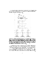
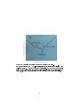
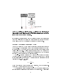
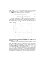
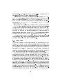
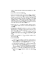
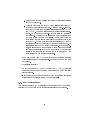
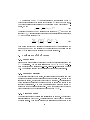
Research Internship
at University of Toronto
under Prof. Joseph H. Thywissen
on the project
Frequency Modulation Saturation
Spectroscopy Laser Lock of An
Interference-Filter-Stabilized
External-Cavity Diode Laser
Felix Stubenrauch
September 16, 2010
Abstract
This document gives a short theoretical introduction to Frequency Modulation Saturation Laser Lock. Moreover, the experimental realization of a
lock for an external-cavity diode laser is described and characterized and a
short manual of how to start the laser lock setup and to optimize the error
signal is given. It continues the work of Matthias Scholl which is described
in [1].
1
Contents
1.
2.
3.
4.
5.
6.
Motivation (Summary) . . . . . . . . . . . .
Theory . . . . . . . . . . . . . . . . . . . . .
2.1. Saturation Absorption Spectroscopy
2.2. Laser Lock . . . . . . . . . . . . . .
Experiment, Setup . . . . . . . . . . . . . .
3.1. Optical Isolator . . . . . . . . . . . .
3.2. Electro-optical Modulator (EOM) . .
3.3. Vapor Cell . . . . . . . . . . . . . . .
3.4. Photo Diode . . . . . . . . . . . . .
3.5. Getting started . . . . . . . . . . . .
3.6. Beat Measurement . . . . . . . . . .
Perfomance of the System . . . . . . . . . .
4.1. Error Signal . . . . . . . . . . . . . .
4.2. Frequency Stability . . . . . . . . . .
4.3. Recapture Range . . . . . . . . . . .
4.4. Long-time drift . . . . . . . . . . . .
4.5. Linewidth And Noise . . . . . . . . .
4.6. Sidebands . . . . . . . . . . . . . . .
What could be improved? . . . . . . . . . .
Conclusion . . . . . . . . . . . . . . . . . . .
2
.
.
.
.
.
.
.
.
.
.
.
.
.
.
.
.
.
.
.
.
.
.
.
.
.
.
.
.
.
.
.
.
.
.
.
.
.
.
.
.
.
.
.
.
.
.
.
.
.
.
.
.
.
.
.
.
.
.
.
.
.
.
.
.
.
.
.
.
.
.
.
.
.
.
.
.
.
.
.
.
.
.
.
.
.
.
.
.
.
.
.
.
.
.
.
.
.
.
.
.
.
.
.
.
.
.
.
.
.
.
.
.
.
.
.
.
.
.
.
.
.
.
.
.
.
.
.
.
.
.
.
.
.
.
.
.
.
.
.
.
.
.
.
.
.
.
.
.
.
.
.
.
.
.
.
.
.
.
.
.
.
.
.
.
.
.
.
.
.
.
.
.
.
.
.
.
.
.
.
.
.
.
.
.
.
.
.
.
.
.
.
.
.
.
.
.
.
.
.
.
3
3
3
5
11
11
11
13
14
14
16
18
18
18
18
19
20
22
22
23
1.
Motivation (Summary)
Many labs all over the world are working with Ultra Cold Atoms to study the
quantum behaviour of atoms and molecules and to test or improve theoretical
models that are important to understand popular and interesting phenomena
like high temperature superconductivity or how to build a quantum computer
that could have a great impact on how we live in the future. In the Ultra
Cold Atoms lab at University of Toronto atoms are loaded into a lattice
potential with tunable interactions between the atoms to simulate atoms in
condensed matter system and to test and study the Hubbard model that
exactly describes this system but is not solvable analytically.
One major step of bringing the atoms to these very low temperatures is
laser cooling, that was simultaneously proposed by Wineland and Dehmelt
[2] as well as Hänsch and Schawlow [3], which is still used widely to cool
the atoms to temperatures about 100 µK . To reach temperatures that are
needed to create BECs or degenerate Fermi gases and that are about two
magnitudes of order lower evaporative cooling is used.
The lasers that are used in laser cooling need high frequency stability and
small linewidth (< 1 M Hz ). Several techniques are established to stabilize
lasers to fulll these requirements. This report describes the realization
and characterization of a Frequency Modulation Spectroscopy laser lock. It
concentrates on the creation and the optimization of the error signal and
doesn't talk about the control servo needed to create the signal that is fed
back to the laser. At the time when this report was written the laser were
only locked with slow piezo feedback. However, the performance has already
been sucient to be used in the experiment but will be further improved by
using fast current feeback.
2.
2.1.
Theory
Saturation Absorption Spectroscopy
One of the major applications of lasers is the investigation of the energy
structure of atoms and molecules with laser spectroscopy. With a single laser
it is possible to reach resolutions that are only limited by the Doppler-width
of the atomic transitions as long as the laser linewidth is smaller than the
Doppler-width. Our laser has a free running linewidth of ∆νf ree ≈ 1 M Hz
which is much smaller than the ∆νdoppler ≈ 1, 25GHz Doppler-width of the
Potassium D2-line at 766, 7 nm [4] that is used as an atomic reference in our
setup.
3
However, it is possible to resolve energy levels within the Doppler-broadening
if the atomic vapor is saturated by a so called pump laser as it is the case in
saturation absorption spectroscopy (1).
Figure 1: A saturated absorption spectroscopy (SAS) experiment [5]. a) Basic SAS
setup. b) Shape of photo diode signal without and with pump beam. c) Velocity
(only component in beam direction) distribution of atoms in a two level system with
increasing beam frequencies from left to right hitting the resonance on the picture in
the center. Positive velocities are dened in probe beam direction. The thick arrows
are pointing out the higher intensity of the pump beam.
The picture on the bottom of gure 1 shows the velocity distribution of
the atoms in the ground and the excited state. If the beam with frequency
f is for example red-detuned from resonance at f0 to lower frequencies by
δ = f −f0 , atoms have to counterpropagate the beam with a velocity v = fδ0 ·c
to get a doppler-shift that brings them back to resonance. Only atoms
with a velocity in a narrow interval around this velocity will be excited.
4
Therefore, atoms that are resonant with the probe beam (thin arrow) have
negative velocities (because positive velocities are dened in probe beam
direction). Since probe and pump have the exact same frequency, atoms that
are resonant with the pump beam must have the same value but opposite
sign of velocity. Both, pump and probe beam excite resonant atoms from the
ground into the excited state leaving "`holes"' in the velocity distribution of
the ground state.
When the laser beam is in resonance with the atomic transition δ = 0,
both, pump and probe beam get resonant with atoms that have velocity components in beam direction that are close to zero. The deep hole "`burned"'
by the pump beam reduces the number of atoms available for excitation
through the probe beam and therefore reduces the absorption of the latter.
This results in the sub-doppler resolution peak at resonance shown in inset
b). So far, we only looked at simple two level systems. In systems with more
energy levels additional peaks (crossover peak) appear exactly halfways between the resonance of two transitions in the SAS signal due to hole burning
and optical pumping [6], [7].
Figure 2 shows the 39 K D2-line signal with F = 1, F = 2 and crossover
peak (see potassium energy level structure showing the D1 and D2-line in
gure 3).
2.2.
Laser Lock
As mentioned before, our homebuilt ECDLaser system has to work at a very
stable frequency (±1 M Hz ) with a narrow frequency distribution. There
are several techniques to "`lock"' (stabilize) a laser to a certain frequency
that ensure this. Single beam methods like dichroic atomic vapour laser
lock (DAVLL) have doppler-broadened features which results in large recapture ranges of several hundred MHz. However, the sub-doppler resolution of
saturation spectroscopy methods like frequency modulation saturation spectroscopy (FMS), which is applied in this project, leads to steeper gradients
of the error signal ensuring higher stability. Moreover, the atomic vapor that
is used in FMS gives an absolute frequency reference.
Error Signal
The underlying principle of all lock-in methods is to create a so called error
signal that is proportional to the dierence between the actual, possibly
perturbed frequency of the laser and the reference frequency that is often
obtained by using an atomic transition (see g. 4, more details in the follow5
Figure 2: Saturation absorption spectroscopy signal of our setup. F = 1, F = 2
and crossover peaks of the 39 K D2-line are labeled (see potassium energy levels D1 and
D2-line in gure 3. 41 K isotope peaks are barely visible. We dont substract the single
beam doppler peak because it doesn't contribute signicantly to the error signal (see
section 2.2.) (which is proportional to the rst derivative of the saturation signal).
6
Figure 3: Energy level structure showing the D1- and D2-line of the potassium
isotopes 39 K, 40 K and 41 K from [4].
7
Figure 4: Principle of a laser lock setup. A small part of the laser intensity is
used to create an optical frequency dependend signal that is detected and manipulated
electronically to create a linear frequency depend error signal that is fed back to the
laser to correct for the frequency aberration.
ing sections). This signal is fed back to the laser to correct the aberration for
example by changing the voltage of a piezo crystal that changes the length
of the laser cavity or by controlling the current of the laser diode.
Frequency Modulation Spectroscopy (FMS)
As in SAS a strong pump beam is used to saturate the excitation of atoms in
a vapor cell. The transmission of the weak counterpropagating probe beam
is detected. In FMS however, the probe beam frequency is modulated before
passing the vapor cell. The error signal is extracted from the magnitude of
the frequency component of the signal that oszillates with the modulation
frequency. This is described in the following section.
An Electro-Optical Modulator (EOM) is used to modulate the phase of
the probe beam. The phase shift of light Φ on the output of the EOM crystal
is proportional to the electric eld Ea applied inside the birefringent crystal
(see also Pockels-eect, e.g. [8]):
Φ=
βω0
Ea l,
c
(1)
where l is the length of the crystal in beam direction, β is the Pockels coefcient and ω0 is the frequency of the beam.
The polarization of light travelling through the crystal stays linear if the
light is polarized parallel or perpendicular to the optical axis. A periodically
8
varied voltage V = V0 sin(ωm t) is applied over the height d of the crystal
with modulation frequency ωm creating a maximal phase shift of Φmax =
M = βωc 0 dl V0 . The modulated light can than be written as
E(t) = E0 exp[i(ω0 t + M sin wm t)]
= E0 exp(iω0 t)
+∞
X
Jn (M ) exp(inωm t).
(2)
(3)
n=−∞
The phase modulated light may also be written as the Fourier sum of
equally spaced xed frequencies with amplitudes that are given by the nth
order Bessel functions Jn as in 3. The rst three order Bessel functions are
shown in gure 5.
Figure 5: First three order Bessel functions. Vertical line shows modulation depth in
our setup at M ≈ 0.7(rad).
The following mathematical derivation is taken from Hall's and North's
review (2000) [9]. The eect of a sample of length L with an absorption
coecient α(ω) and index of refraction η(ω) can be written in terms of a
complex, frequency-dependent transmission function, T (ω) = exp(−δ − iψ),
with amplitude attenuation δ and phase shift ψ , where δ(ω) = α(ω)L/2 and
ψ(ω) = η(ω)Lω/c. The frequency dependence of δ is the absorption line
shape, and the frequency dependence of φ is the dispersion line shape. The
electric eld transmitted through a sample then depends on the absorption
and dispersion at the carrier frequency and all the sidebands according to
9
E(t) = E0 exp(iω0 t)
+∞
X
T (ωn )Jn (M ) exp(inωm t).
(4)
n=−∞
The even and odd order sidebands are, respectively, in and out of phase,
as the Bessel functions of negative integer order have the symmetry property
J−n (M ) = (−1)Jn (M ). Therefore the amplitude modulations caused by two
symmetric sidebands are out of phase and exactly cancel out leaving pure
frequency modulation. Because of the frequency dependence of the attenuation, however, the sidebands have dierent amplitudes after the transmission
through the probe leading to amplitude modulation at the modulation frequency ωm that is linear in the dierence of the attenuation of the two rst
order sidebands (gure 6).
Figure 6: The three upper graphs show the sideband attenuation for dierent frequencies of the main peak with the corresponding DC-error-signal underneath.
A DC error-signal that is proportional to the amplitude modulation depth
may be extracted by mixing the detected signal with the modulation signal. This signal has to be low pass ltered below the modulation frequency
because it contains contributions of integer multiples of the modulation frequency. In the limit of weak modulation M < 1 only the rst order sidebands
contribute to this signal leading to an intensity
IF M = E0 exp(−2δ0 )[M (δ−1 − δ+1 ) cos θ + M (ψ−1 + ψ+1 − 2ψ0 ) sin θ], (5)
where δi and ψi are the attenuation and the dispersion of the ith order
sidebands and θ is the phase shift between the modulation signal and the
saturation signal in the mixer. The dispersion term can usually be neglected.
10
Especially for a symmetric dispersion prole around the resonance frequency.
Equation 5 shows that we have to match the phase θ, improve the absorption
signal or increase the modualtion amplitude M to get a strong error signal.
The treatment using xed frequencies only makes sense when the frequency is modulated fast in the timescale of absorption ωm & Γ, where Γ
is the linewidth of the transition. For slow modulation the time-dependent
transmitted intensity just follows the absorption spectrum at the instantaneous frequency, without a phase lag. The natural linewidth of the 39 K
D2-line is about 6 M Hz which is broadened in the saturation spectroscopy
signal because of insucient resolution to resolve transitions to dierent hyperne states in the excited 2 P3/2 -level and because of power broadening.
For very high modulation frequencies the sidebands showed in gure 6 lie far
away from the absorption peak and the dierence between them and hence
the error signal stay small. The optimal modulation frequencies for our setup
therefore lie between 10 M Hz and 35 M Hz .
3.
Experiment, Setup
Figure 7 shows our realization of the Frequency Modulation Saturation Spectroscopy Laser Lock. In the following paragraphs it will be explained how to
start the laser setup in practice and how to get the optimized error signal.
3.1.
Optical Isolator
The alignment of the optical isolator should be done as described in the
user's manual.
3.2.
Electro-optical Modulator (EOM)
We have chosen a commercial broadband electro-optic phase modulator EOPM-NR-C1 from Thorlabs to be able to tune the modulation frequency to
optimize the phase between the photo diode signal and the modulation signal in the mixer. Resonant mode modulators have the advantage of higher
modulation depth M when used with a tank circuit. The modulation signal
for the broadband EOM in our setup, however, has to be amplied by a 2 W
amplier (minicircuits, ZHL-1-2W). Because of the poor impedance matching most of the power is reected back from the crystal into the amplier
which has to be cooled by an additional fan over the pre-mounted heat sink.
We also considered attenuating the amplied signal before the EOM because
the reected power would be attenuated another time before reaching the
11
Figure 7: Laser Lock Setup. For reasons of simplicity most mirrors that are necessary
for beam alignment are not shown in this schematic. Electronics from minicircuits are
shown with part numbers.
12
amplier again. However, this reduced the peak-to-peak amplitude and the
signal-to-noise ration of the error signal signicantly.
With this setup we achieve modulation amplitudes of around V0 = 40 V .
The EOM has a half-wave voltage (voltage that has to be applied to create a 180 degree phase shift) at 767 nm of 173 V leading to M ≈ 0.7. As
shown in gure 5 the second order sideband is still negligible with a relativ intensity of [J2 (0.7)/J0 (0.7)]2 = 0.4 %, where as [J0 (0.7)]2 = 75.9 % and
[J1 (0.7)/J0 (0.7)]2 = 15.3 %.
!! Make sure that you start the amplier with low modulation powers of
< −30 dBm before turning up to avoid high peak power in the amplier!! If
you are not sure if the function generator is turned down to low powers from
the previous run, switch o the amplier by unplugging the 24 V bananas
and check the power on the function generator) The power input for the
amplier should always stay under 10 dBm. The amplier starts getting
non linear for power input (1 dB Compr., see datasheet) over 4 dBm.
The beam through the EOM should be aligned by increasing the transmitted intensity rst. When the error signal is obtained the alignment may
be further improved by optimizing the error signal.
3.3.
Vapor Cell
We heat the potassium vapor cell to increase the absorption rate with a
current of 2 A through a thin wire that is coiled around the cell on both
ends but not in the middle. Thus the potassium atoms do not condense on
the outer surfaces (but in the colder middle) of the cell which would lead to
reections of the beams. The current of two adjacent heating wires is always
running in opposite directions to avoid strong magnetic elds. A fan on top
of the power supply which produces a lot of heat is used for cooling.
We rst tried to align the two counterpropagating beams through the
vapor cell on top of each other and separating them with a polarizing beam
splitter (PBS) reecting the probe beam into the photo diode. This means
that probe and pump must have perpendicular polarization in the cell which
is no problem as long as there is no magnetic elds that lead to Zeemansplitting of the absorption lines. However, the magnetic elds created by
the heating wires of the vapor cell are strong enough to distort the error
signal due to the splitting (even though the current of two adjacent heating
wires is always running in opposite directions). Therefore, we switched to
the alignment that is shown in the schematic using a λ/2-waveplate to get
parallel polarization for pump and probe beam. The beams lie in one horizontal plane crossing each other in the middle of the vapor cell and having
13
a horizontal distance of ≈ 5 mm on the vertical input and output surfaces
of the cell.
3.4.
Photo Diode
In the current setup a PDA8A photo diode from Thorlabs is used. It has a
xed gain and a large bandwith from DC to 50 M Hz . The detected and DCblocked (since only the modulated components of the signal contribute to the
error signal) signal has to be amplied by an external amplier (minicircuits,
ZLN-500BN-LN). To decrease the noise produced by the amplier and the
mixer an attenuator is used in front of the amplier leading to a smaller
peak-to-peak error signal. A good trade-o leading to an optimized ratio of
signal to noise could be achieved by using a 6 dBm-attenuator (minicircuits,
HAT-6+).
We previously used the slower PDA36A photo diode from Thorlabs with
adjustable gain. Since the bandwith of 17 M Hz (0 dB gain, 12, 5 M Hz for
10 dB gain) was only about enough for no gain two external ampliers had
to be used leading to higher noise.
3.5.
Getting started
In this section it is described how to start both lasers. The list refers to the
setup when the two EOMs are driven by a single frequency modulator (SRS
model DS345) with double tee output (modulation signal for both mixers and
signal piezo ramp) and amplied by a single amplier (minicircuits, ZHL-12W) with a power splitter (minicircuits, ZX10-12-2) at the output. Moreover
the oszilloscope only shows the error signal. If you can't generate an error
signal following this list, you should try to get the saturation signal rst.
Probably the electronics don't work correctly, the photo diode is saturated,
the phase between the saturation signal and the modulation signal at the
mixer might be wrong, the alignment is bad or the vapor cell isn't heated
up enough. Moreover the saturation signal is easier to nd because of the
broad doppler peak that is suppressed in the error signal.
• Switch on the power suppliy that heats the vapor cells. Make sure that
it runs at around 2.0 A or 5.8 V . Fan will be turned on with ramp/lock
box.
• Switch on laser to around 70 mA. All temperature controls should show
values between 10 kΩ and 15 kΩ. Make sure the beam isn't blocked.
14
Wait 10 minutes until cell temperature reaches equilibrium and laser
stabilizes.
• Switch on photo diodes and oscilloscope.
• Switch on power supply for lock box, fans and ampliers. Unplug and
replug the 24 V bananas to start fan. Make sure all fans are running.
• Turn ramp on/lock o and ramp up to maximum. Start piezo mod-
ulation function generator. Center piezo bias on lock box and piezo
controller to around 70 V to get maximum tuning range. (Check bias
tuning range on lock box by turning it all the way up and down and
watch the voltage on the piezo controller. Change bias to the middle
of the tuning range and turn piezo controller to 70 V
• Start and turn up EOM modulation on function generator to around
0 dBm. (!!! read section about EOM rst to avoid destroying the
amplier!!!)
• Tune laser diode current slowly between 60 mA and 100 mA until a
signal appears on the scope. Make sure the scope diplays the whole
piezo tuning range. You expect a signal with 20 to 200 mV on the
scope. Center signal around t = 0 s with piezo controller. This procedure sometimes requires a bit of patience. If you loose the mode, try
again.
• Turn up EOM modulation to 5 dBm. This should be enough to see
strong error signals.
• Optimize error signal:
Change pump-probe relation by turning the waveplate before the
second polarizing beam splitter (PBS). Make sure you stay in the
limit of a strong pump beam realizing at least Ipump > Iprobe .
Change intensity in saturation arm by turning waveplate before
the rst PBS. Use beam intensities close to Ipump ≈ 350 mW
and Iprobe ≈ 50 mW to avoid power broadening of the saturation
peaks and saturation of photo diode, signal amplier or mixer.
Realign EOM by optimizing the error signal (Just look if you can
increase the peak-to-peak signal by changing the mirror orientation).
15
Change probe and pump alignment through vapor cell and realign
probe to photo diode.
Optimize phase between the two mixed signals (see theory) by
changing the modulation frequency. Maximum peak-to-peak signal should be found for modulation frequencies between 10 M Hz
and 30 M Hz . For some frequencies the noise decreases signicantly. Try to nd a good trade-o between noise and amplitude
of the signal. The slope of the linear area of the transition that
you want to lock to has to be positive! You can also change the
cable length to optimize the phase since the wavelength is in the
order of 10 m. This is more eort and less elegant but would be
necessary if a cheap xed frequency modulator would be used. An
alternative would be a homebuilt phase shifter. If you unplug cables, always switch o the ampliers to avoid high peak currents
and power reections! If both EOMs are driven by one function
generator the phase for one of them has to be optimized by the
cable length or a homebuilt phase shifter.
• Ramp down to see only F = 2 peak (see gure 2) until ramp sweeps
over the linear area of the error signal. Switch o the ramp and turn
on the lock.
• The laser is locked! =)
• To see beat signal AOM has to be turned on (−5 dBm at function
generator) because only the shifted rst order beam of the left laser
setup is coupled.
• !! If you shut down the setup always shut down the function generators
continiously and before switching o the ampliers!!
3.6.
Beat Measurement
This section describes how to interpret the beat signal on the spectrum
analyzer (SA) of two beams with dierent frequencies and amplitudes .
16
Linewidth
If we treat the random frequency distribution caused by random noise as a
gauÿian distributed error
s
σbeat =
σ1
2
∂ωbeat
∂ω1
2
+ σ2
2
∂ωbeat
∂ω2
2
,
(6)
where σbeat , σ1 and σ2 are the standard deviations of the frequencies ωbeat =
ω1 − ω2 , ω1 and ω2 , we get
∆ωbeat =
p
∆ω1 2 + ∆ω1 2
(7)
because σ ∝ ∆ω1 has no correlation with ∆ω2 . If one knows the linewidth of
one laser or a relation between the linewidth of both lasers, one can calculate
the linewidth of the other laser from the linewidth of the beat signal.
Intensity
The intensity I beat of the beat signal can easily be derived from
I beat = |E1 (t) + E2 (t)|2 = |A cos(ω1 t) + |b cos(ω2 t)|2
1
= [2A2 cos(2ω1 t) + 2B 2 cos(2ω2 t)
4
+ 4AB(cos((ω1 + ω2 )t) + cos((ω1 − ω2 )t))]
(8)
f ilter
→ AB cos((ω1 − ω2 )t).
The low pass ltered detected intensity at the frequency ω1 − ω2 is therefore
proportional to the product of the amplitudes AB of the electromagnetic
elds of the two beams that are superimposed.
Sidebands
The intensity of the main peak is I0beat ∝ A0 B0 , with A0 and B0 being the
amplitudes of the Fourier components of the main frequency ω01 and ω02 of
the two beams. We assume that the second beam has rst order sidebands
with eld amplitudes B±1 . For the intensity of the beat signal of the rst
beat of the second beam and the main frequency of the rst
order sidebands I±1
beam with eld amplitude A0 we get
beat
I±1
= cA0 B±1 = I0beat
17
B±1
B0
(9)
The signal on the SA SSA is proportional to the electronic power Pel
which is proportional to the square of the voltage VP D from the photo diode.
The voltage itself is proportional to the intensity of the beat signal I beat .
Hence, we get
p
p
SSA ∝ Pel ∝ VP D ∝ I beat .
(10)
side and the main
Therefore the ratio of the SA signals of the sidebands SSA
main is proportional to the ratio of the intensities of the sidebands
frequency SSA
I±1 and the main frequency I0 :
side
SSA
∝
main
SSA
beat
I±1
I0beat
!2
=
B±1
B0
2
=
I±1
I0
(11)
This means that if the SA signal of the sidebands is 40 dB smaller than the
main peak on the SA the intensity of the sidebands in the experiment are
also 40 dB smaller than the intensity of the main frequency.
4.
4.1.
Perfomance of the System
Error Signal
Figure 8 shows exemplarily the frequency dependend error signal around the
F = 2 transition. We get error signals with 600 mV to 800 mV peak-topeak amplitudes and signal(peak-to-peak-voltage)-to-noise ratios of about
100. The noise is measured in the horizontal parts of the error signal.
4.2.
Frequency Stability
The frequency stability of the (piezo, int) locked laser was measured in a beat
measurement against a locked laser from another experiment. As long as the
laser stayed locked, no frequency drift could be observed. The resolution of
this measurement is limited because it is hard to locate the center of the
frequency distribution. The peak has several local maximums caused by
noise that change position continuously. As an upper limit for the drift we
take the linewidth of the beat signal which is about 1 M Hz .
4.3.
Recapture Range
The recapture range of the laser lock is illustrated in gure 9. The frequency
scale is calibrated with the SA. The laser frequency was detuned by changing
the piezo voltage. Than the time shift of the error signal was compared to the
18
Figure 8: Error signal of the F = 2 transition.
frequency shift on the SA. This calibration has to be done each time because
it depends on the sweep voltage. The large recapture range of 227 M Hz
can hardly be realized since the error signal is slightly shifted horizontally
over time leading to zero crossings between the peaks. Therefore the factual
recapture range is about 70 M Hz . The servo is usually fast enough to correct
the laser frequency before it changes its frequency more than this.
4.4.
Long-time drift
It is important to consider long-time drifts as a property of the laser when
talking about a laser lock because it leads to losing the lock when the drifts
get to large.
The frequency of the unlocked laser drifts over time due to temperature
changes and other inuences, even though the temperature is controlled close
to the photo diode and on the bottom of the aluminium housing. Since these
drifts are very slow on a timescale of minutes or hours as shown in gure 10 it
is easy for the integrator in the servo loop to compensate them by changing
the piezo voltage over time. However, the servo can only change the piezo
voltage over ±25 V (if bias on servo box is perfectly centered). Because
of the frequency tunability of the piezos ((−53 ± 2) M Hz/V and (−41 ±
2) M Hz/V ) the servo can compensate for long-time drifts in frequency of
maximal ±1.3 GHz and ±1.0 GHz respectively. Therefore, the lock only
19
Figure 9: Frequency depend error signal with frequency scale. The frequencies refer
to the distance between the tips of the arrows. The two peaks correspond to the F = 2
transition (left) and the crossover (right) between F = 1 and F = 2
works for several hours (the laser has never been seen to stay locked for
more than 12 hours [over night]). The time can be extended if the piezo
voltage controller is used to decrease the servo feedback voltage from time
to time which can be realized by looking at the servo output voltage on a
additional scope. The piezo controller has a tuning range from 0 to 140 V
which makes it possible to lock theoretically over maximal frequency drifts
of ±3.7 GHz for the left setup (R = 22% or laser 3 in [1]) or ±2.9 GHz for
the right setup (R = 17% or laser 4 in [1]).
4.5.
Linewidth And Noise
To isolate the laser cavities from acoustic noise from the table, the lasers are
mounted on absorbing rubber (sorbothane). The bolts that are connected
to the table don't touch the cavity, either. They only touch the rubber.
We had to wait several days until the output beam of the lasers stayed
aligned. Therefore, you should not put to much weight on the laser cavities
and squeeze the rubber because it could take time until the alignment stays
stable again.
The cover for the cavity that protects the inside from air ows is also
acoustically isolated through rubber on top of the cavity.
20
Figure 10: An exemplary measurement of the frequency drift of the unlocked laser 3
with the spectrum analyzer in a beat measurement against a locked laser from another
experiment.
21
This and the strong error signal make the lock stable against metallic
objects hitting the table, like a falling pedestal. Even hitting the table with
a screw driver next to the laser doesn't unlock the laser.
After applying the rubber to the cavity, the noise measurement that is
described in [1] was repeated on the linear slope of the error signal. No peaks
could be found but only at white noise.
The linewidth was measured by translating the noise of the error signal of the piezo feedback locked laser to frequency uctuations, leading to a
linewidth around 1 M Hz with 30 % high errors. This measurement overestimates the linewidth, however, because we took the maximum error signal
uctuations on the scope to calculate the frequency uctuations. Measurements with the SA lead to similar results (using ∆ω1 = √12 ∆ωbeat for two
beams with same linewidth ∆ω1 ). Since the piezo feedback is very slow in the
order of ≈ 1 kHz the lock without current feedback doesn't have any measurable inuence on the linewidth of the laser compared to the case where
it is free running.
However, it will be interesting to measure the linewidth of the current
locked laser.
4.6.
Sidebands
Since we spent a lot of thoughts on sidebands caused by longitudinal external
cavity modes, this short section is talking about them.
The free spectral range of the external cavity is 1.7 GHz as shown and
explained in [1]. In the beginning, these sidebands showed up on the beat
signals between our two ECDLs with minimal relativ intensities from 30 dB .
Minimal means that they where sometimes even bigger depending on the
laser diode currents. Also Matthias Scholl already observed them. Even
after several internal alignments of the lenses and the interference lter they
could only be decreased to relative intensities of 40 dB . After rearranging
the setups on the optical table and reoptimizing the lasers the sidebands
dissappeared from the SA signal. This means that they have smaller relative
intensities than 50 dB now.
5.
What could be improved?
• Get power splitter after EOM amplier with higher max. power input.
• Built xed frequency modulator for sweep and EOM modulation and
phase shifter to optimize error signals independendly.
22
• Measure linewidth and short time stability when lasers are locked with
fast current feedback and piezo feedback to correct slower frequency
drifts.
6.
Conclusion
We have been able to build an interference-lter-stabilized external-cavity
laser in the lab and lock it to the 3 9K D2-line transitions via frequency
modulation spectroscpy. Even with a slow integrator feedback to the piezo
we achieve favorable linewidth and frequency stability of less than 1 M Hz .
The error signal and the isolation of the cavity from the optical table using
rubber pads are good enough to keep the laser locked even when people
are moving metallic objects over the optical table. The laser normally stays
locked over several hours. If the current error signal is used with a fast current
feedback a signicant improvement in linewidth and short time stability is
expected. The laser is ready to be used in cold atoms experiments in the
lab!
23
Bibliography
[1] M. Scholl and J. H. Thywissen. Interference Filter Stabilized External
Cavity Diode Laser. Ultra Cold Atoms Lab, Department of Physics,
University of Toronto, Canada, 2010.
[2] D. Wineland and H. Dehmelt.
, 20:637, 1975.
Bull. Am. Phys. Soc.
[3] T. W. Hänsch and A. L. Schawlow. Optics Communications, 13:68, 1975.
[4] T. G. Tiecke. Properties of Potassium. Diploma thesis, van der WaalsZeeman institute, University of Amsterdam, 2010.
[5] C. J. Foot.
. Oxford University Press, New York, 2005.
Atomic Physics
[6] W. Demtroeder.
Heidelberg, 2007.
. 5th ed., Springer-Verlag, Berlin,
Laser Spectroscopy
[7] University of Florida. Saturated Absorption Spectroscopy. Department of
Physics, Advanced Physics Laboratory, PHY4803L.
[8] P. W. Milonni and J. H. Eberly.
[9] G. E. Hall and S. W. North.
Lasers
. Wiley, New York, 1988.
Annu. Rev. Phys. Chem.
24
, 51:243, 2000.