Download Casio FX-8700G Owner`s manual

A
L
C
C
U
G
LATORS
N
I
H
P
A
R
G
IN THE SCIENCE CLASSROOM
GLENCOE
McGraw-Hill
New York, New York
Columbus, Ohio
Woodland Hills, California
Peoria, Illinois
Technology Consultants
Christine A. Lucas
Mathematics Teacher
Whitefish Bay High School
Whitefish Bay, Wisconsin
Jill Baumer-Piña
Former Program Assistant
The Ohio State University
Columbus, Ohio
Other Titles in the Glencoe Science Professional Series
Alternate Assessment in the Science Classroom
Cooperative Learning in the Science Classroom
Performance Assessment in the Science Classroom
Copyright © 1999 by Glencoe/McGraw-Hill.
All rights reserved. Printed in the United States of America. Except as permitted under the
United States Copyrights Act of 1976, no part of this publication may be reproduced or
distributed in any form or by any means, or stored in a database or retrieval system, without
prior written permission of the publisher.
Send all inquiries to:
Glencoe/McGraw-Hill
936 Eastwind Drive
Westerville, OH 43081
ISBN: 0-02-825487-2
1 2 3 4 5 6 7 8 9 10
ii
045
05 04 02 01 00 99 98
GRAPHING
CALCULATORS
IN THE
SCIENCE
CLASSROOM
s
t
n
e
t
n
o
C
f
o
e
l
Tab
Introduction
An Introduction to Graphing Calculators ..............1
Using Graphing Calculators in Cooperative
Learning ..........................................................5
Graphing Calculators and the
Mathematics Curriculum .................................6
Graphing Calculator Capabilities ..........................7
Getting to Know Your Graphing
Calculator ........................................................8
Evaluating Mathematical Expressions............11
Applications
Solving Equations in One Variable......................34
Solving Quadratic Equations...............................35
Families of Graphs..............................................37
Maxima, Minima, and Zeros of Functions...........39
Solving Trigonometric Equations .........................41
Verifying Trigonometric Identities........................42
Solving Exponential and Logarithmic
Equations .......................................................43
Matrices
Entering Matrices ................................................44
Determinants, Inverses, and Operations..............46
Graphing Skills
Mode and Range ................................................12
Functions............................................................14
Trace and Zoom..................................................16
Systems of Equations...........................................19
Inequalities .........................................................21
Systems of Inequalities........................................23
Rational Functions ..............................................25
Radical Functions ...............................................27
Quadratic Relations ............................................28
Trigonometric Functions and Their
Inverses .........................................................30
Exponential and Logarithmic Functions ..............32
Statistics
Statistical Computations......................................48
Histograms .........................................................51
Scatter Plots and Lines of Regression...................54
Curve Fitting .......................................................56
Probability and Combinatorics ......................60
iii
Using Programs................................................62
Templates
Plotting Points in a Relation ................................63
Solving a System of Linear Equations ..................63
Using the Quadratic Formula..............................64
Using the Law of Cosines....................................65
Using Hero’s Formula .........................................65
Inner and Cross Products of Vectors ....................66
Sums of a Series..................................................67
Sums in Summation Notation .............................67
Graphical Iteration..............................................68
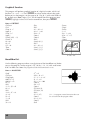
Mandelbrot Set ...................................................68
Generating Random Numbers ............................69
Evaluating a Function .........................................69
Area Between Two Curves ..................................70
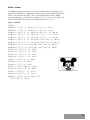
Mickey Mouse ....................................................71
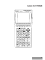
Casio fx-7700GE.................................................73
HP 38G ..............................................................74
Sharp EL-9200C..................................................75
TI-81...................................................................76
TI-82...................................................................77
TI-83...................................................................78
TI-92...................................................................79
iv
Appendix: Menus.............................................80
Index .................................................................82
GRAPHING
CALCULATORS
IN THE
SCIENCE
CLASSROOM
n
o
i
t
c
u
d
o
r
t
n
I
An raphing
to G lators
u
c
l
a
C
The graphing calculator offers you much more
flexibility in studying graphs than can be obtained
by paper and pencil graphing. Within seconds you
can graph an equation or a system of equations that
could take you several minutes to sketch. The
various functions on a graphing calculator can also
help you to analyze the graph in a way not possible
with traditional graphing techniques. For example,
when graphing an equation such as y x 4 3x 3 2x 2 x 10, no longer do you have to
spend time calculating the long list of ordered pairs
that give you points to sketch the curve. No longer
do you have to use the tedious repeated
calculations of the Location Principle to find the
zeros of the function. Instead, you can concentrate
on the attributes of the graph itself—For
what values of x is y increasing? Where does the
graph reach a maximum point or does it have
several maxima? Does the graph intersect the
x-axis? If so, how many times? How does the
behavior of the graph relate to the equation of the
graph? and so on.
It is important to understand that it is okay and
many times necessary to solve problems with a
calculator and that most of the time the calculator
does not “find the answer” but merely helps to find
appropriate solutions to problems. If you do not
understand how to interpret the information the
calculator provides, then it is of no use. It is still up
to you to make connections with the technology
and the mathematical concepts. The calculator
simply saves time and effort and allows you to go
deeper into mathematical concepts than you could
in the past. It also opens the door to solving
previously-unsolvable problems.
The calculator is not the solve-all instrument for
mathematical problems, but a tool for completing
the tedious tasks that used to take hours and lots of
paper to achieve before you could get to the real
meat of the problem. You should experiment with
the calculator to find applications that are
appropriate to the topic being studied.
The graphing calculator allows you to look at many
new areas of mathematics that until now were
restricted at certain levels because of their
difficulty. While it may take time to feel
comfortable with using graphing calculators and
you may be just beginning to learn how to use
them, it is important to keep trying and to keep
learning. Knowing when and how to use a graphing
calculator to solve problems will help you become
a better problem solver and that, of course, is the
ultimate goal.
In this guide to using graphing calculators in the
science classroom, you will encounter keystroke
instructions for graphing various types of equations,
as well as mathematical computations. Graphing
calculators are scientific calculators, as well as
hand-held computers, thus eliminating the need for
one calculator to graph and one to compute. There
are many manufacturers of graphing calculators
including Casio, Hewlett-Packard, Sharp, and Texas
Instruments. While all calculators share some
common characteristics, each differs in its
complexity and capabilities to graph various types
of functions.
In this guide, we will present keystrokes for Casio
and Texas Instruments calculators. The material in
this book is appropriate for both students and
teachers. Some of the procedures and keying
sequences found in this text may be helpful in
interpreting the instruction guides for other
calculators you may encounter.
To promote understanding of the sequencing of
keystrokes provided in this booklet, read through
the list of keystrokes first before entering them to
make sure you understand the purpose and
sequence. When solving a problem on your own
for the first time, it may be wise to write out the
keystrokes first before entering them into the
calculator.
1
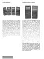
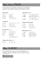
Casio Calculators
Hewlett Packard Calculators
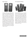
There are several different Casio graphing
calculators. There is also more than one model
available within each number series of calculator.
This guide includes keying sequences for the Casio
fx-7700GE calculator. It has a variety of capabilities
that permit you to perform calculations and
statistical analyses. It can graph equations in a
rectangular coordinate system, as well as graph
inequalities and parametric equations. In addition
to real number calculations, the fx-7700GE can
perform operations on matrices. The Casio fx8700G is a more advanced version of the fx7700G, appropriate for college-level mathematics
and engineering. Each calculator has programming
capabilities that you can study in detail by
consulting the owner's manual that comes with the
calculator.
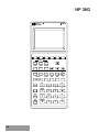
The Hewlett Packard family of graphing calculators
includes the HP 38G, HP 48G, and HP 48GX. All
of the Hewlett Packard models include pop-up
menus, input forms, and a built-in infrared
input/output port that lets you send and receive files
without using a cable. The input forms provide a
method to set up a problem by letting you fill in
blanks. The HP 38G stores a history of calculations,
allowing you to scroll back and copy a previous
input or result. It is capable of showing an
expression numerically, graphically, and
symbolically; and the split-screen feature lets you
choose which two screens you want to use for
comparison. The HP 38G includes matrix
operations and has the ability to graph polar
equations. It does not have the ability to graph
inequalities but it can shade and determine the area
of a region between a line or a curve and the x-axis
or another line or curve. The HP 38G is the only
calculator with ApLets. These are notes, pictures,
graphs, and custom-designed views combined into
an electronic lesson that allows you to explore a
problem. ApLets are available from Hewlett
Packard on floppy disk, at their Internet site, and on
their bulletin board. You can even create your own
ApLets. The HP 48G operates very similarly to the
HP 38G but has enhancements that include threedimensional graphics, and built-in equations. The
HP 48GX has four times more memory than the
other two models and has two expansion ports so
you can add more memory or customize it with
plug-in application cards.
2
Sharp Calculators
Texas Instruments Calculators
The Sharp EL-9200C and EL-9300C graphing
calculators have an equation editor feature that
allows you to enter an expression exactly the way it
appears in the textbook. Both models include
menus from which you can select specialized
modes. Matrix operations are included in the
calculation mode, while the graph mode lets you
graph functions using rectangular or parametric
coordinates. A unique feature in the graph mode is
the jump key. If you are in the rectangular
coordinate mode, this feature lets you jump to an
intersection point, minimum and maximum values,
and x- and y-intercepts. All the commands needed
in the program mode are in the menus or on the
keyboard. The statistics graph mode lets you graph
data entered in the statistics mode. There are six
kinds of data graphs and six kinds of regression
curves. The EL-9300C operates very similarly to the
EL-9200C but has enhanced features including a
communications port, four times as much memory,
and an equation solver function. The solver mode
provides three methods to solve for different
variables in equations.
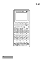
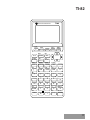
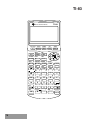
The Texas Instruments family of graphing
calculators includes the TI-80, TI-81, TI-82, TI-83,
TI-85, and TI-92. This guide includes sequences for
the TI-81, and TI-82/83 models. All of the Texas
Instruments models allow you to graph equations
and inequalities in a rectangular coordinate system,
as well as to graph parametric equations. The
higher the model number, the more sophisticated
the programming capabilities of the calculator.
These and the matrix feature of the TI-81 are
expanded in the TI-82/83 to include list operations,
sequences, tables, and more. The TI-85 has
additional features that are specially suited to
college-level mathematics and engineering. The
TI-92 has greatly expanded memory, and offers
symbolic manipulation, three-dimensional
graphing, and the ability to construct, measure, and
manipulate geometric figures.
3
GRAPHING
CALCULATORS
IN THE
SCIENCE
CLASSROOM
g
n
i
h
p
a
r
G
g
n
i
s
U ulators in
Calc erative
Coop ning
Lear
Cooperation is part of the real world at all levels,
whether it be among nations, with co-workers, with
neighbors, with your community, or within your
family. Individuals must develop skills and
understandings of working in groups to be
successful in today’s world.
The graphing calculator is a tool that will allow
students to work in groups, explore concepts, and
come to conclusions about the “rules” of
mathematics through their own understanding.
Research has shown that discovery and
internalization of this type is more deeply
understood than the dissemination of information
usually seen in a traditional lecture situation.
When students use a graphing calculator, they find
that they too have a powerful tool for asking
“What if...?” By encouraging students to explore
with the calculator, you open an unlimited world
of variety in viewing each function they graph.
For example, when graphing a line with graph
paper, they may anticipate the graph to look a
certain way. However, with the graphing calculator,
the appearance of the graph depends on the range
values used in the viewing window. By changing
the scale, students can make a graph appear more
or less steep than it is on traditional square grid
paper.
When students graph more than one function on a
viewing screen, they can explore how the two
graphs are related. For example, if two lines are
graphed, you could ask “Are the lines parallel or
not? How do you know? Could the lines be
perpendicular? How do you know? Do the lines
have any characteristics in common?” and so on.
The cooperative group becomes a field for
questioning and exploring. Emphasis is placed on
the discovery method. Because the calculator saves
time and is usually more accurate than studentdrawn sketches, the technical aspect of graphing
is set aside so that the real mathematics behind
the graph can be explored. That is, you are
enabled with the power to teach more
mathematics by removing the mechanical
manipulation time previously required with paper
and pencil.
In addition to graphing activities, the graphing
calculator lets students explore computational
patterns. When entering mathematical expressions
into the graphing calculator, unlike other scientific
calculators, the entire expression appears on the
screen as well as the final result. The REPLAY
feature on the calculator allows you to return to the
original expression and alter one or more parts of
the expression. In this way, students can explore
patterns in numbers that lead to a formula.
The expression “two heads are better than one”
seems appropriate when working in cooperative
groups. With a graphing calculator and a little
guidance, students can use their collective
resources to discover the same excitement about
mathematics and science that motivated the
mathematicians and scientists of the past to bring
us the concepts we study today.
You can learn more about using cooperative learning
techniques in Glencoe’s Cooperative Learning in the
Science Classroom, another booklet in the Glencoe
Science Professional Series.
5
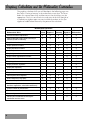
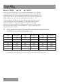
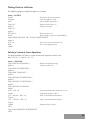
Graphing Calculators and the Mathematics Curriculum
The graphing calculator skills you will develop in the following pages can
be used in a variety of courses in the mathematics curriculum. The chart
below lists some of those skills and the course(s) for which they may be
appropriate. This list is not all inclusive, and many of the skills thought of
as second-year algebra topics are now available to students in first-year
algebra or middle school courses by the power of the calculator.
Mathematical Operations
Mathematical Skills
Evaluate numerical expressions
Perform operations with fractions resulting in
fractions (Casio fx-7700 only)
Graph linear functions
Graph quadratic functions
Middle
School
Algebra 1
Geometry
Algebra 2
Advanced
Mathematics
✓
✓
✓
✓
✓
✓
✓
✓
✓
✓
✓
✓
✓
✓
✓
✓
✓
✓
✓
✓
✓
✓
✓
✓
✓
✓
✓
✓
✓
✓
✓
✓
✓
✓
✓
✓
✓
✓
✓
✓
✓
✓
✓
✓
✓
✓
✓
✓
✓
✓
✓
✓
✓
✓
✓
✓
✓
✓
✓
✓
✓
✓
✓
✓
✓
✓
✓
✓
✓
✓
✓
✓
✓
✓
✓
✓
✓
✓
✓
✓
✓
✓
✓
✓
Graph polynomial functions
Graph inequalities
✓
Graph trigonometric functions
Graph inverse trigonometric functions
Graph exponential functions
Graph logarithmic functions
Graph parametric equations
Graph polar equations
Perform operations with matrices
Plot points
Connect points with segments
Draw histograms (bar graphs)
Graph scatter plots
Statistical computations (mean, standard
deviation, regressions, correlation coefficients)
Find the number of permutations
Find the number of combinations
Convert degrees to radians and vice versa
Convert polar coordinates to rectangular
coordinates and vice versa
6
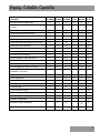
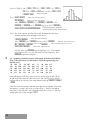
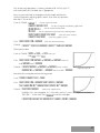
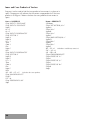
Graphing Calculator Capabilities
Capability
Casio
Sharp
fx-7700GE HP 38G EL-9200C
TI-81
TI-82/83
TI-92
✓
✓
✓
✓
✓
Evaluate numerical expressions
✓
✓
✓
Perform operations with fractions resulting in
fractions
✓
✓
✓
Graph linear and quadratic functions
✓
✓
✓
✓
✓
✓
✓
✓
✓
✓
✓
✓
✓
✓
✓
✓
✓
✓
✓
✓
✓
✓
✓
✓
✓
✓
✓
✓
✓
✓
✓
✓
✓
✓
✓
✓
✓
✓
✓
✓
✓
✓
✓
✓
✓
✓
✓
✓
✓
✓
✓
✓
✓
✓
✓
✓
✓
✓
✓
✓
✓
✓
✓
✓
✓
✓
✓
✓
✓
✓
✓
✓
✓
✓
✓
✓
✓
✓
✓
✓
✓
✓
✓
✓
✓
✓
✓
✓
✓
✓
✓
✓
✓
✓
✓
✓
✓
✓
✓
✓
✓
✓
✓
✓
✓
✓
✓
✓
✓
✓
✓
✓
✓
✓
✓
✓
Graph other polynomial functions
Graph inequalities
Graph trigonometric functions and inverses
Graph exponential and logarithmic functions
Graph parametric equations
Graph polar equations
Perform operations with matrices
Plot points, draw segments
Graph histograms and scatter plots
Perform statistical computations
Calculate combinations and permutations
Convert degrees to radians, vice versa
Convert polar coordinates to rectangular
coordinates, vice versa
Replay function
Linear Regression
Zooming in or out on image
Tracing to find the coordinates of a point
Programmable
Table of function values
✓
✓
✓
✓
Draw, measure, transform geometric figures
Three-dimensional drawing
Symbolic manipulation
Complex number calculations
✓
TI-83
Advanced calculus operations
✓
✓
NOTE: On pages 9–65, you will find keystroke instructions for specific mathematical skills. Below the title of
each section, you will find the four calculators listed above preceded by either an open circle () or
a closed circle (●). The open circle indicates that the calculator does not possess the capability for
that activity. A closed circle indicates that it does.
7
GRAPHING
CALCULATORS
IN THE
SCIENCE
CLASSROOM
o
t
g
n
i
Gett Your
Know ing
h
p
a
r
G lator
u
c
l
a
C
As with any new acquaintance, you need time to
get to know your graphing calculator. Before
beginning any specific task, look at the keyboard.
Think of something you are used to seeing on your
familiar scientific calculator and see if you can find
it on your graphing calculator. Before delving into
the manual, see if you can find a correlation to the
expressions written above the keys and how to
access them. Try to figure out what key is
equivalent to = on your old calculator. Try
various keys to see what happens. If you receive an
error message of some sort, turn the calculator off
and then on again. Questions will inevitably arise
that you need special help in answering. When that
happens, consult the calculator manual or a
colleague.
It is very important that students also get to know
the calculator. The first session you have with
graphing calculators in the classroom should be a
“play” period in which students explore the keys as
described above. Let students work in pairs sharing
a calculator. By working with a partner, students
can share ideas about which key does what, and if
they should get stuck, the problem-solving skills of
two people working together will often be enough
to overcome the difficulty.
8
In this section, we will explore some of the basic
functions of the calculator and how to access
menus on the Casio fx-7700GE and the TI
calculators. Greater detail on how to use the menus
for specific tasks are discussed later in this booklet.
How do I turn the calculator on?
Casio: Press å.
TI: Press O.
How do I turn the calculator off?
Casio: Press SØ (located above å).
TI: Press ‹Ø (located above O).
All calculators have an automatic turnoff feature to
prolong battery life. If the calculator is left on too
long without being used, it automatically shuts
itself off. If you press å on the Casio calculator,
the calculator will come on, but you lose whatever
was in the text screen. If you press O on a TI
calculator, it will come on with the same screen
image it had when it shut off.
How do I change the contrast so that I can see the
screen better?
Casio: …A and ¶ repeatedly (to darken) or
ª (to lighten).
TI: Press ‹ and hold down § to darken, or
press ‹ and hold down • to lighten. A
cursor appears in the upper right-hand corner
with a number from 1–9 to represent the
contrast. The higher the number, the darker the
screen. If you wish to change the contrast further
after the first adjustment, you must press ‹
again before using either arrow key again.
If you turn your calculator on and the screen is blank or
black, you may need to use the contrast adjustment to
achieve the correct viewing setting. If you must
increasingly darken your screen to read the display, it
may be time to change the batteries.
How do I use the functions written above the
keys?
Casio: Pressing S accesses the functions
printed in yellow above left of the key. Pressing
⁄ accesses the functions printed in red
above right of the key.
TI: Pressing ‹ accesses the functions printed
in blue above left of the key. Pressing ⁄
accesses functions printed in gray above right
of the key.
In the keystroke sequences in this booklet, these
functions are shown using the appropriate access key
and the function name rather than the actual key
pressed.
How do I clear what’s on the screen?
Casio: Press å to completely clear the displayed
formulas, numeric values, and texts. Use the Cls
(ClearScreen) function to clear graphs from
the screen. Press S∞e.
TI: Press Ç to completely clear the displayed
formulas, numeric values, or text. Clear graphs
by pressing YÇé for each line
that has an equation. To clear any images created
with the DRAW menu, press ‹P,
which accesses the DRAW menu. Then select
ClrDraw and press é.
How do I get out of a menu?
Casio: Pressing the É key returns you to the
home screen.
TI: The “QUIT” function lets you exit any menu.
On the TI-81, QUIT is accessed by pressing
‹Ç. On the TI-82/83, QUIT is
‹5.
Where do I find the = key on my calculator?
The graphing calculator is actually a small
computer. The = key is replaced by e
on Casio calculators and by é on TI
calculators.
How do I enter variables in an equation like
y x 2?
When graphing an equation like the one above, it
is not necessary to literally enter the letter Y and the
equals sign. The X is entered differently depending
on the calculator you have. For more information
on how to enter a function in order to graph it, see
pages 14–15.
Casio: D
TI-81: I
TI-82/83: ‹D
Likewise, you can move the cursor and use
D to remove any unnecessary information.
When I use the square root key, do I press the
function key before or after entering the number?
The graphing calculator, unlike some scientific
calculators, works like a mathematical sentence
writer. In fact, you see the sentence on the screen
as you create it. If you want to find 4
3
5
6, press
the keys in the order you would read it.
Casio: Press SR and then enter the
number, 4356. To calculate the result, press
e.
TI: Press ‹› to access the square root sign.
Then enter the number. To calculate, press
é.
Is the order of entering a trigonometric function
similar to the way we enter a square root sign?
The answer is yes. With many scientific calculators,
you must enter the angle being evaluated and then
press the appropriate key. With a graphing
calculator, you should enter the function first and
then the angle measure.
Is there a pi key on my calculator?
The answer is yes. On the Casio calculator, is
entered by pressing SF. On the TI
calculators, it is the second function of ^.
More information on how to access other function
keys is found in the instructions for the specific
mathematical skills for which they are used. See
Index on page 82.
Do I have to start over if I make a mistake in
entering an expression?
The answer is no. If you make a mistake while
entering the expression, you can use the left and
right arrow keys to go back through the expression
and correct your mistake. If the mistake is a wrong
number or operation, you can simply “type over”
the error with the correct number or operation. If
you left out something, move the cursor to the point
where you want to insert the information and use
the I key to insert the new information.
9
How do I know what’s on each menu?
The TI calculators and Casio fx-7700GE have many
functions that are accessed by using menus (lists of
options) and making selections. Sometimes you
may know what function you want to use, but you
have no idea where to find it. In the Appendix on
pages 80–81, you will find many of the menus that
are available on each calculator, how to access
them, and what each item on the menu means. In
future pages of this booklet, we will show the
actual keying sequence to access items in menus
which are used for specific mathematical tasks.
How do I use the TI menus?
Several keys on the TI calculators access menus.
These menus are discussed in greater detail as we
use them in this booklet. Page 81 also lists many of
the menus in greater detail.
Most of the menu keys actually access several
menus. Each of these is shown at the top of the
screen and can be accessed by using ¶ or ª to
highlight the menu you wish to use. The items in
each menu can be accessed by pressing the
number of the item or by using § or • to
highlight the item and then pressing é.
Many of the menus on the TI-81 and TI-82 are the
same. The TI-82 and TI-83 have more menus and
thus more features.
How do I use the menus on the Casio fx-7700G?
The menus on the Casio fx-7700G operate much
differently than those on TI calculators. Menus can
be accessed using second function keys. Selections
from menus are made by using the top row of keys
(F1 through F6).
10
For example, when you press S , six
rectangles appear at the bottom of the screen. Each
of these rectangles correspond to the F1 through F6
keys respectively. Not all menus have six
selections. When only four rectangles appear, then
these correspond to keys F1 through F4.
Regardless of how many rectangles appear, the
rectangles do not appear directly over the keys to
which they correspond. You must count which
rectangle you want to use and press the
corresponding F key. For example, if you want to
use the function defined in the fourth rectangle, F4
is the key you press to access that function.
All of the Casio functions are abbreviated by four or
less symbols. It may be helpful to make a list of
what each symbol represents until you become
familiar with the menus. Page 80 of the Appendix
gives further details on some of the more
commonly-used menu items and their functions.
Other menus appear in specialized modes, such as
SD for statistical data, REG for regression
calculations, and MATRIX for matrix entry and
operations. As with other menus, rectangles appear
at the bottom of the screen that correspond to the
F1 through F6 keys.
Evaluating Mathematical Expressions
●
Casio fx-7700GE
●
TI-81
●
TI-82/83
All graphing calculators observe the order of operations when evaluating a
mathematical expression. The calculators also have parentheses that are used in
the same way as in writing to group terms in an expression or to clarify the
meaning of the expression.
When you enter an expression in a graphing calculator, the entire expression
appears as you enter it. On TI calculators, the multiplication and division signs
do not appear as they do on the keys. Instead the calculator displays symbols
used in computer language. That is, * means multiplication, and / means division.
If you make a mistake, you can use the arrow keys to go back and correct your error
by typing over, by using the I (insert) key, or by using the D (delete) key.
1
2 32 (–6)(–8)
–4
Evaluate .
You must use parentheses to group the terms in the numerator.
Casio:
(2+3›-m6um8)/m4e
TI:
(2+3›-m6um8)/m4é
Note that the negative sign is
entered before the number
and that its key, m, is
different from the subtraction
key -.
The result is 9.25.
You can also use parentheses to denote multiplication. Thus, (–6)(–8) can be
entered that way on the calculator without using a multiplication symbol.
REPLAY
If you get an error message or discover that you entered the expression incorrectly,
you can use the REPLAY feature to correct your error and re-evaluate without
re-entering the expression.
Casio: Press j or k. The answer disappears and the cursor goes to the
beginning or end of the expression, respectively. Use the arrow keys
to move to the location of the correction. Then type over, use
S I, or use D to make the correction. Then press
e to evaluate. You do not have to move the cursor to the end.
TI:
On the TI-81 press §. On the TI-82/83, press ‹ E. The
expression is redisplayed below the previous evaluation with the
cursor at the end. Move the cursor using the arrows and make your
changes. Then press é to evaluate.
The REPLAY feature is very handy for evaluating polynomial expressions of
high degree, such as 4x4 5x3 3x2 45, for varying values of x.
2
Evaluate 3x 6 for x 3, 3, 4, and 6.
Evaluate the expression for x 3. Record the result. Use the REPLAY
feature to change 3 to 3. Evaluate again. Repeat changing 3 to 4, and
so on. If you use parentheses around the number representing x, it makes it
easier to find the place to substitute when using the REPLAY feature.
Example: 3 ( 3 ) - 6
11
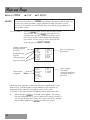
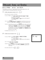
Mode and Range
●
●
Casio fx-7700GE
MODE
TI-81
●
TI-82/83
Each of the calculators has a 5 key. However, the type of mode and the way
in which you select the mode is slightly different for each calculator. In future
activities in this booklet, we will indicate when you need to change modes and
what mode(s) to use.
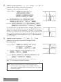
Casio fx-7000GE:
Pressing 5 once accesses the first menu screen
shown below. Pressing 5 again accesses the
second screen. To make a selection on either screen,
press the key of the number or operation preceding
your choice. You can also get to the second MODE
screen by pressing S 5.
Ordinary computation
graphing, program
execution
Writing/checking
programs
Clearing programs
Sys mode
1:RUN
2:WRT
3:PCL
[•:COMM]
REG model
4:LIN
5:LOG
6:EXP
7:PWR
Cal mode
:COMP
–:BASE-N
:SD
:REG
0:MATRIX
Contrast
:LIGHT
:DARK
Stat data
1:STO
2:NONStat graph
3:DRAW
4:NONDraw type
5:CONNECT
6:PLOT
Graph type
:REC
–:POL
:PARAM
:INEQ
Types of calculations to
be performed
Regression models
Statistical data
and graphs
Types of graphs
to be drawn
(equations/inequalities),
rectangular, polar, or
parametric
Notice the Draw type items at the lower left of the second screen. If you
select 6:PLOT, individual points whose coordinates the calculator has
computed will be shown on the graphing screen. If you select
5:CONNECT, then the calculator will plot the points and connect them.
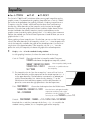
TI:
12
When you press 5, the mode screen appears. The settings
that are highlighted with a gray tint represent the setting currently in
use. You can change these settings by using the arrow keys to move
the tint block and pressing é to make your choice.
Normal
Sci Eng
Float 0123456789
Radian Degree
Func
Par
Pol
Seq
Connected Dot
Sequential Simul
FullScreen Split
Type of notation for display
Number of decimal places displayed
Type of angle measure
Type of graph
Whether to connect plotted points
How to plot selected functions
How to display results
Type of screen display
Normal
Sci
Eng
Float
0123456789
Radian
Degree
Func
Par
Pol
Seq
Connected
Dot
Sequential
Simul
Real
a+b i
re^i
Full
Horiz
G-T
TI-82
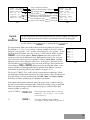
RANGE
or
WINDOW
TI-83
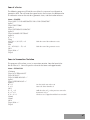
Use the range feature to set the parameters for the viewing window, including not
only the range for each axis but also the value of each tick mark on the graph.
On the TI-82/83, the fi key is replaced by the W key.
The range feature allows you to adjust how much of the graph you wish to view.
The notation [5, 5] by [6, 6] means a viewing window in which the values
along the x-axis go from 5 to 5 and the values along the y-axis go from 6 to 6.
For all of these calculators, the range is set in a similar manner. When you press
fi, a list of values appears. Xmin and Xmax mean the minimum and
maximum values on the horizontal scale. Xscl represents how many units you
wish each tick mark on the axis to represent. Likewise, Ymin, Ymax, and Yscl
represent similar values along the vertical axis. To change a value from the list,
use the arrow keys to scroll to the value you wish to change. Then type the new
value and press e or é. When you return to the graph screen, a new
viewing window will be displayed and your graph will be redrawn. For more
information on graphing and viewing windows, see pages 12–13.
WINDOW
Xmin =
Xmax =
Xscl =
Ymin =
Ymax =
Yscl =
Xres =
–5
5
1
–6
6
1
1
TI-83
The Casio fx-7700GE, TI-81, and TI-82/83 have parametric capabilities. When
you choose parametric mode and access the range function, you will find that the
list of parameters will also include entries for Tmin, Tmax, and Tstep (or Tptch).
Enter these numbers according to your problem’s parameters.
Each type of calculator has a default setting for range values. A default setting is
one that is built into the calculator and is used when no other setting is specified.
Many users prefer to begin with the default settings first and then adjust their
viewing window as necessary.
Casio fx-7700GE:
6¡
Selects INIT range settings, that is, a viewing
window of [ 4.7, 4.7] by [ 3.1, 3.1], with
a scale factor of 1.
TI:
Ω6
Selects the standard viewing window,
[–10, 10] by [–10, 10], with a scale factor of 1.
13
Functions
●
Casio fx-7700GE
●
TI-81
●
TI-82/83
A graphing calculator is a powerful tool for studying functions. Any of the
graphing calculators will graph functions, but the procedure for graphing is
slightly different for each one. On any of the calculators, you must set an
appropriate range before you can graph a function. A viewing window of
[10, 10] by [10, 10] with a scale factor of 1 on both axes denotes the domain
values 10 x 10 and the range values 10 y 10. The tick marks on
both axes in this viewing window will be one unit apart. This is called the
standard viewing window. The standard viewing window is a good place to start
when graphing an unfamiliar function.
1
Graph y 2x 3 in the standard viewing window.
Before graphing, be sure that your calculator is in the correct mode for
graphing functions on rectangular coordinates.
Casio fx-7700GE:
…1SÑ¡É
Sets COMP mode
and rectangular
coordinates.
TI: Press the 5 key. If “Function” and “Rect” are not highlighted,
use the arrow and é keys to highlight them. Press ‹ ±
to return to the home screen.
Now graph the function.
Casio fx-7700GE:
g2?+3e
TI-81:
Y2|+3G
TI-82/83:
Y2[+3G
On the TI-82/83, x is entered using the [ key.
Unless you are going to graph two or more functions on the same screen, you
will need to clear the currently graphed function (if any) before you graph
another function. To do this on the Casio, press S 3 e. Changing
the range before entering a new function to be graphed on the Casio calculator
will also clear the graphics screen. To clear the graphics screen on a TI, press Y
and use the arrow and Ç keys to clear any equations from the Y list.
When the equation in Example 1 is graphed on the standard viewing window, it
is a complete graph. A complete graph shows all of the important characteristics
of the graph. For a linear function, these are the x- and y-intercepts. A complete
graph for a function of higher degree includes the x- and y-intercepts, all
maximum or minimum points, points of inflection, and the end behavior.
14
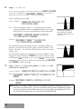
2
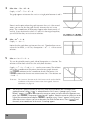
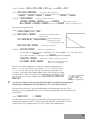
Graph y 16x 2 11 so that a complete graph is shown.
First graph on a standard viewing window.
Casio fx-7700GE:
TI-81:
g m 16 ?
› + 11 e
Y m 16 | › + 11 G
TI-82/83:
Y m 16 [ › + 11 G
The standard viewing window does not show a complete graph. Try the
range [3, 3] by [5, 15] with a scale factor of 1 for both axes. When you
finish changing the range values, you do not need to reenter the equation.
Press 6 to exit the range menu and then press e to graph on a
Casio calculator. Just press G on a TI calculator.
This range shows the complete graph of the function, including its
intercepts, maximum point, and end behavior.
3
Graph y x4 3x3 7x2 x 2 so that a complete graph is shown.
Try the standard viewing window.
Casio fx-7700GE:
TI-81:
g?^4-3?
^3-7?›-?+2e
Y|^4-3|^3-7
|›-|+2G
TI-82/83:
Y[^4-3[^3-7
[›-[+2G
TI
The range [4, 6] by [70, 10] with scale factors of 1 for the x-axis and
10 for the y-axis shows a complete graph.
15
Trace and Zoom
●
Casio fx-7700GE
●
TI-81
●
TI-82/83
You can use a graphing calculator to find approximations of the coordinates of
points on the graphs of functions. These coordinates can be found with great
accuracy by using the trace and zoom features.
TRACE
1
The trace feature moves the cursor along the graph of a function and
displays approximations of the coordinates of points on the graph.
Graph y x 3 6 in the standard viewing window. Then trace to find the
coordinates of the x- and y-intercepts.
Casio fx-7700GE:
TI-81:
g?^3+6e
Y|^3+6G
TI-82/83:
Y[^3+6G
Now use the trace feature to determine the coordinates of the x- and
y-intercepts. On the Casio calculator, press S t and on a TI,
press T. Then use the left and right arrow keys to move along the
function to the intercepts. The coordinates of the point at the cursor are
displayed at the bottom of the screen. The approximate coordinates of the
intercepts are (1.8, 0) and (0, 6).
Sometimes you will need to approximate the coordinates of a point with greater
accuracy than is possible with tracing from a viewing window that shows a
complete graph. In these cases, the zoom feature is very helpful.
Zoom
The zoom feature allows you to adjust the viewing window to show
larger or smaller pieces of the graph of a function. Your calculator may
offer you many methods for zooming in or out on a graph.
Using the One way that you can zoom in or out on a graph is to manually
Range to change the range for the viewing window. For example, if you
Zoom
initially view the graph of y x3 3x2 7 in the standard viewing
window, you can see that the zero is between 2 and 1. Setting the
viewing window to [2, 1] by [1, 1] with scale factors of 0.1 on
both axes will allow you to make a closer approximation. You can
then repeat this process as often as you like until you reach the
desired accuracy or until you reach the limits of the calculator.
16
Box Zoom
Another method of zooming in that is available on the Casio
fx-7700GE and the TI calculators is box zoom. With box zoom, the
calculator prompts you to use the arrow keys to position the cursor
at two opposite corners of a box to make a new viewing window.
When you press the e or é key, the calculator redraws
the graph of the function in the range that you specified with the
box. Use the following steps to use box zoom to zoom in on a part
of the graph of a function displayed on the graphics window.
1. Press S Z on a Casio fx-7700GE or Ω on a
TI calculator. Select Box by pressing ¡ or 1.
2. The graphics screen will appear with a cursor blinking in the
center. Use the arrow keys to move the cursor to one corner of
the box you want to define. Press e on the Casio fx-7700GE
or é on a TI calculator.
3. Move the cursor to the opposite corner of the box you want to
define. Notice that as you move the cursor, the sides of the box
change. Press e or é and the calculator will redraw
the graph in the new viewing window.
The location, size, and shape of the zoom box will usually change
the appearance of a graph in a significant way. The x-coordinates
for points on the vertical sides of a zoom box and the y-coordinates
of the horizontal sides will automatically be made new Xmin, Xmax
and Ymin, Ymax settings for the viewing window once you zoom to
that box.
Note:
If you change your mind about zooming into a box before you
actually zoom into it, press S on the Casio calculator. If
you are using a TI calculator, press any menu key to access a
menu, G to return to the graphics screen, or ‹ ± to
return to the home screen.
If you attempt to locate the second corner of your box horizontally
or vertically with the first corner, no box is formed for the next
viewing window. In this case, the Casio fx-7700GE will not redraw
the graph. It will wait for you to move the cursor to form a box and
press e for the graph to be redrawn. If you locate the second
corner of a box horizontally or vertically aligned with the first on a
TI calculator, you will receive an error message. You will have to
quit and then reaccess the box feature through the zoom menu to
complete the zoom in process.
17
Zoom In and
Zoom Out
by Factors
A third method of zooming in and out, which uses factors, is available on
each graphing calculator. With zooming by factors, the calculator will enlarge
or reduce the graph around a chosen center point by a factor or factors that you
choose. On the Casio fx-7700GE and the TI calculators, you can choose
different factors for the two axes. For example, if you start with a standard
viewing window and choose 1.5 for the x-factor and 2 for the y-factor and
zoom in at the origin, the space occupied by 1.5 units on the x-axis or 2 units
on the y-axis will be occupied by 1 unit on the new graph. Thus, the range for
the new graph will be [6.67, 6.67] by [5, 5]. Use the following steps to use
factors to zoom in or out on a graph that is displayed on the graphics screen.
Casio fx-7700GE
and TI:
You may choose different factors for the x- and
y-axes when you zoom in or out on the Casio fx-7700GE and
the TI calculators. Use the following steps to choose the
factors and zoom in or out.
1. Choose the factors by pressing S Ω ™ on
a Casio fx-7700GE or Ω 4 on a TI. Enter the factors
and press e or é. On the TI-82/83, press
Ω ¶ 4 to access the screen for setting the zoom
factors.
2. To zoom in or out on a Casio fx-7700GE, if you wish to
zoom in around a point other than the center of the
screen, use the trace function to move the cursor to the
point. Then press S Z £ or S
Z ¢.
To zoom in or out on a TI, press Ω 2 or Ω 3.
The graphics screen will appear with a blinking cursor at the
center. Use the arrow keys to move the cursor to the point
that you want to be the center of the zoom and press
é. You do not need to press Ω again to zoom
in or out by the same factor. Use the arrow keys to move the
cursor to the new center and press é.
Note:
The standard viewing window on the Casio fx-7700GE is a
“friendly” window. If you graph a function on that window and
then trace along the graph, the x-coordinates change by 0.1 with
each tap of the ¶ and ª keys.
This is not the case on the TI calculators. When you use the
standard viewing window, the x-coordinates are “messy”
decimals. You can obtain a friendly window by using a
[4.7, 4.8] by [3.1, 3.2] setting on the TI-81. On the TI-82/83,
use [4.7, 4.7] by [3.1, 3.1].
18
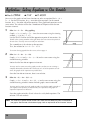
Systems of Equations
●
Casio fx-7700GE
●
TI-81
●
TI-82/83
You can use a graphing calculator to graph and solve systems of equations since
several equations can be graphed on the screen at one time. Graph the related
functions for the system. Then use the trace and zoom features to approximate
the solutions.
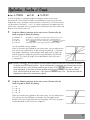
1
Graph the system of equations y 3.4x 2.1 and y 5.1x 8.3 in
the standard viewing window. Then determine the coordinates of the
intersection point(s).
Make sure your calculator is in the correct mode. If you are using a TI calculator,
clear all of the equations from the Y list first. If you are using a TI-82, you
may have to turn off statistical plots by pressing ‹ w 4 é.
Using the colon on the Casio calculators allows you to draw more than
one graph at one time.
Casio fx-7700GE:
TI-81:
g 3.4 ? + 2.1 ⁄ :
g m 5.1? + 8.3 e
Y 3.4 | + 2.1 é m 5.1 | + 8.3 G
TI-82/83:
Y 3.4 [ + 2.1 é m 5.1
[ + 8.3 G
Now use the trace function to determine the coordinates of the intersection
point. On the Casio calculators, press S t and on the TI
calculators, press T. Then use the left and right arrow keys to move
along the graph to the intersection point. The Casio fx-7700GE and the TI
calculators allow you to move from one function to another by pressing the
up and down arrow keys.
Use the box zoom or zoom in by factors to pinpoint the intersection
point. Repeatedly zooming and tracing allows you to find accurate
approximations for the coordinates of the point of intersection. The
coordinates of the point of intersection of y 3.4x 2.1 and
y 5.1x 8.3 are (0.73, 4.58) rounded to the nearest hundredth.
Note: The TI-82 and TI-83 have a special function on the CALC menu that will identify the point
of intersection of two graphs. When “5: intersect” is selected from the CALC menu, a
prompt saying “First curve?” appears. Move the cursor using § or • to select the first
function. Then use ¶ or ª to move the cursor close to the point of intersection. When
you are as close as you can get, press é. Use the same procedure to answer the
“Second curve?” prompt, except this time, press é twice. The cursor automatically
moves to the intersection, and the coordinates of that point are displayed at the bottom of
the screen.
19
2
Graph the system of equations y –x3 3x 2 9x and y –x2 10x 25.
Determine the coordinates of the intersection point(s).
Try graphing in the standard viewing window.
Casio fx-7700GE:
TI-81:
gm?^33? › + 9?
⁄:gm?
› + 10 ? - 25 e
Ym|^3-3|›+9|
é m | › + 10 | - 25 G
TI-82/83:
Ym[^3-3[›+9[
é m [ › + 10 [ - 25 G
The standard viewing window does not show a complete graph. You must
zoom out to view a complete graph so that you can determine how many
solutions exist. Zooming out to a window of [40, 40] by [40, 40] shows
that there is one solution to the system of equations. Now use the trace and
zoom in features to determine the approximate coordinates of the solution.
The coordinates of the intersection point are (2.30, 7.30) rounded to the
nearest hundredth.
3
2x 3
3
7
Graph the system of equations y x 1 and y 2 x 2 in the
standard viewing window. Determine the coordinates of the
intersection point(s).
Casio fx-7700GE:
TI-81:
g(2?T+3)/
(?-1)⁄
: g 1.5 ? - 3.5 e
Y(2|+3)/(|-1)
é 1.5 | - 3.5 G
TI-82/83:
Y(2[+3)/([-1)
é 1.5 [ - 3.5 G
The coordinates of the intersection points are (4.59, 3.39) and
(0.07, 3.39) rounded to the nearest hundredth.
Note: When a rational function has a vertical asymptote, your
calculator may or may not display the asymptote. Whether it
does or does not depends on the calculator you are using and on
the viewing window.
20
TI
Inequalities
●
Casio fx-7700GE
●
T1-81
●
T1-82/83
The Casio fx-7700GE and TI calculators allow you to graph inequalities on the
graphics screen. The procedures for graphing inequalities on a Casio fx-7700GE
are similar to the procedures for graphing functions. Graphing inequalities on a
TI requires using the “Shade(“ command from the draw menu and entering a
function for a lower boundary of the inequality and a function for the upper
boundary. The calculator graphs both functions and then shades above the first
function and below the second. Note that since this method draws on the
graphics screen instead of graphing through the Y list, editing these statements
requires the methods you use to evaluate expressions instead of those you use to
graph with the Y list.
When graphing a linear inequality on a TI calculator, you can use the Ymin range
value as the lower boundary if the inequality asks for “y ,” since the points that
satisfy the inequality are below the graph of the related equation. Use the Ymax
range value as the upper boundary if the inequality asks for “y ,” since the
points that satisfy the inequality are above the graph of the related equation.
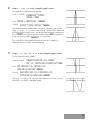
1
Graph y 3x 4 in the standard viewing window.
As with graphing functions, first clear the screen and set the range.
Casio fx-7700GE:
Place the calculator in inequality mode. Then press
g and choose the appropriate inequality symbol.
… 1 Ñ ¢ É Enter inequality (INEQ) mode.
Choose the symbol and enter
g¢3?
the inequality.
+4e
TI: The inequality asks for “less than or equal to,” so we will use Ymin as
the lower boundary and the expression for the related equation 3x 4
as the upper boundary. The boundaries are entered as an ordered pair
with the lower boundary first. Notice that by selecting “7” on the
DRAW menu the shade feature appears with the left parenthesis in
place. Be sure to enter the right parenthesis after the expressions.
TI-81:
‹Î7
Choose the shade option from the DRAW menu.
Vª4⁄,3|
+4)é
TI-82/83:
Enter the lower and upper boundary
expressions and close with a right
parenthesis. On the TI-82/83, it is not
necessary to use the ⁄ key before
,.
‹Î7V14,3[+4)é
Since both the x- and the y-intercepts of the line y 3x 4 are within the
standard viewing window, this is a complete graph of the inequality.
21
2
Graph y x 3 6x 2 8.
Be sure to clear the graphics screen before graphing. Press S 3 e
on the Casio fx-7700GE. Press ‹ Î 1 é on the TI since the
draw menu was used instead of the Y list to create the graph.
Try the standard viewing window.
Casio fx-7700GE:
g™?x3-6
?›+8e
TI-81: Since the inequality symbol is , the equation of the related
function should be entered as the upper boundary in the “Shade“
command. The Ymin value will be entered as the lower bound.
‹Î7Vª4⁄,|^
3-6|›+8)é
TI-82/83:
Note that the boundary is
not included in the graph
although it appears to be on
the screen.
‹Î7V14,[^
3-6[›+8)é
The standard viewing window does not show a complete graph of the
inequality, since the minimum of the graph is not on the screen. Try the
range [10, 10] by [30, 10] with a scale factor of 2 on the x-axis and
5 on the y-axis.
The command for graphing is the same on the Casio fx-7700GE, so after
changing the range values press 6 until you reach the text screen
and then press e to regraph. For a TI, press 6 and change the
appropriate values. Then return to the text screen by pressing ‹ ±.
Press é to redraw the graph.
3
Graph y > log (6x 3) in the viewing window [3, 5] by [3, 3] with
scale factors of 1 on both axes.
Casio fx-7700GE:
TI-81:
g¡i(6?+3)e
‹Î7K(6|+3)⁄,3)
é
TI-82/83:
‹Î7K(6[+3,3)
é
Note: For the TI calculators, using the DRAW menu to generate graphs of inequalities makes the
trace feature unavailable. Thus, you must use the free-moving cursor to explore these graphs.
You can use features from the zoom menu, but since only graphs generated from the Y list
are automatically redrawn you must re-execute the shade command.
22
Systems of Inequalities
●
Casio fx-7700GE
●
T1-81
●
T1-82/83
You can graph and solve a system of inequalities on a graphing calculator. When
graphing on a Casio fx-7700GE, you will use the colon to separate the
inequalities to be graphed. When graphing on a TI, you will use the shade
command with the two inequalities entered as the upper and lower boundaries
instead of a maximum or minimum value.
Since the TI graphs functions and shades above the first function entered and
below the second function entered, the first step in solving a system is to decide
which function to enter first as the lower boundary and which function to enter
second as the upper boundary.
A “greater than or equal to” symbol indicates that values on and above the graph
of the related function will satisfy the inequality. Similarly, a “less than or equal
to” symbol indicates that values on and below the graph of the related function
satisfy the inequality. Therefore, the related equation of the inequality with the
sign will be entered first, and the related equation of the inequality with the
sign will be entered second.
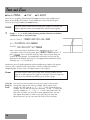
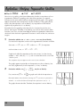
1
Graph the system of inequalities y 3x 5 and y 2x2 8 in the
standard viewing window.
Be sure to clear the graphics screen before graphing. Press S
3 e on the Casio fx-7700GE, or clear the Y list and press
‹ Î 1 é on the TI.
Casio fx-7700GE:
TI-81:
g¢3?-5⁄
:g£2?›-8e
‹Î72|›-8⁄,3|5)é
TI-82/83:
‹Î72[›-8,3[
-5)é
The points in the shaded area satisfy both y 3x 5 and y 2x 2 8.
2
4
Graph the system of inequalities y x2 and y > in the standard
x
viewing window.
Casio fx-7700GE:
TI-81:
g¢?›⁄
:g¡4/?e
‹Î74/|⁄,|›)é
TI-82/83:
‹Î74[,[›)é
23
The graphing calculator can be used to solve inequalities by shading the area on
the graph that makes the inequality true. To use this method, let each side of the
inequality represent a separate inequality and graph the system of inequalities.
3
Solve 5
x
3 3x 8 by graphing a system of inequalities.
x
3 y or y 5
x
3 and y 3x 8 as the
Use the inequalities 5
system of inequalities to be graphed.
Casio fx-7700GE:
TI-81:
g£R(5?-3)⁄
:g¢3?-8e
‹Î7‹R(5|-3)⁄,3
|-8)é
TI-82/83:
‹Î7‹R(5[-3),3
[-8)é
You can use the zoom feature to approximate a solution to the inequality.
You may use the trace and zoom features of the Casio fx-7700GE on
inequalities just as you do on functions. With a TI, the trace feature is not
available since we used the draw menu to create the graph. You must use
an arrow key to move the cursor to the edge of the shade and zoom in
using the zoom menu. Then press ‹ ± to return to the text screen
and press é to redraw the graph. The solution to the inequality is
x 4.05 to the nearest hundredth.
4
Solve 7x4 0.12x8 by graphing a system of inequalities on the viewing
window [10, 1] by [1, 3], with scale factor of 1 on each axis.
Casio fx-7700GE:
TI-81:
g£7^( ?+4)⁄
: g ¢ .1 ^ ( 2 ? +
8)e
‹ Î 7 7 ^ ( | + 4 ) ⁄ , .1
^(2|+8))é
TI-82/83:
‹ Î 7 7 ^ ( [ + 4 ) , .1 ^ ( 2
[+8))é
Zooming in shows that this inequality is true for x [–]4.00 to the nearest
hundredth.
Note: To graph a system of inequalities such as y > 2x 1 and y > x on the Casio fx-7700GE, use
the procedure described in Example 1 on the preceding page. Since the TI calculators require
one function to be the “bottom” function and the other to be the “top” function, you cannot
graph the system y > 2x 1 and y > x on a TI calculator by using the procedure
described here.
24
Rational Functions
●
Casio fx-7700GE
●
TI-81
●
TI-82/83
A rational function is one in which one polynomial is divided by another,
p(x)
q(x)
or in mathematical terms, f(x) where q(x) 0. Rational functions usually
have features that polynomial functions do not have, and the graphing calculator
is a good tool to explore these graphs.
Some graphs of rational functions are discontinuous. The breaks in continuity can
appear as asymptotes or as point discontinuities. A point discontinuity may not
be visible in the first viewing window that you use to graph a rational function, so
you may have to zoom in to see it or change the viewing window.
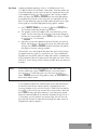
1
x 1
Graph y . Use a viewing window with scale factors of 1 for both axes.
x1
2
Since not all viewing windows allow you to see the point(s) of discontinuity, use
the appropriate window for your calculator.
Casio window: [ 4.7, 4.7] by [ 3.1, 3.1]
TI-81 window: [ 4,7. 4.8] by [ 5, 5]
TI-82/83 window: [ 4.7, 4.7] by [ 3.2, 3.2]
Casio fx-7700GE:
TI-81:
g(?›-1)/
(?+1)e
Y(|›-1)/(|+1)G
TI-82/83:
Y([›-1)/([+1
)G
TI
The graph looks like a line with a break in continuity at x 1.
Rational functions can also have asymptotes at values of x or y for which
discontinuities occur. An asymptote can either be vertical or horizontal.
Vertical asymptotes occur when the denominator equals zero. Horizontal
asymptotes can be found by solving the equation for x and considering
what number the function values are approaching as the absolute value of
x becomes very large. Both asymptotes can be found graphically by using
the zoom and trace features.
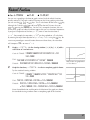
2
2x 3
Graph y x 1 . Use the viewing window [7, 7] by [5, 10] with
scale factors of 1 on both axes. Then find the equations of the vertical and
horizontal asymptotes.
Casio fx-7700GE:
g(2?+3)/(?
-1)e
25
TI-81:
Y(2|+3)/(|-1)G
TI-82/83:
Y(2[+3)/([-1)
G
First find the vertical asymptote by tracing along the graph and observing
the x-values near the discontinuity. As y increases, x approaches 1. On the
TI calculators, use the integer function on the Zoom menu to adjust your
viewing window. Press Ω 8. Then use the arrow keys to move the
cursor to the origin and press é. You can trace to a point where
x 1 and the calculator gives no y-value. This shows that the equation of
the vertical asymptote is x 1.
The horizontal asymptotes can be found by looking at the end behavior of
the function. You can trace along the function to find that as x increases, y
approaches 2. This can also be seen by graphing the function in a viewing
window with large absolute values of x, such as [1000, 1000] by
[5, 10], and tracing the function. The equation of the horizontal
asymptote is y 2.
In rational functions where the greatest exponent of the numerator is one
greater than the greatest exponent of the denominator, the graph exhibits a
2
x
slant asymptote. For example, f(x) has the line y x 6 as a
x6
slant asymptote and the line x 6 as a vertical asymptote.
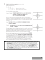
3
x 3x 4
Graph y in the standard viewing window. Determine the
x
2
equation of the slant asymptote and graph it on the screen.
Casio fx-7700GE:
TI-81:
g(?›+3?-4)
/?e
Y(|›+3|-4)/|G
TI-82/83:
Y([›+3[-4)/
[G
The slant asymptote is found by writing the expression as a quotient.
4
x 2 3x 4
x 3 x
x
4
As x approaches positive or negative infinity, approaches 0, which
x
4
means that x 3 approaches x 3. Therefore, the equation of the
x
asymptote is y x 3. Use the keystrokes below to graph this equation.
Use Y2 on a TI calculator.
Casio fx-7700GE:
TI-81:
Y|+3G
TI-82/83:
26
g?+3e
Y[+3G
The asymptote may not
appear in all viewing
windows.
Radical Functions
●
Casio fx-7700GE
●
●
TI-81
TI-82/83
You can use a graphing calculator to graph various kinds of radical functions
quickly and easily. To graph a radical function on the Casio graphing calculator,
you can use the R, ã, or ß keys. The TI calculators do not have a ß key,
although the TI-82/83 calculators do have ß on the MATH menu that you
access by pressing the µ key. On the TI-81, except for functions that use
R or ã, graphs of radical functions require that you use fractional exponents.
If you have an equation of the form y x, enter it into the calculator as
n
1
3 can be graphed on a TI calculator
y x n . For example, the equation y x
4
3
by entering the equivalent equation of y x 4 or y x 0.75 using the ^ key. Be
sure to use parentheses around fractions because without them, the calculator
3
will interpret x ^ 4_ to mean x3 4.
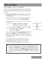
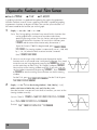
1
Graph y x
3 1 in the viewing window [1, 6] by [1, 6] with a
scale factor of 1 on both axes.
Casio fx-7700GE:
TI-81:
Y‹R(|-3)+1G
TI-82/83:
2
gSR(?-3)
+1e
Y‹R([-3)+1G
Why is there no graph when
x is less than 3?
Graph the function y 3
x
4 4 so that a complete graph is shown.
5
Try the standard viewing window.
Casio fx-7700GE:
TI-81:
g5Sß(3?+4)
-4e
Y ( 3 | + 4 ) ^ 0.2 - 4 G
TI-82/83:
Y ( 3 [ + 4 ) ^ 0.2 - 4 G
or Y 5 µ 5 ( 3 [ + 4 ) - 4 G
Since the end behavior and the point of inflection of the graph are shown,
the standard viewing window shows a complete graph of the function.
27
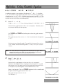
Quadratic Relations
●
Casio fx-7700GE
●
TI-81
●
TI-82/83
You can use a graphing calculator to graph relations; however you must do some
algebra before you graph. A graphing calculator will only graph functions, so
quadratic relations that are not functions must first be written as a combination of
functions. For example, the equation of the parabola x y 2 cannot be entered
directly into the graphing calculator. We must solve the equation for y. In this
case, you obtain y x. To graph, you must enter the two functions y x
and y x.
1
Graph the parabola whose equation is x y 2 5y 22 in the viewing
window [0, 30] by [10, 10] with scale factors of 1 on both axes.
First, solve the equation for y.
x y 2 5y 22
x 6.25 (y 2 5y 6.25) 22
Complete the square.
x 6.25 (y 2.5)2 22
Simplify.
x 15.75 (y 2.5)2
x
15
.7
5 y 2.5
x
15
.7
5 2.5 y
Subtract 22 from each side.
Take the square root of each side.
Subtract 2.5 from each side.
Now enter the two equations y x
15
.7
5 2.5 and
y –x
15
.7
5 2.5 into the graphing calculator. Since both of
these equations are functions, they can be graphed on a graphing
calculator.
Casio fx-7700GE:
TI-81:
g S R ( ? - 15.75 ) 2.5 ⁄ : g m S
R ( ? - 15.75 ) - 2.5 e
Y ‹ R ( | - 15.75 ) - 2.5 é m
‹ R ( | - 15.75 ) - 2.5 G
TI
TI-82/83:
28
Y ‹ R ( [ - 15.75 ) - 2.5 é
m ‹ R ( [ - 15.75 ) - 2.5 G
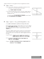
2
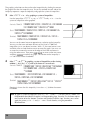
Graph the circle whose equation is x 2 y 2 16.
Solve the equation for y.
x 2 y 2 16
y 2 16 x 2
y 16
x2
Subtract x 2 from each side.
Take the square root of each side.
Use the standard viewing window.
Casio fx-7700GE:
g S R ( 16 - ? › )
⁄:gmSR
( 16 - ? › ) e
The Y-vars menu on the TI calculators allows you to use the name of a
function as a variable in other expressions. In this case, we will define one
of the two functions for graphing a circle as Y1 and then define the second
function as Y1.
TI-81:
Y ‹ R ( 16 - | › ) é m ‹
@1G
TI-82/83:
Y ‹ R ( 16 - [ › ) é ‹ m
@11G
The graph appears to be an ellipse even though it is actually a circle. Since
the viewing window is not scaled so that one unit on the x- and y-axes are
displayed as an equal length, the graph is distorted. Thus, the scales must
be adjusted so that the units on the x- and y-axes are equal in length.
TI
You can make the graph square on the TI calculators by pressing Ω
5. On the Casio fx-7700GE, press 6 ¡ 6 6 e.
The range produced on the Casio calculators is square, but in this case the
range does not allow you to see a complete graph. We must use a multiple
of this “default range” to view a complete square graph. Use [9.4, 9.4] by
[6.2, 6.2] with a scale factor of 1 for both axes. This viewing window
gives a complete graph of the functions and the graph appears as a circle.
Note: The TI-82 has a special circle function on the DRAW menu which will draw a circle, given
the coordinates of its center and its radius. To draw a circle from the home screen, press
‹ Î and select item 9:Circle(. The command “Circle(“ appears on the screen.
Enter the x-coordinate of the center followed by a comma, the y-coordinate followed by a
comma, and the radius followed by the closing parenthesis. Then press é. For
example, to draw a circle with center (2, 3) and radius 4, press ‹ Î 9 2 , 3
, 4 ) é. Displaying a circle via the DRAW menu does not permit you to trace
along the upper or lower half of the circle.
29
Trigonometric Functions and Their Inverses
●
Casio fx-7700GE
●
TI-81
●
TI-82/83
A graphing calculator is a good tool for exploring the graphs of trigonometric
functions and their inverses. Since a graphing calculator is capable of graphing
trigonometric functions in degrees or radians, be sure that your calculator is in
the correct mode for the function you wish to graph.
1
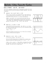
Graph y cos x for 360° x 360°.
Casio: The Casio graphing calculators have several built-in functions that
can be graphed with a minimum of keystrokes and without
specifying the range values. The sine, cosine, and tangent functions
are three of the built-in functions. To use a built-in function, press
g and the name of the function only, do not enter x.
To put the Casio fx-7700GE in degree mode, press S $
¡ e. The viewing window is automatically set to [360, 360]
by [1.6, 1.6] when the built-in cosine function is entered.
Press g c e.
TI: You must set the range values and then enter the equation for the
function much as you would write it with pencil and paper. First, check
to see that you are using degrees by pressing the 5 key. If not,
use the arrow keys to select “Deg” (or “Degree”) and press é.
You can then set the viewing window manually. If you wish, you can
set the window automatically by pressing Ω 7. Press fi
or W to see what settings your calculator uses for the viewing
window.
For the TI-81, press Y C | G. For the TI-82/83, press
Y C [ G.
2
1
Graph y 2 sin x. Use the viewing window [540, 540] by [3, 3]
2
with a scale factor of 90 for the x-axis and 1 for the y-axis.
Since the function is not one of Casio’s built-in functions, you must set the
viewing window manually.
Casio fx-7700GE:
TI-81:
Y2b(|/2)G
TI-82/83:
30
g2v(?u/2)e
Y2b([/2)G
Graphing calculators can also graph the inverses of trigonometric functions.
3
Graph y Arccos x.
Casio: Arcsin, Arccos, and Arctan are also built-in functions on Casio
calculators, so you do not need to set the range.
Press g S c e.
TI: The range will need to be set on the TI calculator. A good window to
use is [1, 1] by [20, 180] with a scale factor of 0.5 on the x-axis
and 90 on the y-axis.
For the TI-81, press Y ‹ C | G. For the TI-82/83,
press Y ‹ C [ G.
4
x
Graph y sin Sin–1 x Cos–1 in the viewing window [–, ] by
2
1
[2, 2] with a scale factor of on the x-axis and on the y-axis.
3
2
Begin by putting your calculator in radian mode. On the Casio fx-7700GE,
press S $ ™ e. On the TI calculators, access the mode
menu and highlight “Rad” or “Radian” using the arrow keys and the
é key.
The Casio fx-7700GE and the TI-82/83 will allow you to enter operation
symbols and constants like directly into the range. If you are using a
TI-81 calculator, you must manually enter a decimal approximation into
the range.
Casio fx-7700GE:
TI-81:
gv(Sn?S9(?/2))e
Yb(‹"|-‹#(
|/2))G
TI-82/83:
Yb(‹"[-‹#(
[/2))G
31
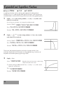
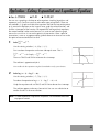
Exponential and Logarithmic Functions
●
●
Casio fx-7700GE
TI-81
●
TI-82/83
A graphing calculator can be used to graph exponential and logarithmic
functions just as it is used to graph other types of functions. Even functions that
would be tedious and time consuming to draw by hand can be graphed quickly.
1
Graph y 92x in the viewing window [7, 1] by [1, 9] with a scale
factor of 1 on each axis.
Be sure that your calculator is in rectangular coordinate mode.
Casio fx-7700GE:
TI-81:
Y9^(2+|)G
TI-82/83:
2
g9^(2+?)e
Y9^(2+[)G
1 32x
Graph y – 2
. Use the viewing window [–5, 5] by [–10, 2] with a
scale factor of 2 on each axis.
Casio fx-7700GE:
TI-81:
g m 0.5 ^ ( 3 - 2 ? ) e
Y m 0.5 ^ ( 3 - 2 | ) G
TI-82/83:
Y m 0.5 ^ ( 3 - 2 [ ) G
The natural and common logarithms are built-in functions on the Casio
calculator. Recall that built-in functions can be graphed using a minimum of
keystrokes and without specifying the range values.
3
Graph y ln x.
Casio:
ghe
Remember that you do not enter x when using
a built-in function on the Casio.
TI: Set the viewing window on the TI to [1, 8] by [1, 3] with a scale
factor of 1 on each axis.
TI-81:
YJ|G
TI-82/83:
32
YJ[G
Graphing calculators can be used to graph logarithmic functions with base 10 or
base e. If you wish to graph a logarithmic function with another base,
log x
log a
ln x
ln a
you must use the change of base formula, loga x or loga x .
4
Graph y log4 x. Use the viewing window [1, 5] by [3, 3] with a scale
factor of 1 on each axis.
log x
log 4
Using the change of base formula, log4 x .
Casio fx-7700GE:
TI-81:
gi?/i4e
YK|/K4G
TI-82/83:
YK[/K4G
The graph of the equation has a vertical asymptote at x 0. It may appear
that the graph starts at x 0, but actually the calculator cannot graph
enough values to show the true behavior of the graph. As always, it is
important to know how to interpret the graph that the calculator draws.
The domain is x > 0, and the range is the set of real numbers.
5
Graph y log6 (3 x) in the viewing window [8, 4] by [5, 5] with a
scale factor of 1 on each axis.
Casio fx-7700GE:
TI-81:
gmi(3-?)/
i6e
Y-K(3-|)/K6G
TI-82/83:
Y m K ( 3 -[ ) / K 6 G
33
Application: Solving Equations in One Variable
●
Casio fx-7700GE
●
TI-81
●
TI-82/83
You can use the graphs of two linear functions to solve an equation like 3x 6 5x 2. For the first function, let y one side of the equation. For the second
function, let y the other side of the equation. Then graph both equations on the
same screen. The solution will be the x-coordinate of the point where the two
functions intersect.
1
Solve 3x 6 5x 2 by graphing.
Graph y 3x 6 and y 5x 2 on the same screen using the viewing
window [3, 16] by [5, 25].
Use the TRACE function to find the approximate point of intersection. The
TRACE in the viewing window at the right shows the exact intersection point of
the two lines. This may not occur with your calculator.
The x-coordinate is the solution to the equation.
Thus, the solution for 3x 6 5x 2 is 4.
To review clearing graphs from the screen, refer to page 9.
2
Solve 3x 6 4x (x 10).
Graph y 3x 6 and y 4x (x 10) on the same screen using the
standard viewing window.
Notice that the lines do not appear to intersect.
You may wish to zoom out on the graph to make sure that you are viewing a
complete Remember that when the coefficients of x in linear equations are the
same, the graphs of the equations are parallel lines.
Since the lines do not intersect, there is no solution.
3
Solve 4(x 2) 6x 2(4 x).
Graph y 4(x 2) and y 6x 2(4 x) on the same screen using the
standard viewing window. Notice that both graphs seem to coincide.
You may wish to zoom in on the graph to make sure that the graphs coincide. If
you simplify each equation you will find they are equivalent. The graphs of
equivalent equations are identical.
Since the graphs coincide, all real values of x satisfy both equations. The
solution is all real numbers.
Note: The TI-82 has a special function on the CALC menu that will identify the point of intersection of
two graphs. See the note at the bottom of page 19 for an explanation of the “intersect” feature.
34
Application: Solving Quadratic Equations
●
Casio fx-7700GE
●
TI-81
●
TI-82/83
A quadratic equation is an equation in the form of Ax2 Bx C 0, where
A 0. The solutions for this type of equation can be estimated by graphing the
related function, y Ax2 Bx C and locating those points where y 0. The
x-coordinates of these points are called the zeros of the function. The zeros of a
function are the roots to the associated equation.
1
Solve 2x2 x 15 0.
Graph y 2x2 x 15. Use a viewing window of [10, 10] by [16, 4].
Notice that the graph intersects the x-axis in two places. Therefore, there
are two real solutions for the equation.
Use Ω and T to find the points where the graph intersects
the x-axis.
The graph intersects the x-axis at (2.5, 0). One solution for the equation
is 2.5.
Continue to trace along the graph. The graph also intersects the x-axis at
(3, 0). Another solution for the equation is 3. Always check your estimated
solution.
Note: The TRACE function can only give you the coordinates of the graph dot that
appears to lie on the x-axis. Often you may not be able to find the exact
x-coordinate for the point where the y-coordinate is zero.
2
Solve x2 10x 25 0.
Graph y x2 10x 25.
Notice that the graph appears to intersect the x-axis at one point.
Whenever there appears to be a single point of intersection, it is a good
idea to zoom in on that point, because the graph could intersect the axis
in two points very close together, or not intersect the axis at all.
Zoom in on the point. Then use T to determine the x-coordinate of
the point where the graph intersects the x-axis.
The graph intersects the axis at (5, 0).
The solution is 5.
35
3
Solve 10x2 51x 65 0.
Graph y 10x2 51x 65 0.
The graph appears to intersect the x-axis at a single point between 2 and 3.
Zoom in on the point where the graph intersects the x-axis. After several
zooms, you can see that the graph actually intersects the axis in two
points. The x-coordinates of these points appear to be almost exactly 2.5
and 2.6. If you substitute the values 2.5 and 2.6 in the original equation,
you will find that they are in fact exact solutions.
4
Solve 8x2 1 0.
Graph y 8x2 1.
Notice that the graph does not intersect the x-axis. Therefore there are no
values of x for which y 0. Thus, the equation 8x2 1 0 has no real
solutions.
5
Solve x2 3x 5 2 x.
This can be solved by treating each side of the equation as a function. The
solutions will be those values of x that satisfy both functions.
Graph y x2 3x 5 and y 2 x on the same screen. The solutions
will be the x-coordinates of the points where the tow graphs intersect.
Use T to determine the x-coordinate of each intersection. Use
Ω to determine the most accurate estimates for x. The solutions are
3 and 1.
TI-82 note: The “intersect” function on the CALC menu can be used to find the
coordinates of the points of intersection of two graphs. For more
information, see page 19.
Note:
36
The TI-82 has a special function on the CALC menu that will identify the x-intercept of the
graphed function. When “2:root” is selected from the CALC menu, a prompt saying “Lower
bound?” appears. Use ¶ or ª to move the cursor to a point just to the left of the apparent zero
point. Press é. The prompt “Upper bound?” appears. Move the cursor to a point just to the
right of the estimated zero and press é. A prompt saying “Guess?” appears, asking you to
move the cursor as close as you can to the point you think the zero occurs. Press é and
the nearly exact coordinates of the actual x-intercept appear.
Application: Families of Graphs
●
Casio fx-7700GE
●
TI-81
●
TI-82/83
A family of graphs is a group of graphs that displays one or more similar
characteristics. Many linear functions are related because they have the same
slope or the same y-intercept as other functions in the family. All linear functions
can be written in the form y mx b, where m represents the slope of the line
and b is the y-intercept. You can graph several functions on the same screen and
observe if any family traits exist.
1
Graph the following functions on the same screen. Then describe the
family of graphs to which they belong.
y 0.5x 1
yx1
y 3x 1
y 5x 1
Remember, to graph several functions on the same screen
on the Casio calculator you must use a multistatement.
Press g, enter the equation, press ⁄ :, then
repeat the steps, connecting equations with the colon.
Use the standard viewing window.
When all functions are graphed on the same screen, you can observe that
they are all lines and that they all pass through the point (0, 1). However,
their slopes are different. If you compare each graph with its slope, you
find the greater the slope, the greater the angle formed by the line and
the x-axis. This family of graphs can be described as lines that have a
y-intercept of 1.
Note: On the TI calculators, you can suppress any of the graphs to observe each one in comparison to another.
To do this, press Y. Notice that the sign in each equation is highlighted. Use the arrow keys to move
the cursor over the of the function you do not wish to graph. Press é. Notice the sign is no
longer highlighted. That function will not be graphed when you press G. To graph the function
again, use the arrow key to move to the sign and press é again. The sign will once again be
highlighted and the function will again be graphed.
2
Graph the following functions on the same screen. Then describe the
family of graphs to which they belong.
y 3x
y 3x 1
y 3x 2
y 3x 5
When all functions are graphed on the same screen, you can observe that
they are lines that have different y-intercepts, but they appear to be
parallel. Lines that are parallel have the same slope. This family of graphs
can be described as lines that have a slope of 3.
37
Note: On the TI-82/83, families of functions are easily graphed using the bracket
keys, { and }, which are second functions of the parentheses keys. The
brackets are used to group those numbers that change when all of the other
parts of the equations are identical.
In Example 1, use the brackets to group the differing coefficients of x. Press
Y ‹ { .5 , 1 , 3 , 5 , } [ + 1. Then press
G and all of the functions will be graphed.
In Example 2, use the brackets to group the differing values of b. Press
Y 3 [ + { 0 , 1 , m 2 , 5 } G.
Quadratic functions whose graphs are parabolas can be written in the form
y k a(x h)2, where (h, k) represents the coordinates of the vertex of the
parabola. As with lines, there are families of parabolas that share common
characteristics. One family of parabolas may possess the identical shape, but
have different vertices. Another family may have the same vertex, but the shapes
of the parabolas differ.
3
Graph the following functions on the same screen. Then describe the
family of graphs to which they belong.
y x2
y (x 2)2
y (x 4)2 3
y x2 6
When all the functions are graphed on the same screen, you can observe
that the parabolas do not have the same vertex. However, all of the
parabolas open upward and have the same shape. The shape can be
described by the simplest function, y x2. This family of graphs can be
described as parabolas with the shape of the graph of y x2, translated to
different locations on the coordinate plane.
4
Graph the following functions on the same screen. Then describe the
family of graphs to which they belong.
y 0.5x2
y x2
y 4x2
y 8x2
When all the functions are graphed on the same screen, you can observe
that all of the parabolas have the same vertex and open downward.
However, the shapes of the parabolas differ with the coefficient of x2.
Notice that the greater the coefficient the narrower the opening. This is the
family of parabolas that open downward and have a vertex at the origin.
38
Application: Maxima, Minima, and Zeros of Functions
●
Casio fx-7700GE
●
TI-81
●
TI-82/83
You can use the graphing calculator to estimate the zeros and the relative
maximum and minimum points of a polynomial function. First you must graph
the function. Then use TRACE and ZOOM to determine the coordinates of the
point(s) you desire.
1
Approximate the maximum, minimum, and zeros of y x 2 3x 4.
First graph the function.
The graph is a parabola opening downward that intersects the x-axis at
two points. Therefore, the function has a maximum, no minimum, and
two zeros.
Use the TRACE function to locate the approximate coordinates of the
maximum. Use the arrow keys to find the point where the y-coordinate
displayed at the bottom of the screen appears to be greatest.
Remember that the coordinates that appear at the bottom of your calculator‘s
screen may not match those shown at the right.
Once you have located the approximate maximum, use the ZOOM feature
to enlarge your graph. Then use the TRACE function again to gain more
precise coordinates. The maximum occurs at approximately ( 1.50, 6.25).
If you use the Box Zoom feature to create a rectangle similar in shape to that of the
viewing window, the curve will maintain its parabolic shape while zooming in on
the desired area.
The coordinates of the zeros can be found in a similar way by using TRACE
to find the point(s) where the graph crosses the x-axis and then using
ZOOM to fine-tune your coordinate readings. The two zeros of this
function are at approximately 4.00 and 1.00. If you substitute these
values for x in the quadratic expression, you will find that they are, in fact,
the exact zeros of the function.
TRACE Note: Because graphing calculators differ, your readings may not match
those given here. Remember that the TRACE function gives you
the coordinates of the dots on the grid and not every value
along the curve.
39
2
Approximate the maximum, minimum, and zeros of y 2x3 x2 5x 3
to the nearest hundredth.
First graph the function.
The graph appears to have a relative maximum, a relative minimum, and
three zeros. Use TRACE and ZOOM to refine your estimates of the
coordinates of each point.
The relative maximum occurs at about (1.09, 1.05). The relative
minimum occurs at about (0.76, 5.34). The three zeros occur at about
1.50, 0.62, and 1.62.
3
Approximate the maxima, minima, and zeros of y x4 5x2 6.
Graph the function. The graph appears to have two relative minima, one
relative maximum, and two zeros.
However, if you zoom in on the function, you will find that there are
actually four zeros. These zeros are about 1.73, 1.41, 1.41, and 1.73.
By zooming in on other parts of the curve, you will find the relative
minima occur at about ( 1.58, 0.25) and (1.58, 0.25). The relative
maximum occurs at (0, 6).
Note: The TI-82 and TI-83 have special functions that will find a zero, a minimum, or a maximum of the
function you have graphed. These special functions can be accessed on the CALC menu, which
is the second function of the T key. The second item 2:root finds the zero of a function.
The third and fourth selections find the minimum and maximum, respectively. For each of these
functions, you are asked to define the interval in which you wish the calculator to search for a
particular point. The following directions apply to each function.
• Graph the function. Access the CALC menu.
• Select the point you wish to find (2:root, 3:minimum, or 4:maximum)
• Your graph will be displayed with a prompt at the bottom saying “Lower Bound?” Move the
cursor to the point you wish to be the lower bound for the interval in which you wish to find a
particular point. Press é.
• A second prompt saying “Upper Bound?” will appear. Once again, move the cursor to the point
which represents the upper bound of the interval in which you wish to find a particular point.
Press é.
• A third prompt saying “Guess?” appears. Move the cursor to the point at which you think the
point occurs and press é. The cursor will then move to the exact point and the x- and ycoordinates will appear at the bottom of the screen.
40
Application: Solving Trigonometric Equations
●
Casio fx-7700GE
●
TI-81
●
TI-82/83
You can use a graphing calculator to solve a trigonometric equation in the same
way you have used it to solve linear equations, quadratic equations, and systems
of equations.
1
Solve tan x sin x • cos x if 360° x 360°.
Make sure your calculator is set for degree measure. Set the RANGE for
x-values greater than the given interval, say [450°, 450°] with a scale
factor of 90°. For the y-axis, use [3, 3] with a scale factor of 1.
Graph y tan x and y sin x • cos x on the same screen. Then use
TRACE and ZOOM to locate the points of intersection in the interval
360° to 360°. The x-coordinates of those points are the solutions to the
equation. The solutions are 360°, 180°, 0°, 180°, and 360°.
2
Solve 2 cos x 4 0 if 0° x 360°.
Set the RANGE for the viewing window [90°, 450°] by [8, 2]. Since
one side of the equation equals zero, you will use the method for finding
the x-intercepts of a function.
Graph y 2 cos x 4.
Notice the graph does not intersect the x-axis. There are no x-intercepts
and, thus, no solutions for the equation.
3
Solve sin 3x cos 2x 1 if 0° x 360°.
Use the viewing window [90°, 450°] by [5, 5].
You can also solve the equation by first algebraically manipulating the
equation to get 0 on the right-hand side: sin 3x cos 2x 1 0.
Graph y sin 3x cos 2x 1. Then find the x-intercepts of the function
by using TRACE and ZOOM. The solutions are 0°, 40.6°, 139.4°, 180°,
and 360°. The decimal values are approximations.
41
Application: Verifying Trigonometric Identities
●
●
Casio fx-7700GE
TI-81
●
TI-82/83
You can use a graphing calculator to determine whether an equation may be a
trigonometric identity by graphing each side of the equation as a separate
function on the same screen and then comparing the two graphs. If the graphs
appear to coincide, then the equation may be an identity. If the graphs do not
match, then the equation is not an identity. Any equation must be verified
algebraically to prove that it is an identity.
Remember that the graphing calculator only has function keys for the sine,
cosine, and tangent. Therefore, if the identity you wish to verify contains other
functions, you must use your knowledge of the basic trigonometric identities to
substitute values for these trigonometric functions in terms of the sine, cosine, or
tangent.
1
Determine whether tan x cot x sec x • csc x may be an identity.
First rewrite the equation in terms of the trigonometric functions available.
1
1
1
Since cot x , sec x , and csc x , the equation
tan x
cos x
sin x
1
1
1
can be written as tan x .
tan x
cos x sin x
Graph each side of the equation on the same screen. Use the viewing
window [360°, 360°] by [5, 5], with a scale of 90° for the x-axis and
1 for the y-axis.
The asymptotes may not appear on the screen of your calculator.
The graphs appear to coincide, so the equation may be an identity. You
can verify algebraically that the equation is, in fact, an identity.
2
TI-81
x
2 cos x
Determine whether cot may be an identity.
2
1 2 sin x
x
1
x
First, rewrite cot as tan . 2
2Then
graph each side of the equation on
x
the same screen. Note that when entering tan 2 , you must use parentheses
around x 2 or the calculator will interpret the expression as (tan x) 2.
The graphs do not coincide. Therefore, the equation is not an identity.
TI-81
42
Application: Solving Exponential and Logarithmic Equations
●
Casio fx-7700GE
●
●
TI-81
TI-82/83
You can use a graphing calculator to solve equations involving logarithms and
exponents just as you have used it to solve other types of equations. There are
two methods: (1) graph each side of the equation and find the intersection points
or (2) rewrite the equation so that it equals zero, graph the related function, and
find the x-intercepts of the function. For exponential and logarithmic equations,
the second method is often easier because it is easier to see where the graph
crosses the x-axis than it is to see the point(s) of intersection. Often a point of
intersection is near an asymptote and the gradual decrease or increase can make
that point of intersection difficult to find.
1
1
3x 6x2.
Solve 4
Use the viewing window [2, 4] by [3, 3].
First transform the equation so that one side equals zero. That is
1
1
4 3x 6x2 0. Graph y 4 3x 6x2.
Then use TRACE and ZOOM to locate the x-intercept.
The solution is approximately 0.6.
TI
You could solve the equation using the first method to verify your solution.
2
Solve log (x 3) log (7 4x).
Use the viewing window [5, 5] by [3, 3].
Transform the equation to log (x 3) log (7 4x) 0.
Graph the equation and use TRACE and ZOOM to locate the x-intercept.
The solution appears to be very close to 0.8. You can use substitution to
confirm that 0.8 is the exact solution.
TI-81
Note: To solve exponential or logarithmic inequalities, use the methods described
on pages 21 and 22.
43
Entering Matrices
●
Casio fx-7700GE
●
TI-81
●
TI-82/83
Graphing calculators make many of the tedious paper-and-pencil operations with matrices
quick and simple. Each calculator has different matrix capabilities, but they all work through
matrix menus. Suppose you wanted to enter the matrix 1 3 –6 .
2 –2 4
Casio fx-7700GE: The Casio fx-7700GE contains memories for five different matrices and a
special matrix answer memory. You can enter values into matrices A through
E. The answer matrix is used to store the result of a matrix operation. The
maximum dimensions for each matrix is 9 rows by 9 columns.
Before entering a matrix, you must be in matrix mode. Press … 5 and
then press ¢. The matrix list will be displayed.
To select matrix A, press ¡. The last elements of matrix A appear along
with a different menu at the bottom of the screen.
If this matrix A has the same dimensions as the one you wish
to enter, you can proceed by entering the elements of the
desired matrix. Press 1 e 3 e 6 e 2 e
2 e 4 e. As you press each number, it appears at the
bottom of the screen. When you press e, the number
appears in the matrix, and the highlight moves on to the next
element to be entered.
A
1
2
1
1
2
2
3
–2
3
–6
4
If matrix A does not have the same dimensions as the one you wish to enter,
you can change the dimensions by pressing ™ which designates the
dimensions of the matrix. Enter the appropriate number of rows and then press
e. Then enter the number of columns and press É. You will return to
the matrix list showing a 2 3 matrix. Follow the directions given above to
select matrix A and enter the correct numbers.
You can enter another matrix in the same way, but select matrix B instead of
matrix A on the first matrix menu.
TI-81:
The TI-81 contains memories for three matrices, A, B, and C. You can enter
values into all three matrices and use them in operations. Each matrix has a
maximum dimension of 6 6. There is no matrix mode on the TI calculators.
To enter a matrix, press N. A menu of matrix
operations appears. Use the arrow key to go to the EDIT
menu. A list of three matrices and their dimensions appears.
Select whichever matrix you wish by using the up and down
arrows to highlight your selection and press é.
44
MATRIX EDIT
1: [A]
66
2: [B]
32
3: [C]
33
If the matrix you chose has the same dimensions as the matrix
you wish to enter, press é twice. Element 1, 1 (row 1,
column 1) is highlighted. Enter the number you want and
press é. Continue the process until all values are
entered.
If the matrix you chose does not have the same dimensions as
the matrix you wish to enter, press the number for the number
of rows and é. Then press the number of columns and
é. Proceed as shown above to enter each element.
When you finish entering the values of your matrix, press
‹±. The home screen appears. To view the matrix,
press ‹ \, which is the second function of the 1 key.
Then press é. The matrix will appear on the screen.
[A] 2 3
1,1 1
1,2 3
1,3 –6
2,1 2
2,2 –2
2,3 4
[A]
[1 3 –6]
[2 –2 4 ]
Notice that the second functions of the 2 and 3 keys, access matrices
B and C, respectively.
You can enter the other two matrices in the same way, by
selecting the appropriate matrix on the EDIT menu.
TI-82:
The TI-82 has memories for five matrices, A, B, C, D, and E.
You can enter values into all five matrices. The maximum
dimensions for each matrix is 99 99.
Entering a matrix on a TI-82 calculator is similar to the process
described for the TI-81. To enter a matrix, press N and
use the arrows to highlight EDIT. The list of five matrices
appears. Use the up and down arrows to select whichever
matrix you wish to define and press é. You change the
dimensions of the matrix in the same way as the TI-81.
Once the matrix dimensions are defined, a matrix of those
dimensions appears on the screen. In a newly-defined matrix,
all the values are zeros. In a previously-defined matrix, the
values are those entered when the matrix was defined. The
first element (row 1, column 1) is highlighted. Enter the first
value and press é. Then use the arrow keys to move to
the new value you wish to enter. When you have completed
the entries, you can exit the screen by pressing ‹ ±.
MATRIX [A] 2 3
[1 3 –6]
[2 –2 4 ]
1,1 1
Note: If you enter a large matrix, not all of the columns and/or rows may appear on the screen. To
view other portions of the matrix, you can use the arrow keys to scroll to the portion of the
matrix you wish to view.
45
Determinants, Inverses, and Operations
●
Casio fx-7700GE
●
TI-81
●
TI-82/83
The graphing calculator has simplified the tasks of finding determinants and
inverses of matrices to the pressing of only a few keys.
1
Find the determinant of matrix A if A 1 3 .
2 –2
Enter the matrix into your calculator.
Casio fx-7700GE: Press É É ™ ¡ ⁄ A e.
The determinant appears.
Press ¡ ⁄ A ∞ to return to the original
matrix screen.
TI-81: Press N. Then select 5:det. Then name the matrix you want
by pressing ‹ \ and é to calculate the determinant.
TI-82/83: From the home screen, press N and use the arrow keys to
highlight the MATH menu. Use the arrow keys to highlight item
1:det and press é. To select the matrix, press N
and highlight the NAMES menu. Use the arrow key to highlight
the matrix you want and press é. Press é again to
perform the calculation.
The determinant of matrix A is 8.
2
Find the inverse of matrix A if A 1 3 .
2 –2
Casio fx-7700GE: Press ¡ ⁄ A S ¤ e.
`
[A]–1
[.25 .375]
[.25 –.125]
The inverse appears.
Press ¡ ⁄ A ∞ to return to the original
matrix screen.
TI-81: Press ‹ \ ¤ é.
TI-82/83: Press N and select the matrix you want as described
above in Example 1. Press ¤ and é to perform the
calculation.
The inverse of matrix A is 0.25 0.375 .
0.25 –0.125
46
TI-81
Other operations with matrices that can be done with a graphing calculator
include scalar multiplication, multiplying two matrices, squaring a matrix, adding
and subtracting two matrices, and finding the transpose of a matrix.
Casio fx-7700GE: Once you have entered matrices A and B, you can add the
two matrices, subtract the two matrices, and multiply the two
matrices.
AB
Press ¡ ⁄ A + ¡ ⁄ B
e. The sum appears.
AB
Press ¡ ⁄ A - ¡ ⁄ B
e. The difference appears.
AB
Press ¡ ⁄ A u ¡ ⁄ B
e. The product appears.
Every time you do a calculation, the result is automatically
stored in the matrix answer. If you wish to use the results for
another computation, press É ª j. You can then
assign the matrix to C, D, or E for further computations.
To perform scalar multiplication, first input the multiplier, then
select the matrix you want to multiply and press e. The
result appears automatically.
TI:
To perform operations with matrices, you enter them in an
expression in the same way you would enter a variable and
execute the calculation by pressing é. The only
difference in the operation of the two calculators is how the
matrices are called up into the expression.
To multiply matrices A and B on the TI-81, select matrix A by
pressing ‹ \. Then press u and select matrix B by
pressing ‹ ]. The expression [A] [B] appears in the
window. Press é to calculate the result.
To add matrices A and B on the TI-82, you must use the
NAME menu on the MATRX menu to name each matrix as it is
needed. The other operations are the same as with the
TI-81.
Note: On the TI-82/83, matrix expressions involving several operations are easy. Enter the
expressions in much the same form as you would write them. Evaluating a matrix expression
such as 3A 4B on the TI-81 or Casio fx-7700GE requires storing of intermediate results
and additional keystrokes. See the manual for your calculator for tips on evaluating such
expressions.
47
Statistical Computations
●
Casio fx-7700GE
●
●
TI-81
TI-82/83
In addition to graphing, graphing calculators are capable of doing intricate
computations, including finding statistical values for a set of data. The first step
on the Casio fx-7700GE is to choose the appropriate statistical mode for statistical
computations. This mode is called standard deviation mode. Press … 3. You
may choose to store the data for computations or to use the data once and
discard it. We will use the data storage mode. Enter data storage mode by
pressing S Ñ • • ¡. The keystrokes for non-storage mode
are S Ñ • • ™.
You must clear all of the statistical memories on your calculator before
performing any computations. If you forget to clear the memories, your
calculations may include old data values causing your results to be incorrect.
Casio fx-7700GE:
TI-81:
‹_ª2é
TI-82/83:
1
S0™
Clears the data in the memory.
Clears the data in the memory.
_4‹Lé_4‹lé
Clears data lists L1 and L2.
The prices for several bicycle helmets are given below. Find the mean, the
standard deviation, and the sum of the data. Then find the sum of the
squares of the data values and the standard deviation of a population for
which the data is a sample.
51
40
58
60
30
45
66
40
87
65
41
60
40
35
47
49
54
50
52
47
Enter the data into the calculator.
Casio fx-7700GE: 51 ¡ 40 ¡ 58 ¡ and so on 47 ¡
To correct a mistake in the data on a Casio fx-7700GE,
press ™ to access the data edit menu. Then locate
the incorrect data value with the arrow keys, type in the
correct data, and press e.
TI-81: Before you enter new data, clear any data that may have been
stored in the calculator. To do this, press ‹ _ ª 2
é. Data is always entered as a data pair. So, when you wish
to analyze a set of single data points, the y-value of the data pair
represents the frequency of the occurrence of the x-value. For
example, the data pairs (9, 1) and (11, 3) represent one occurrence
of the data value 9 and three occurrences of the data value 11.
When the data memory is cleared all y-values are set to 1, so
pressing é when the cursor is on the y-value will accept this
frequency.
48
‹_ªé
Accesses the data edit option.
51 ééé 40 éé 58
éé and so on 47 é é
TI-82/83: Data is entered individually into a list. Before you enter new
data, clear data that may have been previously stored in data list
L1. Press _ 4 ‹ L é. Use the following
procedure to enter the new data.
_é Accesses the data edit option.
51 é 40 é 58 é and so on 47 é
If you make a mistake entering data into your TI calculator, use
the arrow keys to move to the incorrect data and enter the
correct value. If you wish to delete an incorrect data point on a
TI-81, move the cursor to the “ ” for the x- or y-value of the
point and press D. Pressing I when the cursor is on the
“ ” allows you to insert a new data pair before that point. On
a TI-82, you can delete data by moving the cursor to the data to
be deleted and pressing D. To insert data at a desired point,
press ‹ I and enter the data.
Now that the data is entered, we can find the statistical values.
Casio fx-7700GE:
TI-81:
¢¡e
Chooses the mean from the standard deviation function menu
and calculates.
™e
Chooses the standard deviation from the standard deviation
function menu that is already displayed and calculates.
É∞™e
Exits to the previous menu, enters the data sum function
menu, then chooses and calculates the sum.
¡e
Chooses the sum of the squares from the data sum menu that
is already displayed.
É¢£e
Exits to the previous menu, enters the standard deviation
function menu, then chooses and calculates the standard
deviation of the population.
‹ _ éé
TI-82/83:
Chooses 1-VAR from the statistics calc menu.
_¶1é
_
Notice that the TI calculators display many statistics at one time. x denotes the
mean, x is the sum, x 2 is the sum of the squares, Sx is the standard deviation
of a population for which the data is a sample, x is the standard deviation of the
data given, and n is the number of data values. The TI-82 and TI-83 provide
additional statistical results.
To the nearest hundredth, the mean of the data is 50.85, the standard deviation is
12.59, the sum is 1017, the sum of the squares is 54,885, and the standard
deviation of a population for which the data is a sample is 12.92.
1-Var
x 50.85
x 1017
x2 54885
Sx 12.9178579
x 12.59077043
n 20
TI-81
49
2
Find the median of the test scores listed below on a TI calculator.
82
91
74
78
94
68
74
88
64
42
72
82
79
99
98
75
61
78
86
69
Only the Casio fx-7700GE and the TI-82/83 graphing calculators will
compute the median of a set of data for you. However, the TI-81 calculator
will sort data from least to greatest according to the x- or y-values so that
the median can be found easily.
Clear the data memory and enter the data into your calculator.
Casio fx-7700GE:
™£¡
Clear the data memory.
82 ¡ 91 ¡ 74 ¡ and so on 69 ¡
¢
Chooses the standard deviation function menu.
¢™e
TI-81:
‹_ª2é
Chooses the median from the
representative menu and calculates.
Clear the data memory.
‹ _ ª 82 é é
é and so on 69 é
TI-82/83:
_4‹Lé
_ é 82 é
and so on 69 é
Choose the data edit option
and enter the data.
Clear data list L1.
Choose the data edit option
and enter the data.
TI-81: Now sort the data using the xSort option under the statistics data menu.
‹_ª3é
We have 20 pieces of data, so the median is the average of the 10th
and 11th values. We can use the ≈ key, located above the 0 key,
to recall the x-value of a data point when we enter the number of
the data point in the set. This will allow us to find the mean of the
10th and 11th values.
( ‹ ≈ 10 ) + ‹ ≈ 11 ) ) / 2 é
TI-82/83: Find the single variable statistics.
_ ¶ éé
Use the down arrow key to scroll down to read the median
value which is listed as Med .
The median test score is 78.
50
Note: On the TI-81, the
y-values must all be 1 for
this technique to be
accurate.
Histograms
●
Casio fx-7700GE
●
TI-81
●
TI-82/83
A graphing calculator is capable of drawing statistical graphs as well as graphs of
functions. The Casio calculator must be placed in statistical graph draw mode
before statistical graphs can be drawn. To do this, press … 3 then S
Ñ • • • ¡.
Before starting each graph, it is important to clear the statistical memory. Since
only one set of data can be stored at a time, not clearing the memory could cause
you to enter your new data into an old data set and produce incorrect graphs.
To clear the data memory, press ™ £ ¡ on the Casio fx-7700GE; on a
TI-81, press ‹ _ ª 2 é; and on a TI-82/83, press _ 4
‹ L é.
1
Use a graphing calculator to create a histogram of the data listed below.
Class Limits
Frequency
Class Limits
Frequency
95–110
110–125
125–140
140–155
155–170
170–185
3
7
15
34
42
38
185–200
200–215
215–230
230–245
245–260
24
15
11
7
4
You must set the range for the graph. Use the range values [95, 260] by
[0, 50] with scale factors of 15 on the x-axis and on the y-axis. A
TI calculator will use the Xscl value as the width of the bars that will be
drawn to automatically determine the number of bars. The Casio calculator
requires that you specify the number of bars you wish to display. Since
there are 11 classes, we will set the calculator to display 11 bars. Press
S ∂ 11 e.
Now enter the data into the memory and draw the graph. The class mark,
that is the midpoint of the class, is entered as the first number in each data
pair. For example, for the class limits 95–110, enter 102.5. The class
frequency is entered as the second number in each data pair. If you are
using a Casio calculator, the numbers in the data pairs must be separated
by a semicolon.
51
Casio fx-7700GE: 102.5 £ 3 ¡ 117.5 £ 7 ¡ 132.5 £ 15
¡ 147.5 £ 34 ¡ and so on 252.5 £ 4 ¡
g e Draws the graph.
TI-81:
‹ _ Enters the statistical menu.
ª é Chooses the data edit option.
102.5 é 3 é 117.5 é 7 é 132.5
é 15 é 147.5 é and so on 252.5 é 4
‹ _ j éé Chooses histogram from the
statistical draw menu and executes.
TI-82: The TI-82 requires that the class marks be entered as data list L1
and the frequencies be entered as data list L2.
_ é Enters the data edit menu.
102.5 é 117.5 é and so on 252.5 é
Enter the class marks in L1.
¶ 3 é 7 é and so on 4 é Then enter the frequencies in L2.
‹ w é Chooses the statplot menu.
Use the arrow and é keys to highlight “On”. Then choose
the histogram with L1 as the Xlist and L2 as the Frequency. Press
G to plot the histogram.
2
Use a graphing calculator to create a histogram of the data listed below
using a class interval of 10. Then make a second histogram using class
intervals of 15.
84
144
89
99
93
120
92
109
119
115
78
100
110
88
92
89
124
128
117
116
107
84
101
110
68
116 73
100 115
109 135
81 103
97 66
88
76
100
127
102
106
93
112
97
84
117
112
81
120
115
For the histogram with class intervals of 10, set the range to [60, 150] by
[0, 20] with scale factors of 10 on the x-axis and 2 on the y-axis. Set the
number of bars to 9 on the Casio calculator by pressing S ∂
9 e.
Clear the statistical memory and then enter the data and graph. Since each
data piece is a single value, each y-value will be 1. There is no need to
enter the y-value into the Casio calculator when the y-value is 1. You can
simply enter the x-value and press ¡.
52
Casio fx-7700GE: 84 ¡ 120 ¡ 78 ¡ 89 ¡ and so on
115 ¡ g e
TI-81: The calculator also enters 1 as the second value of the data pair
automatically, so you can press éto accept this value instead
of entering 1 for each y-value.
‹ _ ª 1 Chooses the data edit option.
84 é é 120 é é 78 é é
89 é é and so on 115
‹ _¶ 1 é Chooses histogram from the
statistical draw menu and executes.
TI-82/83:
_ é Chooses the data edit option.
84 é 120 é 78 é 89 é and so on 115 é
‹ w é Chooses the statplot menu.
Use the arrow and é keys to highlight “On”, the
histogram, “L1” as the Xlist, and “1” as the frequency. Press
G to complete the histogram.
Now make the second histogram using class intervals of 15.
Casio fx-7700GE: When generating a new histogram of the same data on
the Casio fx-7700GE, you must change the number of
bars to be drawn, and if necessary change the Xscl
value in the range. If the range has not been changed,
you must clear the graphics screen, clear the calculated
statistical values, and recalculate the statistical values
before you can regraph with new class intervals. Be sure
to complete each step or the new graph that is drawn
will be incorrect.
S∂6e
6 e e 15
e66
S0™e
º
ge
Changes the number of bars.
Changes the Xscl value to 15.
Exits the range menu.
Clears the calculated statistical values.
Recalculates the statistical values
with the new intervals.
Completes the graph.
TI: On the TI calculators, you can simply change the Xscl value in the
range to 15. Then press ‹ _ ¶ 1 é on a TI-81 or
press G on a TI-82 to graph the same data with new class
intervals.
53
Scatter Plots and Lines of Regression
●
●
Casio fx-7700GE
TI-81
●
TI-82/83
Graphing calculators are capable of drawing scatter plots and lines of regression
for data that you enter into the memory. Once the line of regression is plotted,
you can write the equation of the line and use the trace function to approximate
solutions to other problems.
1
Draw a scatter plot and a regression line for the data about the
percentages of calories from fat and carbohydrates in different snack
foods given in the following table.
Food
% Calories from Fat
% Calories from Carbohydrates
Apple (medium)
9
89
Bagel (plain)
6
76
Banana (medium)
2
93
Bran Muffin (large)
40
53
Fig Newtons (4 bars)
18
75
PowerBar (any flavor)
8
76
Snickers bar (regular size)
42
51
Ultra Slim-Fast bar (one)
30
63
First, set the range parameters. The values of the data suggest that we use the
viewing window [0, 50] by [50, 100] with scale factors of 5 on both axes.
Next, place your Casio calculator in the proper statistical mode and clear
the statistical memories and the graphics screen. Clear the data list of your
TI calculator. Also be sure that all equations are cleared from the Y list.
Use the appropriate keystrokes below to set your calculator.
Casio fx-7700GE:
TI-81:
… 4 Sets the regression mode.
S Ñ ¡ Sets the rectangular coordinate mode.
• • • ¡ Sets the statistical draw mode.
• ¡ Sets the linear regression drawing mode.
É ™ £ ¡ Clears the data memory.
S 0 ™ e Clears the statistical memory.
S 3 e Clears the graphics screen.
‹_ª2é
TI-82/83:
Clears the statistical memory.
_4‹L‹lé
Now you can enter the data. The Casio calculator will plot the points as
you enter them.
54
Casio fx-7700GE: 9 £ 89 ¡ 6 £ 76 ¡ and so on 30 £ 63 ¡
TI-81:
‹ _ ªé Chooses the data edit option.
9 é 89 é 6 é 76 é and so on 30 é 63 é
TI-82/83:
_ é Chooses the data edit option.
9 é 6 é 2 é and so on 30 é
Enters first list into L1.
¶ 89 é 76 é 93 é and so on 63 é Enters second list into L2.
Now draw the regression line.
Casio:
gS¢1e
TI-81:
‹_2é
Calculates the coefficients of the
regression line.
YV¶¶4éG
‹_¶2é
TI-82/83:
‹wé
Writes the equation of
the regression line in
Y list and graphs the line.
Draws the scatter plot.
Chooses the statplot menu.
Use the arrow and é keys to highlight “On”, the scatterplot, “L1” as the Xlist, and
“L2” as the Ylist and “.” as the mark. Press G to see the scatterplot.
_ ¶ 9 é Calculates coefficients of the regression line.
Writes regression line equations
YV5¶¶7G
in the Y list and graphs.
The TI-81 calculates coefficients a and b for a regression equation of the
form y a bx. The TI-82/83 uses the form y ax b. The Casio uses
y A Bx. The value of r tells you how well the line fits the data. The
r-value of 0.939 for the example problem shows that the line has a good
fit and that the x- and y-values are inversely proportional. To display values
of A, B, and r on a Casio fx-7700GE, press © º ¡ e ™
e ™.
2
A, B, and r correspond to
the ¡, ™, and
£ keys, respectively.
Use the trace feature on the regression line in Example 1 to predict the percentage of
calories from carbohydrates for a food which has 27% of its calories from fat.
Activate the trace feature. If you have performed any other operations on your Casio
calculator since you graphed the line, you will have to regraph before the trace feature will
be available.
Casio:
S¡
TI:
T
Use the arrow keys to move the cursor to a point on the regression line that has an xcoordinate of approximately 27. From the regression equation, a food with 27% of its
calories from fat has approximately 65% of its calories from carbohydrates.
55
Curve Fitting
●
Casio fx-7700GE
●
TI-81
●
TI-82/83
Some sets of data do not display a linear pattern when plotted on a scatter plot.
A set of data that is fit best by a curve is called curvilinear data. Since most realworld data are positive, most scatter plots are graphed in the first quadrant. If the
points of these data sets are connected, the graph might resemble an exponential
graph of the form y AeBx or a polynomial graph of the form y AxB.
Since the graphs of exponential functions and polynomial functions can have
similar characteristics in the first quadrant, it is often difficult to distinguish
between a quadratic, a cubic, or an exponential function with simple
observation. Since it is too difficult to determine what type of function a scatter
plot may resemble by looking at the data points, it is best to try both equations
and see which one fits better.
1
Use the population data shown in the table below to determine the exponential equation
that best fits the data and describe the goodness of fit.
Years since
1780
Population
(in millions)
Years since
1780
Population
(in millions)
Years since
1780
Population
(in millions)
10
3.9
80
31.4
150
123.2
20
5.3
90
38.6
160
132.2
30
7.2
100
50.2
170
151.3
40
9.6
110
63.0
180
179.3
50
12.8
120
76.2
190
203.3
60
17.0
130
92.2
200
226.5
70
23.2
140
106.1
210
248.7
To simplify the values along the x-axis, define x in terms of the number of years since 1780.
56
First set the range parameters. A viewing window of [0, 225] by [0, 275]
with scale factors of 25 for both axes is appropriate.
Next, set your calculator in the proper statistical mode and clear the
statistical memories and the graphics screen. Also, clear any equations
from the Y5 list on the TI.
Casio fx-7700GE:
TI-81:
… 4 Sets the regression mode.
S Ñ ¡ Sets the rectangular coordinates graph mode.
• • • ¡ Sets the statistical draw mode.
• £ Sets the exponential regression curve drawing mode.
É S 0 ¡ e Clears the entire memory.
S 3 e Clears the graphics screen.
‹_ª2é
TI-82/83:
Clears the statistical memory.
_4‹Lé_4‹lé
Then input the data.
Casio fx-7700GE:
TI-81:
É 10 £ 3.9 ¡ and so on
210 £ 248.7 ¡
‹ _ ª é 10 é 20 é and so on
210 é 248.7 é
TI-82/83:
_ é 10 é 20 é and so on 210
é ¶ 3.9 é 5.3 é and so on 248.7 é
Regression curve (TI)
Now draw the scatter plot and curve of regression.
Casio:
gS¢1e
TI-81:
‹_¶2é‹_4é
YV¶¶4G‹_¶2é
TI-82/83:
‹wé
Chooses the statplot menu.
Highlight “On”, the scatterplot, “L1” as the Xlist, and “L2” as the
Ylist, and “.” as the mark. Press G to see the scatterplot.
Regression curve (Casio)
_¶⁄AéYV5¶¶7G
57
On the TI calculators, the equation of the regression curve is
y 4.721 1.02x, where a A, and b x B. Pressing J V ¶
¶ 2 é on the TI-81 and J V 5 ¶ ¶ 2 é on the
TI-82/83 will give the value of B. The equation then can be written as
y 4.721e 0.0208x.
On the Casio fx-7700GE, press © º ¡ e ™ e to
display the values of A and B. The equation for the regression curve is then
y 4.721e 0.0208x.
Pressing © º £ e on the Casio fx-7700GE, V ¶ ¶
3 é on the TI-81, or V 5 ¶ ¶ 6 é on the TI-82 to
display the Pearson product-moment correlation value for the regression
equation. For this example, the value is 0.9836. From this, we can
conclude that the regression curve is an extremely good fit for the data.
A procedure similar to the one used for an exponential regression curve is used to
determine a polynomial equation to fit a set of data. The equation will be of the
form y AxB.
2
Use the data on populations given in Example 1 to find a polynomial
equation that best fits the data. Determine whether the exponential
regression curve or the power regression curve fits the data best.
Set the range parameters to [0, 225] by [0, 275] with scale factors of 25 on
both axes. Remember to clear the statistical memories and the graphics
screen of your Casio calculator. Clear the exponential regression equation
from the Y list, but do not clear the memories of your TI calculator since
the data does not need to be reentered.
Next enter the power regression mode on the Casio calculator.
Casio fx-7700GE:
58
S SET UP • • • • ¢
Now draw the scatter plot on the regression curve or line.
Casio:
ɺgSH1e
TI-81:
‹_¶2é‹_5
éYV¶¶4G‹
_¶2é
TI-82/83:
_¶⁄Bé
Y Ç Clears the exponential equation from the Y list.
V5¶¶7G
Regression line (TI)
As long as the statplot menu has not been changed, the
scatterplot will still be displayed.
Using a TI calculator, the equation for the regression curve is
y 0.0444 x 1.5579, where A a and b B.
On the Casio fx-7700GE, find the values of A and B by pressing ©
and ™ e. The equation of the regression curve is
º ¡ e 1.5579
then y 0.0444x
.
To determine whether the exponential or the power regression model fits
the data better, compare the Pearson product-moment correlation values.
We determined that r 0.9836 for the exponential model. Press £
e on the Casio fx-7700GE or ‹ _ 5 é on the TI
calculator to find r. The value of r for the power regression model is
0.9710. Therefore, the exponential model fits the data better.
Note: Remember that since it is often difficult to determine whether a scatter plot is best fitted by a
power equation or an exponential equation, it is advisable to apply both processes to the
data and compare the Pearson product-moment correlation values to determine which one
fits the data best. If you are using a TI-81 calculator, this is easily done by pressing ‹
_ 4 é for the exponential model and ‹ _ 5 é for the
power model after the data is entered. If you are using a TI-82, find the values by pressing
_ ¶ ⁄ A for the exponential model and _ ¶ ⁄ B for
the power model. On a TI-83, you can find the values by pressing _ ¶ 0 for the
exponential model and _ ¶ ⁄ A for the power model.You do not need to
draw a scatter plot or graph the equations to find the r-values.
59
Probability and Combinatorics
●
Casio fx-7700GE
●
TI-81
●
TI-82/83
You can use a graphing calculator to find permutations and combinations and to
generate random numbers. These capabilities are useful in finding probabilities
and in modeling situations to study probability.
1
Find 12!.
Casio fx-7700GE:
12 S µ
Enter the number and access MATH menu.
™
¡e
Access the probability function menu.
TI-81: 12 µ
Choose x! and execute.
Enter the number and access the MATH menu.
5é
Choose option 5, !, and calculate.
TI-82/83: 12 µ
ª4é
Enter the number and access the MATH menu.
Choose ! from the PRB menu and calculate.
The value of 12! is 479,001,600.
2
Find the value of P(9, 5).
Casio fx-7700GE: Notice that if you just finished finding the factorial in
Example 1, the probability function menu is already
displayed. So you can just press ™ for the permutation.
9™5e
TI: 9 µ
ª2
5é
Enter n and access MATH menu.
Access the PBR menu and choose permutation.
Enter r and calculate.
The value of P(9, 5) is 15,120.
60
Enter n, choose permutation, enter r, and execute.
3
What is the probability that two cards drawn at random from a standard
deck of 52 cards are both hearts?
C(13, 2)
P(two hearts) C(52, 2)
Casio fx-7700GE:
TI:
( 13 £ 2 ) / ( 52 £ 2 ) e
( 13 µ ª 3 2 ) / ( 52 µ ª 3 2 ) é
The probability that the cards are hearts is 0.06 to the nearest hundredth.
Hint: You can display a calculated probability as a fraction on a Casio fx-7700GE
by pressing a instead of / in the expression line. You can display the
answer as a fraction on the TI-82/83 after calculating the decimal answer by
1
pressing µ 1 é. As a fraction, the probability is 17 . There are
limitations on the size denominators the calculators can handle when you
wish to express the result of a computation in fraction form. If the
denominator is too large, the calculator will leave the answer in decimal form.
The random number generators in graphing calculators will produce pseudorandom numbers. The numbers are close enough to being random for most
purposes. The Casio calculator will find three-digit numbers between 0 and
0.999. The TI calculators will find numbers up to ten-digits long that are greater
than 0 and less than 1. You will probably use the random number generator
mainly in programming. For a program using the random number generator, see
page 69.
4
Use the random number generator to find three random numbers.
Casio fx-7700GE: If you have just finished the combinations in Example 3,
the probability function menu is still displayed. Press
¢ to activate the random number generator.
¢eee
TI:
µª1ééé
61
GRAPHING
CALCULATORS
IN THE
SCIENCE
CLASSROOM
g
n
i
s
U ams
Progr
Like larger computers, a graphing calculator can
be used to write and run programs. The programs
that follow will run on the TI-82 and the TI-83
calculators, but could be adapted easily for use on
another type of graphing calculator or for a
computer that runs BASIC or PASCAL.
To enter a program on the TI-82/83, press P,
highlight NEW, and press é. Type the
program name and press é. Enter the
program pressing é at the end of each
statement.
The first line lists the program number and title.
Type in the title and press é. Then enter the
program pressing é at the end of each line.
Refer to the calculator manual or the Appendix to
find unfamiliar keystrokes. Note that any command
that is written with lower case letters is generated
using a calculator key or menu option. Most
programming commands such as Goto, If, Disp,
and Input are accessed by pressing the P
key while in the program edit mode. The alphalock, accessed by pressing ‹Å, is similar
to the shift-lock on a typewriter. Using alpha-lock
makes all subsequent characters alpha characters.
Cancel alpha-lock by pressing ⁄. If you
make a mistake while entering a program, correct it
just as you would correct any other expression that
you enter into the calculator. To insert a line you
have accidentally omitted, use the arrow keys to
place the cursor at the end of the line before the
omitted line. Then press ‹Ié and
62
type the omitted line. When you have finished
entering the program, press ‹ ± to exit the
program edit menu.
When you are ready to execute a program, access
the program menu, highlight EXEC, enter the
number of the program you wish to run, then press
é. For example to execute program 1, press
P 1 é If you need to stop a program
while it is executing, press and hold the O key
until the program stops. This will bring up the error
screen. To go to the program edit screen, press 1.
To go to the home screen, press 2.
For instructions on erasing a program, refer to the
manual for the calculator you are using. Likewise,
for detailed instructions on entering, editing, and
running programs, see the appropriate pages in the
manual’s chapter on programming.
Plotting Points in a Relation
The following program will plot the points in a relation.
Name = PLOTPTS
:Fn Off
Deactivates all current functions.
:ClrDraw
Clears the graphics screen.
:Lbl 1
Sets the marker at position 1.
:Disp “X”
Displays the message “X”.
:Input X
Accepts an X value.
:Disp “Y=”
:Input Y
:PT-On(X,Y)
Plots the point (X, Y).
:Pause
Waits until the user presses the ENTER key.
:Disp “PRESS 0 TO QUIT OR 1 TO PLOT MORE POINTS”
:Input A
:If A = 0
Tests to see if the entered value is 0.
:End
If A 0, the program ends.
:Goto 1
Solving a System of Linear Equations
The program below will solve a system of two linear equations written in the
form Ax By C and Dx Ey F.
Name = SLVSYSTM
:Disp “FIRST X-COEFFICIENT”
:Input A
:Disp “FIRST Y-COEFFICIENT”
:Input B
:Disp :FIRST CONSTANT”
:Input C
:Disp “SECOND X-COEFFICIENT=”
:Input D
:Disp “SECOND Y-COEFFICIENT=”
:Input E
:Disp “SECOND CONSTANT=”
:Input F
:If AE BD 0
:Goto 1
:(CE BF)/(AE BD) → X
:Disp X
:(AF CD)/(AE BD) → Y
:Disp Y
:Goto 2
:Lbl 1
:Disp “INCONSISTENT OR DEPENDENT”
:Lbl 2
Displays the quoted message.
Accepts a value for A.
If the determinant of the coefficients is zero,
the program will go to “Lbl 1.”
Value is calculated and stored for X.
Value is calculated and stored for Y.
Program will go to “Lbl 2.”
63
Using the Quadratic Formula
The following program will find the solutions to a quadratic equation using the
quadratic formula. The solutions will be given in decimal form.
Name = QUADRATC
:Disp “ENTER A, B, C FOR”
:Disp “AX2 BX C 0”
:Input A
:Input B
:Input C
:(B2– 4AC) → D
:If D 0
:Then
:Disp “TWO ROOTS”
:Disp (–B D)/(2A)
:Disp (–B D)/(2A)
:Else
:Goto 1
:Lbl 1
:If D0
:Disp “DOUBLE ROOT”
:Disp –B/(2A)
:Else
:Goto 2
:Lbl 2
:Disp “IMAGINARY”
:Disp “MNI AND MNI”
:Disp “PRESS ENTER”
:Disp “TO SEE M and N”
:Pause
:Disp “M”
:Disp –B/(2A)
:Disp “N”
:Disp (abs D)/(2A)
:Stop
64
Finds discriminant of D.
Tests to see if D 0.
Finds and displays one solution.
Finds and displays the second solution.
Tests to see if D0.
Finds and displays the real part of the solution.
Finds and displays the imaginary part of the solution.
Using the Law of Cosines
This program finds the measure of a side of a triangle using the law of cosines. In
the program, A is the measure of the missing side, B and C are the measures of
the second and third sides, and is the measure of the angle opposite side A.
Name = LAWCOS
:Deg
:Disp “INPUT B”
:Input B
:Disp “INPUT C”
:Input C
:Disp “INPUT “
:Input : (B2 C2 2BC cos ) → A
:Disp “A”
:Disp A
:End
Places the calculator in degree mode.
Calculates the value of A.
Using Heron’s Formula
The program below finds the area of a triangle using Heron’s formula. You must
enter the measures of all three sides of the triangle.
Name = HERONS
:Disp “ENTER SIDE”
:Disp “LENGTHS A, B, C”
:Input A
:Input B
:Input C
:(A B C) 2→ S
:S(S A)(S B)(S C) → M
:If M 0
:Then
:Disp “NO TRIANGLE”
:Else
:Disp “AREA ”
:Disp M
:End
Calculates the semiperimeter and stores it in S.
Uses triangle inequality to be sure that a triangle exists
for the given lengths.
65
Inner and Cross Products of Vectors
Program 6 can be used to find the inner product of two vectors in a plane or in
space. The program will indicate that the vectors are perpendicular if the inner
product is 0. Program 7 below calculates the cross product of two vectors in
space.
Name = INNRPROD
:Disp “INPUT 1 FOR PLANE”
:Disp “INPUT 2 FOR SPACE”
:Input I
:0 → C
:0 → F
:Disp “INPUT COORDINATES”
:Disp “VECTOR 1”
:Input A
:Input B
:If I 1
:Then
:Goto 1
:Else
:Input C
:Lbl 1
:Disp “INPUT COORDINATES”
:Disp “VECTOR 2”
:Input D
:Input E
:If I 1
:Then
:Goto 2
:Else
:Input F
:Lbl 2
:AD BE CF → P
Calculates the inner product.
:Disp “INNER PRODUCT”
:Disp P
:If P 0
:Disp “PERPENDICULAR”
:Stop
66
Name = XPRODUCT
:ClrHome
:Disp “1ST VECTOR, A1”
:Input A
:Disp “A2”
:Input B
:Disp “A3”
:Input C
:Disp “2ND VECTOR, B1”
:Input D
:Disp “B2”
:Input E
:Disp “B3”
:Input F
:BF EC → I Calculates i coefficient, stores in I.
:DC AF → J
:AE BD → K
:Disp “CROSS PRODUCT”
:Disp “COEFF. OF I”
:Disp I
:Disp “COEFF. OF J”
:Disp J
:Disp “COEFF. OF K”
:Disp K
:Stop
Sum of a Series
The following program will find the sum of the first n terms of an arithmetic or
geometric series. You will enter the type of series, the first term, the difference for
an arithmetic series or the ratio for a geometric series, and the number of terms.
Name = SUMSER
:Disp “INPUT 1 FOR ARITHMETIC OR 2 FOR GEOMETRIC”
:Input T
:Disp “FIRST TERM”
:Input A
:Disp “DIFFERENCE OR RATIO”
:Input D
:Disp “NUMBER OF TERMS”
:Input N
:If T 1
:Then
:N/2*(2A (N1)D) → S
Finds the sum of the arithmetic series.
:Goto 1
:Else
:(A AD^N)/(1 D) → S
Finds the sum of the geometric series.
:Lbl 1
:Disp “SUM ”
:Disp S
Sums in Summation Notation
This program will evaluate a sum in summation notation. Store the formula for
the nth term in Y1. You will input the values for the lower and upper bounds.
Name = SIGMASUM
:ClrHome
:Disp “NTH TERM MUST”
:Disp “BE IN Y1”
:Disp “LOWER BOUND ”
:Input L
:Disp “UPPER BOUND ”
:Input U
:0 → S
:L → X
:Lbl 1
:S + Y1 → S
:X + 1 → X
:If X U 1
:Goto 2
:Goto 1
:Lbl 2
:Disp “SUM “
:Disp S
Sets the initial sum value to 0.
Stores the lower bound in X.
Adds the value of Y1 to the previous sum value.
Increments X by 1.
Checks to see if upper bound has been reached.
67
Graphical Iteration
This program will perform graphical iteration of a logistic function, which is of
the form f (x ) ax(1 x ). Press é for values and to advance the graph.
Before you run the program, set the range to [0, 1] by [0, 1] with scale factors of
0.1 on both axes. Note: To put “Fix 3” on the second line of the program, press
5, highlight 3 after FLOAT on the second line, then press é.
Name = GRITERAT
:ClrDraw
:Fix 3
:Disp “A ”
:Input A
:Disp “I ”
:Input I
:DrawF AX(1 X)
:DrawF X
:0 → M
:0 → C
:If C 0
:Then
:Goto 2
:Else
:Lbl 1
:AI AII → I
:M 1 → M
:If M C
:Goto 1
:Goto 3
:Lbl 2
:Line(I, 0, I, I)
:Lbl 3
:AI AII → J
:Line (I, I, I, J)
:Line (I, J, J, J)
:Pause
:Disp J
:Pause
:J → I
:M 1 → M
:If M C 15
:Then
:Goto 3
A 3.8, I 0.5
Mandelbrot Set
Use the following program to draw a rough picture of the Mandelbrot set. Before
you run the program, set the range to [–2.6, 1.0] by [–1.2, 1.2] with scale factors
of 0.5 on both axes. Note: This program will take about 20 minutes to run.
Name = MANDELBR
:Fnoff
:ClrDraw
:DispGraph
:0.0379 → C
:0.0381 → D
:0 → J
:Lbl J
:–1.2 JD → B
:0 → I
:Lbl I
:–2.6 IC → A
:A → X
:B → Y
:1 → K
:Lbl 1
:X2 → U
68
:Y2 → V
:2XY B → Y
:U V A → X
:K 1 → K
:If U V 100
:Goto 2
:If K 15
:Goto 1
:PT-On(A, B)
:PT-On(A, –B)
:Lbl 2
:IS (I, 95)
:Goto I
:IS (J, 31)
:Goto J
:End
IS ( is a program control instruction that can
be accessed from the program editor.
Generating Random Numbers
The following program will generate random numbers between two values. You
input the seed number, which determines the way in which the numbers are
generated. Note that the program will not eliminate duplicate numbers, and the
factory set seed number is 0. Entering the least and greatest integers of 1 and 6
can simulate rolling one die, or entering 1 and 2 can simulate tossing a coin.
Name = RANDNUM
:ClrHome
:Disp “LEAST INTEGER”
:Input S
:Disp “GREATEST INTEGER”
:Input L
:Disp “SEED NUMBER”
:Input N
:Disp “NUMBER OF VALUES TO GENERATE”
:Input A
:0 → B
:N → Rand
Sets a staring point in the random number table.
:Lbl 1
:B 1 → B
:Int ((L S 1)Rand S) → R
Calculates value of random number and stores.
:Disp R
:Pause
Waits until user presses ENTER.
:If A B
Tests if enough numbers have been generated.
:Goto 1
Evaluating a Function
The program below will compute the value of a function that is stored in Y1 for a
given value of X. To end the program, press ‹ ±.
Name = TABLE
:Lbl 1
:Disp “X”
:Input X
:Disp “Y”
:Disp Y1
:Goto 1
Displays the value of Y1 using the input value of X.
69
Area Between Two Curves
The following program will approximate the area between the graphs of two
functions by dividing the region into rectangles. Store the two functions as Y1 and
Y2 in the Y list. The program requires you to input the lower and upper bounds
and the number of rectangles to use for the calculation.
Name = AREACRVE
:ClrHome
:”abs (Y1 Y2)” → Y3
:Disp “LOWER BOUND ”
:Input L
:Disp “UPPER BOUND ”
:Input U
:Disp “NUMBER OF RECTANGLES”
:Input R
:(UL)/R → W
:L → X
:Y3 → C
:0 → N
:0 → A
:Lbl 1
:N 1 → N
:X W → X
:A WY3 → A
:If N R
:Goto 2
:Goto 1
:Lbl 2
:U → X
:Y3 → D
:A WC WD → B
:(A B)/2 → E
:Disp “AREA ”
:Disp E
:End
70
Finds the average height of a rectangle.
Finds the width of each rectangle.
Sets the first value of X equal to L.
Stores the height of rectangle at X L as C.
Sets rectangle counter to 0.
Sets area to 0.
Increase the rectangle counter by 1.
Adds width to X to determine next X.
Adds area to current total area.
Tests whether all rectangles were added.
Sets X to value of upper bound.
Stores height at X U in D.
Calculates area using left endpoints.
Averages two areas.
Mickey Mouse
The following program will draw a picture of Mickey Mouse. The program was
written by Ryan Kovacik, a sophomore at Strongsville High School in Strongsville,
Ohio. It was printed in the April 1991 issue of Mathematics Teacher. Before
running the program, set the viewing window to [6.5, 33.5] by [8, 32] with scale
factors of 40 on both axes and clear any equation from the Y list.
Name = MICKEY
:ClrDraw
:Shade (28 (16 (X 28)^2), 28 (16 (X 28)^2))
:Shade (28 (16 (X 12)^2), 28 (16 (X 12)^2))
:Shade (14 (1/2) (4 (X 20)^2), 14 0.5 (4 (X 20)^2))
:Shade (18 (3/2) (1 (X 18)^2), 18 1.5 (1 (X 18)^2))
:Shade (18 (3/2) (1 (X 22)^2), 18 1.5 (1 (X 22)^2))
:Shade (14 (2/3) (9 (X 27)^2), 20 (7/8) (64 (X 20)^2))
:Shade (14 (2/3) (9 (X 13)^2), 20 (7/8) (64 (X 20)^2))
:Shade (20 2 (4 (X 22)^2), 20 (7/8) (64 (X 20)^2))
:Shade (20 2 (4 (X 18)^2), 20 (7/8) (64 (X 20)^2))
:DrawF 18.5 (5/2) (1 (X 22)^2)
:DrawF 18.5 (5/2) (1 (X 22)^2)
:DrawF 18.5 (5/2) (1 (X 18)^2)
:DrawF 18.5 (5/2) (1 (X 18)^2)
:DrawF 15 (1/3) (9 (X 20)^2)
:DrawF 22 (1 (X 22)^2)
:DrawF 22 (1 (X 18)^2)
:DrawF 14 (3/5) (100 (X 20)^2)
:DrawF 10 (1/2) (16 (X 20)^2)
:DrawF 14 (1/2) (1 (X 27)^2)
:DrawF 14 (1/2) (1 (X 13)^2)
:Shade (12 (3/4) (16 (X 20)^2), 14.5
–(3/7) (49 (X 20)^2))
71
Casio fx-7700GE
CASIO
POWER GRAPHIC
fx-7700GE
• • • • ICON MENU• • • •
Trace
• Zoom
Plot
Line
Cls
Coord
F1
F2
F3
F4
F5
F6
A -LOCK
QUIT
SET UP
SHIFT
ALPHA
EXIT
MENU
REPLAY
G-dx
G
: d/dx
T
dx
A
10
x
B
x
• DRG
1
•
F
MEM
0
C
3
sin1
x1
N
8
U • DISP
2
Z Defm
•
F
tan
K
x
L
OFF
DEL AC /ON
R
S
X
W
EXP
T
3
[
,
INS
6
V • CLR
tan1
O
Q • VAR
E
cos
J
9
5
cos1
)
(
M
D
sin
I
2
P • MATH
4
ex
;
M Disp
In
H
G
7
Range
log
ab/c
• PRGM
CAPA
Graph
X,,T
d/c
r
] Ans
Y
SPACE
()
EXE
73
HP 38G
HEWLETT
PACKARD
38G
SETUP
PLOT
SYMB
NUM
VIEWS
NOTE
SKETCH
LIB
VAR
MATH
MODES
ASIN
ACOS
ATAN
HOME
SIN
COS
TAN
A
B
C
ANSWER
CHARS
ENTER
(
LIST
A...Z
7
K
8
4
CLEAR
NOTEPAD
DEL
1
OFF
PROGRAM
ON
0
74
W
2
9
J
LOG
M
/
N
10 x
6
P
SPACE
S
F
x2
xy
]
5
O
E
I
}
[
x
x
–x
H
L
n
ABS
)
{
MATRIX
CANCEL
D
EEX
G
a...z
x –1
X,T,
T
3
Q
U
–
V
ex
,
X
R
LN
Y
+
Z
Sharp EL-9300C
GRAPHICS
EL-9300C
Scientific calculator
SOLVER
OFF
+–
–+
ON
JUMP
AUTO
PLOT
EQTN
RANGE
ZOOM
COMMAND OPTION
MATH
MENU
QUIT
A-LOCK
2nd F
sin–1
A
cos–1
sin
B
i
tan–1
Exp
L
7
2
J
9
R
V
E
log
ex
F
ln
K
RCL
N
MAT
X//T
O
(
P
(
S
T
U
W
X
Y
Z
,
SPACE
ANS
–)
ENTER
5
1
a
CL
STO
8
4
0
l
M
Q
10 x
x2
ab
b
BS
x –1 D
C
tan
H
a
DEL
SET UP
cos
G
CA
INS
ALPHA
6
3
(
+
–
=
75
TI-81
TEXAS INSTRUMENTS Tl-81
Y
2nd
RANGE
ZOOM
TRACE
GRAPH
INS
DEL
X|T
MODE
DRAW C
Y-VARS
QUIT
PRGM
VARS
A-LOCK
ALPHA
TEST A
STAT B
MATH
D SIN1
ABS
MATRX
1
I
10
S
X [A]
ON
76
Y [B]
{x}
Z
,
{y}
0
•
RESET
[C]
3
2
W
V
6
5
1
R
9
U
4
STO
Q
8
T
LN
M
)
P
7
H
L
(
O
TAN
K
EE
N
OFF
COS
J
LOG
e
E COS1 F TAN1 G
SIN
2
CLEAR
ANS
()
"
? ENTRY
ENTER
TI-82
Tl-82
TEXAS INSTRUMENTS
STAT
PLOT
TblSet
Y
WINDOW
QUIT
2nd
LINK
ALPHA
TEST
A
MATH
EE
N
,
Un-1
LOG
S
J
{
X
L1
K
O Vn-1
L
V
]
W
RESET
L3
3
,
R
6
2
•
9
Z
:
M
Q [
P n
5
H
)
U L6
L5
1
0
}
8
Y L2
OFF
TAN
(
4
STO
ON
COS
T
L4
CLEAR
VARS
E COS1 F TAN1 G
7
LN
C Y-VARS
PRGM
SIN
I
RCL
STAT
MATRX
2
e
LIST
ANGLE B DRAW
1
10
DEL
X,T,
D SIN1
ABS
TABLE
GRAPH
INS
MODE
A-LOCK
CALC
TRACE
ZOOM
ANS
()
?
"
ENTRY
ENTER
77
TI-83
Tl-83
TEXAS INSTRUMENTS
STAT PLOT
TBLSET
WINDOW
Y=
QUIT
2nd
A-LOCK
LINK
X,T,,n
MATH
LIST
STAT
MATRX
D
SIN–1
EE
N
E
PRGM
ON
78
{
L1
L
e
M
Q
[
]
W
MEM
"
V
L3
3
2
:
•
R
6
Z
i
9
5
1
0
H
)
U L6
Y L2
CATALOG
}
P w
L5
4
X
K
8
T
TAN
(
O v
L4
LN
OFF
COS
J
CLEAR
VARS
COS–1 F TAN–1 G
7
S
STO
,
u
LOG
RCL
GRAPH
DEL
SIN
ex
TABLE
TRACE
A ANGLE B DRAW C DISTR
TEST
10x
CALC
ZOOM
INS
MODE
ALPHA
FINANCE
FORMAT
ANS
()
?
ENTRY SOLVE
ENTER
A
ON
OFF
Z
CAPS
W
F8
F4
Q
F7
F3
Y=
F6
F2
HOME
F5
F1
K
LOC
S
2nd
X
E
D
STO
RCL
C
R
WINDOW GRAPH
F
V
T
TblSet
G
B
Y
TABLE
TEXAS INSTRUMENTS
H
N
U
J
\
;
M
I
i
:
P
ENTER
ENTRY
L
INS DEL
K
O
Tl-92
0
•
>
2
1
<
CATALOG
5
4
EE
8
MATH
7
d
)
(
}
COS
SIN
{
COS-1
Y=
APPS
ESC
SIN-1
LN
e
CLEAR
MODE
2nd
QUIT
9
ENTER
()
ENTRY
CHAR
VAR-LINK
ANS
3
CUSTOM
6
MEM
-1
]
[
,
TAN
TAN-1
ENTER
TI-92
79
Menus: Casio fx-7700GE
There are numerous menus and submenus accessed by the F keys located on the
first row of the Casio fx-7700GE calculator. The list below explains some of the
abbreviations associated with the F1 through F6 keys in commonly used menus.
SHIFT menus
F1:
F2:
F3:
F4:
F5:
F6:
TRC
ZM
PLT
LIN
CLS
CRD
MATH menu (Shift 5)
TRACE function
ZOOM menu
Plot function
Line function
Clears the graph screen
Displays graph coordinates
Zoom menu
F1:
F2:
F3:
F4:
F5:
BOX
FCT
f
1/f
ORG
Defines a section of graph for zooming
Factor input menu
Enlarge by the factor
Reduces by the factor
Returns to original graph
Degree Menu (SHIFT 1)
F1:
F2:
F3:
F4:
F5:
F6:
Deg
Rad
Gra
°
r
g
Degree angle measure
Radian angle measure
Gradian angle measure
Degree symbol*
Radian symbol*
Gradian symbol*
*Used in calculations of angles
measured in different units.
F1:
F2:
F3:
F4:
HYP
PRB
NUM
DMS
F5: COR
F6: SYM
Accesses hyperbolic function menu
Accesses probability function menu
Accesses numeric function menu
Designates degrees, minutes, seconds
or hours, minutes, seconds
Accesses coordinate function menu
Accesses engineering symbol menu
Numeric function menu
F1:
F2:
F3:
F4:
F5:
Abs
Int
Frc
Rnd
Intg
Absolute value
Integer extraction
Fraction extraction
Rounding function
Greatest integer function
PRGM menu (Shift 7)
F1:
F2:
F3:
F4:
F5:
F6:
JMP
REL
Prg
?
:
Jump command menu
Relational operator menu
Program area specification
Prompt command for input
Display result command
Multistatement connector
Memory Clear Menu (SHIFT 3)
F1: Mcl
F2: Scl
Clears entire memory
Clears statistics memory
Menus: TI-82/83
Please refer to pages A-22 through A-27 of the TI-82 Guidebook (owner’s
manual) for a Menu Map. On these pages, you will find lists of the 72 menus
available on a TI-82 graphing calculator. For the TI-83, see pages A-39 through
A-48 of the manual.
80
Menus: TI-81
The TI-81 has 10 menus from which various functions can be selected. A menu
may also contain other menus with additional functions. The lists below contain
detailed information on the contents of six of the more commonly-used menus.
ZOOM Menu
MATH Menu (4 menus)
1: Box
2: Zoom In
3: Zoom Out
MATH NUM HYP PRB
1: R P(
Rectangular to polar
2: P R(
Polar to rectangular
3: 3
Cubes a number
3
4: Finds cube root
5: !
Factorial
6: °
Degree notation
7: r
Radian notation
8: NDeriv(
Numerical derivative
4:
5:
6:
7:
8:
Defines a section of graph for zooming
Magnifies graph around the cursor
Views more of the graph around the
cursor
Set Factors Changes Zoom-In, Zoom-Out factors
Square
Sets equal-sized units on the X and Y
axes
Standard
Sets built-in default for RANGE values
Trig
Sets built-in trig RANGE values.
Integer
Sets integer values on the X and Y axes
MATRX menu (2 menus)
MATH NUM
1: Round(
2: IPart
3: FPart
4: Int
HYP PRB
Rounds a number
Integer part of a number
Decimal part of a number
Greatest integer function
MATRIX
EDIT
1: RowSwap (
2: Row(
3: *Row(
4: *Row(
5: det
6: T
Swaps two rows
Adds two rows
Multiply row by number
Multiply row, adds to another row
Calculates determinant
Transposes matrix
MATH NUM
1: sinh
2: cosh
3: tanh
4: sinh–1
5: cosh–1
6: tanh–1
EDIT
MATRIX
1: [A] 66
2: [B] 66
3: [C] 66
Edits matrix A
Edits matrix B
Edits matrix C
MATH NUM HYP
1: Rand
2: nPr
3: nCr
TEST Menu (SHIFT MATH)
1:
2:
3:
4:
5:
6:
Equal to
Not equal to
Greater than
Greater than or equal to
Less than
Less than or equal to
PRGM Menu (3 menus)
EXEC
EDIT ERASE Executes selected program
EXEC EDIT ERASE Edits selected program
EXEC EDIT ERASE
Erases selected program
HYP
PRB
hyperbolic sine
hyperbolic cosine
hyperbolic tangent
hyperbolic arcsine
hyperbolic arcosine
hyperbolic arctangent
PRB
Random number generator
Number of permutations
Number of combinations
STAT Menu (SHIFT MATRX) (3 menus)
CALC DRAW DATA
1: 1-Var
One-variable calculations
2: LinReg
Linear regression
3: LnReg
Logarithmic regression
4: ExpReg
Exponential regression
5: PwrReg
Power regression
CALC DRAW
1. Hist
2: Scatter
3: xyLine
DATA
Draws a histogram
Draws a scatter plot
Connects data points
CALC DRAW DATA
1: Edit
Enters or edits data
2: ClrStat
Clears data
3: xSort
Orders data by X values
4: ySort
Orders data by Y values
81
Index
ALPHA, 9
Arccos, Arcsin, Arctan, 31
asymptote, 25–26, 33, 43
BOX ZOOM, 17, 19
CALC menu, 34, 36, 40
Casio, 4, 7, 11–61, 73, 80
circle, 29, 66
CLEAR, 9, 48, 51, 53–54, 56–58
colon (:), 19, 23, 29
combinations, 60–61
complex numbers, (powers), 64
complete graph, 15, 20, 22, 27, 29
contrast, 8
cooperative groups, 5
correlation value, 55, 58–59
COS, 30, 41–42, 65
critical points of functions, 15,
22–23, 27, 39–40
curriculum, using the graphing
calculator, 6
cursor, free–moving, 22, 24
curve fitting, 56–59
data, 48–50, 56
degrees, 13,30
DEL, 9, 11, 48
determinants, 46
discontinuity, 25–26
DRAW, 21, 23
editing, 9, 44, 48, 62
graphs, end behavior, 15, 27
ENTER/EXE, 9
exponential equations/functions,
32–33, 43, 54
expressions, 9, 11
factorial, 60–61
families of graphs, 37–38
fractions, 31, 61
functions, 14–20, 25–27, 30,
32–43, 54–59, 63, 68
built–in, 30, 32
geometry, 65
Hero’s formula, 65
Law of cosines, 65
histograms, 51–53
inequalities, 21, 22
INS, 11, 49, 62
inverses, 30, 47
iteration, 68
linear functions, 14–15, 34, 37, 63
lines of regression, 54–55
logarithms, natural and common,
32, 56–59
82
logarithmic functions/equations,
32, 33, 43
lower boundary, 21, 23, 40
Mandelbrot set, 68
matrices, 44–47
menu, 9–10, 12–14, 16–24,
28–31,
34, 36–37, 39, 47–50,
48–62, 76–77
mode, 12–13, 48, 51, 56–59
NCTM Standards, 5
ON/OFF, 8
parabola, 28, 38–39
permutation, 60
pi, 10, 31
probability, 60–61
programs, iv, 62–71
quadratic functions, 28, 64
radians, 13, 31
radical functions, 27
random numbers, 60, 62, 69
RANGE
default, 13, 29
setting, 13–14, 31
squaring the screen, 29
zoom, 16
rational functions, 25, 26
regression curves, 56
REPLAY, 5, 11
scale factor, 14
scatterplots, 54–55
second functions (2nd), 8–9
semicolon (;), 51–52
series, 67
SHADE, 21–23
SHIFT, 8
SIN, 30, 41–42
slope, 37, 56
solving equations, 34–36, 41, 43,
63, 64
square root key, 9, 28
squaring the screen, 29
standard viewing window, 13, 14
statistics, 48–59
graphs, 50–53
correlation value, 55, 58–59
mean, median, 49–50
standard deviation, 48–49
suppressing a graph, 37
systems
functions, 19, 20, 34, 63
inequalities, 23, 24
TAN, 30, 41, 42
templates, 73–79
Casio fx–7700GE, 73
HP–38–G, 74
Sharp EL–4300C, 75
TI–81, 76
TI–82, 77
TI–83, 78
TI–92, 79
Texas Instruments, 4, 7, 10–71,
76–79
TRACE, 16–19, 22, 24–25,
34–36, 39–41, 43, 54, 55
trigonometric functions, 30, 41, 42
trigonometric identities, 42
trigonometric inverses, 30
upper boundary, 21, 23, 40
variables, 9
VARS, 56, 58, 59
vectors, (cross products, inner
products), 66
vertex, 38
viewing window, 14
x-intercepts, 15, 21, 39, 41
y-intercepts, 15, 21, 37, 55
Y–VARS, 29
Y, 14–45, 54–59
zeros, 35, 39–40
ZOOM, 10, 16–8, 24–25, 30,
34–36, 39–41, 45
factors, 18–19