Download Campbell HFP01SC User manual

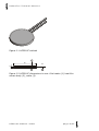
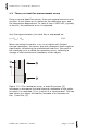
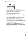
HFP01SC
Self Calibrating Heat Flux Sensortm
USER MANUAL
HFP01SC Manual v0811
Edited & Copyright by:
Hukseflux Thermal Sensors
http://www.hukseflux.com
e-mail: [email protected]
Hukseflux Thermal Sensors
Warning:
Putting more than 20 volts across the
heater of HFP01SC may result in
permanent damage to the sensor
HFP01SC Manual v0811
page 2/33
Hukseflux Thermal Sensors
Contents
List of symbols
Introduction
1
Theory of Self-Calibration
1.1 Introduction
1.2 Theory on heat flux measurement errors
1.3 Self-calibration
1.4 HFP01SC calculation
1.5 Additional quality assurance
2
Application in meteorology
3
Specifications of HFP01SC
4
Short user guide
5
Putting HFP01SC into operation
6
Installation of HFP01SC
7
Maintenance of HFP01SC
8
Requirements for data acquisition and control
9
Electrical connection of HFP01SC
10 Programming for HFP01SC
11 Appendices
11.1 Appendix on cable extension for HFP01SC
11.2 Appendix trouble shooting
11.3 CE declaration of conformity
HFP01SC Manual v0811
4
5
9
9
10
13
15
17
18
20
22
23
25
26
27
28
30
32
32
32
33
page 3/33
Hukseflux Thermal Sensors
List of symbols
Heat flux
Thermal conductivity
Voltage output
HFP01SC sensitivity (factory value)
HFP01SC sensitivity (newly found value)
Thermal conductivity dependence of Esen
Time
Surface area
Deflection error (+ when ϕ is overestimated)
Electrical resistance
Thermal resistance
Measurement at t is 0, 180 seconds
Difference before and during heating
ϕ
Wm-2
λ
W/m.K
V
V
μV/Wm-2
Esen
Esen2 μV/Wm-2
Eλ
mK/W
t
s
A
m2
X
%
R
Ω
Rth
Km2/W
(0), (180)
Δ
-
Subscripts
Property of thermopile sensor
Property of air
Property of the current sensing resistor
Properties of the heater for self test
Amplitude
Property during calibration
HFP01SC Manual v0811
sen
air
cur
self
amp
cal
page 4/33
Hukseflux Thermal Sensors
Introduction
The HFP01SC self-calibrating heat flux sensortm is a sensor
intended for high accuracy measurement of soil heat flux.
Also it offers improved quality assurance of the measurement.
The on-line calibration (the Van den Bos-Hoeksema method)
automatically corrects for various common errors, in particular
those due to the non-perfect matching of the thermal
conductivity of sensor and soil, and due to variations of the
thermal conductivity of the soil caused by varying moisture
content.
The self calibration can be used only if the sensor is completely
surrounded by at least 40 mm of the object.
A typical measurement location is equipped with 2 sensors for
good spatial averaging.
HFP01SC is a combination of a heat flux sensor and a film
heater. The primary purpose is to estimate the heat flux through
the surrounding soil. The HFP01SC output is a voltage signal that
is proportional heat flux through the sensor. The film heater that
is mounted on top can be activated to perform a calibration (see
chapter 1.3.), resulting in a new calibration factor that
compensates for the errors made under the circumstances of
that moment. Implicitly also cable connection, data acquisition
and data processing are tested. Also errors due to temperature
dependence and instability of the sensor are eliminated. The
result is a much improved accuracy & quality assurance of the
measurement (relative to conventional models such as model
HFP01).
The self-calibrating method has been developed at Hukseflux.
The main sensor of HFP01SC is a normal heat flux sensor.
The self calibration is performed by activating the film heater. It
is temporarily switched on to perform a heating cycle of around 3
minutes. During this cycle the normal heat flux measurement is
disabled.
HFP01SC Manual v0811
page 5/33
Hukseflux Thermal Sensors
The self calibration results in an improved sensitivity estimate for
the heat flux measurement. The HFP01SC design dates from
1998. In its first years of existence the HFP01SC has rapidly
been accepted as the state-of-the-art method for measurement
of soil heat flux in meteorology.
In meteorological applications there are two reasons for the
popularity of HFP01SC. The first reason is that it offers a higher
than usual level of accuracy, the second is that it offers a higher
than usual level of quality assurance of the measurement.
The accuracy of soil heat flux measurements very much depends
on the matching of the sensor thermal conductivity to that of the
surrounding medium. A typical heat flux sensor (Hukseflux
HFP01) has a thermal conductivity of 0.8 W/mK, while soils can
vary between extremes of 0.2 and 4 W/mK. Sand in relatively
dry condition can have a thermal conductivity of 0.3 W/mK
(perfectly dry 0.2) while the same sand when saturated with
water reaches 2.5 W/mK. A typical sensor performing a correct
measurement in dry sand will make a – 16% error in wet sand.
As in wet sand the heat tends to travel around the badly
conducting sensor, the flux will be underestimated by 16%.
This example serves to illustrate that in soils where conditions
vary the so-called “thermal conductivity dependence” leads to
large deflection errors.
The second important error is temperature dependence.
Over the entire temperature range from -30 to + 70 degrees C,
the temperature error is +/- 5%. Taking the worst case soil,
pure sand, for the conventional heat flux measurement in
meteorology the overall worst case accuracy is estimated to be
+8 /- 24%. This is rounded off to +10 / -25 %.
HFP01SC, by using the possibility to calibrate itself, eliminates
both errors. For the HFP01SC we estimate +/- 3%, which
essentially equals the initial calibration accuracy.
HFP01SC Manual v0811
page 6/33
Hukseflux Thermal Sensors
As for the Quality Assurance: measuring with a conventional
heat flux sensor, after the sensor is dug in it is assumed that its
remains where it is, in good contact with the soil, all cabling in
good condition. With the HFP01SC during the calibration
implicitly the cabling is checked, thermal connection and also the
soil thermal conductivity (as the correction that we make is
largely dependent on soil thermal conductivity).
Summarising: when compared to heat flux measurements with
conventional heat flux plates, measurement with HFP01SC has a
higher accuracy and by applying the measurement a better
quality accurance is achieved.
HFP01SC Manual v0811
page 7/33
Hukseflux Thermal Sensors
Figure 0.1 HFP01SC outlook
80
5m
5.0
Figure 0.2 HFP01SC dimensions in mm: film heater (1) heat flux
sensor body (2), cable (3).
HFP01SC Manual v0811
page 8/33
Hukseflux Thermal Sensors
1 Theory of Self-Calibration
1.1
Introduction
This chapter is written for users that are familiar with the general
theory of heat flux sensors and error sources in the heat flux
measurement. In case more information on this subject is
required, literature (most notably the HFP01 manual) is available
free of charge via e-mail as a PDF file. Please request at
[email protected].
The self calibrating principle can only be used if the sensor is
surrounded by at least 40 mm of soil. It is typically used in
meteorological applications for measurements of the soil heat
flux.
HFP01SC is a combination of a heat flux sensor and a film
heater. The heat flux sensor can, as usual, measure the heat flux
through the surrounding medium. The output is a voltage signal
that is proportional to the local heat flux.
This means that in case of emergency one can use HFP01SC as a
normal HFP01.
By activation of the heater, at reguar intervals an updated
calibration factor is determined.
Every new calibration results in an updated calibration factor
Esen2.
The main reasons for this update are changes in soil thermal
conductivity (deflection error) and temperature (temperature
dependence).
When performing this calibration, typically once every 3 or 6
hours (depending on available power), implicitly also cable
connection, data acquisition and data processing are tested.
Temperature dependence is eliminated. The result is a
dramatically improved accuracy & quality assurance of the
measurement (relative to using conventional sensors). The
method is generally referred to as the Van den Bos-Hoeksema
method.
More detailed explanation follows below.
HFP01SC Manual v0811
page 9/33
Hukseflux Thermal Sensors
1.2
Theory on heat flux measurement errors
Using a normal heat flux sensor, there are several common error
sources. In soil these are in particular the deflection error and
the temperatre dependence. In case of use of HFP01SC, typically
in the soil, the resistance error is neglected.
As a first approximation, the heat flux is expressed as:
ϕ = Vsen / Esen
1.2.1
When mounting the sensor in or on an object with limited
thermal resistance, the sensor thermal resistance itself might be
significantly influencing the undisturbed heat flux. One part of
the resulting error is called the resistance error, reflecting a
change of the total thermal resistance of the object.
Figure 1.2.1 The resistance error: a heat flux sensor (2)
increases or decreases the total thermal resistance of the object
on which it is mounted (1) or in which it is incorporated. This can
lead either to a larger of smaller (increase of or decrease of
the- ) heat flux (3).
HFP01SC Manual v0811
page 10/33
Hukseflux Thermal Sensors
Figure 1.2.2 The resistance error: a heat flux sensor (2)
increases or decreases the total thermal resistance of the object
on which it is mounted or in which it is incorporated. An
otherwise uniform flux (1) is locally disturbed (3).
A first order correction of the measurement is:
ϕ = (Rthobj+Rthsen ) V
sen
/E
sen
Rthobj
1.2.2
In addition to the resistance error, the fact that the medium
thermal conductivity differs from the sensor thermal conductivity
causes the heat flux to deflect. The resulting error is called the
deflection error. The deflection error is determined in media of
different thermal conductivity by experiments or using
theoretical approximations. The result of these experiments is
laid down as the so-called thermal conductivity dependence Eλ.
The order of magnitude of Eλ is constant for one sensor type. For
HFP01 and HFP01SC, Eλ is given in the list of specifications
Esen = E
sen, cal
(1+Eλ (λcal - λmed))
1.2.3
Note: this correction can only be applied when there is a
substantial amount of (at least 40 mm) medium on both sides of
the sensor. In soils λmed usually is not known. The value of λcal
typically is zero.
HFP01SC Manual v0811
page 11/33
Hukseflux Thermal Sensors
Figure 1.2.3 The deflection error. The heat flux (1) is deflected in
particular at the edges of the sensor. As a result the
measurement will contain an error; the so-called deflection error.
The magnitude of this error depends on the medium thermal
conductivity, sensor thermal properties as well as sensor design.
In addition, there is a temperature dependence TD reflects the
fact that the sensitivity changes with temperature:
Esen = E
sen, cal
(1+TD (Tcal - Tsen ))
1.2.4
Combining 1.2.3 and 1.2.4:
Esen =
E
sen, cal
{(1+Eλ (λcal - λmed))+ (1+TD (Tsen - Tcal ))} 1.2.5
Apart from the sensor's own thermal resistance, also contact
resistances between sensor and surrounding material are
demanding special attention. Essentially any air gaps add to the
sensor thermal resistance, at the same time increasing the
deflection error in an unpredictable way. In all cases the contact
between sensor and surrounding material should be as well and
as stable as possible, so that it is not influencing the
measurement. It should be noted that the conductivity of air is
approximately 0.02 W/m.K, ten times smaller than that of the
heat flux sensor. It follows that air gaps form major contact
resistances, and that avoiding the occurrence of significant air
gaps should be a priority whenever heat flux sensors are
installed.
HFP01SC Manual v0811
page 12/33
Hukseflux Thermal Sensors
1.3
Self-calibration
Figure 1.3.1 Explanation of the self-calibrating principle: On the
left the normal situation with a heat flux ϕ. Due to the fact that
sensor and medium do not match, the actual flux through the
sensor is reduced by a factor (1-X). This error is called deflection
error. On the right, the film heater that is mounted on top (1) is
activated to generate a well known heat flux ϕ. The response of
the heat flux sensor is measured. In the ideal situation 50% of
the generated flux ϕ would pass through the plate (typically 150
W/m2). In case of non matching thermal conductivities, a
deviation (X) will occur. The essence of this approach is that the
flow is divided in an upward flow through undisturbed medium
(1+X) and a downward flow through the heat flux sensor (a
disturbance) plus underlying medium. The (1-X) signal level
however, still represents a 0.5 ϕ heat flux level of the normal
situation of the picture on the left. In other words, the
comparison of the measured heat flux to the total artificially
generated heat flow is used to correct for the deflection error.
HFP01SC Manual v0811
page 13/33
Hukseflux Thermal Sensors
Figure 1.3.2 electrical connection HFP01SC. Sensor (2) wiring 1
and 2. Heater (1) heater voltage input wires 3 and 4. Heater
current measurement, typically performed by putting a 10 ohm
resistor (3) in series (not included with HFP01SC), and by
measuring the voltage across the resistor, wires 5 and 6. Dashed
line (4), sensor on the left and cable and datalogger on the right.
Figure 1.3.3 An alternative "short cut", explaining the working
principle of HFP01SC: in the self-calibrating heat flux plate, a
heater is incorporated. The reaction to a pulse in heating
represents the currently valid calibration constant. This principle
is valid in all environments, and eliminates errors due to the
thermal conductivity of the environment (soil moisture) and
temperature. In reality, the heat fluxes will deviate from 50%.
For calculation of the heat flux in the surrounding medium
however, the 50% -50% division remains valid.
HFP01SC Manual v0811
page 14/33
Hukseflux Thermal Sensors
1.4
HFP01SC calculation
The heater generally is switched on every three or six hours. The
totoal calibration takes about 6 minutes. During 3 of these 6
minutes, a current is lead through the film resistor for self test,
in order to generate a well-known heat flux. The sensor output
signal, Vsen, is measured. The difference in voltage output of the
sensor, Vamp, when heating and not heating multiplied by 2
(because only half of the flux passes the sensor) divided by the
heat flux, ϕsen, is the new sensor sensitivity, Esen2. Typically
measurements are done at 0, 180 and 360 seconds.
ϕsen = (V2cur.Rself) / (R2cur.Aself)
1.4.1
Vamp
1.4.2
= ABS [ {Vsen (0) + Vsen (360)}/2 - Vsen (180) ]
ABS stands for the absolute value.
Esen2 = 2Vamp / ϕsen
1.4.3
Concluding:
Esen 2 = 2Vamp (R2cur.Aself)/(V2cur.Rself)
1.4.4
For HFP01SC’s heater a typical value is Aself =38.85 10-4 m2, an
Rcur is recommended 10 Ω and an Rself is sensor specific, around
100Ω. With the mentioned values ϕsen = 257.V2cur. Please mind
that Vcur in this case is about 0.1 times the voltage that is
applied across the total circuit. At a 12-Volt power supply, Vcur
would be 1.09 Volt; the heat flux would be 305 W/m2, half of
which would pass the heat flux sensor. Power would be around
0.02 Watt (when switched on every 3 hours).
For type HFP01SC with Rcur of 10 Ω and an Rself of 100Ω :
Esen2 = Vamp / 129 V2cur
1.4.5
The soil heat flux is calculated as:
ϕ = Vsen / Esen2
HFP01SC Manual v0811
1.4.6
page 15/33
Hukseflux Thermal Sensors
The factory delivered calibration factor Esen is determined at the
factory using an electrically generated heat flux that is forced
through the sensor.
In soils, corrections of up to +5 to -20% relative to the factory
supplied calibration coefficient can be expected. (the +5% due to
temperature dependence)
During the calibration process it is suggested to discard the
measured values of the heat flux. This implies that during 6
minutes one could copy the flux value of just before the
calibration.
In case very small flux levels are measured, a delay of 10 mintes
can be used.
HFP01SC Manual v0811
page 16/33
Hukseflux Thermal Sensors
1.5
Additional quality assurance
If possible, additional measures for quality assurance of the
measurement can be programmed.
It is suggested to generate an error message if Esen2 is larger
than the factory delivered Esen by more than 5%, and smaller by
more than 20%.
A possible error source is that there has been too much
fluctuation between of the heat flux in the soil during the
calibration process. As a limit we suggest to allow the
measurements at t = 0 and t = 180 to differ no more than 10 %
of the signal amplitude during calibration Vamp of formula 2.
Summarising: possible quality checks:
1: Esen2 < 0.8 Esen
2: Esen2 > 1.05 Esen
3: Vsen (0) - Vsen (360) < 0.1 Vamp
HFP01SC Manual v0811
page 17/33
Hukseflux Thermal Sensors
2 Application in meteorology
In meteorological applications the primary purpose is to measure
the part of the energy balance that goes into the soil. This soil
heat flux in itself is in most cases of limited interest. However,
knowing this quantity, it is possible to “close the balance". In
other words, apply the law of conservation of energy to check
the quality of the other (convective and evaporative) flux
measurements. For more information on meteorological
measurement of heat flux, see the appendix.
The soil heat flux measurement with HFP01SC is the most
accurate solution available.
Figure 2.1 Typical meteorological energy balance measurement
system with HFP01SC (typically 2 pieces) installed under the soil.
In addition to the measurement errors mentioned in the
introduction, the heat flux measurement in meteorology suffers
from the fact that it is spatially variable.
In field experiments it is difficult to find one location that can be
considered to be representative of the whole region. Also
temporal effects of shading on the soil surface can give a false
impression of the heat flux. For this reason typically two sensors
are used for each station, usually at a distance of 5 meters.
HFP01SC Manual v0811
page 18/33
Hukseflux Thermal Sensors
Heat flux sensors in meteorological applications are typically
buried at a depth of about 5 cm below the soil surface.
Burial at a depth of less than 5 cm is generally not
recommended. In most cases a 5 cm soil layer on top of the
sensor offers just sufficient mechanical consistency to guarantee
long-term stable installation conditions.
Burial at a depth of more than 8 cm is generally not
recommended, because time delay and amplitude become less
easily traceable to surface fluxes at larger installation depths.
See the appendix for more details.
HFP01SC Manual v0811
page 19/33
Hukseflux Thermal Sensors
3 Specifications of HFP01SC
HFP01SC self-calibrating heat flux sensor is intended to be used
for determining the heat flux in soil. It is normally used in
combination with a suitable measurement and control system,
including power supply and relay to activate the self calibration
process.
HFP01SC GENERAL SPECIFICATIONS
Specified
Heat flux in W/m2 perpendicular to the
measurements
sensor surface
Installation
See the product manual for
recommendations.
Temperature range
-30 to +70 degrees C
Recommended number Meteorological: two for each
of sensors
measurement station.
CE requirements
HFP01SC complies with CE directives
Required depth of
The medium must be all around
insertion
HFP01SC in good thermal contact. The
sensor must be below the surface for at
least 40 mm, typically 50 mm
HFP01SC MEASUREMENT SPECIFICATIONS
Expected accuracy
+/- 3% (heat flux measurements)
Overall uncertainty
estimated to be within +5 /- 5%, based
statement according to on a standard uncertainty multiplied by
ISO
a coverage factor of k = 2, providing a
level of confidence of 95%.
This is a statement according to ISO,
and is according to the manufacturer
too pessimistic.
Thermal conductivity
-0.07 % m.K/W (nominal value)
compensated during self-calibration
dependence Eλ
Temperature
< 0.1%/ °C
dependence TD
compensated during self-calibration
HFP01SC SENSOR SPECIFICATIONS
Esen (nominal)
50 µV/ W. m-2 (exact value on
calibration certificate)
λcal = 0, Tcal =20 °C
Esen is adapted during self-calibration
Sensor thermal
0.8 W/mK
conductivity
Sensor thermal
< 6.25 10 -3 Km2/W
resistance Rth
Table 3.1 List of HFP01SC specifications. (continued on the next
page)
HFP01SC Manual v0811
page 20/33
Hukseflux Thermal Sensors
Response time
(nominal)
Range
Non stability
± 3 min (equals average soil)
+ 2000 to - 2000 W.m-2
< 1% change per year (normal
meteorological use)
compensated during self-calibration
Required readout /
1.1 one differential voltage channel
hardware
or possibly (less ideal)
1.2 one single ended voltage channel.
When using more than one sensor and
having a lack of input channels, it can
be considered to put several sensors in
series, while working with the average
sensitivity.
2 one current measurement (typically
realised using a voltage measurement
across a 10 ohm resistor.
3 one Relay and timer to switch 12V,
0.1 A power to the heater.
Expected voltage
Meteorology: -10 to 20 mV (sensor),
output
0 to 2 V (heater current measuerment)
Heater resistance, area 90 - 110 ohm, 0.003885 m2
Voltage input (heater) 9-15 VDC (nominal), switched
Sensor resistance
2 Ohm (nominal) plus cable resistance
Heating power
1.5 W typically during 180 s, typically
every 3 or 6 hours
Power consumption
Average 0.02 (3 hr) or 0.04 (6hr) W
Required programming ϕ = Vsen/ Esen
Sensor dimensions
80 mm diameter, 5 mm thickness
Cable length, diameter 5 meters, 5 mm, 2 cables
Weight including 5 m
0.3 kg
cable, transport dim.
transport dimensions 32x23x3 cm
CALIBRATION
Calibration traceability to the “guarded hot plate” of National
Physical Laboratory (NPL) of the UK.
Applicable standards are ISO 8302 and
ASTM C177.
Recalibration interval
Not applicable
OPTIONS
Extended cable
Additional cable length x metres (add to
5m)
Table 4.1 List of HFP01SC specifications. (started on previous
page)
HFP01SC Manual v0811
page 21/33
Hukseflux Thermal Sensors
4 Short user guide
Preferably one should read the introduction and the section on
theory. Really important items are put in boxes.
The sensor should be installed following the directions of the
next paragraphs. Essentially this requires a data logger and
control system capable of switching, readout of voltages, and
capability to perform calculations based on the measurement.
The first step that is described in paragraph 5 is and indoor test.
The purpose of this test is to see if the system works. It can be
done in a very simple way.
The second step is to make a final system set-up. This is
strongly application dependent, but it usually involves complete
programming and automation of the system.
Directions for this can be found in paragraphs 6 to 12.
HFP01SC Manual v0811
page 22/33
Hukseflux Thermal Sensors
5 Putting HFP01SC into operation
It is recommended to test the sensor functionality by checking
the impedance of the sensor and heater, and by checking if the
sensor works, according to the following table: (estimated time
needed: 20 minutes)
Check the connection of the heater. Use
a multimeter at the 200 ohms range.
Measure between two wires that are
connected to the heater. The typical
impedance of the wiring is 0.1 ohm/m.
Typical impedance should be 1.5 ohm
for the total resistance of two wires
(back and forth) of each 5 meters, plus
the heater resistance that is indicated
on the calibration certificate.
Warning: during this part of the test,
please put the sensor in a thermally
quiet surrounding because a sensor that
generates a significant signal will
disturb the measurement.
Infinite indicates a
broken circuit; zero
indicates a short circuit.
Expected value around
110 Ohms.
The typical impedance
of the wiring is 0.1
ohm/m. Typical
impedance should be
1.5 ohm for the total
resistance of two wires
Check the impedance of the sensor. Use (back and forth) of
each 5 meters, plus the
a multimeter at the 10 ohms range.
Measure at the sensor output first with typical sensor
one polarity, than reverse polarity. Take impedance of between
2 and 5 ohms. Infinite
the average value.
indicates a broken
circuit; zero indicates a
short circuit.
Check if the sensor reacts to heat flux. The thermopile should
Use a multimeter at the millivolt range. react by generating a
Measure at the sensor output. Generate millivolt output signal.
a signal by touching the thermopile hot
joints (red side) with your hand.
If possible put a voltage to the heater
The thermopile should
between 9 and 12 Volt to see the heater react by generating a
functionality.
millivolt output signal.
Table 5.1 Checking the functionality of the sensor. The procedure
offers a simple test to get a better feeling how HFP01SC works,
and a check if the sensor is OK.
HFP01SC Manual v0811
page 23/33
Hukseflux Thermal Sensors
The HFP01SC should be connected to the measurement and
control system as described in the chapter on the electrical
connection.
The programming of data loggers is the responsibility of the
user. Please contact the supplier to see if directions for use with
your system are available.
HFP01SC Manual v0811
page 24/33
Hukseflux Thermal Sensors
6 Installation of HFP01SC
HFP01SC is generally installed at the location where one wants
to measure at least 4 cm depth below the surface. A typical
depth of installation is 5 cm.
Typically 2 sensors are used per measurement location in order
to promote spatial averaging, and to have some redundancy for
improved quality assurance. Sensors are typically several
meters apart.
The more even the surface on which HFP01SC is placed the
better. When covering HFP01SC with the medium, it should be
done such that the medium below and on top is the same.
Usually this means that it is safest either to install HFP01SC
from the side. When installing by digging a hole, it is
recommended to dig the hole some 40 mm deeper than the
location of HFP01SC so that eventually the disturbance of the
soil is the same above and below the sensor.
For the self-calibrating principle to work properly, the sensor
must be installed at least for 40 mm below the surface.
In meteorological applications, permanent installation is
preferred. It is recommended to fix the location of the sensor
by attaching a metal pin to the cable. Attachment of the pin to
the cable can be done using a tie-wrap.
Table 6.1 General rules for installation of HFP01SC. In case of
exceptional applications, please contact Hukseflux.
HFP01SC Manual v0811
page 25/33
Hukseflux Thermal Sensors
7 Maintenance of HFP01SC
Once installed, HFP01SC is essentially maintenance free. Usually
errors in functionality will appear as unreasonably large or small
measured values.
As a general rule, this means that a critical review of the
measured data is the best form of maintenance.
In case 2 sensors are mounted on one location the ratio of
measurement resuls could be monitored over time; this will give
a clue if there is any unstability.
At regular intervals the quality of the cables can be checked.
On a 2 yearly interval the calibration can be checked in an indoor
facility.
HFP01SC Manual v0811
page 26/33
Hukseflux Thermal Sensors
8 Requirements for data
acquisition and control
Capability to measure
microvolt signals (sensor
signal)
Capability of measuring
currents
Capability of switching
Requirements for power
supply of the heater
Capability for the data logger
or the software
5 microvolt resolution or better
Around 0.1A, with 1% accuracy,
typicaly perfromed by using a 10
Ohm resistor and measurement
of the voltage across this
resistor.
9-15 volt at 0.1 A (this is for one
sensor only, worst case)
Capability to supply 9-15 Volt, at
0.1 A
In meteorological applications,
this is typically done for 3
minutes every three or six
hours, depending on the
available power.
The average required power
across the day in this case is
0,02 and 0.04 Watt respectively.
To store data, to subtract and to
perform the calculations.
Table 8.1 Requirements for data acquisition and control.
HFP01SC Manual v0811
page 27/33
Hukseflux Thermal Sensors
9 Electrical connection of
HFP01SC
In order to operate, HFP01SC should be connected to a
measurement and control system as described above. A typical
connection is shown in figure 9.1. For the purpose of making a
correct measurement of the heater power there is a current
sensing resistor in the wire that leads to the heater. The voltage
over a 10-ohm current sensing resistor should be of the order of
magnitude of 1 to 2 Volts. The required resistance must be
0.1%, 50ppm or better. We recommend to use a value of 10
ohm, 0.1%, 50ppm, 0.6 Watt or similar.
Figure 9.1 electrical connection HFP01SC. Sensor (2) wiring 1
and 2. Heater (1) heater voltage input wires 3 and 4. Heater
current measurement, typically performed by putting a 10 ohm
resistor (3) in series, and by measuring the voltage across the
resistor, wires 5 and 6. Dashed line (4), sensor on the left and
cable and datalogger on the right.
A relay should be used to switch the heater on and off. The heat
flux plate output usually is connected to a differential voltage
input. The voltage across the current sensing resistor is also
measured by a differential voltage channel. HFP01SC has two
separate cables, one for the signal and one for the heater. The
colour codes can be found on the calibration certificate.
NOTE: the resistor is normally not part of the delivery.
HFP01SC Manual v0811
page 28/33
Hukseflux Thermal Sensors
Wire colour code
Heat flux sensor +
White
Heat flux sensor Green
Heater
Brown
Heater
Green
Table 9.1 typical HFP01SC colour code
Cable Number
1
1
2
2
NOTE: Sensors suplied by Campbell Scientific USA sually have a
diferent wiring diagram; see the Campbell manual for ore
information. In most cases the 10 ohm is included into th sensor
wiring.
Warning:
Putting more than 20 volt across the heater may result in
permanent damage to the sensor
HFP01SC Manual v0811
page 29/33
Hukseflux Thermal Sensors
10 Programming for HFP01SC
The central formula is:
Esen 2 = 2Vamp (R2cur.Aself)/(V2cur.Rself)
1.4.4
Rself and Aself are given on the sensor calibration certificate. Rcur
is user supplied.
The soil heat flux is calculated as:
ϕ =V
sen
/E
sen2
1.4.6
Possible quality assurance tests are:
1: Esen2 < 0.8 Esen
2: Esen2 > 1.05 Esen
3: Vsen (0) - Vsen (360) < 0.1 Vamp
In case the heater is not connected, one can work with HFP01SC
as if it were a normal heat flux plate, using formula 1.4.6 in
combination with Esen as supplied on the sensor calibration
certificate.
HFP01SC Manual v0811
page 30/33
Hukseflux Thermal Sensors
Sensor
specific
part,
entering
Rself, Rcur
and Aself,
possibly
also Esen.
Repetitive
loop
typically 3
or 6 hour
repetition.
This is typically done in the
data logger, but could also be
done in a later stage, during
processing.
The heater
resistance, Aself and
Esen can be found on
the calibration
certificate.
Measure Vsen(0)
Store Vsen(0)
There usually will be
a significant signal
representing the
present heat flux at
that moment.
Typically for 6
minutes, can also
be stoped for
longer.
Temporarily stop the normal
soil heat flux measurement
Switch heater on
Measure the voltage across
the current sensing resistor
Vcur
Measure the steady state
sensor output Vsen(180).
Store Vsen(180).
Switch off the heater
Measure the steady state
sensor output Vsen(360).
Store Vsen(360).
Calculate the average of
Vsen(0) and Vsen(360).
This is to
compensate for
changes in soil heat
flux level.
Calculate the amplitude Vamp.
Calculate the new sensor Esen2
Do quality assurance tests
Start normal soil heat flux
measurement again using
Esen2
Repeat either on user demand
or on a regular time schedule
Table 10.1 Typical ingredients of a program for measurement
and control of HFP01SC.
HFP01SC Manual v0811
page 31/33
Hukseflux Thermal Sensors
11 Appendices
11.1 Appendix on cable extension for HFP01SC
HFP01SC has 2 cables, one for the sensor, and one for the
heater.
It is a general recommendation to keep the distance between
data logger and sensor as short as possible. Cables generally act
as a source of distortion, by picking up capacitive noise.
HFP01SC cable can however be extended without any problem to
100 meters. If done properly, the sensor signal, although small,
will not degrade because the sensor impedance is very low. Also
connection of the heater is immune to cable extension.
Cable and connection specifications are summarised below.
Cable:
2-wire shielded, copper core (at Hukseflux we use 3
wire shielded, of which we only use 2 per cable)
0.1 Ω/m or lower
Core
resistance
Outer
(preferred) 5 mm
diameter
Outer sheet (preferred) polyurethane (for good stability in
outdoor applications).
Connection Either solder the new cable core and shield to the
original sensor cable, and make a waterproof
connection, or use gold plated waterproof
connectors.
Table 11.1.1 Specifications for cable extension of HFP01SC
11.2 Appendix trouble shooting
This paragraph contains information that can be used to make a
diagnosis whenever the sensor does not function.
It is recommended to start any kind of trouble shooting with a
simple check of the sensor and heater impedance. This test can
be found in chapter 5. The advantage of this test is that it can be
done even if the sensor is dug in.
The second thing to do is a check to see if the thermopile gives a
signal. The suggestion is to take a 9-15 Volt battery and to put it
across the wires leading to the heater. If these tests still did not
give any clue, please contact the supplier.
HFP01SC Manual v0811
page 32/33
Hukseflux Thermal Sensors
11.3 CE declaration of conformity
According to EC guidelines 89/336/EEC, 73/23/EEC and
93/68/EEC
We:
Hukseflux Thermal Sensors
Declare that the product:
HFP01SC
Is in conformity with the following standards:
Emissions:
Radiated:
Conducted:
EN 55022: 1987
EN 55022: 1987
Immunity:
ESD IEC 801-2; 1984
RF IEC 808-3; 1984
EFT IEC 801-4; 1988
Class A
Class B
8kV air discharge
3 V/m, 27-500 MHz
1 kV mains, 500V other
Delft,
January 2006
HFP01SC Manual v0811
page 33/33