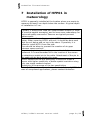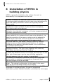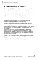
1
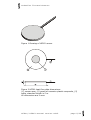
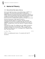
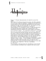
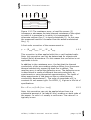
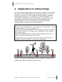
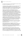
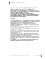
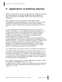
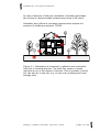
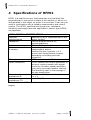
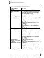
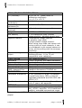
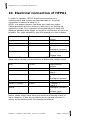
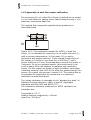
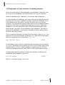
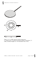
HFP01 & HFP03
Heat Flux Plate
Heat Flux Sensor
USER MANUAL
HFP01/ HFP03 manual version 0612
Edited & Copyright by:
Hukseflux Thermal Sensors
http://www.hukseflux.com
e-mail: [email protected]
Hukseflux Thermal Sensors
Contents
1
1.1
1.2
2
3
4
5
6
7
8
9
10
11
11.1
11.2
11.3
11.4
11.5
11.6
11.7
List of symbols
4
Introduction
5
General Theory
6
General heat flux sensor theory
6
Detailed description of the measurement: resistance error,
contact resistance, deflection error and temperature
dependence
8
Application in meteorology
11
Application in building physics
14
Specifications of HFP01
16
Short user guide
19
Putting HFP01 into operation
20
Installation of HFP01 in meteorology
21
Installation of HFP01 in building physics
22
Maintenance of HFP01
24
Electrical connection of HFP01
26
Appendices
27
Appendix on cable extension for HFP01
27
Appendix on trouble shooting
28
Appendix on heat flux sensor calibration
29
Appendix on heat transfer in meteorology
30
Appendix on heat transfer in building physics
32
Appendix on HFP03
33
CE declaration of conformity
35
HFP01/ HFP03 manual version 0612
page 2/35
Hukseflux Thermal Sensors
List of symbols
Heat flux
Thermal conductivity of the
surrounding medium or object on which
the sensor is mounted
Voltage output
HFP01 sensitivity
Thermal conductivity dependence of Esen
Time
Surface area
Electrical resistance
Thermal resistance
Temperature
Temperature dependence
Depth of burial
ϕ
W m-2
λ
V
Esen
Eλ
t
A
Re
Rth
T
TD
d
W/mK
V
µV/Wm-2
mK/W
s
m2
Ω
Km2/W
K
%/K
m
Subscripts
Property of the sensor
Property of air
Property during calibration
Property of the object on which HFP01 is
mounted
Property at the soil surface
HFP01/ HFP03 manual version 0612
sen
air
cal
obj
surf
page 3/35
Hukseflux Thermal Sensors
Introduction
HFP01 is the world’s most popular sensor for heat flux
measurement in the soil and through walls and building
envelopes. By using a ceramics-plastic composite body the total
thermal resistance is kept small.
HFP01 serves to measure the heat that flows through the object
in which it is incorporated or on which it is mounted. The actual
sensor in HFP01 is a thermopile. This thermopile measures the
differential temperature across the ceramics-plastic composite
body of HFP01. Working completely passive, HFP01 generates a
small output voltage proportional to the local heat flux.
Using HFP01 is easy. For readout one only needs an accurate
voltmeter that works in the millivolt range. To calculate the heat
flux, the voltage must be divided by the sensitivity; a constant
that is supplied with each individual instrument.
HFP01 can be used for in-situ measurement of building envelope
thermal resistance (R-value) and thermal transmittance (Hvalue) according to ISO 9869, ASTM C1046 and ASTM 1155
standards.
Traceability of calibration is to the “guarded hot plate” of
National Physical Laboratory (NPL) of the UK, according to ISO
8302 and ASTM C177.
A typical measurement location is equipped with 2 sensors for
good spatial averaging. If necessary two sensors can be put in
series, creating a single output signal.
If measuring in soil, in case a more accurate measurement is
needed the model HFP01SC should be considered.
In case a more sensitive measurement is required, model HFP03
should be considered.
In case of special requirements, like high temperature limits,
smaller size or flexibility the PU series could offer a solution.
This manual can also be used for HFP03. Differences between
HFP03 and HFP01 are highlighted in a special appendix on
HFP03.
HFP01/ HFP03 manual version 0612
page 4/35
Hukseflux Thermal Sensors
Figure 1 Drawing of HFP01 sensor
Figure 2 HFP01 heat flux plate dimensions:
(1) sensor area, (2) guard of ceramics-plastic composite, (3)
cable, standard length is 5 m.
All dimensions are in mm.
HFP01/ HFP03 manual version 0612
page 5/35
Hukseflux Thermal Sensors
1 General Theory
1.1
General heat flux sensor theory
As in most heat flux sensors, the actual sensor in HFP01 is a
thermopile. This thermopile measures the differential
temperature across the ceramics-plastic composite body of
HFP01. Working completely passive, it generates a small output
voltage that is proportional to the differential temperature that
powers the heat flux travelling through it. (heat flux is
proportional to the differential temperature divided by the local
thermal conductivity of the heat flux sensor).
Assuming that the heat flux is steady, that the thermal
conductivity of the body is constant and that the sensor has
negligible influence on the thermal flow pattern, the signal of
HFP01 is proportional to the local heat flux in Watt per square
meter.
Using HFP01 is easy. For readout one only needs an accurate
voltmeter that works in the millivolt range. To convert the
measured voltage Vsen to a heat flux ϕ, the voltage must be
divided by the sensitivity Esen, a constant that is supplied with
each individual sensor.
ϕ = Vsen / Esen
1.1.1
HFP01 is a weatherproof sensor. It complies with the CE
directives.
HFP01/ HFP03 manual version 0612
page 6/35
Hukseflux Thermal Sensors
Figure 1.1 General characteristics of a heat flux sensor like
HFP01.
When heat (6) is flowing through the sensor, the filling material
(3) will act as a thermal resistance. Consequently the heat flow ϕ
will go together with a temperature gradient across the sensor,
creating a hot side (5) and a cold side (4). The majority of heat
flux sensors is based on a thermopile; a number of
thermocouples (1,2) connected in series. A single thermocouple
will generate an output voltage that is proportional to the
temperature difference between the joints (copper-constantan
and constantan-copper). This temperature difference is, provided
that errors are avoided, proportional to the heat flux, depending
only on the thickness and the average thermal conductivity of
the sensor. Using more thermocouples in series will enhance the
output signal. In the picture the joints of a copper-constantan
thermopile are alternatively placed on the hot- and the cold side
of the sensor. The two different alloys are represented in
different colours 1 and 2. The thermopile is embedded in a filling
material, usually a plastic, in case of HFP01 a special Ceramicsplastic composite. Each individual sensor will have its own
sensitivity, Esen, usually expressed in Volts output, Vsen, per Watt
per square meter heat flux ϕ. The flux is calculated:
ϕ = Vsen/ Esen.
The sensitivity is determined at the manufacturer, and is found
on the calibration certificate that is supplied with each sensor.
HFP01/ HFP03 manual version 0612
page 7/35
Hukseflux Thermal Sensors
1.2
Detailed description of the measurement: resistance
error, contact resistance, deflection error and
temperature dependence
As a first approximation, the heat flux is expressed as:
ϕ = Vsen / Esen
1.2.1
This paragraph offers a more detailed description of the heat flux
measurement. It should be noted that the following theory for
correcting deflection errors and temperature dependence is not
often applied. Usually one will work with formula 1.2.1, possibly
corrected with 1.2.2.
When mounting the sensor in or on an object with limited
thermal resistance, the sensor thermal resistance itself might be
significantly influencing the undisturbed heat flux. One part of
the resulting error is called the resistance error, reflecting a
change of the total thermal resistance of the object.
Figure 1.2.1 The resistance error: a heat flux sensor (2)
increases or decreases the total thermal resistance of the object
on which it is mounted (1) or in which it is incorporated. This can
lead either to a larger of smaller (increase of or decrease of
the- ) heat flux (3).
HFP01/ HFP03 manual version 0612
page 8/35
Hukseflux Thermal Sensors
Figure 1.2.2 The resistance error: a heat flux sensor (2)
increases or decreases the total thermal resistance of the object
on which it is mounted or in which it is incorporated. An
otherwise uniform flux (1) is locally disturbed (3). In this case
the measured heat flux is smaller than the actual undisturbed
flux,( 1).
A first order correction of the measurement is:
ϕ = (Rthobj+Rthsen ) V
sen
/E
sen
Rthobj
1.2.2
This correction is often applied with thin or well-isolated walls.
Note: this correction can only be determined for objects with
limited (finite) dimensions. For this reason this correction is not
applicable in soils.
In addition to the resistance error, the fact that the thermal
conductivity of the surrounding medium differs from the sensor
thermal conductivity causes the heat flux to deflect. The
resulting error is called the deflection error. The deflection error
is determined in media of different thermal conductivity by
experiments or using theoretical approximations. The result of
these experiments is laid down as the so-called thermal
conductivity dependence Eλ. The order of magnitude of Eλ is
constant for one sensor type. For HFP01, Eλ is given in the list of
specifications.
Esen = E
sen, cal
(1+Eλ (λcal - λmed))
1.2.3
Note: this correction can only be applied when there is a
substantial amount of (at least 40 mm) medium on both sides of
the sensor. In soils λmed usually is not known. The value of λcal
typically is zero.
HFP01/ HFP03 manual version 0612
page 9/35
Hukseflux Thermal Sensors
Figure 1.2.3 The deflection error. The heat flux (1) is deflected in
particular at the edges of the sensor. As a result the
measurement will contain an error; the so-called deflection error.
The magnitude of this error depends on the medium thermal
conductivity, sensor thermal properties as well as sensor design.
In addition, the sensitivity of heat flux sensors is temperature
dependent. The temperatre dependence TD reflects the fact that
the sensitivity changes with temperature:
Esen = E
sen, cal
(1+TD (Tcal - Tsen ))
1.2.4
Combining 1.2.3 and 1.2.4:
Esen =
E
sen, cal
{(1+Eλ (λcal - λmed))+ (1+TD (Tsen - Tcal ))}
1.2.5
This correction is rarely applied because TD is typically small.
Apart from the sensor's own thermal resistance, also contact
resistances between sensor and surrounding material are
demanding special attention. Essentially any air gaps add to the
sensor thermal resistance, at the same time increasing the
deflection error in an unpredictable way. In all cases the contact
between sensor and surrounding material should be as well and
as stable as possible, so that it is not influencing the
measurement. It should be noted that the conductivity of air is
approximately 0.02 W/m.K, ten times smaller than that of the
heat flux sensor. It follows that air gaps form major contact
resistances, and that avoiding the occurrence of significant air
gaps should be a priority whenever heat flux sensors are
installed.
HFP01/ HFP03 manual version 0612
page 10/35
Hukseflux Thermal Sensors
2 Application in meteorology
In meteorological applications the primary purpose is to measure
the part of the energy balance that goes into the soil. This soil
heat flux in itself is in most cases of limited interest. However,
knowing this quantity, it is possible to “close the balance". In
other words, apply the law of conservation of energy to check
the quality of the other (convective and evaporative) flux
measurements. For more information on meteorological
measurement of heat flux, see the appendix.
Users should be aware of the fact that the soil heat flux
measurement with HFP01 in most cases is not resulting in a high
accuracy result. The main causes are:
1 the fact that measurement at one location in the soil will have
only limited validity for a larger area; variability of soil surface
can be very lage.
2 the fact that variations in soil thermal properties over time
result in significant measurement errors.
If measuring in soil, in case a more accurate measurement is
needed the model HFP01SC should be considered.
Figure 2.1 Typical meteorological energy balance measurement
system with HFP01 installed under the soil.
HFP01/ HFP03 manual version 0612
page 11/35
Hukseflux Thermal Sensors
In a perfect environment, the initial calibration accuracy of heat
flux sensors is estimated to be +3 /- 3%.
In field experiments it is difficult to find one location that can be
considered to be representative of the whole region. Also
temporal effects of shading on the soil surface can give a false
impression of the heat flux. For this reason typically two sensors
are used for each station, usually at a distance of 5 meters.
Apart from the question of representativeness of the
measurement location, the main problem with heat flux
measurements in meteorology is that the sensitivity of a heat
flux sensor is dependent on the thermal conductivity of the
surrounding medium. This deflection error is described in chapter
1. In soil heat flux measurement the accuracy of soil heat flux
measurements very much suffers from the fact that the
surrounding medium is both unknown to the manufacturer and
changing over time. A typical HFP01 has a thermal conductivity
of 0.8 W/mK, while soils can vary between extremes of 0.2 and
4 W/mK. Sand in relatively dry condition can have a thermal
conductivity of 0.3 W/mK (perfectly dry 0.2) while the same
sand when saturated with water reaches 2.5 W/mK. A typical
HFP01 performing a correct measurement in dry sand will make
a – 16% error in wet sand. As in wet sand the heat tends to
travel around the badly conducting sensor, the flux will be
underestimated by 16%.
This example serves to illustrate that in soils where conditions
vary the so-called thermal conductivity dependence leads to
large deflection errors.
The third important error is temperature dependence.
Over the entire temperature range from -30 to + 70 degrees C,
the temperature error is +/- 5%. Taking the worst case soil,
pure sand, for the conventional heat flux measurement in
meteorology the overall worst case accuracy is estimated to be
+8 /- 24%. This is rounded off to +10 / -25 %.
In most situations the soil will not be pure sand, and in an
average climate the difference between the yearly extremes
might be -10 + 40 degrees C and a thermal conductivity range
from 0.2 to 1 W/mK. The temperature error then is +2 / -3%,
the thermal conductivity accounts for +0 / - 7%, the calibration
+3 / -3 %. The result of +5 / -13 % is rounded off to +5 / -15%
HFP01/ HFP03 manual version 0612
page 12/35
Hukseflux Thermal Sensors
Heat flux sensors in meteorological applications are typically
buried at a depth of about 5 cm below the soil surface.
Burial at a depth of less than 5 cm is generally not
recommended. In most cases a 5 cm soil layer on top of the
sensor offers just sufficient mechanical consistency to guarantee
long-term stable installation conditions.
Burial at a depth of more than 8 cm is generally not
recommended, because time delay and amplitude become less
easily traceable to surface fluxes at larger installation depths.
See the appendix for more details.
Summary:
In case of use of HFP01 in meteorological applications, the use of
2 sensors per station is recommended. This creates redundancy
and a better possiblity for judging the quality of the
measurement accuracy. Typically one will work with two
separately measured sensor outputs; the average value is the
measurement result.
In normal soils (clays, silts) the overall expected measurement
accuracy for 12 hr totals is +5 / -15%.
In case of pure sands the overall measurement accuracy for 12
hr totals is +10 / -25 %.
The accuracy mainly is a function of the thermal conductivity of
the surrounding medium. In case of soils the moisture content
plays a dominant role.
The wider accuracy range in sand is due to the fact that the
thermal conductivity of sand varies with moisture content from
roughly 0.2 (perfectly dry) to 2.5 (saturated).
With other soils and walls (see chapter on building physics) the
variation of thermal conductivity is much less; roughly from 0.1
to 1 W/mK.
If measuring in soil, in case a more accurate measurement is
needed the model HFP01SC should be considered.
HFP01/ HFP03 manual version 0612
page 13/35
Hukseflux Thermal Sensors
3 Application in building physics
HFP01 can be used for in-situ measurement of building envelope
thermal resistance (R-value) and thermal transmittance (Hvalue) according to ISO 9869, ASTM C1046 and ASTM 1155
standards.
When studying the energy balance of buildings, heat is
exchanged by various mechanisms. The total result is a certain
heat flux. The dominant mechanisms are usually radiative
transfer by solar radiation and convective transport by flowing
air.
In most applications in building physics the sensor HFP01 is
simply mounted on or in the object of interest (see figure 3.1).
At the sensor surface, the convective heat of the air and the
radiation by the sun are transformed into conductive heat.
In case of incorporation into the wall, the conductive flux
through the wall is directly measured.
If direct beam solar radiation is present, the solar radiation is
usually dominant. The maximum expected solar radiation level is
about 1500 W/m2. In case of convective transport of heat by the
air, the convective transport is roughly proportional to the
difference in temperature between wall and air, and strongly
depends on the local wind speed. See the appendix on heat
transfer in building physics for more information.
It is possible that the heat flux sensor contributes significantly to
the total thermal resistance of the object (resistance error). In
this case the heat flux measurement must be corrected. For the
correction, see chapter 1. In order to limit the resistance error,
in all cases the contact between sensor and surrounding material
should be as well and as stable as possible, so that air gaps are
not influencing the measurement.
In a perfect environment, the initial calibration accuracy of heat
flux sensors is estimated to be +3 /- 3%.
In case of use of HFP01 on walls (insulating as well as bricks and
cements) the overall expected measurement accuracy for 12 hr
totals is +5 / -5 %.
HFP01/ HFP03 manual version 0612
page 14/35
Hukseflux Thermal Sensors
In case of analysis of thermal resistance of building envelopes,
the minimum recommended measurement time is 48 hours.
Hukseflux also offeres a complete measurement system for
analysis of building envelopes: TRSYS.
Figure 3.1 Estimation of convective, radiative and conductive
heat flux in building physics. The heat flux sensor is simply
mounted on or in the object of interest. This is typically in walls,
but can also be in the soil, e.g. on top of an underground heat
storage tank.
HFP01/ HFP03 manual version 0612
page 15/35
Hukseflux Thermal Sensors
4 Specifications of HFP01
HFP01 is a heat flux sensor that measures the local heat flux
perpendicular to the sensor surface in the medium in which it is
incorporated or the object on which it is mounted. It can only be
used in combination with a suitable measurement and control
system. The HFP01 specifications except size, resistance,
sensitivity and weight are also applicable to sensor type HFP03;
see appendix.
HFP01 GENERAL SPECIFICATIONS
Specified
Heat flux in W/m2 perpendicular to the
measurements
sensor surface
Installation
See the product manual for
recommendations.
Temperature range
-30 to +70 degrees C
Recommended number Meteorological: two for each
of sensors
measurement station.
Building Physics: typically 1 or 2
sensors per measurement location
depending on building and wall
properties.
CE requirements
HFP01 complies with CE directives
Series connection
HFP01 sensors can be put electrically in
series to create a sensor with higher
sensitivity of better spatial resolution
using only one single readout channel.
The sensitivity then is the average of
the two sensitivities.
Thermal conductivity
-0.07 % m.K/W (nominal value)
dependence Eλ
λcal = 0
Temperature
< +0.1%/ °C
dependence TD
Table 4.1 List of HFP01 specifications. (continued on next 2
pages)
HFP01/ HFP03 manual version 0612
page 16/35
Hukseflux Thermal Sensors
HFP01 MEASUREMENT SPECIFICATIONS
Initial calibration
+3 /- 3%
accuracy
Overall uncertainty
estimated to be within +5 /- 5%, based
statement according to on a standard uncertainty multiplied by
ISO
a coverage factor of k = 2, providing a
level of confidence of 95%.
Application related errors should be
added to this error.
Expected typical
Initial calibration accuracy:
accuracy (12 hr totals) +3 /- 3%
of heat flux
Added errors within most common soils,
measurement in soil
(clays, silts, organic), on most walls @
20 degrees C:
+0 / - 7%
Added typical temperature error: -10 +
40 degrees C
+2 / - 3%
Total typical value in soil (rounded off):
within
+5 / -15 %
Expected worst case
Initial calibration accuracy:
accuracy (12 hr totals) +3 /- 3%
of heat flux
Added errors with worst case soil, pure
measurement in soil
sand @ 20 degrees C:
+0 / - 16%
Added worst case temperature error:
-30 + 70 degrees C
+5 / - 5%
Total worst case value in soil (rounded
off): within
+10 / -25 %
Expected typical
Initial calibration accuracy:
accuracy (12 hr totals) +3 /- 3%
of heat flux
Added typical temperature error: -10 +
measurement on a wall 40 degrees C
+2 / - 3%
Total typical value on a wall (insulating,
brick, cement) (rounded off): within
+5 / -5 %
Low thermal resistance walls require
correction for the resistance error.
Table 4.1 List of HFP01 specifications. (started on previous page,
continued on next page)
HFP01/ HFP03 manual version 0612
page 17/35
Hukseflux Thermal Sensors
HFP01 SENSOR SPECIFICATIONS
Esen (nominal)
50 µV/ W. m-2 (exact value on
calibration certificate)
λcal = 0, Tcal =20 °C
Sensor thermal
0.8 W/mK
conductivity
< 6.25 10 -3 Km2/W
Sensor thermal
resistance Rth
Response time
± 3 min (equals average soil)
(nominal)
Range
+ 2000 to - 2000 W.m-2
Non stability
< 1% change per year (normal
meteorological / building physics use)
Required readout
1 differential voltage channel
or possibly (less ideal)
1 single ended voltage channel.
When using more than one sensor and
having a lack of input channels, it can
be considered to put several sensors in
series, while working with the average
sensitivity.
Expected voltage
Meteorology: -10 to - + 20 mV
output
Building physics: -10 to 75 mV
(exposed to solar radiation)
Power required
Zero (passive sensor)
Resistance
2 Ohm (nominal) plus cable resistance
Required programming ϕ = Vsen/ Esen
Sensor dimensions
80 mm diameter, 5 mm thickness
Cable length, diameter 5 meters, 5 mm
Weight including 5 m
0.2 kg
cable, transport dim.
transport dimensions 32x23x3 cm
CALIBRATION
Calibration traceability to the “guarded hot plate” of National
Physical Laboratory (NPL) of the UK.
Applicable standards are ISO 8302 and
ASTM C177.
Recalibration interval
Dependent on application, if possible
every 2 years, see appendix
OPTIONS
Extended cable
Additional cable length x metres (add to
5m), AC100 amplifier, LI 18 hand held
readout, extended temperature range
Table 4.1 List of HFP01 specifications. (started on previous 2
pages)
HFP01/ HFP03 manual version 0612
page 18/35
Hukseflux Thermal Sensors
5 Short user guide
Preferably one should read the introduction and first chapters to
get familiarised with the heat flux measurement and the related
error sources.
The sensor should be installed following the directions of the
next paragraphs. Essentially this requires a data logger and
control system capable of readout of voltages, and capability to
perform division of the measurement by the sensitivity.
The first step that is described in paragraph 6 is and indoor test.
The purpose of this test is to see if the sensor works.
The second step is to make a final system set-up. This is
strongly application dependent, but it usually involves
permanent installation of the sensor and connection to the
measurement system.
Directions for this can be found in paragraphs 7 to 11.
HFP01/ HFP03 manual version 0612
page 19/35
Hukseflux Thermal Sensors
6 Putting HFP01 into operation
It is recommended to test the sensor functionality by checking
the impedance of the sensor, and by checking if the sensor
works, according to the following table: (estimated time needed:
5 minutes)
The typical impedance of
the wiring is 0.1 ohm/m.
Typical impedance
should be 1.5 ohm for
the total resistance of
two wires (back and
Check the impedance of the sensor.
forth) of each 5 meters,
plus the typical sensor
Use a multimeter at the 10 ohms
impedance of 2 ohms.
range. Measure at the sensor output
Infinite indicates a
first with one polarity, than reverse
broken circuit; zero
polarity. Take the average value.
indicates a short circuit.
Check if the sensor reacts to heat flux. The thermopile should
Use a multimeter at the millivolt
react by generating a
range. Measure at the sensor output.
millivolt output signal.
Generate a signal by touching the
thermopile hot joints (red side) with
your hand.
Table 6.1 Checking the functionality of the sensor. The procedure
offers a simple test to get a better feeling how HFP01 works, and
a check if the sensor is OK.
Warning: during this part of the test,
please put the sensor in a thermally
quiet surrounding because a sensor
that generates a significant signal will
disturb the measurement.
The programming of data loggers is the responsibility of the
user. Please contact the supplier to see if directions for use with
your system are available.
HFP01/ HFP03 manual version 0612
page 20/35
Hukseflux Thermal Sensors
7 Installation of HFP01 in
meteorology
HFP01 is generally installed at the location where one wants to
measure at least 4 cm depth below the surface. A typical depth
of installation is 5 cm.
Typically 2 sensors are used per measurement location in order
to promote spatial averaging, and to have some redundancy for
improved quality assurance. Sensors are typically several
meters apart.
The more even the surface on which HFP01 is placed the
better. When covering HFP01 with soil, it should be done such
that the soil below and on top is the same. If possible, it is
safest to install HFP01 from the side.
Care should be taken to prevent the creation of air gaps
between sensor and soil.
In meteorological applications, permanent installation is
preferred. It is recommended to fix the location of the sensor
by attaching a metal pin to the cable. Attachment of the pin to
the cable can be done using a tie-wrap.
HFP01 sensors can be put electrically in series to create a
sensor with higher sensitivity of better spatial resolution using
only one single readout channel.
Sensitivity is the average of the two sensitivities.
Table 7.1 General recommendations for installation of HFP01. In
case of exceptional applications, please contact Hukseflux.
HFP01/ HFP03 manual version 0612
page 21/35
Hukseflux Thermal Sensors
8 Installation of HFP01 in
building physics
HFP01 is generally installed on the surface of a wall, or
alternatively it is integrated into the wall.
Typically 2 sensors are used per measurement location in order
to promote spatial averaging, and to have some redundancy for
improved quality assurance. Sensors are typically several
meters apart.
Location with exposure to direct solar radiation should be
avoided as much as possible. In the northern hemisphere,
north-facing walls are preferred.
Typically locations exposed to solar radiation are avoided, in
particular when thermal resistance or H-value measurements of
a building component are made.
When installing on the wall surface, in case of exposure to
strong radiation (for instance direct beam solar radiation), the
spectral properties of the sensor surface must be adapted to
match those of the wall. This can be done by covering the
sensor with paint or sheet material of the same colour.
The more heat flux, the better; strongly cooled or strongly
heated rooms are ideal measurement locations. It can be
considered to temporarily activate heaters or air conditioning
for a perfect measurement.
The least ideal is a situation in which the heat flux is constantly
changing direction. This often goes together with relatively
small fluxes and strong effects of “loading”
For detailed analysis of one building element it can be beneficial
to install one heat flux sensor on one side, and the other on the
other side. Measuring in such a way will allow seeing the
thermal response time of a system in more detail.
The location of installation preferably should be a large wall
section which is relatively homogeneous. Areas with local
thermal bridges should be avoided.
The more even the surface on which HFP01 is placed the
better. The optimal configuration is the heater in the same
plane as the surrounding surface of the object.
Table 8.1 General recommendations for installation of HFP01 in
application in building physics. In case of exceptional
applications, please contact Hukseflux. (continued on next page)
HFP01/ HFP03 manual version 0612
page 22/35
Hukseflux Thermal Sensors
Any air gaps should be filled as much as possible.
Permanent installation is preferred. It is recommended to fix
the location of the sensor by gluing with silicone glue.
Alternatively for short-term installation either toothpaste (1-2
days) or
“DOW CORNING heat sink compound 340” can be used.
Typically temporary installation is fixed using tape across the
guard. The tape should be as far as possible to the edge.
Independent attachment of the cable can be done to an object
that can resist strain in case of accidental force.
HFP01 sensors can be put electrically in series to create a
sensor with higher sensitivity of better spatial resolution using
only one single readout channel.
Table 8.1 General recommendations for installation of HFP01 in
application in building physics. In case of exceptional
applications, please contact Hukseflux. (started previous page)
HFP01/ HFP03 manual version 0612
page 23/35
Hukseflux Thermal Sensors
9 Maintenance of HFP01
Once installed, HFP01 is essentially maintenance free. Usually
errors in functionality will appear as unreasonably large or small
measured values.
In case 2 sensors are mounted on one location the ratio of
measurement resuls could be monitored over time; this will give
a clue if there is any unstability. Typicaly long term comparison
of 2 sensors can serve as an alternative for re-calibration at the
factory.
As a general rule, this means that a critical review of the
measured data is the best form of maintenance.
At regular intervals the quality of the cables can be checked.
Theoretically, it is a possibiliy to send sensors back to the factory
for re-caliration; The reality os that in mist applications this is
not possible.
Recalibration of HFP01 often is not possible, in particular if
sensors are dug in or permanently glued to a surface. If the
intercomparison between 2 sensor on one location is judged to
be insufficient, use of model HFP01SC self-calibrating heat flux
sensor could be considered.
In case of use in building physics, re-calibration can be done in
the field by monting a second “reference” HFP01 on top of the
“field” sensor, and by measuring the ratio of the outputs over a
longer time. By measuring 10 minute averages, one can create a
correlation.
HFP01/ HFP03 manual version 0612
page 24/35
Hukseflux Thermal Sensors
Requirements for data acquisition / amplification
Capability to measure
microvolt signals
Preferably: 5 microvolt accuracy
Minimum requirement: 50
microvolt accuracy
(both across the entire expected
temperature range of the
acquisition / amplification
equipment)
In case of low amplifier accuracy
it should be considered either to
put two sensors in series, to
purchase a pre-amplifier or to
use model HFP03.
Capability for the data logger
To store data, and to perform
or the software
division by the sensitivity to
calculate the heat flux.
Table 9.1 Requirements for data acquisition and amplification
equipment.
HFP01/ HFP03 manual version 0612
page 25/35
Hukseflux Thermal Sensors
10 Electrical connection of HFP01
In order to operate, HFP01 should be connected to a
measurement and system as described above. A typical
connection is shown in table 11.1.
HFP01 is a passive sensor that does not need any power.
Cables generally act as a source of distortion, by picking up
capacitive noise. It is a general recommendation to keep the
distance between data logger or amplifier and sensor as short as
possible. For cable extension, see the appendix on this subject.
Wire
Colour
Sensor output +
Sensor output -
White
Green
Wire
Colour
Sensor 1 output +
White
Measurement
system
Voltage input +
Voltage input –
or
(Analogue) ground
Shield
(Analogue) ground
or
Voltage input Table 10.1 The electrical connection of HFP01. The heat flux
plate output usually is connected to a differential voltage input.
Measurement
system
To sensor 2
output Sensor 1 output Green
Voltage input –
or
(Analogue) ground
Sensor 2 output +
White
Voltage input +
Sensor 2 output Green
To sensor 1
output +
Shield
(Analogue) ground
or
Voltage input Table 10.2 The electrical connection of two sensors HFP01 in
series. When using more than one sensor and having a lack of
input channels, it can be considered to put several sensors in
series, while working with the average sensitivity.
HFP01/ HFP03 manual version 0612
page 26/35
Hukseflux Thermal Sensors
11 Appendices
11.1 Appendix on cable extension for HFP01
HFP01 is equipped with one cable. It is a general
recommendation to keep the distance between data logger or
amplifier and sensor as short as possible. Cables generally act as
a source of distortion, by picking up capacitive noise. HFP01
cable can however be extended without any problem to 100
meters. If done properly, the sensor signal, although small, will
not significantly degrade because the sensor impedance is very
low.
Cable and connection specifications are summarised below.
Cable
2-wire shielded, copper core (at Hukseflux we use 3
wire shielded, of which we only use 2 per cable)
0.1 Ω/m or lower
Core
resistance
Outer
(preferred) 5 mm
diameter
Outer sheet (preferred) polyurethane (for good stability in
outdoor applications).
Connection Either solder the new cable core and shield to the
original sensor cable, and make a waterproof
connection using cable shrink, or use gold plated
waterproof connectors. Preferably the shield should
also be extended.
Table 11.1.1 Specifications for cable extension of HFP01.
HFP01/ HFP03 manual version 0612
page 27/35
Hukseflux Thermal Sensors
11.2 Appendix on trouble shooting
This paragraph contains information that can be used to make a
diagnosis whenever the sensor does not function.
1 Measure the impedance across the sensor
The sensor
does not give wires.
any signal
This check can be done even when the sensor is
buried. The resistance should be around 2 ohms
(sensor resistance) plus cable resistance
(typically 0.1 ohm/m). If it is closer to zero there
is a short circuit (check the wiring). If it is
infinite, there is a broken contact (check the
wiring).
2 Check if the sensor reacts to an enforced heat
flux. In order enforce a flux, it is suggested to
mount the sensor on a piece of metal, create a
thermal connection with some thermal paste, that
is used in electronics (if not available toothpaste
will also do), and to use a lamp as a thermal
source. A 100 Watt lamp mounted at 10 cm
distance should give a definite reaction.
3 Check the data acquisition by applying a mV
source to it in the 1 mV range.
The sensor
1 Check if the right calibration factor is entered
signal is un- into the algorithm. Please note that each sensor
realistically
has its own individual calibration factor.
high or low. 2 Check if the voltage reading is divided by the
calibration factor by review of the algorithm.
3 Check if the mounting of the sensor still is in
good order.
4 Check the condition of the leads at the logger.
5 Check the cabling condition looking for cable
breaks.
6 Check the range of the data logger; heat flux
can be negative (this could be out of range) or
the amplitude could be out of range.
7 Check the data acquisition by applying a mV
source to it in the 1 mV range.
The sensor
1 Check the presence of strong sources of
signal shows electromagnetic radiation (radar, radio etc.)
unexpected
2 Check the condition of the shielding.
variations
3 Check the condition of the sensor cable.
Table 11.2.1 Trouble shooting for HFP01.
HFP01/ HFP03 manual version 0612
page 28/35
Hukseflux Thermal Sensors
11.3 Appendix on heat flux sensor calibration
The sensitivity Esen of a Heat Flux Sensor is defined as the output
Vsen for each Watt per square meter heat flowing through it, in a
stationary transversal heat flow.
The method that is generally applied during production is
described below.
Figure 12.3.1 The calibration method for HFP01; a heat flux
sensor (2) is calibrated by mounting it on a metal heat sink (1)
with a constant temperature. A film heater (3) is used to
generate a well known heat flux. If the thermal conductivity of
the sensor is 0.8 W/m.K, at a heat flux of 300 W/m2, and a
sensor thickness is 5 mm, the temperature raise at the heater is
2 degrees. For an un-insulated sensor, this would result in an
error of about 20 W/m2 because of radiative and convective
losses. For this reason the heater is again insulated, using foam
insulating material. Now 99% of the heat flux passes through the
sensor. As a result the accuracy is about 1%. The method has to
be validated for application by comparison to a reference
calibration as described above.
The heater calibration is traceable to the “guarded hot plate” of
National Physical Laboratory (NPL) of the UK. Applicable
standards are ISO 8302 and ASTM C177.
The calibration reference conditions for HFP01 calibration at
Hukseflux are:
Temperature: 20 °C
Medium thermal conductivity: 0 W/mK
Heat Flux: 300 W/m2
HFP01/ HFP03 manual version 0612
page 29/35
Hukseflux Thermal Sensors
11.4 Appendix on heat transfer in meteorology
Note: All units used in this appendix are clarified in the text. Not
all units in this appendix are mentioned in the list of symbols.
Heat is transferred by radiation, convection and conduction.
In most meteorological experiments, the main source of heat
during the daytime is the solar radiation. The maximum power of
the sun on a horizontal surface is about 1500 W/m2 in case of a
bright sun at noon. The solar radiation is absorbed by the soil,
and the resulting heat is used for evaporation of water, heating
the air and heating the soil.
At night, when the sun is no longer there, again radiation plays a
role; this time the dominant energy flow is from the soil,
emitting far infra-red radiation to the sky. The maximum power
is about (minus) -150 W/m2, in case of a clear blue sky.
Other sources than the radiation are usually negligible.
The resulting energy flows through the soil at 5 cm are usually
between -100 and +300 W/m2.
For various practical and theoretical reasons, the heat flux plate
cannot be installed directly at the surface. The main reason is
that it would distort the flow of moisture, and be no longer
representative of the surrounding soil, both from a moisture- and
from a thermal/spectral point of view. Also in case of installation
close to the surface, the sensor would be more vulnerable and
the stability of the installation becomes an uncertain factor.
For these reasons the flux at the soil surface ϕsurf is typically
estimated from the flux measured by the heat flux sensor, ϕsen,
plus the change of energy that is stored in the layer above it
over a certain time, S.
ϕsurf = ϕsen + S
11.4.1
The parameter S is called the storage term.
The storage term is calculated using an averaged soil
temperature measurement combined with an estimate of the
volumetric heat capacity of the volume above the sensor.
HFP01/ HFP03 manual version 0612
page 30/35
Hukseflux Thermal Sensors
S = (T1-T2). Cv.d / (t1-t2)
11.4.2
Where S is the storage term, T1-T2 is the temperature change in
the measurement interval, Cv the volumetric heat capacity, d the
depth of installation of the soil heat flux sensors, t1-t2 the length
of the measurement interval.
At an installation depth of 4 cm, the storage term typically
represents up to 50% of the total flux ϕsurf . When the
temperature is measured closely below the surface, the response
time of the storage term measurement to a changing ϕsurf is in
the order of magnitude of 20 minutes, while the heat flux sensor
ϕsen (buried at twice the depth) is a factor 4 slower (square of
the depth). This implies that a correct measurement of the
storage term is essential to a correct measurement of ϕsurf with a
high time resolution.
Usually the volumetric heat capacity, Cv, is estimated from the
heat capacity of dry soil, Cd, the bulk density of the dry soil r d,
the water content (on mass basis), q m, and Cw, the heat
capacity of water.
Cv = r
d
(C
d
+q
m
Cw )
11.4.3
The heat capacity of water is known, but the other parameters of
the equation are much more difficult to determine, and are
dependent on location and time.
For determining bulk density and heat capacity one has to take
local samples and to perform careful analysis. The soil moisture
content measurement is difficult and suffers from various errors,
so that the estimation of the storage term often is the main
source off error in the soil energy balance measurement.
HFP01/ HFP03 manual version 0612
page 31/35
Hukseflux Thermal Sensors
11.5 Appendix on heat transfer in building physics
Note: All units used in this appendix are clarified in the text. Not
all units in this appendix are mentioned in the list of symbols.
Heat is transferred by radiation, convection and conduction.
In most studies of buildings, the main sources of heat during the
daytime are the solar radiation and the convective transfer from
the outside air to the walls. During the night only convection
remains. The maximum power of the sun on a horizontal surface
is about 1500 W/m2 in case of a bright sun at noon. The solar
radiation on a non horizontal wall is mainly determined by the
direct beam (contrary to the diffuse) solar radiation. The direct
beam solar radiation is extremely variable in both intensity and
direction during the day.
The convective transport of heat from the wall to the air, ϕair, is a
function of the heat transfer coefficient, Ctr, and the temperature
difference between air and sensor, Tair - Tsen.
ϕair = Ctr ( Tair - Tsen )
11.5.1
In buildings, under indoor conditions we can expect wind speeds
of 1 m/s. Working environments will 90% of the cases have wind
speeds below 0.5 m/s. Under outdoor conditions up to 30 m/s
can be considered normal, with 90% of the cases below 15m/s.
A reasonable approximation of the heat transfer coefficient at
moderate wind speeds is given by:
Ctr = 5 + 4 Vwind
11.5.2
With Ctr in W/m2K and in Vwind m/s.
HFP01/ HFP03 manual version 0612
page 32/35
Hukseflux Thermal Sensors
11.6 Appendix on HFP03
HFP03 is an ultra sensitive sensor for heatflux measurement of
small heat fluxes through soil, walls and building envelopes.
HFP03 has been built specifically for applications where one
needs to detect small flux levels, in the order of less than 10
W/m2. Differences are
HFP01
50 µV/ W.m-2
80 mm
2Ω
0.2 kg
HFP03
500 µV/ W.m-2
172 mm
18 Ω
0.8 kg
Sensitivity
Diameter
Resistance
Weight including 5
m cable
Table 11.6.1 Differences between HFP01 and HFP03
HFP01/ HFP03 manual version 0612
page 33/35
Hukseflux Thermal Sensors
Figure 11.6.1 HFP03 heat flux plate dimensions:
(1) sensor area, (2) guard of ceramics-plastic composite, (3)
cable, standard length 5 m. All dimensions are in mm.
HFP01/ HFP03 manual version 0612
page 34/35
Hukseflux Thermal Sensors
11.7 CE declaration of conformity
According to EC guidelines 89/336/EEC, 73/23/EEC and
93/68/EEC
We:
Hukseflux Thermal Sensors
Declare that the products:
HFP01 and HFP03
Is in conformity with the following standards:
Emissions: Radiated:
Conducted:
EN 55022: 1987 Class A
EN 55022: 1987 Class B
Immunity: ESD IEC 801-2;
RF
IEC 808-3;
EFT IEC 801-4;
1984 8kV air discharge
1984 3 V/m, 27-500 MHz
1988 1 kV mains, 500V other
Delft,
January 2006
HFP01/ HFP03 manual version 0612
page 35/35