Download Campbell OBS-3A Specifications

OBS-3A Turbidity and
Temperature Monitoring System
Revision: 11/11
C o p y r i g h t © 2 0 0 7 - 2 0 1 1
C a m p b e l l S c i e n t i f i c , I n c .
WARRANTY AND ASSISTANCE
This equipment is warranted by CAMPBELL SCIENTIFIC (CANADA) CORP. (“CSC”) to
be free from defects in materials and workmanship under normal use and service for
twelve (12) months from date of shipment unless specified otherwise. ***** Batteries
are not warranted. ***** CSC's obligation under this warranty is limited to repairing or
replacing (at CSC's option) defective products. The customer shall assume all costs of
removing, reinstalling, and shipping defective products to CSC. CSC will return such
products by surface carrier prepaid. This warranty shall not apply to any CSC products
which have been subjected to modification, misuse, neglect, accidents of nature, or
shipping damage. This warranty is in lieu of all other warranties, expressed or implied,
including warranties of merchantability or fitness for a particular purpose. CSC is not
liable for special, indirect, incidental, or consequential damages.
Products may not be returned without prior authorization. To obtain a Return
Merchandise Authorization (RMA), contact CAMPBELL SCIENTIFIC (CANADA) CORP.,
at (780) 454-2505. An RMA number will be issued in order to facilitate Repair Personnel
in identifying an instrument upon arrival. Please write this number clearly on the outside
of the shipping container. Include description of symptoms and all pertinent details.
CAMPBELL SCIENTIFIC (CANADA) CORP. does not accept collect calls.
Non-warranty products returned for repair should be accompanied by a purchase order to
cover repair costs.
PLEASE READ FIRST
About this manual
Please note that this manual was originally produced by Campbell Scientific Inc. (CSI) primarily
for the US market. Some spellings, weights and measures may reflect this origin.
Some useful conversion factors:
Area:
1 in2 (square inch) = 645 mm2
Length:
1 in. (inch) = 25.4 mm
1 ft (foot) = 304.8 mm
1 yard = 0.914 m
1 mile = 1.609 km
Mass:
1 oz. (ounce) = 28.35 g
1 lb (pound weight) = 0.454 kg
Pressure:
1 psi (lb/in2) = 68.95 mb
Volume:
1 US gallon = 3.785 litres
In addition, part ordering numbers may vary. For example, the CABLE5CBL is a CSI part
number and known as a FIN5COND at Campbell Scientific Canada (CSC). CSC Technical
Support will be pleased to assist with any questions.
OBS-3A Table of Contents
PDF viewers: These page numbers refer to the printed version of this document. Use the
PDF reader bookmarks tab for links to specific sections.
1. Introduction...............................................................1-1
1.1
1.2
OBS Sensor........................................................................................ 1-2
Temperature and Optional Sensors .................................................... 1-2
2. Instrument Setup ......................................................2-1
2.1
2.2
Mounting Suggestions........................................................................ 2-1
Battery Installation............................................................................. 2-2
3. Operations.................................................................3-1
3.1
3.2
3.3
3.4
3.5
3.6
3.7
3.8
3.9
3.10
3.11
3.12
3.13
3.14
3.15
3.16
3.17
3.18
3.19
Software Installation .......................................................................... 3-1
Running OBS-3A Utility ................................................................... 3-1
Pull-Down Menus .............................................................................. 3-3
Communication Settings .................................................................... 3-3
Testing Sensors .................................................................................. 3-4
Water-Density and Barometric Corrections ....................................... 3-6
Sample Statistics ................................................................................ 3-6
Definitions.......................................................................................... 3-6
Sampling Schedules ........................................................................... 3-7
Sampling Modes .............................................................................. 3-8
Surveying ......................................................................................... 3-9
Cyclic Sampling............................................................................. 3-10
Scheduled Sampling....................................................................... 3-11
Setpoint Sampling .......................................................................... 3-11
Data Retrieval ................................................................................ 3-12
Shutdown ....................................................................................... 3-13
Graphing and Printing .................................................................... 3-13
Excel Spreadsheets......................................................................... 3-14
Erasing Data Memory .................................................................... 3-15
4. Troubleshooting .......................................................4-1
5. Maintenance ..............................................................5-1
5.1
5.2
5.3
5.4
5.5
5.6
5.7
OBS Sensor........................................................................................ 5-1
Pressure Sensor .................................................................................. 5-1
Conductivity Sensor........................................................................... 5-1
Batteries ............................................................................................. 5-2
Pressure Housing ............................................................................... 5-2
Antifoulant Coatings .......................................................................... 5-3
User-serviceable Parts........................................................................ 5-3
6. Calibration .................................................................6-1
6.1
Turbidity ............................................................................................ 6-1
6.1.1 Equipment and Materials.......................................................... 6-1
6.1.2 Preparation ............................................................................... 6-2
i
OBS-3A Table of Contents
6.1.3 OBS-3A Utility Software Steps................................................ 6-2
6.1.4 Making Turbidity Standards ..................................................... 6-3
6.2 Sediment............................................................................................. 6-4
6.2.1 Equipment and Materials.......................................................... 6-4
6.2.2 Sediment Preparation................................................................ 6-5
6.3 Salinity, Pressure and Temperature Calibrations................................ 6-7
7. Optics and Turbidity Measurements ...................... 7-1
8. Factors Affecting OBS Response .......................... 8-1
8.1
8.2
8.3
8.4
8.5
8.6
8.7
Particle Size........................................................................................ 8-1
Suspensions with Mud and Sand........................................................ 8-2
High Sediment Concentrations........................................................... 8-2
Sediment Color................................................................................... 8-3
Water Color ........................................................................................ 8-4
Bubbles............................................................................................... 8-4
Biological and Chemical Fouling....................................................... 8-5
9. References................................................................ 9-1
10. Specifications....................................................... 10-1
Figures
1-1. Dimensions .......................................................................................... 1-1
1-2. Components ......................................................................................... 1-1
1.1-1. Anatomy of an OBS Sensor.............................................................. 1-2
2.2-1. Battery Installation............................................................................ 2-2
3.2-1. New Data Log Prompt ...................................................................... 3-1
3.2-2. Designating Your Own File Name and Destination ......................... 3-1
3.2-3. Data Window (above) and OBS-3A Utility’s Toolbar...................... 3-2
3.2-4. Connections and Wiring of Field Cable............................................ 3-2
3.3-1. OBS-3A Utility Pull-Down Menus................................................... 3-3
3.4-1. Dialog Box for Changing Baud Rate ................................................ 3-4
3.5-1. Test Data Sample .............................................................................. 3-5
3.5-2. Window for Viewing Instrument Information .................................. 3-5
3.18-1. Component locations ...................................................................... 4-1
6.2-1. Effects of Disaggregation ................................................................. 6-5
6.3-1. Optical Particle Detectors ................................................................. 7-1
8.1-1. Response to Sand, Silt and Clay ....................................................... 8-1
8.2-1. Effects of Particle Size...................................................................... 8-2
8.3-1. Response at High Sediment Concentrations ..................................... 8-3
8.4-1. IR Reflectance of Minerals ............................................................... 8-4
8.6-1. Scattering Intensity vs. Angle ........................................................... 8-5
Tables
2.1-1.
3.9-1.
5.4-1.
6.1-1.
6.2-1.
Working and Maximum Depths........................................................ 2-1
Sampling Schedules.......................................................................... 3-8
Battery Life (Hours).......................................................................... 5-2
Mixing Volumes for Formazin Standards......................................... 6-4
Sample Durations for Sediment Calibrations.................................... 6-6
ii
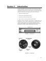
Section 1. Introduction
The heart of the OBS-3A monitor is an OBS“ sensor for measuring turbidity
and suspended solids concentrations by detecting near infrared (NIR) radiation
scattered from suspended particles. With a unique optical design, OBS sensors
perform better than most in situ turbidity sensors in the following ways:
1.
Small size and sample volume
2.
Linear response and wide dynamic range
3.
Insensitivity to bubbles and organic matter
4.
Rejects effects of ambient light and temperature change.
The OBS-3A includes a temperature sensor and may be equipped with pressure
and conductivity sensors. Batteries and electronics are contained in a housing
capable of operating at depths of up to 300 meters, depending on which
pressure sensor is installed. A survey cable may be used to tow the OBS-3A
and a depressor weight by clamping a cable harness to the housing.
362 mm (14.3”)
USE HOSE CLAMPS HERE
76 mm
(3.0”)
FIGURE 1-1. Dimensions
FIGURE 1-2. Components
1-1
Section 1. Introduction
Depending on the number of sensors and the statistics selected, the OBS-3A
can log as many as 200,000 lines of data (one per hour for 23 years) including:
time, date, depth, NTUs, oC, and salinity. When sampling with a full suite of
sensors, the unit will run about 300 hours. When using the instrument for
surveys, the data are captured by a PC running the OBS-3A Utility in the log
file created at initialization.
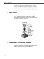
1.1 OBS Sensor
The OBS sensor consists of an infrared-emitting diode (IRED) with a peak
wavelength of 875 nm, four photodiodes, and a linear temperature transducer.
The IRED produces a conical beam with half-power points at 50o (FIGURE
1.1-1). The IR scattered between 140o and 160o is detected after passing
through a daylight-rejection filter and is proportional to turbidity and sediment
concentration. See Section 10—Specifications.
FIGURE 1.1-1. Anatomy of an OBS Sensor
1.2 Temperature and Optional Sensors
Temperature is measured with a fast-response, stainless steel-clad thermistor.
Pressure is measured with a semiconductor piezoresistive strain gage.
Conductivity is measured with a four-electrode conduction-type cell. Working
depths for available pressure sensors are listed in TABLE 2.1-1.
1-2
Section 2. Instrument Setup
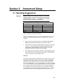
2.1 Mounting Suggestions
CAUTION
Maximum depth for the OBS-3A housing is 300 meters.
Working depths for individual instruments are limited by the
installed pressure sensor. If exceeded, the pressure
sensor will rupture and the housing will flood.
TABLE 2.1-1. Working and Maximum Depths
Pressure Sensor
0.2 Bar
1 Bar
5 Bar
10 Bar
20 Bar
Working Depth
0 - 2 meters
0 - 10 meters
0 - 50 meters
0 - 100 meters
0 - 200 meters
Maximum Depth
3 meters
15 meters
75 meters
150 meters
300 meters
(1 Bar = 10 dBar # 10 meters of fresh water)
Schemes for mounting the OBS-3A will vary with applications, however, the
same basic precautions should be followed to ensure the unit is not lost or
damaged.
x
The most important general precaution is to orient the unit so that the
OBS sensor “looks” into clear water without reflective surfaces.
x
Nearly all exposed parts of the instrument are made of Delrin, a strong but
soft plastic. Always pad the parts of the OBS-3A housing that will
contact metal or other hard objects with electrical tape or neoprene.
Expanded polyethylene tubes make excellent padding.
x
Never mount the instrument by the end-caps or attach anything to them.
This could stress the screws holding the unit together, cracking either the
end-caps or pressure housing, and cause a leak.
Moorings
The most convenient means for mounting the unit to a frame or wire is to use
large high-strength nylon cable ties (7.6 mm or 0.3" width) or stainless steel
hose clamps. Use at least six cable ties or two hose clamps for redundancy.
Position the clamps on the inner 2/3rds of the pressure tube, labeled “USE
HOSE CLAMPS HERE”, so stress is not transmitted to the ends (see FIGURE
1-1.). First cover the area(s) to be clamped with tape or 1/16" (2 mm) neoprene
sheet. Clamp the unit to the mounting frame or wire using the padded area.
Do not tighten the hose clamps more than necessary to produce a firm grip.
Over tightening may crack the pressure housing and cause a leak. Use spacer
blocks when necessary to prevent chafing the unit with the frame or wire.
2-1
Section 2. Instrument Setup
Surveys
The OBS-3A will usually be towed from a cable harness for surveys. The
serial cable supplied with the unit is strong enough to tow the OBS-3A and a
5-kg depressor weight however; the towing forces must be transmitted to the
pressure housing and not to the connector. To provide strain relief for the
connector, attach a cable grip about 30 cm above the SUBCONN® connector
(FIGURE 1-2) and attach a short length of 1/8" (3 mm) wire rope to the cable
grip. Clamp the wire rope to the pressure housing in the clamping area with
two stainless steel hose clamps. Provide a small loop of slack cable between
the cable grip and connector and put chafe protection on the sensor head where
it contacts the wire rope.
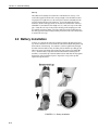
2.2 Battery Installation
If unit is wet, perform the following operations with the unit held sensor end
up. Remove the three hex screws from the end with the handle and pull the cap
down and out of the housing. Use caution if you have significantly changed
elevation since the OBS-3A may be under pressure and the cap could pop out.
Then wipe water from inside walls of the tube with a paper towel (FIGURE
2.2-1). Slide the battery clip back and insert the batteries with the positive
terminal (+) toward the clip. Push the batteries down and slide the clip against
the housing wall to hold them in place. Inspect the o-ring in the cap and
replace the cap and screws.
FIGURE 2.2-1. Battery Installation
2-2
Section 2. Instrument Setup
For extended deployment time, lithium batteries are a good alternative to
alkaline batteries. Campbell Scientific sells a D-cell-sized battery spacer
(pn 21906) that allows lithium D-cell batteries to be used with the OBS-3A.
Lithium D-cell batteries have a higher voltage than their alkaline counterparts,
necessitating the spacer. Campbell Scientific does not sell lithium D-cell
batteries.
2-3
Section 2. Instrument Setup
2-4
Section 3. Operations
3.1 Software Installation
Insert the CD and select “Install OBS-3A Utility”. Follow the installation
wizard to install the software. This utility is your interface with the OBS-3A.
As part of the installation, a system-maintenance program is included.
Communication drivers exist on the CD.
The main purpose of this section is to explain how to program and operate the
OBS-3A with the OBS-3A Utility. It covers: 1) turning the OBS-3A ON and
testing the sensors, 2) setting it up to sample in one of its four modes, 3)
recording data with a PC or uploading data from the OBS-3A, 4) importing
data into a spreadsheet, 5) plotting data with the OBS-3A Utility, and 6)
turning the OBS-3A OFF.
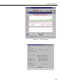
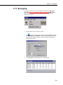
3.2 Running OBS-3A Utility
1.
Select the OBS-3A Utility program to start the utility and open the
Data window and toolbar.
2.
The OBS-3A Utility will create a new data log file and prompt you to
accept the name (see FIGURE 3.2-1). Files are automatically named
with Greenwich Date and Time as follows:
OBS3A_20010808_172433.log. Or you can designate your own file
name and destination by choosing No (see FIGURE 3.2-2).
FIGURE 3.2-1. New Data Log Prompt
FIGURE 3.2-2. Designating Your Own File Name and Destination
3-1
Section 3. Operations
Data received from OBS-3A while it is connected to the PC will be
stored in this file (see FIGURE 3.2-3).
FIGURE 3.2-3. Data Window (above) and OBS-3A Utility’s Toolbar
3.
Connect the OBS-3A to a PC with the test cable (FIGURE 3.2-4).
FIGURE 3.2-4. Connections and Wiring of Field Cable
3-2
Section 3. Operations
4.
Click
Connect/Disconnect to get a green light and synchronize
the OBS-3A clock with your PC by clicking
.
3.3 Pull-Down Menus
OBS-3A Utility has four pull-down menus for Files, OBS, View, and Help
(see FIGURE 3.3-1).
FIGURE 3.3-1. OBS-3A Utility Pull-Down Menus
The Files menu allows you to select the location and formatting for OBS files.
Files can be opened as plots or ASCII text that can be brought into spreadsheet
programs or text editors. Plot files are displayed graphically.
The View Menu controls the display on your PC. Switches are provided for:
x
Toolbar toggles the icons to ON or OFF.
x
Status bar toggles the Status Bar at the bottom of the screen to ON or
OFF.
x
Data Window pops the data window into view
The OBS menu allows you to put the instrument into a low power Sleep, or
have the instrument make a Barometric Correction.
3.4 Communication Settings
The
Plot and Port Settings button has a serial port tab that is used to
configure the PC communication settings. The default communication settings
are: 115 kbs, 8 data bits, no parity, no flow control. These settings will work
for most applications and with most PCs. In order to pick a slower baud rate
for an older PC or to avoid data-transfer errors, select the desired rate from the
dialog box and click Apply (see FIGURE 3.4-1). The rate adjustment takes
two seconds. If your PC is set to the wrong rate for some reason, use the check
3-3
Section 3. Operations
box to select ONLY change host computer port. Then click Apply and the
button.
If you get the OBS-3A information box, the baud rate of the unit is
synchronized with your PC. If you don’t get an information box, repeat the
above procedure.
FIGURE 3.4-1. Dialog Box for Changing Baud Rate
3.5 Testing Sensors
1.
Before daily operations and deployments, verify the instrument works by
clicking
Open Plot, and then clicking
installed sensors and click Start Survey.
2.
Survey. Select all
Wave your hand in front of the OBS sensor; the turbidity signal on the top
plot of FIGURE 3.5-1 will fluctuate and data will scroll.
3. Blow on the temperature sensor to observe an increase in temperature (red
trace on the middle plot of FIGURE 3.5-1).
3-4
4.
Blow into the pressure sensor and a small elevation in the pressure signal
will occur (bottom plot of FIGURE 3.5-1).
5.
Dip the sensor in salty water and conductivity will increase (blue trace on
middle plot).
6.
OBS-3A Settings to view time, serial numbers, depth
Click
corrections, and software versions (FIGURE 3.5-2).
Section 3. Operations
FIGURE 3.5-1. Test Data Sample
FIGURE 3.5-2. Window for Viewing Instrument Information
3-5
Section 3. Operations
3.6 Water-Density and Barometric Corrections
Since depths are estimated from pressure measurements, it is important to set
the water temperature and salinity so the OBS-3A can correct for water density
and calculate depth in meters or feet (this will not affect temperature or salinity
measurements). Also, the sensor measures absolute pressure so another
correction must be made for barometric pressure. Be sure to do this while the
OBS-3A is at the surface. Doing so when the instrument is submerged will
result in large errors in the depth measurement. The error will be
approximately equal to the instrument depth when the correction is made.
Depending on the magnitude of barometric pressure fluctuations at the
sampling site and the desired accuracy, you may want to correct data for
atmospheric effects using barometric pressure simultaneously recorded at a
nearby site.
3.7 Sample Statistics
Three types of statistics can be selected for the OBS-3A measurements.
1.
Measures of central tendency, the mean and median.
2.
Measures of variation or spread within a sample, the standard deviation (V)
and cumulative percentages, such as X25 and X75 (where X is the measured
depth or NTU)
3.
Wave statistics, significant height and dominant period.
Statistics are computed for each sample and logged in the FLASH. The raw
data are not saved. The mean is the arithmetic average of the values (¦ x / n),
where ¦ x is the sum of the sample values (x) and n is the number of values
(sample size). The median (X50) is the value that exceeds 50% of the sample
values and is the best measure of central tendency when a sample has outliers.
The percentages, X25, X50, X75, etc. exceed 25, 50, and 75% of the sample
values. The OBS-3A uses a spectral method developed by the U.S. Army
Corps of Engineers to calculate wave heights in depth units and periods (Hs and
Ts). Hs is the average height of the one-third largest waves, and reports it in the
selected depth units (meters or feet). Ts, is the time in seconds associated with
the peak spectral-density in the wave spectrum.
3.8 Definitions
The following definitions are useful when programming the OBS-3A.
Interval: The time in seconds between the start of one sample and the
beginning of the next. In cyclic mode, this is the time between samples, and in
setpoint mode, there are two intervals, one slow and the other fast. The
interval must be longer than the duration plus some time for statistical
computations. OFW will prompt you if too short an interval is selected.
Duration: This is the length of time in seconds that the OBS-3A is measuring
its sensors. The duration must always be less than the interval. The minimum
duration is five seconds and the maximum is the longer of the wave record
3-6
Section 3. Operations
length or the 2048 / rate. Note: the product of the rate and the duration cannot
exceed 2048.
Rate: Rate is the frequency of sampling for the duration of measurements. All
sensors are sampled at the same rate, typically 2, 5, 10, or 25 times per second
(Hz). For example, a rate of 25 Hz for a 60-second duration will produce a
sample with 1500 measurements for each sensor. When wave statistics are
chosen, the rate must be selected in the Wave Setup box.
Power: This indicates the percentage of time over the duration of a sample that
sensors are ON. Higher power levels mean larger samples, better statistics, and
shorter battery life. Lower levels spare the batteries but result in more random
noise in sample statistics.
Record Length: When wave measurements are selected, this sets the time in
seconds for which depth measurements are made for the wave-spectral
computations. Use a record length of 512 seconds for inshore waters (lakes
and rivers), protected bays and estuaries. For coastal waters with intermediate
periods (6 to 9 seconds) use 1024 seconds. For the open ocean select a record
length of 2048 seconds to record long period waves (Ts > 10 seconds).
Depth: This is the user’s best estimate of the water depth when the OBS-3A is
deployed. It is an initial value needed by the unit to compute wave heights and
correct for the attenuation of dynamic pressure with depth. When depth is
specified in the Wave Setup box, the OBS-3A automatically measures height
above bottom after reaching the deployment depth.
Height Above Bottom: This is distance above the bottom in meters or feet
where the OBS-3A will come to rest after it is deployed. It is an alternative
initial value used by the unit to correct for pressure attenuation. When height
above bottom is selected, depth is automatically computed once the unit has
come to rest.
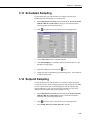
3.9 Sampling Schedules
The main factors that need to be considered when setting up OBS-3A sampling
schedules include:
x
Sampling interval needed to characterize the processes of interest (e.g.
water-level fluctuations, flood and transport duration, tidal and surf
conditions, etc.).
x
Maximum sediment concentration.
x
Statistical requirements, such as sample size and sampling rates.
x
Battery capacity.
The goal is to pick a sampling scheme that gets essential information without
taking too many samples or sampling too often. Inefficient sampling produces
a data avalanche, unnecessary processing, and excessive battery consumption.
Sampling schedules are set with the interval, duration, and rate parameters.
Interval sets the time in seconds between the start of one sample and the
beginning of the next, e.g. how often data are recorded. Select the longest
3-7
Section 3. Operations
interval that will show the changes in turbidity and water depth that you wish
to investigate. Rate sets the number measurements per second, in Hz, taken
during a sample. The quicker turbidity and depth change, the higher the
sampling rate should be to get a stable average value for a sample. Finally,
Duration sets the period of time for measurements and how long sensor
outputs will be averaged. For example, with an interval of 30 seconds and a
duration of five seconds, the OBS-3A will make measurements for five
seconds starting every 30 seconds. The number of measurements in a sample
(sample size) is the product of the duration and the rate. So if the rate was 25
Hz in the prior example, the sample size would be 5 X 25 = 125 measurements.
TABLE 3.9-1 provides some recommended ranges for these parameters in
various sampling environments. Always select duration and rate to give a
sample size of at least 30, and to reduce random sampling noise below 50% of
its maximum value, select them to give a size greater than 200.
TABLE 3.9-1. Sampling Schedules
Environment
Rate (Hz)
Duration (sec)
Interval
River/Stream
Beach
Estuary
2-5
5-25
5-10
30-100
30-200
10-60
300-900
60-900
600-3600
3.10 Sampling Modes
Survey: Select the survey mode when operating the unit with a cable
connection to a PC and when high data rates are desired. Data can be logged
with a PC at rates up to 120 lines per minute (2 Hz).
Cyclic sampling: Use cyclic sampling to record data internally in the 8
Mb, non-volatile FLASH memory at regular intervals, e.g. every 1, 5, 15, or 30
minutes. Depending on the number of sensors measured and the statistics
selected, the OBS-3A can log as many as 200,000 lines of data (one per hour
for 23 years) including: time, date, depth, NTUs, oC, and salinity.
Scheduled sampling: The OBS-3A can be scheduled to sample at
specific times in hours and minutes on a 24-hour clock using this mode.
Setpoint sampling: Use this mode for fast sampling of events such as
storms, floods, dredging operations, and construction activities. The unit will
revert to slow recording between events. Sample events two to five times
faster than the rate chosen for the periods between events. For example,
program the OBS-3A to sample slowly for a duration of 30 seconds every 900
seconds (15 minutes), and to sample at a fast rate every 180 seconds (three
minutes), when the turbidity level exceeds a specified setpoint.
3-8
Section 3. Operations
3.11 Surveying
If you have a pressure sensor, click the OBS menu and select Barometric
Correction (do not do this when the OBS-3A is submerged). The OBS-3A
takes about five seconds to measure the surface pressure and compute a
barometric correction.
1. Connect OBS-3A to PC with survey cable.
2.
Use
to select: sensors, lines per minute, depth units (Meters or Feet),
water Temperature, and Salinity. Selection of temperature and salinity
only affects the depth calculation. It does not influence temperature or
salinity measurements.
3. Click Start Survey and check data flow in data window.
3-9
Section 3. Operations
4. A file for logging data was created when you started the OBS-3A Utility.
Open and import the log file
You can review data at any time with
directly into an Excel spreadsheet for post-survey processing and plotting
(see Section 3.18—Excel Spreadsheets)
3.12 Cyclic Sampling
This mode is for logging data at regular time intervals such as 1, 10, 15, 30,
etc. minutes for example.
1.
Request Barometric Correction from the OBS menu. Be sure to do this
while the OBS-3A is at the surface. Doing so when the instrument is
submerged will result in large depth errors.
2.
and select sensors, statistics, depth units (meters or feet), water
Click
temperature, and salinity. Selection of temperature and salinity only
affects the depth calculation. It does not influence temperature or salinity
measurements.
3.
Configure the Wave Setup if you want to measure wave heights and
periods (see Section 3.8—Definitions). Do this before scheduling the
other sample parameters.
4. Select Interval, Duration, Rate, and Power level; see recommendations
in “Sampling Schedules” (Section 3.9). The duration must be longer than
the Record Length. The minimum duration for the Record Length will
be computed and displayed by the OBS-3A Utility.
5.
3-10
Click Start Sampling to begin logging data. Unplug test cable; install
dummy plug and locking sleeve. The instrument is ready for deployment.
Section 3. Operations
3.13 Scheduled Sampling
Use this mode when you want the OBS-3A to sample at specific times,
scheduled by hours and minutes, on a 24-hour clock.
1.
Request Barometric Correction from the OBS menu. Be sure to do this
while the OBS-3A is at the surface. Doing so when the instrument is
submerged will result in large depth errors.
2.
Click
3.
Use the Start Times block to schedule sampling.
4.
Click Start Sampling to record data. Monitor the data window to verify
that data are being logged.
5.
Switch the COM port off (red) with the
6.
Unplug test cable; install dummy plug and locking sleeve. The instrument
is ready for deployment.
and select items as described in Cyclic sampling section.
icon.
3.14 Setpoint Sampling
Use this mode when you want the OBS-3A to sample at a faster rate during
events such as storms, floods, dredging operations, and construction. The OBS3A will switch from the slow to fast sampling rate when the setpoints and
logical conditions you select are exceeded. It will return to the slower rate
when the selected setpoints and logical conditions are met.
1.
Request Barometric Correction from the OBS menu. Be sure to do this
while the OBS-3A is at the surface. Doing so when the instrument is
submerged will result in large depth errors.
2.
Click
3.
Select SLOW Interval and FAST Interval in seconds.
and select items as described in Cyclic sampling section.
3-11
Section 3. Operations
4.
Select setpoint values for transitions to fast sampling (SLOW>>>FAST)
and slow (FAST>>>SLOW) rates.
5.
Select one of the five logic criteria with the radio buttons.
6.
Click Start Sampling to record data. Monitor the data window to verify
that data are being logged.
7.
Switch the COM port off (red) with the
8.
Unplug test cable; install dummy plug and locking sleeve. The instrument
is ready for deployment.
icon
3.15 Data Retrieval
3-12
1.
Remove dummy plug and connect OBS-3A to PC with test cable.
2.
Run the OBS-3A Utility (see Section 3.2).
3.
Check the Data Window to verify the instrument is transmitting data.
4.
Click
a file.
5.
Highlight the data with the start and end times you want.
6.
Click Browse, select a destination file and click OK.
to end data collection and use
Offload Data to save data in
Section 3. Operations
7.
Wait for the progress bar to disappear and examine data as a plot or test
file (Section 3.17—Graphing and Printing).
3.16 Shutdown
From the OBS menu (see Section 3.11—Surveying), select Sleep. See menus
shown in the following section.
3.17 Graphing and Printing
1.
Use File menu to select how data file will be opened.
2.
and select a file to view.
Print will print a graph when
Click
data file is Open As Plot. To print a text file, Open As Text, and use the
Word Pad file print functions. For spreadsheet operations, see next section.
button is also used for communication
The Plot and Port Settings
settings (see Section 3.4—Communication Settings).
3.
Use the Min and Max and Sample Range (Start and End) values to
bracket the data you need on the graph. Plot Width allows the graph to be
sized to fit a PC screen. On the depth plot, select Max = 0 and Min = the
maximum depth to display depth increasing downward.
3-13
Section 3. Operations
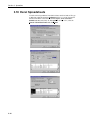
3.18 Excel Spreadsheets
To make an Excel spreadsheet from OBS-3A data, start Excel and set file type
to All. Open a data file and select Delimited in Step 1 of 3 of the Text Import
Wizard. Click Next > and select the delimiter Space; Treat consecutive
delimiters as one; and {none} for Text qualifier. In Step 3 of 3, select the
General Column data format and click Finish.
3-14
Section 3. Operations
3.19 Erasing Data Memory
To erase the flash data memory, do the following:
1) Click on the
Terminal Mode Icon.
2) At the OBS> prompt, type ‘sl 543210’ to unlock the system.
3) Type ‘ef 33’ plus Enter, then ‘ef 55’ plus Enter.
4) The erased-block-interval counter will be displayed every 100 blocks.
There are 8192 blocks and the process takes ~ 1/2 hour.
5) When done, type ‘fw’ to reset the file pointer.
By following this procedure data in the FLASH memory is erased, so be
careful!
3-15
Section 3. Operations
3-16
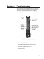
Section 4. Troubleshooting
This section will help you isolate problems that can be easily fixed such as
cable-continuity, processor reset, and battery replacement from serious ones
such as sensor, computer and electronic malfunctions, and damaged
mechanical parts that will require our help. The problem symptoms are shown
with underlined, bold text.
FIGURE 3.19-1. Component locations
Unit does not communicate with PC.
There are several possible causes for this symptom.
1.
The test/umbilical cable is damaged or improperly connected.
2.
The OBS-3A is sleeping and will not wake up.
3.
The batteries are dead.
4-1
Section 4. Troubleshooting
4.
The OBS-3A and PC are not set to the same baud rate or communication
protocol (e.g. RS-232, USB, RS-485).
x
and check port settings on the serial port tab. The default
Click
baud rate is 115.2 kb. If the PC is not set to this speed, follow the
steps in Section 3.4 to set it.
x
If the OBS-3A still fails to respond, try changing PC speeds and
until communication is established (e.g. 57.6, 38.4, 19.6,
clicking
9.6 kb, etc.). If this fails, switch the PC back to 115.2 kb and go to the
next step.
x
Reconnect the cable and try
x
Replace the main batteries; see Section 2.2 and try
x
If you have a survey cable, connect instrument to external power and
try
x
.
.
.
Remove the unit from the pressure housing and press and release the
RESET button. Try
.
Power failed due to battery clip corrosion or a broken power wire.
Check for a broken red wire connecting the battery tube and circuit board.
Green powder or tarnish on the battery contact parts indicates salt-water
corrosion. Remove the electronics from the pressure housing. Pull batteryclip-retainer pin out with needle-nose pliers and slide the clip from its track.
Clean the corroded surfaces of clip and track with a Scotch-brite® pad and
reassemble unit.
OBS or other sensor malfunction.
4-2
x
Inspect for physical damage such as a broken or bent thermistor, a dirty
conductivity sensor, or an OBS sensor fouled with marine growth.
x
Open unit and inspect for broken sensor and communication wires and
loose connectors (FIGURE 3.19-1).
x
Check sensor power by starting Survey mode
and selecting all
sensors. Green LEDs should illuminate for installed sensor.
x
If the depth sensor reads high and does not change, it may need to be
cleaned (see pressure-sensor maintenance, Section 5.2).
x
If the sensors appear to be in working order, the digitizer or
microcontroller may be damaged. Such problems usually require factory
service.
Section 4. Troubleshooting
Bright sun near the surface ( < 2 meters) or black-colored sediments cause
erroneous OBS readings.
Do not survey in shallow water between 10:00 and 14:00 local time and avoid
areas with suspended black mud.
Changing the water temperature in the setup dialog box does not change
the temperature measurement.
This is normal. Temperature inputs only change the water density correction
used to convert pressure to depth.
OBS-3A indicates different NTU values in the field than other
turbidimeters.
Not all turbidity meters read the same! OBS sensors are checked with a Hach
2100N laboratory instrument, using U.S. EPA-approved, formazin turbidity
standards before leaving our factory. Turbidimeters other than the 2100N will
read different NTU values on natural water samples.
OBS-3A indicates different suspended sediment levels in the field than in
the laboratory.
This results from a change in sediment size or color (see Section 8). You may
have to perform a field calibration with water samples.
4-3
Section 4. Troubleshooting
4-4
Section 5. Maintenance
5.1 OBS Sensor
The OBS sensor must be kept clean to measure sediment concentration or
turbidity accurately. A gradual decline in sensitivity over a period of time
indicates fouling with mud, oil, or biological material. Regular cleaning with a
water jet, mild detergent and warm water, or a Scotch-bite abrasive pad will
remove most contaminants encountered in the field. Solvent or mineral spirits
on cloth can be used to remove oil or grease however, do not use MEK,
benzene, toluene, or electronic cleaners as they could damage the OBS
window. At the conclusion of each survey or deployment, clean the OBS. If
thick bio-fouling has developed:
1.
Scrape the material off the window with a flexible knife, taking care not to
scratch it.
2.
Tape a strip of 400 to 600-grit wet/dry sandpaper on the edge of a bench
top.
3.
Add a few drops of water and rub the sensor window on the wet
sandpaper, using the counter edge for a guide.
4.
Continue until the sensor is smooth and pit-free.
Polishing with abrasives can be done as needed until approximately 1 mm of
epoxy has been removed. Deeper polishing may damage the IR source.
Check the calibration of the sensor with formazin after cleaning with abrasives;
see Section 6—Calibration.
5.2 Pressure Sensor
The strain gage sensor is located under a perforated disk and spring-clip
(FIGURE 1-2) that protects the Hastelloy diaphragm isolating it from water.
Do not touch the diaphragm with tools or pointed objects, as the instrument
will leak if it is pierced. Clean the sensor with a water jet directed at the disk
after each survey or deployment to flush sediment from between the disk and
the sensor. Do not allow sediment to dry on the sensor diaphragm, as it is
difficult to clean and will influence accuracy. If this occurs, remove the spring
clip and disk with plastic tweezers then gently wipe sediment off the
diaphragm with a cotton-tipped swab. Replace the disk and spring clip then
flush with a water jet.
5.3 Conductivity Sensor
The conductivity sensor is very fragile and is enclosed in a hole behind the
OBS sensor. Do not poke it with any tool or object as the electrodes may be
damaged. Routine cleaning should only be done with a water jet directed
alternately from the side and top of the sensor well. This should be done daily
5-1
Section 5. Maintenance
during surveys or after each deployment. A sensor that has been stored dry
should be soaked in water for 15 minutes prior to use.
If the sensor becomes fouled with sediment, oil, or biological material,
conductivity will decline over a period of time indicating cleaning is necessary.
If a water jet fails to remove contaminants, the sensor can be flushed with hot
soapy water or warm alcohol. Do not use solvents. The last step in the
cleaning process should always be to flush with clean water.
5.4 Batteries
The unit runs on three D-size alkaline batteries. Buy the expensive ones with
the most distant pull date (“use before May 2012”). With all sensors installed,
the OBS-3A will run 400 hours in survey mode and for as long as 8000 hours
in one of the logging modes.
CAUTION
Always put OBS-3A to sleep when it will not be used for a
while to conserve battery capacity (see Section 3.16—
Shutdown).
Refer to FIGURE 2.2-1 for installing batteries. Put the unit on a padded
surface and remove the three screws from the end with the handlebar using the
5/64" hex wrench provided in the spares kit. Grasp the handlebar, turn the
sensor end up and pull the cap straight out of the pressure-housing tube.
Immediately wipe up any water from inside the tube. Stand the unit up on the
sensor end and remove the desiccant bags. Slide the clip away from the
batteries until the spent cells pop up and can be slid out of the tube. Insert
fresh batteries in the tube with the positive terminal (+) up. Press them down
and slide the clip over the batteries until it contacts the tube wall. Replenish
the desiccant bags and clean and regrease the O-ring. Replace the end cap. Do
not over tighten the screws.
Battery life will depend on the percentage of time the unit is sampling.
TABLE 5.4-1 shows battery life as a function of sample duration and interval
to assist with planning your setup. Pick a power-efficient sampling schedule
that meets your scientific objectives.
TABLE 5.4-1. Battery Life (Hours)
Interval
(Sec.)
60
600
900
1800
3600
101
100%
1300
> 8000
> 8000
> 8000
> 8000
602
50%
NO
5450
> 8000
> 8000
> 8000
Duration in seconds (% Power)
601
1202
1201
2563
100%
50%
100%
10%
NO
NO
NO
NO
2080
3150
1100
1460
2970
5450
1600
2110
5160
> 8000
2950
3815
> 8000
> 8000
5150
6400
2561
100%
NO
530
785
1510
2810
10243
10%
NO
NO
NO
1120
2110
NO = Not possible; 1 = All sensors; 2 = OBS & depth sensors; 3 = Wave calculations.
5.5 Pressure Housing
The pressure housing and O-ring seals require little maintenance unless the
housing has been opened since the last service. However, it should be
5-2
Section 5. Maintenance
carefully inspected every six months and serviced before all deployments
longer than one month.
1.
Disassemble O-ring seals and inspect mating surfaces for pits and
scratches.
2.
Inspect O-rings for cuts and nicks; replace if necessary using spares
provided.
3.
Clean O-rings and mating surfaces with a cotton swab and alcohol.
Remove fibers from groove and mating surfaces then grease O-rings with
DOW Compound 55 and reassemble.
5.6 Antifoulant Coatings
Clear TBTA antifoulant coating or toxin-impregnated collars can be used for
monitoring in biologically active waters. TBTA prevents most marine algae
and encrusting animals from growing on optical surfaces for up to two months
with minimal loss of IR transmission. It is illegal to use TBTA in many places
so check applicable water quality regulations in your area before using TBTA
coated OBS sensors. Use of TBTA is the sole responsibility of the user.
5.7 User-serviceable Parts
See Section 10—Specifications for a list of user-serviceable parts.
5-3
Section 5. Maintenance
5-4
Section 6. Calibration
6.1 Turbidity
This section briefly describes the materials and equipment you will need and
the basic procedures for calibrating OBS sensors with AMCO Clear and
sediment. All sensors are factory calibrated with AMCO Clear and include a
calibration certificate expressed in nephelometric turbidity units (NTU).
AMCO Clear is available from GFS Chemicals Inc. (800-858-9682;
www.gfschemicals.com). It is approximately three times more expensive than
formazin per NTU-liter, however: 1) it is guaranteed to be stable for one year
and has <1% initial lot-to-lot accuracy; 2) AMCO particles are small and
uniform in size and shape (0.31 ±0.1m versus 1.3 ±0.6m for formazin); and
3) it does not flocculate or settle so stirring is not required. AMCO Clear must
be made specifically for the OBS sensor.
Formazin can be purchased from the Hach Company (800-227-4224;
www.hach.com)); request the certificate of analysis when ordering it. Hach
also supplies premixed, StablCal which is like formazin except that it can be
stored for two years while maintaining ±5% of its nominal NTU value.
We strongly advise that the same turbidity standard be used throughout a study
(e.g. do not switch between AMCO and formazin standards). Also, AMCO is
premixed by the manufacturer and must be used in the container it was shipped
in.
Turbidity calibration is organized into steps for Preparation; recording values
with OBS-3A Utility; and Production of Standards. After completing the
preparations and starting OBS-3A Utility, you must alternate between the
OBS-3A Utility and standard-production procedures.
6.1.1 Equipment and Materials
x
4000 NTU AMCO Clear, StablCal, or formazin
x
4” and 6” diameter black polyethylene containers. Concrete sample
containers (Cat. # TC-4, Deslauriers Inc., 800-743-4106;
www.deslinc.com) work well for this.
x
2-liter, Class A volumetric flask
x
100 ml TD volumetric pipette
x
25 ml TD measuring pipette
x
2 gallons filtered distilled water (purified water from the super market
works fine)
x
Slotted stainless steel stirring spoon
6-1
Section 6. Calibration
6.1.2 Preparation
1.
Experience has shown that only three calibration points are needed to get
sub-1% accuracy. It is recommended to do one for clean filtered water, a
midrange value (e.g. 125, 250, 500 or 1000 NTU) and one at the high end
of the desired measurement range (e.g. 250, 500, 1000, or 2000 NTU).
2.
Scrub the sensor, container, spoon, and glassware with detergent and water
and rinse everything twice with filtered water.
3.
To avoid interference from incandescent and solar IR, perform calibrations
under fluorescent lighting and make field checks in the shade.
4. Start the OBS-3A Utility Software and wake the OBS-3A.
6.1.3 OBS-3A Utility Software Steps
1.
WARNING
6-2
Open the calibration dialog box with
and click the NTU button.
Follow the instructions to place the OBS-3A in a turbidity standard.
You cannot change the OBS-3A calibration after
exiting the calibration dialog box.
2.
Enter the standard value in the Value box of the calibration dialog and
click the Record button. If mg/l or ppm are selected, choose a sample
duration from TABLE 6.2-1.
3.
After the sample has been logged, the table and plot of calibration data
will be updated. Verify that the calibration value is what you intended it to
be.
4.
Prepare the next NTU standard and put the OBS-3A in it. Repeat steps 1
and 2 for all calibration values.
5.
After the calibration is complete, click the Compute button and inspect
the plot to verify that it resembles the example shown above.
Section 6. Calibration
WARNING
There is no way to cancel a calibration after the
Compute button is clicked.
Review the quality assurance checks discussed later in this section. Look at the
plot of residuals, which show the differences between the standard and
computed NTU values. The average residual magnitude should be less than
1% of the calibration range. For example, a calibration range of 2000 NTU
(maximum minus minimum NTU values) should produce an average residual
less than 20 NTU. Residuals higher than 1% of the calibration range indicate
that errors were made in the procedure. By inspecting the plot of residuals, you
can decide which values to repeat, edit, or delete. Repeat values using the
procedures described above. To edit a value,
6.
Click the Edit button; select the number of the calibration value you want
to change from the data table; enter the revised calibration value; and click
OK.
7.
The data table and plot will be updated. Use the Delete button to remove a
calibration value by number from the data table.
8.
Once satisfied with the calibration, click the Compute button and make a
final quality check.
9.
Use the Done / Exit button to return to the OBS-3A Utility.
6.1.4 Making Turbidity Standards
1.
For the zero NTU calibration point you will need a black 20”X14”X16”
container filled with clean tap water. A Rubbermaid plastic storage box
makes a suitable container.
2.
For calibrations from 50-250 NTU use a 6” diameter container with 2
liters of filtered water or a premixed standard. Hold the sensor in the
container so that the beam looks down and across the diameter to prevent
the beam from reflecting off the wall.
3.
A 4” diameter container can be used for solutions of 250 NTUs. Add one
liter of filtered water and the necessary amount of formazin. See TABLE
6.1-1 or the formula below for the preparation of standards.
4.
Stir the formazin solution with the spoon and position the OBS-3A in the
standard.
5.
Go to Step 2 of OBS-3A Utility Steps (Section 6.1.3).
The formula for preparing turbidity standards other than shown in TABLE
6.1-1 is:
Tstd
ª Vstk º
Tstk «
¬Vdw Vstk »¼
or
Vstk
ª Tstd u Vdw º
«¬ Tstk Tstd »¼
6-3
Section 6. Calibration
Where:
Tstd = Turbidity of the standard solution;
Tstk = Turbidity of the stock solution, usually 4000 NTU;
Vstk = Cumulative volume of stock solution at each calibration point;
Vdw = Initial volume.
TABLE 6.1-1. Mixing Volumes for Formazin
Standards
Formazin Volume
Vstk (ml)
Solution Turbidity
Tstd (NTU)
12.7
50
32.3
125
66.7
250
143
500
333
1000
1000
2000
6.2 Sediment
The procedure for sediment calibration is more involved than for turbidity. For
a modest charge we will pre-calibrate OBS sensors with sediment provided by
users. Call us for a quotation to perform this service.
CAUTION
The most common cause of errors in OBS data is improper
calibration.
Before proceeding with a sediment calibration, review Section 8 to learn about
factors that can influence the quality of your results. The most difficult part of
the procedure is maintaining a stable sediment concentration while the OBS
logs calibration values. This is straightforward when the material is dry,
completely disaggregated mud with particles smaller than ~20m. It becomes
more difficult the larger the sediment gets and special calibration equipment
may become necessary (see Section 9—References).
6.2.1 Equipment and Materials
6-4
x
Dry, completely disaggregated bottom sediment or suspended matter from
the monitoring site,
x
1-gallon (4 l) brown Nalgene polypropylene bottle with top cut off,
x
1-liter, Class A volumetric flask,
Section 6. Calibration
x
2 gallons filtered distilled water (purified water from the super market
works fine),
x
Hand-drill motor,
x
Paint stirrer.
6.2.2 Sediment Preparation
Sediment preparation is a critical factor in calibration quality. It is most
convenient to use dry material because it can be accurately weighed with an
electronic balance. However, this only works well for clean sand because
disaggregation produces a sediment size different than existed in the field. For
example, deep harbors with weak currents often have cohesive (sticky) mud
with high organic-rich flocculation. Disaggregation of the flocs will reduce the
particle size and change the OBS response. Sediment or suspended solids
concentration is the dry weight of sediment divided by the weight of the
sample (expressed in ppm) or by the volume of sample in liters (expressed as
mg/l). Usually the disaggregated particles will be finer than untreated
sediment. When dried sediment is used, verify that field estimates are accurate
by comparing the OBS results with direct samples of suspended matter. (See
Section 9—References: USGS Book 9.)
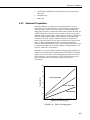
FIGURE 6.2-1 shows how different methods of disaggregating sediment can
change the relationship between turbidity and the concentration of suspended
material. This occurs because vigorous disaggregation produces more small
particles than less vigorous methods as well as more OBS signal per unit of
mass concentration. The result is higher signal levels for a given
concentration.
60
50
Turbidity (NTU)
40
3-min. Sonic Probe
30
15-min. Sonic Bath
20
Hand Shaking
10
0
10
20
30
40
50
Sediment Concentration (mg/l)
FIGURE 6.2-1. Effects of Disaggregation
6-5
Section 6. Calibration
Preparation
1.
Clean containers and glassware with detergent and rinse with filtered
water.
2.
Perform the calibration under fluorescent lighting.
3.
Based on the material, select the appropriate sample duration from TABLE
6.2-1.
4.
Open the calibration box with
values.
5.
After each addition of sediment compute mg/l or ppm with the equations
given below.
6.
Start the OBS-3A Utility and wake the OBS-3A. Click the mg/l or ppm
button.
and enter sediment concentration
TABLE 6.2-1. Sample Durations for
Sediment Calibrations
Sediment
Seconds
Clay
10
Silt
20
Fine Sand
40
Sediment concentrations are calculated with the following equations:
Ms
ª Ms º
Vi « »
¬ s ¼
mg/l
;
Ms
Mi Ms
ppm
Where:
Ms = Mass (mg) of sediment in suspension
Mi = Initial water mass, 1u Vi ( kg )
Vi = Initial volume (L)
U s = Sediment density (usually 2.65 u 10 3 mg / l )
6-6
7.
For the zero calibration point you will need a clean black 20” x 14” x 16”
container filled with clean tap water. A Rubbermaid plastic storage box is
suitable.
8.
Add 2 l of filtered water to the 1 gallon container submerging the sensor at
least 5 cm; tap bubbles off container walls.
Section 6. Calibration
9.
Weigh 5 to l0 equal increments of the sediment so that the total dry weight
will produce the maximum concentration expected at the monitoring site.
10. For each sediment standard, repeat Steps 2 through 4 of Section 6.1.3.
11. After all sediment values have been logged, follow Steps 6 through 9 of
Section 6.1.3 to complete the calibration.
6.3 Salinity, Pressure and Temperature
Calibrations
Due to the specialized equipment involved for salinity, pressure and
temperature calibration, it is recommended that the instrument be returned to
Campbell Scientific, Inc. if any of these sensors are not operating with
specified accuracy.
6-7
Section 6. Calibration
6-8
Section 7. Optics and Turbidity
Measurements
Turbidity is the cloudy appearance of a liquid produced by light scattered from
suspended matter. It is an apparent optical property that depends on the size,
color, and shape of scattering particles, and the instrument used to measure it.
In accordance with standard method 2130B and ISO 7027, turbidity is usually
measured with a 90o-scatterance nephelometer and reported in nephelometric
turbidity units (NTUs). Turbidity standards are discussed in Section 6.
FIGURE 6.3-1. Optical Particle Detectors
Light transmission in water is attenuated by scattering (deflection by water
molecules, and suspended matter) and absorption, which converts light to heat.
Attenuation, absorption, and scattering are inherent properties of water that are
affected only by impurities such as color and suspended organic matter.
Optically pure water is not readily available; however deionized water that has
passed through a 0.2 μm filter is adequate for most practical purposes.
There are dozens of turbidimeter designs, however most are configured in one
of the ways shown in FIGURE 6.3-1. These include: forward-scatterance, 90o
scatterance, and backscatterance nephelometers. Some instruments combine
two or more of these configurations and blend signals to produce a useful
output. The transmissometer measures attenuation, an inherent optical
property but is not approved for turbidity measurements except by ISO 7027.
OBS sensors have superior linearity in turbid water but a transmissometer is
more sensitive at low concentrations (<~25 mg/l). Data from turbidimeters
made by different companies should be compared cautiously. Inconsistencies
between instruments results from variations in light sources, detectors, optical
configurations and turbidity standards.
7-1
Section 7. Optics and Turbidity Measurements
Can turbidity be converted to suspended solids concentrations and viseversa?
In most situations, conversions between turbidity and suspended solids
concentrations will give misleading results because the conversion equates to
an apparent optical property, in relative units, with one precisely defined in
terms of mass and volume; these are "apples and oranges".
Conversion of turbidity to suspended solids concentration is recommended
only when:
x
Measurements are made with the same turbidimeter.
x
The turbidimeter is intercalibrated with a turbidity standard and suspended
matter from the waters to be monitored.
x
Particle size and composition do not change over the monitoring period.
Compliance with the last condition is crucial but virtually impossible to verify
in the field because it is difficult to sample particles in their natural state and
preserve them for laboratory analysis in a consistent and meaningful way.
7-2
Section 8. Factors Affecting OBS
Response
This section summarizes some of the important factors that affect OBS-3A
measurements and shows how ignoring them can lead to erroneous data. If you
are certain that the characteristics of suspended matter will not change during
your survey and that your OBS was factory calibrated with sediment from your
survey site, you only need to skim this section to confirm that no problems
have been over looked.
8.1 Particle Size
The size of suspended sediment particles typically ranges from about 0.2 to
500μm in surface water (streams, estuaries and the ocean). Everything else
being equal (size, shape, and color), particle area normal to a light beam will
determine the intensity of light scattered by a volume of suspended matter.
Results from laboratory experiments and natural material support this and
indicate a wide range of backscatter associated with very fine mud and coarse
sand (about two orders of magnitude). Laboratory tests with coarse silt to
medium sand material show that sensitivity changes by a factor of about 3.5
(see FIGURE 8.2-1). The significance is that size variations between the field
and laboratory and within in a survey area cannot be ignored.
10000
Silt
OBS Signal (mV)
Clay
Sand
1000
100
10
100
1000
10000
100000
Sediment Concentration (mg/l)
FIGURE 8.1-1. Response to Sand, Silt and Clay
8-1
Section 8. Factors Affecting OBS Response
8.2 Suspensions with Mud and Sand
As mentioned earlier, backscattering from particles is inversely related to
particle size on a mass concentration basis (see FIGURE 8.2-1). This can lead
to serious difficulties in flow regimes where particle size varies with time. For
example, when sandy mud goes through a cycle of suspension and deposition
during a storm, the ratio of sand to mud in suspension will change. An OBS
sensor calibrated for a fixed ratio of sand to mud will therefore indicate the
correct concentration only part of the time. There are no simple remedies for
this problem. The obvious thing to do is to take a lot of water samples and
analyze them in the laboratory. This is not always practical during storms
when the errors are likely to be largest. Do not rely solely on OBS sensors to
monitor suspended sediments when particle size or composition are expected to
change with time at a monitoring site.
1.0
Gain (V/g/l)
0.8
Gain = 8.3(D)
-0.6
0.6
0.4
0.2
0
50
100
150
200
250
Grain Diameter (microns)
FIGURE 8.2-1. Effects of Particle Size
8.3 High Sediment Concentrations
At high sediment concentrations, particularly in suspensions of high clay and
silt, the infrared radiation from the emitter can be so strongly attenuated along
the path connecting the emitter, the particle, and the detector, that backscatter
decreases with increasing sediment concentration. For mud, this occurs at
concentrations greater than about 5,000 mg/l. FIGURE 8.3-1 shows a
calibration in which sediment concentrations exceed 6 g/l cause the output
signal to decrease. It is recommended not to exceed the specified turbidity or
suspended sediment ranges unless calibrations extend over range “A” on
FIGURE 8.3-1.
8-2
Section 8. Factors Affecting OBS Response
5
A
Signal (V)
4
3
2
1
0
0
5
10
15
Sediment Concentration (g/l)
FIGURE 8.3-1. Response at High Sediment Concentrations
8.4 Sediment Color
Sediment color, after particle size, has a major effect on OBS sensitivity, and if
it changes, it can degrade the accuracy of measurements. Although OBS
sensors are “color blind”, “whiteness”, color, and IR reflectivity (measured by
an OBS sensor) are well correlated. Calcite, which is highly reflective and
white in color, will produce a much stronger OBS signal on a massconcentration basis than magnetite, which is black and IR absorbing.
Sensitivity to colored silt particles varies from a low of about one for dark
sediment to a high of about ten for light gray sediment; see FIGURE 8.4-1. In
areas where sediment color is changing with time, a single calibration curve
may not work. Resulting errors will depend on the relative concentrations of
colored sediments.
8-3
Section 8. Factors Affecting OBS Response
1.0
Calcite
Infrared Reflectance
0.8
Bytownite
0.6
Actinolite
0.4
0.2
Magnetite
0.0
0
2
4
6
8
10
Munsell Value (Black = 0)
FIGURE 8.4-1. IR Reflectance of Minerals
8.5 Water Color
Several OBS users have been concerned that color from dissolved substances
in water samples (not colored particles discussed in the previous section)
produces erroneously low turbidity measurements. Although organic and
inorganic IR-absorbing dissolved matter has visible color, its effect on OBS
measurements is small unless the colored compounds are strongly absorbing at
the OBS wavelength (875 nm) and are present in very high concentrations.
Only effluents from mine-tailings appear to produce enough color to absorb
measurable IR. In river, estuary, and ocean environments concentrations of
colored materials are too low by at least a factor of ten to produce significant
errors.
8.6 Bubbles
Although bubbles efficiently scatter IR, monitoring in most natural
environments shows that OBS signals are not strongly affected by bubbles.
Bubbles and quartz particles backscatter nearly the same amount of light to
within a factor of approximately four, but most of the time bubble
concentrations are at least two orders of magnitude less than sand
concentrations in most environments. This means that sand will produce much
more backscatter than bubbles in most situations and bubble interference will
not be significant.
The scattering intensity of mineral particles, bubbles, and suspended organic
material are shown in FIGURE 8.6-1. OBS sensors detect IR backscattered
between 140o and 160o, and where the scattering intensities are nearly constant
with the scattering angle. Particle concentration has the most important effect
8-4
Section 8. Factors Affecting OBS Response
in this region. OBS sensors are also more sensitive to mineral particles than
either bubbles or particulate organic matter by factors of four to six. In most
environments, interference from these materials can therefore be ignored. One
notable exception is where biological productivity is high and sediment
production from rivers and resuspension is low. In such an environment, OBS
signals can come predominately from plankton. Prop wash from ships and
small, clear mountain streams where aeration produces high bubble
concentrations are another probable source of erroneous turbidity readings.
10.000
T
o
Backscatter (90 - 180 )
Scattering Intensity
1.000
Bubbles
0.100
OBS
Minerals
0.010
Organic Material
0.001
0
20
40
60
80
100
120
140
160
180
Scattering Angle (T)
FIGURE 8.6-1. Scattering Intensity vs. Angle
8.7 Biological and Chemical Fouling
Sensor cleaning is essential during extended deployments. In salt water,
barnacle growth on an OBS sensor can obscure the IR emitter and/or detectors
and produce an apparent decline in turbidity. Algal growth in marine and fresh
waters has caused spurious scatter and apparent increases of OBS output. The
reverse has also been noted in fresh water where the signal increases after
cleaning the sensor window.
Prolonged operation in freshwater with high tannin levels can cause a varnishlike coatings to develop on an OBS sensor that obscure the IR emitter and
caused an apparent decline in turbidity. Cleaning algal and tannin
accumulation off OBS sensors is required more often during the summer
because warm water and bright sunlight increase biological and chemical
activity. See Antifoulant Coatings for alternatives to cleaning.
8-5
Section 8. Factors Affecting OBS Response
8-6
Section 9. References
See www.campbellsci.com/obs for a complete list of references.
Conner, C.S. and A.M. De Visser. 1992. A Laboratory Investigation of Particle
Size Effects on an Optical Backscatterance Sensor. Marine Geology, 108,
pp.151-159.
Downing, John and W.E. Asher. 1997. The Effects of Colored Water and
Bubbles on the Sensitivity of OBS Sensors. American Geophysical Union, Fall
Meeting, San Francisco, CA.
Downing, John and Reginald A. Beach. 1989, Laboratory Apparatus for
Calibrating Optical Suspended Solids Sensors. Marine Geology, 86, pp. 243249.
Gippel, C.J. 1995. Potential of Turbidity Monitoring for Measuring the
Transport of Suspended Solids in Streams. Hydrologic Processes, Vol.9, pp.
83-97.
International Standard ISO 7027. Second Edition 1990-04-15. Water Quality –
Determination of Turbidity. International Organization for Standardization.
Genève, Switzerland. 6 pages.
Lewis, Jack. 1996. Turbidity - Controlled Suspended Sediment Sampling for
Runoff-Event Load Estimation. Water Resources Research, Volume 32, No.
7, pp. 2299-2310.
Ludwig, K.A. and D.M. Hanes. 1990. A Laboratory Evaluation of Optical
Backscatterance Suspended Solids Sensors Exposed to Sand-Mud Mixtures.
Marine Geology, 94, pp.173-179.
Papacosta, K., J.A. Spair and M. Katz. The Rationale for the Establishment of
a Certified Reference Standard for Nephelometric Instruments. Advanced
Polymer Systems, Inc. Redwood City, CA.
Sadar, M. 1995. Turbidity Standards. Technical Information Series-Booklet
No. 12. Hach Company. Loveland, Colorado. 18 pages.
Standard Methods for the Examination of Water and Wastewater, 20th Edition.
1998. 2130 Turbidity. American Public Health Association et al. Washington,
DC.
Standard Methods for the Examination of Water and Wastewater, 20th Edition.
1998. 2540 B Total Solids Dried at 103-105°C. American Public Health
Association et al. Washington, DC.
Sutherland T.F., P.M. Lane, C.L. Amos, and John Downing. 2000. The
Calibration of Optical Backscatter Sensors for Suspended Sediment of
Varying Darkness Level. Marine Geology, 162, pp. 587-597.
U.S. Department of Agriculture. 1994. National Handbook of Water Quality
Monitoring, Part 600, USDA SCS, Washington, DC.
9-1
Section 9. References
U.S. Geological Survey. 2003. National Field Manual of the Collection of
Water-Quality Data. Book 9, Handbooks for Water-Resources Investigations.
Zaneveld, J.R.V., R.W. Spinrad, and R. Bartz. 1979. Optical Properties of
Turbidity Standards. SPIE Volume 208 Ocean Optics VI. Bellingham,
Washington. pp. 159-158.
9-2
Section 10. Specifications
MEASUREMENT RANGE
Turbidity (AMCO Clear) ............................... 0.4 to 4,000 NTU1
Mud (D50=20μm) .......................................... 0.4 to 5,000 mg/l
Sand (D50=250μm) ........................................ 2 to 100,000 mg/l
Pressure2 ........................................................ 0 to 10, 20, 50, 100, or 200 m
Temperature................................................... 0o to 35oC
Conductivity (salinity) ................................... 0 to 65 mS/cm (40 PSU, o/oo)
ACCURACY
Turbidity (AMCO Clear, 0-2,000 NTU)........ <2.0%
Mud (0.4-4,000 mg/l) ................................... 2.0% of reading
Sand (0.4-60,000 mg/l) ................................. 3.5% of reading
Pressure.......................................................... ±0.5% full scale
Temperature................................................... ±0.5oC
Conductivity .................................................. 1%
OBS SENSOR
Frequency ...................................................... 5 Hz
Drift over time ............................................... <2% per year
Drift over temperature ................................... 0.05% per oC
OTHER DATA
Maximum size sample .................................. 2048
Sampling rate ................................................. 1 to 25 Hz
Maximum data rate ........................................ 25 Hz
Data capacity ................................................. 8 Mbytes
Maximum number of data lines ..................... 200,000
Battery capacity ............................................. 18 Ahr
Maximum battery life ................................... 8,000 hours
Data protocols................................................ RS-232 / RS-485
Maximum housing depth .............................. 300 m (984 ft)
Infrared wavelength ....................................... 850 nm
Operating temperature range ......................... 0o to 35oC
Storage temperature range ............................. -20o to 70oC
PHYSICAL
Length / diameter .......................................... 362 mm (14.3”) / 76 mm (3.0")
Weight (w/o batteries) ................................... 1.5 kg (3.4 lbs)
Weight (submerged) ..................................... 0.2 kg (0.5 lbs)
Connector....................................................... MCBH-8-FS, wet-pluggable
SHIPS WITH
CSI # 21229 Accessory Kit
Resource CD
CSI # 20919 Software Support CD
REPLACEMENT PARTS
Alkaline D cells and the components of the 21229 Accessory Kit can be
purchased as replacement parts. Campbell Scientific model numbers and
product descriptions follow:
CSI # 20990 End Cap O-ring
CSI # 21145 Pressure Sensor Spring Clip
10-1
Section 10. Specifications
CSI # 21135 End Cap Screws, 8-32 x 3/8”, socket (5/64”)
CSI # 21120 Dummy Plug
CSI # 21122 Plug Locking Sleeve, Subconn® MCDLSF
CSI # 425 Alkaline D-Cells Batteries
CSI # 21136 Screws, #4-40 x 1/4”, socket
CSI # 20792 OBS-3A Test Cable, 2 m (6.5 ft)
CSI # 21149 Hex Driver, 5/64”
10-2
1
0-100, 0-250, 0-500, 0-1000, 0-2000, and 0-4000 NTU ranges are
available.
2
Range depends on pressure sensor option chosen.
Campbell Scientific Companies
Campbell Scientific, Inc. (CSI)
815 West 1800 North
Logan, Utah 84321
UNITED STATES
www.campbellsci.com • [email protected]
Campbell Scientific Africa Pty. Ltd. (CSAf)
PO Box 2450
Somerset West 7129
SOUTH AFRICA
www.csafrica.co.za • [email protected]
Campbell Scientific Australia Pty. Ltd. (CSA)
PO Box 444
Thuringowa Central
QLD 4812 AUSTRALIA
www.campbellsci.com.au • [email protected]
Campbell Scientific do Brazil Ltda. (CSB)
Rua Luisa Crapsi Orsi, 15 Butantã
CEP: 005543-000 São Paulo SP BRAZIL
www.campbellsci.com.br • [email protected]
Campbell Scientific Canada Corp. (CSC)
11564 - 149th Street NW
Edmonton, Alberta T5M 1W7
CANADA
www.campbellsci.ca • [email protected]
Campbell Scientific Centro Caribe S.A. (CSCC)
300 N Cementerio, Edificio Breller
Santo Domingo, Heredia 40305
COSTA RICA
www.campbellsci.cc • [email protected]
Campbell Scientific Ltd. (CSL)
Campbell Park
80 Hathern Road
Shepshed, Loughborough LE12 9GX
UNITED KINGDOM
www.campbellsci.co.uk • [email protected]
Campbell Scientific Ltd. (France)
3 Avenue de la Division Leclerc
92160 ANTONY
FRANCE
www.campbellsci.fr • [email protected]
Campbell Scientific Spain, S. L.
Avda. Pompeu Fabra 7-9, local 1
08024 Barcelona
SPAIN
www.campbellsci.es • [email protected]
Please visit www.campbellsci.com to obtain contact information for your local US or International representative.