Download Casio E-Con EA-200 User`s guide

EA-200
User’s Guide
E
http://world.casio.com/edu_e/
GUIDELINES LAID DOWN BY FCC RULES FOR USE OF THE UNIT IN THE U.S.A.
(not applicable to other areas).
NOTICE
This equipment has been tested and found to comply with the limits for a Class B
digital device, pursuant to Part 15 of the FCC Rules. These limits are designed to
provide reasonable protection against harmful interference in a residential
installation. This equipment generates, uses and can radiate radio frequency energy
and, if not installed and used in accordance with the instructions, may cause harmful
interference to radio communications. However, there is no guarantee that
interference will not occur in a particular installation. If this equipment does cause
harmful interference to radio or television reception, which can be determined by
turning the equipment off and on, the user is encouraged to try to correct the
interference by one or more of the following measures:
Important!
Please keep your manual and all information handy for future reference.
In no event shall CASIO Computer Co., Ltd. be liable to anyone for special, collateral,
incidental, or consequential damages in connection with or arising out of the purchase or
use of these materials. Moreover, CASIO Computer Co., Ltd. shall not be liable for any claim
of any kind whatsoever against the use of these materials by any other party.
• The contents of this manual are subject to change without notice.
• No part of this manual may be reproduced in any form without the express written
consent of the manufacturer.
• Reorient or relocate the receiving antenna.
• Increase the separation between the equipment and receiver.
• Connect the equipment into an outlet on a circuit different from that to which the
receiver is connected.
• Consult the dealer or an experienced radio/TV technician for help.
FCC WARNING
Changes or modifications not expressly approved by the party responsible for
compliance could void the user’s authority to operate the equipment.
Proper connectors must be used for connection to host computer and/or peripherals
in order to meet FCC emission limits.
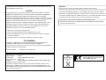
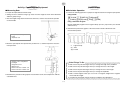
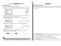
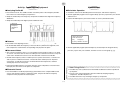
Connector SB-62
EA-200 to Power Graphic Unit
Declaration of Conformity
Model Number:
EA-200
Trade Name:
CASIO COMPUTER CO., LTD.
Responsible party: CASIO, INC.
Address:
570 MT. PLEASANT AVENUE, DOVER, NEW JERSEY 07801
Telephone number: 973-361-5400
This device complies with Part 15 of the FCC Rules. Operation is subject to the
following two conditions: (1) This device may not cause harmful interference, and
(2) this device must accept any interference received, including interference that may
cause undesired operation.
CASIO ELECTRONICS CO., LTD.
Unit 6, 1000 North Circular Road,
London NW2 7JD, U.K.
0-1
English
Contents
–– English ––
Handling Precautions ............................................................................ 0-2
Natural Frequency and Sound .......................................................... 2-6-1
Unpacking ............................................................................................. 0-3
Column of Air Resonance and the Velocity of Sound ....................... 2-7-1
About the EA-200 ................................................................................. 0-3
Construction of the Musical Scale .................................................... 2-8-1
Before Using the EA-200 for the First Time .......................................... 0-3
Direct Current and Transient Phenomena ......................................... 2-9-1
AC Circuit ........................................................................................ 2-10-1
Chapter 1
Dilute Solution Properties ............................................................... 2-11-1
General Guide ......................................................................................1-1
Exothermic Reaction....................................................................... 2-12-1
Supported Calculator Models ...............................................................1-2
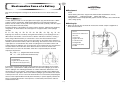
Electromotive Force of a Battery..................................................... 2-13-1
Supported Probes ................................................................................. 1-2
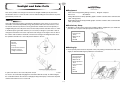
Sunlight and Solar Cells ................................................................. 2-14-1
Using Commands ................................................................................. 1-3
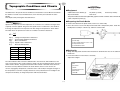
Topographic Conditions and Climate .............................................. 2-15-1
Using the Voltage Probe, Temperature Probe, Optical Probe,
and Motion Sensor (EA-2) .................................................................... 1-3
Program Library .................................................................. 2-16-1
Appendix A Command Tables
Using the Built-in Microphone ...............................................................1-4
Using the Built-in Speaker .................................................................... 1-5
Command 1 – Channel Setup .......................................................... α-1-1
Status Request ..................................................................................... 1-5
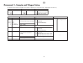
Command 3 – Sample and Trigger Setup ......................................... α-1-2
Auto Setup ............................................................................................ 1-5
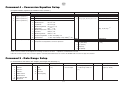
Command 4 – Conversion Equation Setup ....................................... α-1-3
Group Link Function .............................................................................1-6
Command 5 – Data Range Setup ..................................................... α-1-3
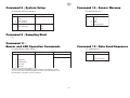
Command 6 – System Setup ............................................................ α-1-4
Chapter 2
Command 8 – Sampling Start .......................................................... α-1-4
Examples
Command 10 – Sensor Warmup ...................................................... α-1-4
Uniformly Accelerated Motion ........................................................... 2-1-1
Command 11 – Buzzer and LED Operation Commands .................. α-1-4
Period of Pendular Movement ........................................................... 2-2-1
Command 12 – Data Send Sequence .............................................. α-1-4
Conservation of Momentum .............................................................. 2-3-1
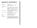
Appendix B Specifications ............................................... α-2-1
Charles’ Law ..................................................................................... 2-4-1
Polarization of Light .......................................................................... 2-5-1
20020601
0-2
English
• Never allow foreign objects to get into connector holes. Doing so can result in
malfunction.
Handling Precautions
• The EA-200 is made up of precision components. Never try to take it apart.
• Always make sure to connect probes only to their correct terminals. Never force the plug
of a probe into a wrong terminal connector.
• Avoid dropping the EA-200 and subjecting it to strong impact.
• Be sure to turn the EA-200 off before connecting or disconnecting probes.
• Do not store the EA-200 or leave it in areas exposed to high temperatures, humidity, low
temperatures, or large amounts of dust. Low temperatures can shorten battery life.
• Make sure that probes are connected securely before using them to take samples.
• Replace the main batteries once every two years regardless of how much the EA-200 is
used during that period. Never leave dead batteries in the battery compartment. They
can leak and damage the unit.
• Never insert a probe into an electric outlet. Never attempt to measure high voltages or
household AC. Doing so creates the danger of electric shock.
• Never apply more than 15V to analog channels CH1 or CH2, more than 5V to analog
channel CH3, or more than 5.5V to the SONIC, DIG IN, or DIG OUT channels. Doing so
can damage the EA-200.
• Keep batteries out of the reach of small children. If swallowed, consult with a physician
immediately.
• Avoid using volatile liquids such as thinner or benzine to clean the unit. Wipe it with a
soft, dry cloth, or with a cloth that has been dipped in a solution of water and a neutral
detergent, and wrung out.
• The EA-200 is to be used for educational purpose only. It is not appropriate for
industrial, research, medical, or commercial applications.
• In no event will the manufacturer and its suppliers be liable to you or any other person
for any damages, expenses, lost profits, lost savings or any other damages arising out of
loss of data and/or formulas arising out of malfunction, repairs, or battery replacement.
The user should prepare physical records of data to protect against such data loss.
• Never dispose of batteries, or other components by burning them.
• Replace batteries as soon as possible after the low battery indicator lamp (Batt) lights.
• Be sure that the power switch is set to OFF when replacing batteries.
• If the EA-200 is exposed to a strong electrostatic charge, its memory contents may be
corrupted or the keys may stop working. In such a case, perform the Reset operation to
clear memory contents and restore normal key operation.
• If you start to experience serious operational problems with the EA-200, use a thin,
pointed object to carefully press the P button on the back of the EA-200. Note, however,
that pressing the P button deletes all data currently in EA-200 memory. Proper operation
does not resume after you press the P button, remove its batteries, and then replace
them correctly in accordance with the instructions on page 0-3 of the User’s Guide.
• Note that strong vibration or impact during program execution can cause execution to
stop or can corrupt EA-200 memory contents.
• Using the EA-200 near a television or radio can cause interference with TV or radio
reception.
• Before assuming malfunction of the EA-200, be sure to carefully reread this User’s
Guide and ensure that the problem is not due to insufficient battery power, programming
or operational errors.
20020601
20020701
0-3
English
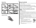
Unpacking
EA-200
About the EA-200
Soft case
The EA-200 is a digital device that makes it possible for you to sample data connected with
everyday natural phenomena.
Data communication cable
(SB-62)
Data You Can Sample with the EA-200
Temperature probe
Optical probe
Various different sensors can be used with the EA-200 to sample temperatures, light,
voltage, distance, and other data. The EA-200 supports sampling of up to 120,000 points,
and simultaneous sampling over five channels. Sampled data can be sent to a compatible
Graphic Scientific Calculator, where it can be viewed and graphed.
Voltage probe
Before Using the EA-200 for the First
Time
Four AA-size alkaline batteries
AC adaptor
User’s Guide (this manual)
Power Requirements
EA-200
Your EA-200 requires four AA-size alkaline batteries for power. Battery life depends on the
amount of time the EA-200 is left on, and the amount of current used by the connected
probe(s). A low battery indicator lamp (Batt) lights to let you know when it is time to replace
batteries. To extend battery life, it is a good idea to use the AC adaptor for power whenever
sampling indoors.
When using the EA-200 in combination with the optional “Motion Sensor (EA-2)”, be sure to
power the EA-200 using its bundled AC adaptor (AD-A60024).
Though the EA-200 can normally operate on battery power, separate AC adaptor power is
required while the optional “Motion Sensor (EA-2)” is being used.
Batteries are not loaded in the EA-200 when it is shipped from the factory. Because of this,
use the following procedure to load batteries into the EA-200 before using it for the first time.
User’s Guide
E
http://world.casio.com/edu_e/
Using the Soft Case
2
1
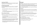
To load batteries
1. Remove the battery cover by pulling with your finger at the
point marked 1. If there are batteries in the battery
compartment, remove all four of them.
2. Load four new AA-size batteries. Make sure that the plus and
minus ends of the batteries are facing in the directions shown
by the markings inside the battery case. Replace the battery
cover.
3. Slide the [ON/OFF] switch to turn on the EA-200. To turn off,
slide the [ON/OFF] switch again.
20020601
1
0-4
English
Auto Power Off (APO)
AC Adaptor
Warning!
To extend battery life, power automatically turns off if you do not perform any operation for
about 30 minutes. APO is disabled automatically whenever the EA-200 is standing by for
sampling (ready state), or while sampling is in progress.
• Make sure the voltage of the power supply you are connecting to matches that of the
rating marked on the EA-200. Do not overload extension cords and wall outlets. Failure
to follow these precautions creates the danger of fire and electric shock.
• Never allow the power cord to become damaged, cracked, or broken. Never modify the
power cord in any way, and never subject it to excessive twisting or pulling. Never place
heavy objects on power cord and do not expose it to direct heat. A damaged power cord
creates the danger of electric shock.
Extended Sampling Mode
The Extended Sampling Mode makes it possible to sample data over an extended period
when operating under battery power. The following are the features of the Extended
Sampling Mode.
• Never touch the AC adaptor while your hands are wet. Doing so creates the danger of
electric shock.
• In the Extended Sampling Mode, sampling continues even though the power lamp is not
lit.
Caution!
• The Extended Sampling Mode is entered automatically whenever the sampling interval
is five minutes or longer.
• Always grasp the adaptor box and never pull on the power cord when unplugging the AC
adaptor. Doing so runs the risk of damaging the cord and creating the danger of fire and
electric shock.
• To exit the Extended Sampling Mode, press the [START/STOP] key. Note that all other
keys are disabled in the Extended Sampling Mode.
• Be sure to always unplug the AC adaptor whenever leaving the EA-200 unattended for
long periods.
• Use only the special AC adaptor that is specified for the EA-200.
• Use of any other type of AC adaptor creates the risk of serious problems with and
damage to the EA-200 and/or AC adaptor. Never use another type of AC adaptor. Note
that any damage due to use of the wrong type of adaptor is not covered by your
warranty.
When to Replace Batteries
Replace batteries as soon as possible after the low battery indicator lamp (Batt) lights. The
EA-200 may start to malfunction if you continue to use it while battery power is low.
• Make sure you turn off the EA-200 before connecting the AC adaptor.
• Be sure to replace the batteries at least once every two years, no matter how much you
use the EA-200 during that time.
• The AC adaptor may become warm if you use it for a long time. This is normal and does
not indicate malfunction.
• The batteries that come with this EA-200 discharge slightly during shipment and
storage. Because of this, they may require replacement sooner than the normal
expected battery life.
To connect the AC adaptor to the EA-200
1. Slide the [ON/OFF] switch to turn off the EA-200.
• Before removing the batteries, make sure you make a separate copy of sample data by
transferring it to a Graphic Scientific Calculator or some storage device. Cutting off all
power to the EA-200 by removing its batteries while the AC adaptor is not connected
causes all of the data in memory and all settings to be cleared.
2. Plug the AC adaptor into the port on the lower left of the EA-200.
3. Plug the other end of the AC adaptor into a wall outlet.
4. Slide the [ON/OFF] switch to turn on the EA-200.
• Whenever performing a sampling operation that requires more than a few minutes, we
recommend that you power the EA-200 using the AC adaptor. This will help to ensure
stable sampling operations.
20020601
1-1
English
Chapter 1
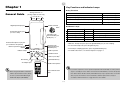
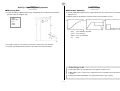
Key Functions and Indicator Lamps
Key Functions
General Guide
Analog Channels × 3
(Analog output for CH3 only)
CH3
CH2
CH1
Digital input/output port
Press this key:
Start a sampling operation from the ready state
[START/STOP]
Stop an ongoing sampling operation
[START/STOP]
Use Auto Setup (See “Auto Setup” on page 1-5.)
[SET UP]
Cancel the ready state
[SET UP]
Indicator Lamps
SONIC Channel
EA-2*1
0
Mo
tion
Sens
o
To do this:
When this indicator lamp:
Does this:
It means this:
Power (Green)
Lights
Power is on.
EA-200 is standing by for data (ready state).
10
180
Serial 232C (9-pin) port
(for cross cable)
Calculator 3-pin
communication port
(SUB port) × 7
External microphone 2-pin port
(for condenser microphone)
Lights
Flashes
Error (Red)
Lights
An error occurred.
Batt (Red)
Lights
It is time to replace the batteries.
Sampling is in progress.
• While the “Ready” lamp is lit, press the [START/STOP] key to start sampling.
Calculator 3-pin
communication port
(MASTER port)
External speaker 2-pin port
Volume
Indicator lamps
Ready (Green)
Sampling (Green)
Ready Sampling Error
Batt
• To cancel the ready state, press the [SET UP] key.
• To interrupt a sampling operation, press the [START/STOP] key.
Power
• For details about errors, see “Status Request” on page 1-5.
Built-in speaker
ON/OFF switch
SET UP
SET UP key
START/STOP
P button (rear side)*2
START/STOP key
AC adaptor port
Built-in microphone
1
* When using the EA-200 in combination
with the optional “Motion Sensor (EA-2)”,
*2 If you start to experience serious operational problems with the EA-200, use a thin, pointed
Data communication
cable
object to carefully press the P button on the back of the EA-200. Note, however, that pressing
the P button deletes all data currently in EA-200 memory. Proper operation does not resume
be sure to power the EA-200 using its
after you press the P button, remove its batteries, and then replace them correctly in
bundled AC adaptor (AD-A60024).
accordance with the instructions on page 0-3 of the User’s Guide.
20020601
1-2
English
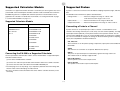
Supported Calculator Models
Supported Probes
Connection to a supported scientific calculator is essential if you want to get the most out of
your EA-200. A connected Graphic Scientific Calculator sends commands that control the
EA-200 during transfer of sampled data and other operations. Transferred data can be
graphed on the calculator. For details about commands, see “Using Commands” on page
1-3, and “Command Tables” on page α-1-1.
A probe is a sensor that connects to the EA-200 for sampling temperature, light, and other
data.
The EA-200 comes with the three probes described below.
• Voltage Probe ................... Measures voltage in the range of –10V to +10V.
CH3 measures in the range of –5V to +5V.
• Optical Probe ................... Measures luminance in the range of 100 to 999.
Supported Calculator Models
• Temperature Probe .......... Measures temperature in the range of –20°C to 130°C.
ALGEBRA FX Series
CFX-9850/fx-7400 Series
ALGEBRA FX 2.0 PLUS
CFX-9950GB PLUS
Connecting a Probe to a Channel
ALGEBRA FX 2.0
CFX-9850GB PLUS
FX 1.0 PLUS
CFX-9850Ga PLUS
FX 1.0
CFX-9850G PLUS
A probe connects to an input/output port called a “channel.” The EA-200 has seven
channels: three analog channels (CH1, CH2, CH3), one sonic channel (SONIC), one digital
input/output channel (DIG I/O), a microphone channel, and a speaker channel. You can
connect probes individually, or you can connect multiple probes for simultaneous sampling.
You can use commands to configure the settings for the channel being used for sampling, to
specify how sampled data should be handled, etc.
CFX-9970G
fx-9750G PLUS
CFX-9950G
CFX-9850G
CH1, CH2, CH3
fx-7400G PLUS
These channels are for the probes (voltage, temperature, optical) that come bundled with
the EA-200.
SONIC
This channel is for connection of an optional “Motion Sensor (EA-2)”.
fx-7450G
DIG I/O
This port is for input and output of an 8-bit binary signal in the range of 0V to 5V.
This could be used, for example, to light an LED.
Connecting the EA-200 to a Supported Calculator
Use the special data communication cable to connect the EA-200 to a supported Graphic
Scientific Calculator model.
Built-in Microphone
The microphone can be used to sample sound.
(1) Turn off the EA-200 and the calculator.
(2) Connect one end of the special data communication cable to the scientific calculator.
Built-in Speaker
The speaker can be used to output sound samples.
(3) Connect the other end of the cable to the EA-200’s MASTER port.
• Insert the plugs as far as they will go. If you experience problems when transferring data,
check to make sure that both plugs are fully inserted.
• Be sure to read the user documentation that comes with the scientific calculator you are
connecting.
20020601
1-3
English
Sending a Command
Using Commands
Example 1: To initialize the EA-200 setup
Basically, the EA-200 is controlled by commands from the connected calculator. This section
explains how to send commands from the calculator to the EA-200.
To use a command, you store parameters as List data on the calculator, and then use the
Send command to send the parameters to the EA-200.
_
{0} → List 1_
Stores {0} to List 1. 0 is the command number.
_
Send (List 1)_
Sending List 1 executes Command 0.
Example 2: To configure channel settings
_ Stores {1,1,2} to List 1. The first 1 is the command number, the
{1, 1, 2} → List 1_
second 1 is the channel number, and the 2 indicates use of the
voltage probe.
EA-200 Operation
The following is an outline of the EA-200 command receive process.
_
Send (List 1)_
1 Slide the EA-200 [ON/OFF] switch to turn on power.
2 EA-200 receives Command 0 sent from the calculator.
• This initializes the EA-200 setup.
Sending List 1 executes Command 1.
Receive Data Command
As with command execution, all of the operations required to receive data from the EA-200
to the calculator are performed on the calculator.
You can transfer sampled data by executing the calculator's Receive command.
Data is transferred in the sequence shown below.
Record Time → CH1 → CH2 → CH3 → SONIC
3 EA-200 receives Command 1 sent from the calculator.
• This configures EA-200 channel settings.
4 EA-200 receives Command 3 sent from the calculator.
• This configures EA-200 sampling conditions.
• After sampling conditions are configured, the EA-200 enters the ready state.
_ Stores transferred data into List 1 of the calculator.
Receive (List 1)_
5 Press the EA-200 [START/STOP] key.
• This puts the EA-200 into sampling mode.
• Sampling ends in accordance with the sampling conditions configured in step 4.
Using the Voltage Probe, Temperature
Probe, Optical Probe, and Motion Sensor
(EA-2)
6 Sample data is sent from the EA-200 to the calculator in response to a Receive
command.
The following examples show how to use the temperature probe, voltage probe, optical
probe, and “Motion Sensor (EA-2)”. Perform the procedures in each example by creating
programs on the calculator.
Taking 60 samples at one-second intervals over one minute
(1) Send Command 0 to initialize the EA-200 setup.
20020601
_
{0} → List 1_
Stores {0} to List 1. 0 is the command number.
_
Send (List 1)_
Sending List 1 executes Command 0.
1-4
English
(2) Send Command 1 to configure channel settings.
• Voltage Probe
(that is connected to CH1.)
_
{1, 1, 2} → List 1_
_
Send (List 1)_
The first 1 is the command number, the second 1 is the
channel number, and the 2 indicates use of the voltage
probe.
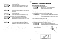
Using the Built-in Microphone
To take 255 samples at 50µs intervals
(1) Send Command 0 to initialize the EA-200 setup.
_
{0} → List 1_
_
Send (List 1)_
Stores {0} to List 1. 0 is the command number.
Sending List 1 executes Command 0.
• Temperature Probe
(that is connected to CH1.)
_
{1, 1, 7} → List 1_
_
Send (List 1)_
The first 1 is the command number, the second 1 is the
channel number, and the 7 indicates use of the temperature
(Celsius) probe.
(2) Send Command 1 to specify microphone as the channel.
• Optical Probe
(that is connected to CH1.)
(3) Send Command 3 to configure measurement condition settings.
_
{1, 1, 9} → List 1_
_
Send (List 1)_
The first 1 is the command number, the second 1 is the
channel number, and the 9 indicates use of the optical probe.
• Optional “Motion Sensor (EA-2)”
_
{1, 4, 2} → List 1_
_
Send (List 1)_
_
{1, 10} → List 1_
_
Send (List 1)_
(that is connected to SONIC channel.)
1 is the command number, 4 is the channel number
(SONIC), and 2 indicates use of the motion sensor (meters).
^
Send (List 1)^
{3, 0.00005, 255} →
_
List 1_
3 is the command number, 0.00005 is the sampling interval
(50µs), and 255 is the number of samples.
^
Send (List 1)^
You can change sampling conditions by using different
sampling interval and number of samples values, if you want.
At this time, the Ready lamp lights on the EA-200.
Press the EA-200 [START/STOP] key to start sampling.
When sampling is complete, press the calculator’s w key to restart the program.
^ (Disp command) causes processing to stop until you press the w key.
(3) Send Command 3 to configure measurement condition settings.
_
{3, 1, 60} → List 1_
1 is the command number, and 10 indicates use of
the built-in microphone.
3 is the command number, 1 is the sampling interval, and 60
is the number of samples.
You can change sampling conditions by using different
sampling interval and number of samples values, if you want.
(4) Sample data from the EA-200 is received by the calculator.
At this time, the Ready lamp lights on the EA-200.
Press the EA-200 [START/STOP] key to start sampling.
When sampling is complete, press the calculator’s w key to restart the program.
^ (Disp command) causes processing to stop until you press the w key.
_
Receive (List 1)_
Record Time data is received and stored in List 1.
_
Receive (List 2)_
Sampling Data of microphone is received and stored in List 2.
• When using the built-in microphone for sampling,
position it so it is about two or three centimeters
from the sound source.
(4) Sample data from the EA-200 is received by the calculator.
_
Receive (List 1)_
_
Receive (List 2)_
Record Time data is received and stored in List 1.
Sampling Data of CH1 is received and stored in List 2.
• If the graph shows that the sampled sound is exceeding the sampling range as
shown below, either lower the volume of the sound source or move the microphone
further away from the sound source.
20020601
1-5
English
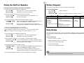
Using the Built-in Speaker
Status Request
To output sound recorded by the built-in microphone
This function can be used to fetch the current status of the EA-200.
(1) Send Command 0 to initialize the EA-200 setup.
To use Status Request
_
{0} → List 1_
Stores {0} to List 1. 0 is the command number.
_
{7} → List 1_
_
Send (List 1)_
Sending List 1 executes Command 0.
_
Send (List 1)_
_
Receive (List 1)_
(2) Send Command 1 to specify microphone as the channel.
_
{1, 10} → List 1_
_
Send (List 1)_
Line 1
Status
0: Standby
(No Sample Data in EA-200)
1: Ready
2: Sampling
3: Standby
(Sample Data in EA-200)
1 is the command number, and 10 indicates use of
the built-in microphone.
(3) Send Command 3 to configure measurement condition settings.
{3, 0.00005, 120000}
_
→ List 1_
3 is the command number, 0.00005 is the sampling interval
(50µs), and 120000 is the number of samples.
^
Send (List 1)^
You can change sampling conditions by using different
sampling interval and number of samples values, if you want.
At this time, the Ready lamp lights on the EA-200.
Press the EA-200 [START/STOP] key to start sampling.
When sampling is complete, press the calculator’s w key to restart the program.
^ (Disp command) causes processing to stop until you press the w key.
Stores {0} to List 1. 0 is the command number.
_
Send (List 1)_
Sending List 1 executes Command 0.
Receives the status information and stores it in List 1.
Line 2
Line 3
Line 4
Error Code
Battery Condition OS Version
= O: Normal
0 to 999
Version No.
≠ O: Error
Integer: Command number
< 450:
Decimal Part: Parameter position
low battery
Example: 3.2
Second parameter of Command 3.
Sampling interval value error
Auto Setup
Auto Setup detects the Auto-ID of a probe, and configures applicable settings automatically.
The three probes (voltage, temperature, optical) that come bundled with the EA-200 have
Auto-IDs.*1
(4) Send Command 0 to initialize the EA-200 setup.
_
{0} → List 1_
Sends Command 7.
To use Auto Setup
(5) After sampling is complete, use Command 1 to configure speaker settings.
1. Connect a probe to a channel.
_ 1 is the command number, 12 specifies the speaker as the
{1,12, 5,10} → List 1_
_
Send (List 1)_
channel, 5 is the number of loops, and 10 specifies output of
values sampled by the microphone.
2. Slide the [ON/OFF] switch to turn on power.
• This causes the Power lamp to light.
3. Press the [SET UP] key.
(6) Re-configure the sampling condition settings.
{3,0.00005,120000}
_
→ List 1_
3 is the command number, 0.00005 is the sampling interval
(50µs), and 120000 is the number of samples.
^
Send (List 1)^
You can change sampling conditions by using different
sampling interval and number of samples values, if you want.
• This causes the Ready lamp to light.
(7) Press [START/STOP] to output the sound recorded with the microphone.
*1 The optional “Motion Sensor (EA-2)” does not have an Auto-ID.
20020601
1-6
English
4. Press the EA-200 [START/STOP] key to start sampling.
Example Operation
The example below shows how a teacher can use the EA-200 Group Link function to
distribute a sampling program and sampled data.
• The Sampling lamp flashes as sampling is performed.
5. Press the [START/STOP] key again to stop sampling.
1. Students are divided into multiple groups, and each group has its own EA-200. The
teacher uses his or her EA-200 to distribute a sampling program to each of the group
leaders.
6. Connect the EA-200 to the calculator, and then use the Receive command to transfer
the sampled data (see the “Receive Data Command” on page 1-3).
• Data is transferred in the following sequence:
Record Time → SONIC →CH1 → CH2 → CH3.
Teacher Calculator
• Any channel that is not being used is skipped automatically.
Teacher EA-200
Group Leader 1 Calculator
Group Leader 2 Calculator
Group Link Function
Group Leader 3 Calculator
A single EA-200 can be used to connect one “MASTER” calculator to up to seven other
“SUB” calculators to distribute programs, data, etc.*1 Note, however, that you cannot have
the following calculator models connected to the EA-200 at the same time.*2
2. Each group uses the EA-200 to perform sampling using the program that was
distributed to the group leader’s calculator from the teacher’s calculator. After sampling
is complete, the EA-200 Group Link function is used to distribute the sampled data to
the calculator of each group member.
• ALGEBRA FX Series
• CFX-9850/fx-7400 Series*3
Group Leader Calculator
To perform a Group Link operation
Group EA-200
1. Use a Link Cable (SB-62) to connect the calculator that contains the data you want to
send to the MASTER port of the EA-200.
Group Member 1 Calculator
2. Use a Link Cable (SB-62) to connect the calculators to which you want to send the
data to the SUB ports of the EA-200).
Group Member 2 Calculator
3. Slide the [ON/OFF] switch of the EA-200 to turn it on.
Group Member 3 Calculator
4. On all of the SUB calculators, use the LINK application to enter the Receiving Mode.
Important!
5. On the MASTER calculator, use the LINK application to transmit the data.
• You can create your own sampling program while referring to the Program Library on
page 2-16-1, or you can download a program at the CASIO Website:
http://world.casio.com/edu_e/
6. The data transfer operation is over when the message “Complete” appears on the
displays of the MASTER calculator and all of the SUB calculators.
*1 Backup data cannot be distributed.
*2 See the “Supported Calculator Models” on page 1-2 for more information about compatibility
between various calculator models.
*3 fx-7400 Series calculators support Program and List data only.
20020601
Chapter 2
Examples
Uniformly Accelerated Motion
Period of Pendular Movement
Conservation of Momentum
Charles’ Law
Polarization of Light
Natural Frequency and Sound
Column of Air Resonance and the Velocity of Sound
Construction of the Musical Scale
Direct Current and Transient Phenomena
AC Circuit
Dilute Solution Properties
Exothermic Reaction
Electromotive Force of a Battery
Sunlight and Solar Cells
Topographic Conditions and Climate
Program Library
2-1-1
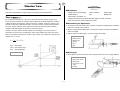
Uniformly Accelerated Motion
English
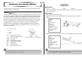
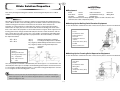
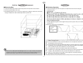
Activity: Setup
쐽 Equipment
This activity observes the movement of a cart down an incline and investigates uniformly
acceleration motion caused by gravity.
Cart
Ramp
Stand
Protractor
Distance Measurement Setup (EA-200, graphic scientific calculator, data communication
cable, optional EA-2*1)
Theory
쐽 Setting Up
A cart placed on an inclined ramp starts to move straight down the ramp. This movement is
due to the force of gravity acting on the cart to pull it down the incline and pulling it against
the ramp. The distribution of these two forces depends on the inclination of the ramp. The
acceleration of the cart is determined by the magnitude of the force that moves the cart.
Movement represented by an acceleration value that does not change over time is called
“uniformly accelerated motion.” The movement of the cart described above is uniformly
accelerated motion. As shown below, the velocity of uniformly accelerated motion is
proportional to time, and the distance traveled is proportional to the time squared. This
means that if you observe the distance covered by the cart over a specific time, you can
determine its acceleration.
u Affix the EA-2 to the arm of the stand.
u Measure the incline of the ramp with the protractor, and fix the ramp at an angle of 15
degrees.
1 Stand
2 Ramp
3 Desk
4 EA-2 (SONIC)
5 Protractor
6 Ramp Angle:
15 degrees
7 Distance from EA-2 to
end of ramp: 150cm
F = ma =mg sinθ
v = at
8 Ramp Width: 30cm
9 EA-200
L = 12 at 2
F (N)
a(m/s2)
m(kg)
g(m/s2)
θ (°)
v(m/s)
t(s)
L (m)
*1
u Measure the mass of the cart, place it onto the ramp, and hold it in place with your hand.
: Force Acting on Cart in
Direction of the Ramp Surface
: Cart Acceleration
: Cart Mass
: Gravitational Acceleration
: Ramp Angle of Inclination
: Cart Velocity
: Cart Travel Time
: Distance Traveled by Cart
1 Desk
2 Ramp
3 EA-2 (SONIC)
4 Cart Mass:
m(kg)
5 Distance Between Cart
and EA-2: 60cm
6 Protractor
7 Ramp Angle: 15 degrees
8 Hand
Though actual gravitational acceleration depends on latitude and elevation, this activity can be
conducted using the gravitational constant 9.8m/s2.
* 1 When using the EA-200 in combination with the optional ‘‘Motion Sensor (EA-2) ”, be sure to
power the EA-200 using its bundled AC adaptor (AD-A60024).
20020601
2-1-2
English
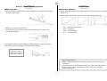
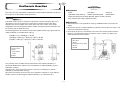
Measurement
Activity: Operating the Equipment
쐽 Measuring Data
쐽 Calculator Operation
u Prepare the Distance Measurement Setup. Immediately after starting the measurement
operation, let the cart go.
u Find the applicable program in the Program Library (P.2-16-1), input it into your calculator,
and then run it.
u Display graphs for the distance traveled, velocity, and acceleration of the cart.
L(m) : Distance Traveled by Cart
v(m/s) : Cart Velocity
a(m/s2) : Cart Acceleration
t(s)
: Cart Travel Time
u When the cart reaches the desk, stop it.
u Graph the data on the calculator, observe its characteristics, and compare it with
theoretical expectations.
u Change the angle of the ramp 10 degrees and then 20 degrees, and measure again.
u Observe how the graph changes as the ramp angle is changed.
1 Protractor
2 Ramp Angle: 15 degrees
3 Ramp Angle: 10 degrees
4 Ramp Angle: 20 degrees
u Study the relationships between the changes of distance traveled, velocity, and
acceleration.
u Consider the reasons why the graphs change as the angle of the ramp is altered.
u Find out how the graph is affected when the mass of the cart is changed by
placing a weight on it.
55555
55555
Other Things To Do
55555555555555555555555
5555555555555555555555
20020601
2-2-1
Period of Pendular Movement
English
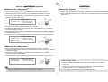
Activity: Setup
쐽 Equipment
In this activity, we create a simple pendulum and then visually check the periodicity of its
movement, while determining its period.
String with little elasticity Weight
Stand
Height adjustment blocks (2)
Optical Measurement Setup (EA-200, graphic scientific calculator, data communication
cable, optical probe)
Theory
쐽 Building a Pendulum
A pendulum is a string whose one end is fixed and whose other end has a weight attached
to it. As the weight swings, it keeps returning to the same position at the same velocity over
time. Such motion is called “periodic motion,” and the time it takes for the weight to return to
a particular state is called its “period.” A high-precision pendulum can continue to swing for
a very long time with little change in its period over time. This is why such a pendulum is
often used for timepieces.
A pendulum that moves across a single plane is called a simple pendulum. When the
amplitude of the pendulum is sufficiently short in relation to its length, the period of a simple
pendulum can be expressed as shown below.
u Securing the fixed point of the pendulum so it cannot move, assemble the pendulum as
shown in the illustration.
1 Stand
2 Pendulum Length: 30cm
3 Fixed Point
4 String
5 Weight: 100g
6 Weight Size: 3cm
7 Height: 2cm
8 Desk
T = 2π R
g
쐽 Setting Up
R(cm) : Pendulum Length
g(cm/s2) : Gravitational Acceleration
m(g)
: Mass of Weight
T(s)
: Period
u Align the heights of the optical probe and flashlight so the flashlight is shining directly at
the probe.
u Set up the pendulum so the weight blocks the light to the optical probe when it is at rest.
1 Fixed Point
All of this means that if gravitational acceleration is a fixed value that depends on the
location where the activity is performed, then the period depends on the length of pendulum
only.
With this activity, a pendulum is setup between a light source and an observer. The shadow
created by the weight makes it possible to observe the periodicity of the pendular motion.
1 Flashlight
2 Optical Probe (Observer) (CH1)
3 EA-200
Though actual gravitational acceleration depends on latitude and elevation, this activity can be
conducted using the gravitational constant. When gravitational acceleration is 980cm/s2 and
the length of the pendulum is 25cm, the oscillation period of the pendulum is about one second.
4 Distance Between Weight and Optical Probe: 10cm
5 Desk
20020601
2-2-2
English
Measurement
Activity: Operating the Equipment
쐽 Measuring Data
쐽 Calculator Operation
u Prepare the Optical Measurement Setup.
u Perform the following operation to prepare for light measurement using the optical probe.
u Taking care not to allow the string to go slack, move the weight as shown in the illustration
and then gently let it go.
Using E-CON
m“E-CON”w1(SETUP)b(Wizard)w
u After the weight swings back and forward a few times, start the measurement operation
on the EA-200.
1(CASIO)d(Light) 0.01w255w1(YES)
Using a Calculator Program
Find the applicable program in the Program Library (P.2-16-1), input it into your calculator,
and then run it.)
u Determine the period from graphs of the measurement results obtained at each
measurement position.
1 Weight Position of Equilibrium
2 Hand
3 Amplitude: 3cm
u Move the optical probe from position A to position B or C, and then repeat the measurement operation.
L : Light Intensity
t(s) : Time
T(s) : Period
1 Weight Position of Equilibrium
5555555
3 Weight Movement
4 Optical Probe
5 Distance Between A and B: 1cm
6 Distance Between A and C: 3cm
u Determine the period from the graph of measurement results, and compare this with the
calculated value.
u Find out how the period changes when you change the length of the pendulum.
u Find out how the period changes when you change the mass of the weight.
u Find out how the period changes when you change the size of the weight.
u Find out how the period changes when you change the amplitude.
5555555
Other Things To Do
55555555555555555555555
2 Flashlight
u Find out what happens when you use an iron or magnetic weight with a magnetic
sheet under the weight.
u Consider why the period changes under the conditions described above.
5555555555555555555555
20020601
2-3-1
Conservation of Momentum
English
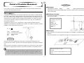
Activity: Setup
쐽 Equipment
The purpose of this activity is to investigate the law of conservation of momentum through
the collision of two carts.
Two carts of identical mass
String
Pulley with a bracket to secure it
Velcro쑓
500g weight
Cushion
Distance Measurement Setup (EA-200, graphic scientific calculator, data communication
cable, optional EA-2*1)
Theory
Collisions can take on many different forms, and can involve automobiles, locomotives,
shopping carts, or even two people. The force of the impact when the two objects collide
depends not only on their velocities but also their respective masses (weight), and you can
calculate the momentum of an object by multiplying its mass by its velocity.
Despite the variables involved, one principle always holds true – if external forces such as
friction are ignored, the sum of the momenta of two objects prior to collision is the same as
the sum of the momenta of the objects after collision. This is the principle known as the
“conservation of momentum.” This principle is an excellent tool for understanding the
dynamics of collisions.
The following expresses conservation of momentum in the case of a stationary cart being
struck by another cart, after which the two carts adhere to each other and continue in
motion together.
쐽 Preparing the Carts
u Measure the masses of Cart 1 and Cart 2.
u Affix Velcro쑓 to the impact surfaces of Cart 1 and Cart 2.
u Use tape to securely affix the string to the center of the front end (the same end where
the Velcro쑓 is affixed) of Cart 1.
1 Back of Cart 1
2 String
3 Velcro쑓
쐽 Setting Up
u Align the EA-2, Cart 1, Cart 2 and the pulley in a straight line.
m1v1 = (m1 + m2)v2
u Run the string under Cart 2 and place it onto the pulley. Attach the weight to the end of
the string.
m1(kg) : Mass of Cart 1
m2(kg) : Mass of Cart 2
v1(m/s) : Velocity of Cart 1 Before Collision
v2(m/s) : Velocity of Two Carts After Collision
u Support the weight with your hand so it does not pull Cart 1.
1 Cart 1
9 Distance: 50cm
2 Cart 2
0 Height of weight
3 Pulley
*1
from floor: 30cm
4 500g weight
! Desk
5 String
@ Floor
6 Cushions
# Velcro쑓
7 EA-2 (SONIC) $ EA-200
8 Allow 60cm
between EA-2
and Cart 1.
This means that when the two carts are of identical mass, the combined velocity of the two
carts after collision is one half that of the velocity of Cart 1 before the collision.
The above expression can be used to obtain the post-collision velocity of two carts (while they
adhere to each other) of different masses.
*1 When using the EA-200 in combination with the optional ‘‘Motion Sensor (EA-2) ”, be sure to
power the EA-200 using its bundled AC adaptor (AD-A60024).
20020601
2-3-2
English
Measurement
Activity: Operating the Equipment
쐽 Measuring Data
쐽 Calculator Operation
u Prepare the Distance Measurement Setup. Immediately after starting the measurement
operation, allow the weight to drop.
u Find the applicable program in the Program Library (P.2-16-1), input it into your calculator,
and then run it.
u Display graphs for the distance traveled, velocity, and acceleration of Cart 1.
1 Hand
2 500g weight
3 Floor
4 String
5 Pulley
L (m) : Cart 1 Distance Traveled
v(m/s) : Cart 1 Velocity
a(m/s2) : Cart 1 Acceleration
t (s)
: Time
u Be ready to catch the carts with your hands if the cushion does not stop them.
u Compare calculated theoretical velocity values with your measured velocity.
u Think about why Cart 1 Acceleration never registers a value of zero.
55555
55555
Other Things To Do
55555555555555555555555
u Add weight to Cart 1 and Cart 2 to change their masses and find out how this affects
velocity.
u Think about what would happen if we replaced the Velcro쑓 with a spring.
5555555555555555555555
20020601
2-4-1
Charles’ Law
English
Activity: Setup
쐽 Equipment
This activity is designed to confirm Charles’ law through an actual experiment.
Syringe (with scale markings)
Plastic Container
Rubber Tube
Rubber Gasket
Clip
Mixing Stick
Warm Water, Cold Water, Ice
Temperature Measurement Setup (EA-200, graphic scientific calculator,
data communication cable, temperature probe)
Theory
Increasing the temperature of a gas causes the molecules that make up the gas move
faster. The pressure within the container that holds the gas is determined by the number of
collisions between the molecules and the walls of the container, and by the velocity of the
molecules when they collide with the walls. If pressure remains constant and temperature
increases, the gas expands, which reduces the number of molecular impacts with the
container walls and negates the increase in molecular velocity.
Charles’ Law states that the thermal expansion of rarified gas of constant pressure is
proportional to the increase in temperature, and is represented by the expression shown
below. If the temperature when the volume of gas reaches zero is defined as absolute zero,
absolute zero is – 273°C.
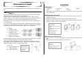
쐽 Assembling the Equipment
u Cut a hole into the side of the plastic container, and affix the rubber gasket around the
hole on the outside of the container.
u Slip the syringe with the rubber tube on its tip into the hole, and pack it with rubber to
make it watertight.
u Affix the clip to the rubber tube to seal the air inside the syringe.
1 Plastic Container
2 Rubber Gasket
V = V0 (T + 273)
3 Rubber Tube
273
4 Syringe
5 Hole
V (m3) : Gas Volume
V 0(m3) : Gas Volume at 0°C
T (°C) : Gas Temperature
6 Clip
쐽 Setting Up
1 Absolute Zero
u Fill the plastic container with warm water and wait until the air in the syringe stabilizes.
1 Plastic Container
2 Warm Water: 60°C
3 Mixing Stick
4 Temperature Probe
(CH1)
5 EA-200
20020601
2-4-2
English
Measurement
Activity: Operating the Equipment
쐽 Measuring Data
쐽 Calculator Operation
u The water temperature is displayed on the calculator.
u Use the Temperature Measurement Setup to measure the temperature and then display it.
u Read the volume of the gas using the markings on the syringe and
read temperature at that time, which is displayed on the calculator.
u Find the applicable program in the Program Library (P.2-16-1), input it into your calculator,
and then run it.
1 Temperature Probe
2 Mixing Stick
3 Syringe
4 Warm Water
5 Reading Position
u Add a little of the cold water to the water in the container, and mix. After waiting a few
minutes, take readings of the volume and temperature.
u Repeat this step until the temperature of the water in the container approaches the
temperature of the cold water.
1 Cold Water
2 Mixing Stick
u Repeat the above steps, adding ice instead of cold water and taking readings.
1 Ice
2 Mixing Stick
u Graph the readings, which produces a graph that is virtually linear.
u Substitute two of the values on the graph into the expression, and calculate the
temperature where volume becomes zero.
V = V1 – V0 T + V0
T1
T = – V0T1
V1 – V0
Should the plastic container become too full during the above steps, it is all right to remove some
of the water. However, make sure that the syringe remains under the surface of the water.
u See if you can approximate a linear graph where a large number of measured
values (plots) pass the point at –273°C (absolute zero).
u Consider why observed values are scattered around a straight line.
u Try repeating the above steps with the syringe filled with another type of gas
(helium, oxygen, etc.).
55555
55555
Other Things To Do
55555555555555555555555
5555555555555555555555
20020601
2-5-1
Polarization of Light
English
Activity: Setup
쐽 Equipment
This activity investigates the relationship between reflection, refraction, and polarization of
light.
Polarizers (2)
Thick Paper
Wood
Penlight
Glass
Screen
Protractor
Optical Measurement Setup (EA-200, graphic scientific calculator, data communication
cable, optical probe)
Theory
Light is electromagnetic radiation that has the properties of transverse waves. Sunlight
includes transverse waves that oscillate in various directions.
A polarizer allows only light vibrating in a specific direction to pass, which means that
sunlight coming out the other side is vibrating in that direction. This is called “polarization of
light.” Stacking together two polarizers with their polarization directions oriented
perpendicular to each other “extinguishes” the light, which means that no light penetrates
the second polarizer.
The expression below represents the change in the amplitude of light passing through the
second polarizer. Since light quantity changes in proportion to the square of its amplitude,
the light passing through the second polarizer is darker than the original light.
쐽 Preparing the Polarizers
u Cut holes in three sheets of thick paper, and use the protractor to measure and mark
angles on one of them.
u Mark the polarizing direction on the polarizers, and cut out one as a circle.
u Affix the wood frame and blocks to the thick paper, sandwich the polarizer between the
two sheets of paper as shown in the illustration.
1 Wood Frame
2 Wood Blocks
3 Thick Paper with Hole Cut
Out
A’ = Acosθ
4 Arrow Indicating Polarizing
Direction
A’ : Amplitude of Light
5 Removable Polarizer
Polarized by Polarizer 2
A : Amplitude of Light
Polarized by Polarizer 1
θ (°) : Angle of Polarization
Direction of Two Polarizers
6 Circular Polarizer
7 Angle Markings
쐽 Preparing the Glass Stand
u Fix the screen one centimeter above the glass surface that will be struck by the incident
light.
Most light is polarized when it is reflected or refracted by the boundary surface of material
where electromagnetic fields meet the required boundary conditions.
Especially at an angle called “Brewster’s angle,” polarization is completely linear, and
reflected light and refracted light polarization is orthogonal. The expression shown below
defines the conditions that such an angle needs to satisfy.
α + β = 90°
u Affix the protractor in accordance with the screen position.
1 Glass
2 Screen
3 Protractor
1 Incident Light
α (°) : Angle of Incidence and
2 Reflected Light
Angle of Reflection
β (°) : Angle of Refraction
3 Refracted Light
4 Distance Between Screen
and Glass Surface: 1cm
4 Boundary
Surface
20020601
2-5-2
English
Measurement
Activity: Operating the Equipment
쐽 Measuring the Angle of Polarization and the Light Intensity
쐽 Calculator Operation
u Position the optical probe so it is pointing at the penlight and picking
up the maximum light intensity.
u Prepare for measurement of light intensity using the optical probe, which will let you
determine the angle of polarization.
u Prepare the Optical Measurement Setup and start the measurement. Rotate the polarizer
90 degrees at a constant speed, every 20 seconds.
1 Penlight
4
2
2 Polarizers
m“E-CON”w1(SETUP)b(Wizard)w
1(CASIO)d(Light) 0.1w200w1(YES)
4
Using a Calculator Program
5
3 Optical Probe (CH1)
4 Hand
Using E-CON
5 Polarizing Direction
Find the applicable program in the Program Library (P.2-16-2), input it into your calculator,
and then run it.
3
1
6
u This displays a graph that shows changes in light intensity as the polarizer is rotated.
6 Direction of Turn
7 EA-200
7
L : Light Intensity
t(s): Time
쐽 Measuring Brewster’s Angle
u The light intensity is displayed on the calculator.
u From an angle determined using the protractor, shine the penlight beam onto the glass.
u Position the optical probe so it is pointing at the light beam and picking up the maximum
light intensity.
u Perform the following operation to measure Brewster’s angle.
u Rotate the polarizer until the polarization direction is that where the light intensity is the
greatest.
u Find the applicable program (Light Multi Meter) in the Program Library (P.2-16-2), input it
into your calculator, and then run it to measure light intensity.
u Measure the polarizing direction of the reflected light.
u Measure the polarizing direction of the refracted light.
u Determine the angle of the penlight beam that satisfies the condition expression of
Brewster’s angle.
1 Penlight
2 Polarizer for Reflected Light Measurement
3 Optical Probe for Reflected Light
Measurement
4 Polarizer for Refracted Light Measurement
Measurement
To obtain an accurate picture of changes in polarizer angle and light intensity, it is a good idea to
graph light intensity at various angles.
u Investigate changes in Brewster’s angle using materials other than glass.
u The 3D effect is possible because of the slight difference between how an object is
viewed by the left and right eyes. Consider how 3D imaging technology uses the
characteristics of light polarization to achieve its effects.
55555
55555
Other Things To Do
55555555555555555555555
5 Optical Probe for Refracted Light
5555555555555555555555
20020601
2-6-1
Natural Frequency and Sound
English
Activity: Setup
쐽 Equipment
This activity investigates sounds produced in accordance with the natural frequencies of
objects we use in everyday life. It also studies the characteristics of frequencies.
Box
String
Bolts (2)
Triangular Wood Blocks (2)
Audio Measurement Setup (EA-200, graphic scientific calculator, data communication
cable)
Theory
쐽 Building a Monochord
Hitting, striking, plucking, or otherwise disturbing just about any object will cause it to
vibrate. Dropping a pencil or ruler to the floor, or plucking a banjo string will cause it to
vibrate. The sound produced when you blow over the top of a bottle is the air inside of it
vibrating. The vibration of an object tends to occur at a particular frequency or a particular
set of frequencies, which is the “natural frequency” of the object.
Though the strength of the strike, pluck, or other disturbance applied to an object affects the
frequency of the sound produced, in most cases the sound produced is a louder version of
the natural frequency. Generally, the sound produced by an object is the result of multiple
natural frequency sound waves superimposed on each other.
The expression below provides the natural frequency of a string that is fixed at both ends. In
this case, all of the natural frequencies are integer multiples of f1, which is called the
“fundamental frequency.” The fundamental frequency is the lowest possible frequency at
which an object can vibrate freely.
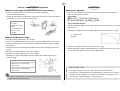
u Use tape to affix the bolts at either end of the box, and stretch the string taut between
them.
u Insert a triangular wood block between the string and the box.
1 Box
2 Box Length: 50cm
3 Bolt
4 String
5 Block
쐽 Setting Up
u Insert two wood blocks between the string and box, and set the monochord on a table or
desk.
n S
fn = 2L ρ
u Position the Audio Measurement Setup where it can pick up the sound from the
monochord.
fn (Hz) : String Natural Frequency (n = 1, 2, 3 ...)
L (m) : String Length
S (N)
: String Tension
ρ (kg/m) : String Linear Density (per meter)
1 Desk
2 Monochord
3 EA-200
20020601
2-6-2
English
Measurement
Activity: Operating the Equipment
쐽 Measuring the Sound Frequency
쐽 Calculator Operation
u Position the two wood blocks so there is about 40cm between them, and then lightly pluck
the center of the string to produce a sound.
u Prepare the Audio Measurement Setup for recording.
u Find the applicable program in the Program Library (P.2-16-2), input it into your calculator,
and then run it.
u Record the sound with the Audio Measurement Setup, perform FFT analysis, and view
the frequency distribution.
u Perform FFT analysis on the sound recorded when the blocks are 40cm apart, and study
the frequency distribution.
1 Monochord
2 Desk
1 Waveform
S
3 Distance Between
2 Frequency
t(s)
Blocks: 40cm
4 Finger
3 f 11
: Sound Volume
: Time
Distribution N(counts) : Number of
Counts
4 f 12
f (Hz)
: Frequency
u Position the two wood blocks so there is about 20cm between them, and then lightly pluck
the center of the string to produce a sound.
u Perform FFT analysis on the sound recorded when the blocks are 20cm apart, and study
the frequency distribution.
u Record the sound on the Audio Measurement Setup, perform FFT analysis, and view the
frequency distribution.
1 Monochord
1 Waveform
S
2 Frequency
t(s)
: Sound Volume
: Time
Distribution N(counts) : Number of
Counts
4 f 22
f (Hz)
: Frequency
2 Desk
3 f 21
3 Distance Between
Blocks: 20cm
4 Finger
u Calculate values for f12/f11, f22/f21, f21/f11, and compare them.
u Try changing the distance between the blocks, the location where you pluck the string,
and the strength of the pluck, and see how it affects the frequency.
u Consider the reason why f12/f11, f22/f21, and f21/f11 are values in the vicinity of 2.
u Consider the reason why f 12/f11, f22/f21, and f21/f11 are not exactly 2.
u Find out how the natural frequency changes when you use a different type of
string.
u Modify the monochord as shown in the illustration below, and adjust the weight so
it changes the tension of the string. Study how the natural frequency is affected by
changes in the tension of the string.
1 Pulley
2 Weight
55555555555
55555555555
Other Things To Do
55555555555555555555555
u Next, note the relationship with each of the above values with the value 2.
5555555555555555555555
20020601
2-7-1
Column of Air Resonance and
the Velocity of Sound
English
Activity: Setup
쐽 Equipment
Glass Resonance Tube (Uniform Inside Diameter, With Scale Markings)
Rubber Tube
Reservoir
Stand
Low Frequency Generator (or Tuning Fork)
Audio Measurement Setup (EA-200, graphic scientific calculator,
data communication cable)
Temperature Measurement Setup (EA-200, graphic scientific calculator,
data communication cable, temperature probe)
This activity uses the resonance of a column of air to measure the velocity of sound.
Theory
Resonance is what occurs when one object vibrating at the same natural frequency of a
second object causes the second object to vibrate. If you have two tuning forks of the same
natural frequency located near each other and strike one of the tuning forks so begins
vibrating, the other tuning fork will also vibrate even if you do not strike it. This is due to
resonance.
This activity uses a fixed-frequency sound source to produce resonance in a vertical
resonance tube. The sound produced by the resonating column of air will sound louder than
the sound produced by the sound source.
The expressions below show the relationships between the length of the column of air and
wavelength, and the velocity of sound and wavelength. The relationship between the
velocity of sound and wavelength is called the basic equation.
쐽 Setting Up
u Set up the equipment as shown in the illustration, and fill with water, taking care it does
not overflow.
u Raise and lower the reservoir and check to make sure that the level of the water changes.
1 Glass Resonance Tube
2 Tube Length: 1 meter
3 Stand
4 Reservoir
Ln = 2n–1 λ – 욼L v = f λ
4
5 Rubber Tube
6 Low Frequency Generator:
800Hz
L n(m) : Air Column Length for Resonance
Point n (n = 1, 2, 3...)
욼L (m) : Air Column Open-end Correction
λ (m) : Wavelength of Sound
v(m/s) : Velocity of Sound
f(Hz) : Frequency of Sound Wave
7 Speaker
8 EA-200
1 Resonance Point 1
2 Resonance Point 2
Actually, the air around the opening in the resonance tube also behaves like part of the air
column. This is called “open-end correction.” The effects of open-end correction can be
eliminated by measuring the length of the air column at Resonance Point 1 and Resonance
Point 2 and calculating the difference between the two. This can be used in combination
with the wave basic equation to determine the velocity of sound, using the expression
below.
v
20020601
2-7-2
English
Measurement
Activity: Operating the Equipment
쐽 Measuring the Resonance Points
쐽 Calculator Operation
u Record the sound on the Audio Measurement Setup,
display the waveform, and observe the amplitude.
u Use the Audio Measurement Setup to record the sound and display the waveform.
u Find the applicable program in the Program Library (P.2-16-2), input it into your calculator,
and then run it.
u Lower the water level, and find the point of maximum
amplitude.
Waveform
Amplitude
S :Sound Volume
t(s):Time
1
1 Glass Resonance Tube
2 Resonance Point 1
3 L1
A: Water Level A
B: Water Level B
C: Water Level C
2
4 Sound Wave Amplitude
u Lower the water level more, and find the next point of
maximum amplitude.
1 Glass Resonance Tube
2 Resonance Point 1
3 L1
Waveform at Water Levels A, C, D, and F
D: Water Level D
E: Water Level E
F: Water Level F
u Confirm that amplitude is at its maximum
for water levels B and E.
4 Resonance Point 2
5 L2
6 Sound Wave Amplitude
u Repeat the measurement three times and calculate
the average of the results.
Waveform at Water Levels B and E
u Substitute the average values of L1 and L2 into the
theoretical expression and calculate the velocity of
sound.
u Use the temperature probe to measure the temperature and then display it.
쐽 Measuring the Temperature of the Air Column
Other Things To Do
55555555555555555555555
u Find the applicable program (Charles’ Law) in the Program Library (P.2-16-1), input it into
your calculator, and then run it.
u Substitute the measured temperature values into the expression and calculate the
velocity of sound. Next, compare the results with the previously obtained value.
v = 331.5 + 0.61T
v(m/s) : Velocity of Sound
T (°C) : Air Column Temperature
1 Glass Resonance Tube
2 Temperature Probe (CH1)
3 EA-200
u Repeat the experiment using a different frequency, and compare the difference in
resonance points and sound velocity.
u Use FFT analysis to determine the frequency at each water level, and compare the
results with the sound source frequency.
u Substitute the observed velocity into the theoretical formula and calculate the openend correction value.
u Investigate what you need to multiply the open-end correction value in order to
obtain the inside diameter of the resonance tube.
u Perform the activity with a glass tube of a different diameter and find out how the
open-end correction value is affected.
5555555555
5555555555
u Use the Temperature Measurement Setup to measure the temperature and then display it.
5555555555555555555555
20020601
2-8-1
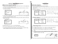
Construction of the Musical Scale
English
Activity: Setup
쐽 Equipment
The purpose of this activity is to investigate the scale that is most commonly used for
Western-style music, and to listen to some of the consonance it can produce.
Piano (Sound Source) Computer (MIDI Sound Source)
Audio Measurement Setup (EA-200, graphic scientific calculator, data communication
cable)
Theory
쐽 Setting Up
The pitch of a note is determined by its frequency, and the human ear perceives notes as
differences in frequency ratios, rather than differences in the relative amplitude of the
frequency.
The ratios of the 12-note mean scale used for most Western-style music is governed by a
number of restrictions. First, the frequency ratio of the same note from one octave to the
next is 2:1 (higher note to lower note). Each octave is divided into 12 parts, with the same
frequency ratio between each of the adjoining notes in the octave. The illustration below
shows each of the notes in an octave, on a piano keyboard.
u Take care so there is no unwanted noise in the area where you are conducting the activity.
1
1 Piano
2 Computer (MIDI
2
Sound Source)
3 EA-200
1 1 Octave (2:1 frequency ratio
between notes)
2 Tonic Note (Low Note)
3
3 Harmonic (High Note)
4 Adjacent Note (Note
Frequency Ratio = 2(1/12))
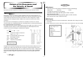
The frequencies of this 12-note scale can be expressed as shown below.
n
fn = 2 12 f 0
f 0(Hz) : Tonic Note Frequency
f 12(Hz): Harmonic Frequency
fn(Hz) : Frequency of nth Note (n = 1, 2, 3, ....12)
1 Frequency (Hz)
2 Low Note
3 High Note
Generally, notes consist of sound waves of different frequencies and amplitudes. Producing
two notes of different pitches at the same time sounds pleasing to the human ear, and such
notes are said to be “consonant.” Two notes whose frequency ratio is the ratio of two simple
integers are very consonant.
20020601
2-8-2
English
Measurement
Activity: Operating the Equipment
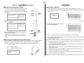
쐽 Analyzing Do-Re-Mi
쐽 Calculator Operation
u Record the notes Do, Re, and Mi, and then record the peaks of their frequency distributions. These are called “frequency components.”
u Record the sound on the EA-200, perform FFT analysis, and view the frequency.
u Find the applicable program in the Program Library (P.2-16-2), input it into your calculator,
and then run it.
u Study the relationship of the frequency components included in the single-note frequency
distribution.
u Use the EA-200 frequency conversion function to create synthesized sounds.
u Study the relationship of the highest peaks of different notes.
1 Waveform
2 Frequency
Distribution
1
2
3
3
3 Peak
1 Before Conversion
2 After Conversion
f (Hz)
: Frequency
N(counts) : Number of Counts
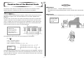
쐽 Octaves
u Record Do in two adjoining octaves, and make a note of its frequency components.
u On the EA-200, double the frequency of the lower Do to synthesize the higher Do, and
then compare the result with the corresponding note played on the piano.
u Find the applicable program (Natural Frequency and Sound) in the Program Library
쐽 Consonant Notes
(P.2-16-2) , input it into your calculator, and then run it to use FFT graph (1, 2).
u The sound at a frequency ratio of 1:1 is the original sound, and the sound at 2:1 is called
an “octave.” Two notes such as these are said to possess “absolute consonance.” Play the
same note in two different octaves to see what absolute consonance sounds like.
u Sounds at the frequency ratios 3:2 and 4:3 possess “perfect consonance,” sounds at 5:3
and 5:4 possess “medial consonance,” and sounds at 6:5 and 8:5 possess “imperfect
consonance” Predict the consonance of Do-Re-Mi from their frequencies, and then
actually play the notes on the piano.
u Using the EA-200’s frequency conversion function, create and produce consonant notes.
Next, play the same notes on the piano for comparison.
쐽 Electronic Sound
u Use the EA-200 to record Do played using a piano timbre on the computer MIDI sound
source, and check its frequency components. Next, compare this with the frequency
component of Do played on the acoustic piano.
u Consider why notes synthesized on the EA-200 are different from those produced
by the piano.
u In many cases, physical properties become evident by studying frequency
components. Consider why this is so.
u Consider what noise is by checking its frequency components.
55555
55555
Other Things To Do
55555555555555555555555
5555555555555555555555
20020601
2-9-1
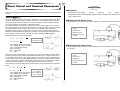
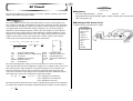
Direct Current and Transient Phenomena
English
Activity: Setup
쐽 Equipment
This activity investigates transient phenomena when direct current flows through a capacitor
and coil.
Battery (D.C. Power Supply)
Resistor
Capacitor
Coil
Switch
Voltage Measurement Setup (EA-200, graphic scientific calculator, data communication
cable, voltage probe)
Theory
Generally speaking, electrical current is the movement of free electrons within metal. When
electrical current flows through a capacitor, electrons are accumulated, and the capacitor
stores the charge. The accumulation of an electrical charge is called “charging,” while the
loss of the charge by the capacitor is called “discharging.”
Connecting a resistor and capacitor serial circuit to a D.C. power supply causes current to
flow to the capacitor, which charges until it reaches a steady state. Now if the power supply
is removed and the circuit is closed, current flows to the capacitor again, which now
discharges until it reaches a steady state. Current flows to the capacitor in the opposite
direction that it flowed during charging. The change in capacitor voltage during the transient
phase until the capacitor reaches a steady state, while charging and discharging is
represented by the expression shown below.
(
– t
RC
VC = V – VR = V 1– e
VC = V R = V e
)
– t
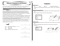
쐽 Building the RC Series Circuit
u The product of the resistance value and the capacitor’s capacitance should be around 1.
1 3V D.C. Power Supply
2 Switch
3 10kΩ Resistor
4 100µ F Capacitor
5 Voltage Probe (CH1)
6 EA-200
1 Charge Circuit
2 Discharge Circuit
RC
VR (V ): Voltage Across the Resistor
VC (V ): Voltage Across the Capacitor
V (V ) : Power Supply Voltage
R (Ω) : Resistance
C (F ) : Capacitance
t (s ) : Time
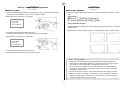
쐽 Building the RL Series Circuit
u The quotient when the resistance value is divided by the self-inductance of the coil should
be around 1.
1 3V D.C. Power Supply
When the current flowing through a coil changes over time, the coil induces voltage, like an
electrical generator. This is called “self-induced electromotive force,” which acts to oppose
the change in current. When a D.C. power supply is connected in a resistor and coil series
circuit, the effect of the coil’s self-induced electromotive force can be observed until current
reaches a fixed value. Similarly, self-induced electromotive force can also be observed by
cutting off the power supply to a circuit through which steady current is flowing.
The change in coil voltage during these transient phases is represented by the expressions
below.
VL = VR – V = – Ve
VL = VR = Ve –
2 Switch
3 0.1Ω Resistor
4 100mH Coil
5 Voltage Probe (CH1)
6 EA-200
– Rt
L
Rt
L
VR (V ): Voltage Across the Resistor
VL (V ): Voltage Across the Coil
V (V ) : Power Supply Voltage
R (Ω) : Resistance
L (H) : Self-inductance
t (s ) : Time
1 Circuit With
Power Supply
2 Circuit Without
Power Supply
20020601
2-9-2
English
Measurement
Activity: Operating the Equipment
쐽 Measuring Data
쐽 Calculator Operation
u Prepare the Voltage Measurement Setup. At the same time you start the measurement
operation, move the switch to “ON” to connect the power supply.
u Perform the following operation to prepare for voltage measurement using the voltage
probe.
u Wait until the circuit achieves a steady state.
Using E-CON
m“E-CON”w1(SETUP)b(Wizard)w
1 Switch
1(CASIO)b(Volt) 0.02w255w1(YES)
2 Power Supply
Connected
Using a Calculator Program
3 Power Supply Cut
Find the applicable program in the Program Library (P.2-16-3), input it into your calculator,
and then run it.
u Graph results for when the power supply is connected and for when it is disconnected.
u Prepare the Voltage Measurement Setup. At the same time you start the measurement
operation, move the switch to “OFF” to disconnect the power supply.
u Wait until the circuit achieves a steady state.
1 Switch
2 Power Supply
Voltage Change when Power Is Connected
Connected
3 Power Supply Cut
u Perform the above operation for the RC series circuit and the RL series circuit.
u Read and check the RC and R/L values from the graph.
Voltage Change when Power Is Disconnected
u It appears as if combining the curve during capacitor charging and the curve
during capacitor discharging will produce a straight line with no change over time.
This, however, is not necessarily so. Consider the reason for this.
u In the case of the coil voltage curves as well, it appears as combining them as
expressions should produce a straight line. However, this also does not happen.
Consider the reason for this.
u Change the resistor, capacitor, and coil and find out how the voltage is affected.
u While the capacitor is charged, cut off the power supply and observe changes in
capacitor voltage with the circuit left open. Compare what you observe with the
change in voltage when the circuit is closed.
555555555
555555555
Other Things To Do
55555555555555555555555
5555555555555555555555
20020601
2-10-1
English
AC Circuit
Activity: Setup
쐽 Equipment
This activity investigates the characteristics of a resistor, capacitor, coil (RCL) series circuit,
which is connected to an AC power supply.
AC Power Supply (Switched)
Resistor
Capacitor
Coil
Voltage Measurement Setup (EA-200, graphic scientific calculator, data communication
cable, voltage probe (3))
Theory
쐽 Building the RCL Series Circuit
The electrical power sent from power generating stations to homes is alternating current
(AC), not direct current (DC). Though direct current does not alternate with time, alternating
current alternates according to a regular cycle, and this cyclical change can be expressed
as a trigonometric function. When the voltage and frequency of a AC power supply are
defined, the current flowing through the circuit has the same frequency as but a different
phase from the power supply voltage. The phase difference and the magnitude of current
depends on the component parts of the circuit. The voltage and current when a AC power
supply is connected to a series circuit composed of a resistor, capacitor, and coil (RCL
series circuit) can be expressed by the expressions shown below.
V = V0 cosω t I = I0 cos(ω t – φ ) ω = 2πf
V0
I0 =
tan φ = 1 Lω – 1
R
Cω
2
1
R2 + Lω – ω
(
V (V )
:
V0 (V) :
I (A)
:
I0 (A)
:
ω (rad/s):
f (Hz) :
C
(
)
AC Power Supply Voltage
Amplitude of AC Power Supply Voltage
AC Current
Amplitude of AC Current
Angular Frequency
AC Frequency
u Build a circuit for a 3V, 50Hz power supply.
1 3V, 50Hz AC
Power Supply
2 10Ω Resistor
3 100µ F
Capacitor
4 10mH Coil
5 Voltage Probe
6 CH1
7 CH2
)
8 CH3
9 EA-200
R(Ω)
C(F)
L(H)
φ (rad)
t(s)
:
:
:
:
:
Resistance Value
Capacitor Capacitance
Coil Self-inductance
Current Phase Difference
Time
This activity investigates the voltage across the components of a series circuit. When a
current that alternates with time is applied, the voltage across a capacitor and a coil is out of
phase with the power supply voltage by -π/2 and π/2 respectively. The resistor does not
have this characteristic, and so there is no phase lag. All of this means the peaks and
valleys of the waveforms of the voltage across the components will be in different locations.
The voltage across each of the components is expressed as follows.
VR = I0R
I0
VC = C ω
VL = I0 Lω
VR (V) : Voltage Across the Resistor
VC (V) : Voltage Across the Capacitor
VL (V) : Voltage Across the Coil
We also know that the maximum current value is achieved using a capacitor-coil combination
that satisfies the conditions shown below. A frequency like this is called a “resonant frequency.”
ω2 =
1
LC
20020601
2-10-2
English
Measurement
Activity: Operating the Equipment
쐽 Measuring Data
쐽 Calculator Operation
u Check the values of the AC power supply, resistor, coil, and capacitor, and then switch on
the power supply.
u Perform the following operation to prepare for voltage measurement using the voltage
probe.
u Prepare the Voltage Measurement Setup and measure voltage.
Using E-CON
u Display and compare the change of voltage across each component.
m“E-CON”w1(SETUP)c(Advan)
b(Channel)1(CH1)c1(CASIO)b(Volt)c1(LIST) 2w
c2(CH2)c1(CASIO)b(Volt)c1(LIST) 3w
c3(CH3)c1(CASIO)b(Volt)c1(LIST) 4ww
c(Sample)1(NO)c1(TIMER) 0.001wc1(NUM) 255ww1(START)
Using a Calculator Program
Find the applicable program in the Program Library (P.2-16-3), input it into your calculator,
and then run it.
u Display VR , VC, and VL.
VR (V) : Voltage Across the Resistor (CH1)
VC (V) : Voltage Across the Capacitor (CH2)
VL(V) : Voltage Across the Coil (CH3)
t(s)
: Time
Make sure that the individual voltage value across the resistor, capacitor, and coil does not
exceed 5V. Consequently, you should make sure that the power supply voltage for the
combination shown here does not exceed 3V.
u Consider what type of combination would be required to keep voltage across all
parts below 5V.
u Consider combinations that satisfy conditions for resonance.
u Consider what component combinations would satisfy the conditions of this activity
(5V or less across each component, resonance circuit) for other AC frequencies.
u Perform FFT analysis and compare the frequency of each component.
555555
555555
Other Things To Do
55555555555555555555555
5555555555555555555555
20020601
2-11-1
Dilute Solution Properties
English
Activity: Setup
쐽 Equipment
Stand
Heater
Reflux Condenser
Desiccant
Auto Stirrer
Beaker
Round Bottom Flask (2)
Mixing Stick
Ice Water
Benzene
Naphthalene
Temperature Measurement Setup (EA-200, graphic scientific calculator, data
communication cable, temperature probe)
This activity investigates boiling point elevation and freezing point depression of a dilute
solution.
Theory
Dissolving a small amount of a substance (solute) in a theoretically pure liquid (solvent) to
create a dilute solution causes the boiling point of the dilute solution to become greater than
and the freezing point to become less than that of the solvent. This is because the
proportion of solvent molecules is reduced by the amount of solute molecules mixed in,
which lowers the vapor pressure of the solvent and elevates the boiling point. At the same
time, it also reduces the proportion of solvent molecules that congeal, which suppresses the
freezing point. These changes are determined by the amount of solute molecules, and the
type of solute does not matter, as long as it is non-volatile. Consequently, both boiling point
elevation and freezing point depression are proportional to the solute molality, as shown in
the expressions below.
욼T1 = K1 m
욼T2 = K2 m
쐽 Setting Up the Boiling Point Elevation Equipment
u Pour the benzene solution into the flask, and secure it in place as shown in the illustration.
1 Stand
2 Heater
3 Round Bottom Flask
4 Reflux Condenser
5 Desiccant
6 Naphthalene-Benzene
욼T1(°C)
:
욼T2(°C)
:
K1(°C kg/mol) :
K2(°C kg/mol) :
m(mol/kg)
Boiling Point Elevation of Solution
Freezing Point Depression of Solution
Molal Boiling Point Elevation Constant
Molal Freezing Point Depression
Constant
: Molality
Solution
7 Temperature Probe (CH1)
8 EA-200
9 Water Flow Direction
1 Solvent
2 Solution
쐽 Setting Up the Freezing Point Depression Equipment
3 Boiling Point Elevation
4 Freezing Point Depression
u Pour the benzene solution into the flask, and secure it in place as shown in the illustration.
T(°C) : Temperature
P(atm) : Vapor Pressure
t(s)
1 Stand
: Time
2 Auto Stirrer
3 Beaker
Here, the proportion coefficient is determined by the solvent type. It is a constant that is not
affected by the solute type. For example, the molal boiling point elevation constant for benzene
is 2.53°C kg/mol, and the boiling point is 80.1°C. The molal freezing point depression constant
is 5.12°C kg/mol, and the freezing point is 5.53°C.
4 Round Bottom Flask
5 Mixing Stick
6 Ice Water
7 Temperature Probe (CH1)
8 EA-200
When the solvent is pure water, the molal boiling point elevation constant is 0.515°C kg/mol,
and the boiling point is 100°C. The molal freezing point depression constant is 1.853°C kg/mol,
and the freezing point is 0°C.
20020601
2-11-2
English
Measurement
Activity: Operating the Equipment
쐽 Measuring Data
쐽 Calculator Operation
u
u
u
u
u Perform the following operation to prepare for temperature measurement using the
Temperature Measurement Setup.
Measure the mass of the beaker used for creating the solution.
Slowly pour the benzene into the beaker so it flows down the inside surface of the beaker.
Measure the mass of the small amount of naphthalene being used.
Dissolve the small amount of naphthalene to create a dilute benzene solution, and then
measure the mass of the solution.
u Calculate the molality of the naphthalene.
u Divide the dilute benzene solution between two flasks, pouring the solution slowly along
the inside surfaces of the flasks.
u Secure one of the flasks in the boiling point elevation system, and the other one in the
freezing point depression system.
Using E-CON
m“E-CON”w1(SETUP)b(Wizard)w
1(CASIO)c(TEMP)b(°C) 5w240w1(YES)
Using a Calculator Program
Find the applicable program in the Program Library (P.2-16-3), input it into your calculator,
and then run it.
u Display a graph of temperature change starting from the point that the solution is first
heated.
1 Benzene
2 Naphthalene
T(°C) : Temperature
t(s) : Time
T1(°C) : Solution Boiling Point
3 Beaker
4 Round Bottom Flask
5 Naphthalene-Benzene
Solution
u As shown in the illustration, force water through the reflux condenser.
u Display a graph of temperature change starting from the point that the solution is first
cooled.
1 Reflux Condenser
2 Tap
3 Water Flow Direction
T(°C) : Temperature
t(s) : Time
T2(°C) : Solution Freezing Point
4 Open the tap.
u For boiling point elevation, turn on the heater and use the Temperature Measurement
Setup to measure the temperature.
u For freezing point depression, turn on the auto stirrer and use the Temperature
Measurement Setup to measure the temperature.
u Use the measured changes in temperature to determine boiling point elevation and
freezing point depression.
u Compare the measured results with the results calculated from naphthalene molality.
For freezing point depression, use the mixing stick to stir the flask contents.
u Consider how the molecular weight of naphthalene can be determined using the
measurement results.
u Consider why the cooling curve of freezing point depression is not clear.
u Create another dilute solution using a different solute, and determine the boiling
point elevation and the freezing point depression.
u Create another dilute solution using a different solvent, and determine the boiling
point elevation and the freezing point depression.
5555555
5555555
Other Things To Do
55555555555555555555555
5555555555555555555555
20020601
2-12-1
Exothermic Reaction
English
Activity: Setup
쐽 Equipment
This activity uses the neutralization of hydrochloric acid and sodium hydroxide to study heat
that is given off or absorbed by chemical reactions.
Stand
Auto Stirrer
Beaker (3)
Hydrochloric Acid (Solution)
Sodium Hydroxide (Solid)
Distilled Water
Temperature Measurement Setup (EA-200, graphic scientific calculator,
data communication cable, temperature probe)
Theory
A chemical reaction causes a change in the properties of matter, and always gives off or
absorbs heat. The sum of the heat of reaction when a chemical reaction takes place
depends solely on the condition of the matter at the time of the reaction, and is totally
independent of the reaction pathway and the number of steps between the initial state and
the final state. This is called Hess’s law.
The following illustrates the chemical reaction when sodium chloride (aq) is generated from
sodium hydroxide (s) and hydrochloric acid (aq).
쐽 Setting Up
u Measure the mass of the hydrochloric acid (aq) and distilled water to be used in the
activity.
u Measure the amount of sodium hydroxide (s) required so the number of its moles is equal
to that of the hydrochloric acid (aq).
u Fix the probe in place at a point between the center of the beaker and the wall of the
beaker, in a location where it does not strike the stirrer’s magnet, at a depth so it is
sufficiently immersed in the solution.
NaOH(s) + aq = NaOH(aq) + 44.5kJ
NaOH(aq) + HCl(aq) = NaCl(aq) + H2O + 56.4kJ
NaOH(s) + HCl(aq) = NaCl(aq) + H2O + 100.9kJ
1 Stand
2 Auto Stirrer
3 Beaker
4 Temperature Probe (CH1)
5 Solution
1 Reaction Path 1
6 EA-200
2 Reaction Path 2
3 Energy
4 Solvent (Water)
s : solid
aq : aqua
Here, Reaction Path 1 includes the heat of dissolution when sodium hydroxide (s) is
dissolved in distilled water, and the heat of neutralization of sodium hydroxide (aq) and
hydrochloric acid (aq).
Reaction Path 2, on the other hand, consists of the heat of neutralization of sodium
hydroxide (s) and hydrochloric acid (aq).
All of this means that the total heat is the same, regardless of whether or not the pathway
includes a process for dissolving the sodium hydroxide (s), as in Reaction Path 1.
20020601
2-12-2
English
Measurement
Activity: Operating the Equipment
쐽 Reaction Path 1 Measurement
쐽 Calculator Operation
u Turn on the auto stirrer and start a measurement operation with the calculator.
u Little-by-little, add sodium hydroxide (s) to the distilled water, and observe how the
temperature changes.
u After all the sodium hydroxide (s) is dissolved and the temperature rise stabilizes,
determine the heat of dissolution.
u Use the Temperature Measurement Setup to measure the temperature and then display it.
1 Beaker
4 Distilled Water
2 Temperature Probe
5 Temperature rise due
3 Sodium Hydroxide (s)
u Find the applicable program in the Program Library (P.2-16-3), input it into your calculator,
and then run it.
to heat of dissolution
u Turn on the auto stirrer and start a measurement operation with the calculator.
u Little-by-little, add the hydrochloric acid (aq) to the sodium hydroxide (aq), and observe
how the temperature changes.
u After all the hydrochloric acid (aq) is added and the temperature rise stabilizes, determine
the heat of neutralization.
u Calculate the sum of heat by adding the heat of neutralization to the heat of dissolution.
1 Beaker
4 Sodium Hydroxide (aq)
2 Temperature Probe
5 Temperature rise due
3 Hydrochloric Acid
to heat of neutralization
(aq)
쐽 Reaction Path 2 Measurement
u Turn on the auto stirrer and start a measurement operation with the calculator.
u Little-by-little, add sodium hydroxide (s) to the hydrochloric acid (aq), and observe how the
temperature changes.
u After all the sodium hydroxide (s) is dissolved and the temperature rise stabilizes,
determine the heat of neutralization.
u Calculate the heat, and compare it with the total heat you calculated for Reaction Path 1.
1 Beaker
4 Hydrochloric Acid (aq)
2 Temperature Probe
5 Temperature rise due
(s)
When converting the temperature rise to joule heat, be sure to take the difference in the volume of
water into consideration. The specific heat of distilled water is 4.2J/g°C.
u Determine whether this activity verifies Hess’s Law. If it does not, consider the
reason why.
u Compare the theoretical chemical reaction expression and the measurement
results. If they do not match, consider the reason why.
u Find out if Hess’s Law holds true for other chemical reactions.
55555
Other Things To Do
55555555555555555555555
to heat of neutralization
55555
3 Sodium Hydroxide
5555555555555555555555
20020601
2-13-1
Electromotive Force of a Battery
English
Activity: Setup
쐽 Equipment
This activity investigates the changes in the electromotive force of a voltaic battery over
time.
Stand
Voltaic Battery (Zinc Plate, Copper Plate, Dilute Sulfuric Acid Solution, Cistern)
Flashlight Bulb
Hydrogen Peroxide
Pipette with a bulb
Voltage Measurement Setup (EA-200, graphic scientific calculator, data communication
cable, voltage probe)
Theory
A voltaic battery is made of a zinc (Zn) plate and a copper (Cu) plate immersed in a dilute
solution of sulfuric acid (H2SO4). Employing the difference in the ionization tendencies
between the two metals, the zinc plate is the negative electrode (cathode), while the copper
plate is the positive electrode (anode).
Ionization tendency is the tendency of metal to release electrons, which become positively
charged ions. As shown below, zinc and copper are on opposite sides of the hydrogen
molecule.
K
Ca
Na
Mg Al
Zn
Fe
Ni
Sn
Pb (H2)
Cu
Hg Ag
쐽 Setting Up
u Taking care that the two electrodes do not become shorted, setup the equipment as
shown in the illustration.
1 Stand
2 Cistern
Pt Au
3 Dilute Sulfuric Acid Solution
Exposing zinc, which has a relatively strong ionization tendency, to the hydrogen ions in a
dilute sulfuric acid solution, causes the zinc to dissolve and release electrons, creating a
minus charge. When the battery is connected to a circuit, the released electrons flow
through the circuit to become electric current, and collect on the copper plate, which has a
relatively weak ionization tendency and is not dissolving. The electrons on the surface of the
copper plate are consumed when they attach to hydrogen ions in the dilute sulfuric acid
solution and give off hydrogen gas. As the electrons on the copper plate are consumed, the
zinc plate releases more electrons, which allows the flow of current to continue. The
reaction that occurs at the two electrodes at this time is represented by the chemical
expression shown below.
4 Zinc Plate
5 Copper Plate
6 Negative Electrode
7 Positive Electrode
8 Flashlight Bulb
9 Voltage Probe (CH1)
0 EA-200
Zn → Zn2+ + 2e– (Negative Electrode Reaction)
2H + + 2e– → H2 (Positive Electrode Reaction)
1 Dilute Sulfuric Acid Solution
2 Flashlight Bulb
3 Negative Electrode (Zinc Plate)
4 Positive Electrode (Copper Plate)
It should be noted here that should too much hydrogen gas foam build up on the copper
plate surface, a phenomenon called “polarization” can cause the hydrogen gas to start to
return to hydrogen ions. Allowing polarization to continue will lead to deterioration of the
electromotive force of the battery. If this happens, hydrogen peroxide can be added to the
area around the copper plate, which reacts with the hydrogen gas and reduces the amount
of foam present. This, in turn, restores the electromotive force of the battery. Repeating this
measure when required will theoretically allow the battery to operate properly until the zinc
plate is completely dissolved. In actual practice, a voltaic battery will reach the end of its
useful life before then.
20020601
2-13-2
English
Measurement
Activity: Operating the Equipment
쐽 Measuring Data
쐽 Calculator Operation
u The voltage is displayed on the calculator.
u The voltage is measured and displayed using the Voltage Measurement Setup.
u Lower the arm of the stand so the metal plates are submersed in the dilute sulfuric acid
solution, without coming into contact with the cistern.
u Find the applicable program in the Program Library (P.2-16-4), input it into your calculator,
and then run it.
1 Stand Arm
2 Cistern
u If the variation in voltage becomes small, use the pipette with a bulb to inject a small
amount of hydrogen peroxide into the dilute sulfuric acid around the copper plate.
1 Stand Arm
2 Cistern
3 Copper Plate
4 Pipette with a bulb
5 Hydrogen Peroxide
6 Hydrogen Foam
7 Hand
u Repeat this process as you monitor the life of the battery.
1 Hydrogen Peroxide
55555555
u Compare the initial voltaic battery electromotive force with the theoretical value of
1.1V.
u Try changing the surface area of the two electrodes that is in contact with the dilute
sulfuric acid solution, and note any changes in the electromotive force.
u Find out what you can about the Daniel Cell, which is one type of battery that is not
prone to loss of voltage due to hydrogen build-up on the positive electrode.
u Perform long-term measurement of a commercially available manganese battery
(5V maximum) and determine its useful life.
55555555
Other Things To Do
55555555555555555555555
Added Here
V(V) : Voltage
t(s) : Time
5555555555555555555555
20020601
2-14-1
Sunlight and Solar Cells
English
Activity: Setup
쐽 Equipment
This activity studies how change in the amount of sunlight available per day affects the
electromotive force of a solar cell, with a view to understanding the characteristics of power
generation by a solar cell.
Solar Cell Panel (Operating Voltage: 5V max.) Magnetic Compass
Rain Cover
Wood Block
Voltage Measurement Setup (EA-200, graphic scientific calculator, data communication
cable, voltage probe)
Optical Measurement Setup (EA-200, graphic scientific calculator, data communication
cable, optical probe)
Theory
Solar cells have been receiving a great deal of attention in recent years as one source of
renewable, environmentally-friendly energy. One problem with solar cells, however, is the
fact that the amount of power that can be generated is unstable, because the quantity of
sunlight hitting the solar cell panel surface is affected by weather and other factors. In order
to maximize power generation efficiency, it is necessary to design a system that is able to
change the orientation of the solar cell panel to suit changes in the angle of the sun due to
the rotation and revolution of the Earth, and seasonal changes. The diagram below shows
the optimum orientation of a solar cell panel in relation to the sun.
쐽 Preliminary Setup
u Standing in a location that is exposed to sunlight, hold the equipment in your hands and
point the solar cell panel and optical probe towards the sun.
1 Solar Cell Panel
2 Voltage Probe
(CH1)
3 Optical Probe
(CH2)
4 EA-200
1 Sun
2 Morning
3 Afternoon
4 Evening
쐽 Setting Up
5 Solar Cell Panel Surface
6 Magnetic Compass
u Fix the optical probe and solar cell panel so they are pointing in the direction and at the
angle you determined during the preliminary measurement.
θ (°): Angle of Inclination
1 Sun
2 Solar Cell Panel
3 Voltage Probe
4 Optical Probe
5 Angle adjustment
block
6 Transparent Rain
Cover
7 CH1
8 CH2
9 EA-200
In spite of the above, most solar cell panels are pointed in a fixed direction, because it costs
too much to be continually changing their orientation. With this activity, we will investigate
the correlation between the amount of sunlight per day picked up by a fixed solar cell panel
and the electromotive force of a solar cell.
20020601
2-14-2
English
Measurement
Activity: Operating the Equipment
쐽 Performing Preliminary Measurements
쐽 Calculator Operation
u Display the light intensity (or voltage) measurement result on
the calculator.
u Use the optical probe (or voltage probe) to measure light intensity (or voltage) and display
the results on the calculator.
u Keeping the angle of the solar cell panel and optical probe
fixed, turn around until you find the direction where the
displayed value is at its maximum.
u Perform the following operation to set up the optical probe and voltage probe for longterm measurement.
Using E-CON
1 Sun
m“E-CON”w1(SETUP)c(Advan)
2 Person Holding Equipment
b(Channel)1(CH1)c1(CASIO)b(Volt)c1(LIST) 2w
3 Magnetic Compass
4 Direction of Turn
c2(CH2)c1(CASIO)d(Light)c1(LIST) 3ww
5 Direction Producing Maximum Value
c(Sample)1(NO)c1(TIMER) 360wc1(NUM) 241ww1(START)
u Fix the solar cell panel and the optical probe so they are
pointed in the direction you determined above.
Using a Calculator Program
Find the applicable program in the Program Library (P.2-16-4), input it into your calculator,
and then run it.
u Display the light intensity (or voltage) measurement result on
the calculator.
L : Light Intensity
V(V): Voltage
t (s) : Time
u Starting with the solar cell panel facing the ground, slowly
angle it upwards, until you find the angle that produces the
maximum measured value.
1 Sun
2 Ground
3 Zenith
5 Direction of Turn
6 Angle Producing the Maximum Value
쐽 Performing Main Measurements
u Fix the optical probe and solar cell panel so they are pointing in
the direction and at the angle you determined in the preliminary
step, above.
u Set up the EA-200 for long-term measurement, start
measurement, and then set the rain cover in place.
u After measurements are complete, study the correlation between
light intensity and voltage.
The best time to perform the preliminary steps is noon. If it is hot or if there is the possibility that
the EA-200 might become too hot, place a shade over the EA-200 to block the sun.
u Consider why there is such a large change in measured values over a 24-hour
period.
u Consider why there are many changes in the graph over a comparatively short
period of time.
u See if the angle of inclination of the solar cell panel and the light intensity satisfy
the expression shown below.
L = L max cos(θ – θ max)
L
: Light Intensity
Lmax
: Maximum Light Intensity Value
θ (°)
: Solar Cell Panel Angle of Inclination
θ max(°) : Angle of Inclination Determined by Preliminary Step
u Predict what changes can be expected throughout the year, and take long-term
(24-hour) measurements during different seasons to see what happens.
5555555555555
5555555555555
Other Things To Do
55555555555555555555555
4 Solar Cell Panel Surface
5555555555555555555555
20020601
2-15-1
Topographic Conditions and Climate
English
Activity: Setup
쐽 Equipment
The difference in the specific heat of landmasses and seawater causes differences between
the climate of coastal areas and inland areas, even when they are located at the same
latitude.
This simple activity investigates these differences.
500ml Clear Plastic Bottles (3)
Dry Earth (or Sand)
Seawater (or Water)
Styrofoam Boards
Rain Cover
Temperature Measurement Setup (EA-200, graphic scientific calculator, data communication
cable, temperature probe (3))
쐽 Preparing the Plastic Bottle
Theory
u Remove the label from the plastic bottle, wash it out, and let it dry.
Specific heat expresses how the temperature of a unit mass of a substance changes when
a quantity of heat is applied. The greater the specific heat of a substance is, the smaller is
its change in temperature. The expression for this change in temperature is shown below.
The table shows the specific heat values for a number of common substances.
u Pierce the center of each of the Styrofoam boards with a temperature probe, attach the
board/probe assembly to a bottle cap, and then seal the bottle.
욼Q
욼T = mc
욼T(°C) :
욼Q(J) :
m(g)
:
c(J/g °C) :
T(°C) :
Change in Temperature of Substance
Heat Quantity Applied to Substance
Mass of Substance
Specific Heat of Substance
Measured Temperature
Substance
c(J/g°C)
1 Plastic Bottle
2 Bottle Cap
3 Styrofoam Board 5cm × 5cm × 1cm
4 Temperature Probe
5 Hole Diameter: 6mm
T(°C)
Water
4.2
15
Ice
2.1
0
Seawater
3.9
20
Rock
0.8
20
Wood
1.2
20
쐽 Setting Up
u Weigh the empty bottle and the other two bottles to determine the mass of the substance
inside each.
u Locate the bottles in an area that is constantly
exposed to sunlight.
The above indicates that seawater is difficult both to heat and cool, while landmasses are
easy to heat and cool. The result is that there tends to be less fluctuation between heat and
cold in marine climates, and greater fluctuation further inland. It should be noted, however,
that there are many different variations in actual climates, due to ocean currents, air
currents, topography, wind patterns, and other factors. This activity investigates changes in
the temperature of common everyday substances as they absorb heat from sunlight. It also
compares the tendency to change temperature with measured values.
1 Styrofoam Board
2 Air
3 Seawater
4 Earth
5 Temperature Probe
6 Rain Cover
7 EA-200
20020601
2-15-2
English
Measurement
Activity: Operating the Equipment
쐽 Measuring Data
쐽 Calculator Operation
u Prepare the Temperature Measurement Setup and start temperature measurement.
u Perform the following operation to prepare for temperature measurement using the
temperature probe.
u Cover the system with the rain cover.
Using E-CON
u Remembering that the mass of each of the substances is different, observe the measured
change in temperature and its relationship with the specific heat.
m“E-CON”w1(SETUP)c(Advan)
b(Channel)1(CH1)c1(CASIO)c(TEMP)b(°C)c1(LIST) 2w
c2(CH2)c1(CASIO)c(TEMP)b(°C)c1(LIST) 3w
c3(CH3)c1(CASIO)c(TEMP)b(°C)c1(LIST) 4ww
c(Sample)1(NO)c1(TIMER) 360wc1(NUM) 241ww1(START)
Using a Calculator Program
Find the applicable program in the Program Library (P.2-16-4), input it into your calculator,
and then run it.
u Display the temperature measurements.
1 Air
2 Seawater
3 Earth
T(°C) : Temperature
t (s) : Time
If there is the possibility that the EA-200 might become too hot, place a shade over the EA-200
to block the sun. Note that you should put a little water into the air bottle and a little air into the
seawater bottle. Doing so reduces the effect of thermal expansion inside each bottle.
u Use the measurement results to estimate differences in air temperature between a
dry inland area and a coastal area.
555555555
555555555
Other Things To Do
55555555555555555555555
u Use the specific heat values provided in the table for seawater and stone to calculate
the quantity of heat absorbed by the seawater and earth in the bottles, and compare
them. Consider why this value is different for each of the bottles.
u Try replacing the substances inside the bottles with other substances.
u Consider why it is impossible to determine the specific heat value from temperature
changes, and to determine the ratio of specific heat between two substances.
u Attach one optical probe to the EA-200, and investigate the relationship between
light intensity and change in temperature.
5555555555555555555555
20020601
2-16-1
English
Program Library
You can download the programs used in the activities at the CASIO Website: http://world.casio.com/edu_e/
Uniformly Accelerated Motion
Conservation of Momentum
Period of Pendular Movement
Charles’ Law
* This program cannot be run on
an fx-7400 Series calculator.
20020601
2-16-2
English
Polarization of Light
Natural Ferquency and Sound
Column of Air Resonance and
the Velocity of Sound
Light Multi Meter
* This program cannot be run on
an fx-7400 Series calculator.
20020601
Construction of the Musical Scale
2-16-3
English
Direct Current and Transient
Phenomena
Dilute Solution Properties
Exothermic Reaction
AC Circuit
20020601
2-16-4
English
Electromotive Force of a Battery
Sunlight and Solar Cells
Topographic Conditions and Climate
* Run the following program after
sampling is complete.
* Run the following program after
sampling is complete.
20020601
α-1-1
Appendix A Command Tables
English
Command 1 - Channel Setup
*: parameter value marked with asterisk are initial defaults.
Channel
{ 1, Channel, Operation, Post-Processing, FFT Samples }
Operation
0
*1
2
3
4
Clear all channels
Channel 1
Channel 2
Channel 3
SONIC Channel
5
DIG IN Port
6
DIG OUT Port
10
Microphone
11
Analog Out CH 3 1pin ±3Vout
12
Speaker
Post-Processing
–––
0 Clear the selected channel.
*1 Auto-ID
2 Voltage (± 10V)
(for Voltage probe)
4 Resistance
5 Period
6 Frequency
7 Temperature (Celsius)
8 Temperature (Fahrenheit)
9 Light
10 Voltage (0-5V)
11 Absolute Time
0 Clear the SONIC channel.
*1 Meters
2 Meters
3 Feet
5 Period
6 Frequency
11 Absolute Time
0 Clear the digital input channel.
*1 Active
Data String Output Loops
0 Clear the digital input channel.
1 to 32 Number of output data elements
(*1)
0 Clear the Microphone.
*1 Active
Data String Output Loops
0 Clear the analog out or speaker.
1 to 65535 Number of output data elements
(*1)
FFT Samples
0
*1
2
–––
None
d/dt
d/dt, d2/dt2
10
11
FFT-Real
FFT-Real, Imaginary
0
*1
2
None
d/dt
d/dt, d2/dt2
–––
–––
1 to 14
(*6)
Samples used
2n (2-16384)
–––
–––
Data string
0 to 255
–––
Output data element value
*0
None
10
FFT-Real
11
FFT-Real, Imaginary
Data Output Selection
*0
Data string
1
2
3
10
–––
1 to 14
(*6)
Data string
± 1.5
Samples used
2n (2-16384)
Output data element value
Channel 1
Channel 2
Channel 3
Microphone
• Channel = 1, 2, 3 or 4, Operation = 5, 6, 11
{ 1, Channel, Operation, Pin No, Trigger Threshold, Trigger Edge }
Pin No
Trigger Threshold
*2
1pin Vin (± 10V)
10
6pin Vin-low (0-5V)
± 10
Trigger Edge (Operation = 5, 6)
Set input voltage threshold value
–10 to +10.
0 to 5
*0
Rising edge to rising edge
1
Falling edge to falling edge
2
Rising edge to falling edge
3
Falling edge to rising edge
Trigger Edge (Operation = 11)
*0
1
2
20020601
20020701
Rising edge
Falling edge
Rising and falling edge
• Record Time for Operations 5, 6, and 11
must be 2, 1, and 1 respectively.
• Trigger Source for Channels 1, 2, 3, and 4
must be 2, 3, 4, and 12 respectively.
• Clock Source must be 10.
α-1-2
English
Command 3 - Sample and Trigger Setup
{ 3, Sample Interval, Number of Samples, Record Time, Trigger Source, Trigger Threshold, Trigger Edge, Clock Source }
Sample Interval
0.00002
to 16000
(*0.1)
Number of seconds
Trigger Souce
1
2 or 5
3 or 6
4 or 7
8
9
Number of Samples
[START/STOP] key
CH 1
CH 2
CH 3
DIG IN Clock
DIG IN 8bit data
1 to
120000
(*100)
Number of samples
Trigger Threshold
–––
Sampled Values
• Corrected values when Command 4
–––
0-255 (D7-D0)
(*1)
Sampled Values ±1.5V
10
Microphone
11
SONIC
Distance
• Unit depends on Command 1.
(*0.05)
20
Count down
Count Number (sec)
1 to 10 (*10)
–1
Command 8
–––
Record Time
0
*1
2
Off
Absolute time recording
Relative time recording
Trigger Edge
0
*1
2
Clock Source
–––
Falling edge
Rising edge
Rising and falling edge
*0
10
Timer (Sample interval)
Same as Trigger Source
–––
0
*1
2
0
1
*2
3
Fallig edge
Rising edge
Rising and falling edge
Falling edge
Rising edge
Difference with previous value is below
Difference with previous value is above
–––
–––
20020601
–––
α-1-3
English
Command 4 – Conversion Equation Setup
{ 4, Equation Number, Equation Type, Number Format, Constants }
Equation Number
*0
1
2
3
4
Clear All equations.
Equation 1 (Channel 1)
Equation 2 (Channel 2)
Equation 3 (Channel 3)
Equation 4 (SONIC channel)
Equation Type
*0
1
2
3
4
5
6
7
8
9
10
11
12
*0
1
Number Format
Clear equation selected by the equation number parameter.
Polynomial
K0 + K1X + K2X2 +...+ KnXn *1
Mixed polynomial
KmX–m + ...+ K–1X–1 + KO + K1X +...+ KnXn *2
Power
K0 • X(K1) + K2
Modified power
K0 • K1X + K2
Logarithmic
K0 + K1 In(X)
Modified logarithmic K0 + K1 In(1 / X)
Exponential
K0e(K1X) + K2
Modified Exponential K0e(K1/X) + K2
Geometric
K0X(K1X) + K2
Modified geometric
K0X(K1/X) + K2
Reciprocal logarithmic 1 / {KO + K1 In(K2X)} + K3
Steinhart-Hart
1 / {KO + K1(In 1000X) + K2(In 1000X)3} + K3
Clear equation 4
Temperature used by distance conversion expression
*0
10
Constants
Standard
Integer part (Decimal part cut off.)
–––
–––
K0( ,K1,...,K9) *3,4
K–4( ,..., K–1, K0, K1, ..., K5) *3,4
K0( , K1, K2, K3) *3,4
Unit
*0
1
2
3
4
Temperature
°C(Celsius)
°F (Fahrenheit)
°C (Celsius)
K (kelvin)
°R (Rankin)
Temperature
( *20)
*1
*2
Polynomial: Input constants in sequence, from n = 0 to 9.
Mixed polynomial: Input constants in sequence from m = 4 to 1, and n = 0 to 5.
Input of zero for constants can be skipped if all remaining constants are not used. *4 Input 0 for constants that are not used.
• When the conversion result of the “conversion equation” selected by Command 4 causes an overflow, the EA-200 sends a result of zero (0) to the calculator.
*3
Command 5 - Data Range Setup
{ 5, Channel Select, Data Select, (FFT Samples,) Data Begin, Data End, Step, K }
Channel Select
*0
1
2
3
4
5
6
10
Current send channel
Channel 1
Channel 2
Channel 3
SONIC channel
DIG IN channel
Recorded time data
Microphone
Data Select
*0
1
2
10
11
Raw data
d/dt
d2/dt2
FFT-Real
FFT-Imaginary
Data Begin
Data End
Step
K
FFT Samples
1 to 120000
(*1)
1 to 120000
* 0 : Last sample
Data Range Steps
–1: Data range number / K
(*1)
(*255)
1 to 14 : Samples used
(*6) 2n(2–16384)
20020601
20020701
α-1-4
English
Command 6 - System Setup
Command 10 - Sensor Warmup
{ 6, Command, Auto Power Off Time }
Command
0 or 2
3
4
10
Abort Sampling
( *0)
Turns sound off
Turns sound on
APO
(Auto Power Off)
{ 10, Warmup Time (sec) }
Warmup Time (sec)
APO Time(sec)
0.1 to 360
–––
*0
1
2
0
–1
–2
1800
10
360
Warmup time (sec)
( *0.1)
Auto
None
Normal warmup
Command 8 - Sampling Start
{8}
Command 11 Buzzer and LED Operation Commands
Command 12 - Data Send Sequence
{ 11, Output Select, Length, Period }
Output Select
*0
Buzzer
{ 12, Send Sequence }
Length (sec)
Period (sec)
Send Sequence
Operating Time (sec)
Period (sec)
*0
1
2
3
4
5
Ready LED
Sampling LED
Error LED
Batt LED
–––
• An error occurs when fraction data is sent.
• Send commands to the EA-200 in accordance with the command table contents.
• An error occurs when a parameter that does not exist in the command table is sent.
• The EA-200 uses six digits for internal calculations.
20020601
Non-real Time Format
Real Time Format
α-2-1
English
Appendix B Specifications
Model: ............................... CASIO EA-200
Power Supply: ................... Four AA-size alkaline batteries (LR6 (AM3)) or
AC adaptor (AD-A60024)
Power Consumption: ......... 1.5W
Battery Life: ....................... LR6 (AM3): Approximately 50 hours (when is left with
power on) / Approximately one year (when is left with
power off)
Battery life is also affected by the type of probes that
are connected, sampling program setup, etc.
Auto Power Off: ................. Approximately 30 minutes after last key operation. See
page 0-4 for information on conditions under which
Auto Power Off is disabled.
Operating Temperature: .... 0°C to 40°C (EA-200)
The tip of the temperature probe can be used in
temperatures ranging from –20°C to 130°C.
Dimensions: ....................... 84.0(W) × 246.0(D) × 32.0(H) mm
3 5/16⬙ (W) ҂ 911/16⬙ (D) ҂ 11/4⬙ (H)
Weight: .............................. 350g (12.3 oz) including batteries
Standard Accessories: ...... Optical Probe (CDAP-01); Temperature Probe (CDAP02); Voltage Probe (CDAP-03); four AA-size alkaline
batteries (LR6 (AM3)); AC adaptor (AD-A60024); Data
Communication Cable (SB-62); Soft Case; User’s
Guide
20020601
MEMO
English
20020601
MEMO
English
20020601
CASIO COMPUTER CO., LTD.
6-2, Hon-machi 1-chome
Shibuya-ku, Tokyo 151-8543, Japan
Printed on recycled paper.
SA0208-000102B Printed in Japan
A342984-008V01