Download SIIG 1-Port ECP Specifications

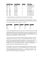
EPP2000 and ISA2000
Fiber Optic Spectrometer Manual
14390 Carlson Circle, Tampa, FL 34677
Phone 813-855-8687 fax 813-855-2279
email: [email protected]
web: www.StellarNet-Inc.com
-1-
CC Declaration of Conformity
According to EN45014
We
StellarNet, Inc.
Of
14390 Carlson Circle
Tampa, Florida 33626
USA
Declare under our sole responsibility that the products named below conforms to the following
standard(s) or other normative document(s):
Product name:
EPP/ISA Miniature Fiber Optic Spectrometers
Product type:
Analytical and Process Control Instrumentation
Product models:
Safety:
EPP2000, EPP2000C, EPP2000-HR, EPP2000-NIR-InGaAs,
ISA2000
EN61010-1, EN61010-2-031, IEC61010-3-1
EMC:
EN61326 + A1
Supplementary information:
The product complies with the requirements of the Low Voltage
Directive 73/23/EEC-93/68/EEC, and the EMC Directive
89/336/EEC-92/31/EEC & 93/68/EEC.
____________________
Will Pierce
President
November 11, 2003
StellarNet, Inc.
14390 Carlson Circle
Tampa, Florida 33626
-2-
Fiber Optic Spectrometer Manual
Introduction______________________________________________________
Quick Start Installation______________________________________________
EPP2000 Hardware Interface_________________________________________
Connector Interface Signals____________________________________
Special Interface Signals_______________________________________
Unit Address Selector_________________________________________
Power requirements___________________________________________
ISA2000 address and interrupt selector switches___________________________
SpectraWiz Software General Help_____________________________________
SpectraWiz File Menu _______________________________________________
SpectraWiz Setup Menu _____________________________________________
SpectraWiz View Menu ______________________________________________
SpectraWiz Applications Menu ________________________________________
3
5
7
8
9
9
9
10
11
15
17
22
26
Introduction
The EPP2000 (portable) and ISA2000 (plug-in) models are compact, fiber optic spectrometer
instruments, used to make various types of spectral measurements in the UV-VIS-NIR ranges.
When used for spectroscopy applications, the instrument can provide wavelength information
used to compute sample absorbance, transmittance, reflectance and emittance (used in
fluorescence and Raman spectroscopy). The unit can also be used to measure spectral
emissions from various light sources such as LED’s (Light Emitting Diodes), LASER diodes,
plasma furnaces, arc lamps, high and low pressure gases, and solar irradiation.
The units provide 2048 wavelengths for each scan over the factory configured range. The range
and coarse resolution are determined by the spectrometers installed grating groove density. The
fine resolution is determined by the installed slit size. The EPP2000 portables connect to a
computers digital parallel port using a standard 25 pin flat ribbon cable or IEEE 1284 rounded
cable. The ISA2000 plug-in is inserted into a computer’s ISA slot.
For multi-beam applications, up to eight EPP2000 units may be connected via USB-2 cables
AND up to eight ISA2000 cards may be inserted into a single industrial computer.
All spectrometer models have optical fiber signal input via female SMA 905 connector.
The list of spectrometer models is shown below (check our web site for the latest
configurations). The EPP2000C model has a special concave holographic aberration corrected
grating. This unit has no mirrors and therefore minimizes stray light and improves instrument
stability because there are less components in the optical plane.
The grating projects a flat field to provide a constant resolution and additionally provides
aberration correction for superb imaging. Another advantage over a ruled plane grating is
reduced surface roughness. This decreases grating scatter and improves detection limits. For
more information, download the white paper entitled “Introduction to reflective aberration
corrected holographic diffraction gratings”.
-3-
Model EPP or ISA
Wavelength range
Resolution
g/mm Grating
2000C-UV+VIS*
2000UV
2000UV2
2000UV3
2000VIS
2000NIR
2000NIR2
2000NIR2b
2000NIR3
2000NIR3b
2000NIR4
2000NIR4b
2000XNIR2
200-850nm
200-600nm
200-400nm
220-350nm
350-1150nm
500-1100nm
600-1000nm
785-1200nm
550-840nm
680-935nm
500-700nm
600-800nm
1200-1600nm
0.75nm
r1
r4
r5
r2
r2
r1
r1
r3
r3
r4
r4
r1
590, holographic-concave
1200, holographic-plane
2400, holographic-plane
3600, holographic-plane
600, ruled-plane
600, ruled-plane
1100, holographic-plane
1200, ruled-plane
1800, holographic-plane
1800, holographic-plane
2400, holographic-plane
2400, holographic-plane
1200, holographic-plane
* Not available in ISA2000. UV and XNIR2 models require UDET/XDET detector upgrade.
CUSTOM RANGES and Higher Resolution models AVAILABLE, contact factory for details.
Use the following resolution table only as a guide, actual resolution is much better. To figure
actual resolution, divide the range by number of detector pixels and multiply by blurr factor (2.5
for a 25um slit). Example: VIS = 800/2048 * 2.5 = 0.97nm
Slit size (microns)
r1-resolution
r2-resolution
r3-resolution
r4-resolution
10um
25um
50um
100um
200um
0.50
1.20
2.40
5.00
10.0
1.40
2.50
5.00
10.0
20.0
0.35
0.70
1.40
2.80
5.60
0.25
0.50
1.00
2.00
4.00
The slit is permanently installed in the fiber optic connector. It allows the instrument to maintain
resolution when different sizes of fiber optic cables are connected. If you plan to use only single
mode fibers 8um or smaller, then a slit is not needed. Most spectroscopy applications do
require a slit. Resolution indicates the instrument’s ability to resolve adjacent peaks at FWHM
(full width half max) separated by “resolution” wavelengths.
The current spectrometer models use 2048 element CCD (Charge Coupled Device) or PDA
(Photo Diode Array) detectors, or NIR 512 or 1024 element InGaAs detectors. Detector
specifications for your spectrometer model are available on our web site. Sensitivity for these
devices is extremely high and range from 100 to 200 V/(lx * s) as found in the detector
manufacturer’s specs (i.e.: Sony/ Toshiba/ Hamamatsu). The most common detector is an array
of 2048 cells of 14um x 200um tall elements each with a 14um pitch. The NIR InGaAs
detector pixels are 25um x 500um tall elements with a 25um pitch.
The SpectraWiz software provides for detector integration time selections down to 1ms (for
LT14 electronics) or 2ms (for LT12) or 4ms (for standard electronics). This is equivalent to
A2D (Analog to Digital) data acquisition rates of 2 / 1 / 0.5 MHz down (and slower). The
LT12 and standard A2D converter is 12 bit and therefore has a dynamic range of 1 to 4096
counts (+/- 0.5). LT14 is 14 bit with 1 to 16384 counts.
-4-
Quick Installation for SpectraWiz Software Summary
Installation for USB2EPP cable on Win98/ME/00/XP
1. If required, install adapter to add USB-2 ports. Cable will run 40x slower on USB-1 port.
>> Please note: software drivers should be installed before inserting adapter hardware.
Grab the driver CD from USB-2 adapter box and follow the manufacturers instructions. Note: for
Mercury brand adapters (VIA USB 2.0 drivers) run “setup.exe” on CD path =
"\USB\USB20_NEC\PC_Driver\setup.exe". OrangeUSB brand adapters under WinXP use
native Windows drivers, so insert adapter and Windows automatically installs drivers.
2. Insert USB2EPP cable with EPP2000 attached, into an available USB-2 port. When new
hardware found, insert the StellarNet CD or USB2EPP driver disk and provide path to the
appropriate folder “\SWDrivers-USB2EPP\Win2k” (for Win00/XP) or “\SWDriversUSB2EPP\Win9x” (for Win98/ME). On WinXP let windows to search for a suitable driver.
Installation for EPP-PCMCIA (by Quatech) or EPP-PCI (by Lava) card on Win9x/NT4
Install driver using documentation and diskette provided by card manufacturer found in adapter
box. Use Device Manager to verify new LPT port address (LPT2= 0278-027F or LPT3= 0268026F).
Installation for EPP-PCMCIA or EPP-PCI card on Win2000/XP
Install driver provided by StellarNet using the path to “\SWDrivers-EPP\Win2k”.
*** When installing the Lava PCI card, be sure to place it in PCI slot-0 or slot-1 ***
For integrated printer port (in EPP mode) use “Update Driver” in Device Manager.
When completed, use Device Manager to verify port address for the new WinRT device.
Install SpectraWiz from appropriate CD folder/disk (Win-9x-ME or Win-2k-NT-XP)
Win2000 only: after installation completes, goto SpectraWiz folder, click on Fix2000.bat.
Start SpectraWiz and verify spectral graph display. For parallel port operation, it is necessary to
Setup -> Interface port = Device Manager port address setting, and re-start.
After SpectraWiz installation, if irradiance calibration was ordered, install the cal files for
SpectroRadiometer operation using the StellarNet CD or diskette. The IRRAD-CAL files are
installed by clicking on the name “MyCal-nnnnn.exe” (nnnnn = spectrometer serial #).
If MyCal file was not supplied, then use Setup menu to install the wavelength calibration
coefficients listed on spectrometer label using “Setup -> Unit Calibration”.
Driver and software updates are easily downloaded from the StellarNet website
a. All drivers are in SWDriver
password=”wdriver”
b. SpectraWiz for Win95/98/ME password=”wiz”
c. SpectraWizNT for WinNT/00/XP
password="wiznt"
d. SWUpdate for all Windows vers
password= no password ßget the latest version now
Problems with Quatech EPP-PCMCIA card: Use Device Manager to select another IRQ.
Problems with Lava EPP-PCI card: In SpectraWiz folder, click on Lava2000.reg, then re-boot
after power off shut-down. This may require Plug & Play OS setting in BIOS => No.
For StellarNet technical support, Phone: 813-855-8687 or email: [email protected]
-5-
Installation for Win95/Win98/WinME
Non-Plug-and-Play Interfaces
The ISA2000 plug-in spectrometer and the EPP-ISA parallel port card from SIIG require
switches to be set for the port address and IRQ interrupt request selection, so you will first
need to find what is available in your computer using the Windows Device Manager.
Change the ISA interface switches to an available IRQ and port address by changing its
jumpers then install the card into your computer. Here are some helpful port addresses:
LPT1 378-37F hex IRQ7
LPT2 278-27F hex IRQ5 (default - can also be set to IRQ9, 10,11,12)
LPT3 268-26F hex IRQ9/ IRQ10/ IRQ11/ IRQ12
ISA2000 300-30F hex IRQ INTERRUPTS NOT USED (default all IRQ switches off)
(ISA2000 has switch settings for IRQ7, 9, 10,11,12,3,4,5)
See manual section on ISA2000 port address and interrupt selector switches.
For EPP2000, connect the IEEE1284 or ribbon cable, then plug-in the 5volt DC power.
If you intend to operate the EPP2000 from your desktop or notebook computer’s integrated
printer port, then goto step 2.
1. Install the SpectraWiz software for Win9x then start the SpectraWiz program. Using the
SpectraWiz Setup à Interface menu, configure the PORT address to be the same as found
using the Windows Device Manager settings. If you are using the PCMCIA card, you must
“uncheck” the box for LAVA PCI Card. Then press the button to update the registry and
restart SpectraWiz. The SpectraWiz Setup à Interface menu is normally displayed
automatically during the first installation. To access this menu later use the Setup à Interface
menu.
A real-time spectral graph should appear.
If not check the power and interface cable connections.
Also, try changing port address and IRQ.
2. To operate the EPP2000 from your desktop or notebook computer’s integrated printer port,
you must first configure the BIOS to enable the EPP mode on the printer port. Some
computers may not have this option, or may be faulty in operation. For these cases StellarNet
offers ISA bus, PCI bus, and PCMCIA card adapters that do work. These are low cost
IEEE1284 compatible high speed parallel port adapters.
Bring up the computers BIOS selection for integrated peripherals and select the parallel port
mode. Most computers provide BIOS selection only when the computer is first powered on by
pressing the “Del” key (or some other, possibly esoteric, combination of keys). Consult your
computer manufacturer to determine BIOS keystroke.
-6-
Using the BIOS menus provided, change the port mode to EPP or EPP+ECP. Please note the
mode cannot be set to the ECP only mode (or any other selection such as SPP, Bi-directional,
or Standard), as these will not work. If you cannot find an EPP mode selection, the EPP2000
will not work. An EPP-PCI or EPP-PCMCIA card is needed.
Using the BIOS menu, verify the LPT port address (normally 378 hex). Later, set the
SpectraWiz Setup => Interface port configuration to the same port address.
After setting up your BIOS and verifying the Port and IRQ settings using the Windows Device
Manager Goto step 1.
DOS SpectraWiz
If you are operating under Win9x/ME it is a good idea to verify the adapter port installation
using Windows Device Manager. Please note that an IRQ assignment is required. Next open
a Dos window and continue as follows:
Insert the SpectraWiz (Dos) diskette and run a:INSTALL.BAT. This creates a directory on
your hard drive named C:\SW and copies all files into it.
Change directory into c:\SW (“CD \SW”) then type the command SWZ. This will start the
SWZ.BAT file. It performs the basic setup required for operation on LPT2: then runs the
SW.EXE. To use a port that is configured for LPT1 (378 hex IRQ7), execute the SW1.BAT
file instead.
If you are running Windows you may wish to create a shortcut to the SWZ.BAT
file using the Windows Explorer and place it on your desktop. For proper
SpectraWiz operation, the Memory properties should be all set to Auto. The
Conventional memory Protected option should be enabled. Both EMS and
XMS set to Auto and Uses HMA should be checked(enabled). Under Misc
properties-> Foreground -> Allow screen saver set unchecked(disabled).
EPP2000 Hardware Interface
The DB25 connector on the rear panel of the EPP2000 communicates with the connected
computer using the IEEE 1284 protocol for Enhanced Parallel Ports (EPP). Since the unit
provides over 2000 wavelengths for a single scan request, we called it the EPP2000. The IEEE
1284 interface specification is really a hardware handshake mechanism that allows high-speed
data transfer into and out of the computer.
Older PC’s did not support the bi-directional EPP transfer mode on the printer port. Most of
the newer PC’s (after 1995) do support this mode, however there are always a few exceptions.
Even though the IEEE1284 standard is published, there are a few PC’s that don’t work just
right (even thought they say they do). They may only support the ECP mode but not the EPP
-7-
mode (The ECP mode is the Enhanced Capabilities Port mode and is the “Cadillac” mode) or
it just doesn’t work perfectly like it should.
We recommend using the new USB2EPP cable for best performance via USB-2 ports.
Otherwise a second parallel port should be installed for the EPP2000 spectrometer(s). These
are the EPP-PCI for desktops or EPP-PCMCIA for notebooks. This ensures 2 things: 1) the
spectrometers will always work immediately with this low cost adapter card and no time will be
wasted on installation and testing. 2) You will be able to printout the spectra at almost at the
same instant that you display it using the systems LPT1 printer.
When you are using a notebook computer with the EPP2000 spectrometer, it is possible to
connect the instrument directly to the printer port. For some notebooks this may not work,
however an alternative exists to provide the desired result. A PCMCIA adapter is available to
provide a second printer port that is EPP capable and compatible with the EPP2000
spectrometer(s).
The EPP architecture and signaling protocols provide a mechanism for a fully interlocked data
transfer within a single CPU I/O cycle. What this means is that when an I/O instruction is
executed, the port hardware will synchronize with the external peripheral (EPP2000
spectrometer) and automatically generate the necessary handshake signals to transfer data to the
peripheral or receive data from the peripheral. This provides transfer data rates to over 2M
bytes per second. This translates to over 1 million wavelengths per second !
EPP2000 Connector Interface Signals
The DB25 connector contains standard parallel port signals plus a few that have been defined in
EPP mode for the EPP2000 spectrometer, which is allowed by the IEEE1284 specification.
The SPP signals identified in the table below show the Standard Parallel Port signals as
originally defined on the IBM PC 25 pin printer connector. The I/O (input/output) column
below is from the computer’s point of view, with exception to the user-defined signals. All
signal are 0 to 5 volts DC (TTL).
Pin
SPP Signal
EPP Signal
1
14
17
16
10
11
12
13
15
2-9
nSTROBE
nWRITE
nAUTOFEED
nDATASTB
nSELECTIN
NADDRSTB
nINIT
nRESET O
nACK
nINTR
BUSY
nWAIT
PE
user defined
SELECT user defined
I
nERROR
user defined
Data 0-7
Address 0-7
I/O
EPP Signal Description______________________
O
Active low, indicates a write operation, high on read
O
Active low, indicates Data read/write operation
O
Active low, indicates Address read/write operation
Active low, peripheral reset command.
I
Peripheral interrupt to the host computer.
I
Handshake. When low OK to start a strobe cycle.
O
Low to High indicates start of spectral scan (TTL)
Spectrometer auxiliary power bus +5Volt input
I
External trigger, hold low to disable (TTL)
BI
Bi-directional Address/Data lines.
-8-
EPP2000 Special Interface Signals
The above DB25 computer interface connector contains user defined signals specific for the
EPP2000 spectrometer on pin 12, 13, and 15. Any of these signals can be mounted to rear
panel jacks via special request.
Pin 12 is an EPP2000 spectrometer output to indicate start of scan. This may be tied to a
XENON strobe lamp’s trigger input to flash the lamp at the beginning of each scan.
Pin 13 is used to supply power to the EPP2000 spectrometer when the USB2EPP cable is
used or multiple units are connected on the same ribbon cable. Note that the power supply
must be capable of providing the appropriate current for the number of units connected. Each
standard unit requires 250ma of current at +5VDC. We recommend that a power adapter be
used with the USB2EPP cable for best performance. LT12 and LT14 spectrometer electronics
require just 100ma, however spectrometers with an integrated TE temperature regulator, such
as LT14 NIR-InGaAs spectrometers, require 1300ma.
Pin 15 is used as a syncronizing input to the EPP2000 spectrometer. It provides a hardware
scan enable when high (and scan disable when low). TTL switching delay is less than 1 microsecond.
EPP2000 Unit Address Selector
For multi-channel applications, multiple units may be connected to the same parallel ribbon
cable using different unit address selections. However, if the USB2EPP cable (Universal
Serial Bus USB-2 ) is used, all EPP2000 spectrometers are set to the same unit address of 1.
Parallel cables with extra DB25 male connectors are available or can be easily fabricated. Up
to 8 units can be connected in this way. Each unit has a unit selector dial that can be set to the
desired unit address. The instrument may be addressed as unit 1-8 through a small pinhole
adjacent to the DB25 female connector on the rear panel. The factory default selection is unit
1. The selector switch is a rotary dial that has a vertical slot when unit 1 is selected. Using a
jeweler’s screwdriver turning clockwise 1 click will select unit 2 (then unit 3 and so on).
EPP2000 Power Requirements
A standard EPP2000 spectrometer requires a 220-250ma (milliamps) at +5VDC. The power
supply must be regulated. A single unit may be powered by a 300ma +5VDC wall transformer
with 5% regulation. Up to 4 units can be powered by a 1 amp +5VDC wall transformer with
3% regulation. The input power on the EPP2000 is a 2.5mm male power jack (the wall
transformer must have a 2.5mm female connector).
LT12 (Little Turbo 12-bit) and LT14 (Little turbo 14-bit) spectrometers require only 100ma.
Look for the LT12 or LT14 identification on the bottom label.
-9-
An optional Battery Power unit (BP1) is available for the EPP2000. It contains a 2.4 amp
hour rating which will power the spectrometer for about 8 hours. The BP1 includes a +12VDC
wall transformer to re-charge the battery.
ISA2000 Hardware Switch Selections
The base address for the spectrometer plug-in card is selected with 4 slide switches at location
U68 (just above U43). The board may be place at 16 different locations from 300 hex – 3F0
hex. using the following address switch configurations. The default factory address for single
board applications is 300 hex.
300 hex = X X X X all switches are up (X = on position)
| | | |
1 2 3 4
ßswitch position marking
310 hex = | X X X
X | | |
320 hex = X | X X
| X | |
330 hex = | | X X
X X | |
340 hex = X X | X
| | X |
350 hex = | X | X
X | X |
360 hex = X | | X
| X X |
370 hex = | | | X
X X X |
380 hex = X X X |
.
| | | X
7 additional address locations for 390 hex-3F0 hex can be
configured using switches 1-3 with switch 4 down.
The interrupt selection is made by setting only one switch (of 8) at location U69 in the UP
(on) position. The interrupt request lines (IRQs) available are as follows. The default IRQ
address for single board applications is IRQ 7.
6
7
8 ßswitch position marking
1
2
3
4
5
3
4
5
7
9 10 11 12 ßIRQ selection
- 10 -
SpectraWiz Software General Help
////////////////////////////////////////////////////////////////
Experiment Procedures.."how to get started taking data"
ToolBar Icons..........areas on the screen for mouse operation
System Indicators......show you what's on/off at a glance
////////////////////////////////////////////////////////////////
Experiment Procedures //////////////////////////////////////////
Ensure that you have installed the calibration coefficients for
your unit. Use the Setup->Unit calibration coefficients menu
to enter the 3 coefficient values found on the spectrometer
label. This information tells the software how to provide the
wavelength readouts. For a single unit EPP2000 spectrometers,
select unit 1 with physical address 1.
If you are interested in emmission applications, ie: looking
at light sources, LEDS, laser diodes, plasma, or even fluorescence, then you can start observing right away in the "Scope
mode" which is the default view mode at start-up. Otherwise,
for applications requiring spectroscopy modes such as Absorbance or Transmission or Reflectance (same as Transmission),
selecting the proper "View mode" after taking a Dark and Reference scan is simple enough. Note the "Dark bulb" and the
"Light bulb" icons on the toolbar for this.
Taking a Dark scan for the Scope mode becomes important with
detector integration times well above 250ms (above 1/4 second).
Although it is not required, doing so will eliminate detector
structure baseline, which is a pixel non-uniformity constant.
Always take a "new dark" after changing system parameters such
as samples to averaging, smoothing, and detector integration.
To take a dark scan, you must block the light signal input to
the spectrometer or turn off the light for a moment.
There is an alternative approach to taking the Dark scan. This
makes it a bit easier because you don't have to block the input
signal. Instead of using the left mouse click on the Dark light
bulb icon, use a right click to "zero the Dark". Now, ensure
that the Temperature compensation selection in the setup menu
is turned on (enabled). This feature evaluates the dark level
in the "optical black" region of the detector and removes this
level from the input signal on an ongoing basis. This bit of
magic eliminate the need for a dark level shutter.
In all modes, X zooming and Y re-scaling allow regions of
interest to be easily viewed. Remember, X zooming allows
exclusion of areas that may cause auto Y re-scaling to fail
because of large peaks on left or right. A little "hands on"
allows simple navigation with the tool bar.
Before "viewing" Absorbance or Transmittance we must first
setup some basic system parameters and save a "dark" and "reference" scan. This is performed in the default "Scope" view
mode.
1. Setup and turn on your reference light source so that you
are now viewing a bell shape curve in Scope mode. For
- 11 -
reflectance, using a fiber probe, hold at 45 deg to your
white standard about 1/4 inch away. For cuvette holders,
use cuvette in place with no sample. For dip probes,
use your solvent solution for reference.
The curve MUST NOT touch the top of the graph. If the
slider bar on the toolbar is already max (for fastest
detector integration rate), then you must reduce the
input signal by using a smaller fiber or insert a filter.
For reflectance, just move the tip back from the white
standard (reference) surface. For others, you may test
this out by backing out the SMA 905 fiber optic connector
from either the light source or spectrometer.
2. We recommend you start with (and setup) the following
configuration until you are familiar with the options.
Use the Setup menu:
Detector integration rate
Number of Scans to average
Pixel resolution (smoothing)
Temperature Compensation
=
=
=
=
50 millisec
5 (if below 100 ms)
0 (NONE)
1 (ON)
Note: if the first 3 items are changed, then you
MUST AGAIN save a new "dark" and "reference" scan.
3. Adjust the detector integration until the bell curve
fills 90 percent of the graph. The longer that the
detector integrates, the larger the input signal.
Perform a File ->Save-> Reference from the menus or
click the yellow light bulb icon on the toolbar.
4. Now block the light at your light source. If you
can't then you will have to turn it off for a moment.
Perform a File ->Save ->Dark or click the dark light
bulb on the toolbar.
5. At this point you are ready to view Absorbance or
Transmission using the View menu selection.
Absorbance and Transmission should appear as flat
lines. Insert your sample and observe the response
in realtime. You may now save to disk or print the
sample graph.
////////////////////////////////////////////////////////////////
ToolBar Icons //////////////////////////////////////////////////
Move Data Cursor [picture of graph with arrow left/right]
left <"After" placing the data cursor by pointing
right ->
and clicking the right button, each
subsequent click here (using the left button)
will move 1 pixel in direction selected.
To remove data cursor click to left of graph.
>>> Clicking the right button on these icons
will seek to the next peak in the selected
direction, and place the data cursor there.
File save
[picture of diskette]
- 12 -
sample
Same as menu File->Save->Sample (to disk)
Save dark
spectrum
[picture of DARK light bulb]
Used for Absorbance, Transmittance, and
Irradiance modes.
Left Click here with light off.
Caution: Right Click will zero previous dark.
Save reference
spectrum
[picture of YELLOW light bulb]
Used for Absorbance and Transmittance modes.
Left Click here with light on and
without sample in place.
When viewing Irradiance -> watts per square
meter, clicking here starts the UV monitor
application.
Print graph
[picture of printer with white paper]
Left Click to plot graph on printer.
Snapshot spectra [picture of camera]
Left Click here to freeze graph trace.
Left Click here again to unfreeze!
Zoom wavelength
[picture of Z]
Reminds you how to X and Y Zoom.
Left Click here again to UN-Zoom! Also,
Left Click on left side of graph to UN-Zoom.
Right Click to enable Y zoom mode.
Re-scale Y axis
[picture of graph with up+down arrows]
Left Click here to AUTOSCALE Y axis.
Right Click to UNDO AUTOSCALE Y axis.
Also use View->Y set scale menu to
override AUTOSCALE with selected scale.
Compute Area
[picture of peak area with green]
Left Click here to show the AreaPSD,
Centroid, Peakwave, FWHM, and Centbase
of a peak. If the data cursor is
not on a peak, the icon will seek to a
peak in the closest direction.
Right Click to start dual data cursor
measurement as outlined below.
This information is printed in the graph
title (concatenated to end of line) when
printing a graph.
Compute Area toolbar function details
------------------------------------1. Use left mouse click to compute and display:
AreaPSD, Centroid, Peakwave, FWHM, and Centbase
>> Automatically selects closest peak & finds baseline.
>> AreaPSD = integral Area (Power Spectral Density).
>> Centroid = center wavelength of AreaPSD in nm.
>> Peakwave = wavelength of the tallest point.
>> FWHM
= Full Width Half Max of peak in nm.
- 13 -
>> Centbase = level used to compute AreaPSD & Centroid.
2. Use right click to start dual cursor measurement for:
AreaPSD, Width, Base (via user positioned cursors)
a. Position data cursor to right of area to measure,
using right click on graph at desired location.
b. Then right click Area toolbar icon and this will
change the data cursor to a dashed line.
c. Now position a second data cursor to left of area
at desired location on graph with right click.
d. Right click Area toolbar icon to display the
AreaPSD, Width, and Base measurements.
e. Right click Area toolbar icon to resume with
normal data cursor as a solid line.
Key words on horizontal menu:
Sco
Abs
Tran
Irad
Click on these words to quickly switch modes.
Equivalent to selecting the View menu options:
View
View
View
View
->
->
->
->
Scope mode
Absorbance
Transmission
Irradiant Watts
=
=
=
=
Sco
Abs
Tran (also used for reflectance)
Irad
////////////////////////////////////////////////////////////////
System Indicators ///////////////////////////////////////////////
Observe the system indicators appearing below the graph in the
status panel.
SCOPE-> Wave:534.6nm Pix:1050 Val:138.600 Time:4ms Avg:5
(normally single line) Smooth:0 Tc:off Z Y
Z
Y
y
Tc
means that you have performed an x-axis zoom
means that you have performed a Y rescale or Y zoom
means that you have enabled the Y zoom mode
Temperature compensation on/off
Smooth
Pixel smoothing 0=none
1=5 pixel
2=9 pixel
3=17 pixel
4=33 pixel
Number of samples averaged
Detector integration period in milli-seconds
Magnitude at the data cursor
Location of the data cursor (0-2050 pixels)
Wavelength at the data cursor location
Currently selected mode (also TRANS/ABSOR/REFS/IRRAD)
Avg
Time
Val
Pix
Wave
SCOPE->
////////////////////////////////////////////////////////////////
- 14 -
SpectraWiz File Menu
//////////////////////////////////////////////////////////////////
Save...................current spectra sample data to disk file
Open...................spectra file for graph display & print
Print Setup............allows page layout selections for graph
Print..................current graph sample data to print device
Exit...................terminate SpectraWiz program
//////////////////////////////////////////////////////////////////
File -> Save:
Allows the user to save spectral data to files.
Options are Sample, Reference, Dark, and Export.
Access via File->Save menu, disk icon, or Alt+Disk menu
File->Save->Sample: (icon with arrow to diskette)
In Scope mode -> Sample saves filename.SSM files
Trans mode -> Sample saves filename.TRM files
Absor mode -> sample saves filename.ABS files
Irrad mode -> sample saves filename.IRR files
The Sample files are text and can be read into a spreadsheet program such as Excel using the "delimited" option
using the "space" delimiter. The output format is
wavelength(x-axis) <spaces> value(y-axis) <new line>
The File->Save->Sample dialog allows the user to select
the filename to create. This dialog has a "Save as type"
pull down selection. Using this feature you can save
the file as a Galactic Industries - Grams/32 SPC file.
These files can be dragged from the Windows Explorer
"SpectraWiz" directory onto the Grams/32 graph program
with the click of your mouse!
File->Save->Reference: (icon with yellow light bulb)
File->Save->Dark:
(icon with dark light bulb)
The Reference file "SW.REF" and Dark file "SW.DRK" are
saved when setting up an experiment that requires the
Absorbance or Transmission modes.
The save icons on the toolbar perform
the same functions for above features very quickly.
Refer to General Help for more detail on this.
The File->Save->Export selection allow the user to
setup the "starting","increment", and "ending" wave
lengths. This feature linearizes the output data.
This allows output wavelengths to be evenly spaced,
and can be enabled or disabled. When disabled the
wavelength for each detector pixel is output. The
wavelengths will not be evenly spaced due to the
dispersion of the spectrograph.
Using Alt+D to save to disk (or clicking on the
horizontal menu item "Disk") you can use the auto
filename increment feature. Each time you specify
a basic filename, subsequent saves will append a
number to the name, saving you lots of time !
- 15 -
When multiple channels are enabled, a file ->
save -> sample -> automatically saves all channels.
This occurs ONLY when the VIEW -> Multi-Graphs has
first been enabled. Each channel will then append
its channel number. For example if the file name
to save is given as TEST and you are in absorbance
view, then the files for a 3 channels configuration
will be saved as Test1.abs, Test2.abs, and Test3.abs.
//////////////////////////////////////////////////////////////////
File -> Open:
Allows the user to select various files to be read back in
which were previously stored using the Save function.
The graph may be zoomed or printed. The system is placed
in the "SNAP" mode. To return to normal operation click on
the camera icon (which turns SNAP off).
Open allows multiple spectral traces to be graphed. To
select multiple files to graph, press and hold the Ctrl key
while highlighting the file names to be graphed. This is
a standard way of selecting multiple files in Windows.
Each spectral trace is graphed in a different color.
Trace colors can be configured via Setup => Channel Display.
Select the .ep file type to view an Episodic data capture.
This will display a series of spectral traces in 3d from
the file that was created using the Setup => Episodic data
capture feature. Alternately, you may select specific
wavelengths to be extracted and graphed as time series.
The time series data can then be saved to file as .ts file
types - one at a time. Each file will represent action for
a selected wavelength over the episodes time. The .ts files
can be opened and graphed in multiple. It is suggested that
these files are named appropriately when saved. The .ts file
types can be imported into Excel because they are in text
using space delimited format for timesamp and value.
//////////////////////////////////////////////////////////////////
File -> Print:
Allows the user to plot the currently selected screen on
the connected printer device. A graph title is optional
and will print with date.
Graph print information can be optionally configured using
the Setup menu. Up to 4 items can be requested from the
operator each time the print option is selected. This
information will be printed as the graph title line. It
is primarily used for QC of samples, where the information
might include serial or batch number, temperature, etc.
//////////////////////////////////////////////////////////////////
- 16 -
SpectraWiz Setup Menu
///////////////////////////////////////////////////////////////////
Detector integration time....sets new detector integration period
Number of scans to average...Y axis smoothing improving sig2noise
Spectral smoothing controls..X axis smoothing improving sig2noise
Temperature compensation.....periodic baseline shift compensation
XTiming resolution control...selects modes for Standard/Extended
Episodic Data capture........collect spectral data over time
Optical Trigger..............select wavelength and trigger level
Spectrometer channel.........enable drift correct or map
Actions for peak icon........auto find and continuous mode
Display Refresh rate.........and Slide bar range settings
Channel display trace........color selections
Graph Print Info Prompts.....allows customization of title line
Interface Port and detector..Hardware setup for instrument
Unit cal coeficients.........setup for wavelength readout
Warning message Enable.......disable/enable new dark save needed
///////////////////////////////////////////////////////////////////
Detector integration time
This should be adjusted for each experiment to maximize
the detector output and signal to noise ratio. The
integration time is reported in the status bar message
below the graph (as Time: xx milli-seconds). The toolbar
slidebar can be used to dynamically set the appropriate
level without saturating at the graph top.
Units configured as "non-XTiming" (special order), require
time selection in terms of Kilo Hertz (instead of milli
seconds), which relates to the Analog to Digital converter
conversion time in cycles per second (KHz).
//////////////////////////////////////////////////////////////////
Number of scans to average: 1..999
Sets the number of spectra to signal average. Please note that
the real-time display is updated AFTER this number of spectra
have been aquired. This option provides a smoothing in the Y
axis, effectively increasing the system signal to noise by the
square root of the number of scans being averaged. Set the
scan averaging to the highest number tolerable when there is
plenty of light signal and the detector integration time is
short. Even when you have a moderate level of signal, it is
best to wait a few seconds to improve the measurement quality.
//////////////////////////////////////////////////////////////////
Spectral smoothing controls: 0=>disable
Pixel Boxcar smoothing level 0..4 => 0/5/9/17/33
This performs data smoothing by applying a moving average of
adjacent pixels to the data arrays. For example, 1 would
average each 5 pixels with the 2 pixels on the left & right.
0 performs NO data smoothing. Smoothing levels 1..4
correspond to the input fiber image size for 50,100,200 & 400
micron diameter fibers respectively.
Savitzky Golay level 0..4 => 0/9/13/17/21 point smoothing
- 17 -
Spectral smoothing algorithm that avoids crushing peaks.
published in Analytical Chemistry - July 1964.
First
Display Persistance level 0..9
This controls smoothing for digital readout displays using
exponentially smoothed averaging. For example, spectral data
is used to compute the ChemWiz concentration for selected methods.
Average dark baseline: checked=ON
This controls the baseline average level to keep it above
zero. The algorithm computes the average dark level and makes
the average the zero baseline. Using long detector integration
times will move this level higher using "Scope mode". When
measuring fluorescence it may be desirable set this feature
off so the baseline is maintained at a real zero level.
//////////////////////////////////////////////////////////////////
Temperature compensation: checked=ON
The first 30 "optical black" pixels that are read from the
detector provide a useful level of the sensor dark current
even when the detector is illuminated. If this option is on,
the system periodically samples this area and makes an
adjustment to the normal readout. When the level raises
or lowers with temperature the scan is adjusted accordingly.
//////////////////////////////////////////////////////////////////
XTiming resolution control: 1/2/3
This feature provides increased optical resolutions.
Selection 1 is the lowest optical resolution and
is syncronized with the selected detector integration. In
general, if your requirements for optical resolution are
greater than 1nm, then selection 1 is ok.
Selection 2 or 3 slow the digitizer & detector clock
by a factor of 2/4 respectively. With XT levels 2 & 3 you
will be able to observe increasingly higher resolutions.
The detectors signal amplifier improves with slower thruput.
When selecting XT level 2/3 the detector integration time
must be increased to 30ms or longer to avoid sync delays.
//////////////////////////////////////////////////////////////////
Episodic Data capture:
Saves spectral data over time. Allows a specific number of
episodes to be saved or can be continuous with the operator
signaling when to stop by clicking on the dark light bulb.
A time delay can be inserted between each capture. The data
can be graphed in 3d using the File -> Open function and
selecting the .ep file type. When the user specifies the file
name such as "test", then a file test.ep1 will be created. If
there are additional channels active (up to 8), additional files
will be created such as test.ep2 (up to test.ep8). Each file
contains an internal time stamp with milli-second resolution.
The .ep files are not in text format, however the data can
be extracted into text form as a time series. Use File -> Open
to perfrom the extraction of a selected wavelength over time, then
save it as a time series (.ts) file type.
- 18 -
Episodic data capture can be combined with the optical trigger
function. First setup the trigger to operate in continuous mode
at the desired wavelength and trigger level as a percent of
scale, then start the Episodic data capture. The system will
capture events pre-qualified by the trigger level. You can
select a specific number of events to record or allow it to
record until terminated by the operator.
//////////////////////////////////////////////////////////////////
Optical trigger parameters:
Setup optical trigger level at a specified wavelength in
terms of absolute value or percent of scale by using the
percent symbol %. If you enter 75% as the trigger
level, then when an external event occurs, the wavelength
prescribed must reach at least 75% of the scale setting. If
you are in SCOPE mode with 4096 as the upper scaling, then
the wavelength maginitude must reach 3072 for the system
to display the event.
Setting the wavelength to zero (0) turns the trigger function
off. Also, setting the wavelength to one (1) allows ALL
wavelengths to be monitored for event trigger level.
Once an event has triggered, the display trace
will NOT update until a new trigger has qualified. You may
select SNAP to permanantly trap the spectra. This action
turns off the trigger. The spectra may now be saved to file
or printed.
The optical trigger can be used in conjunction with the
episodic data capture feature. This is a powerful data
collection tool. Additionally, when multiple channels are
enabled, each channel can be selected to have its own
wavelength and trigger level.
//////////////////////////////////////////////////////////////////
Spectrometer channel enable:
Drift correct reference:
Enter the single channel reference wavelength, or enter
channel number (1-8 for multi-channel configurations).
The single channel options are "Delta" from a baseline or
"Absolute" as a zero. The wavelength selected is used to
stabilize the absorption / transmission / reflectance
measurements for single channel spectrometers. The
wavelength is carefully chosen to not have any absorption
from the sample, effectively providing a reference beam
from the light source. Any fluctuation in the light source
or sample due to temperature or otherwise will be removed.
If you have a second channel that has a similar wavelength
range, it can be setup to monitor the lamp drift. Enter
the channel number to enable dirft correct. If there are
additional computational channels, each will be corrected
by the channel you select. This assumes the other channels
use the same light source.
- 19 -
Map Logical to physical:
If you have multiple spectrometers this provides a setup.
This allows setup of the LU (Logical Unit) to physical unit
address. A similar input is made under the Setup->Unit
menu, however this selection does not deal with the coefficients. A cross check is also made to determine if multiple
LU's have the same physical address. Each system must have
at least 1 but only 1 unit at physical address 1.
The system can handle LU's 1-8 with physical addresses 1-8.
On the EPP2000 the physical address is set by turning the
rotary dial on the back panel using a jewelers screwdriver.
//////////////////////////////////////////////////////////////////
Actions for peak area icon:
Auto Find Peak:
Cursor attempts to locate peak, otherwise operation uses
current location of the green data cursor.
Continuous mode:
Allows continuous update after clicking peak area icon.
Action terminates when icon is clicked again.
//////////////////////////////////////////////////////////////////
Display Refresh rate:
If you don't like the default setup of 250 milli-seconds,
then change it! We did not want to keep the Windows computer
too busy! The faster the machine, the faster you can go!
This option actually controls how fast the computer does a
scan request to the spectrometer. The data is aquired, then
processed and displayed. The system is prevented from requesting another scan until the current is finished.
//////////////////////////////////////////////////////////////////
Channel Display Colors:
Allows the default trace colors to be altered. Daahhh!
//////////////////////////////////////////////////////////////////
Graph Print Info Prompts:
This powerfull feature allows customization of the graph title
line that is printed. The user is prompted for up to 4 pieces
of information when the graph is printed. Each prompt may be
specified in this setup. Each piece of information is concatenated into a single title line along with its short hand
prefix label which is also specified in this setup.
//////////////////////////////////////////////////////////////////
Interface Port and Detector:
During installation, you may have found conflicts in your
Windows computer configuration. SpectraWiz automatically
uses this menu when hardware problems are found.
One can determine the available Port address by
using the Windows control panel under computer resources.
Your hardware interface adapter should be set to an available
Port address using physical jumpers on the cards.
- 20 -
Use this option to tell the SpectraWiz software where the
new hardware interface has been set. Once the new port has
been selected from the menu the Windows registry is updated.
An option box for the LAVA PCI adapter appears on this panel
(EPP-PCI card). Check the LAVA box if this is the interface
that you have installed (and NOT if your using the Quatech
SPP-100 (EPP-PCMCIA card) or the computers integrated
printer port). Under Win9x these cards need a port address
matching the device managers port resource. This is
not required for Win2000 or WinXP because port selection
is provided by the driver.
For USB operation with the StellarNet USB2EPP cable,
the port address is not used.
//////////////////////////////////////////////////////////////////
Unit calibration coefficient:
This allows the setting of the wavelength calibration coefficients for the spectrometer(s) in use. In addition the
user selects the physical unit address for each LU (Logical
Unit) handled by the display graph. For multiple unit
applications this allows simple configuration.
Pressing enter will make no changes.
The coefficients are
determined from a least squares fit to a second order polynomial which can be performed by any spreadsheet program
if you have a set of data points.
Using a wavelength standard such as a low pressure mercury
argon lamp, known emission lines can be read at various
pixel locations and used for calibration as described above.
The first, second, and third co-efficients are taken from the
calibration label attached on each unit and may be input
exactly as read at the c1, c2, and c3 software prompts.
If the calibration is NOT installed the wavelength X axis
will not be set correctly and the data cursor wavelength
readout will be incorrect.
//////////////////////////////////////////////////////////////////
Warning message Enable: checked=enabled
Allows user to disable/enable the message that indicates tha a
new dark save is needed. This occurs when new detector integration rates, samples to average, or pixel smoothing is
changed by the user.
//////////////////////////////////////////////////////////////////
- 21 -
SpectraWiz View Menu
//////////////////////////////////////////////////////////////////
Scope mode.............displays uncompensated spectral data
Absorbance mode........display requires dark & reference for AU
Transmission mode......display requires dark & reference for %T
also used for reflectance measurements
Irradiance mode........display Watts,Micro-Watts,Lumens,Moles,fc
Ref spectra............display of reference spectra minus dark
Channel................display selection for logical units
Multi-Graphs...........display channels in multi-windows
SnapShot...............freeze display or run in realtime
Wave Ratio.............select 2 wavelengths for ratio display
Y scale................setup max Y-axis or set Y to log scale
Zoom...................X and Y axis area you want to see
Graph Trace as.........Overlay or 1st or 2nd Derivative
//////////////////////////////////////////////////////////////////
View -> Scope mode:
Allows user to view spectrometer information in realtime.
Typically, this will be light emission from samples in
various forms for specific wavelength measurement applications
which include emission, fluorescence, and Raman (laser
induced scattering).
Scope enables viewing emission from LEDs, laser diodes, flourescent lamps, plasma, ignited metal or gas emission lines,
emission lines from the stars when mounted in a telescope,
light bulbs (all types), neon and other types of signs,
UV or laser induced fluorescence from samples, and Raman
scattering from samples.
Each pixel is graphed on the x_axis as wavelength in nanometers using the calibration parameters entered via setup.
Scope view will be affected by options available in
the Setup menu including; detector integration rate (spectra
signal level), number of scans to average (Y axis smoothing),
pixel resolution (X axis smoothing), Temperature compensation
(pulls dark spectra level to near zero over operating
temperature range).
//////////////////////////////////////////////////////////////////
View -> Absorbance:
Displays absorbance at pixel n using the current sample,
reference, and dark data sets:
A(n)=-log((sample(n)-dark(n))/(ref(n)-dark(n)))
//////////////////////////////////////////////////////////////////
View -> Transmission: (also use for Reflectance)
Displays percent transmission at pixel n using the current
sample, reference and dark data sets:
T(n)=((sample(n)-dark(n))/(ref(n)-dark(n))*100
Percent transmission is mathamatically eqivalent to percent
- 22 -
reflection and is used for reflectance applications.
Use transmission mode for SpectroColorimetry. Use a white
light to reflect off of a white surface. Save this as the
reference. Then replace the white standard with a color
sample to measure. You will then see the spectral shape
for the color where the white standard displays as a
straight line at 100 percent.
//////////////////////////////////////////////////////////////////
View -> Irradiance:
Watts per square meter (per nanometer)
Micro-Watts per square centimeter (per nanometer)
Micro-moles per square meter per second (per nanometer)
Lumen per square meter LUX (illuminance)
Lumen per square foot FC (footcandles)
These spectroradiometer display modes provide a calibrated Y
axis. In order to use this mode, the unit requires certain
system calibration files to exist. Units ordered as a
spectroradiometer include calibration files for operation
in this display mode. These files are installed by clicking
on the MyCal-nnnnn.exe file provided in the installation disk.
To get moles, watts is multiplied by 0.00835 (an Einstein),
which is a unit of energy in photochemistry, that represents
a Dose of power that irradiates a sample for 1 second. An
Einstein is the amount of enery in 1 mole (Avogadro's number,
6.0222 x 10^23) of photons. Another number displayed in this
mode is PAR, which stands for Photosynthetically Active
Radiation, and is the integral of power from 400-700nm in
micro-moles per square meter per second.
For the illuminace display, the photopic response curve is used
to formulate lumen per meter^2 which provides a LUX value.
The Irradiance calibration function located under the Apps
menu can re-generate system calibration files needed for
operating in Irradiance view mode. This requires a calibrated
source lamp with its calibration data stored in a disk file.
An example irrad cal data (text file) "NIST.icd" is
provided. This file can be used to simulate an irradiance
calibration and produce the required system calibration
files needed for selectiong the Irradiance view mode.
WARNING: the system irradiance cal files files such as
SW1.icf thru SW8.icf can be easily overwritten.
Like most instruments, it is good practice to re-calibrate
the spectroradiometer every 6 months.
Setup for Radiant
CR1............
IC2............
Other..........
Reset 1 sqm ...
and Luminous Flux Area in sq meter:
11 mm diameter -> sq meter
0.625 inch diameter -> sq meter
user defined
default area = 1 square meter
Radiant flux in watts = irradiance * surface area
Luminous Flux in lumen = illuminance * surface area
- 23 -
Setup range for watt and Rflux measurements:
Specify the start and end wavelengths for the range
computation of the total power. The default range
is 400-700nm.
//////////////////////////////////////////////////////////////////
View -> Ref spectra:
Displays the reference and dark data previously saved as
ref(n)-dark(n). This is useful for troubleshooting absorbance
or transmission applications. The Ref spectra must not be
clipped at its peaks, indicating a bad reference.
//////////////////////////////////////////////////////////////////
View -> Channel:
Allows display selection for logical units when more than
1 spectrometer is installed. If you have multiple spectrometers this selection allows you to view data from the different optical channels. Note: use "Setup -> Spectrometer
channels" to map different physical channels into the logical
unit selections (1-8).
//////////////////////////////////////////////////////////////////
View -> Multi-Graphs:
Allows display of multiple channels in a single graph.
Re-select to turn this feature off. The x-axis labeling can
be switched by using view -> channel -> n. All active
channels will be displayed.
//////////////////////////////////////////////////////////////////
View -> SnapShot:
Allows user to freeze display. Re-selecting SnapShot when the
display is frozen will re-start normal realtime display.
//////////////////////////////////////////////////////////////////
View -> Wave Ratio:
Allows 2 wavelengths to be selected to be displayed as a
ratio in the upper left hand corner. The default values
260/280 are used for DNA concentration measurement.
//////////////////////////////////////////////////////////////////
View -> Y scale:
Set Max Y:
Allows the user to specify the Y axis scale top value.
Selecting Y-axis rescale icon (left click) will override
the Max Y via autoscale. Entering a value of 0 will also
perform an autoscale.
as Log:
Converts the Y-axis into a Log base10 scale. Re-selecting
will convert back to a linear Y-axis.
- 24 -
//////////////////////////////////////////////////////////////////
View -> Zoom: ON/OFF
Allows a selected region to be expanded to a full graph.
This option will work for any view mode. You are prompted
for X-axis left and right wavelength and Y-axis top and
bottom. Selecting a bottom as a negative value allows
proper viewing for differential displays. The Y zoom also
can enabled by by right clicking on the Z button for mouse
XY zoom described below.
The status panel on bottom right of graph will show a "Z"
when zoom is in effect. This reminds you that the X axis
has been zoomed. You must re-select View -> Zoom to perform
an "unZOOM" or click the Z button on the toolbar or click
to the left side of the graph.
You may also use the mouse to zoom by clicking on the left
region and holding the button down while dragging (a box
will appear to be expanding as you move) to the right side
of the region of interest. When you lift the left mouse
button the selected region will appear as the full graph.
This process can be repeated several times, each time
refining the area of interest smaller and smaller.
//////////////////////////////////////////////////////////////////
View -> Graph Trace as: Overlay or 1st/2nd Derivative
These options apply to any SpectraWiz view mode. Overlay
allows the graph trace to continuously plot without erasing
the previous scan.
Using spectral derivatives eliminate problems with offset
differences in samples. The spectral data is converted to a
spectral reference of itself similar to measuring rate of
change or accelaration. It is common practice to use
spectral derivatives when generating Neural Network training
sets or performing PLS calibrations to determine spiecies
concentrations.
In order to display derivatives properly, the graph needs
to be centered about zero. This can be performed by
selecting the View -> Zoom and entering a negative number
for the ZYBOT value of the Y zoom parameter.
//////////////////////////////////////////////////////////////////
- 25 -
SpectraWiz Applications Menu
///////////////////// Applications /////////////////////////////
CIE Color Monitor............for
ChemWiz Methods..............for
Ultra Violet Monitor.........for
Irradiance Calibration.......for
SpectroColorimeter
chemical concentrations
UVabc measurements
SpectroRadiometer
////////////////////////////////////////////////////////////////
CIE Color Monitor
/////////////////
This SpectroColorimeter application provides a precise way to
perform color measurement using the basic principles and
techniques defined by the International Commission on
Illumination (CIE).
If SpectraWiz is placed in the View ->
Irradiance modes (for watts or lumens), then the color of
light is displayed using the xy chromaticity diagram and
related dominant wavelength. If SpectraWiz is placed in
the View -> transmission mode, the the color of light is
displayed using CIELAB circular graph for a* and b*. The
L* is the color lightness and is displayed in a bar graph.
This mode is used to measure color of reflected light.
The first set of values derived are known as tristimulus values which are proportions of Red (700 nm),
Green (546.1 nm), and Blue (435.8 nm). From these
values a uniform color space is derived known as
the CIE 1976 (L* a* b*) color space or the CIELAB
color space. These values are pronounced Lstar,
astar, and bstar. L* is the lightness 0..100,
a* and b* are the color values from -60..+60.
CIELAB tolerancing is used to determine color
differences known as Delta E. CIELAB uses
rectangular coordinates that are based on
specific formulas using the tristimulus values.
The L* a* b* values are computed in real time and
are displayed graphically in circular color chart
that is updated several times per second, depending on
the user selected sample rate and sample averaging. If
a fiber optic reflection probe is moved across a
spectral color chart, a data cursor can be seen to
move in a circle around the CIELAB color chart.
The application allows user selection of CIE Standard
Illuminants A, B, C, D50, D55, D65, D75 in addition
to flourescent lamps F1..F12. The CIELAB data is
then compensated from a table providing the relative
spectral power distributions for the selected
illuminant.
Note: the default illuminant is d65 (daylight)
For best results, set the detector integration time to
accomodate lighting (at about 100ms) and
setup =>
Number of scans to avg
= 4
- 26 -
Pixel smoothing
Temperature compensation
= level 4
= ON
Prior to enabling the colorimeter ensure that you have
saved a dark reference and a white reference (such as
with the RS50 white standard)while in the Scope Mode.
This ensures that your spectrometer is
performing correctly with NO light and White light
using your reflectance probe or integrating sphere.
For the best results using a reflectance probe, use a
fixture that holds the tip at the same distance from
each sample (like the RPH1 reflectance probe holder).
When using the fiber probe, hold it at 45 degrees to the
sample about 1/4 inch from the surface. Make sure that
the bell curve response viewed does not saturate at the top
peak. If it does then you should either adjust the detector
time or adjust the sample distance. Use a fixture to hold
your probe about 1/4 inch from the sample (at 45 degrees)
for the best results.
You may then enable the CIELAB Color Monitor application.
The New Reference button allow you to take a "standard
white" re-reference at any time. This should give
an L value of 100 in the bar graph. Most all of the
SpectroColorimeter buttons are self explanitory.
Save sample allows you to rapidly record samples into
a "colordata.log" file for subsequent viewing or printing.
The save standard allows a particular sample to be loaded at
a later time to compare with other samples. The Delta E*
is the square root of the sum of the squares of the L* a* b*,
and is used to determine if another sample is similar. If
Delta E* is 3 or greater, then the test sample is considered
a different color as compared to the selected standard.
////////////////////////////////////////////////////////////////
ChemWiz Methods
///////////////
ChemWiz allows users to setup and use methods for predicting
chemical concentrations. To use this application you will need
to have an accessory configuration for measuring liquid (or gas)
chemicals in a cuvette, or a dip probe, or a flow cell. When
a method is setup, a known maximum concentration is measured at
a specific wavelength and a calibration curve is then stored.
The number of user configurable methods is unlimited.
Once a method has been configured, it can be opened to operate
in real-time. SpectraWiz automatically sets all the system
parameters required by the specified method. This includes
detector integration time and all parameters found in the setup
menu. When activated, it will begin to display concentration
values. It is important to setup for and press the Zero
Reference button. This requires the sample to contain the
solvent solution or zero percent concentration. It is a good
idea to perform a Zero Reference as often as possible when
a second specto channel is not available for automatic lamp
- 27 -
drift correction.
A "ChemData.log" file allows users to quickly save samples
for later viewing or printing.
////////////////////////////////////////////////////////////////
UV Monitor
//////////
This application is also started when the user has selected
View->Irradiance->watts per square meter AND then clicks on
the yellow light bulb icon. The spectrometer needs to have a
proper irradiance calibration for the UV range from 200-400nm.
Both U.S. FDA or Spanish UV health standards can be displayed.
An EPP2000C UV-VIS range 200-850nm must have an IRRAD-CAL-UV.
A standard IRRAD-CAL from 300-850nm will not properly enable
UVc monitor. An EPP2000-UV2 range 200-400nm with an IRRADCAL-UV also works well for the UV monitor display application.
Computations are provided for UVa, UVb, and UVc in watts per
square meter including UVa/b ratio, UVb and VIS-IR power, and
time in minutes to the skin (Te) erythema action as prescribed
by algorithms found on the U.S. FDA (Food and Drug Administrations) website.
An override file can be created to limit low UV measurements
to begin at 225nm or 250nm instead of 200nm. Create a file
in the SpectraWiz directory named "UV250." or "UV230." to
enable this feature, otherwise the default is 200nm.
_______________
U.S FDA display____________________________
Irradiance values in watts per square meter
UVc=>200-280nm Uvb=>280-320nm UVa=>320-400nm
PowerUVb=>280-302nm
PowerVIS-NIR=>400-850nm
Te minutes = weighted irradiance 250-400nm
Te weighting
-----------250-298nm -> 1
299-328nm -> 1 * power(0.114 * (302-nm))
329-400nm -> 1 * power(0.0161* (159-nm))
_______________
Spanish display_______________________________
Effective Irradiance in watts per square meter
UVc=250-298nm, Uvb=299=328nm, UVa=329-400nm
Power<295=>200-294nm PowerVIS-NIR=>400-850nm
Te minutes = weighted effective irradiance 250-400nm
Te weighting
-----------250-298nm -> 1
- 28 -
299-328nm -> 1 * power(0.094 * (298-nm))
329-400nm -> 1 * power(0.015 * (139-nm))
A "UVdata.log" file allows users to quickly save monitor
display results for later viewing or printing.
////////////////////////////////////////////////////////////////
Irradiance Calibration
//////////////////////
This application allows users to perform irradiance calibrations
in the field. It requires a calibrated source lamp from 300 to
1100nm or from 300 to 800nm. The calibration data for this
lamp needs to be in text file format with the wavelength and
associated watt value on each line, in 5nm increments.
You will be prompted to take a dark and then take a reading
using the calibrated lamp placed at a specified distance.
Next the Irradiance Calibration Data is read from the file
that you have specified (such as text file NIST.icd).
Bing bada boom - new irradiance cal files files are generated
(SW1.icf - for channel 1). WARNING: existing file(s) will be
overwritten, so take care to save these BEFORE running.
For users who don't have a valid irradiance calibration,
an example irrad cal data (text file) "NIST.icd" is provided.
This file can be used to simulate an irradiance calibration
and produce the required system calibration files needed for
selecting the Irradiance view mode. For this you may use any
white light source that will produce a "bell shape" curve.
WARNING: existing "SW*.icf" irradiance cal file(s) will be
overwritten, so take care to save these if you want to
preserve a previous "real" irradiance calibration.
REMEMBER THIS IS NOT A VALID METHOD AND IS SUPPLIED FOR
DEMONSTRATION ONLY.
StellarNet provides an irradiance calibration service using
an NIST calibration souce lamp (300-1100nm). Like most
instruments, it is good practice to re-calibrate the
spectroradiometer at least every 6 months.
////////////////////////////////////////////////////////////////
- 29 -
Photo Diode Array - Application Note
StellarNet spectrometers (EPP2000, EPP2000C, and ISA2000 models) equipped with a Toshiba
PDA (Photo Diode Array) operate differently in the XTiming resolution modes, which can be selected
from the Setup menu.
Low resolution (fastest) - provides two spectral traces in a single display. The software will not
display the correct wavelength axis, even if you have entered the correct coefficients (identified on
the bottom of each unit) into the Setup menu -> Unit calibration selection.
If you would like to use the low resolution mode, a work around is to enter the first coefficient divided
by 2 and the second by 4. The wavelength axis will then be correct for the first spectral trace, and
you can zoom only the first trace. The main advatages for doing this is to prevent the reference
from saturating without using neutral density filters, and perhaps the speed for data acquisition
where only the first half need be read. This technique is used in process applications where 5 units
are read simultaneously and time is of the essence.
Medium and High resolution settings otherwise operate normally.
- 30 -
Technical Support Bulletin, 11/17/99
Our software engineers have found a problem in the InstallShield program that prevents a key and
its data values from being written into the WindowsNT registry. This data is needed to prevent
WindowsNT from acquiring an LPT2 printer interface for use as its own device. An alternative to the
following fix is to disable ALL printing. The following fix will get SpectraWiz and its associated
WinRT driver operational and allow printing on LPT1. If you are not familiar with editing a
WindowsNT registry, please seek advice of your systems administrator or the services of an NT
qualified engineer. An improper modification to the system registry could negatively affect the
functionality of the operating system.
From the WindowsNT desktop:
1)
Click on "START", then click on "RUN"
2)
In the "Run" dialog box, type REGEDT32 in the "Open" field; press OK
3)
Registry Editor should now be open, look for the window titled:
"HKEY_LOCAL_MACHINE on Local Machine" and make it the active screen
4)
In the left half of the screen, double-click on the "SYSTEM" folder
5)
Double-click on the "CurrentControlSet" folder
6)
Double-click on the "Services" folder
7)
Scroll down until you find the "Parport" folder; highlight this folder
8)
With "Parport" highlighted, click "Edit" from the menu bar above, then "Add Value"
9)
In the "Add Value" window, type DependOnService as the "Value Name"
10)
Change "Data Type" to REG_MULTI_SZ; press OK
11)
In the "Multi-String Editor" window, type WinRT in the "Data" field; press OK
12)
In the right side of the screen, you should now see the following entry:
"DependOnService:REG_MULTI_SZ:WinRT"
13)
From the menu bar above, click on "Registry", then click on "Exit"
14)
You will be returned to the desktop, and you should now re-boot the computer
15)
WinRT and SpectraWiz are ready for operation
If you experience any difficulties with this procedure please call technical support
by voice: (813) 855-8687 or by email: [email protected]
- 31 -
- 32 -