1
SimDriveline™
User's Guide
R2015a
How to Contact MathWorks
Latest news:
www.mathworks.com
Sales and services:
www.mathworks.com/sales_and_services
User community:
www.mathworks.com/matlabcentral
Technical support:
www.mathworks.com/support/contact_us
Phone:
508-647-7000
The MathWorks, Inc.
3 Apple Hill Drive
Natick, MA 01760-2098
SimDriveline™ User's Guide
© COPYRIGHT 2004–2015 by The MathWorks, Inc.
The software described in this document is furnished under a license agreement. The software may be used
or copied only under the terms of the license agreement. No part of this manual may be photocopied or
reproduced in any form without prior written consent from The MathWorks, Inc.
FEDERAL ACQUISITION: This provision applies to all acquisitions of the Program and Documentation
by, for, or through the federal government of the United States. By accepting delivery of the Program
or Documentation, the government hereby agrees that this software or documentation qualifies as
commercial computer software or commercial computer software documentation as such terms are used
or defined in FAR 12.212, DFARS Part 227.72, and DFARS 252.227-7014. Accordingly, the terms and
conditions of this Agreement and only those rights specified in this Agreement, shall pertain to and
govern the use, modification, reproduction, release, performance, display, and disclosure of the Program
and Documentation by the federal government (or other entity acquiring for or through the federal
government) and shall supersede any conflicting contractual terms or conditions. If this License fails
to meet the government's needs or is inconsistent in any respect with federal procurement law, the
government agrees to return the Program and Documentation, unused, to The MathWorks, Inc.
Trademarks
MATLAB and Simulink are registered trademarks of The MathWorks, Inc. See
www.mathworks.com/trademarks for a list of additional trademarks. Other product or brand
names may be trademarks or registered trademarks of their respective holders.
Patents
MathWorks products are protected by one or more U.S. patents. Please see
www.mathworks.com/patents for more information.
Revision History
September 2010
April 2011
September 2011
March 2012
September 2012
March 2013
September 2013
March 2014
October 2014
March 2015
Online only
Online only
Online only
Online only
Online only
Online only
Online only
Online only
Online only
Online only
New for Version 2.0 Beta (Release 2010b+)
Revised for Version 2.0 (Release 2011a)
Revised for Version 2.1 (Release 2011b)
Revised for Version 2.2 (Release 2012a)
Revised for Version 2.3 (Release 2012b)
Revised for Version 2.4 (Release 2013a)
Revised for Version 2.5 (Release 2013b)
Revised for Version 2.6 (Release 2014a)
Revised for Version 2.7 (Release 2014b)
Revised for Version 2.8 (Release R2015a)
Contents
Getting Started
1
Introducing SimDriveline Software
SimDriveline Product Description . . . . . . . . . . . . . . . . .
Key Features . . . . . . . . . . . . . . . . . . . . . . . . . . . . . . . . .
1-2
1-2
Related Products . . . . . . . . . . . . . . . . . . . . . . . . . . . . . . . .
Required Products . . . . . . . . . . . . . . . . . . . . . . . . . . . . .
Other Related Products . . . . . . . . . . . . . . . . . . . . . . . . .
1-3
1-3
1-3
Drivetrain Model . . . . . . . . . . . . . . . . . . . . . . . . . . . . . . . .
What the Model Represents . . . . . . . . . . . . . . . . . . . . .
What the Model Illustrates . . . . . . . . . . . . . . . . . . . . . .
Open CR-CR Transmission Example Model . . . . . . . . . .
Run the Model . . . . . . . . . . . . . . . . . . . . . . . . . . . . . . .
Modify the Model . . . . . . . . . . . . . . . . . . . . . . . . . . . .
1-5
1-5
1-5
1-7
1-9
1-13
What You Can Do with SimDriveline Software . . . . . .
What SimDriveline Software Contains . . . . . . . . . . . .
Model Driveline Systems . . . . . . . . . . . . . . . . . . . . . . .
Model Inertias and Gears . . . . . . . . . . . . . . . . . . . . . .
Model Dynamic Driveline Elements . . . . . . . . . . . . . .
Model Custom Driveline Elements . . . . . . . . . . . . . . .
Actuate and Sense Motion . . . . . . . . . . . . . . . . . . . . . .
Simulate and Analyze Motion . . . . . . . . . . . . . . . . . . .
1-17
1-17
1-18
1-19
1-20
1-20
1-20
1-21
v
2
vi
Contents
Modeling Driveline Systems
SimDriveline Block Libraries . . . . . . . . . . . . . . . . . . . . .
About the SimDriveline Block Library . . . . . . . . . . . . .
Access SimDriveline Block Libraries . . . . . . . . . . . . . . .
Use SimDriveline Block Libraries . . . . . . . . . . . . . . . . .
2-2
2-2
2-2
2-4
Build a Driveline Model . . . . . . . . . . . . . . . . . . . . . . . . . .
2-6
Basic Motion, Torque, and Force Modeling . . . . . . . . . .
About Inertia, Motion, and Gears . . . . . . . . . . . . . . . . .
Couple Rotational Motion with Gears . . . . . . . . . . . . . .
Couple Two Spinning Inertias with Simple Gear . . . . .
Couple Two Spinning Inertias with Variable Ratio
Transmission . . . . . . . . . . . . . . . . . . . . . . . . . . . . . .
Couple Three Spinning Inertias with Planetary Gear .
2-9
2-9
2-9
2-10
2-18
2-21
Driveline Actuation . . . . . . . . . . . . . . . . . . . . . . . . . . . . .
About Torques, Forces, and Motion . . . . . . . . . . . . . . .
Actuate a Driveline with Torques and Forces . . . . . . .
Actuate a Driveline with Motions . . . . . . . . . . . . . . . .
Set Initial Conditions of Driveline Motion . . . . . . . . . .
2-26
2-26
2-27
2-27
2-28
Gear Coupling Control with Clutches . . . . . . . . . . . . . .
About Motion, Gears, and Clutches . . . . . . . . . . . . . . .
Engage and Disengage Gears with Clutches . . . . . . . .
Brake Motion with Clutches . . . . . . . . . . . . . . . . . . . .
Model Friction Clutches at a Fundamental Level . . . .
2-29
2-29
2-29
2-34
2-37
Gears, Clutches, and Transmissions . . . . . . . . . . . . . . .
About Gears, Clutches, and Transmissions . . . . . . . . .
Model a Two-Speed Transmission with Braking . . . . .
Model a CR-CR 4-Speed Transmission Driveline with
Braking . . . . . . . . . . . . . . . . . . . . . . . . . . . . . . . . . .
2-38
2-38
2-39
Complete Vehicle Model . . . . . . . . . . . . . . . . . . . . . . . . .
About the Complete Vehicle Model . . . . . . . . . . . . . . .
Model the Engine . . . . . . . . . . . . . . . . . . . . . . . . . . . .
Model the Transmission . . . . . . . . . . . . . . . . . . . . . . .
Couple the Engine to the Transmission . . . . . . . . . . . .
Model the Wheels, Tires, and Road . . . . . . . . . . . . . . .
2-51
2-51
2-52
2-54
2-54
2-55
2-45
Control the Clutches . . . . . . . . . . . . . . . . . . . . . . . . . .
Run the Model . . . . . . . . . . . . . . . . . . . . . . . . . . . . . .
3
4
2-57
2-60
Modeling Driveline Components
Specialized and Customized Driveline Components . . . . . . .
Optimal Physical Modeling in the Simscape Environment . . .
Reasons for Specialized Driveline Components . . . . . . . . . . .
Greater Model Fidelity and Performance . . . . . . . . . . . . . . .
3-2
3-2
3-2
3-3
Effective Inertias and Driveshafts . . . . . . . . . . . . . . . . . . . . .
Model a Variable Inertia . . . . . . . . . . . . . . . . . . . . . . . . . . . .
Model Driveshafts with Loss . . . . . . . . . . . . . . . . . . . . . . . . .
3-4
3-4
3-6
Specialized Gears . . . . . . . . . . . . . . . . . . . . . . . . . . . . . . . . . . . .
Custom Planetary Gear Model . . . . . . . . . . . . . . . . . . . . . . .
Model Gears with Losses . . . . . . . . . . . . . . . . . . . . . . . . . . .
Constant and Load-Dependent Gear Efficiencies . . . . . . . . . .
3-7
3-7
3-8
3-9
Specialized Clutches . . . . . . . . . . . . . . . . . . . . . . . . . . . . . . . .
Clutches, Clutch-Like Elements, and Coulomb Friction . . . .
Model Clutches with Viscous Friction Loss . . . . . . . . . . . . .
Model Realistic Clutch Pressure Signals . . . . . . . . . . . . . . .
Automatic Transmission with a Dual Clutch . . . . . . . . . . . .
3-11
3-11
3-12
3-16
3-16
Rotational-Translational Couplings . . . . . . . . . . . . . . . . . . .
Convert Between Rotational and Translation Motion . . . . .
Use Simscape and SimDriveline Elements to Couple Rotation
and Translation . . . . . . . . . . . . . . . . . . . . . . . . . . . . . . . .
3-19
3-19
3-19
Analyzing Driveline Models and Simulations
Driveline Simulation Performance . . . . . . . . . . . . . . . . . . . . .
About Simulation Performance . . . . . . . . . . . . . . . . . . . . . . .
Adjust Model Fidelity . . . . . . . . . . . . . . . . . . . . . . . . . . . . . .
4-2
4-2
4-2
vii
viii
Contents
Optimize Simulation of Stiff Drivelines . . . . . . . . . . . . . . . . .
Optimize Simulation of Clutches . . . . . . . . . . . . . . . . . . . . . .
4-3
4-4
Driveline Simulation Errors . . . . . . . . . . . . . . . . . . . . . . . . . .
Fix Driveline Modeling and Simulation Errors . . . . . . . . . . .
Correct Overconstrained and Conflicting Degrees of Freedom
Correct Clutch and Transmission Errors . . . . . . . . . . . . . . . .
Correct Inconsistent Initial Conditions . . . . . . . . . . . . . . . . .
4-7
4-7
4-7
4-8
4-8
Driveline Degrees of Freedom . . . . . . . . . . . . . . . . . . . . . . . .
About Driveline Degrees of Freedom and Constraints . . . . .
Identify Degrees of Freedom . . . . . . . . . . . . . . . . . . . . . . . .
Define Fundamental Degrees of Freedom . . . . . . . . . . . . . .
Define Connected Degrees of Freedom . . . . . . . . . . . . . . . .
Define Constrained Degrees of Freedom . . . . . . . . . . . . . . .
Actuate, Sense, and Terminate Degrees of Freedom . . . . . .
Count Independent Degrees of Freedom . . . . . . . . . . . . . . .
Count Degrees of Freedom in a Simple Driveline with a
Clutch . . . . . . . . . . . . . . . . . . . . . . . . . . . . . . . . . . . . . . .
4-10
4-10
4-11
4-11
4-13
4-14
4-18
4-19
Driveline States — Effect of Clutches . . . . . . . . . . . . . . . . . .
Driveline States and Degrees of Freedom . . . . . . . . . . . . . .
Find and Use Driveline States . . . . . . . . . . . . . . . . . . . . . .
4-24
4-24
4-25
How SimDriveline Simulates a Driveline System . . . . . . . .
About SimDriveline and Simscape Simulation . . . . . . . . . . .
Clutch State Determination . . . . . . . . . . . . . . . . . . . . . . . .
4-27
4-27
4-27
SimDriveline Limitations . . . . . . . . . . . . . . . . . . . . . . . . . . . .
SimDriveline and Simulink Limitations . . . . . . . . . . . . . . .
Additional SimDriveline Limitations . . . . . . . . . . . . . . . . . .
4-28
4-28
4-28
4-20
Getting Started
1
Introducing SimDriveline Software
• “SimDriveline Product Description” on page 1-2
• “Related Products” on page 1-3
• “Drivetrain Model” on page 1-5
• “What You Can Do with SimDriveline Software” on page 1-17
1
Introducing SimDriveline Software
SimDriveline Product Description
Model and simulate one-dimensional mechanical systems
SimDriveline™ provides component libraries for modeling and simulating onedimensional mechanical systems. It includes models of rotational and translational
components, such as worm gears, planetary gears, lead screws, and clutches. You can
use these components to model the transmission of mechanical power in helicopter
drivetrains, industrial machinery, vehicle powertrains, and other applications.
Automotive components, such as engines, tires, transmissions, and torque converters, are
also included. SimDriveline models can be converted into C code for real-time testing of
controller hardware.
Key Features
• Common gear configuration models, including planetary, differential, and worm gears
with meshing and viscous losses
• Clutch models, including cone, disk friction, unidirectional, and dog clutch
• Vehicle component models, including engine, tire, torque converter, and vehicle
dynamics models
• Models of translational elements, including leadscrew, rack and pinion, and
translational friction
• Ideal and non-ideal model variants, enabling adjustment of model fidelity
• Ability to extend component libraries using the Simscape™ language
• Ability to specify units for parameters and variables, with automatic unit conversion
• Support for C-code generation from SimDriveline models (with Simulink® Coder™)
1-2
Related Products
Related Products
In this section...
“Required Products” on page 1-3
“Other Related Products” on page 1-3
Required Products
To use the SimDriveline product, you must have installed current versions of the
following products:
• MATLAB®
• Simulink
• Simscape
Other Related Products
On the MathWorks Web site, on the SimDriveline product page, the related products that
are listed include toolboxes and blocksets that extend the capabilities of MATLAB and
Simulink. These products can enhance SimDriveline modeling and simulation in various
applications.
Physical Modeling Product Family
Use the Physical Modeling product family to model physical systems in Simulink. In
addition to SimDriveline software, the product family includes:
• Simscape, the platform and unifying environment for Physical Modeling products.
• SimElectronics®, for modeling and simulating electronic systems.
• SimHydraulics®, for modeling and simulating hydromechanical systems.
• SimMechanics™, for modeling and simulating mechanical systems.
• SimPowerSystems™, for modeling and simulating electrical power systems.
1-3
1
Introducing SimDriveline Software
For Information About MathWorks Products
• If you have the product installed, see the online documentation for that product.
• See the “Products” section at the MathWorks Web site at www.mathworks.com.
1-4
Drivetrain Model
Drivetrain Model
In this section...
“What the Model Represents” on page 1-5
“What the Model Illustrates” on page 1-5
“Open CR-CR Transmission Example Model” on page 1-7
“Run the Model” on page 1-9
“Modify the Model” on page 1-13
What the Model Represents
The model sdl_crcr simulates a complete drivetrain. This example helps you understand
how to model driveline components with SimDriveline blocks, connect them into a
realistic model, use Simulink blocks and variant subsystems in driveline modeling, and
simulate and modify a drivetrain model.
This driveline mechanism is part of a full vehicle, without the engine or enginedrivetrain coupling, and without the final differential and wheel assembly. The model
includes an actuating torque, driver and driven shafts, a four-speed transmission, and a
braking clutch.
For a complete vehicle model that uses this drivetrain, see the sdl_vehicle example model
and “Complete Vehicle Model”.
What the Model Illustrates
The sdl_crcr model contains a driveline that accepts a driving torque. The driveline
system transfers this torque and the associated angular motion from the input or drive
shaft to an output or driven shaft through a transmission. The model includes a CR-CR
(carrier-ring–carrier-ring) four-speed transmission subsystem, based on two gears and
four clutches. (The example does not use the reverse gear in the CR-CR transmission.)
You can set the transmission to four different gear combinations, allowing four different
effective torque and angular velocity ratios. A fifth clutch, outside the transmission, acts
as a brake on the driven shaft.
The CR-CR 4-Speed transmission subsystem illustrates a critical feature of transmission
design, the clutch schedule. To be fully engaged, the transmission, with four clutches and
1-5
1
Introducing SimDriveline Software
two planetary gears, requires two clutches to be locked and the other two unlocked at any
time. (The transmission reverse clutch is not applicable here.) The choice of which two
clutches to lock determines the effective gear ratio across the transmission. The clutch
schedule is the table of locked and free clutches corresponding to different gear settings.
If all four clutches are unlocked, the transmission is in neutral. If the clutches are
completely disengaged, no torque or motion at all is transferred across the transmission.
Clutch Schedule for the CR-CR 4-Speed Transmission
Gear
Setting
Clutch A
State
Clutch B
State
Clutch C
State
Clutch D
State
Clutch R
State
Drive Ratio
1
L
F
F
L
F
1 + go
2
L
F
L
F
F
1 + go/(1 +
gi)
3
L
L
F
F
F
1
4
F
L
L
F
F
gi/(1 + gi)
Reverse F
F
F
F
L
–gi
• L = locked
• F = free
• gi = Input Planetary Gear ring-to-sun gear ratio
• go = Output Planetary Gear ring-to-sun gear ratio
Clutch Control Variant Subsystem
A Variant Subsystem block governs transmission gear changes. This block, named Clutch
Control, contains two child subsystem blocks that provide different clutch control modes,
or variants:
• Manual — Manually switch transmission clutches.
• Programmed — Automatically switch transmission clutches according to a
programmed clutch schedule.
During simulation, one variant becomes active while the other does not. The choice
of active variant determines which child subsystem controls the gear changes. By
default, the Programmed variant is active and gear changes follow a programmed clutch
1-6
Drivetrain Model
schedule. To manually switch gears during simulation, change the active variant to
Manual.
Open CR-CR Transmission Example Model
To get started quickly with the CR-CR transmission example model, do one of the
following:
• At the MATLAB command line, enter sdl_crcr.
• If you are working in the MATLAB Help browser, click the model name sdl_crcr here.
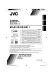
Block Diagram Model
Examine the model and its structure. The main model window contains the CR-CR
transmission subsystem, the input or driver shaft assembly, and the output or driven
shaft assembly. Each assembly consists of a driveline axis with applied damping and
inertia torques. Each driveshaft balances the torques applied across its ends with the
damping and inertia forces, thereby transmitting a net torque along the driveline.
The main model also includes a brake clutch. When this clutch is locked, the driven shaft
stops turning. This clutch must remain unlocked if the CR-CR transmission is engaged.
Main Model Window
What the Model Contains—Opening the Subsystems
Open each subsystem.
1-7
1
Introducing SimDriveline Software
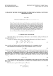
The CR-CR 4-Speed transmission subsystem contains four clutches, two planetary
gears, and four inertias (rotating bodies). Ignoring the reverse gear and its clutch, this
transmission has four possible (forward) gear settings. Exactly two clutches must be
locked at any one time for the transmission to engage and to avoid conflicting constraints
on the gear motions.
CR-CR 4-Speed Transmission Subsystem
The Clutch Control variant subsystem provides the pressures that lock the necessary
clutches. In its default state, the clutch controller is programmed to move the
transmission through a fixed sequence of gears, then unlock all the transmission
clutches. This control program allows the driven shaft to “coast” for a time, and then
engage and lock the brake clutch to stop the driven shaft.
1-8
Drivetrain Model
Clutch Control Subsystem
The Scopes subsystem provides Scope blocks to display the clutch pressure and the driver
and driven shaft velocity signals.
Scopes Subsystem
Run the Model
To display the CR-CR driveline model behavior:
1
Open the Scopes subsystem and then each of the Scope blocks. Close the Scopes
subsystem.
1-9
1
Introducing SimDriveline Software
1-10
2
Click Start. The model steps through the gears and then brakes.
3
Observe how the clutch pressure signals move the transmission into one gear
after another, at 0, 5, 10, and 15 seconds of simulation time. Compare these clutch
pressure signals to the clutch schedule in the CR-CR transmission subsystem to
determine which gear settings the model is implementing. The model steps through
gears 1, 2, 3, and 4, before coasting and then braking.
Drivetrain Model
1-11
1
Introducing SimDriveline Software
1-12
4
Compare the angular velocities of the driven and driver shafts. In the transmission,
the two planetary gears are coupled in different ways in the different gear settings,
producing different relationships between the driven and driver shaft velocities. The
effective drive ratio of output to input shafts is the reciprocal of the ratio of output to
input angular velocities.
5
Observe what happens at 20 seconds. The transmission clutch pressures drop to
zero, and the transmission disengages. The transmission ceases to transfer angular
motion and torque from the driver to the driven shaft, and the driven shaft continues
to spin from inertia alone. A small kinetic friction damping gradually slows the
driven shaft over the next 6 seconds.
6
At 26 seconds of simulation time, the brake clutch pressure begins to rise from zero,
and the brake clutch engages. The driven shaft decelerates more drastically now.
Between 26.0 and 26.2 seconds, the brake clutch locks, and the driven shaft stops
rotating completely.
Drivetrain Model
Modify the Model
You can modify this example model to explore other SimDriveline features. Here you
modify and rerun the model to investigate two aspects of its motion.
• Measure the effective drive ratio of the CR-CR transmission in each gear setting that
it steps through.
• Change the gear sequence.
Measuring the Drive Ratio of the CR-CR Transmission States
A transmission is a set of coupled gears. For a particular transmission gear setting, the
ratio of driven (output) shaft velocity to the driver (input) is fixed. Its reciprocal, the drive
ratio, is like a gear ratio of an individual gear coupling, but for the whole transmission.
Add and connect the necessary Simulink blocks to measure the drive ratio of the
transmission.
1
Open the Scopes subsystem.
2
From the Simulink library, copy into the Scopes subsystem:
• A Divide block from the Simulink Math Operations library.
• A Scope block from the Simulink Sinks library.
3
From the vDriver input signal, branch a signal line and connect it to the X inport on
the Divide block. From the vDriven input signal, again branch a signal line. Connect
it to the ÷ inport on the Divide block.
The output-to-input drive ratio is the ratio of input to output velocities.
4
Connect the outport of the Divide block to the Scope. Rename Scope to Drive Ratio.
1-13
1
Introducing SimDriveline Software
CR-CR 4-Speed Model with Drive Ratio Measurement
5
Open the Drive Ratio scope and restart the example. Observe how the drive ratio
steps through a sequence of five-second states, in parallel with the clutch pressures
and clutch modes, until it reaches 20 seconds. The drive ratio measurement after 20
seconds is not meaningful because the transmission is uncoupled.
Just after 26 seconds, the driven shaft velocity drops to zero, and the Divide block
produces divide-by-zero warnings at the MATLAB command line.
6
1-14
Consult the table, Clutch Schedule for the CR-CR 4-Speed Transmission. Check
the drive ratios for each gear, 1, 2, 3, and 4, in terms of the gear ratios of the two
Drivetrain Model
Planetary Gears in the transmission. Determine the numerical values for these drive
ratios for gear settings 1, 2, 3, and 4. Then check them against the values displayed
in the Drive Ratio scope.
The drive ratio sequence should be 3, 5/3, 1, and 2/3, respectively, for the first,
second, third, and fourth intervals of five seconds each.
Changing the Transmission Gear Sequence
When you first open the sdl_crcr example, the Clutch Control variant subsystem is
programmed to step through CR-CR gear settings 1, 2, 3, and 4, before disengaging.
Modify it to step through settings 1, 2, 3, and 1, then disengage. The fourth gear requires
that A to be free, B to be locked, C to be locked, and D to be free. You have to modify the
clutch pressure signal sequence from 15 to 20 seconds so that the transmission is set in
first, not fourth, gear. The first gear requires clutches A and D to be locked and clutches
B and C to be free.
1
Determine the clutch states that correspond to first gear. Refer to table Clutch
Schedule for the CR-CR 4-Speed Transmission.
2
Double-click Clutch Control.
3
In the Clutch Control subsystem, double-click Programmed.
4
In the Programmed subsystem, double-click Clutch Pressures. The signal builder
window opens with the clutch pressure signals.
5
In the time interval 15–20 seconds, update clutch signals A-D to match first gear.
Clutches A and D must lock, while clutches B and C must remain free. Specify a
signal value of one to lock a clutch, zero to unlock it.
1-15
1
Introducing SimDriveline Software
Modified CR-CR 4-Speed Transmission Clutch Pressures
6
Run simulation.
Clutch pressures, clutch modes, and driven shaft velocities in the time interval 15–
20 seconds now correspond to first gear. You can confirm this by referring to the
Drive Ratio plot for the updated model. The ratio has changed from 2/3 (fourth gear)
to 3 (first gear).
1-16
What You Can Do with SimDriveline Software
What You Can Do with SimDriveline Software
In this section...
“What SimDriveline Software Contains” on page 1-17
“Model Driveline Systems” on page 1-18
“Model Inertias and Gears” on page 1-19
“Model Dynamic Driveline Elements” on page 1-20
“Model Custom Driveline Elements” on page 1-20
“Actuate and Sense Motion” on page 1-20
“Simulate and Analyze Motion” on page 1-21
What SimDriveline Software Contains
SimDriveline software is a set of block libraries in the Simulink environment and based
on Simscape software. You connect SimDriveline blocks to normal Simulink blocks
through Simscape physical signal blocks that define physical units.
The blocks in the SimDriveline library and the related mechanical blocks in the Simscape
Foundation library are the elements to model driveline systems. These systems consist
of one or more inertias and masses, rotating about or translating along one or more axes,
constrained to rotate or translate together by gears, which transfer torque and forces to
different parts of the driveline. You can represent drivelines with components organized
into hierarchical subsystems, as in any Simulink model. You can:
• Constrain motion with gears
• Add complex dynamic elements such as clutches, clutch-like elements, and other
couplings
• Represent such vehicle components as bodies and tires
• Actuate bodies with torques, forces, and motions
• Integrate the Newtonian rotational and translational dynamics, then measure the
resulting motions
Relation to Simscape Software
To model and simulate physical systems, SimDriveline models use such Simscape
technologies as nondirectional physical connections and conserving ports, physical
1-17
1
Introducing SimDriveline Software
signals carrying physical units, custom component modeling, specialized solvers, and
data logging.
The Simscape mechanical rotational and translational domains form the basis of the
SimDriveline block libraries and models. The Simscape Foundation library itself
includes physical signal blocks; and basic mechanical blocks representing inertia, mass,
and simple mechanical couplings. It also includes motion, torque, and force sources and
sensors.
For more about modeling and simulating in the Simscape environment, see the
“Simscape”documentation.
Physical Connections, Mechanical Conserving Ports, and Physical Signals
On SimDriveline blocks, the mechanical conserving ports anchor physical connection
lines that, in this domain, represent mechanical axes. These axes are either rotation axes
along which torque is transferred and around which inertias rotate, or translation axes
along which force is transferred and along which masses translate.
Certain blocks defined in Simscape domains also require input or output signals that
carry physical units, or physical signals. Simscape physical signal lines and ports
represent and connect physical signals with units. Conversion blocks allow you to convert
dimensionless Simulink signals to Simscape physical signals, and back.
Model Driveline Systems
SimDriveline software extends Simulink and Simscape software with blocks to model
driveline components and properties, represent drivelines as physical networks, and to
solve the equations of motion.
To build and run a SimDriveline model representation of a driveline:
1
Specify rotational inertia or translational mass for each body. Connect the bodies
with physical connection lines representing driveline axes at mechanical conserving
ports.
If needed, ground the driveline to one or more mechanical references fixed in space.
2
1-18
Constrain the driveline axes to rotate or translate together by connecting them with
gears. Gears impose static constraints on driveline motions and transfer torques and
forces at fixed ratios.
What You Can Do with SimDriveline Software
3
As necessary, add dynamic elements that transfer torque, force, and motion among
driveline axes in a nonstatic way. These elements include internal torque-generating
components such as damped springs, clutches, clutch-like elements, transmissions,
and torque converters. You can also construct and connect your own dynamic
elements.
Similarly, add dynamic sources and environmental interactions, such as engines,
vehicle bodies, and tires.
4
Set up mechanical sources and sensors to initiate and record body motions, as well as
apply external torques and forces to the driveline.
5
Connect the Simscape Solver Configuration to the driveline, then configure it. Start
the simulation, calling the Simulink and Simscape solvers to find the motions of the
system. Display and analyze the motion.
Model Inertias and Gears
SimDriveline software defines a driveline as a collection of rotating and translating
bodies, defined by their rotational inertias and translational masses. Rotational and
translational degrees of freedom (DoFs) originate on inertias and masses, but are carried
by physical connection lines. Directly connecting one body to another constrains both
bodies to rotate at the same angular or linear velocity. A torque or force applied to one
body is applied to both. You can also ground driveline axes to mechanical references that
do not move and that represent infinite effective inertia or mass.
Note: All SimDriveline DoFs are absolute in an implicit global coordinate system at rest,
but are measured and used in a relative way, between one component and another. To
measure with respect to the global rest frame, ground sensors or other components with
mechanical reference blocks.
In a real driveline, the bodies can also be connected indirectly by gears that couple
driveline axes. The gears constrain the axes to rotate together. These gears can be simple
or complex and can couple two or more axes. The gears have two roles:
• Constraining the connected axes to rotate or translate together at velocities in fixed
ratio or ratios.
• Transferring the torques or forces flowing along one or more axes to other axes, also
in fixed ratio or ratios.
1-19
1
Introducing SimDriveline Software
Model Dynamic Driveline Elements
To create more realistic driveline models, you elaborate on simple drivelines consisting
of inertias, masses, and gears. You add complex mechanical elements that generate
torques and forces internally within the driveline, between one axis and another. Certain
SimDriveline blocks encapsulate as subsystems entire models of complex driveline
elements:
• Load-dependent loss models of nonideal gears
• Clutches and clutch-like elements that model the locking and unlocking of pairs of
driveline axes by applying kinetic and static friction.
• Vehicle component models that represent engines, tires, and vehicle bodies
• Specialized torque and force models, such as torque converters, hard stops, and
damped spring-like torsion
Model Custom Driveline Elements
The blocks provided in the Simscape Foundation library can serve as starting points for
developing variant or entirely new models to simulate the same components. You can
also study masked subsystems by looking under their masks. If necessary, break such a
block's library link before modifying it, and then create your own version. Or, create your
own completely new blocks using SimDriveline and Simscape components, or with the
Simscape language.
For more information on specialized driveline components, see “Specialized and
Customized Driveline Components”.
Actuate and Sense Motion
Simscape motion sources and sensors are the blocks that you use to insert and extract
basic kinematic and dynamic information:
• Source blocks impart motion to driveline axes and impose externally defined torques
and forces on the bodies of a driveline.
• Sensor blocks measure the motions of, and the torques and forces transferred along,
the axes of a driveline system.
Source inputs and sensor outputs are physical signals that carry units.
1-20
What You Can Do with SimDriveline Software
Simulate and Analyze Motion
Once you specify all the rotational inertias and translational masses of the bodies and
interconnect the bodies with gears and other driveline elements, the dynamical problem
of finding the system motion is solvable. To finish a driveline model and prepare it for
simulation, you must connect the driveline to the Simscape solver. This solver defines
certain aspects of the simulation and integrates the Newtonian dynamics for the system,
applying all internal and external torques and constraints to find the motions of the
bodies.
Once your model is ready for simulation, run it and analyze its motions, torques, and
forces.
Inverse Dynamics — Trimming and Linearization
In many cases, you do not know the torques and forces necessary to produce a given set
of motions. By motion-actuating your driveline with motion sources and measuring the
resulting torques and forces, you can find the torques and forces required to produce
specified motions. This technique inverts the canonical approach to dynamics, which
consists of finding motions from torques and forces.
A special case of inverse dynamics is trimming. This technique involves searching for
steady-state motions of the bodies, when their accelerations and the torques and forces
they experience vanish. Using the specialized tools in Simscape and Simulink, you can
perturb such a steady motion state slightly to find how the system responds to small
disturbances. The response indicates the system stability and suitability for controllers.
Generating Code — Real-Time and Hardware-in-the-Loop Simulation
SimDriveline software is compatible with Simulink Acceleration modes, Simulink Coder,
and Simulink Real-Time™ software. With these products, you can generate code versions
of the models the you originally create in Simulink with block diagrams, enhancing
simulation speed and model portability. A common application of generated code is
defining real-time and hardware-in-the-loop simulations.
The presence of clutches in a driveline model induces locking-unlocking iterations
and dynamical discontinuities. These discontinuities place certain restrictions on code
generation. For more information about these restrictions, see “Driveline Simulation
Performance” and “SimDriveline Limitations”.
1-21
2
Modeling Driveline Systems
The following sections introduce you to modeling drivetrains in the SimDriveline
environment. They start with describing how you access the SimDriveline block library,
then review the essential rules of connecting blocks and transferring motion, torque, and
force. The rest of the sections then move in a series of short tutorials, from representing
gears, through modeling clutches and transmissions, to end with simulating a full car.
• “SimDriveline Block Libraries” on page 2-2
• “Build a Driveline Model” on page 2-6
• “Basic Motion, Torque, and Force Modeling” on page 2-9
• “Driveline Actuation” on page 2-26
• “Gear Coupling Control with Clutches” on page 2-29
• “Gears, Clutches, and Transmissions” on page 2-38
• “Complete Vehicle Model” on page 2-51
2
Modeling Driveline Systems
SimDriveline Block Libraries
In this section...
“About the SimDriveline Block Library” on page 2-2
“Access SimDriveline Block Libraries” on page 2-2
“Use SimDriveline Block Libraries” on page 2-4
About the SimDriveline Block Library
SimDriveline software provides a set of block libraries to model driveline systems. This
section explains how to open these SimDriveline block libraries and describes the nature
of each library.
Note: Basic mechanical rotational and translational blocks are contained in the Simscape
Foundation library.
Access SimDriveline Block Libraries
There are several ways to open the SimDriveline block library.
You can access the blocks through the Simulink Library Browser. Open the browser by
clicking the Simulink button
the SimDriveline subentry.
2-2
. In the contents tree, expand the Simscape entry, then
SimDriveline Block Libraries
You can also access the blocks directly inside the SimDriveline library in several ways:
• In the Simulink Library Browser, under Simscape, right-click the SimDriveline
subentry. Then select Open SimDriveline Library.
• At the MATLAB command line, enter sdl_lib.
SimDriveline Library
The SimDriveline library displays several top-level block groups. You can expand each
library by double-clicking its icon.
2-3
2
Modeling Driveline Systems
The next section summarizes the blocks of each library and their use.
Use SimDriveline Block Libraries
The SimDriveline block library is organized into separate libraries, each with a different
type of driveline block.
Brakes & Detents
The Brakes & Detents library provides blocks that represent simple clutch-like elements
that limit the relative motion of driveline axes with sliding or locking Coulomb friction.
Clutches
The Clutches library contains blocks that represent various clutches, driveline elements
with external input controls, and a variety of geometries that couple driveline axes with
Coulomb friction that can lock them together.
Couplings & Drives
The Couplings & Drives library contains blocks that model simple components that
couple driveline axes, such as torsional damped springs, torque converters, and variable
ratio transmissions. These dynamic elements generate internal driveline torques.
Engines
The Engines library contains blocks modeling different types of engines as sources of
driveline motion.
Gears
The Gears library contains blocks that represent simple and complex gears, driveline
elements that couple distinct driveline axes and constrain their relative motions. The
2-4
SimDriveline Block Libraries
Gear blocks range from simple two-wheel gear couplings, to such complex multiwheel
and multiaxis gears as planetary and differential gears.
Sensors
The Sensors library contains blocks that sense dynamic variables, such as power,
between two driveline components.
Tires & Vehicles
The Tires & Vehicles library provides blocks that represent components of a full vehicle
beyond the drivetrain itself. It includes models of vehicle bodies and tires in contact with
the ground.
2-5
2
Modeling Driveline Systems
Build a Driveline Model
The example model in “Drivetrain Model” on page 1-5 illustrates a typical drivetrain
system that you can model with SimDriveline software. It also illustrates the key rules
for connecting driveline blocks to each other and the dual roles of Simscape physical
connection lines in driveline modeling. Within the Simscape mechanical domain:
• The across variable is angular or linear velocity, depending on the type of mechanical
ports you are connecting to, rotational or translational. Along any connection line, the
velocity is the same.
• The through variable is torque or force, depending on the type of mechanical ports you
are connecting to. Torques or forces are conserved along a connection line and always
sum to zero at line branch points.
Before building and running the tutorial models, you should review these rules.
• Driveline blocks feature mechanical conserving ports
and, in some cases, physical
signal ports
as well. You can connect mechanical ports only to other mechanical
ports, and physical signal ports only to one another.
You cannot mix rotational and translational ports, or connect a mechanical conserving
port to a physical signal port.
• The physical connection lines interconnecting mechanical ports represent driveline
axes and enforce physical relationships. Unlike physical signal and Simulink lines,
they do not represent signals or mathematical operations, and they have no inherent
directionality.
• A driveline connection line represents an idealized massless and perfectly rigid
spinning shaft or translating axis. A driveline connection line between two ports
constrains the two driveline components that are connected to the line to rotate or
translate at the same velocity.
• You can branch mechanical connection lines. You must connect the end of any branch
of a mechanical connection line to a mechanical port .
• Branching a driveline connection line modifies the physical constraints that it
represents. All driveline components connected to the ends of a set of branched lines
rotate or translate at the same velocity. For lines branched from a branch point, the
sum of all torques or forces flowing in equals the sum of all torques or forces flowing
out. How the torque or force is divided depends on the defining equations of the
attached blocks in the rest of the system.
2-6
Build a Driveline Model
• Mechanical connection lines satisfying the velocity constraint must have the same
initial velocities.
Branching Driveline Connection Lines
The Solver Configuration block in this example does not use any torque. It does share the
angular velocity constraint from the branch point. Symbolically, the branching conditions
on driveline connection lines are:
ω1 = ω2= ω3 ...
τ1 + τ2 + τ3 + ... = 0 .
The sign convention is that torques flowing in are positive. Like all driveline axes, these
have no inherent directionality. Torque flow directions are defined by overall system
equations during simulation.
Torque and motion are transferred through the driveline from some driveshafts to
others. Certain SimDriveline blocks require explicit directionality and represent it by
designating one driveline connector port as the input base (B) and the other as the output
follower (F), or some equivalent pair. When needed, positive relative motion of driveline
axes or shafts is measured as follower relative to base.
2-7
2
Modeling Driveline Systems
Motion Is Absolute Except when relative motion is explicitly required, all motion in
SimDriveline and Simscape models is measured in implicit absolute coordinates. The
Mechanical Rotational Reference and Mechanical Translational Reference blocks define
the absolute zero velocity. If they are connected to a driveline axis, these blocks enforce
this zero-motion state on that axis.
2-8
Basic Motion, Torque, and Force Modeling
Basic Motion, Torque, and Force Modeling
In this section...
“About Inertia, Motion, and Gears” on page 2-9
“Couple Rotational Motion with Gears” on page 2-9
“Couple Two Spinning Inertias with Simple Gear” on page 2-10
“Couple Two Spinning Inertias with Variable Ratio Transmission” on page 2-18
“Couple Three Spinning Inertias with Planetary Gear” on page 2-21
About Inertia, Motion, and Gears
The purpose of a gear set is to transfer rotational motion and torque at a known ratio
from one driveline axis to another. This section introduces you to modeling gears and
using them to couple bodies rotating on driveline axes.
Note: The concepts and examples of this section explain angular gears in relation to
rotational motion and torque. Analogous rules apply to linear gears, and translational
motion and force.
Couple Rotational Motion with Gears
A gear set consists of two or more meshed gears rotating together at some specified
gear ratios. By convention, SimDriveline gear ratios are constant. The gear ratios
determine how angular velocity and torque are transferred from one driveline component
to another.
Gear Coupling Rules
Ideal gears mesh and rotate together at a point of contact without frictional loss or
slippage.
The simplest gear coupling consists of two circular gear wheels of radii r1 and r2, spinning
with angular velocities ω1 and ω2, respectively, and lying in the same plane. Their
connected shafts are parallel and carry torques τ1 and τ2. The gear ratio of gear 2 to gear
1 is the ratio of their respective radii: g12 = r2/r1. The power transferred along either shaft
is ω·τ.
2-9
2
Modeling Driveline Systems
The gear coupling is often specified in terms of the number of gear teeth on each gear, N1
and N2. The gear ratio of gear 2 to gear 1 is then g12 = N2/N1 = r2/r1.
The fundamental conditions on the simple gear coupling of rotational motion are ω2/ω1 =
±1/g12 and τ2/τ1 = ±g12. That is, the ratio of angular velocities is the reciprocal of the ratio
of radii, while the ratio of torques is the ratio of radii. The transferred power, being the
product of angular velocity and torque, is the same on either shaft.
The choice of signs indicates that the gears can spin in the same or in opposite directions.
If the gears are external to one another (rotating together on their respective outside
surfaces), they rotate in opposite directions. If the gears are internal to one another
(rotating together with the outside of the smaller gear meshing with inside of the larger
gear), they rotate in the same direction.
Caution Gear ratios in driveline model blocks must be strictly positive. Vanishing or
negative gear ratios cause SimDriveline simulation to stop with an error at model
initialization. If you need to reverse the relative rotation direction of a shaft connected to
a gear, you can change the direction in the gear block dialog box.
Couple Two Spinning Inertias with Simple Gear
In this example, you couple two spinning inertias, first, along a single shaft (driveline
axis), so that they spin with the same angular velocity; then spinning along two shafts
and coupled by a gear so that they spin at different velocities; and finally, coupled by a
gear and actuated by an external torque, spinning at different rates and experiencing
different torques. You use the most basic Simscape mechanical and SimDriveline blocks,
such as Inertia, Simple Gear, and Solver Configuration.
Modeling Two Spinning Inertias
Create the first version of the simplest, nontrivial driveline model, two inertias spinning
together along the same axis. Open the SimDriveline, Simscape, and Simulink block
libraries and a new Simulink model window.
1
2
2-10
Drag and drop two Inertia, two Ideal Rotational Motion Sensor, two Mechanical
Rotational Reference, and two PS-Simulink Converter blocks into the model window.
From the Simscape Utilities library, drag a Solver Configuration block. Every
topologically distinct driveline block diagram requires exactly one instance of this
block.
Basic Motion, Torque, and Force Modeling
3
From the Simulink library, drag and drop a Scope, a Mux, and two pairs of Goto
and From blocks. Connect the blocks as shown in the following figures. The sensor
subsystems are arranged hierarchically.
Model with Two Spinning Inertias
2-11
2
Modeling Driveline Systems
Sensor Subsystem
4
5
2-12
Motion Sensor Subsystem
Open each Inertia block. In the Variables tab, select the Rotational velocity
checkbox and set the Value parameter to pi radians/second (rad/s). The connection
line between the two Inertia blocks requires them to have the same rotational
velocity.
Open the Scope block and start the simulation. The two angular velocities are
constant at 3.14 radians/second.
Basic Motion, Torque, and Force Modeling
Coupling Two Spinning Inertias with a Simple Gear
Now you modify the model you just created by coupling the two spinning inertias with a
simple, ideal gear with a fixed gear ratio.
1
From the SimDriveline block library, drag and drop a Simple Gear block into your
model. Open the block. Change the default follower-base gear ratio value to 1.
Change the Output shaft rotates menu to In same direction as input shaft and
click OK. The simple gear then represents two gear wheels rotating together at the
same rate in the same direction, with one wheel inside the other. Connect the blocks
as shown in the following figure.
2-13
2
Modeling Driveline Systems
Model with Two Spinning Inertias Coupled by a Gear
2
3
4
5
2-14
Leave the initial angular velocities at pi in the Inertia blocks.
Open the Scope and start the simulation. The two angular velocities are constant at
3.14 radians/second for both Inertias.
Change the Output shaft rotates menu back to In opposite direction to input
shaft. The simple gear then becomes two wheels rotating together in opposite
directions, with the two wheels meshed on their respective outer surfaces. Change
initial velocity in Inertia2 to -pi.
Restart the simulation. The two angular velocities are 3.14 and –3.14 radians/second
for Inertia1 and Inertia2, respectively. The second angular velocity is the same, but
with opposite sign, because the two bodies are spinning in opposite directions.
Change the Output shaft rotates menu again to In same direction as input
shaft.
Basic Motion, Torque, and Force Modeling
Torque-Actuating Two Coupled, Spinning Inertias
In the final version of the simple gear model, you actuate the inertias with an external
torque instead of starting them with fixed initial angular velocities. The external torque
varies sinusoidally. You can find a completed version of this model in the sdl_simple_gear
example model.
1
2
From the Simscape Foundation library, copy an Ideal Torque Source and two Ideal
Torque Sensor blocks, plus a Simulink-PS Converter block and another Mechanical
Rotational Reference block. From the Simulink library, drag and drop a Sine Wave
block and two more pairs of Goto and From blocks.
Connect the blocks as shown in the following figures. Note that the Torque Sensor
subsystems are arranged in parallel with the Motion Sensor subsystems inside the
Sensor subsystem blocks. Set the initial velocities of both Inertias to zero. Modify the
Scope block to add another axis for measuring the torques. Connect the other blocks
as shown.
2-15
2
Modeling Driveline Systems
Model with Two Spinning Inertias Coupled by a Gear and Actuated with Torque
2-16
Basic Motion, Torque, and Force Modeling
Updated Sensor Subsystem
3
Torque Sensor Subsystem
Open the Scope block and start the simulation.
The measured torques and angular velocities vary sinusoidally. As in the preceding
models, the angular velocity of Inertia2 is half that of Inertia1. The torque in the second
(follower) shaft is twice that in the first, as required by the laws of gear coupling.
If you change the Output shaft rotates menu to In opposite direction to input
shaft in Simple Gear and restart the simulation, the same angular velocities and torques
result, except that the values associated with Inertia2 and the second shaft are negative,
because the second body and second shaft are spinning in opposite directions.
2-17
2
Modeling Driveline Systems
Sensing and Actuating Motion and Torque
The mechanical sensor and source blocks that you use in the preceding models illustrate
their dual nature. They act as driveline components themselves, but also let you inject
and extract physical signals associated with motion and torque, including the correct
physical units. You can use these physical signals with other blocks in the Simscape
physical modeling environment, or convert them to dimensionless Simulink signals for
use in the nonphysical part of your model. Both sensor and source blocks have pairs of
mechanical ports and are connected either in series with or across physical connection
lines.
• Mechanical sensor and source blocks have both mechanical conserving ports
physical signal ports
and
.
Many SimDriveline blocks also feature a mix of mechanical conserving and physical
signal ports.
• An Ideal Torque Source injects torque along, or in series with, the driveline
connection line. An Ideal Torque Sensor measures the torque flowing along, or in
series with, the driveline connection line.
• An Ideal Rotational Motion Sensor reports the difference between the motions at its
two connection ports.
If you want to extract the absolute motion at its R port, connect the C port to a
mechanical reference block that grounds that port to zero motion.
Couple Two Spinning Inertias with Variable Ratio Transmission
You can modify the simple gear model further by replacing the fixed-ratio gear with a
transmission whose gear ratio varies in time. You specify the gear ratio variation with a
Simulink signal converted to a unitless physical signal. Start with the simple gear model
you built in the preceding section or by opening and editing the sdl_simple_gear example.
1
2
2-18
From the SimDriveline block library, drag and drop a Variable Ratio Transmission
block and replace the Simple Gear block with it. Open the Variable Ratio
Transmission block dialog box and make sure that the Output shaft rotates
parameter is set to In same direction as input (the default setting). The two
shafts will spin in the same direction. Ignore the other settings and close the block
dialog box.
The Variable Ratio Transmission block accepts the continuously varying gear ratio
as a physical signal Simulink signal through the extra physical signal input labeled
Basic Motion, Torque, and Force Modeling
r. For this example, create a variable signal for the gear ratio with a Signal Builder
block from the Simulink block library and Simulink-PS Converter block. Build a
signal that rises with constant slope from 1 to 2 over 10 seconds. Then connect the
converted physical signal to the r port.
2-19
2
Modeling Driveline Systems
3
2-20
Simple Variable Ratio Transmission Model
Do not change the other, original settings of the simple gear model. Open the Scope
and start the simulation.
Basic Motion, Torque, and Force Modeling
The angular velocities and torques of the two shafts have the same signs. The ratios of
angular velocities and torques start at 1, because the initial gear ratio is 1. As the gear
ratio increases toward 2, the angular velocity of Inertia2 becomes smaller than that of
Inertia1, while the associated torque in the second shaft becomes larger than that in the
first shaft. Because of the changing gear ratio, the motion and the torques are no longer
strictly sinusoidal, even though the actuating external torque is.
The sdl_variable_gear example is a full model of this type. To learn more about how to
use variable gear ratios, consult the Variable Ratio Transmission block reference page.
Couple Three Spinning Inertias with Planetary Gear
You can further modify the simple gear model and use it as a starting point for studying
more complex gear sets. One of the most important complex gear sets is the planetary
gear, which has three wheels, the ring, the sun, and the planet, all held in place by a
common carrier body. The planetary gear is important because it is a common component
in complex, realistic transmissions.
1
2
Replace the Simple Gear in your model with a Planetary Gear from the SimDriveline
block library. A planetary gear splits input angular motion from the carrier between
the ring and sun wheels, each connected to their respective bodies.
Copy another Inertia and two more Ideal Rotational Motion Sensors. Connect the
blocks to form the new diagram as shown in the following figure. In this example,
the torque source and the motion sensors are organized into the Torque Actuator and
Motion Sensor subsystems.
2-21
2
Modeling Driveline Systems
3
2-22
Simple Planetary Gear Model
Enter 2 for the Ring to sun teeth ratio in Planetary Gear. Open the Scope and
start the simulation to observe the angular velocities of the ring, carrier, and sun,
from largest to smallest. The ratio of the ring to sun gear velocities is always 2.
Basic Motion, Torque, and Force Modeling
4
5
To see the ring and sun wheels spinning alone, you must lock the carrier. In
this case, you switch the torque actuation to the ring wheel. Copy a Mechanical
Rotational Reference block from the Simscape Foundation library. Disconnect and
delete Inertia, replacing it on the carrier driveline axis with the reference block, and
reconnect the Solver Configuration block to this connection line.
Reconnect the Torque Actuator subsystem and Sine Wave block as shown in the
following figure.
2-23
2
Modeling Driveline Systems
6
2-24
Simple Planetary Gear Model with Locked Carrier
Open the Scope and start your model. Observe the angular velocities of the ring,
carrier, and sun.
Basic Motion, Torque, and Force Modeling
The carrier, connected to Mechanical Rotational Reference, does not move. The ring
is driven with a sinusoidal torque, and the sun responds by spinning in the opposite
direction (ring and sun gear wheels are external to one another) at twice the rate. The
ring wheel has twice the radius (or twice the number of teeth) as the sun, so it spins half
as fast.
2-25
2
Modeling Driveline Systems
Driveline Actuation
In this section...
“About Torques, Forces, and Motion” on page 2-26
“Actuate a Driveline with Torques and Forces” on page 2-27
“Actuate a Driveline with Motions” on page 2-27
“Set Initial Conditions of Driveline Motion” on page 2-28
About Torques, Forces, and Motion
From the torques and forces applied to driveline inertias and masses, a SimDriveline
simulation determines the resulting motion from the driveline component connections
and defining equations. However, a simulation can also accept motions imposed on a
driveline and solve for the torques and forces to produce those motions. In general, a
driveline simulation is a mixture of these two requirements, solving dynamics both
forward (torque and force to motion) and inverse (motion to torque and force). Imposing
motions and applying torques and forces to a driveline are together forms of mechanical
actuation.
This section describes how to actuate drivelines with torques, forces, and motions, as
well as how to set motion initial conditions. All of these actuation types (except for initial
conditions) require physical signal inputs to define time-varying functions that carry
physical units.
Torque-Force Actuation and Motion Actuation Are Complementary and Mutually Exclusive
In all cases, you should exercise care as you apply a mixture of actuation types to a
driveline and its degrees of freedom (DoFs). The complete effect of the actuation types
must be such that:
• Driveline DoFs actuated by torques and forces are not also subject to motion
actuation. (They can be subject to motion initial condition settings.)
• Driveline DoFs actuated by motions are not also subject to torque or force actuation.
For a SimDriveline model to successfully simulate nontrivial motion, torque and motion
actuation types must exactly complement one another to account consistently for the
motion of all the DoFs. If this criterion is not satisfied, one of these outcomes results:
2-26
Driveline Actuation
• The motion of the driveline is trivial, staying in its initial motion state for the entire
simulation.
• The actuation types are inconsistent with each other, and the simulation stops with
an error.
• The actuation types leave the driveline motion underdetermined or overdetermined,
and the simulation stops with an error.
For more about driveline simulation errors, see “Driveline Simulation Errors” on page
4-7.
Actuate a Driveline with Torques and Forces
You can apply a torque to a rotational driveshaft, or a force to a translational driveshaft,
in the following ways:
• Directly, with a Ideal Torque Source or Ideal Force Source block.
• Indirectly, with a dynamic element that generates torque or force. Such blocks include
torque converters, clutches and clutch-like elements, and engines.
A torque or force source accepts a physical signal input and originates, from its
mechanical conserving port, a mechanical connection line carrying that torque or force.
The SimDriveline simulation solves for the motion of the spinning or sliding driveshaft,
given the torque or force that it is subject to. Therefore you cannot also subject that same
driveshaft to motion actuation.
Note: A driveline actuated by a torque must have a nonzero inertia, represented by
one or more connected Inertia blocks. A torque-actuated driveline without any inertia
experiences a singular acceleration. (The analogous restriction holds for force actuation,
masses, and Mass blocks.) In this case, the SimDriveline simulation stops with an error.
Actuate a Driveline with Motions
You can apply a motion to a driveshaft directly, with an Ideal Angular Velocity Source or
Ideal Translational Velocity Source block.
A motion source accepts a physical signal input and originates, from its mechanical
conserving port, a mechanical connection line spinning or sliding with the specified
motion.
2-27
2
Modeling Driveline Systems
The SimDriveline simulation solves for the torque or force carried by the spinning
or sliding driveshaft, given its motion. Therefore you cannot also subject that same
driveshaft to torque or force actuation.
Set Initial Conditions of Driveline Motion
When driveline simulation starts, the complete driveline determines the initial motion
of all driveshafts by a combination of constraints, motion sources, and initial condition
settings. You set the initial conditions for the rotational and translational motion of
inertias and masses in their respective Inertia and Mass blocks. The block default for
initial velocities is zero (no initial motion).
For more information about constraints and degrees of freedom, see “Driveline Degrees of
Freedom” on page 4-10.
Note: You must ensure that whatever initial conditions you impose on the Inertia and
Mass blocks in your driveline are consistent with all of the driveline's constraints and
motion sources. If an inconsistency occurs, SimDriveline simulation stops with an error
at model initialization.
Resolving Undetermined Motions in Complex Gears
A simple gear has two ports and imposes one constraint between them, leaving one
independent DoF. Once one port is connected to a driveshaft, the motion of the other
port's driveshaft is determined.
A complex gear has three or more ports and imposes one or more constraints among
them. A complex gear can have any number of independent DoFs, including none.
If a simulation apportions the initial motions of a complex gear in an unsatisfactory way,
determine how you want the overall initial motion divided up and enforce that division
by setting initial conditions on the connected Inertia and Mass blocks.
However you divide the initial motion among the gear shafts, ensure that this division is
consistent with all constraints in your driveline, as well as any motion sources.
For more information about complex gears, see “Basic Motion, Torque, and Force
Modeling” on page 2-9.
2-28
Gear Coupling Control with Clutches
Gear Coupling Control with Clutches
In this section...
“About Motion, Gears, and Clutches” on page 2-29
“Engage and Disengage Gears with Clutches” on page 2-29
“Brake Motion with Clutches” on page 2-34
“Model Friction Clutches at a Fundamental Level” on page 2-37
About Motion, Gears, and Clutches
An important requirement of a practical drivetrain is the ability to transfer rotational
motion and torque among spinning components at different speeds and gear ratios. In
general, a single set of gears is not sufficient to accomplish this transfer. Clutches allow
the drivetrain to selectively transfer motion, torque, and force at different gear ratios
under manual or automatic control.
This section explains how to model and use clutches in driveline models without and
with frictional losses and braking. On modeling various types of clutches and clutch-like
elements, as well as clutch control, see “Specialized Clutches” on page 3-11.
Engage and Disengage Gears with Clutches
A common problem in drivetrain design is transferring motion and torque at different
fixed gear ratios. Drivetrains are typically designed to switch among a set of distinct
gear ratios. Implementing the switch from one gear ratio to another requires gradually
disengaging one set of driveline couplings and engaging another set. Clutches allow you
to gradually engage and disengage driveline shafts from one another.
The Disk Friction Clutch block represents a standard surface friction-based clutch
that models this behavior. You also can model clutches in greater detail using the
Fundamental Friction Clutch block, which requires you to specify the static and kinetic
clutch friction more completely. See also “Model Friction Clutches at a Fundamental
Level” on page 2-37.
Note: You can model continuous motion-torque transfer with the Torque Converter block,
which simulates fluid viscosity instead of surface friction and never locks.
2-29
2
Modeling Driveline Systems
How a Clutch Works
A clutch makes two shafts spinning at different rates spin at a single rate by applying
forces that tend to accelerate one shaft and decelerate the other. The most common way
for a clutch to accomplish this action is with surface friction. Such a clutch can operate in
one of these modes of motion:
• Disengaged: the clutch applies no friction at all.
• Engaged but unlocked: the clutch applies kinetic friction, and the two shafts spin at
different rates.
• Engaged and locked: the clutch applies static friction, and the two shafts spin
together.
A clutch consists of mated frictional surfaces overlapping one another and connected on
either side to a shaft. If the clutch is disengaged, the frictional surfaces have no contact
and the shafts spin independently. To engage the clutch, contact between two surfaces is
induced by applying clutch pressure (a force normal to the surfaces). The two surfaces in
contact and moving relative to one another experience kinetic friction, which causes them
to narrow their relative velocity. The friction acts to reduce the relative motion between
the two clutch plates and their connected shafts. At some critical combination of reduced
relative speed and pressure (normal force), the clutch locks, so that the two shafts are
spinning at the same rate. The shafts remain locked together as long as the transmitted
torque remains less than the static friction, which is proportional to the applied normal
force. If the clutch unlocks but is still engaged, it again applies kinetic rather than static
friction.
The transition between unlocked and locked states is discontinuous. Modeling a clutch
locking or unlocking event requires searching for the correct combination of pressure
and torque acting on the clutch. The locking and unlocking events are determined during
simulation by repeated and accurate zero-crossing detection. On simulating events and
solving constraints together with dynamics in Simscape models, see “Simulation”.
Engaging and Disengaging a Gear with a Clutch
Construct a simple model that simulates a gear being engaged, then disengaged, by a
clutch. Torque and motion are transferred from one shaft to another over a finite time
interval. You can start with the simple gear model created in the preceding section or
with the sdl_simple_gear example, creating a simpler version with the Disk Friction
Clutch.
A more complex version, shown here, is the sdl_simple_clutch example. It uses a clutch
subsystem containing the Fundamental Friction Clutch instead.
2-30
Gear Coupling Control with Clutches
Simple Clutch Model with Programmed Clutch Pressure
Custom Clutch Subsystem
2-31
2
Modeling Driveline Systems
• The clutch subsystem is positioned between Inertia1 and Simple Gear and reports the
clutch mode (forward, reverse, locked).
• The PS Constant block replaces the sinusoidal signal as the torque input. The torque
sensor blocks are omitted.
• Simulink-PS Converter and PS-Simulink Converter blocks communicate between
physical signals in the Simscape environment and Simulink blocks such as Signal
Builder and Scope.
• The Signal Builder block provides the programmed clutch pressure signal, normalized
between 0 and 1, as shown in the following table. This signal is converted to a
physical pressure inside the clutch subsystem.
Time Range (Seconds)
Signal Value
0–2
0
2–4
0 – 0.8 with constant slope
4–6
0.8
6–7
0.8 – 0 with constant slope
7 – 10
0
Open the Scopes and start the simulation. The normalized clutch pressure signal follows
the profile that you created in Signal Builder and determines the model's behavior.
1
From 0 to 2 seconds, the velocity of Inertia1 increases linearly because it is subject to
a constant torque.
2
At 2 seconds, the clutch begins to engage, and Inertia2 begins to spin. The velocity
of Inertia1 continues to rise, although at a slower rate, because the two inertias now
share the external torque.
3
At 4 seconds, the pressure reaches its maximum. At about 5.32 seconds, the clutch
locks. The driveshafts connected by the clutch now spin together. Inertia1 and
Inertia2 continue to speed up at constant accelerations, Inertia2 at half the velocity
of Inertia1.
4
At 6 seconds, the clutch begins to disengage as the pressure drops. Inertia1 and
Inertia2 continue to accelerate with the applied torque.
The clutch unlocks at about 6.73 seconds and fully disengages at 7 seconds.
(The clutch unlocks a little before completely disengaging because the pressure,
even before vanishing, becomes too small to maintain the lock.) Inertia1 is still
2-32
Gear Coupling Control with Clutches
accelerating. But Inertia2, now free of the driveshaft and its torque, no longer
accelerates and instead spins at a constant rate without frictional loss.
While the two shafts are locked, between 5.32 and 6.73 seconds, Inertia1 and Inertia2
spin in a fixed 2:1 ratio, because of the Simple Gear.
How the Clutch Mode Indicates Locking and Unlocking
The Clutch mode signal indicates the relative motion of its two connected shafts. From 0
to 5.32 seconds, the two shafts are moving relative to one another. The follower (driven)
2-33
2
Modeling Driveline Systems
shaft is slower than the base (drive) shaft, so the mode signal is –1. Once the two shafts
lock, their relative velocity is 0, and the mode signal switches to 0. At 6.73 seconds, they
unlock, and the drive (base) shaft starts accelerating faster than the driven (follower)
shaft. The mode signal switches back to –1.
Brake Motion with Clutches
A special case of transferring motion occurs when you want to brake the spinning of
a driveline component, slowing it down until it stops. The common way to brake the
motion is to couple the spinning component to a rotational ground. You can represent
a rotational ground with a Mechanical Rotational Reference block from the Simscape
Foundation library. Because a rotational ground cannot move, a driveline axis locked to
a rotational ground also cannot move. You can implement the gradual engagement or
disengagement of a driveline component with a rotational ground using a clutch, just as
you use a clutch to gradually couple or uncouple two spinning shafts.
Braking with a Double-Clutch System
The sdl_clutch_engage example model builds on the preceding tutorial models and
features two clutches, one of which acts as a brake. The model also includes frictional
damping for greater realism. The simulation time is set to inf (infinity). For simplicity,
the Disk Friction Clutch block is used.
2-34
Gear Coupling Control with Clutches
Simple Clutch Model with Brake Clutch
This model uses the basic structure of inertia—clutch—gear—inertia. The first body,
Inertia1, is driven by an external torque, and the initial velocities are 0. There is,
however, another clutch for the second body, Inertia2, that can couple Inertia2 to the
Mechanical Rotational Reference and bring it to a stop. Another new feature is the
switching assembly based on the clutch switch. You can change this switch to apply a
constant clutch pressure signal to either clutch 1 (the gear clutch) or clutch 2 (the brake
clutch). (The Fcn 1–u block ensures that the full clutch pressure is applied to either one
or the other, but not both at once.) The Damper blocks apply viscous (velocity-dependent)
friction to the spinning of Inertia1 and Inertia2.
1
Start the model with the Clutch Switch set to 1. The clutch pressure is then applied
to the Gear clutch, which engages and locks the driver and driven shafts and causes
them to rotate at the same velocity.
Inertia2 is on the other side of the Simple Gear. The angular velocity of Inertia1 is
twice that of Inertia2 because the gear ratio of the Simple Gear block is 2, follower
2-35
2
Modeling Driveline Systems
to base. In this switch mode, no clutch pressure is applied to Brake Clutch, which
remains unengaged.
After an initial transient, the system settles into a steady state of motion where the
external torque balances the friction losses.
2
With the simulation running, change the Clutch Switch to 0 to disengage the gear
clutch and engage the brake clutch. The system undergoes another transient while
the Gear clutch disengages and Brake clutch engages.
The angular velocity of Inertia1 and the driver shaft settles down to a new steady
state of 10 radians/second, twice its old speed.
Because the Gear clutch is now disengaged, the driven shaft and Inertia2 are no
longer subject to a driving torque through Gear clutch. But the Brake clutch is
engaged and couples Inertia2 to the immobile Mechanical Rotational Reference.
Once engaged, the kinetic friction of the Brake clutch brings the driven shaft and
Inertia2 to a stop.
To see the transient behavior at simulation start and when you switch the clutches:
1
Start the simulation and let it run for a short time. Then switch Clutch Switch to the
other mode.
2
After a short time, stop the simulation. Use the Autoscale feature of the Scopes to
capture the entire simulation sequence. The transients from the starting behavior
and the switching transition are visible.
For example, in these plots, the model was started with Clutch Switch set to 1 (Gear
clutch locked, Brake clutch disengaged, no braking). The velocities quickly climbed to
their steady-state values. Then Clutch Switch was changed at about 1830 seconds of
simulation time. Gear clutch disengaged and Brake clutch engaged, braking Inertia2.
The driver shaft's angular velocity rose from 5 to 10 radians/second. The driven shaft's
angular velocity dropped from 5 to 0, and Inertia2's angular velocity dropped from 2.5 to
0.
2-36
Gear Coupling Control with Clutches
Model Friction Clutches at a Fundamental Level
The Disk Friction Clutch block requires only a single pressure signal to modulate the
kinetic friction. You fix all its other characteristics before starting simulation.
Modeling a friction clutch at a fundamental level requires direct control over the kinetic
and static friction torques. The Fundamental Friction Clutch block gives you that control.
With this block, you must specify, by either external signals or internal dynamics, the
clutch's kinetic friction and static friction limits (positive and negative) as functions of
time.
2-37
2
Modeling Driveline Systems
Gears, Clutches, and Transmissions
In this section...
“About Gears, Clutches, and Transmissions” on page 2-38
“Model a Two-Speed Transmission with Braking” on page 2-39
“Model a CR-CR 4-Speed Transmission Driveline with Braking” on page 2-45
About Gears, Clutches, and Transmissions
In a real drivetrain, you couple an input or drive shaft to one of many output or driven
shafts, or to one driven shaft with a choice of several gear ratios. The drivetrain then
requires several clutches to switch between gears. You couple one of the driven shafts or
one of the gear sets by engaging one of the clutches. You then switch to another output
shaft or another gear ratio by disengaging one clutch and engaging another.
You can also engage more than one clutch at a time to use multiple gear sets
simultaneously. Transmissions engage multiple gear sets at the same time to produce
a single effective gear ratio, or drive ratio. Changing gears requires disengaging one
set of clutches and engaging another set. You can specify the set of clutches to engage
and disengage for each gear ratio in a clutch schedule. Designing a clutch schedule
and shaping and sequencing the clutch pressure signals frequently constitute the most
difficult part of transmission design. A realistic transmission model must also include
losses due to friction and imperfect gear meshing.
This section explains how to model transmissions, by creating a transmission model from
gears and clutches. A predesigned transmission, the CR-CR 4-speed transmission, is the
basis of a second example.
Some Important Transmission Design Principles
When creating or modifying a transmission model:
• Connect inertia blocks with nonzero inertia values to gear shafts for realistic
simulation and preventing acceleration singularities when torques are applied.
• Make sure that the clutch schedule for your transmission specifies those clutches that
must be engaged and those that must be free at any instant for the transmission to
be properly in gear. Set all clutch pressures to 0 only if you want to disengage the
transmission completely (place it in neutral).
2-38
Gears, Clutches, and Transmissions
Do not engage any more or fewer clutches than needed, at any time during
simulation.
• If you want to redesign a transmission by adding or removing gears, you must
consider whether you also need to add or remove clutches and redesign the clutch
schedule. You also might need to add or remove gear shaft inertias.
On the relationship clutch pressure signals to solver choices and settings, see “Driveline
Simulation Performance” on page 4-2.
Model a Two-Speed Transmission with Braking
The example model sdl_simple_transmission contains a driveline system that makes up a
simple yet complete transmission.
2-39
2
Modeling Driveline Systems
Simple Transmission with Two Gear-Clutch Pairs and Braking
The model is built on the sdl_clutch_engage example model. This model contains two
driveline shafts or axes, with a constant actuating torque of 1 newton-meter applied
to the driver shaft. Both the driver and the driven shafts are subject to small viscous
damping torques (blocks D1 and D2). The viscous torque constant μ is 0.001 newtonmeters/(radians/second). In the steady state, the driving and damping torques balance
one another; the two shafts spin at constant rates, the driver shaft at (1 N-m)/(0.001 Nm/(rad/s)) = 1000 rad/s. (If braking is engaged, the driven shaft is stopped.) There are
now two selectable gears to couple the two axes, instead of one. (On modeling viscous
losses with nonideal gear bearings instead of dampers, see “Specialized Gears” on page
3-7.)
This transmission model couples the gears in a simple way, with each gear and the
brake associated with its own respective clutch. Coupling one gear requires engaging
2-40
Gears, Clutches, and Transmissions
and locking its corresponding clutch, while ensuring that the other two clutches are
disengaged. The brake clutch is directly activated by its own switch.
Setting Up the Gears, Clutches, and Brake
The two gears are Simple Gear blocks with different gear ratios, each connected in
series with its corresponding clutch. The two gear-clutch pairs are coupled in parallel.
This parallel assembly then couples the driver shaft to the driven shaft, with their two
spinning inertias. One gear is a “low” gear, the other a “high” gear. Following common
usage for automobile gears, the “low” and “high” labels refer to the angular velocity
ratios.
Note: The ratio of speeds in a gear is the reciprocal of the gear ratio.
• The low gear is the Simple Gear 5:1 block, which can be coupled by engaging its
corresponding clutch, modeled by the Low gear clutch block. The gear ratio is 5:1,
so that the ratio of output to input (follower to base) angular speeds is 1/5. Such a
gear has a high torque transfer ratio of 5, from base to follower. In an automobile, a
low gear like this is used to accelerate the vehicle from a stop by transferring a large
torque down the drivetrain from the engine.
• The high gear is the Simple Gear 2:1 block, coupled by engaging its own clutch,
represented by the High gear clutch block. The gear ratio is 2:1, and the angular
velocity ratio of follower to base is 1/2, or 5/2 times the ratio in the low gear. The
torque transfer ratio is only 2 from base to follower. An automotive high gear is used
for milder acceleration or coasting once a vehicle is moving at a significant speed.
The vehicle acceleration generated by this gear is less than that generated by the low
gear.
Switching on either the Neutral switch or the Brake switch disengages both gear
clutches. In either case, the driver shaft continues to spin, approaching a steady velocity,
subject to the competing driving and damping torques.
• Switching the transmission to neutral leaves the brake clutch disengaged and the
driven shaft free to spin. But without a driving torque, damping gradually brings the
driven shaft to a stop.
• Switching the brake on immediately locks the brake clutch and stops the driven shaft.
2-41
2
Modeling Driveline Systems
This simple transmission is based on mapping each transmission state one-to-one with
an engaged clutch. You cannot engage more than one clutch at a time without creating
conflicts between gear ratios or between the driver shaft and the rotational ground.
Controlling the Transmission State with a Clutch Schedule
The requirement to engage a certain clutch or set of clutches and disengage others, both
to implement transmission functions and to avoid motion conflicts between gears, is the
basis for all clutch schedules. Simulink provides a number of ways to implement clutch
schedules, depending on the complexity of the transmission and how much realism you
require for the clutch pressure signals.
Caution You must check every transmission's clutch schedule to implement its
transmission states correctly and to avoid motion conflicts among gear sets. You must
also check clutch pressure signal profiles to make sure that any transmission's clutches
are engaged, locked, unlocked, and disengaged in a realistic and conflict-free manner.
Unphysical or conflicting clutch schedules and clutch pressure signals lead to simulation
errors in SimDriveline models and can damage or destroy a real transmission.
For the sdl_simple_transmission model, avoiding such conflicts leads to a unique clutch
schedule.
Clutch Schedule for the Simple Two-Speed Transmission
Transmission State
Brake Clutch State Low Gear Clutch State
High Gear Clutch State
Neutral/Braked
Disengaged/
Locked
Disengaged
Disengaged
Low Gear
Disengaged
Locked
Disengaged
High Gear
Disengaged
Disengaged
Locked
The model contains a simple Clutch Control subsystem to implement the clutch schedule
and to output the clutch pressure signals to lock each clutch as needed.
2-42
Gears, Clutches, and Transmissions
Clutch Control Subsystem for Simple Transmission Model
In this simplified and unrealistic clutch control model, the clutch pressure signals are
constants: 1 to engage and lock a clutch; 0 to disengage it. (A clutch pressure signal
is normalized to equal 1 when the surface friction force equals the peak normal force
specified in the clutches.) For each transmission state, the table of these constants is
contained in the Clutch Schedule Table block, customized from the Direct Lookup Table
(n-D) block. Open the Clutch Schedule Table block to see this table.
2-43
2
Modeling Driveline Systems
The table is indexed in both row and column, starting from zero. An input signal of
0 causes the block to output the first column of table values; a value of 1 outputs the
second column; a value of 2, the third column. The Terminator block prevents the
first element of each column (that is, the entire first row of values) from leaving the
subsystem.
The first column applies zero pressure to the two gear clutches. The second column
applies full pressure to the low gear clutch and zero pressure to the high gear. The third
column applies full pressure to the high gear clutch and zero pressure to the low gear.
These different table columns are activated by changing the positions of the Gear switch
and Neutral switch, while leaving the Brake switch off. With the neutral switch off, the
Gear switch signal can pass to the Clutch Schedule Table. This signal is 1 for the low
gear and 2 for the high gear. Turning the neutral switch on prevents the Gear switch
signal from reaching the clutch controller.
Turning on the Brake switch also prevents the Gear switch signal from reaching the
clutch controller. At the same time, switching on the brake directly applies locking
pressure to the Brake clutch.
Running the Model, Switching Gears, and Braking
To see how gear switching works:
1
Start the model and open the two scopes.
Its initial transmission state is low gear, with the Gear switch to the left,
transmitting a signal value of 1. The driven shaft spins at one-fifth the rate of the
driver shaft, in the opposite direction.
2
Change the Gear switch from low to high (left to right, signal value of 1 to 2), and
observe how the driven shaft velocity increases in the Speeds and torques scope.
The driven-to-driver ratio is now one-half. (The driver shaft velocity decreases
slightly, because it experiences the damping torque on the driven shaft differently
depending on which gear is engaged.)
3
Change the Gear switch back to low (right to left, 2 to 1), then observe that the
driven shaft again spins more slowly.
At the same time, while you switch the gears back and forth, the clutches, as shown
in the Clutch modes scope, switch from Low gear clutch being locked, to the High
gear clutch being locked, and back. When one is locked, the other is unlocked.
2-44
Gears, Clutches, and Transmissions
4
Apply immediate braking by switching the Brake switch to on (left to right, 0 to
1). The driven shaft comes to an immediate and complete stop. The driver shaft
continues to spin.
Then release the brake, moving the Brake switch to off (right to left, 1 to 0).
5
Change the Neutral switch to the right position, transmitting a signal value of 0.
The two gear clutches unlock and disengage. The Brake clutch remains unengaged.
The driven shaft, subject to very light damping, now slows gradually.
6
By turning the Brake switch to on, you can switch the Brake clutch to the locked
mode and bring the driven shaft to a stop. The driver shaft continues to spin.
Adding Realistic Clutch Signals
The clutch control subsystem of this example is adequate for a simple model, but not
realistic. It contains unrealistic clutch pressure signals that rise and fall sharply. A full
clutch control model requires realistic clutch pressure signals that rise from and fall back
to zero in a smooth way. Greater realism requires a potentially more complex model. It
is critical for the Simscape and Simulink solvers to determine transmission motion for
exactly two clutches to always remain locked, or for all four to be unlocked, at any time
in the simulation. Changing the transmission's gear settings while maintaining this
requirement is an example of the central problem of transmission design.
For transmission and car examples with smoothed clutch pressure signals, see “Model a
CR-CR 4-Speed Transmission Driveline with Braking” on page 2-45 and “Complete
Vehicle Model” on page 2-51.
Model a CR-CR 4-Speed Transmission Driveline with Braking
The sdl_crcr example model builds on the previous clutch and transmission models
with a more realistic transmission. It uses a CR-CR 4-Speed transmission subsystem to
transfer motion and torque from one shaft and inertia to another.
2-45
2
Modeling Driveline Systems
CR-CR 4-Speed Transmission Model
A Torque Driver subsystem feeds a constant driving torque from a torque source to the
driver shaft (Inertia1). Two damping subsystems apply heavy and light viscous friction
to the driver and driven shafts, respectively. The two Scopes measure the shaft velocities
and clutch pressures, respectively. The model pre-load function defines essential
parameters in the workspace. (You can view this pre-load function. Open the model File
> Model Properties > Model Properties dialog box. Then, click the Callbacks tab).
The CR-CR 4-Speed transmission subsystem couples the driver to the driven shaft
(Inertia2). If the transmission is disengaged, a brake clutch and fixed housing allow you
to brake the driven shaft. When you first open the model, the Clutch Control subsystem
contains a set of programmed clutch signals for shifting the CR-CR transmission through
a preconfigured gear and braking sequence over 30 seconds.
For clarity, the model's major signal buses have been bundled as vectors and directed
using Goto and From blocks. The Scopes are collected in the Scopes subsystem for
convenience.
Replacing Programmed with Manually Controlled Clutch Pressures
The model represents the clutch control system using a Variant Subsystem block. This
block provides two clutch control modes, or variants: manual and programmed. To switch
to manual control mode:
1
2
3
2-46
Right-click Clutch Control.
In the context menu, select Variant > Override using > Variant1 (Manual)
Double-click Clutch Control and then Manual. During simulation, the Manual
subsystem provides direct control over gear changes.
Gears, Clutches, and Transmissions
4
5
In the Simulink toolbar, change the simulation time to inf.
Run simulation.
To change gears during simulation, use the Manual Switch blocks. Bit 2 Switch controls
clutches A and B, while Bit 1 Switch controls clutches C and D. The table summarizes
the clutch responses when toggling a switch up or down.
Manual Switch Block
Switch-Up Response
Switch-Down Response
Bit 2 Switch
Lock clutch A, release clutch Release clutch A, lock clutch
B
B
Bit 1 Switch
Lock clutch D, release
clutch C
Release clutch D, lock clutch
C
Manual Clutch Control for CR-CR Transmission
Configuring the CR-CR Transmission Subsystem
The CR-CR 4-Speed transmission subsystem uses certain parameters set to realistic
values. These parameters are referenced to variables defined in the workspace when the
model opens. These variables are used in the four CR-CR Clutch blocks A, B, C, and D.
CR-CR 4-Speed Transmission Clutch Variables
Workspace
Variable
Description
num_fric_surf Number of frictional surfaces in each clutch
eff_tor_rad
Effective torque radius in each clutch (m)
2-47
2
Modeling Driveline Systems
Workspace
Variable
Description
peak_normal
Peak normal force on clutch surfaces (N)
fric_coeff
(matrix)
Kinetic friction coefficient as a function of the relative angular velocity of the
clutch shafts
The clutch schedule of the CR-CR transmission subsystem is a table of gear settings,
clutch lockings, and gear ratios. There are four distinct (forward) gear settings, each with
a different effective gear ratio. For the transmission to be properly engaged and transmit
torque and motion, exactly two clutches must be locked at any instant. Unlocking all
the clutches simultaneously puts the transmission into neutral (no motion or torque
transfer). The transmission contains two planetary gears, five clutches, and four inertias.
Clutch Schedule for the CR-CR 4-Speed Transmission
Gear
Setting
Clutch A
State
Clutch B
State
Clutch C
State
Clutch D
State
Clutch R
State
Drive Ratio
1
L
F
F
L
F
1 + go
2
L
F
L
F
F
1 + go/(1 +
gi)
3
L
L
F
F
F
1
4
F
L
L
F
F
gi/(1 + gi)
Reverse F
F
F
F
L
–gi
• L = locked
• F = free
• gi = Input Planetary Gear ring-to-sun gear ratio
• go = Output Planetary Gear ring-to-sun gear ratio
The main model's Damping subsystems use these variables for frictional damping of the
driving (engine) and driven shafts coupled across the transmission.
Drive Shaft Damping Coefficients
2-48
Workspace Variable
Description
eng_damping
Driver (engine) shaft kinetic friction coefficient (N-m/(rad/
s))
Gears, Clutches, and Transmissions
Workspace Variable
Description
driven_damping
Driven shaft kinetic friction coefficient (N-m/(rad/s))
Programming the Clutch Schedule Logic
For this and the following sections, switch the default programmed Clutch Control
subsystem to the manually controlled configuration. See “Replacing Programmed with
Manually Controlled Clutch Pressures” on page 2-46.
From the main model, open the Clutch Control subsystem. The Clutch Schedule Logic
block provides the CR-CR 4-Speed clutch schedule as a truth table for the four forward
gears. Each row represents a different gear setting. You select a particular row for output
by inputting a set of 1s and 0s that specify the row value as a binary number.
CR-CR 4-Speed Clutch Schedule Logic
Gear Setting
Truth Table Row
Truth Table Value
1
002 = 0
10010
2
012 = 1
10100
3
102 = 2
11000
4
112 = 3
01100
In the order of the CR-CR Clutches—A, B, C, and D, respectively—the sequence of 1s and
0s indicates which clutches are locked (1) and which are free (0). These Boolean values
are then converted into normalized clutch pressure signals. The fifth value in each row
represents the disengaged reverse gear Clutch R.
Programming the Reverse Gear
By default, the Forward/Reverse Switch is set to the up position, placing the
transmission in forward motion. If you want to engage the reverse gear, set the switch to
the down position.
Open the corresponding Reverse block to see the reverse gear clutch schedule as a truth
table.
CR-CR Reverse Gear Clutch Schedule Logic
Gear Setting
Truth Table Value
Reverse
00011
2-49
2
Modeling Driveline Systems
Running the CR-CR Transmission Model — Changing Gears
You are now ready to run the model.
1
Open the Scopes subsystem, then the individual Scope blocks. Close the Scopes
subsystem.
With the Scopes, you can observe the angular velocities of the driving and driven
shafts, and the input pressures of the four clutches.
2
Open the Clutch Control subsystem, which should be set to manual control. Ensure
that the Forward/Reverse Switch is set to up and the Neutral Switch is set to down.
Also ensure that the simulation time is inf.
3
Start the model. You can change the forward gear settings by changing the Bit1 and
Bit2 Switch blocks and moving through truth table entries corresponding to each
setting, as summarized in the table, CR-CR 4-Speed Clutch Schedule Logic.
Switching from one gear setting to another unlocks some clutches and locks others,
but always leaves two clutches locked. As you change between gear settings, the
transmission transfers motion and torque at different ratios. You can disengage the CRCR transmission completely and engage the Brake by setting the Neutral Switch to up. If
you brake, the driven shaft velocity immediately drops to 0. The braking here works the
same way as in the previous examples.
You can put the CR-CR transmission into reverse by keeping the Neutral Switch set to
down and by setting the Forward/Reverse Switch to down. As with a real transmission, it
is best to transition the transmission model through neutral and bring the driven shaft to
a rest before putting the transmission into reverse gear.
2-50
Complete Vehicle Model
Complete Vehicle Model
In this section...
“About the Complete Vehicle Model” on page 2-51
“Model the Engine” on page 2-52
“Model the Transmission” on page 2-54
“Couple the Engine to the Transmission” on page 2-54
“Model the Wheels, Tires, and Road” on page 2-55
“Control the Clutches” on page 2-57
“Run the Model” on page 2-60
About the Complete Vehicle Model
The full car drivetrain simulation of the sdl_vehicle example encompasses all the basic
methods of driveline modeling and many key SimDriveline features. It includes engine
and transmission models and a model of the drivetrain-wheel-road coupling. The engine
and transmission are coupled with a torque converter. Programmed clutch control
steps the transmission through four gears during the simulation. The clutch pressure
signals are smooth and more realistic than the sharp clutch pressure signals in the
simpler drivetrain examples. This section describes these features, subsystems, and their
relationship and purposes, leading you to actual simulation.
Understanding the Model's Global Structure
Open the example. The model pre-load function defines a set of workspace variables in
MATLAB used by some of the blocks. Note the major systems of this car model.
2-51
2
Modeling Driveline Systems
Complete Vehicle Model
The main driveline subsystems are:
• Engine
• Transmission
• Transmission controller
• Vehicle and tires
The largest subsystem is the CR-CR 4-speed transmission. While the engine is idling
initially at a nonzero speed, the transmission output and the vehicle as a whole are
initially not moving.
Model the Engine
SimDriveline software is primarily devoted to modeling the rotational dynamics of
drivelines, accepting rotational power from any source that can be modeled in Simulink
and converted to a connection line transferring torque. In most applications, your
modeled driveline power and torque sources represent engines and motors. For the
purposes of system modeling, an engine or motor specifies an output torque as a
2-52
Complete Vehicle Model
function of driveline speed. However you specify the behavior of the engine or motor, its
SimDriveline output is a connector port transferring torque to the rest of the system.
Using an Engine Block from Vehicle Components
The Engines library contains blocks representing simple engine models. You control
these engine models with an input physical signal for the throttle. The heart of the
engine model is a function that specifies the maximum engine torque possible for each
engine speed. The throttle signal controls how much torque, from this maximum possible,
that the engine can deliver. The maximum possible torque itself is a function of the
engine speed at any instant.
The sdl_vehicle example uses a Generic Engine block, configured as spark-ignition type.
The block properties specified in its dialog box include the engine's maximum power,
its speed at maximum power, and its maximum possible speed. The throttle signal is
a physical constant. Open these blocks to view these settings and the throttle profile.
The throttle signal is programmed to produce a realistic acceleration profile and to be
consistent with the gear shifting sequence described in “Control the Clutches” on page
2-57. The engine torque and motion are modeled relative to the rotational ground,
which is taken as the engine's base reference and the starting point of the driveline, or
mechanical rotational, connections in this model.
Engine and Throttle Subsystem
Learn more about the Engine block models from their block reference pages. See also
“Engines” on page 2-4.
Alternative and Advanced Methods for Modeling Engines
The engine models of the Engines library are simple. You can create your own, more
complex, engine models by elaborating on the basic pattern of engine speed determining
2-53
2
Modeling Driveline Systems
engine torque output. The complete engine model involves a feedback loop because the
output torque, once connected to the external load, determines how fast the output
driveshaft spins. The engine model then uses this output speed to set the maximum
possible torque.
Several important engine features to consider in a more complete model are:
• Distinguishing steady-state behavior from engine start-up, when the engine speedengine torque function has not yet reached its maximum possible envelope
• Details of mechanical power production, such as air-fuel compression and combustion
• Additional controls beyond what can be represented by a single throttle signal
Model the Transmission
The CR-CR 4-speed transmission subsystem in the sdl_vehicle model is similar to other
examples with the same transmission. The clutch and planetary gear properties are set
in the blocks with workspace variables.
Workspace Variable
Description
eff_tor_rad
Clutch: effective torque radius (m)
num_fric_surf
Clutch: number of friction surfaces in contact
engagement_area
Clutch: friction surface area in contact (m2)
fric_coeff
Clutch: kinetic friction coefficient of surfaces in contact
peak_normal
Clutch: static (locking) friction coefficient of surfaces in
contact
velTol
Clutch: clutch velocity locking tolerance (rad/s)
pressThresh
Clutch: Normalized pressure threshold
p0
Clutch: Physical pressure normalization (Pa)
For more about gears, clutches, and transmissions, see the Disk Friction Clutch block
reference page, as well as “Gears” on page 2-4.
Couple the Engine to the Transmission
The sdl_vehicle model couples the engine and the transmission through a torque
converter subsystem.
2-54
Complete Vehicle Model
Torque Converter Stage
Like clutch, a torque converter couples two independent driveline axes in such a way as
to transfer angular motion and torque from an input to an output shaft. However, unlike
a clutch, a torque converter never locks and the output shaft never exactly reaches the
speed of the input. (The torque converter transfers motion by hydrodynamic viscosity, not
by surface friction.) Thus a torque converter does not step through discrete stages and
avoids the motion discontinuities inherent in friction clutches.
To mimic engine idling at the start of the simulation, the initial condition of the Impeller
inertia is a nonzero angular velocity. The initial condition of the Turbine & input shaft
inertia is zero speed.
For more details about these blocks, see the Torque Converter and Inertia block reference
pages.
Model the Wheels, Tires, and Road
The CR-CR 4-speed transmission feeds its output torque to the final drive subsystem,
Vehicle and tire dynamics. This subsystem represents the vehicle inertia (the load on the
transmission), the wheels, and the wheel contact with the road. The dynamics models
only the rear wheels as driven by the transmission.
2-55
2
Modeling Driveline Systems
Final Drive Subsystem: Vehicle Load, Wheels, and Road Coupling
The subsystem has two major areas.
Modeling the Tires
On the left of the figure are the two Tires, which accept the driveline torque and rotation
from the transmission at their wheel axle rotational ports (A). Given a normal or vertical
load (N), this torque and rotation are converted to a thrust force and translation at the
wheel hub translational ports (H).
The tires rotate nonideally, developing slip as they generate traction and react against
the road surface. The tire slip of the left tire is reported as a physical signal and
converted to Simulink for use with the Tire slip scope.
Modeling the Vehicle Body and Load
The driveline connection line sequence of the model ends with the Vehicle Body block,
which specifies the vehicle geometry, mass, aerodynamic drag, and initial velocity (zero).
This block generates the normal forces that the Tire blocks accept as vertical loads.
Vehicle Body accepts the developed thrust force and motion at its horizontal motion
translational port (H). The vehicle body model also requires a wind velocity (W) and a
road incline (beta), both provided by physical constants.
The rear wheel vertical load force (NR) is reported back to the Tire blocks. The forward
wheel vertical load (NF) is not used.
2-56
Complete Vehicle Model
The vehicle's forward velocity (V) is converted and reported, through the subsystem
outport, to the Vehicle velocity scope.
Alternative Differential, Wheel, Road, and Braking Models
The sdl_vehicle example models only the rear wheels, the rear tires, and the vehicle body,
without the more realistic drivetrain components of differential gears and brakes. The
sdl_4wd_dynamics example illustrates how to model a vehicle with four wheels, as well
as front and rear differential gears.
You can create and add a brake model built around a clutch. See “Brake Motion with
Clutches” on page 2-34 and “Model a Two-Speed Transmission with Braking” on page
2-39.
Control the Clutches
Return to the main model window of sdl_vehicle. To simulate car motion, the vehicle
model requires control signals. One of these signals controls the throttle, as described
in “Model the Engine” on page 2-52. The other signals control the clutches. “Run the
Model” on page 2-60 presents the full interplay of these control signals and how they
determine the simulation results.
Programming the Transmission Clutches
The Transmission controller subsystem controls the five clutches of the CR-CR 4-Speed
transmission subsystem.
1
Open the Transmission controller. The Signal Builder block, called Clutch pressure
signals, contributes five individual signals to lock or unlock the four forward clutches
of the CR-CR transmission, and to keep the reverse clutch unlocked.
2-57
2
Modeling Driveline Systems
Master Transmission Clutch Control
2-58
2
Close the Transmission controller subsystem.
3
Open the Clutch pressure signals block.
Complete Vehicle Model
Programmed Clutch Pressure Signals
While the reverse clutch (R) remains unlocked for the entire simulation, the four
forward clutches (A, B, C, D) are put through a locking and unlocking sequence that
produces a fixed gear-changing sequence for the transmission as a whole: first gear,
second gear, third gear, and fourth gear, at 0, 10, 35, and 75 seconds, respectively, of
simulation time.
For more details about this transmission and its clutch schedule, see “Model a CRCR 4-Speed Transmission Driveline with Braking” on page 2-45.
4
Close the Clutch pressure signals block.
Shaping Clutch Pressure Signals
To add realism to the clutch control signals, these signals are filtered through Transfer
Fcn blocks (Actuator Dynamics) that smooth their rise and fall, instead of the sharp steps
of the original signals.
2-59
2
Modeling Driveline Systems
In the Actuator Dynamics blocks, the characteristic rise/fall time of the transfer functions
is set by the workspace variable clutchRise, with units of seconds. If s0 = 1/clutchRise,
the transfer functions have the form s0/(s+s0).
Run the Model
Simulate the car. The model is configured to simulate for 150 seconds.
1
After closing all subsystems, open the Vehicle velocity, Speed ratio, and Engine RPM
scopes.
2
Open the Engine dynamics and the Vehicle and tire dynamics subsystems. Open the
Engine power and Tire slip scopes. Close the subsystems.
3
Review the simulation sequence before starting the model.
4
Time Ranges
CR-CR Gear Settings
0 – 10
1
10 – 35
2
35 – 75
3
75 – 150
4
Start the simulation, then review the scope outputs.
Engine Speed and Power
The Engine RPM scope shows the engine speed in revolutions per minute (rpm), as well
as the engine output power delivered to the Torque Converter, in watts (W). When the
transmission shifts to second gear at 10 seconds, the engine reaches its maximum speed
and power.
2-60
Complete Vehicle Model
Vehicle Speed
The Vehicle Velocity scope displays the vehicle's linear velocity in miles per hour (mph).
2-61
2
Modeling Driveline Systems
Drive Ratio
The Speed ratio scope measures the effective gear ratio of the CR-CR 4-speed
transmission by computing the ratio of the output shaft to the input shaft angular
velocities, respectively. (This ratio is the reciprocal of the drive ratio.) As the
transmission shifts through each gear from 1 to 4, its speed ratio goes up, and the drive
ratio goes down.
2-62
Complete Vehicle Model
Tire Slip
The Tire slip scope displays the tire slip, in percent, of the rear tires. As the transmission
steps into higher gears, the speed ratio rises. The drive ratio falls, and the tire slip
decreases. The tire motion more closely approaches ideal (nonslipping) motion at higher
speeds and lower drive ratios.
2-63
3
Modeling Driveline Components
These sections introduce you to modeling specialized driveline components in the
SimDriveline environment. Using predefined blocks from the Simscape Foundation
and SimDriveline libraries and constructing custom components of your own are both
emphasized.
• “Specialized and Customized Driveline Components” on page 3-2
• “Effective Inertias and Driveshafts” on page 3-4
• “Specialized Gears” on page 3-7
• “Specialized Clutches” on page 3-11
• “Rotational-Translational Couplings” on page 3-19
3
Modeling Driveline Components
Specialized and Customized Driveline Components
In this section...
“Optimal Physical Modeling in the Simscape Environment” on page 3-2
“Reasons for Specialized Driveline Components” on page 3-2
“Greater Model Fidelity and Performance” on page 3-3
Optimal Physical Modeling in the Simscape Environment
Within the Simulink environment, you follow best practice if you model driveline systems
by representing as much of the physical system as possible with SimDriveline and
Simscape components. Major advantages include these features that make it easier to
create accurate simulations of physical systems:
• Physical ports and connection lines supporting physical units
• Data logging
• Specialized solvers
• Consistent treatment of differential and algebraic constraint equations
• Customization with Simscape Foundation blocks and Simscape language
For custom block modeling with Simscape language, see “Custom Components”.
Reserve Simulink blocks and signals for nonphysical aspects of modeling, such as
nonphysical signals, algorithmic control, and model-level input/output tasks.
Reasons for Specialized Driveline Components
SimDriveline and Simscape physical connections help you create model architectures
with clear physical component boundaries. You can then increase the fidelity of the
model overall, or make only certain components more accurate representations of the
system.
In driveline modeling, there are several reasons for making a model more complex and
accurate.
Complex Component Geometries
Driveline models abstract the motion of three-dimensional mechanical systems
constrained to move in one dimension. Some driveline components require extra
3-2
Specialized and Customized Driveline Components
specification to capture underlying two- and three-dimensional geometry. An example in
the SimDriveline library is the Differential gear.
Internal Compliance Dynamics
Many standard SimDriveline components allow you to enable or disable modeling of
internal dynamics. For example, Generic Engine allows you to represent an engine with
instantaneous response for a simple, idealized model. A more complex and accurate
representation is available in Generic Engine, if you enable its internal time lag. You
can also create your own custom components (with internal compliance dynamics, for
example), to whatever degree of fidelity and complexity that you want.
Frictional Losses
Much of complex internal dynamic SimDriveline modeling comes from representing the
effect of both viscous and Coulomb friction.
• Viscous friction is proportional to the relative velocity of two surfaces in contact.
• Coulomb, or “sliding-sticky,” friction is proportional to the force normal to surfaces in
contact. For low relative velocities, Coulomb friction causes surfaces to lock and cease
relative motion.
Thus, friction models involve specification of relative geometry and motion, friction
coefficients, and normal forces, of surfaces in contact.
Components with internal friction models include gears, clutches, tires, and other
couplings, at different levels of optional complexity.
Greater Model Fidelity and Performance
In most cases, greater fidelity of model components results in reduced simulation
performance and changes the tradeoff between simulation accuracy and speed. You can
adapt your simulation methods to handle greater fidelity, or reduce model fidelity to
enhance performance.
For a discussion of how model fidelity and performance are related to simulation settings,
see “Adjust Model Fidelity” on page 4-2 in “Driveline Simulation Performance” on
page 4-2.
3-3
3
Modeling Driveline Components
Effective Inertias and Driveshafts
In this section...
“Model a Variable Inertia” on page 3-4
“Model Driveshafts with Loss” on page 3-6
Model a Variable Inertia
You cannot vary the inertia value of an Inertia block during a simulation. However, you
can model a time-varying inertia indirectly with a Variable Ratio Transmission block.
The Inertia block interacts with the rest of the system, including any applied torque, only
through the gear with the time-varying gear ratio.
1
Place a Variable Ratio Transmission between a shaft and an Inertia.
2
Connect this constant Inertia to the Transmission base (B) or follower (F) port.
3
Vary the gear ratio g(t) of the Variable Ratio Transmission with an incoming
physical signal.
By changing the gear ratio, you change the effective inertia Ieff on the shaft from the
constant Inertia (value I). Ieff is the effective inertia presented to the rest of the system as
torque is applied, through the variable ratio gearbox, on the Inertia.
• If the B port is connected to the constant Inertia, Ieff = I·[g(t)]2
• If the F port is connected to the constant Inertia, Ieff = I/[g(t)]2
In this diagram, the Variable Ratio Transmission is contained within the Variable Ratio
Gear subsystem.
3-4
Effective Inertias and Driveshafts
Effective Variable Inertia with a Variable Ratio Gearbox
3-5
3
Modeling Driveline Components
Model Driveshafts with Loss
Realistic driveshafts experience damping from viscous friction, which is proportional
to the driveshaft angular velocity. You can model such damping with the Rotational
Damper and, if necessary, build complex damping subsystems from this block.
3-6
Specialized Gears
Specialized Gears
In this section...
“Custom Planetary Gear Model” on page 3-7
“Model Gears with Losses” on page 3-8
“Constant and Load-Dependent Gear Efficiencies” on page 3-9
Custom Planetary Gear Model
While the SimDriveline library contains a Planetary Gear, you can create your own
custom planetary gear using the Planetary Subcomponents sublibrary. The
sdl_custom_planetary_gear example model combines three Sun-Planet Bevel subgears
into a masked subsystem to model a coupled planetary gear train. The model uses an
Ideal Angular Velocity Source to place a fixed velocity demand on the gearbox input,
while damping the system on both the input and output driveshafts with Rotational
Dampers.
Custom Planetary Gear System and Subsystem
3-7
3
Modeling Driveline Components
Model Gears with Losses
The blocks of the SimDriveline Gears Library contain optional built-in models of
frictional losses, allowing you to represent nonideal gear couplings. In a nonideal gear
pair (1,2), the angular velocity, gear radii, gear teeth constraints, and gear ratio g12 =
r2/r1 = ω1/ω2 are unchanged. The transferred torque and power are reduced by:
• Coulomb friction between imperfectly meshing teeth surfaces on gears 1 and 2,
parameterized by an efficiency η, 0 < η ≤ 1. This efficiency depends on the torque load
on the teeth. But it is often approximated as constant.
• Viscous coupling of driveshafts with bearings, parameterized by viscous friction
coefficients μ
τloss = τCoul·tanh(4ω2/ωth) ,
not including the effect of viscosity. When the angular velocity changes sign, the
hyperbolic tangent regularizes the sign change in the Coulomb friction torque without
introducing a discontinuity in the torque that could lead to inefficient simulation. The
viscous friction terms act to reduce the torques τ1 and τ2 and are taken into account
before implementing the τloss model.
3-8
Power
Flow
Power Loss Condition
Coulomb Friction Torque
τCoul
Torque Loss
Forward
ω1τ1 ≥ ω2τ2
g12·|τ1|·(1 – η)
τ2 = g12τ1 – τloss
Reverse
ω1τ1 < ω2τ2
|τ2|·(1 – η)/g12
τ1 = τ2/g12 – τloss
Specialized Gears
Constant Efficiency
In the simplest nonideal gear loss model, the efficiency η12 of meshing in gear pair (1,2) is
constant, independent of load (torque or power transferred).
• The friction loss represented by η12 is effectively applied in full only if the absolute
value of the output gear angular velocity is greater than a velocity tolerance ωth.
If the absolute velocity is less than ωth, the actual efficiency is automatically
regularized to 1 at zero velocity.
• For gear sets with a carrier, η12 represents the ordinary efficiency, defined when the
carrier is not moving.
Load-Dependent Efficiency
Making η dependent on the load is a way to make the loss model more accurate. For an
example of load-dependent efficiency, see the Simple Gear block reference page.
Geometry-Dependent Efficiency
Making η dependent on the geometry of gear meshing is another way to make the
loss model more accurate. For an example of geometry-dependent efficiency, see the
Leadscrew block reference page.
Viscous Friction
On a driveshaft mounted to a gear wheel by lubricated, nonideal bearings, the viscous
friction experienced by the axis is controlled by the viscous friction coefficient μ. The
viscous friction torque on a driveshaft “a” is –μa·ωa, where ωa is the angular velocity of
the driveshaft with respect to its mounting or carrier (if a carrier is present).
Constant and Load-Dependent Gear Efficiencies
Here, you revisit the sdl_simple_transmission model in “Model a Two-Speed
Transmission with Braking” on page 2-39. You reconfigure the Simple Gears to model
power loss due to nonideal meshing. The effect of viscous bearing losses is ignored.
1
Open the sdl_simple_transmission model and simulate to check the ideal gear
behavior.
2
Open the Simple Gear 5:1 and Simple Gear 2:1 blocks. Under Meshing Losses, in
the Friction model drop-down list, choose Constant efficiency for both. Enter
3-9
3
Modeling Driveline Components
efficiencies less than 1, but greater than 0. For example, for the 5:1 gear, enter 0.7;
and for the 2:1 gear, enter 0.95.
3
Leave the other settings as they are, including zero viscosity. Close the blocks.
4
Restart the model. The driveline runs at a lower efficiency and slightly smaller
angular velocities, because of the power losses. If you enter different efficiency
factors for the two gears, the effect of the loss is different if you switch between
gears.
Experiment with load-dependent efficiency. In the Friction model drop-down menu,
choose Load-dependent efficiency instead. In that case, you need more efficiency
model details to specify.
3-10
Specialized Clutches
Specialized Clutches
In this section...
“Clutches, Clutch-Like Elements, and Coulomb Friction” on page 3-11
“Model Clutches with Viscous Friction Loss” on page 3-12
“Model Realistic Clutch Pressure Signals” on page 3-16
“Automatic Transmission with a Dual Clutch” on page 3-16
Clutches, Clutch-Like Elements, and Coulomb Friction
Coulomb friction acts along the plane of contact between two solid surfaces, in opposition
to their actual or potential relative motion, and in proportion to the normal force pushing
the surfaces together. It encompasses both kinetic friction, applied when the surfaces are
in relative motion, and static friction, applied when they are locked together. Coulomb
friction is the basis for clutches and clutch-like elements that rely on normal forces to
keep surfaces in contact. When the relative speed of the surfaces becomes small enough,
these elements lock and move together.
Realistic friction models often include viscous friction. This type of frictional force or
torque is proportional to the relative translational or rotational velocity of the two
surfaces in contact.
The Clutches library contains models of standard clutches that couple two rotating
driveline axes. The Brakes & Drives and Couplings & Drives libraries provide blocks
to construct clutch-like elements of your own, including detents, brakes, and specialized
clutches. These clutch-like elements apply Coulomb friction forces or torques between
pairs of translating or rotating axes in loaded contact. They also allow inclusion of
viscous friction. Once engaged, clutches and brakes act to decelerate the relative motion
of surfaces in contact and can lock the surfaces together under certain conditions.
Clutches and clutch-like elements have a dual role in a driveline model. When engaged
but not locked, they act as dynamic elements, generating torques and forces between
driveline axes in relative motion. When locked, they act as conditional or dynamic
constraints, locking driveline axes to move together. Such constraints are conditional,
because they can unlock, unlike gears.
For more information on clutches and dynamic constraints, see “Driveline Degrees of
Freedom” on page 4-10 and “Driveline States — Effect of Clutches” on page 4-24.
3-11
3
Modeling Driveline Components
Model Clutches with Viscous Friction Loss
The main loss in a clutch system coupling two driveshafts comes from viscous friction
at the two shaft bearings. Consider the sdl_simple_clutch model, presented in “Engage
and Disengage Gears with Clutches” on page 2-29. Here you add a kinetic friction torque
proportional to the angular velocity on both sides of the clutch (viscous friction). The
Simscape Foundation library provides a Rotational Damper block that represents such
a damper. The angular motion of the driveshafts is relative to another component.
Here the angular velocities of the shafts are measured relative to rotational ground,
represented by Mechanical Rotational Reference. You can make a friction subsystem that
applies such a torque to any driveline axis connected to it. You can copy the subsystem
and modify the existing clutch model by connecting the two copies on either side of the
clutch.
Note: The velocity used in this damping is the absolute velocity of a single shaft relative
to rest. If you had two rotating driveline shafts and wanted to exert a relative damping
between them as a function of their relative velocities, use the same Rotational Damper
block connected between the two axes.
Creating a Torque Damping Subsystem
The viscous friction torque is τfric = –μω, where μ is the viscous friction coefficient. To
implement this torque:
1
From the Simscape library, copy Mechanical Rotational Reference, Rotational
Damper, and Connection Port into your model window.
2
Connect the Mechanical Rotational Reference to the case (C) port of the Rotational
Damper and the rod (R) port of the Rotational Damper to the Connection Port.
3
Open the Rotational Damper. For Damping coefficient, enter 0.3. Leave the
default units. Close the dialog box.
4
Select the whole connected three-block set, and create a subsystem. Call it Damper.
Create a second copy of Damper.
3-12
Specialized Clutches
Rotational Damping Subsystem
Connecting and Simulating the Damped Clutch System
Complete and run the model.
1
Connect the two Damper subsystems to the driveline of your previous clutch model,
as shown.
3-13
3
Modeling Driveline Components
Damped Simple Clutch Model
2
Change the simulation time to 20 seconds. Open the Scope blocks and click Start.
Readjust the horizontal axes of the Scope with Autoscale to see the full plots. The
clutch pressure and external torques are applied as before. The shaft rotations are
now different because of the damping.
3-14
Specialized Clutches
As before, Inertia2 begins to spin when the clutch starts to engage at 2 seconds. After the
clutch locks at 4 seconds, the body continues to accelerate, at a slower rate than it did
without damping. At about 6.7 seconds, the clutch begins to disengage and completely
disengages at 7 seconds. Subject to friction, Inertia2 now starts to slow down, unlike in
the friction-free case. Once the external torque is removed, its angular velocity drops
exponentially with time.
3-15
3
Modeling Driveline Components
The behavior of Inertia1 is more complex. It begins to spin up, at a lower rate than
before, because of the damping. Between 2 and 7 seconds, Inertia1 shares the external
torque with Inertia2 via the Clutch and the Simple Gear. After 7 seconds, the external
torque applies to Inertia1 alone. It continues to accelerate, at an ever-slowing rate,
because of the damping. If you let the simulation run without stopping, Inertia will
approach its terminal angular velocity, a state where the frictional torque exactly
balances the externally applied torque. This terminal velocity is ωterm = τext/μ or 1/0.3 =
3.3333 radians/second. The third Scope plot approaches this terminal value.
Model Realistic Clutch Pressure Signals
The most critical addition that you can make to clutch models for greater realism is to
change the clutch pressure signals from step functions (0 to 1, or 1 to 0) to signals with
a smooth rise and fall. This greater realism results in a more complex model. At any
simulation time, it is critical for your model to determine transmission motion by locking
exactly the correct number of clutches. (If all clutches are unlocked, the transmission is
in neutral.) Changing a transmission's gear settings while maintaining this requirement
is one of the central problems of transmission design.
Such transmission and vehicle models as sdl_crcr and sdl_vehicle switch gear
settings without placing their transmissions in neutral. Controlling an actual manual
transmission requires moving the transmission out of gear and into neutral, picking a
new gear setting, and then putting the transmission into the new gear.
In the sdl_crcr example, with manual transmission control, you can mimic these steps by
turning on the Neutral Switch, changing the gear setting, then turning off slipping the
Neutral Switch.
In a programmed transmission control model, you can filter clutch pressures with
Transfer Fcn blocks, shaping the pressure signals from sharp steps to smooth rises or
falls.
Automatic Transmission with a Dual Clutch
The sdl_dual_clutch example model illustrates important points about both physical and
control design modeling using the Simscape and SimDriveline environment and libraries.
The model represents an automatic transmission with two clutches. In an automatic
transmission, the decision of when to change gear ratio and what the next gear ratio
will be is made by an engine management subsystem. The pedal deflection imposed by a
vehicle driver is converted into a demanded engine torque. The torque demanded and the
3-16
Specialized Clutches
current forward vehicle speed together determine which gear ratio the transmission will
switch to before it actually switches (gear preselection). By gradually lowering the clutch
pressure, the transmission control system smoothly unlocks and disengages the clutch
configuration for the current gear ratio. At the same time, the control system gradually
raises the clutch pressures to achieve the new gear ratio by engaging and locking the new
clutch configuration.
• The physical components of the transmission, from the engine, gears, and clutches, to
the vehicle body and tire, are modeled using SimDriveline blocks, with physical ports
and connections.
• The algorithmic control of the transmission, including the gear-switching and
transmission control, is modeled using normal Simulink blocks, with signal ports and
lines, as well as enabled subsystems.
Dual-Clutch Model with Gear Preselection
Predefined Simulation Options
The model is also set up to switch between two common simulation configurations.
3-17
3
Modeling Driveline Components
• If you double-click the subsystem icon for desktop simulation, you configure the model
to simulate with a variable-step global solver, without fixed-cost or fixed-step local
solver options.
• If you double-click the subsystem icon for real-time simulation, you configure the
model to simulate with a discrete-time, fixed-step global solver, as well as a fixed-cost,
fixed-step local solver.
You can directly adjust all the solver options by opening the model Configuration
Parameters and the network Solver Configuration dialog boxes.
3-18
Rotational-Translational Couplings
Rotational-Translational Couplings
In this section...
“Convert Between Rotational and Translation Motion” on page 3-19
“Use Simscape and SimDriveline Elements to Couple Rotation and Translation” on page
3-19
Convert Between Rotational and Translation Motion
In general, mechanical systems mix rotational and translational motion. Rotational
dynamics and motion about an axis couples to translational dynamics and motion
(velocity v, momentum p, force F) at some distance (moment arm r) from the rotational
pivot through a constraint that captures only motion normal to the moment arm.
While most driveline components involve rotational motion around fixed axes, certain
key components transform translational and rotational motions from one to the other.
Such components map motion along lines and motion around circles to one another.
The rack-and-pinion is an example of a mixed-motion gear constraint. Tires and
propellers use contact friction to change driven rotational motion into forward or
backward linear motion.
Use Simscape and SimDriveline Elements to Couple Rotation and
Translation
Simscape and SimDriveline components that couple rotational and translational motion
have mixed mechanical conserving ports of both rotational and translational type. Such
blocks include wheels and tires, as well as certain gears:
• Leadscrew
3-19
3
Modeling Driveline Components
• Rack & Pinion
• Tire (Magic Formula)
• Wheel and Axle
For an example of rotational-translational coupling with Tire (Magic Formula), see the
model in “Complete Vehicle Model” on page 2-51.
3-20
4
Analyzing Driveline Models and
Simulations
These sections explore some of the more complex issues in driveline modeling, as well as
powerful techniques that can extend your driveline simulations.
• “Driveline Simulation Performance” on page 4-2
• “Driveline Simulation Errors” on page 4-7
• “Driveline Degrees of Freedom” on page 4-10
• “Driveline States — Effect of Clutches” on page 4-24
• “How SimDriveline Simulates a Driveline System” on page 4-27
• “SimDriveline Limitations” on page 4-28
For information about the nature of Simscape models, states, and simulation, see the
Simulink documentation and the “Simscape”documentation.
4
Analyzing Driveline Models and Simulations
Driveline Simulation Performance
In this section...
“About Simulation Performance” on page 4-2
“Adjust Model Fidelity” on page 4-2
“Optimize Simulation of Stiff Drivelines” on page 4-3
“Optimize Simulation of Clutches” on page 4-4
About Simulation Performance
Driveline simulation involves the tradeoff between accuracy and speed inherent in all
numerical simulation. Accuracy bundles two distinct issues, the accuracy or fidelity of
the model, versus of the accuracy of the simulation methods. This section describes the
inherent complexity of driveline models, as distinct from general simulation issues.
About solvers and simulation methods, see “Setting Up Solvers for Physical Models” and
“Customizing Solvers for Physical Models”.
Adjust Model Fidelity
Improving the fidelity of driveline models involves making blocks that are more accurate
representations of the actual physical components. For example, you can make the
internal dynamics of the components represented by blocks more or less accurate and
realistic by:
• Turning physical effects on and off, such as nonideal gear meshing losses (gear
efficiency)
• Including or omitting compliance (including damped spring reactions), hard stops, and
time lags
• Including or omitting Coulomb friction from clutches and clutch-like elements
• Steepening or softening sharp gradients in physical thresholds, such as velocity
thresholds in clutches and nonideal gears
Modeling these physical effects requires additional dynamics and algebraic constraints,
generates computationally more intensive simulations, and can reduce simulation speed,
often considerably.
4-2
Driveline Simulation Performance
Model Fidelity in Ordinary Desktop Simulation
• Very small velocity threshold values and short time lags can degrade numerical
convergence or simulation performance. Consider whether you can make these values
larger in your simulation.
• If your model includes gears with efficiency loss, select adaptive zero-crossing in the
Model Configuration Parameters menu.
Model Fidelity in Fixed-Step, Real-Time, and Hardware-in-the-Loop Simulation
Apart from clutches, MathWorks® does not recommend including these fidelity
enhancements in simulation with fixed-step solvers, particularly real-time or hardwarein-the-loop simulation.
If you do need to model compliance or efficiencies, consider reducing the number of such
elements by:
• Deleting unnecessary lossy elements
• Combining lossy elements into as few elements as possible
If you simulate with a fixed-step solver, avoid:
• Very small velocity thresholds.
• Time lags that are short compared to the fixed time step.
Optimize Simulation of Stiff Drivelines
When modeling a driveline, you might not need to model all compliances, depending on
the purpose of your model. If there are specific compliances that are more dominant than
others, then you might need to model only these compliances.
The coupling of drivelines to external loads — for an automobile, the wheel-tire-road
load — is often stiff. Driving and road conditions typically change over seconds or tens of
seconds. However, the internal changes of an automobile's drive system can change over
fractions of a second, especially if clutch changes and braking are at work. In addition,
clutch locking and unlocking events create dynamic discontinuities.
For example, a tire is “stiff” in responding slowly to imposed forces and experiencing slip.
A tire also has a broad range of frequency responses. You might model tire compliance
only when you model the automobile accelerating from rest.
4-3
4
Analyzing Driveline Models and Simulations
Optimize Simulation of Clutches
Clutch locking and unlocking events generate discontinuous changes in driveline
dynamics and can cause major inaccuracies, particularly if you are simulating with a
large variable-step solver tolerance or a large fixed time step.
• Clutch discontinuities change the number and nature of the degrees of freedom of the
driveline during the simulation.
• Because clutch discontinuities are idealized events, they cause the driveline torques
to change abruptly, as the clutch switches abruptly between static and kinetic friction.
Smoothing and Offsetting Clutch Control Signals
You exert dynamic control on the locking and unlocking of clutches through their input
pressure or other locking signals.
The simplest way to force a locking is to abruptly change a clutch pressure from zero to
some predetermined value. You can then force an unlocking by abruptly changing the
clutch pressure back to zero. Such abrupt clutch pressure changes are not realistic. The
best solution is to model full clutch actuation. However, you can use simplified models to
reduce model complexity.
You can improve your clutch modeling and make it more realistic by ensuring that the
clutch pressure signals rise and fall smoothly, not suddenly. The Simulink Sources
library provides many ways to create such signals. You can also reshape existing signals
using blocks such as State-Space and Transfer Fcn.
These example models illustrate smoothed clutch pressure signals:
• sdl_simple_clutch ramps up and down the input clutch pressure.
• sdl_vehicle uses Transfer Fcn blocks to reshape and smooth sharp clutch pressure
signals.
For more information about smoothing clutch signals, see “Model Realistic Clutch
Pressure Signals” on page 3-16.
Adjusting Clutch Parameters
You can adjust internal parameters within each clutch block to control when and how the
clutch locks and unlocks.
4-4
Driveline Simulation Performance
Changing Pressure or Force Threshold
The locking signal coming into a clutch is physical, with units of force or pressure. With
some clutches, you can specify a force or pressure threshold Fth or Pth. This threshold
imposes a cutoff on the clutch pressure such that the effective controlling pressure is P –
Pth rather than P. If P < Pth, no pressure at all is applied. (Normal force between clutch
surfaces can substitute for pressure.) Raising the pressure or force threshold of a clutch
that has an adjustable threshold makes it harder for the clutch to engage.
Tip If a clutch in your simulation engages too easily, consider raising its pressure or force
threshold. If the clutch has difficulty engaging, consider lowering this threshold.
Changing Velocity Tolerance
Most clutch blocks have a velocity tolerance parameter ωTol that controls when the clutch
locks or unlocks.
• A clutch can lock only if the relative shaft velocity ω lies in the range –ωTol < ω < +ωTol.
• A clutch unlocks if the torque across the clutch exceeds the static friction limit, which
depends in turn on the normal force across the clutch.
You specify ωTol values through each clutch block.
Tip If a clutch switches between locked and unlocked too easily during simulation,
consider increasing its velocity tolerance.
Adjusting Solvers for Clutch Discontinuities
If you use a solver tolerance or step size that is too large, clutch discontinuities can cause
major inaccuracies.
• If the variable-step tolerances are too large, the solver finds it difficult or impossible
to accurately track the dynamic change associated with the change of friction torques
acting on the driveline.
• If the fixed step size is too large, the solver cannot accurately resolve abrupt changes
such as clutch locking and unlocking events. A fixed-step solver cannot adaptively
reduce its step size to compensate.
4-5
4
Analyzing Driveline Models and Simulations
Tip If you encounter convergence failures or abrupt driveline state (velocity) changes at
or around the instant of clutch state changes, consider reducing the solver tolerances
(for a variable-step solver) or the step size (for a fixed-step solver). Set the variablestep solver tolerance or the fixed-step solver step size to the smallest value possible that
produces an acceptable simulation speed (not too slow).
Adjustment
Solver Type and
Setting
Effect on Accuracy Effect on Speed Effect on Clutch Simulation
Reduce
Variable-step:
tolerances
Increases
Reduces
Improves resolution and
simulation of abrupt locking
and unlocking
Reduces
Increases
Degrades resolution and
simulation of abrupt locking
and unlocking
Fixed-step: step
size
Increase
Variable-step:
tolerances
Fixed-step: step
size
4-6
Driveline Simulation Errors
Driveline Simulation Errors
In this section...
“Fix Driveline Modeling and Simulation Errors” on page 4-7
“Correct Overconstrained and Conflicting Degrees of Freedom” on page 4-7
“Correct Clutch and Transmission Errors” on page 4-8
“Correct Inconsistent Initial Conditions” on page 4-8
Fix Driveline Modeling and Simulation Errors
A variety of errors can cause your SimDriveline simulation to stop before completion.
Some of these errors arise from nonphysical configurations of the driveline.
Correct Overconstrained and Conflicting Degrees of Freedom
Analyzing and counting the driveline degrees of freedom (DoFs) are essential to fixing
one type of simulation error. For information about degrees of freedom, see “Driveline
Degrees of Freedom” on page 4-10.
To run successfully, your driveline simulation must have a positive number of
independent DoFs, from the start to the end of the simulation. Furthermore, the model
DoFs must not conflict with each other.
If you encounter a simulation error where the driveline cannot move, check whether the
number NDoF of independent DoFs is positive, and whether the DoFs do not conflict with
each other.
Checking the Number of DoFs
If NDoF is not positive:
• Remove one or more constraining blocks, such as Gears, Clutches or clutch-like
elements, and Mechanical Rotational References.
• Remove one or more Ideal Angular Velocity Source blocks.
Try one or both of these steps repeatedly until you locate the origin or origins of the
simulation failure and make NDoF positive.
4-7
4
Analyzing Driveline Models and Simulations
Checking the Consistency of DoFs
Consider also whether two or more DoFs are in conflict. For example, check whether
two velocity sources are trying to move a single DoF in two different ways. Such a
configuration creates a motion conflict and leads to a simulation error.
Correct Clutch and Transmission Errors
Faulty clutch and transmission configurations generate many driveline motion failures
and usually arise from DoF conflicts and errors. Clutches impose conditional or dynamic
constraints.
To avoid or solve such problems, pay close attention to the collective state of your
clutches, including clutches occurring inside transmission subsystems. The key to
avoiding errors with transmissions is to work out and implement a complete and
consistent clutch schedule.
Common mistakes include:
• Locking too many clutches simultaneously, leading to redundant dynamic constraints
and overconstrained (not enough) DoFs.
• Locking conflicts among clutches, leading to nonredundant but still conflicting
constraints.
Example: Locking one clutch locks one driveline axis to another. You could also lock
the first driveline axis simultaneously to a third axis with another clutch. If the
second and third axes cannot turn at the same velocity, these DoFs are in conflict.
• Locking too few clutches simultaneously. This error does not overconstrain DoFs or
put them in conflict. However, it puts a transmission into a neutral state where it
cannot transmit any torque or motion.
For information about adjusting simulation for clutches, see “Optimize Simulation of
Clutches” on page 4-4 and “Gears, Clutches, and Transmissions” on page 2-38.
Correct Inconsistent Initial Conditions
Like motion sources, initial conditions can cause motion conflicts. Unlike motion sources,
they do not impose constraints or remove DoFs from the driveline, because they act only
at the start of the simulation. However, under certain circumstances, initial conditions
can cause errors when you start the simulation:
4-8
Driveline Simulation Errors
• Initial conditions conflict with one another.
Example: You couple two driveline axes through a Gear with a gear ratio of 2. The
base axis must spin twice as fast as the follower, in the same direction. If you actuate
the base with a velocity source, and the follower is connected to an inertia with initial
velocity not set to half the initial base velocity, the simulation stops with an error.
• Initial conditions conflict with motion sources. When the simulation starts, the signal
controlling a velocity source acting on an axis and the initial velocity value specified
on an Inertia or a Mass attached to that axis must agree. Analogous requirements
hold for velocities transformed by gear couplings.
Regardless of how you set the initial conditions of your driveline axes, the complete set
of initial conditions must be consistent with itself. Driveline connection lines satisfying
angular velocity constraints (for example, branched lines, or lines in closed loops) must
have the same initial angular velocities.
4-9
4
Analyzing Driveline Models and Simulations
Driveline Degrees of Freedom
In this section...
“About Driveline Degrees of Freedom and Constraints” on page 4-10
“Identify Degrees of Freedom” on page 4-11
“Define Fundamental Degrees of Freedom” on page 4-11
“Define Connected Degrees of Freedom” on page 4-13
“Define Constrained Degrees of Freedom” on page 4-14
“Actuate, Sense, and Terminate Degrees of Freedom” on page 4-18
“Count Independent Degrees of Freedom” on page 4-19
“Count Degrees of Freedom in a Simple Driveline with a Clutch” on page 4-20
About Driveline Degrees of Freedom and Constraints
Identifying rotational degrees of freedom (DoFs) is important for building and analyzing
a driveline, particularly a complex system with many constraints and external
actuations. Simulink represents driveline DoFs and other Simscape system variables as
states, among all states of a model, including the pure Simulink states.
This section explains how to identify driveline DoFs, take constraints into account, and
extract the true or independent DoFs from a complete driveline diagram.
• The basic elements of a driveline diagram:
• Connection lines
• Constraints, including branchings
• Dynamic elements
• Sensors and sources
• Actuating drivelines with motion sources and recording motions with motion
sensors
• Terminating DoFs
4-10
Driveline Degrees of Freedom
Identify Degrees of Freedom
In a SimDriveline model, mechanical motions can be rotational or translational: motion
around or along one axis. The simplest way to identify a driveline degree of freedom
(DoF) is from an angular or linear velocity. A DoF represents a single, distinct angular
or linear velocity. Each DoF responds to the torques and forces acting on the inertias and
masses making up the driveline. Integrating Newton's equations of motion determines
the angular and linear motions. Mechanical DoFs are properties of rotating inertias
and translating masses. It is nonetheless consistent and simpler to identify a single
SimDriveline DoF as a driveline axis with its connected inertias and masses.
To identify and count DoFs in a driveline, look at a SimDriveline diagram starting with
its mechanical connection lines first, before considering its blocks. Driveline blocks
modify the DoFs represented by connection lines by:
• Generating torques and forces that act relatively between driveline axes
• Adding constraints between driveline axes
• Imposing externally actuated torques, forces, and motions
For the basic rules of connection lines and ports, see “Build a Driveline Model” on page
2-6.
Define Fundamental Degrees of Freedom
The basic unit of driveline motion is the DoF represented by an unbroken mechanical
connection line. Such lines represent idealized massless and perfectly rigid driveline
axes.
Represented by Inertia blocks, rotating bodies with inertias are rigidly attached to and
rotate with their axes. Represented by Mass blocks, translating bodies with masses are
rigidly attached to and translate along their axes. A single connection line or a set of
branched connection lines represents either rotational or translational motion and must
be connected to either rotational or translational ports.
Driveline Axes as Fundamental Degrees of Freedom — Mechanical Ports
A connection line anchored by physical network connector ports represents an
idealized driveline axis. The connection line enforces the constraint that the two
connected driveline components rotate or translate at the same angular or linear velocity,
respectively.
4-11
4
Analyzing Driveline Models and Simulations
You measure the angular or linear velocity of an axis with an Ideal Rotational Motion
Sensor or Ideal Translational Motion Sensor block.
Defining Relative and Absolute Angles and Positions
Relative angle or position is sometimes necessary to compute internally generated
torques or forces between pairs of axes (see “Define Connected Degrees of Freedom” on
page 4-13). To determine a relative angle or position, a motion sensor block integrates
the relative angular or linear velocity of the pair of axes and adds the result to the initial
relative angle or position specified in the block dialog box.
You can define an absolute rotation angle or translation position for a single axis when
you measure its motion with a motion sensor, connecting the other physical connection
port of the sensor to a Mechanical Rotational Reference or Mechanical Translational
Reference. The sensor defines an absolute angle or position by integrating the velocity
of the axis and adding the absolute reference angle or position that you provide in the
motion sensor dialog box.
Rotating Inertias and Translating Masses Attached to Driveline Axes
You cannot subject a driveline connection line, by itself, to any torques or forces,
because it lacks inertia or mass. The other basic element to construct a functioning
driveline model is one or more Inertia blocks, one or more Mass blocks, or both. In a
real mechanical system, the spinning (or sliding) bodies carry both inertia (or mass) and
DoFs.
You attach Inertias and Masses to mechanical connection lines by branching the lines.
The attached inertias or masses are subject to whatever torque or force is transmitted by
the connection line. The connection line imposes the constraint that everything attached
to a single line must be spinning or sliding at the same velocity.
4-12
Driveline Degrees of Freedom
Driveline Axis Branching Rules and Constraints
You can branch connection lines. You can connect the end of any branch of a driveline
connection line to a mechanical conserving connection port only. A set of unbroken,
branched connection lines represents a single DoF.
Branched Connection Lines and Angular Velocity Constraints
Define Connected Degrees of Freedom
You can connect two independent driveline axes, representing two independent degrees
of freedom (DoFs), by an internal dynamic element. A dynamic element generates a
torque or force from the relative angle, position, or motion of the two axes. This torque
or force acts between the two axes, which remain independent DoFs, and which transmit
the torque or force to their respective attached inertias or masses.
Dynamic Elements — Internal Torque and Force Generation
Apart from gears, most of the SimDriveline library blocks are dynamic elements, as are
the mechanical rotational and translational blocks of the Simscape Foundation library.
These blocks generate internal torques and forces. On a block with two mechanical
conserving ports, a single torque or force is applied with positive sign to one axis and
negative sign to the other axis. In this figure, torque is applied equally and oppositely to
the rod and case axes of the Torsional Spring-Damper.
4-13
4
Analyzing Driveline Models and Simulations
On blocks with more than two mechanical conserving ports, the total torques or forces
flowing in and out of the block still sum to zero, but the torque or force is divided among
the ports in a more complex way that depends on the driveline dynamics.
Clutch and Clutch-Like Elements — Conditional Connections
A clutch or clutch-like element is a conditional or dynamic constraint.
If unlocked, a clutch connects two driveline axes and can impose a relative torque
between them, leaving the two axes independent. The unlocked clutch is either
completely unengaged, imposing no torque at all; or engaged, imposing kinetic friction as
a function of the relative velocity of the two connected axes.
If a clutch locks and applies only static friction between the two connected axes, the two
axes are no longer independent. Instead, they act as a single axis, spinning at the same
rate. See “Define Constrained Degrees of Freedom” on page 4-14.
A number of other, clutch-like blocks also have locking and unlocking Coulomb friction:
• Torsional Spring-Damper
• Loaded-Contact Rotational Friction and Loaded-Contact Translational Friction
Define Constrained Degrees of Freedom
Certain driveline elements couple driveline axes in a way that eliminates their freedom
to move independently. Such elements impose constraints on the motions of the
connected axes. A constrained axis is no longer independent of other axes and does not
count toward the total net or independent motions of the driveline. Such constraints
remove independent degrees of freedom (DoFs) from the system.
Not all constraints are independent. Closing branched connection lines into loops
makes some of the constraints within the loops redundant. The number of effective or
independent constraints is the number of constraints arising from blocks minus the
number of independent closed driveline connection line loops.
4-14
Driveline Degrees of Freedom
Except for clutches and clutch-like elements, driveline constraints are unconditional or
static constraints; that is, unchanging over the simulation.
Locking a Driveline Axis
Connecting a driveline connection line to a Mechanical Rotational Reference or
Mechanical Translational Reference block freezes the motion of the corresponding
driveline axis. It cannot move, and its angular or linear velocity is constrained to be zero
during a simulation. Such an axis has no associated independent DoF.
Locking Two Driveline Axes Together with a Clutch or Clutch-Like Element
As long as the conditions for locking are valid, a locked clutch or clutch-like element
constrains the two connected driveline axes to spin or slide together. The two axes
remain distinct, but only one represents an independent DoF. The other is dependent.
Even if it continues to apply kinetic friction between the axes, an unlocked clutch or
clutch-like element no longer imposes a constraint. Instead, it acts as a dynamic element.
See “Define Connected Degrees of Freedom” on page 4-13.
Coupling Driveline Axes with Gears
A gear coupling between two or more driveline axes reduces the independent DoFs of the
driveline by imposing constraints. The nature of those constraints depends on the gear
4-15
4
Analyzing Driveline Models and Simulations
that you use. Gear blocks with two connected axes impose one such constraint and reduce
the two axes to a single independent DoF.
Multiaxis gears impose more than one constraint. For example, a planetary gear imposes
two constraints on three axes, reducing the axes to one independent DoF. (This count
does not include the fourth, internal DoF, the planetary wheel, which is not connected to
an axis with a mechanical port.)
Closed Loops, Effective Constraints, and Constraint Consistency
The actual constraint count to determine the number of DoFs is the number of effective
or independent constraints. When connection lines form closed loops, you must take
extra care in counting constraints in a driveline diagram. The presence of closed loops
in a diagram reduces the effective constraint count by rendering some of the constraints
redundant:
Nconstr = Nbconstr – Nloop
Nconstr
Number of independent constraints
Nbconstr
Number of constraints from blocks
Nloop
Number of independent loops
You can reliably count the number of independent loops by counting the fundamental
loops. Fundamental loops have no subloops. You can trace a fundamental loop with only
one path. By counting only fundamental loops, you avoid overcounting loops that overlap.
4-16
Driveline Degrees of Freedom
For example, this diagram has two independent loops.
In this diagram, you can draw three loops: two inner loops, left and right, and the outer
loop. The outer loop encompasses both inner loops.
There are two independent loops in this diagram, because only two are fundamental. The
outer loop is not fundamental.
Consistency of Constraints
As long as all the velocities constrained by line branch points are equal over the whole
loop, a closed loop renders redundant one of the constraints contained within it. (See
“Driveline Axis Branching Rules and Constraints” on page 4-13.) The velocities not
directly connected by lines must also be consistent if, for example, they are transferred
through gears.
4-17
4
Analyzing Driveline Models and Simulations
If the velocities along a closed loop cannot be made consistent, the driveline is
overconstrained and cannot move.
Actuate, Sense, and Terminate Degrees of Freedom
You can use SimDriveline and related blocks with only one driveline connector port to
originate or terminate a physical connection line. Terminating a connection line limits
the DoF.
Such blocks include:
• Inertia and Mass, which accept torque and force and respond with acceleration.
• Mechanical Rotational Reference and Mechanical Translational Reference, which
ground DoFs to zero velocity.
• Vehicle Body, which implicitly connects the driveline to ground.
These blocks do not have to end a connection line, but can instead be branched off of a
connection line.
Directionality of Degrees of Freedom
Driveline connection lines have no inherent directionality. The direction of motion and
torque flow is determined by the driveline dynamics when you simulate a model.
Effect of Torque and Force Actuation on Degrees of Freedom
Connecting an Ideal Torque Source or Ideal Force Source into a driveline connection
line adds the torque or force specified by a physical signal input into that driveline
axis. Such an actuation has no effect on the number of system DoFs. The driveline axes
transmit torques and forces to their connected Inertias and Masses. The driveline is free
to respond to these imposed torques or forces. The motion is simulated by integrating the
driveline accelerations (a result of the imposed torques and forces) to obtain the driveline
velocities.
Effect of Motion Actuation on Degrees of Freedom
Connecting an Ideal Angular Velocity Source or Ideal Translational Velocity Source to a
driveline axis removes the freedom of that axis to respond to torques or forces. Instead, it
specifies the axis motion during the simulation from the actuating physical signal input.
Unlike torque actuation, motion actuation removes an independent DoF from the system.
4-18
Driveline Degrees of Freedom
For more information about driveline actuation with torques, forces, and motions, see
“Driveline Actuation” on page 2-26.
Count Independent Degrees of Freedom
To determine the number of independent degrees of freedom (DoFs) in your driveline:
1
Count all the continuous, unbroken driveline connection lines (grouping together
connected sets of branched lines) in the SimDriveline portion of your model diagram.
Call the total of such lines NCL.
These lines connect two driveline connector ports or terminate on one mechanical
connector port . For details, see “Define Fundamental Degrees of Freedom” on page
4-11 and “Actuate, Sense, and Terminate Degrees of Freedom” on page 4-18.
2
Count all the constraints arising from blocks that impose constraints on their
connected driveline axes. Call the total of such constraints Nbconstr.
In most cases, each such block imposes one constraint, but complex gears impose
more than one. For details, see “Define Constrained Degrees of Freedom” on page
4-14.
3
Count the number of independent loops Nloop. The effective number of constraints
is Nconstr = Nbconstr – Nloop. For details, see “Closed Loops, Effective Constraints, and
Constraint Consistency” on page 4-16.
4
Count all the motion actuations in your driveline, by counting each motion source
block. Call the total of such motion actuations Nmact. For details, see “Actuate, Sense,
and Terminate Degrees of Freedom” on page 4-18.
The number NDoF of independent DoFs in your driveline is:
NDoF = NCL – Nconstr – Nmact = NCL – [Nbconstr – Nloop] – Nmact
A necessary (although not sufficient) condition for driveline motion and successful
driveline simulation is that NDoF be positive. Count rotational and translational DoFs
separately.
Conditional Degrees of Freedom with Clutches and Clutch-Like Elements
Unlike other driveline components, clutches and clutch-like elements can undergo a
discontinuous state change during the course of a simulation. In general, the number of
independent DoFs of a driveline is not constant during its motion. Each state change of
one or more clutches changes the independent DoF count. Taken as a whole, different
4-19
4
Analyzing Driveline Models and Simulations
collective states of a driveline's clutches can have different total net DoFs. To understand
a driveline completely, you must examine each possible collective state of its clutch states
to identify its independent DoFs and possibly invalid configurations.
Count Degrees of Freedom in a Simple Driveline with a Clutch
Consider the simple transmission model sdl_simple_transmission.
Simple Transmission
This system has five apparent DoFs, represented by these driveline axes:
• Branched axis with J1
• Branched axis with J2
4-20
Driveline Degrees of Freedom
• Axis connecting the High Gear Clutch to Simple Gear 2:1
• Axis connecting the Low Gear Clutch to Simple Gear 5:1
• Axis connecting the Brake Clutch to the Mechanical Rotational Reference (rotational
ground)
There is an apparent closed loop formed by the Gears and Gear Clutches. This loop is
real only if both Gear Clutches are locked.
The actual number of independent DoFs depends on the state of the clutches. The model
has no motion sources, so we need consider only Gears and Clutches as constraints.
• The two Gears are always acting, therefore yielding two ever-present constraints.
• The fifth axis is always connected to the Housing. These three constraints reduce five
DoFs to two DoFs.
Now consider the clutches.
• Consider first the case where the Brake Clutch is disabled (free).
• If both High Gear Clutch and Low Gear Clutch are unlocked, the system has two
independent DoFs, one on the left of the Gear Clutches and the other between the
Gear Clutches and the Brake Clutch.
• If one of these Gear Clutches is locked, the additional constraint reduces the
system to one independent DoF, everything to the left of the Brake Clutch. (The
clutch control schedule is set up to prevent both of these clutches from being locked
at the same time.)
• If the Brake Clutch is enabled, the clutch control schedule keeps the two Gear
Clutches disabled.
• If the Brake Clutch is unlocked, the driveline has two independent DoFs: to the
left of the Gear Clutches and between the Gear Clutches and the Brake Clutch.
• If the Brake Clutch is locked, the system is reduced to one DoF, to the left of
the Gear Clutches. Everything to the right of the Gear Clutches is locked to the
Housing.
This table and abstract diagram summarize the possibilities available in this model.
Brake Enabling
Clutch Locking
Brake disabled Both Gear Clutches
unlocked
Independent DoFs
Two: On the left and on the right of the Gear
Clutches
4-21
4
Analyzing Driveline Models and Simulations
Brake Enabling
Brake enabled
Clutch Locking
Independent DoFs
One Gear Clutch
locked
One: On the left of the Brake Clutch
Brake Clutch
unlocked
Two: On the left and on the right of the Gear
Clutches
Brake Clutch locked
One: On the left of the Gear Clutches
Degrees of Freedom in the Simple Transmission
Nonphysical Configurations
The clutch schedule design implemented in the Clutch Schedule subsystem excludes
nonphysical configurations. It is worth considering them anyway, for the sake of a
complete understanding of driveline design. For more information about clutch errors,
see “Driveline Simulation Errors” on page 4-7 and “Gears, Clutches, and Transmissions”
on page 2-38.
Both Gear Clutches Locked, Brake Clutch Unlocked
This configuration creates a conflict of DoFs and reduces the independent DoFs to one.
The driveline axis to the right of the Gear Clutches tries to spin at two different rates,
as required by two different gear ratios. Two locked clutches enforce two additional
constraints on the two remaining DoFs, but form a closed loop, nominally leaving one
freedom in the mechanism. Because of the DoF conflict, attempting to simulate such a
configuration leads to a SimDriveline error.
If the two Gears had identical gear ratios, the DoFs would not conflict, and the
simulation would run without error.
4-22
Driveline Degrees of Freedom
One Gear Clutch Locked, Brake Clutch Locked
This configuration also creates a conflict of DoFs and yields zero DoFs. The two
locked clutches enforce two additional constraints on the two remaining DoFs and
leave no freedom in the mechanism. Driven by the driveline axis to the left, the
driveline axis between the Gear Clutches tries to spin but finds itself locked to the
Mechanical Rotational Reference. Attempting to simulate such a configuration leads to a
SimDriveline error.
Both Gear Clutches Locked, Brake Clutch Locked
This configuration is also overconstrained. Three locked clutches enforce two effective
constraints on the remaining two DoFs (after taking into account the closed loop) and
yield NDoF = 0. In addition, the driveline axis to the right of the Gear Clutches tries to
spin at two different nonzero rates, while at the same time remaining locked to the
Mechanical Rotational Reference, creating two distinct DoF conflicts.
4-23
4
Analyzing Driveline Models and Simulations
Driveline States — Effect of Clutches
In this section...
“Driveline States and Degrees of Freedom” on page 4-24
“Find and Use Driveline States” on page 4-25
Driveline States and Degrees of Freedom
You should have some familiarity with advanced Simulink modeling techniques before
using this section. For more information on driveline degrees of freedom, see “Driveline
Degrees of Freedom” on page 4-10.
Simulink and Simscape represent driveline degrees of freedom (DoFs) and other
information about a model's dynamics with states. The driveline states are a subset of
the model's total states. Although the number of independent driveline states in a model
is equal to the number of independent DoFs (with all clutches unlocked), the driveline
states in general are linear combinations of the velocities, not the velocities of particular
driveline axes. Before you simulate a model, this DoF-to-state transformation is not
known.
You can extract state and model output data from your simulation. In the Model
Configuration Parameters dialog box, select the appropriate check boxes in the
Data Import/Export pane. The default state and output vectors are xout and yout,
respectively.
Discontinuous Clutch State Changes
In part, the overall state of the driveline is the set of all its clutch states. Because
clutches are dynamic constraints, the nature of the driveline states in a model with
clutches and clutch-like elements can change during the course of simulation. When a
clutch locks, two independent driveline states become dependent on one another.
For software to design and analyze transitions among discontinuous states such as those
found in clutches and transmissions, see Stateflow®.
Inverse Dynamics
State information is also useful for analyzing a driveline's inverse dynamics. In many
cases, you apply torques and forces to a driveline in forward dynamics and then
4-24
Driveline States — Effect of Clutches
determine the motions. Inverse dynamics means specifying motions to determine what
torques and forces to produce those motions.
If you motion-actuate some parts of your driveline instead, those axes and the equivalent
states are no longer independent. If you want outputs from these axes, measure the
torques and forces flowing along them. Knowing these torques and forces is the starting
point of inverse dynamic analysis.
Find and Use Driveline States
This section explains how you locate and use SimDriveline states.
Locating Driveline States in Simulink
Your driveline model consists of a mixture of SimDriveline, Simscape, and ordinary
Simulink blocks. In general, a model has Simulink states associated with the Simulink
blocks. The SimDriveline and Simscape states of a single driveline system are associated
with the Solver Configuration block of that driveline.
You can list all model states with the Simulink
Simulink.BlockDiagram.getInitialState method:
1
Open a model. In this example, use sdl_model as an example. (This is not an example
model.)
2
At the command line, enter:
sigt = Simulink.BlockDiagram.getInitialState('sdl_model');
sigt.time
sigt.signals
The Simulink.BlockDiagram.getInitialState method initializes the model at zero
time and captures the model states within the .signals structure. This list is the total
set of states, not just the independent states. The Simscape and driveline states are a
subset of the total states.
Trimming and Linearization — Clutch States
An important part of analyzing a driveline system is finding stable steady states of
motion and understanding how the driveline responds to small changes in inputs, such
as changes to initial conditions or to the applied forces and torques. Trimming and
linearization are the formal steps of such an analysis.
4-25
4
Analyzing Driveline Models and Simulations
If you implement clutch state changes in your simulation, trimming requires that you
start by specifying which clutches are locked and unlocked. The trimming procedure then
determines the state of continuous motion. During linearization, simulation starts with
the clutch states that you specify and iterates to find a consistent state of all clutches. It
then implements the perturbation of continuous states, holding the clutch states fixed.
For more information about trimming and linearizing Simscape models, see “Finding an
Operating Point” and “Linearizing at an Operating Point”.
4-26
How SimDriveline Simulates a Driveline System
How SimDriveline Simulates a Driveline System
In this section...
“About SimDriveline and Simscape Simulation” on page 4-27
“Clutch State Determination” on page 4-27
About SimDriveline and Simscape Simulation
Apart from clutches and clutch-like elements, SimDriveline simulation is a special case of
Simscape simulation.
• For information on clutches, degrees of freedom, and states, see “Driveline Degrees of
Freedom” on page 4-10 and “Driveline States — Effect of Clutches” on page 4-24.
• For information on fixing simulation errors, see “Driveline Simulation Errors” on page
4-7.
• On how Simscape models work, see:
• “How Simscape Models Represent Physical Systems”
• “How Simscape Simulation Works”
Clutch State Determination
During simulation, SimDriveline software checks the clutch and clutch-like blocks in
your model for locking and unlocking events. If a locked clutch meets the criteria for
unlocking, or an unlocked clutch the criteria for locking, the respective clutch states
change.
If one or more clutch and clutch-like constraints change, the driveline states are
repartitioned into new sets of dependent and independent states. This requires a partial
reinitialization of the driveline that preserves the driveline's state before the clutch
changes, except for the subset of constraints and states affected by the clutch transitions.
4-27
4
Analyzing Driveline Models and Simulations
SimDriveline Limitations
In this section...
“SimDriveline and Simulink Limitations” on page 4-28
“Additional SimDriveline Limitations” on page 4-28
SimDriveline and Simulink Limitations
SimDriveline software shares the limitations of Simscape software with respect to
Simulink features and tools. For Simscape limitations, see “Limitations”.
Additional SimDriveline Limitations
SimDriveline software also has additional limitations of its own.
Index-2 Differential-Algebraic Equations from Variable Ratio Transmission
If you use the Variable Ratio Transmission block in your model, you might make your
simulation slower or less accurate, depending on where the variable ratio comes from. A
physical signal input defines the variable ratio as a function of time.
• If this time function is defined autonomously, independently of the dynamics of the
physical system, the variable ratio is not a simulation problem.
• If this time function is defined in terms of feedback from the physical system
itself, the variable ratio makes the physical-mathematical model into an Index-2
differential-algebraic equation (DAE) system. Its solution requires two differentiations
of constraints and results in simulation warnings or errors.
To avoid this problem, do one of the following:
• Remove the Variable Ratio Transmission blocks that use physical system feedback to
define their variable ratios.
• Delay the feedback signal, so that the feedback is no longer instantaneous.
4-28