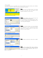
1
Monitoring External Equity Mandates The design of a tool to create exposure graphs for a pension fund M.T. van de Castel Monitoring External Equity Mandates The design of a tool to create exposure graphs for a pension fund University of Twente Enschede, 30 September 2009 Author: Martijn van de Castel Graduation committee: B. Roorda E. Imreizeeq L. Oorthuizen F. el Kanfoudi ~ 2 ~ Management summary At the end of 2008 the equity department of the Grafische Bedrijfsfondsen (GBF) was going to replace the Altis tool that was used to keep track of the way investments were done. Therefore the department was in need of a suitable substitute. This decision of replacement was the starting point of this project. The decision itself is therefore not part of the final assignment which was as follows: Develop a quantitative tool that enables GBF to compare the relevant characteristics of its portfolios with those of their benchmark. Relevant is defined as being both acknowledged by GBF as important and accepted in literature as explanatory. The report is structured around five research questions. The findings will be summarized here together with the corresponding question. In which environment and in what way will the tool be used? The new tool, which will be named RIMOR, will be used solely by the equity department of GBF. Its purpose will be the monitoring of the investments of the portfolio managers. What functionalities should the tool have? The new RIMOR tool needs to be flexible, up-to-date and should produce graphs that compare the characteristics of the portfolio holdings with those of the benchmark holdings. What are the relevant characteristics? Relevant characteristics enable GBF to see whether the investments are in compliance with its guidelines. These guidelines state that the stock portfolio’s characteristics have to match the characteristics of their benchmark as closely as possible and that stock selection should be the primary source of alpha. Carhart’s Four Factor Model is combined with the factors sector and country. The characteristics that are able to depict these factors are Beta, Market Capitalization, country, sector, industry group, Price/Earnings ratio using the Bloomberg next year’s estimated earnings per share and 1 Year total return in percentages To be able to see whether a manager actively manages his portfolio, a module for Active Share is added. What is an efficient way to build the tool? Visual Basic for Excel is chosen as the programming language since it is cheap, easy to maintain and compatible with other applications that are being worked with at the equity department. Because evolutionary prototyping is used as the design method, the users are closely involved in the process. Two kinds of tests are used, chauffeured tests and full user tests. Testing resulted in the addition of a dividend yield and a long term growth indicator. How to familiarize future users with the new tool? To provide new users, now and in the future, with the opportunity to get to know the RIMOR tool a manual is written. This document consists of two main parts. One part explains how to use the tool in daily business and the other explains how it can be altered when requirements change in the future. One person will be in charge of maintaining the tool in the future. A workshop was organized for him where the whole tool and the manual were discussed extensively. The final result is the RIMOR tool. It enables GBF to keep track of the under- and overweights of its investments with respect to preselected indicators that represent important return drivers. The indicators that RIMOR uses can be altered to meet changing needs. By grouping the graphs on one sheet per region or portfolio, a good impression of possible style drifts can be obtained. The addition of the Active Share option completes the spectrum of checks. Together the graphs and the Active Share table enable GBF to monitor the external managers on both angles of the guidelines. ~ 3 ~ In combination with the rest of the available software GBF has access to full range of information on its investments To improve the RIMOR tool even further the following recommendations are made; To keep the indicators up-to-date, the development of new strategies should be closely monitored. Creating an option to select or disable some regions or indicators would improve the tool’s speed. Being able to get historical information would be a major improvement Although there is still room for further improvements it can be concluded that the RIMOR tool is a product that meets all requirements. It has been implemented to the satisfaction of everybody at GBF and it is being used in the daily business processes. ~ 4 ~ Preface To conclude the study Industrial Engineering and Management a final thesis is required. A project done at the Grafische Bedrijfsfondsen, GBF, forms the basis for this report. GBF was in need of a new tool to compare its equity portfolios to the corresponding benchmarks, because the contract with the company that provided this service in the past was about to be terminated. The project consists of three parts which will be described in this report: The Analyses of the old tool Explore the needs and expectations of the users Development and implementation of a new tool The time spent at the equity department was very interesting. Working with the equity team was on the one hand an educational experience. I learnt a lot about investing in general and more specifically about investing at a pension fund. On the other hand it was great to work in such an amicable environment. Next to these things it provided me with the opportunity to experience all the commotion about the credit crisis from inside the financial system which gave me all the information I could never get from the papers and the news alone. At this point I would like to say thanks to some people who helped me to complete my study and especially to write this thesis. First of all, the whole investment team and especially Lambert, Fred, Fouad, Stijn and Jeroen for the educational and above all the pleasant time I have spent at GBF; Roel for helping me find this unexpected place to write my thesis; Dr. Roorda and Mr. Imreizeeq MSc. for all the academic feedback, both on the project and on the thesis. Furthermore I would like to thank Henriëtte and Mrs. Van de Kuinder for reading through the whole document and providing me with feedback. And last but not least I would like to thank my parents for their continuing support, encouragement and love. This thesis is dedicated to them. Enschede, 30 September 2009 Martijn van de Castel To avoid confusion the following remark should be made: where the term “he” is used in this report this can be read as “he” or “she” where appropriate. The same goes for words of a similar meaning like him or his etc. ~ 5 ~ Index 1. Introduction ................................................................................................................................. 7 2. Problem definition....................................................................................................................... 9 2.1. The assignment ............................................................................................................................ 9 2.2. Research questions .................................................................................................................... 10 2.3. Methodology .............................................................................................................................. 10 3. Environment .............................................................................................................................. 13 3.1. Business unit investments ......................................................................................................... 13 3.1.1. Matching portfolio .................................................................................................................... 13 3.1.2. Return portfolio......................................................................................................................... 13 3.2. Equity team ................................................................................................................................ 13 3.2.1. Monitoring the managers ......................................................................................................... 13 3.2.2. Tactical allocation policy .......................................................................................................... 14 3.2.3. The management of the internal mandate .............................................................................. 15 4. Altis............................................................................................................................................. 16 4.1. The functionalities ..................................................................................................................... 16 4.2. What functionalities of Altis can be found elsewhere ............................................................ 17 4.3. What indicators are actually used and which are superfluous ............................................. 17 4.4. Conclusion.................................................................................................................................. 18 5. Creating the framework ........................................................................................................... 19 5.1. Performance .............................................................................................................................. 19 5.2. How to model the portfolio returns ......................................................................................... 22 5.3. How to depict the factors .......................................................................................................... 24 5.3.1. Indicator choice ......................................................................................................................... 24 6. Process ........................................................................................................................................ 28 6.1. Creation of prototype................................................................................................................ 28 6.2. User tests and feedback ............................................................................................................ 29 6.2.1. Chauffeured user tests .............................................................................................................. 29 6.2.2. User manual ............................................................................................................................... 29 6.2.3. Full user tests ............................................................................................................................. 29 6.3. Build final version ..................................................................................................................... 31 6.4. Implementation phase............................................................................................................... 31 7. Conclusion and recommendations ........................................................................................... 33 8. References .................................................................................................................................. 35 Appendix I ............................................................................................................................................ 36 Appendix II .......................................................................................................................................... 37 Appendix III......................................................................................................................................... 39 Appendix IV ......................................................................................................................................... 41 Appendix V .......................................................................................................................................... 42 ~ 6 ~ Introduction 1. “Grafische Bedrijfsfondsen”, GBF, is a foundation that invests and performs administrative duties for the “Pensioenfonds voor de Grafische Bedrijven”, PGB, and other pension funds for the Dutch printing industry. With nine billion Euros of capital under management, it is a midsized fund and a top ten player within the Dutch industry funds. Investing money is a knowledge intensive activity. To do this properly a lot of research is needed. Since it is very expensive to set up and maintain a department to do research or to purchase it from external sources, the equity portion of the capital under management is, for the largest part, outsourced to asset managers. Although outsourcing provides the benefits of a larger research department and in-depth knowledge, it also forces GBF to hand over some of its influence, thus creating an Agency-Principal dilemma. In such a dilemma a way needs to be found for the principal, GBF, to motivate the agent, the external manager, to act just like the principal would have done if he had the same possibilities (Sappington, 1991). GBF needs stable growth of its capital, driven by a set of well diversified investments. On the other hand, the payment scheme of the external managers is composed of a fixed management fee and a variable fee based on outperformance. Because of this, the managers might get tempted to adopt a strategy that is more risky than desirable, hoping to maximize the outperformance and by doing so increase their management fee. This temptation is limited by contracts stating the maximum exposure to certain elements, thus restricting the manager. Another restrictive measure is that the investment style of the external managers is closely monitored. The basis for this is formed by the goals and guidelines laid out in the investment plan (Grafische Bedrijfsfondsen, 2007). The primary goal is to realize beta returns and on top of that the secondary goal is to generate alpha. Alpha is defined as (1) with αp = outperformance of the portfolio, average performance of the portfolio, average performance of the benchmark. GBF uses the basic assumption that its investments should realize an Information Ratio of 0.25 per manager with the idea that this will be 0.5 at a total level. Where (2) and Tracking Error = StDev(RBM – rp) (3) The reason why the Information Ratio on a total level should be higher than on a single portfolio level, is that the average tracking error should be lower. This is the result of diversification benefits between managers while the expected alpha remains the same. The managers should reach the aforementioned goals by means of the following guidelines (Grafische Bedrijfsfondsen, 2007). 1. The stock portfolio’s characteristics have to match the characteristics of their benchmark as closely as possible (Primary objective). 2. Stock selection should be the primary source of alpha (Secondary objective). ~ 7 ~ Until the end of 2008 a computer program was used to support the screening of this process, the Altis tool. Until recently, Altis Investment Management was an independent company1 which has its roots in the multimanager activities of Morgan Stanley. It provides specific services in the sphere of the construction of a manager’s portfolios, risk management, the monitoring of selected managers, bringing forward alternative managers and, with the use of the Altis tool, the quantitative analyses needed to do these things (Grafische Bedrijfsfondsen, 2007). The tool is backward looking; creating reports based on the results of the last month. A Performance Attribution system breaks down performance of a portfolio to show where performance has been made and lost (Altis Investment Management, 2008). In the beginning of 2008 the board of GBF, decided that the contract with Altis would not be extended by the end of 2008. The most important arguments to terminate the contract can be summarized by the following points: the services of Altis are too broad for the needs of GBF, they are too expensive, as a key selling point towards external clients, GBF considers these activities as something that needs to be done in-house. The decision not to extend the contract has a number of consequences especially with respect to the last argument. Since the reason of the cancellation is not that the functions are no longer useful, they will have to be brought in-house. Most of the functions of Altis are taken over by processes already available, like Bloomberg and Dimension, and by the portfolio managers for external mandates. This leaves the quantitative analyses tool to be replaced. Therefore this project has three phases. First research was done to which parts of the Altis tool need to be replaced and which are redundant. Next the needs and expectations of the equity team are gathered and finally the new tool is developed and implemented. This report is organized as follows. In the next chapter the assignment is formalized. This will be done by defining the problem definition, stating research questions and by describing the methodology, which is used throughout this report. The assignment took place at the equity department of the business unit investments. To get a clear picture of the significance of the project it is important to understand the investment process at GBF. Therefore in a short description of the environment will be given in chapter three. The fourth chapter is about the old Altis tool. It will be analyzed, which functions are used in practice and which cannot be replaced by another system that is already in use at the moment. These functions, together with the missing features, form a basis for the new tool. In the fifth chapter a theoretical foundation will be provided. First performance will be defined. Next, literature about portfolio performance will be covered. And the final part will cover the indicators that match the factors found in literature and combines these with the findings of the previous chapter Building on all the information gathered in the previous chapters a description of the final tool’s development can be found in chapter six. Both the development and testing of the tool will be described. Finally in chapter seven conclusions will be drawn and some recommendations will be given. 1 In December 2008 Altis was bought by ING. ~ 8 ~ 2. Problem definition To be certain that everybody has the same starting point, a clear definition of the problem is vital. In this chapter the assignment is formalized. 2.1. The assignment Since all equity portfolios are linked to a benchmark which characteristics, according to the guidelines, should be followed as closely as possible, it is important to know to what extent this is actually done. This needs to be done on different levels. First on an individual portfolio level, secondly on a regional level, both with the same regional benchmark, and thirdly on a total level, where an aggregated benchmark is composed of the weighted averages of the regional benchmarks. Until the end of 2008 Altis provided the tool to visualize the deviations from the benchmark. So, by no longer using the Altis tool, the need for a sound new tool to replace it, arises. This situation resulted in the following initial assignment: Develop a quantitative tool to replace the functionalities of the Altis tool with respect to the comparison of the characteristics of the portfolios to those of their benchmark. Further discussions within GBF resulted in the conclusion that this assignment is too broad to be feasible. The list of different stock characteristics in the Altis tool is too long. Although all these characteristics provide a piece of information on the underlying company it is impossible to control portfolios for all these pieces of information. Therefore restrictions need to be added to the assignment. A selection needs to be made. As Industrial Engineering operates at the intersection of theory and practice, this intersection will be the starting point for the selection. By combining the two angles, literature and practice, a solid basis for the task is formed. In practice fund managers follow a strategy to create value with their investments. Which strategy they choose depends on their ideas of the market movements. Although the number of pursued strategies is limited, fund managers are constantly searching for new ones to create a niche where they can earn money. Since GBF meets with the fund managers frequently they have a good understanding of what is happening in the market. On the other hand, a lot of literature is dedicated to the topic of performance measurement as well. Dependencies are sought between the performance of stocks or portfolios and their benchmark. By refining these dependencies ever further the effects of skill, or stock picking abilities, of managers are reduced more and more. The available knowledge in the two above mentioned fields leads to the following restrictions: 1) The characteristics need to be in line with the perception of GBF of what is important. 2) The characteristics need to be recognized in literature as being explanatory items. In the first restriction, “important” has two components: a) In line with the Investment Management Agreement restrictions formulated by GBF. b) Able to explain sources of non stock specific alpha, not the amount of alpha itself. Taking into account the restrictions mentioned above leads to a new task description; Develop a quantitative tool that enables GBF to compare the relevant characteristics of its portfolios with those of their benchmark. Relevant is defined as being both acknowledged by GBF as important and accepted in literature as explanatory. By making it a quantitative model it is meant to provide the user with insight in the absolute and relative positioning of the portfolios with respect to preselected indicators. This enables GBF to explain the sources of alpha. ~ 9 ~ 2.2. Research questions The task description sets the ultimate goal of the project. In order to reach that goal some questions need to be answered first. These questions will range from general to specific and together the answers will result in the input for the final stage, the building of the actual tool. A project needs to be put into context, so before the actual assignment comes into the picture, a clear idea of the environment needs to be obtained. Who are the users, what is their investment philosophy, how do they work and what will they use the tool for. The next step is to give concrete form to the tool’s expected capabilities. A good starting point for this question is the old tool. The set of functionalities needs to be analyzed, since some of them will be needed in the new tool and others will not be used anymore in the future. Next to this it can be very well possible that some new functionalities will have to be added. These can be found by consulting the people at GBF. Answering the main question by means of the sub questions, the expectations with respect to the tool’s requirements are mapped out. Once the framework is set out, the finer lines need to be filled in as well. Characteristics need to be determined. The problem with the first task description is that it is impossible to use all thinkable characteristics. Therefore the characteristics that are needed will have to be determined. By taking both the theoretical and the practical angle an optimal mix is obtained. So the question ‘What are the relevant characteristics?’ has to be split into two sub questions, namely ‘what are the important factors according to GBF?’ and ‘what are important characteristics according to literature?’. So far all the answers will provide a list of the requirements and abilities for the tool. The next step will be the actual build of the tool. To do this as efficiently as possible a way of construction is needed which enables the users to provide feedback and in this way the user has influence over the final design. In short the question is ‘what is an efficient way to build the tool?’. Finally the tool has to be used when it is finished. Since the tool is a permanent solution which will be integrated in the daily business, the users will need to know how to use the tool. The final question that needs answering is therefore ‘How to familiarize future users with the new tool?’. A. In which environment and in what way will the tool be used? B. What functionalities should the tool have? a. What functionalities of the old tool have to be incorporated in the new tool? b. What functionalities are missing at the moment? C. What are the relevant characteristics? a. What are the important factors according to GBF? b. What are important characteristics according to literature? D. What is an efficient way to build the tool? E. How to familiarize future users with the new tool? Text Box 1. Summary of the research questions 2.3. Methodology The questions above are very diverse but have to be taken together to produce coherent result in the end. The diversity of the questions also demands diversity in the way these questions are approached. Below the different techniques which were used during the project are being dealt with. Where and in what way will the tool be used A lot of information on the structure and the way of working of the investment unit is documented within the company. This is a valuable source of information. One especially useful document is the investment plan. In this document the different departments of the investment unit are described together with their targets, expectations and market views. To get a clear description of the way GBF invests its money this document is used. Further documents which served as background information were the reports for the monthly investment policy team meetings. Next to the documentation available other important sources of information were attending the meetings with external managers, the meetings of the investment policy committee and the meetings of the equity team. ~ 10 ~ What functionalities should the tool have To be able to answer this question the abilities of the old tool were examined and discussed with the users. By interviewing these users, it became clear which parts of the program were actually used and which parts were redundant. Since building a new tool also provides the opportunity to enter new possibilities, the users were asked what extra functionalities should be incorporated in the new tool. Also, Altis was compared to the other programs already in use at GBF to determine what functionalities were overlapping and therefore would not be needed in the new tool. What are the relevant characteristics Once the functionalities of the new tool are established, it needs to be determined what the new tool actually will have to measure. To make sure that the project has both a theoretical and a practical basis the choice is made to take these two angles as the starting point. For the theoretical basis literature on the explanation of portfolio returns is studied and for the practical basis interviews with users were combined with information obtained during the various meetings. What is an efficient way to build a tool To keep the tool user friendly and at low cost, the choice has been made to use Microsoft Excel as a basis. Excel is convenient since it is already installed on every user’s computer and it can be linked to the Bloomberg terminals of the equity department. This link enables easy access to up-to-date information. An extra advantage is that the output can be processed easily in other standard applications as well. Next to this, it is equipped with a very intuitive programming language, Visual Basic for Excel (VBA). VBA is relatively easy to learn, which is especially important since it makes it easy for others to make adjustments to the tool in a later stage. A disadvantage of VBA is its speed, since it is a relatively slow language. This weakness is definitely relevant since the tool will have to process large amounts of data. All in all, the advantages in combination with the fact that the tool will only be used about once a day instead of on an ongoing basis, outweigh the speed of the language. Next to the basis for the tool, the process used to build the tool is equally important. To benefit from user input as much as possible it is a necessity to consult users frequently. The input obtained in this way will provide the basis for further improvements. Not only does this way of working speed up the process, it also enhances the acceptance of the end product. In order for this process to work, it must be easy to alter the original design and to implement the proposed changes. A process which is very suitable for these criteria is evolutionary prototyping. Evolutionary prototyping is the design of an incomplete but highly flexible system, followed by the sequence of creation, testing, and re-design which is repeated several times. Each pass through the cycle should entail small changes as new features are added, until finally all requirements are met (Minka, 2005). In different stages of the project different ways of testing can be used. Here, for the first tests chauffeured prototyping was used. This means that demonstrations of the tool’s abilities were given. The user does not actively participate in the demonstration, but instead comments on what he sees. These comments are then used in the next phase of the development. The next step was using a full prototype which is actively tested by the users. This step is extremely useful since the tool is used by someone who is not biased by in-depth knowledge of the program. In this way logical errors come to light and things that are unclear will be brought up. Finally the tool faces up to its expectations and comes into use. In time new user demands will arise and the process starts over. Independent of the way of testing, the same cycle of steps needs to be passed through (Georgia Tech College of Computing, n.d.). A schematic overview of this process is given in figure 1. ~ 11 ~ Figure 1. Design cycle. How to familiarize future users with the new tool Both during the prototyping cycle and afterwards, the users have to understand the way the tool functions to be able to work with it. There are several ways to familiarize people with a new product. This ranges from learning by doing, to a step by step walkthrough by an instructor. For this project two approaches are chosen. Since one person is appointed to develop the tool further once the project is finished, a workshop with a step by step explanation of the tool and underlying code is organized. Although this is a very time consuming process, it provides the user with the thorough understanding of the tool’s layout and functionalities. For the other users a manual is created explaining all functionalities, the layout of the tool and the way to perform some basic alterations in the future, like adding and removing indicators. Since a manual is a lasting document it can be used to familiarize future users with the tool as well. ~ 12 ~ 3. Environment As stated, the assignment took place at the equity department of the business unit investments. To get a clear picture of the significance of the project it is important to understand the investment process at GBF. Therefore in this part of the paper a short description of the environment is given. 3.1. Business unit investments For 2009, GBF’s total assets are divided in 35% equity, 44% fixed income, 20% real estate and alternative investments and 1% cash. Real estate and alternative investments is subdivided in 10% real estate, 5% infrastructure, 2.5% commodities and 2.5% hedge funds. During a weekly meeting the department heads keep each other up-to-date. The asset classes are placed in a matching portfolio or a return portfolio. Each of them has a specific goal. 3.1.1. Matching portfolio The portfolio is used to reduce the influence of fluctuation in the interest rate and inflation on the coverage ratio. For this purpose it tracks the development of the Provision Pension Liabilities, the PPL2. The PPL is a technical provision based on the accrued pension rights of the pension funds participants (De Nederlandse Bank, 2007). The cash flow of the liabilities valued against the swap rate is taken as the benchmark for the matching portfolio. The inflation and interest rates have the biggest impact on the PPL, therefore the matching portfolio partially hedges against these characteristics (Grafische Bedrijfsfondsen, 2008). The matching portfolio has to be considered in combination with the liquidity portfolio due to the similarity in characteristics. Therefore it is complicated to define the exact impact of the portfolio on its own. Given that the matching portfolio has no direct implications for the tool, we will suffice with mentioning its existence and main goals here. 3.1.2. Return portfolio Next to the matching portfolio, a return portfolio is constructed. The primary goal of this portfolio is to generate extra return to cover the costs of the inflation and interest coverage in the matching portfolio. The secondary goal is to create excess return. In this way the reserves are filled, which are used to deal with actuarial risks and to keep the contributions of the participants as low as possible. 3.2. Equity team The asset class equity is located in the Return Portfolio. The activities of the equity team can be divided into three core tasks: 1. monitoring the managers, 2. the tactical allocation policy, 3. the management of the internal mandate. 3.2.1. Monitoring the managers For a good diversification of the portfolio the equity funds are split-up into nineteen portfolios which are spread over six regions, North America, Europe ex UK, UK, Pacific ex Japan, Japan and Emerging Markets. Each region and their related portfolios have the corresponding MSCI IMI region index as their benchmark, MSCI US IMI, MSCI Europe ex UK IMI, MSCI UK IMI, MSCI Pacific ex Japan IMI, MSCI Japan IMI and the MSCI Emerging Markets IMI respectively. Eighteen of the portfolios are managed externally, five of which, the ones printed in italics, are participations in investment funds, the other thirteen are handled by asset managers. The target of the portfolios is to generate both beta returns and outperformance with respect to their benchmark, alpha. As mentioned in the Introduction, the objective is to have an Information Ratio of at least 0.25 per manager and an overall information ratio of 0.5 due to diversification effects. 2 In Dutch: Voorziening Pensioen Verplichtingen (VPV) ~ 13 ~ The thirteen mandates mentioned are subject to an Investment Management Agreement, IMA. These contracts embody all the conditions, such as the target return, portfolio size and the benchmark and all the limitations, like maximum sector deviations and the tracking error. Next to that the fee structure is included; usually this fee consists of a fixed management fee and a performance fee. The IMA’s function is twofold. On the one hand a manager’s performance can be measured and evaluated and on the other it diminishes the negative effects of outsourcing described earlier. Since the external mandates are managed individually by managers from different companies, the managers have no information about the other mandates. Therefore one of the core tasks of the equity team is the monitoring of the asset managers. Monitoring is about keeping track of the exposures caused by manager’s positioning and thus being able to explain the manager’s performance. In this perspective, the different levels of aggregation are of great importance too, since intervening can only be done sensibly on an aggregate level, be it regional or total. Intervening per mandate could lead to similar transactions in the opposite direction, which is a waste of money. Monitoring is meant to detect style drifts and is not a check whether or not the manager stays within the limits of the IMA. This verification is performed by the Finance and Control department. Before the project, the team had three kinds of methods at its disposal to monitor the managers; Dimension Manager reports, visits, conference calls etc. Altis Dimension is an investment administration system. All positions are stored in this system and because of this it is possible to examine the performance of both separate and aggregated mandates. The Altis tool is an instrument used to do quantitative analyses (Grafische Bedrijfsfondsen, 2007). The analyses are important because they provide insight in the positioning of the investments. This is helpful in explaining the sources of performance. The tool will be further discussed in chapter four. 3.2.2. Tactical allocation policy The tactical allocation is also one of the core tasks and can be divided into three categories: 1. Tactical allocation to the equity bucket, 2. Tactical allocation to the regions within the equity bucket, 3. Tactical allocation to currencies within the equity bucket. Tactical allocation to the equity bucket As stated in paragraph 3.1 the equity bucket is only part of the spectrum of investment products. Once every six months, the under- or overweighting of the equity class is created. In this case, under- or overweighting means, taking a smaller or larger share of equity in the total portfolio of investments than decided upon in the investment plan. The rebalancing is done by means of listed futures, this will be explained below. Usually the weight is changed in comparison with the fixed income bucket. Since this is done on PGB level, it is important that these actions are discussed with the other departments; this is done during the weekly meeting of the department heads and/or the monthly meeting of the Investments Policy team. The Policy team consists of all the people of the business unit investments and one person from the risk management department. Tactical allocation to the regions within the equity bucket Next to the under and overweighting on a PGB level, it is also done on a regional level. Normally this is done with futures, except for the cases where this will not work well enough. In that case money could be taken away from or given to the managers. As can be seen in Appendix I table 2 a range of plus or minus 30% deviation from the norm has been set. This leaves room for acting on short term views. Generating extra performance and/or reducing risks are the main objectives in this case. ~ 14 ~ Tactical allocation to currencies within the equity bucket The tactical currency allocation is done with forward contracts. The possibilities are limited because the maximum currency exposure at PGB level is set to 10%. The currency hedging is done on PGB level because, as with positional hedging mentioned in subsection 3.2.1, it should not be done by the individual managers themselves. After all they do not know the other positions and that could lead to double hedging and unnecessary expenditures, too. As mentioned, the rebalancing is done by means of futures and forward contracts. This has a simple explanation. When a bucket is rebalanced, exposure has to be bought or sold. One way to do this is to buy or sell the actual stocks. The advantage of this approach, is that exposure can be adjusted very precisely. The biggest disadvantage is that buying single stock positions is a very expensive and labour-intensive approach. The other way is to buy futures or forward contracts on an index. This has the big advantage that these contracts have a high liquidity and that they provide a cheap way to create or reduce exposure. 3.2.3. The management of the internal mandate One person is responsible for the management of the internal mandate. This is done by using a quantitative model which is developed in-house at GBF. To optimize the Information Ratio the model uses broker advices combined with a series of restrictions, such as the maximum under- and overweight in single stocks, being sector and market capitalization neutral etc. The portfolio is rebalanced every six weeks and kept static in between the rebalance points. To be able to profit from market movement in the meantime, stock options are traded. ~ 15 ~ 4. Altis The reason that the Altis tool has been abandoned, is not that it does not work, but that it is too expensive and too broad and because it is an outside product. Therefore, it is sensible to take a look at its possibilities before creating a new one. In this chapter this will be discussed in more detail. Then a selection will be made of the functionalities the new tool will need. 4.1. The functionalities The Altis tool provides a quantitative overview of how a portfolio has been composed and what the contribution of this composition was to the performance. In this process it is assumed that the positions have not changed during that month. The composition of the portfolio at the beginning of the month is taken as fixed. The overviews are therefore static and have to be reinstalled after every update. The file becomes available approximately two weeks into the new month, resulting in a maximum time lag of six weeks. Figure 2. Time lag Altis depends on the external managers for the file’s input. They provide the names and the quantities of the stocks they hold in their portfolio each month. By gathering information on the characteristics of these positions reports can be made in which the performance and constitution per item can be depicted. These quantitative reports can be made on a large number of characteristics or indicators, like the net income of a company, the home country or the average daily volume. A complete list of the indicators and their corresponding factor and scale can be found in Appendix II. The output that Altis provides is a file that shows three graphs on the selected indicator and a table containing the data of the graphs plus two columns with the allocation and the stock picking effects. In the first two graphs, the absolute weights and the performance of both the benchmark and the portfolio are shown and in the third graph the alpha distribution and the corresponding relative weight is depicted. So effectively the third graph displays the difference of the bars of the first two graphs, relative weight for the first graph and alpha for the second one. For each of the 76 indicators these graphs can be created. Below an example is shown where the indicator “GICS Sector” 3 is used. This output is static which means that though the indicator which is depicted by the graph can be changed, the data available for that indicator is always the same and the scale of the graphs is unchangeable as well. In the new tool both the bucket size and the holdings have to be flexible so they can be adjusted by GBF whenever this is desired. In Appendix V the user manual for the tool can be found. In Part 1 of the manual it is explained how these things can be done (respectively on page 9 and page 1–7 of the manual) and in Part 2 an explanation of the code behind the process is provided. The changing of the portfolios is discussed on the pages 14-16, 20 and 22. 3 GICS (Global Industry Classification Standard) is an industry classification standard developed by Morgan Stanley Capital International (MSCI) in collaboration with Standard and Poors (S&P). The Global Industry Classification Standard consists of 10 sectors, 24 industry groups, 62 industries, and 132 sub-industries. The GICS classification assigns a sector code to each company according to its principal business activity. (Bloomberg, 2009) ~ 16 ~ Figure 3. Altis report. Graph 1: the absolute weights of the portfolio and the benchmark. Graph 2: the performance of the benchmark and of the portfolio. Graph 3: the alpha distribution and the corresponding relative weight. Tables: data of the graphs, columns with the allocation and stock picking effects and the contribution. 4.2. What functionalities of Altis can be found elsewhere In subsection 4.1 the functionalities of the Altis tool are shown. Information is provided about the absolute weights and the performance of the portfolios and the benchmarks, the alpha distribution and the portfolios relative weight. Not all of this information is needed from the tool since other application can provide it as well. Dimension stores the positions of every portfolio and provides GBF with their performance. This information can be obtained from the second graph of the Altis tool as well. Therefore this feature does not have to be included in the new tool. Since the third graph is created from subtracting the portfolio values of graph one and two from the corresponding benchmark data this graph does not present new information as well, which leaves the first graph to be reconstructed. On page 8 of the manual in Appendix it is explained how this can be done and on pages 17-20, 21 and 23 an indebt description of the process is given. It was decided by GBF that the data presented in the tables did not have to be included in the new tool. 4.3. What indicators are actually used and which are superfluous On their own all the indicators of Altis seem to be useful. But useful does not mean indispensable or even needed. In fact, the availability of too many functions compromises the usability of the tool. Therefore it is important to know which factors are used frequently, which are used sometimes and which can be left out since they are never used. Interviewing the users is a good way to obtain this information. In this way hands-on information can be gathered and a custom build tool can be developed. Two categories of indicators can be distinguished, 1) Used often, 2) Seldom or never used. ~ 17 ~ The indicators marked as used often, will be taken as the indicators suggested by GBF. The number of available indicators is so large, that in practice the biggest part of the indicators is not used at all. The survey learned that only 15 indicators, or 19.7% of the available 76, are used on a regular basis. In alphabetic order: Beta (Market), Dividend Yield (set of 2) (Value/Growth), Earnings per Share (set of 3) (Value/Growth), Market Capitalization (Size), Momentum (Momentum), Operating Margin (Other; Profitability), Price Earnings (set of 3) (Value/Growth), Price to Cash flow (Value/Growth), Return on Equity (Other; Profitability) and Sector (Sector). The categorization of these indicators per factor can be found in Appendix I table 3. In section 5.3 the final choice of the indicators will be presented. In that section the availability of the indicators will be tested as well. The flexibility mentioned in section 4.1 also applies here. It should be possible to add new indicators in the future. How this can be done is explained in detail on pages 24-31 of the manual in Appendix V. One could conclude, that the figures that are used are basic key figures which are widely available on a single stock level. However, it should be kept in mind that the purpose of the tool is to provide GBF with an overview of its positions on a more aggregate level, namely on a portfolio, a regional and a total level. This was exactly the function of the Altis tool. It provides an overview of the sum of the weights of assets which fall in a predefined bucket. To do this, it processes thousands of positions and a multiple amount of data points, which is impossible to do by hand. 4.4. Conclusion The analysis of the Altis tool resulted in a list of functionalities and indicators that could be used for the new tool. This list will be summarized in this paragraph. The information that should be provided is a graphical depiction of the way the different portfolios and regions are spread over the indicators. The indicators used often in the Altis tool are taken as the first indicators recommended by GBF. These are: Beta, Dividend Yield (set of 2), Earnings per Share (set of 3), Market Capitalization, Momentum, Operating Margin, Price Earnings (set of 3), Price to Cash flow, Return on Equity and Sector. From another angle, the new tool should also be more flexible with respect to the refreshing of the holdings, the changes in the indicators and the alteration of the bucket sizes. In other words it should be able to adjust the tool to specific needs over time. ~ 18 ~ 5. Creating the framework To provide GBF with a robust tool, a theoretical foundation will be provided in this chapter. Since the largest part of the funds that are allocated to the equity department is outsourced to external managers, it is no more than logical that there is the need to know where the performance of these managers originates from. To be able to do this it is important to define performance first. The second part of the chapter covers literature about portfolio performance. The final part covers the indicators that match the factors found in literature and combines these with the findings of the previous chapter. 5.1. Performance Two ways to define performance which are often used in practice are absolute and relative performance. Absolute means that performance is the actual change of the portfolio’s value and relative performance is the difference between the absolute performance of the chosen benchmark and that of the portfolio. This either results in outperformance, a positive outcome, or underperformance, a negative outcome4. The two ways of performance measurement are closely related since the relative performance of a fund is the difference between its own absolute performance and the absolute performance of the benchmark. The most desirable outcome is both a positive relative performance and a positive absolute performance since in that case, the investment is not only making money; it also makes more money than its benchmark. The opposite situation, both a relative and an absolute under performance is the most unattractive scenario. In between is a grey area. The upper left corner represents a situation where the benchmark is outperformed, but where the value of the investment still shrinks. A situation where this is likely to occur is an overall downward movement of the markets like in 2008. The lower right corner is a situation where the investment makes money but where the benchmark performs better. This can happen with a portfolio which is too defensive in an up going market. Which of the two is more desirable, depends on your view on investing. A pension fund is interested in absolute performance, whereas a manager, who is paid for the amount of alpha that is generated, will prefer the relative performance. Figure 4. Absolute versus Relative return The two different ways of measurement both have their own implications. When performance is measured in a relative way, portfolios usually get constraints forcing them to stay close to the selected benchmark and generate the desired outperformance by means of stock selection, instead of major bets on, for example, one or two sectors. Underlying is the link between risk and return; without the constraints, the portfolio manager might be tempted to follow a very risky strategy. In that case the return potential is high, but so are the risks of a potential loss. Although the same theory applies to an absolute return portfolio, looser constraints are needed in order to make a positive performance possible even when the market shows a downward trend. For example the use of unconventional assets, short-selling, options, futures and other derivative strategies and leverage can be used (Investopedia.com, n.d.). Besides good constrains the chosen benchmark has to be good and relevant. For a benchmark to be good and relevant it has to fulfil the six widely-cited criteria which are shown in text box 2 (Guarino, 2008). 4 NB: This is independent of the absolute performance, a negative return can be outperformance and vice versa. ~ 19 ~ “In making its determination, Standard & Poor’s points to six widely-cited, key principles of a good, relevant benchmark1: Unambiguous: The names and weights of securities constituting the benchmark are clearly delineated. Investable: The option is available to forgo active management and simply hold the benchmark. Measurable: The benchmark's return can be calculated on a reasonably frequent basis. Appropriate: The benchmark is consistent with the manager's style. Reflective of current investment opinions: The manager has current investment knowledge (be it positive, negative, or neutral) of the securities that make up the benchmark. Specified in advance: The benchmark is constructed prior to the start of an evaluation period.” […] 1) (Bailey, 1992) Text Box 2. Benchmark criteria Most pension funds adopt a relative performance strategy. This has several reasons; firstly, pension funds invest for a long period of time, leaving room for some downward movement along the way. In an ideal situation the negative effects of a benchmark that goes down are reduced by outperforming that benchmark, while the positive impact of an upward market is enlarged by outperforming that market as well. Secondly, growth of the principle amount is needed. It is very hard to generate the growth needed with an absolute return strategy by pure alpha alone, that is, alpha, generated solely through stock selection, without taking big risks. This is due to the efficiency of the markets, which leaves the risk premium of the assets as the main source of growth. As mentioned before, to be able to generate performance in markets with a downward trend some form of short selling has to be allowed, this automatically leads to summing away the risk premium of the stocks. To make it possible to fairly calculate the relative performance of a manager, it is very important that the benchmark provided matches the style of the manager’s mandate. The 4th point about benchmarks defines “appropriate” as “consistent with the manager’s style”; however this point is rather trivial within the context of this report. Since every region has a fixed benchmark it is not the benchmark that has to be consistent with the manager’s style, it is the other way around. A manager that invests in Japan must have a style that is in line with the MSCI Japan IMI. Nevertheless, it is possible that managers change their strategy over time. Because of this it should be checked whether a manager still follows the benchmark, or that he is creating value by following a different strategy, thus altering his risk profile. Following the logic of the 4th criterion, the benchmark should be changed when this would happen. In this case the manager will be the one who has to change since the benchmark is fixed and reflects the investment philosophy of GBF. ~ 20 ~ Figure 5. Breakdown of MSCI Indices. Source: MSCI Presentation. To be able to select the right benchmark, it is essential to know the strategic view of the pension fund. For example does it believe in strong sector bets, a value strategy, or momentum trading? When the strategy of choice is a value strategy, it is logical to measure a manager’s performance against a value benchmark as well. GBF believes in a core strategy divided by region. A core strategy means that investments are made in all types of stocks without favouring, among others, value, growth, small cap or large cap stocks and without momentum trading. In other words a well diversified broad market portfolio is created. Which makes up for 98% of the market equity investable universe, as can be seen in figure 5. Next to the core strategy the world is divided into the six regions already mentioned in subsection 3.2.1. The benchmark representing this strategy is a regional Investable Market Index, a combination of the Small, Mid and Large Cap Indices. By using the predefined IMI index all of the six conditions for a good benchmark are met as is summarized in Text box 3. Unambiguous: The underlying assets can be accessed and the turnover is low. Investable: The MSCI indices only contain liquid stocks. Measurable: The indices are quoted on an ongoing basis. Appropriate: A Core Strategy is adopted; an investable market index is a good match with this strategy since it represents an investment in a broad market portfolio. Reflective of current investment opinions: Since the market indices are regional, and linked to the region in which the manager operates, he should have an opinion on the assets of the benchmark. Specified in advance: All the indices already exist for at least ten years with starting dates ranging from 1969 to 1998. Text Box 3. Benchmark characteristics. Since the performance of the managers should be based on beta returns increased with as much alpha as possible5, the payment is based on that assumption as well. To make sure managers stick to their 5 While staying within the restrictions or guidelines as outlined in the IMA. ~ 21 ~ mandate and do not create false alpha by pursuing other, riskier, strategies, their activities have to be monitored. First a suitable way to depict these possible exposures is needed. As mentioned, before this was done by the Altis tool. 5.2. How to model the portfolio returns According to Conner and Korajczyk, a characteristics-based model is a good way to factor model security returns. The factor betas of an asset are tied to observable characteristics of the securities, such as company size or the book-to-price ratio, or the industry categories to which each security belongs (Connor & Korajczyk, 2007). Although the goal of this project is to create a tool that provides the user with an intuitive overview of a portfolio’s composition, rather than with a statistical listing of the covariances between the portfolio and the factors, factor modelling can form a good starting point. The reason for this is that it points out what the important return drivers, or factors, are. Over the past decades several models have been developed and expanded. A selection of these models will be discussed in this paper. They will provide the theoretical basis for the tool. Figure 6. Time line, CAPM One of the basic methods of modelling returns is Sharpe’s Capital Asset Pricing Model (Sharpe, 1964) where the β is used to link the expected rate of return of the portfolio to the expected rate of return of the market portfolio. Thus β is the covariance of the portfolio with the market. The idea behind this model is that a company is exposed to two types of risk. These types are systematic risk, which is correlated to the market and cannot be diversified away and non systematic risk, which is uncorrelated with the market and can be diversified away. Since uncorrelated risk can be diversified away it does not need to be rewarded. For the correlated risk on the other hand the investor has to be paid a risk premium. Rt - RFt =α + β(RMt - RFt) + εt With E[εt] = 0 Where Rt = RFt = RMt = α (4) Portfolio return at time t, Risk Free return at time t, Market Portfolio return at time t, should be 0 for all assets. Although the Capital Asset Pricing Model is intuitive and relatively easy to implement and understand, there are some arguments against it which are covered, among others, by Fama and French (Fama & French, 2004). The market portfolio, the returns and the beta are hard to identify and the outcome of empirical evidence is mixed. Several alternatives are proposed, for example the Multifactor CAPM or the Arbitrage Pricing Theory Figure 7. Time line, APT In his paper Ross (Ross, 1976) shows an alternative asset pricing model. The one factor CAPM formula is expanded to a multifactor model, where each factor represents a return driver. By not naming these return drivers specifically, a model is created that covers all drivers that influence the ~ 22 ~ return thus explaining it completely. At the same time, this is the big weakness of the model. By not naming the return drivers, the model just provides a way of thinking, without much practical use in this case. Figure 8. Time line, 3-Factor Model Later, Fama and French (Fama & French, 1993) demonstrated that the factors value versus growth (HML) and company size (SMB) have great influence on the portfolio’s performance. Since these factors are not taken into account by the CAPM model, they are named anomalies. By extending the CAPM formula with value versus growth and small market capitalization versus large market capitalization, better known as the Three Factor Model, the explanatory power of the model was drastically improved. Rt – RFt = α + β(RMt - RFt) + γ(SMBt) + δ(HMLt) + εt With E[εt] = 0 (5) Where SMBt = HMLt = the return of a portfolio of small stocks minus the return of a portfolio of big stocks with respect to market size, the return of a portfolio of high book-to-market stocks minus the return of a portfolio of low book-to-market stocks. Figure 9. Time line, 4-Factor Model As a fourth dimension, Carhart (Carhart, 1997) added momentum to the Three Factor model, depicted as the one year momentum in stock returns (PR1YR), thus creating the Four Factor Model. A year earlier momentum was already mentioned as an anomaly by Fama and French (Fama & French, 1996). Note that Carhart’s model is purely meant to provide an explanation for the returns rather than a specific overview of the risks involved. Rt – RFt = α + β(RMt - RFt) + γ(SMBt) + δ(HMLt) + θ(PR1YRt) + εt With E[εt] = 0 (6) Where PR1YRt = difference between the high and low prior return portfolios. Figure 10. Time line, Country and Sector Hamelink, Harasty and Hillion (Hamelink, Harasty, & Hillion, 2001) show in their paper that there are two more factor besides those already mentioned which have a strong influence on equity returns. ~ 23 ~ These factors are country and sector effects. In their paper they argue that the importance of the factors size and value/growth are not compromised by taking in country and sector effects and therefore they are a valuable addition to the spectrum6.7 The theory shown above provides a set of widely used factors for the portfolio structures and consequently it shows to what extent the portfolios follow the structure of the benchmark. In this manner the primary objective of the guidelines, the stock portfolio’s characteristics have to match the characteristics of their benchmark as closely as possible, can be checked. However, the second one, stock selection should be the primary source of alpha, cannot be reviewed with these indicators. Although all managers claim to be active managers it remains to be seen whether this is true or not and if so, to what extent. To be able to measure how active managers really are, Active Share was introduced (Cremers & Petajisto, 2007). Active Share expresses the part of the portfolio holdings that differs from the benchmark’s holdings. In their paper Cremer and Petajisto assume that mutual funds do not short sell stocks. This assumption is in line with the policy of GBF. For such a long-only portfolio the active share will range from zero to a hundred percent, where zero means an exact replica of the benchmark, and one hundred means that all the stocks in the portfolio are non benchmark stocks. When short selling is allowed, the Active Share can rise above one hundred percent significantly. ∑ , (7) , Where wfund, i = windex, i = the portfolio weight of asset i in the fund, the portfolio weight of asset i in the index. 5.3. How to depict the factors Not all of the factors are usable as such, because some are generic terms for a category. For these factors additional indicators need to be found. Subsequently the availability of these indicators needs to be checked to make sure they are usable. For clarity, in the text below the main categories like value, growth and momentum are called factors and their characteristics, like price to cash flow, dividend yield and beta, will be called indicators. 5.3.1. Indicator choice The number of different indicators that are available and needed differs per factor. Especially for value versus growth multiple indicators are available. To be able to create a meaningful model that is applicable to portfolios regardless of their regional focus it is important to know that the selected indicators are widely available. A logical way to test this, is to take a large, representative pool of equity and see what percentage of the selected data is available. Because the nineteen portfolios are spread over the six regions which together span the whole world, a world index is a suitable choice. The big advantage of a pre-constructed index is that weights are addressed to the positions. In this way the impact of a company is related to its size in the 6 In the paper sector and country are compared to the three factor model so momentum is not taken into account although it is mentioned that in contrast to country the factor sector is sensitive to momentum. 7 Cremers, Petajisto and Zitzewitz (Cremers, Petajisto, & Zitzewitz, work-in-progress, 2008) show that both the three and the four factor model have a serious bias with respect to the alpha predicted by these models. These biases are caused by the way the stocks are grouped. The market capitalization in the big size and low book to market segment is significantly bigger than in the small size and high book to market segment. In combination with the equal-weighting of the segments this leads to an overweighting of the small size and high book to market segment. Although the outcomes of the models are biased because of the factor distribution, the factors themselves are not under dispute. Therefore the factors of the four factor model in combination with the two factors mentioned by Hamelink et al. seem to form a good starting point for creating the tool. ~ 24 ~ index. Although there are several world indices8 the constituents are not available for all of them. Only the constituents of the MSCI All Country World Index, 2439 members, and the Bloomberg World Index, 48349 members, are accessible at GBF. Although the MSCI indices are considered to be the standard, the number of constituents of the Bloomberg Index outweighs the MSCI’s reputation. This is because the main purpose of the index test is to check whether or not the indicators are widely available. To be used indicators have to have 95% availability, the results are shown in Table 4 of Appendix I. Market indicators Most factors have separate indicators, the market factor does not. It is generally represented by its multiplier, beta. With an availability of 96.02% the β of most stocks is available via Bloomberg10 where it is defined as: “Beta estimates the degree a stock's price will fluctuate based on a given movement in the representative market index”. As the representative market index the assigned benchmark is taken. Market capitalization indicators The only indicator applicable to this factor is market capitalization itself where it is defined as: The current total value of all outstanding shares in the pricing currency. The value is converted to Euros. This indicator has an availability of 99.02%. Values versus growth indicators For the value growth factor a large set of indicators is available. Since value stocks are defined as stocks trading at a low price with respect to their fundamentals, in principle all these fundamentals come into the picture as possible indicators. In literature there are indicators which are mentioned on a repetitive basis, these are book-to-market equity, earnings price and cash flow to price. For their Three Factor Model, Fama and French (Fama & French, 1993) tested several indicators, namely leverage, Earnings/Price and Book to Market Equity. When taken into account separately, all of these indicators have positive explanatory power. On the other hand, when the indicators are combined, book to market equity absorbs the other indicators. So in literature book to market equity is seen as the indicator to use. In Bloomberg this indicator is not readily available, but it is easy to calculate because is there which is equal to . With an availability of 98.92% it is a usable indicator. On the other hand GBF believes that the book to market equity indicator has the big disadvantage of being a slow indicator. The book value of a company only changes slowly over time and is more vulnerable to the company’s specific way of accounting. Therefore it is better to take an indicator that gets its input from the “top” of the profit and loss statement. The first one that comes to mind is the price to cash flow ratio. The problem with this one is that it is only available for 70.04% of the sample. The price earnings ratio (PE) has an availability of 95.53% and as a result is therefore the first one that is useful. However the PE uses the current price over the past earnings, which results in an outcome that is skewed. Since the expected earnings are already counted into the current price, the estimated PE is a better indicator because it provides a more forward looking result. For the forward PE there are two options, either the current years PE or the next year’s PE. The problem with both standard PE estimates is their availability, 92.45% and 88.22% respectively. A good substituted is formed by the Bloomberg estimated PE, or BEst PE, which has an availability of 95.84% and 97.20% respectively. Taking into account the comments on the PE ratio and the availability, the Bloomberg Estimated Next Year’s PE seems to be the most suitable choice. Its official definition is: The company’s price/earnings ratio using the BEst next year estimated earnings per share. 8 Dow Jones World Stock index, FTSE World Index, MSCI All Country World Index and Bloomberg World Index are the ones found in Bloomberg. 9 As of 23 January 2009 10 All indicator definitions are obtained from the definition list of the Bloomberg Excel Add-In (Bloomberg, 2009) ~ 25 ~ Momentum indicators Two indicators mentioned are the relative strength index and the past returns. The relative strength index is a technical analysis indicator which measures the magnitude of gains over a given time period against the magnitude of losses over that period (Investorwords.com, n.d.). When the relative strength index has a value of 30 or lower, a stock is considered to be oversold whereas a value of 70 or higher indicates an overbought condition (WebFinance, Inc., n.d.). The big advantage of this method is that it gives a single number with a clear interpretation. The disadvantage is that the maximum number of days considered is 30 which makes it impossible to get a long term picture. Momentum based on past returns is the one most referred to in literature. Depending on the time frame momentum is a predictor of the direction of price movements. The timeline is split into three parts, the very short term, a week to a month, the medium term, 3 to 12 months, and long term, 3 to 5 years, where both short and long term trends tend to reverse during the next period (De Bondt & Thaler, 1985) and a medium term movements indicates another period of that direction (Scowcroft & Sefton, 2003). Bloomberg provides the one year total return in percentage which has an availability of 98.94%. Other indicators As with market capitalization the country and sector factors are indicated by themselves. Since the aim of the portfolio managers is to track the benchmarks as closely as possible, segmentation into ten sectors is rather broad. So it is suggested that an extra factor, the ‘GICS industry group’ consisting of 24 categories (MSCI Barra, 2008) will be added to refine the portfolios a bit further and to gain better insight in the portfolio’s composition. Although this refinement could go up to two layers deeper this would compromise the readability of the reports since it would split into 67 or even 147 categories. All of these indicators are widely available with 99.97% for country and 99.82% for both sector and industry group. By combining all the above mentioned indicators the tool takes advantage of the mixture of fundamental and technical analyses thus providing a wide view on the portfolio composition. To summarize the following indicators are chosen to be used: Beta Country GICS Sector GICS Industry Group Market capitalization Price/Earnings ratio using the BEst next year’s estimated earnings per share 1 Year total return in percentages A complete list of the definitions as provided by Bloomberg can be found in Appendix III. Active Share In contradiction to the indicators, Active Share cannot be depicted with a graph. It is a single number for each portfolio. By composing a table the user is able to compare the various managers in one view and get an idea of how active the portfolio managers are. Next to the active share a calculated weight is added to the table to see what percentage of the total region is covered by one manager. The weights can be very useful to estimate the impact of a portfolio, especially with respect to the other indicators11. A more detailed description of how Active Share is included in the new tool can be found on page 17 of the manual in Appendix V. A word of caution is appropriate. To be able to draw valid conclusions from the results, they have to be persistent. All results are snapshots of the situation at one moment in time. For example creating a graph during a transition will cause skewed results which would make it difficult to draw the right 11 N.B.: these weights cannot be used to aggregate the Active Shares directly, since different active positions can both amplify as well as reduce each other’s effect. ~ 26 ~ conclusions. Decisions should be based on a track record consisting of a series of outputs to ensure that the manager is not changing his strategy frequently. Besides that multiple outputs offer the possibility to filter extremes and thus provide a more realistic picture. ~ 27 ~ 6. Process As discussed in chapter 2 the program is constructed by means of a prototyping cycle. In the previous chapters the user demands and input from relevant parts of literature were discussed. The combination of the two provides a sound foundation on which the tool can be build. By utilizing a construction scheme with a lot of end user involvement, the people of the equity team were involved in the creation process as closely as possible. A description of the final tool’s development can be found in this chapter. 6.1. Creation of prototype Using the framework created in chapter four as a starting point, here the theory will be used in practice. During the creation of the tool some difficulties arose which had to be solved. First of all, in a programming language, variables need to be declared to store data temporarily, for example, the indicator values. Some variables are declared as ones to contain text while others are created to store numbers. This is no problem as long as all the data is available in the form it is supposed to be in. But when a numerical indicator cannot be retrieved, an error code is returned. This error code is not numerical, which makes it impossible for the program to store it. This causes the program to crash. Therefore the following choice is made: in the excel sheet these errors are displayed as “Unknown” which will be converted by the program to -1000. This number is chosen because none of the correct values will ever be so low. The same problem occurs when the data point is linked to a cash position. To be able to distinguish a cash position from an error, cash is given a value of -2000. Cash is the only component in the portfolios that is not equity and that can be hold by the managers. Therefore GBF needs to know what portion of the portfolio is cash. However, there is one column for which the error handling mentioned above does not work. That is the price of the stocks. The stock price is used to be able to calculate the size of the portfolio and the weight of a position in the portfolio. When a value of -2000 would be used the size of the portfolio would be reduced and the position would get a negative weighting. Clearly this is undesirable. To overcome this problem the price will be set to zero when no price is available. In this way the stock will not be counted in any of the totals. Since it does not happen very often that a price is unavailable and because most of the portfolios consist of a large number of different positions, removing one of the positions will not have a great impact on the overall outcome. Most variables are discussed in the previous chapter; nevertheless there are still some variables which were not mentioned earlier since they are support data. Their definitions will be discussed here briefly together with their use in the tool. A complete definition provided by Bloomberg can be found in appendix III. Eqy fund crncy: Currency in which the fundamental data is reported. This is used to convert a price to a different currency. A more extensive justification is presented in subsection 6.2.1. Crncy adj px last: The last price at which the security traded. The price is quoted in the currency set with the previous variable. GICS Sector: A numeric code indicating GICS sector classification. The use of this variable will be discussed further in subsection 6.2.3 Id ISIN: A twelve-character number assigned by the local national numbering agency. The tickers provided by Bloomberg are unique for every type of equity. There is however the possibility that the same stock is quoted twice in the same country. This would not be much of a problem for all the indicators, since they just sum the positions and present the outcome of the sum. However, for the calculation of the Active Share this does form a problem. Two different tickers mean two different positions which results in an Active Share which is too high. The ISIN code is unique in the sense that one code is given to one type of stock of a company per country, so the problem does not occur in this case. Only for the calculation of the Active Share the ISIN code is used as a ticker instead of the completely unique Bloomberg ticker. ~ 28 ~ 6.2. User tests and feedback Two types of tests were performed, chauffeured and full user tests. The type of test is chosen to match the different phases of the project with a suitable way of getting feedback. The tests will be mentioned in chronological order. 6.2.1. Chauffeured user tests In the beginning, not all functionalities were created or fully functional yet. Therefore it is undesirable to let others work with the tool on their own. The goal of these tests is to give the users an idea of what the process and output will look like, without them bothering about the way this output is reached. Since the users only watch and give feedback on what they see, input can be obtained on specific preselected topics. In this case it was meant to provide the opportunity to comment on the layout and content of the reports, to bring forward improvements on how the process itself appears on screen, bring forward ideas about key functionalities and to give a status update on the project as a whole. This way of testing was done several times and brought forward some useful additions with respect to the appearance and functionalities. The tests resulted in a complete alteration of the layout of the graphs, ranging from the positioning and shape of the graphs to the title and legend text. Furthermore, the date of generation was added to the title to make it easier to keep graphs apart. And the graphs with numerical buckets were equipped with the average of both the benchmark and the portfolio to get a better idea of the positioning within the buckets. This test cycle brought up some deeper problems as well, like the fact that graphs with only one data point were displayed wrong. Another major difficulty was the differences caused by currencies. Since positions are quoted in their home currency by default, it is impossible to calculate accurate weights. To solve this problem a currency adjusted price is generated by Bloomberg making it possible to compare all portfolios with each other. 6.2.2. User manual With the tool nearing completion, the next stage was to let the users actively work with the tool to see what problems might arise. To guide the users in this process, a manual was created. Although the way the tool works is very intuitive, it is still important to have a document available in which the tool is explained clearly. During the test period it enables the user to work with the tool more independently, minimizing the direct influence of the tool’s creator. Once the tool is used in the daily processes, the manual can be used by new users to familiarize themselves with the tool or by existing users as a reference-book. Since using the tool’s functionalities and using the actual code behind these functionalities are two different things, the manual consists of two parts. The first part explains the different functionalities of the tool, what they do and how to use them. This is done step by step to familiarize the user with the process. This approach minimizes the risk of dismissing important messages since the user knows what can be expected next. In the second part all functionalities are reviewed again, but this time it is explained how the code functions and what the interdependencies are. Also a step by step description is provided of the way to add indicators to or remove indicators from the tool. Together the two parts form a good overview of the way the tool works and of the way the functionalities are constructed. In Appendix V the complete user manual can be found. The start of the full user tests also marks the first time that other people officially work with the tool. That makes it a good moment to think of a name for the tool. Some research resulted in the name RIMOR. Rimor is a Latin verb which means to examine or to investigate. The tool is designed to do exactly that, it investigates the composition of the portfolios, their benchmarks and an aggregation of the portfolios on different levels and to provide the user with a report on the findings. 6.2.3. Full user tests The first test was about part II of the manual, resulting in corrections to the manual and the removal of some major errors in the code of RIMOR. Also, an extra indicator was added during the test by one of the users, the dividend yield. It is compounded of two dividend yield indicators, these are the BEst mean estimated annual dividend amount based on the current calendar year, divided by the current ~ 29 ~ stock price and the most recently announced gross dividend, annualized based on the dividend frequency, then divided by the current market price. Respectively a weighting of 2/3 and 1/3 is applied to the indicators, when both are available, if not then the available one is taken. The difference in weighting is due to the fact that the estimate takes into account the most recently available information and therefore should be more up-to-date, but on the other hand there is a larger uncertainty about its accuracy. The next test runs resulted in 5 major remarks. These can roughly be divided into two categories, 1) user friendliness and layout and 2) indicator related. Remarks with respect to user friendliness and layout This category is the most influential one since it requires alterations to the code of RIMOR. The first remark was about the process of loading the portfolios. Since this is done in bulk, the chance of a miss click is plausible. A back-button was implemented to tackle this problem. It enables the user to reenter the portfolio, but it does not undo previous portfolio loadings. A wrongly entered portfolio has to be removed later on, using the removal button. Since the industry groups are a refinement of the sectors, it is desirable to cluster the industry groups that belong to one sector together, thus improving the readability of the charts. This is done by labelling both the sector and the industry groups with the sector code and sorting them accordingly. Next to this some minor changes to the layout of the graphs were made. For RIMOR to work, a benchmark has to be entered for every region. When only a quick scan of the constituents of a single portfolio is desired it is undesirable to upload all benchmark holdings. To solve this issue the user is notified that the benchmark data are missing and then has the choice whether to continue or not. In the first case an artificial, cash only, benchmark is created and later on filtered from the end results when the benchmark still consists of cash only. This does not have to be the case for all sheets since the benchmark of the total sheet is generated from the weighted average of the regional benchmarks. Since all benchmarks usually consist of stock positions, the cash component of the benchmark graph shows automatically that not all benchmarks were present. Indicator related remarks The data collected by RIMOR is all up-to-date, meaning either real time or based on the last known closing prices. To increase the usability of RIMOR it would be useful to make graphs of historical data as well. The possibilities of this option were explored but turned out not to be feasible within the present tool. There were several reasons for this conclusion. The first one is that most of the indicators are not historically available. Although there is a way to work around this problem for most of them, this would lead to a new problem that is harder to solve. As mentioned earlier, the base currencies of the positions differ. In the present tool all indicators where this would be a problem have been replaced with their currency adjusted version. The historical version of these currency adjusted indicators is not available. The differences in base currencies in one portfolio would lead to wrongly calculated weights when the non adjusted indicators were to be used. The only way to solve this is to convert the currencies manually to Euros since some are not quoted one to one but one to a hundred, making it impossible to automate the process. Due to the large amount of data, this is not a feasible solution. Creating and saving reports on a regular basis could be a solution, since it would be the least time consuming way. In subsection 6.3 another possibility will be explored. An indicator that was missed in the generated reports was a long term growth indicator even though it is part of the Forward Price Earnings Ratio. Bloomberg provides several indicators that could be used for that purpose but the availability of all of them is poor. The indicator with the highest availability is the Long Term Growth of the Earnings per Share with an availability of 88.20%. It measures the estimated compounded annual growth rate of the operating earnings per share over the company's next full business cycle which usually is a period of three to five years. The largest part of the unavailability can be explained by the regions Emerging Markets and Japan; all other markets show an Unknown percentage of less than five percent. ~ 30 ~ 6.3. Build final version All the indicators used to depict Carhart’s Four Factor model together with the extra added indicators, provide a good overview of the extent to which the managers follow their benchmark. Although this is the most important criterion, it does not shed a light on the way the manager invests. Is he a pure benchmark tracker, or is stock selection the basis of the portfolio. The latter should be the case, since the second objective is that stock selection should be the primary source of alpha. To be able to see how active a manager is managing his portfolio an Active Share module was added. Cremer’s theory of Active Share provides a single number for the whole portfolio or aggregation of portfolios. To reduce the loading time of the data, the formulas on the input sheets were adjusted. When the same information is needed multiple times per position it does not have to be downloaded multiple times anymore. As a way to keep the front sheet as organized as possible an extra functionality is added. This function hides or shows the formulas of the start sheet at request thus providing the user solely with the information that is needed most often. It is described on the pages 10 and 21 of the manual in Appendix V. Final testing Final testing of RIMOR shows that it is advisable to use a powerful computer since this enhances the speed of RIMOR considerably. This is especially the case when a large number of data is used, which usually happens when all the portfolios are compared with their corresponding MSCI Investable Market Index. Being able to include only a few regions or indicators in a run instead of all of them would reduce the processing time. However including this option is not feasible at this moment in time and could be done in a later stage when the tool is running. Large amounts of data not only influence the speed of RIMOR, during development it also proved to be relatively easy to hit the maximum amount of data set by Bloomberg. To get around this problem a feature is included to erase all formulas and just keep static data. In this way it is possible to create reports but the data used to construct these reports can no longer be refreshed. The only way to undo this is by uploading all benchmarks and portfolios again. Since it should be used with caution, there is no button installed to access this functionality directly. This feature is explained on the pages 11 and 21 of the manual in Appendix V. The other way to temporarily get around the problem is by switching Excel’s calculation type to manual instead of automatic. In this way new data will not be loaded every time something changes, thus reducing the chance that the limit will be breached. To make sure that it does not happen too often that the data limit is reached, it is vital to keep this restriction in mind when new indicators are added. After all one extra indicator means thousands of new data requests. Another way for the copy paste feature to be useful, is to solve the historical problem posed in the previous subsection. When copy pasted, the data has become static which means that it can be archived. This has a small advantage over the storage of the produced graphs. By storing the source data it remains possible to change the buckets of the numerical graphs. This makes it easier to compare graphs when these changes are made in the future. However, extra indicators cannot be added anymore. 6.4. Implementation phase After processing all comments and completing the user manual, RIMOR is ready to be used. The implementation phase is a two-legged process, divided over the same two parts as are used in the manual. First the new users need to be familiar with the way RIMOR can be used for daily business. And secondly it has to be explained how RIMOR can be altered to adjust it to future needs. The first part is covered by letting the equity team use RIMOR for the tasks which they would normally use it for. In this way they get more familiarized with RIMOR. Basic knowledge was already obtained by the test rounds. The second part is done by organising a one day workshop with the person who will be responsible for RIMOR in the future. During this day the manual was the first topic that was worked on. By working through the manual both a general understanding of the possibilities and personal ~ 31 ~ experience with RIMOR is obtained. This basic knowledge is a good starting point to go deeper into the code of the program. All parts of the code were covered, what is their function, why is it there and what is the connection to the rest of the code. Finally possible ways of further improving RIMOR in the future were discussed. Over time new demands will come into being, forcing the equity team to review or update RIMOR. By that time the cycle will have to start all over again. ~ 32 ~ 7. Conclusion and recommendations In the first part of this final chapter the most important findings of this report will be summarized. The second part will provide some recommendations to further improve the tool Portfolio management is a complicated business. There are a lot different strategies which potentially create alpha. Not only is it impossible to stay in complete control and check for all thinkable ways of investing, it is also undesirable. A balance needs to be found between trust and control. The contract for the tool that was in use by GBF was about to expire. Therefore a new tool was needed to help GBF to stay in control. In close consultation with GBF the problem definition stated below was formulated. Develop a quantitative tool that enables GBF to compare the relevant characteristics of its portfolios with those of their benchmark. Relevant is defined as being both acknowledged by GBF as important and accepted in literature as explanatory. This resulted in the RIMOR tool. It enables GBF to keep track of the under- and overweights of its investments with respect to indicators that represent the important return drivers. They are obtained by combining Carhart’s Four Factor Model with Hamelink’s research on country and sector effects. The return drivers are market exposure, size, value versus growth and momentum strategies, expanded with a GICS sector, GICS industry group and a country division. By grouping the graphs on one sheet per region or portfolio, one can get a good impression of possible style drifts. By adding or deleting indicators RIMOR can be altered at any time in the future to meet changing needs of the equity department or provide a more detailed insight in one of the factors. New users can get familiar with RIMOR by means of the manual which provides a step-bystep guide through the different functionalities of the program and the underlying code. The addition of the Active Share option completes the spectrum of checks. The combination of the two categories, graphs and Active Share table, enables GBF to monitor the external managers on both angles of the guidelines. Investment style is an important criterion for the manager selection. Logically, consistency checks are always backward looking. Therefore, style drifts can only be detected when a track record of the manager is available. To create a track record it is important to either store the generated reports or the underlying data. Combining RIMOR with the rest of the software that is already in use provides GBF with a set of information on its investments that enables it to keep its equity investments under control. At this point, the RIMOR tool is ready to be used and a lot of effort has been put into developing a tool that lives up to the expectations and demands that were expressed at the beginning of the project. The final result is a tool that meets all criteria and can be used to support GBF in its daily business. Even though all criteria are met, there are some ideas for further improvement to be considered. These ideas are presented here. So far no solution has been found for the problem of obtaining historical data on all indicators depicted in the right currency. Even though creating and saving graphs on a regular basis is a solution to get around this problem it would be an improvement if a way could be found to just set the desired date and download the corresponding data. This would increase the flexibility of the RIMOR tool even further. The world of portfolio management is moving constantly. New strategies are created leading to new deviations from the core strategy. It is possible that to discover these new strategies, new indicators will be needed in the future. Therefore both literature and the financial world itself should be monitored closely. Due to the flexibility of RIMOR adding new or removing old indicators is an easy task. At this moment all loaded regions and all indicators are included in a run. The result of this is that one run can take quite some time. A possibility to speed up the process is to create an option to switch off the regions or indicators that are not needed at that time. ~ 33 ~ Although there is still room for further improvements it can be concluded that the RIMOR tool is a product that meets all requirements. It has been implemented to the satisfaction of everybody at GBF and it is used in the daily business processes. ~ 34 ~ 8. References Altis Investment Management. (2008). Risk Management. Retrieved Januari 27, 2009, from Altis Investment Management: http://www.altis.ch/site/capabilities.php?subsection=rm Bailey, J. V. (1992). Evaluating Benchmark Quality. Financial Analysts Journal , 48 (3), 33-39. Bloomberg. (2009). Bloomberg Add-in Definition List. Carhart, M. (1997). On Persistence in Mutual Fund Performance. The Journal of Finance , 52 (1), 5782. Connor, G., & Korajczyk, R. A. (2007, October 26). Working Paper Series. Factor Models of Asset Returns , 2007 . Cremers, M., & Petajisto, A. (2007, January 15). How Active Is Your Fund Manager? A new Measure That Predicts Performance . New Haven, CT, United States of America. Cremers, M., Petajisto, A., & Zitzewitz, E. (2008, June 5). work-in-progress. When Benchmark Indices Have Alpha: Problems with Performance Evaluation . United States of America. De Bondt, W. F., & Thaler, R. (1985). Does the Stock Market Overreact? The Journal of Finance , 40 (3), 793-805. De Nederlandse Bank. (2007, January 1). Technical provisions for pension funds. Retrieved January 27, 2009, from Website of the Dutch Central Bank: http://www.dnb.nl/openboek/extern/id/en/pf/41117028.html Fama, E. F., & French, K. R. (1993). Common risk factors in the returns on stocks and bonds. Journal of Financial Economics , 33 (1), 3-56. Fama, E. F., & French, K. R. (1996). Multifactor Explanations of Asset Pricing Anomalies. Journal of Financial Economics , 51 (1), 55-84. Fama, E. F., & French, K. R. (2004). The Capital Asset Pricing Model: Theory and Evidence. Jounal of Economic Perspectives , 18 (3), 25-46. Georgia Tech College of Computing. (n.d.). The Use of Rapid Prototyping for Interface Design. Retrieved January 22, 2009, from http://www.cc.gatech.edu/classes/cs6751_97_winter/Topics/rapidproto/ Grafische Bedrijfsfondsen. (2007). Beleggingsplan PGB 2008 Bestuuur deel 1 versie DNB. Amsterdam. Grafische Bedrijfsfondsen. (2008). Belegginsplan PGB 2009 def versie DNB. Amsterdam. Guarino, D. R. (2008, April 14). S&P: Traditional, Long Only Benchmarks the Most Appropriate for 130/30. Retrieved November 18, 2008, from Reuters: http://www.reuters.com/article/pressRelease/idUS137789+14-Apr-2008+PRN20080414 Hamelink, F., Harasty, H., & Hillion, P. (2001, October). FAME Research Paper Series. Country, Sector or Style What matters most when constructing Global Equity Portfolios? An Empirical Investigation from 1990-2001 (35) . Genève, Switzerland: International Center for Financial Asset Management and Engineering. Investopedia.com. (n.d.). Absolute Return. Retrieved 11 17, 2008, from Investopedia: http://www.investopedia.com/terms/a/absolutereturn.asp Investorwords.com. (n.d.). RSI Definition. Retrieved April 23, 2009, from InvestorWords.com: http://www.investorwords.com/4333/RSI.html Minka, T. (2005, September 2). Glossary. Retrieved December 11, 2008, from Software Patterns: http://alumni.media.mit.edu/~tpminka/patterns/glossary.html MSCI Barra. (2008). GICS Structure. Retrieved September 4, 2008, from MSCI Barra: http://www.mscibarra.com/products/gics/structure.jsp Ross, S. A. (1976). The Arbitrage Theory of Capital Asset Pricing. Journal of Economic Theory , 13 (3), 341-360. Sappington, D. E. (1991). Incentives in Principal-Agent Relationships. Journal of Economic Perspectives , volume 5 (Number 2), 45-66. Scowcroft, A., & Sefton, J. (2003). Understanding Momentum. UBS Limited, Global Equity Research. London: UBS Limited. Sharpe, W. F. (1964). Capital Asset Prices: A theory of market equilibrium under conditions of risk. Journal of Finance , 19 (3), 425-442. WebFinance, Inc. (n.d.). InvestorWords.com. Retrieved September 8, 2008, from Relative Strength Index: http://www.investorwords.com/4161/Relative_Strength_Index.html ~ 35 ~ Appendix I Regions North-America 35% UK 7% Europe ex UK 30% Japan 8% Pacific ex Japan 5% Emerging Markets 15% Benchmarks12 MSCI US IMI MSCI UK IMI MSCI Europe ex UK IMI MSCI Japan IMI Managers13 Intech, State Street (130/30-product), T.Rowe Price (2 mandates) Alliance Bernstein, State Street (130/30-product)14, Threadneedle AXA Rosenberg, Goldman Sachs AM, Internal portfolio, JP Morgan AM Alliance Bernstein, Daiwa SB Investments, Pictet MSCI Pacific ex Japan JP Morgan AM, Lloyd George IMI MSCI Emerging Markets Barclays Global Investors, JP Morgan AM, Morgan Stanley, IMI State Street Table 1. Regional distribution according to PGB Investment plan 2009 Regions North-America UK Europe ex UK Japan Pacific ex Japan Emerging Markets Total Norm 2009 35% 7% 30% 8% 5% 15% 100% Tactical 2009 24-46% 5-9% 21-39% 5-11% 3-7% 10-20% Benchmark provider MSCI US IMI net dividend MSCI UK IMI net dividend MSCI Europe ex UK IMI net dividend MSCI Japan IMI net dividend MSCI Pacific ex Japan IMI net dividend MSCI Emerging Markets IMI net dividend Weighted average of the benchmarks Table 2. Room for tactical asset allocation according to PGB Investment plan 2009 Market: Size: Beta Value/Growth indicators: Market Price Earnings Capitalization Price Earnings (1YR) Momentum: Sector: Other (profitability): Momentum Sector Return on Equity Operating Margin Price Earnings (2YR) Price to Cash flow Earnings Per Share Growth Earnings Per Share (1YR) Earnings Per Share Long Term Dividend Yield Dividend 1 YR Table 3. Indicators of Altis used by GBF Dividend Yield Long Term Growth 0.00% 100% 100% Total Return 0.00% 100% 100% PE 0.07% 99.93% 100% Beta MCap 0.07% 99.93% 100% Industry Group 0.00% 100% 100% Sector Country Indicator: Percentage unknown: Percentage known: Cumulative: 4.25% 95.75% 100% 1.06% 98.94% 100% 0.00% 100% 100% 11.80% 88.20% 100% Table 4. Indicator availability (measured against Bloomberg World Index on 29 January 2009). 12 all benchmarks are ‘net dividend’ deviation from the strategic asset allocation mentioned in the left column is handled by the tactical asset allocation 14 To be removed in the near future 13 ~ 36 ~ Appendix II Factor Price Valuation Size Per Share Growth Profitability Ratios Liquidity Regions Indicators available in Altis Scale Asia, Emerging Markets, Europe ex UK, Global, Japan, North America, United Kingdom, Others Bloomberg Sector (Default) Basic Materials, Communications, Consumer (Cyclical), Consumer (Noncyclical), Diversified, Energy, Financial, Industrial, Technology, Utilities, Others GICS Sector (Default) Consumer Discretionary, Consumer Staples, Energy, Financials, Health Care, Industrials, Information Technology, Materials, Telecommunication Services, Utilities, -- Uncategorized -Currency AUD, CAN, CHF, EUR, GBP, JPY, NOK, NZD, SEK, USD Beta -199.0 – 0.0, from 0.0 to 2.0 with steps of 0.2 then 2.0 – 100.0 & Others Price Momentum -100 – -20, -10, -5, 0, 5, 10, 20, >20 & Others Price to Earnings 0 – 4, from 4 to 37 with steps of 3 then 37 – 100 & others Price to Earnings (1 YR) 0 – 4, from 4 to 37 with steps of 3 then 37 – 100 & others Price to Earnings (2 YR) 0 – 4, from 4 to 37 with steps of 3 then 37 – 100 & others Price to Book value -2 – 0, from 0 to 10 with steps of 1, then 10 – 20 & Others Price to Cashflow From 0 to 45 with steps of 5 then 45 – 100 & Others Price to Sales From 0 to 7 with steps of 1 then 7 – 100 & Others Economic Value to EBIT From 0 to 45 with steps of 5 then 45 – 100 & Others Economic Value to Sales From 0 to 7 with steps of 1 then 7 – 100 & Others Dividend Yield From 0 to 9 with steps of 1 then 9 – 100 & Others Market Capitalization 0.0 – 0.25, 0.5, 2.0, 5.0, 10.0, 25.0, 50.0, 75.0, 100.0, 125.0, 200.0, 1000.00 & Others Market Capitalization (Simple) 0.0 – 0.25, 0.5, 2.0, 5.0, 10.0, 50.0, 1000.0 & Others Enterprise Value (Log) 0.0 – 0.25, 0.5, 2.0, 5.0, 10.0, 25.0, 50.0, 75.0, 100.0, 125.0, 200.0, 1000.00 & Others Book Value 0 – 2, 5, 9, 14, 20, 27, 35, 44, 100 & Others Earnings -100 – -2, 0, from 0 to 7 with steps of 1, then 7 – 14, 100 & Others Sales 0 – 3, from 3 to 15 with steps of 3, then 25, 35, 50, 75, 100, 1000 & Others Cashflow -100 – -2, from -2 to 12 with steps of 2, then 18.0, 26.0, 100.0 & Others Dividend From 0 to 1.8 with steps of 0.3, then 2.4, 4.0, 8.0, 100.0 & Others Earnings Per Share Growth -1000 – -100, -50, -20, -10, 0, 10, 20, 50, 100, 1000 & Others Earnings Per Share 1 YR -10 to 50 with steps of 10, then 200 & Others Earnings Per Share Long Term From -5 to 30 with steps of 5, then 100, & Others Net Income -100 – -20, 0, 5, 10, 15, 30, 45, 60, 90, 120, 150, 500 & Others Net Sales -100 – -20, 0, 5, 10, 15, 30, 45, 60, 90, 120, 150, 500 & Others EBIT 1 YR -100 – -20, 0, 5, 10, 15, 30, 45, 60, 90, 120, 150, 500 & Others Dividend 1 YR -100 – -20, 0, 5, 10, 15, 30, 45, 60, 90, 120, 150, 500 & Others Assets/Equity From 0 to 15 per 3, then 25, 35, 50, 100, 1000 & Others Return on Assets -999 – -10, from 0 to 30 with steps of 5, then 50, 100 & Others Return on Equity -999 – -10, from 0 to 30 with steps of 5, then 50, 100 & Others Asset Turnover From 0 to 3.2 with steps of 0.4, then 5.0, 10.0 & Others EBIT-Sales From 0 to 28 with steps of 4, then 50, 100 & Others Free Cash flow margin -100 – 0, from 0 to 9 with steps of 1.5, then 12, 15, 30, 60, 100 & Others Gross Margin -100 – 0, from 0 to 9 with steps of 1.5, then 12, 15, 30, 60, 100 & Others Net Margin -100 – 0, from 0 to 9 with steps of 1.5, then 12, 15, 30, 60, 100 & Others Operating Margin -100 – 0, from 0 to 9 with steps of 1.5, then 12, 15, 30, 60, 100 & Others Reinvestment Rate(RoE-Earnings Retention) From 0 to 90 with steps of 10, then 200 & Others Return on Invested Capital -999 – -10, 0, from 0 to 30 with steps of 5, then 50, 100 & Others Dept/Assets -999 – 0, 10, 20, 40, 60, 80, 100, 150, 200, 300 & Others Debt/Equity 0 – 10, 20, 40, 60, 80, 100, 150, 200, 300 & Others Dept/EBIT From 0 to 1.5 with steps of 0.3, then 2.0, 4.0, 10.0 & Others Interest Coverage From 0 to 15 with steps of 3, then 25, 50, 200 & Others Current Ratio (Assets/Liabilities) From 0 to 1.5 with steps of 0.3, then 2.0, 4.0, 10 & Others 1M Volume (Money) From 0 to 28 with steps of 4, then 50, 100 & Others 1M Volume MCap Adjusted (Money) From 0 to 60 with steps of 10, then 1000 & Others Spread/Price (BPS) From 0 to 60 with steps of 10, then 500 & Others Average Daily Volume (1 YR) From 0 to 28 with steps of 4, then 50, 100 & Others All Countries <All Countries> (To many to display) Asia Centric Australia, China, Hong-Kong, India, Indonesia, Japan, Korea, Malaysia, NewZealand, Singapore, Taiwan, Thailand, Others Eastern Europe Belarus, Bulgaria, Cyprus, Czech Republic, Estonia, Finland, Greece, Hungary, Latvia, Lithuania, Poland, Romania, Russian Federation, Slovakia, Slovenia, Turkey, Ukraine, Yugoslavia, Others Emerging Countries Brazil, Chile, China, Hong-Kong, India, Indonesia, Israel, Korea, Mexico, Russia, South Africa, Taiwan, Thailand, Turkey, Others Emerging Markets Asia, EM Africa, EM Asia, EM Eastern Europe, EM Latin America, EM Middle East, Europe ex UK, Global, Japan, North America, United Kingdom, Others Europe Austria, Belgium/Lux, Denmark, Finland, France, Germany, Ireland, Italy, Netherlands, Norway, Portugal, Spain, Sweden, Switzerland, United Kingdom, Others Fixed Income Asia, Emerging Markets, Europe ex UK, Global, Japan, North America, Offshore, United Kingdom, Others GBF Asia, Emerging Markets, Europe Ex UK, Global, Japan, North America, United Kingdom, Others MSCI All Countries Breakdown AC America, AC Europe, AC Pacific, Emerging Markets, Global, Others Swiss Centric Asia, Emerging Markets, Europe Ex UK/CH, Global, Japan, North America, Switzerland, United Kingdom, Others Indicator Region (Default) ~ 37 ~ Bloomberg Sector Misc. Property Real Estate Investment Thrusts GICS Sector Real Estate Financial Consumer Staples Healthcare Utilities Telecommunication Services Energy Technology New Energy Natural Resources Non Ethical Sectors Consumer Discretionary Industrials Materials Bldg Prod-Cement/Aggreg, Bldg-Residential/Commer, Building & Constr-Misc, Building-Heavy Construct, Diversified Operations, Hotels & Motels, Investment Companies, Property Trust, REITS-Apartments, REITS-Diversified, REITSHealth Care, REITS-Hotels, REITS-Manufactured Homes, REITS-Mortgages, REITS-Office Property, REITS-Regional Malls, REITS-Shopping Centres, REITS-Storage, REITS-Warehouse/Industr, Real Estate Mgmnt/Service, Real Estate Oper/Develop, Storage/Warehousing, Others Hotels & Motels, Property Trust, REITS-Apartments, REITS-Diversified, REITSHealth Care, REITS-Hotels, REITS-Manufactured Homes, REITS-Mortgages, REITS-Office Property, REITS-Regional Malls, REITS-Shopping Centres, REITS-Storage, REITS-Warehouse/Industr, Real Estate Mgmnt/Service, Real Estate Oper/Develop, Others Real Estate Bucket, Others Diversified Banks, Regional Banks, Thrifts & Mortgage Finance, Other Diversified Financial Services, Multi Sector Holdings, Specialized Finance, Consumer Finance, Asset Management and Custody Banks, Investment Banking & Brokerage, -- Uncategorized -Drug Retail, Food Distributors, Agricultural Products, Food Retail, Hypermarkets & Supercenters, Brewers, Distillers & Vintners, Soft Drinks, Tobacco, Packaged Food and Meat, -- Uncategorized -Biotechnology, Health Care Distributors, Health Care Equipment, Health Care Facilities, Health Care Services, Health Care Supplies, Health Care Technology, Life Sciences Tools & Services, Managed Health Care, Pharmaceuticals, -Uncategorized -Electric Utilities, Gas Utilities, Multi Utilities, Water Utilities, Ind Power Producers & Traders, -- Uncategorized -Alternative Carriers, Integrated Telecommunication Services, -- Uncategorized -Oil & Gas Drilling, Oil & Gas Equipment & Services, Integrated Oil & Gas, Oil & Gas Exploration & Production, Oil & Gas Refining & Marketing, Oil & Gas Storage & Transportation, Coal & Consumable Fuels, -- Uncategorized -Internet Software & Services, IT Services, Software, Communications Equipment, Computer & Peripherals, Electronic Equipment & Instruments, Office Electronics, Semiconductors & Semiconductor Equipment, -- Uncategorized -Automobiles Household Durables, Food & Staples Retailing, Energy Equipment & Services, Oil Gas & Consumable Fuels, Electrical Equipment, Industrial Conglomerates, Machinery, Trading Companies & Distributors, Commercial Services & Supplies, Semiconductors & Semiconductor Equipment, Electronic Equipment & Instruments, Metals & Mining, Paper & Forest Products, Electric Utilities, Gas Utilities, Independent Power Producers & Energy Traders, MultiUtilities, Water Utilities, -- Uncategorized -Aluminium, Diversified Metals & Mining, Gold, Precious Metals & Mining, Steel, -- Uncategorized -Aerospace & Defense, Casinos & Gaming, Brewers, Life Sciences tools & Services, Distillers & Vintners, Tobacco, -- Uncategorized -Auto Components, Automobiles, Household Durables, Leisure Equipment, Textiles Apparel & Luxury Goods, Hotels Restaurants & Leisure, Diversified Consumer Services, Media, Distributors, Internet & Catalog Retail, Multiline Retail, Speciality Retail, -- Uncategorized Aerospace & Defense, Building Products, Construction & Engineering, Electrical Equipment, Industrial Conglomerates, Machinery, Trading Companies & Distributors, Commercial Services & Supplies, Air Freight & Logistics, Airlines, Marine, Road & Rail, Transportation Infrastructure, -- Uncategorized -Chemicals, Construction Materials, Containers & Packaging, Metals & Mining, Paper & Forest Products, -- Uncategorized -With: Partially Used Factor Fully Used Factor or Used Indicator Unused Factor or Unused Indicator ~ 38 ~ Appendix III EQY FUND CRNCY: Currency in which the fundamental data is reported. This field will only populate if fundamental data is available for the security. CRNCY_ADJ_PX_LAST: The last price at which the security traded. The price is not adjusted for splits. Choose the adjusted currency through RV functions. If no currency is chosen, market capitalization will display in the company's fundamental currency. ID_ISIN: A twelve-character number assigned by the local national numbering agency. The International Securities Identification Number (ISIN) consists of a two-letter country code, followed by the nine character alphanumerical national security identifier, and a check digit. EQY_BETA_ADJ_OVERRIDABLE: Beta estimates the degree a stock's price will fluctuate based on a given movement in the representative market index. This is calculated from the overrides in fields RK390, RK391, RK392 and RK393. EQY_BETA_OVERRIDE_REL_INDEX: The relative index override for calculation of customizable beta fields. This field is used for overrides only; the field, along with RK390, RK391 and RK393, is used to customize beta calculation, which affects fields RK394 through RK402. COUNTRY: Bloomberg country code of the issuer. Fixed Income: Returns of 'MULT' and 'SNAT' are used to denote multinational corporations, and supranational entities, respectively. The Bloomberg country code represents the issuer's country of incorporation. Equities: Bloomberg country code of the issuer's country of domicile. Futures: ISO country code for the country in which the contract trades. Mortgages: ISO country code for where the Trust is incorporated. GICS_SECTOR: A numeric code indicating GICS sector classification. GICS (Global Industry Classification Standard) is an industry classification standard developed by Morgan Stanley Capital International (MSCI) in collaboration with Standard & Poors (S&P). The Global Industry Classification Standard consists of 10 sectors, 24 industry groups, 62 industries, and 132 subindustries. The GICS classification assigns a sector code to each company according to its principal business activity. GICS_SECTOR_NAME: A text description indicating GICS sector classification. GICS (Global Industry Classification Standard) is an industry classification standard developed by Morgan Stanley Capital International (MSCI) in collaboration with Standard & Poors (S&P). The Global Industry Classification Standard consists of 10 sectors, 24 industry groups, 62 industries, and 132 subindustries. The GICS classification assigns a sector name to each company according to its principal business activity. GICS_INDUSTRY_GROUP_NAME: A text description indicating GICS industry group classification. GICS (Global Industry Classification Standard) is an industry classification standard developed by Morgan Stanley Capital International (MSCI) in collaboration with Standard & Poors (S&P). The Global Industry Classification Standard consists of 10 sectors, 24 industry groups, 62 industries, and 132 sub-industries. The GICS classification assigns an industry group name to each company according to its principal business activity. CRNCY_ADJ_MKT_CAP: Current total value of all outstanding shares in the pricing Currency (DS004, CRNCY). Capitalization is a measure of corporate size. The pricing currency cannot be overridden. Use the Fundamental Currency (DS215, EQY_FUND_CRNCY) to override the currency of the current market capitalization. ~ 39 ~ BEST_PE_NXT_YR: (Also available as Historical field) The company's price/earnings ratio using the BEst next year estimated earnings per share EQY_TRR_PCT_1YR: The 1 year total return in percentage. As of date is current date for equities, previous business day for close-end funds, and previous business day for open-end funds. Start date is the first business day on or before twelve months (to the date) prior to the ending date (as of date). Dividends are reinvested. For equities gross dividends are used except for UK and Australian securities, which use net dividends. Mutual funds use gross dividends. For funds, if no price is available on the start or end date of the current period the calculation will look to the fund pricing frequency for a valid price. If the fund prices daily the calculation will look back 3 business days for a price. If the fund prices weekly the calculation will look back 7 business days for a price. If the fund prices infrequently the calculation will look back a maximum of 30 business days for a price. If no valid price is found then N.A. will be returned. EQY_DVD_YLD_EST: BEst mean estimated annual dividend amount based on current calendar year, divided by the current stock price. EQY_DVD_YLD_IND: (Also available as Historical field) The most recently announced gross dividend, annualized based on the Dividend Frequency (DV016, EQY_DVD_FREQ), then divided by the current market price. If the security is paying an interim/final dividend, then the indicated yield is calculated by adding the gross amount from the most recently announced interim and the most recently announced final, and dividing the sum by the current market price. If the most recently announced dividend is the type 'Estimated' the calculation will not take the 'Interim/Final' payment schedule into account, it will only take the 'Estimated' dividend multiplied by the frequency and divided that sum by the current market price. BEST_LTG_EPS: (Also available as Historical field) The BEst LTG EPS is the estimated Compounded Annual Growth Rate (CAGR) of the operating Earnings per Share (EPS) over the company's next full business cycle (typically 3-5 years). ~ 40 ~ Appendix IV ~ 41 ~ Appendix V Manual of RIMOR Explanation of the user interface and the code behind it Martijn van de Castel 20 January 2009 ~ 42 ~ Preface Originating in Latin, the verb Rimor is translated as follows: Rimor, V DEP.: probe| search; rummage about for| examine| explore | investigate | root up | The tool is designed to do exactly that, it investigates the composition of the portfolios, their benchmarks and an aggregation of the portfolios on different levels and to provide the user with a report on the findings. This manual is intended to provide the user with the information needed to operate or alter the tool. By splitting this guide into two parts, the user gets the information needed for the actions he is about to do without being bothered by the technical details or the other way around. In PART I the user interface is covered while PART II covers the technical details to a greater extent in case alterations need to be made to the tool. ~i~ Index PART I THE USER INTERFACE The user-interface.................................................................................................................................. 1 Load benchmarks .................................................................................................................................. 1 Load portfolios....................................................................................................................................... 4 Delete portfolios ..................................................................................................................................... 7 Create graphs......................................................................................................................................... 8 Change bucket sizes .............................................................................................................................. 9 Show or hide formulas ........................................................................................................................ 10 Remove formulas from data sheets .................................................................................................... 11 PART II THE CODE BEHIND IT Brief explanation of the code .............................................................................................................. 13 Microsoft Excel -objects ...................................................................................................................... 13 Sheet Start ............................................................................................................................................ 13 Forms .................................................................................................................................................... 14 DeletePortfolioForm ............................................................................................................................ 14 InputPortolioForm .............................................................................................................................. 14 SoortInputForm .................................................................................................................................. 15 VoortgangIndicatorForm ................................................................................................................... 16 VoortgangIndicatorForm2 ................................................................................................................. 16 Modules ................................................................................................................................................ 17 ActiveShareModule ............................................................................................................................. 17 DataVerwerkenModule....................................................................................................................... 17 GegevensVerzamelenModule ............................................................................................................. 20 KopieerModule .................................................................................................................................... 20 Main ..................................................................................................................................................... 21 SupportModule .................................................................................................................................... 21 VerwijderModule ................................................................................................................................ 22 Class modules....................................................................................................................................... 23 kAandeel ............................................................................................................................................... 23 How to alter the code........................................................................................................................... 24 Add extra indicators............................................................................................................................ 24 Remove indicators ............................................................................................................................... 28 Notes ..................................................................................................................................................... 32 ~ ii ~ PART I THE USER-INTERFACE The user-interface In this part of the manual a step by step explanation is provided on how to use the tool’s functionalities. The topics covered are the loading of benchmarks and portfolios, deleting portfolios, the creation of graphs, the alteration of the bucket sizes and the way to show or hide the formulas on the “Start” sheet. To speed up the process it is important that the Bloomberg Add-In is loaded before any process is started. Load benchmarks When benchmarks need to be changed or added the following steps apply. For generalization purposes it is postulated that benchmark holdings are accessed through Bloomberg. If data is taken from Dimension follow steps 1 – 4 from the Load portfolios section. Picture 1. Retrieve index constituents. Step 1 This process has to be done one benchmark at a time. Export the desired benchmark holdings from Bloomberg to Excel. First the holdings have to be opened in Bloomberg. This is done by entering the index ticker + <F10/INDEX> + “WGT” followed by <Enter/GO>. Next this table can be exported by clicking and holding the “Output Results To” button and selecting the option [Excel] on the Bloomberg screen. The data will be exported to a file named “grid*”. This file will open automatically. “*” Stands for the number of data outputs in the “Temp” folder. Picture 2. Select output to Excel. Step 2 Copy the positions below “Ticker” and “Shares in the Index”, here marked in green, to the corresponding columns in big yellow field on the sheet “Start” of RIMOR, the layout of the sheet “Start” will be restored at the end of the process. Picture 3. Columns to copy. ~1~ Picture 4. Input fields on the sheet “start”. Step 3 Click on the “Verwerk nieuwe invoer” button in the upper left corner of the sheet “start”. If there is no data available in the yellow area, an error message is generated and the procedure is terminated. Picture 5. Click the button to start copying input. Picture 6. Error message. Step 4 To ensure that the data has the right format, select the source of the data. Picture 7. Select data source. Step 5a A pop-up box appears where the user indicates whether the input is a benchmark or a normal portfolio. By default a selection is deducted from the source that was selected in Step 4. Picture 8. Select input type. ~2~ Step 5b Select the region to which the benchmark belongs and click the “OK” button. Picture 9. Select input region. Picture 10. Confirm input. Step 6 Once the “OK” button is clicked, the user is asked to confirm the name and region. Choosing “Nee” results in returning to step 5a. By clicking “Ja” previous benchmark columns will be deleted permanently and the new data is entered on the right sheet. Once all the input is processed, the yellow fields on the sheet “Start” are cleared and the layout is restored. The whole process can be stopped by clicking on the “Cancel” button. Picture 11. Confirm quit. ~3~ Load portfolios When positions change or extra portfolios need to be added, the following steps apply. For generalization purposes it is postulated that portfolio holdings are accessed through Dimension. If data is taken from Bloomberg follow steps 1 – 4 from the Load benchmarks section. Step 1 Export all the portfolios that need to be changed or added from Dimension. The Dimension columns that need to be exported are respectively: 1) Model portfolio 2) Instrument type 3) Bloomberg Ticker & Exchange 4) Security name 5) Balance nominal/number Step 2 Copy the portfolio cells, here marked in green, without the headers to the big yellow field on the sheet “Start” of RIMOR. The layout of the file will be restored at the end of the procedure. Picture 12. Cells needed as input. Picture 13. Input fields on the sheet “start”. 2 1 Step 3 After the benchmark tickers are checked and / or entered in the corresponding yellow area (1), click on the “Verwerk nieuwe invoer” button (2) in the upper left corner of the sheet “Start”. If there are no portfolio data entered in the lower yellow area, an error message is generated and the procedure is terminated. Picture 14. Click the button to start copying input. Picture 15. Error message. Step 4a To ensure that the input data has the right format, select the source of the data. Picture 16. Select input type. ~4~ Step 4b Selecting Dimension results in a scan of the data. During this scan all empty or (sub)total rows will be deleted from the input fields. Picture 17. Progress for the deletion phase. Step 4c The remaining data is prepared for copying by filtering the security types. For “Equity” and “Cash bucket” types, the tickers are converted, all other types will be deleted. Picture 18. Progress bar for the preparation phase. Picture 19. Delete non ticker position? Step 4d Each time a security does not have a ticker, a message is displayed, asking the user what to do. Selecting “Ja” will delete the position, selecting “Nee” results in an input box where the ticker can be entered. By default the value is set to “Dummy” resulting in a “Not available” in the output but taking the security into account and leaving the option to manually add the ticker later. Picture 20. Manually enter ticker and exchange code. Step 5a Once the preparations are finished, a pop-up box appears where the user indicates whether the input mentioned in the title bar is a benchmark or a normal portfolio. By default a selection is deducted from the source that was selected in Step 4a. A mistake in one of the previous portfolios can be corrected by clicking the “Back” button, which enables the re-entering of the portfolio. Clicking the “Back” button while the first portfolio is selected results in an error message. Picture 21. Select input type. N.B.: Clicking the “Back” button does not undo previous actions. Removing a portfolio that was not entered correctly is done by clicking the “Verwijder portfolio” button. Picture 22. First portfolio warning. ~5~ Step 5b Select the region to which the portfolio belongs. Picture 23. Select the region. Picture 24. Name the normal portfolio. Step 5c If the selected portfolio is a normal portfolio, a name needs to be given to the portfolio. The name of a benchmark portfolio is generated automatically. There are two ways to enter the name: 1) Select the name from the drop-down list. This list contains all portfolios which are already uploaded and the name as provided by Dimension. Where the latter is the first one, which is equal to the name between brackets in the title bar. 2) Add the desired name to the drop-down list manually. By selecting a name, the “OK” button is enabled. Picture 25. Confirm input. Picture 26. Skip portfolio? Step 6 Once the “OK” button is clicked the user is asked to confirm the name and region. Choosing “Nee” results in returning to step 5a. Clicking “Ja” will remove the old portfolio with the same name permanently (provided that a portfolio with the same name exists in the selected region) before entering the new portfolio on the right sheet. Step 5 is repeated for all the portfolios copied to the sheet “start”. Once all the input is processed the layout of the yellow fields on the sheet “Start” is restored. When a portfolio should not be imported, click the “Skip” button followed by the “Ja” button. To stop the whole process click on “Cancel” button, followed by the “Ja” button. Picture 27. Cancel process? ~6~ Delete portfolios If, for any reason, there are portfolios in the tool that should not be there (anymore), they should be removed in an efficient way. This can be done by following the steps below. Step 1 Click on the button “Verwijder Portfolio” in the upper left corner of the sheet “start”. The process can be stopped by clicking the “Cancel” button. Picture 28. Click the button to delete a portfolio. Step 2a A pop-up box appears. First the region where the portfolio belongs to, has to be selected. This will result in one of the following options, either a box with the available portfolios will be displayed, or an error message will be displayed. Picture 29. Select the region. Step 2b If the region contains portfolios, they will be displayed on the popup box, or else a message will be shown, telling the user to change the region or to press cancel. In that case, return to Step 2a. Picture 30. Available portfolios are being shown. Picture 31. No portfolio is available. Step 3 After a portfolio is selected the “OK” button is enabled. Picture 32. Select the portfolio to delete. Step 4 To make sure the right portfolio will be deleted, a confirmation is asked. When “Ja” is clicked the selected portfolio will be deleted permanently. When “Nee” is clicked, return to Step 3. Picture 33. Confirm deletion. ~7~ Create graphs Once all the benchmarks and portfolios are loaded into the tool, the graphs can be created. This can be done by following the steps below. Step 1 The proper weight distribution needs to be assigned to the regions. This is done by typing the weights in the yellow cells in the upper left corner of the sheet “Start” behind the corresponding region name. Picture 34. Enter regional weights. 1 2 Picture 35. Click the button to create a report. Picture 36. Progress bar 1. Step 2 First choose whether or not the Active Share should be calculated by ticking the checkbox (1), then start the process by clicking the “Maak grafieken” button in the upper left corner of the sheet “Start” (2). During the procedure status bars are displayed. In this way the user is aware of the progress. Once all the graphs are created, unused sheets are deleted. If the user checked the “Active Share” box on the sheet “Start” the active shares are calculated and placed in a separate table in front of all the graph sheets. Finally the print area is set to include all graphs in one single page per sheet. Once the procedure is finished the report is shown. The tool remains open. The procedure can be stopped at any time by pressing the <Ctrl> & <Break> keys together, followed by clicking on the “Beëindigen” button. Picture 37. Progress bar 2. Picture 38. Stop procedure after pressing <ctrl><break>. ~8~ Change bucket sizes When the user is not satisfied with the way the buckets of the numerical indicators are constructed, they can be changed manually. To change the buckets follow the steps below, for completely new indicators see the chapter “Add components” in PART II. Picture 39. Example of the file folder. Step 1 Open the files that correspond to the indicator you want to change. There are always two corresponding text files named after the indicator and the indicator plus “limits” for example: “Beta.txt” (file contains the labels for the graphs) “Beta limits.txt” (file contains the upper limits of the buckets) The files are located in the folder: “V:\Afdelingen\BEL\Portfolio\RIMOR\VBA INPUT FILES NIET VERWIJDEREN\”. Step 2 The limits files consist of a set of numbers forming the upper limits of the buckets. The label files hold the labels for the graphs between quotation marks. In the limits files “Unknown” is represented by a value of “-1000” and “Cash” by a value of “-2000”. In contrast to the label file the limits file starts with “1000” (“Unknown”) followed by “-2000” (“Cash”). The label file ends with “Cash” followed by “Unknown”. By changing both the labels and the upper limits the buckets used by the tool can be set to the desired values. Picture 40. Changing the buckets. Left: Label file, Right: Limits file. N.B.1: It is important that the last row in both files is not blank. It must end with “Unknown” or with the upper value of the last capped bucket (note that the last bucket, =>.., is not mentioned in the limits file. Therefore this file is one row shorter!). N.B.2: To make sure the labels will not be converted to an alternative format by Excel automatically, all buckets in the label file have to be preceded by an apostrophe, see also picture 40. Step 3. Save and close the files. ~9~ Show or hide formulas To keep the start sheet as tidy as possible the button “Verberg formules” hides all columns containing formulas. When this is done the button will be renamed to “Toon formules”. Clicking it again will show the formulas and renames the button back to “Verberg formules”. Before: Picture 41. “Start” sheet with formulas shown. After: Picture 42. “Start” sheet with formulas hidden. ~ 10 ~ Remove formulas from data sheets When it is undesirable that the tool updates the data, for example when the daily limit is reached, the Bloomberg links can be removed by this subroutine. Another advantage is that removing the Bloomberg links will reduce the time needed to create the graphs. Step 1 To remove the links press <Alt>&<F8>, select “CopyPaste” (1) and click the “Uitvoeren” button (2). 1 2 Picture 43. Start Macro. Step 2 A warning will be displayed to make sure that the formulas are not removed unintentionally. By clicking the “Ja” button all formulas will be removed. Picture 44. Remove formulas? N.B.: Although it speeds up the creation of the graphs, this process can only be undone by reloading all portfolios and benchmarks, so it should be used with caution. ~ 11 ~ PART II THE CODE BEHIND IT Brief explanation of the code In this chapter the mainline of the code used by the tool is discussed. To get a better feeling of the way it operates, the functions of the different parts of the tool will be considered briefly. This is structured in the way the code can be found in the VBA editor. The VBA editor can be opened by pressing the <Alt> & <F11> keys together or by clicking the “Visual Basic” Button in the “Ontwikkelaars” tab15. Microsoft Excel -objects Below, the actions of all the subroutines linked to specific worksheets or the workbook as a whole are explained briefly. Sheet Start Commandbutton1_Click: This subroutine links the button “Verwerk nieuwe invoer” to the subroutine “Kopieer” in the “KopieerModule”-module. Commandbutton2_Click: This subroutine links the button “Maak grafieken” to the subroutine “Uitvoeren” in the “Main”-module. Commandbutton3_Click: This subroutine links the button “Verwijder Portfolio” to the subroutine “Verwijder” in the “VerwijderModule”-module. Commandbutton4_Click: This subroutine links the button “Verberg formules” or “Toon formules”16 to the subroutine “Hide” in the “HideModule”-module. This tab is not available by default, it can be switched on by clicking on the menu button in the upper left corner, then clicking the “Opties voor Excel” button, and checking the box “Tabblad Ontwikkelaars op het lint weergeven” in the tab “Populair”. 16 This depends on whether the formulas are already hidden or not. 15 ~ 13 ~ Forms In this part of the chapter the Userforms and their corresponding subroutines are discussed. First a screenshot of the form is shown and after that the corresponding subroutines are discussed. DeletePortfolioForm Picture 45. DeletePortfolioForm. Listbox1_Click: In Listbox1 the names of the Regions are displayed. It starts by setting the visibility of the portfolio box and label, listbox2 and Label2, to false and by disabling the “OK” button, CommandButton1. Next it checks and stores the number of portfolios in the selected region. If there are no portfolios, an error message is displayed and the subroutine is terminated, else the names of the portfolios are loaded in the portfolio box. Finally the portfolio box and label are enabled and their visibility is set to “True”. Listbox2_Click: In Listbox2 the names of the portfolios are displayed. Clicking enables the “OK” button, CommandButton1. CommandButton1_Click: CommandButton1 is the “OK” Button. It captures the selected region and portfolio name and, after the user confirms the selected names unloads the form. CommandButton2_Click: CommandButton2 is the “Cancel” Button. It unloads the form and sets the cancel Boolean to true. InputPortolioForm Picture 46. InputPortfolioForm. ~ 14 ~ OptionButton1_Click: OptionButton1 is the radio button corresponding to “Benchmark”. The “OK” button, CommandButton1, is disabled, the region box and its label, ListBox1 and Label2, are enabled, their visibility is set to true and the selection of the region box is reset. Next the portfolio name box, ComboBox1, is reset and the box and its label, Label3, are disabled and visibility is set to false. OptionButton2_Click: OptionButton2 is the radio button corresponding to “Portfolio”. The “OK” button, CommandButton1, is disabled, the region box and its label, ListBox1 and Label2, are enabled, their visibility is set to true and the selection of the region box is reset. Next the portfolio name box, ComboBox1, is reset and the box and its label, Label3, are disabled and visibility is set to false. ListBox1_Click: ListBox1 contains the names of the regions. If the input is a normal portfolio, the region is checked for portfolio names that are already available to populate the list with suggested names. The other possibility is that the input is a benchmark portfolio, then the “OK” button is enabled. Should the input be a normal portfolio, then ComboBox1 is being enabled and its visibility is set to true. If ComboBox1 has a value the “OK” button is enabled. ComboBox1_Change: ComboBox1 contains the proposed names for the portfolio. When a portfolio name is selected or entered the “OK” button is enabled. Commandbutton1_Click: Commandbutton1 is the “OK” Button. First the input region is captured. Depending on the choice for benchmark or portfolio the input type is captured as such. Next the name of the input is stored, if it is a benchmark the prefix BM is placed before the region name, else the value of the portfolio name box, ComboBox1, is taken. After the user confirms the region and the name the form is unloaded. Commandbutton2_Click: Commandbutton2 is the “Cancel” Button. After the user confirms the cancelation, the procedure is stopped. Commandbutton3_Click: Commandbutton3 is the “Skip” Button. After the user confirms it, the current portfolio is skipped. Commandbutton4_Click: Commandbutton4 is the “Back” Button. The previous portfolio can be processed again. SoortInputForm Picture 47. SoortInputForm. OptionButton1_Click(): OptionButton1 is the radio button corresponding to “Benchmark”. The string sInvoerType is set to “benchmark”. ~ 15 ~ OptionButton2_Click(): OptionButton2 is the radio button corresponding to “Portfolio”. The string sInvoerType is set to “Portfolio”. CommandButton1_Click(): CommandButton1 is the “OK” Button. The form is unloaded and the process is resumed. CommandButton2_Click(): CommandButton2 is the “Cancel” Button. A cancel Boolean is set and the procedure is cancelled. VoortgangIndicatorForm Picture 48. VoortgangsIndicatorForm This Userform does not contain any subroutines. VoortgangIndicatorForm2 Picture 49. VoortgangsIndicatorForm2. This Userform does not contain any subroutines. ~ 16 ~ Modules Here the different subroutines are explained in brief. Since some of those subroutines are quite extensive with links to other subroutines, forms, functions and classes, these links to and from the subroutines are mentioned as well. Besides that some subroutines need input values from other operations, this is depicted by “(..)” behind the subroutine’s name, other additional information is mentioned behind the name as well. ActiveShareModule ActiveShare(..)(Public): Optional sub that calculates the Active Share per portfolio, region and on total level and prints the values to a table on a new worksheet. To do this one by one all the positions are added to a dictionary. The benchmark positions get a negative weight and the portfolio positions get a positive weight. Finally all the entries of the dictionaries are summed and divided by two resulting in the Active Share of the portfolio the region or the total investments. Required input: colTotaal Referred to by: Main.Uitvoeren() Refers to: VoortgangsIndicatorForm2 (through fBar1) DataVerwerkenModule TextGraph(..)(Public): In charge of preparing the graphs with variable string buckets. First the total number of positions is calculated for the progress bar, then a for-loop is started to go through the data organized by portfolio within the regions. Before going through the portfolios the region name is set. Next the portfolio name is taken and the positions are processed. This process is divided in two partitions, first the regional benchmark is filled then the rest of the portfolios is done. A set of arrays is created to add all position weights with the same characteristic together. The first array contains the bucket names; the second one contains the corresponding weights. As mentioned, first the benchmark arrays are filled. For each position it is checked whether its category is already in the array. If so, the position’s weight is added to the existing bucket, or else a new entry is added to the array. The progress bar is updated after each position. When all the benchmark positions are categorized a check is performed whether their weights sum up to 100%. If they do not, a message is given, the name of the benchmark is printed in the debug screen and the process is ended. Otherwise, the array positions are added to the array containing the weighted average of all the benchmarks and the benchmark data are printed to all the worksheets to which they apply. Finally, two arrays are prepared to be able to provide a regional graph. Once the benchmark data are done the portfolios are processed. This is done in the same way and the benchmark buckets are taken as a starting point. The arrays are printed to the sheet corresponding to the portfolio if the weights sum up to 100%. Otherwise, a message is given, the portfolio name is printed to the debug screen and the process is ended. The corresponding graph is created by the AddChart subroutine. The weights of the portfolio buckets are added to the region array before the portfolio arrays are erased and the next portfolio is handled. When all the portfolios in one region are processed the region array is added to the total array to compose a graph of the aggregated portfolios. After that, the regional data is printed to the corresponding worksheet and a graph is created by the AddChart subroutine and the regional array is erased. Once all the regions are processed in this way the aggregated data are printed to the total worksheet and the final graph is created by the AddChart subroutine. ~ 17 ~ Required input: colTotaal sWbBron sWbNew sSoort sTitel sRange1 sRange2 sRange3 iTeller Referred to by: Main.Uitvoeren() Refers to: VoortgangsIndicatorForm2 (through fBar) DataVerwerkenModule.AddChart(..) kAandeel (through oAandeel) NumbGraph(..)(Public) In charge of preparing the graphs with fixed numerical buckets. First the arrays for the buckets are created and set to zero. Next the total number of positions is calculated for the progress bar and a for-loop is started to go through the data organized by portfolio within the regions. To be able to calculate an average based on known equity positions, the total size of the portfolios, regions and the aggregated portfolio is calculated by subtracting the cash and the unknown positions. Once the total value of the known positions is calculated a new for-loop is started. Before going through the portfolios the region name is set and the region arrays are constructed and set to zero. Next the portfolio name is taken and the portfolio array is shaped and set to zero. The positions are processed by putting them in the right bucket and adding them to the portfolio average. The progress bar is updated after every position. After a complete portfolio is processed the average is converted to a weighted average. If the total weights sum up to 100% the data tables are printed on the appropriate worksheets, else a message is displayed, the name is printed to the debug screen and the subroutine is ended. The corresponding graph is created by the AddChart subroutine. The weights of the portfolio buckets are added to the region array before the next portfolio is handled. When all the portfolios in one region are processed the region array is added to the total array to compose a graph of the aggregated portfolios. After that the regional data is printed to the corresponding worksheet and a graph is created by the AddChart subroutine and the weighted average is added to the total weighted average. Once all the regions are processed in this way, the aggregated data is printed to the total worksheet and the final graph is created by the AddChart subroutine. Required input: colTotaal sWbBron sWbNew sFilename1 sFilename2 sSoort sTitel sRange1 sRange2 sRange3 iTeller ~ 18 ~ Referred to by: Main.Uitvoeren() Refers to: WriteToStringArray(..) WriteToDoubleArray(..) VoortgangsIndicatorForm2 (through fBar) DataVerwerkenModule.AddChart(..) kAandeel (through oAandeel) AddChart(..): Creates the actual graphs. First the benchmark names are prepared. If the buckets are numerical the average is added. Next the size of the data table is determined and the corresponding size of the graph is calculated. Then the portfolio name and the position of the graph are prepared. Finally the graph is created and styled. Required input: sWorksheetNaam sTitel i j colTotaal sWbNew sRange1 sRange2 dBMGemiddelde dGemiddelde Referred to by: DataVerwerkenModule.TextGraph(..) DataVerwerkenModule.NumbGraph(..) Refers to: WriteToStringArray(..)(Function) This function opens a specified file and converts the content to an array of strings. Required input: sFileName1 Referred to by: KopieerModule.Kopieer() DataVerwerkenModule.NumbGraph(..) Refers to: WriteToDoubleArray(..)(Function) This function opens a specified file and converts the content to an array of doubles. Required input: sFileName2 Referred to by: DataVerwerkenModule.NumbGraph(..) ~ 19 ~ Refers to: - GegevensVerzamelenModule GegevensVerzamelen(): The characteristics of all the positions are stored in a collection. First it is checked whether the region weights are correct, the regional benchmarks are available and the sheets are done updating, if there are no errors the progress bar is set. Per portfolio a collection is created so they can be used later on. The stocks are represented by an object that contains all indicators that are set on the worksheet. These objects are grouped together in an array. The same is done with the number of stocks. Together with the portfolio name, the total value of the portfolio and an array of weights of the different positions, the deepest layer of the collection is formed The portfolio collections are placed in a regional collection together with the total value of the region and the region name. The regional collections are grouped in the total collection with an extra position containing the total weight of all the portfolios. Required input: Referred to by: Main.Uitvoeren() Refers to: VoortgangsIndicatorForm kAandeel KopieerModule Kopieer(): Copies the positions to the right place and generates characteristics. First preparations are made by filling an array with regional tickers and checking for input data and data consistency of the portfolios already inserted. If no data is available the user is notified and the process is cancelled. Next the user is asked where the data comes from to know the input format. If it is a normal portfolio from Dimension, the data needs to be prepared first. Empty rows are deleted as well as the ones containing non relevant security types and (sub)totals. The user is informed of the advancement by progress bars. During this process the completeness of the data is checked and adjusted if possible. Equity positions without tickers are either removed or the ticker is entered manually by the user and the tickers are converted to Bloomberg format if necessary. For the cash positions the tickers are created. The data is copied one portfolio at a time. To start, the first and the last row of a portfolio are determined, then the user has to enter information on the portfolio and finally the portfolio is copied to the right sheet. To do this it is checked whether the destination sheet already exists or that it needs to be created. Secondly the number of portfolios that is already present in the selected region is calculated to be able to position the data in the right place. Then the Bloomberg codes, the formulas for the characteristics, the tickers and the positions are put in the right place. In this process there is a small difference between benchmark data and normal portfolio data, the benchmark is always positioned in the first columns of the sheet after removing possible data of a previous entry, while the normal portfolios are placed behind the last portfolio already in the sheet, after the removal of the columns containing the previous version of the portfolio with the same name if applicable. Normal portfolios are scanned for currency positions. The characteristics of found cash positions are changed to flag them as currency positions, and the price is changed to the exchange rate. Required input: Referred to by: Blad1(start).CommandButton1_Click() ~ 20 ~ Refers to: DataVerwerkenModule.WriteToStringArray(..) SoortInputForm InputPortfolioForm KolomOmzetten(..) KolomOmzetten(..)(Function): This function converts the number of a column into the corresponding letter combination, e.g. 5 becomes E and 28 becomes AB. Required input: iKolomNr Referred to by: VerwijderModule.Verwijder() KopieerModule.Kopieer() DeletePortfolioForm.ListBox1_Click() InputPortfolioForm.Listbox1_Click() Refers to: - Main Uitvoeren(): Central subroutine from where the creating of the graphs is organized. First the information on the positions is collected through the “GegevensVerzamelen” subroutine, next the processing of the data is coordinated so the graphs get formed through the appropriate subroutines. Basic parameters are set so the data tables and graphs are placed in the right ranges, with the right titles and the progress bars are updated. For the graphs that need numerical buckets the location of the input files are given as well. Then the font colour is set to white so tables which are not covered by a graph will not be disturbing and the excess worksheets are being deleted. Required input: Referred to by: Blad1(start).CommandButton2_Click() Refers to: GegevensVerzamelenModule.GegevensVerzamelen() VoortgangsIndicator2 DataVerwerkenModule.TextGraph(..) DataVerwerkenModule.NumbGraph(..) SupportModule CopyPaste() Pastes the values of all portfolio sheets so the Bloomberg links are removed. Required input: Referred to by: ~ 21 ~ Refers to: Hide() Hides or shows the formulas on the sheet “Start”. Required input: Referred to by: Blad1(start).CommandButton4_Click() Refers to: - VerwijderModule Verwijder(): Loads the DeletePortfolioForm to acquire the region and the portfolio name and erases that portfolio permanently by deleting its columns. Required input: Referred to by: Blad1(start).CommandButton3_Click() Refers to: DeletePortfolioForm KolomOmzetten(..) ~ 22 ~ Class modules kAandeel(..) Here the characteristics of an object “oAandeel” are defined: At the moment these characteristics are: Beta, PE, Market Capitalization, Price, Total Return, Dividend Yield, Long Term Growth, Country, Industry Group, Ticker, Sector and ISIN. Required input: dBeta dPE dMarketCap dPrice dTotRet dDivYield dGrowth sCountry sIndGr sTicker sSector sISIN Referred to by: GegevensVerzamelenModule.GegevensVerzamelen() NumbGraph (Through oAandeel) TextGraph (Through oAandeel) Refers to: - ~ 23 ~ How to alter the code When it is necessary to add an extra indictor or remove one in the future the guidelines in this chapter can be of help. Following the steps below prevents that parts of the necessary changes will be forgotten. Both for adding and removing components there are two different ways, one for indicators with a numerical scale and one for indicators with a textual one. To make it easier to find the places where code has to be added or removed, these bits of code are marked in the following way: Action performed: ' Corresponding step: ' ADD INDICATORS NUMERICAL BUCKETS: STEP 3. NEEDS TO BE INSERTED BELOW. ' TEXT BUCKETS: STEP 2. NEEDS TO BE INSERTED BELOW. Add extra indicators When extra indicators are needed, they can be added in the following way. Before proceeding it is recommended to close all excel sheets except for the tool. In this way it is easier to find the right places for the codes. WITH NUMERICAL BUCKETS: Step 1 Two files need to be added in the folder “V:\Afdelingen\BEL\Portfolio\RIMOR\VBA INPUT FILES NIET VERWIJDEREN” one is named “Example.txt” and the other “Example limits.txt”, where “Example” has to be replaced by the indicators name. The “Example limits.txt” file contains a set of numbers forming the upper limits of the buckets. The “Example.txt” file holds the labels for the graphs. In the limits files “Unknown” is represented by a value of “-1000” and “Cash” by a value of “-2000”. In contrast to the label file, the limits file starts with “-1000” (“Unknown”) followed by “-2000” (“Cash”). The label file ends with “Cash” followed by “Unknown”. By changing both the labels and the upper limits, the buckets used by the tool are set to the desired values. Important is that the last row in both files is not blank. It must end with “Unknown” (Label file) or with the upper value of the last capped bucket (Limits file) N.B.1: The last bucket, =>, is not mentioned in the limits file. Therefore this file is one row shorter. For an example see picture 40. N.B.2: The limits file only contains the upper value of the buckets. Step 2 On the worksheet “Start” the Bloomberg code for the new indicator should be added to the first yellow row below “Geef Bloombergcode en Excelformule:” and the corresponding formula to the second yellow row. N.B.1: If the formulas are hidden, click the “Toon formules” button. N.B.2: The ranges in the code are in alphabetic order, so inserting new parts of code could lead to altering all the blocks of code thereafter. So it is advisable to place new code as the last block to neutralize this problem. Step 3 Press <ALT>+<F11> to open the Visual Basic Editor. In the class module kAandeel, which can be found in the “Klassenmodules” box within the “Project – VBAProject” window, the new indicator has to be introduced by adding the following three pieces of code: ~ 24 ~ 1. Private tdExample As Double ' ex 2. Public Property Let dExample(ex As Double) ' tdExample = ex ' End Property ' The property gives dExample its value 3. Public Property Get dExample() As Double ' dExample = tdExample ' End Property ' The property returns the value of dExample Where “Example” is the name of the new indicator and “‘ ex” an abbreviation for the indicator which is not yet in use by one of the other indicator. Step 4 In the subroutine “GegevensVerzamelenModule.Gegevensverzamelen” the following code needs to be added: ' Set the securities Example If Right(Workbooks(sWbBron).Worksheets(ws.Name).Cells(j, 1 + k * iTussenRuimte).Value, iAantalLetters) = _ "Curncy" Then ' oaandeel.dExample = -2000 iKolomNummer = iKolomNummer + 1 ' ElseIf Workbooks(sWbBron).Worksheets(ws.Name).Cells(j, iKolomNummer + k * iTussenRuimte).Value = _ "Unknown" Then ' oaandeel.dExample = -1000 iKolomNummer = iKolomNummer + 1 ' Else ' oaandeel.dExample = Workbooks(sWbBron).Worksheets(ws.Name).Cells(j, iKolomNummer + k * iTussenRuimte).Value iKolomNummer = iKolomNummer + 1 ' End If “Example” has to be changed to the same name as used in Step 3. Next to that add the name of the new indicator to the explanation field at the top of the module. N.B.: The code has to be inserted in the same order as it is mentioned on the sheet “Start”. Step 5 In the subroutine “Main.Uitvoeren” the following code has to be added: ' ' The progressbar is reshaped fBar.Label2.Caption = "Voortgang van de Example Grafieken:" sSoort = "Example" ' ' the input for the chart sub is set and the chart sub is called: ' The location of the information files is set. sFilename1 = "V:\Afdelingen\BEL\Portfolio\RIMOR\VBA INPUT FILES NIET VERWIJDEREN\Example.txt" sFilename2 = "V:\Afdelingen\BEL\Portfolio\RIMOR\VBA INPUT FILES NIET VERWIJDEREN\Example limits.txt" sTitel = "Example verdeling per " & Date ' Title as displayed on the graph. sRange1 = "Q" ' Column containing the bucket descriptions. sRange2 = "S" ' Column containing the portfolio percentages. sRange3 = "R" ' Column containing the benchmark percentages. ' ' To intercept errors caused by a wrong execution of external subs, before calling another sub an execution Boolean ' is set to false. bExecuted = False ' ' The sub that processes the data is called. Call DataVerwerkenModule.NumbGraph(coltotaal, sWbBron, sWbNew, sFilename1, sFilename2, sSoort, sTitel, sRange1, _ sRange2, sRange3, iTeller)' ' If an error occurred that caused the sub NumbGraph to exit premature the execution Boolean is still false. This ' results in the closing of the new workbook, when it exists, and the termination of the process. If bExecuted = False Then ' If Not sWbNew = "" Then Workbooks(sWbNew).Close Exit Sub ' End If ' iTeller = iTeller + 1 Where sRange1, sRange2 and sRange3 have to be unique, since these are the columns the results will be written to. The following sums need to hold: sRange1 is the (4 * iTeller + 1)th letter in the alphabet, ~ 25 ~ sRange2 is the (4 * iTeller + 3)th letter and sRange3 is the (4 * iTeller + 2)th letter. If the outcome is larger than 26 it will be converted to double letters. Again “Example” needs to be changed by the same name as used in step 3. N.B.: The ranges in the code are in alphabetic order, so inserting new parts of code could lead to altering all the blocks of code thereafter. So it is advisable to place new code as the last block to neutralize this problem. Step 6 In the subroutine “DataVerwerkenModule.NumbGraph” the following two pieces of code have to be added: 1. 2. Case "Example" If colTotaal(i)(j)(1)(k).dExample = -2000 Then ' dFoutTeller = dFoutTeller + colTotaal(i)(j)(5)(k) ' ElseIf colTotaal(i)(j)(1)(k).dExample = -1000 Then ' dFoutTeller = dFoutTeller + colTotaal(i)(j)(5)(k) ' End If ' When Example graph is created ' Cash Case "Example" ' dType = colTotaal(i)(j)(1)(k).dExample ' When Example graph is created ' Other errors Where “Example” has to be changed to the same name as used in Step 3. N.B.: Both pieces of code have to be between the statements “Select Case sSoort” and “End Select”. Step 7 Delete the existing region sheets and reload the portfolios to avoid generating an error message the next time the user tries to copy new portfolios. WITH TEXT BUCKETS: Step 1 On the worksheet “Start” the Bloomberg code for the new indicator should be added to the first yellow row below “Geef Bloombergcode en Excelformule:” and the corresponding formula to the second yellow row. N.B.1: If the formulas are hidden, click the “show formulas” button. N.B.2: The ranges in the code are in alphabetic order, so inserting new parts of code could lead to altering all the blocks of code thereafter. So it is advisable to place new code as the last block to neutralize this problem. Step 2 Press <ALT>+<F11> to open the Visual Basic Editor. In the class module kAandeel, which can be found in the “Klassenmodules” box within the “Project – VBAProject” window, the new indicator has to be introduced by adding the following three parts of code: 1. Private tsExample As String ' ex 2. Public Property Let sExample(ex As String) ' tsExample = ex ' End Property ' The property gives sExample its value 3. Public Property Get sExample() As String ' sExample = tsExample ' End Property ' The property returns the value of sExample Where “Example” is the name of the new indicator and “‘ ex” an abbreviation for the indicator which is not yet in use by one of the other indicator. ~ 26 ~ Step 3 In the subroutine “GegevensVerzamelenModule.Gegevensverzamelen” the following code needs to be added: ' Set the securities Example If Right(Workbooks(sWbBron).Worksheets(ws.Name).Cells(j, 1 + k * iTussenRuimte).Value, iAantalLetters) = "Curncy" Then ' oaandeel.sExample = "Cash" iKolomNummer = iKolomNummer + 1 ' Else ' oaandeel.sExample = Workbooks(sWbBron).Worksheets(ws.Name).Cells(j, iKolomNummer + k * iTussenRuimte).Value iKolomNummer = iKolomNummer + 1 ' End If “Example” has to be changed to the same name as used in Step 2. Next to that add the name of the new indicator to the explanation field in the top of the module. N.B.: The same order has to be kept as on the sheet “Start”. Step 4 In the subroutine “Main.Uitvoeren” the following code has to be added: ' ' The progressbar is reshaped. fBar.Label2.Caption = "Voortgang van de Example Grafieken:" sSoort = "Example" ' ' the input for the chart sub is set and the chart sub is called: sTitel = "Example verdeling per " & Date ' Title as displayed on the graph. sRange1 = "I" ' Column containing the bucket descriptions. sRange2 = "K" ' Column containing the portfolio percentages. sRange3 = "J" ' Column containing the benchmark percentages. ' ' To intercept errors caused by a wrong execution of external subs, before calling another sub an execution Boolean ' is set to false. bExecuted = False ' ' The sub that processes the data is called. Call DataVerwerkenModule.TextGraph(coltotaal, sWbBron, sWbNew, sSoort, sTitel, sRange1, sRange2, sRange3, iTeller) ' ' If an error occurred that caused the sub TextGraph to exit premature the execution Boolean is still false. This ' results in the closing of the new workbook, when it exists, and the termination of the process. If bExecuted = False Then ' If Not sWbNew = "" Then Workbooks(sWbNew).Close Exit Sub ' End If ' iTeller = iTeller + 1 Where sRange1, sRange2 and sRange3 have to be unique, since these are the columns the results will be written to. The following sums need to hold: sRange1 is the (4 * iTeller + 1)th letter in the alphabet, sRange2 is the (4 * iTeller + 3)th letter and sRange3 is the (4 * iTeller + 2)th letter. If the outcome is larger than 26 it will be converted to double letters. Again “Example” needs to be changed by the same name as used in step 2. N.B.: The ranges in the code are in alphabetic order, so inserting new parts of code could lead to altering all the blocks of code thereafter. So it is advisable to place new code as the last block to neutralize this problem. Step 5 In the subroutine “DataVerwerkenModule.TextGraph” the following code has to be added twice: Case "Example" sType = colTotaal(i)(j)(1)(k).sExample ' When Example graph is created Where “Example” has to be changed to the same name as used in Step 2. N.B.: Both pieces of code have to be between the statements “Select Case sSoort” and “End Select”. ~ 27 ~ Step 6 Delete the existing region sheets and reload the portfolios to avoid generating an error message the next time the user tries to copy new portfolios. Remove indicators When indicators are no longer wanted they can be removed in the following way. Before proceeding it is recommended that you close all excel sheets except for the tool. In this way it is easier to find the right places for the codes. WITH NUMERICAL BUCKETS: Step 1 Remove the files “Example.txt” and “Example limits.txt” from the folder “V:\Afdelingen\BEL\Portfolio\RIMOR\VBA INPUT FILES NIET VERWIJDEREN”. Where “Example” is the name of the indicator that is being removed. Step 2 On the worksheet “start” the Bloomberg code for the new indicator should be removed from the first yellow row below “Geef Bloombergcode en Excelformule:” and the corresponding formula to the second yellow row. N.B.: If the formulas are hidden, click the “show formulas” button. Step 3 Press <ALT>+<F11> to open the Visual Basic Editor. In the class module kAandeel the indicator has to be removed by deleting the following three parts of code: 1. Private tdExample As Double ' ex 2. Public Property Let dExample(ex As Double) ' tdExample = ex ' End Property ' The property gives dExample its value 3. Public Property Get dExample() As Double ' dExample = tdExample ' End Property ' The property returns the value of dExample Where “Example” is the name of the indicator that is to be removed and “‘ ex” an abbreviation for the indicator. Step 4 In the subroutine “GegevensVerzamelenModule.Gegevensverzamelen” the following code needs to be deleted: ' Set the securities Example If Right(Workbooks(sWbBron).Worksheets(ws.Name).Cells(j, 1 + k * iTussenRuimte).Value, iAantalLetters) = _ "Curncy" Then ' oaandeel.dExample = -2000 iKolomNummer = iKolomNummer + 1 ' ElseIf Workbooks(sWbBron).Worksheets(ws.Name).Cells(j, iKolomNummer + k * iTussenRuimte).Value = _ "Unknown" Then ' oaandeel.dExample = -1000 iKolomNummer = iKolomNummer + 1 ' Else ' oaandeel.dExample = Workbooks(sWbBron).Worksheets(ws.Name).Cells(j, iKolomNummer + k * iTussenRuimte).Value iKolomNummer = iKolomNummer + 1 ' End If Where “Example” is the same name as used in Step 3. Next to that, the name of the indicator needs to be deleted from the explanation field in the top of the module. N.B.: The remaining code has to be in the same order as it is mentioned on the sheet “Start”. ~ 28 ~ Step 5 In the subroutine “Main.Uitvoeren” the following code has to be removed: ' ' The progressbar is reshaped fBar.Label2.Caption = "Voortgang van de Example Grafieken:" sSoort = "Example" ' ' the input for the chart sub is set and the chart sub is called: ' The location of the information files is set. sFilename1 = "V:\Afdelingen\BEL\Portfolio\RIMOR\VBA INPUT FILES NIET VERWIJDEREN\Example.txt" sFilename2 = "V:\Afdelingen\BEL\Portfolio\RIMOR\VBA INPUT FILES NIET VERWIJDEREN\Example limits.txt" sTitel = "Example verdeling per " & Date ' Title as displayed on the graph. sRange1 = "Q" ' Column containing the bucket descriptions. sRange2 = "S" ' Column containing the portfolio percentages. sRange3 = "R" ' Column containing the benchmark percentages. ' ' To intercept errors caused by a wrong execution of external subs, before calling another sub an execution Boolean ' is set to false. bExecuted = False ' ' The sub that processes the data is called. Call DataVerwerkenModule.NumbGraph(coltotaal, sWbBron, sWbNew, sFilename1, sFilename2, sSoort, sTitel, sRange1, _ sRange2, sRange3, iTeller) ' ' If an error occurred that caused the sub NumbGraph to exit premature the execution Boolean is still false. This ' results in the closing of the new workbook, when it exists, and the termination of the process. If bExecuted = False Then ' If Not sWbNew = "" Then Workbooks(sWbNew).Close Exit Sub ' End If ' iTeller = iTeller + 1 Where “Example” is the same name as used in Step 3. Furthermore, sRange1, sRange2 and sRange3 are most likely changed to different values as well. N.B.: The ranges in the code are in alphabetic order, so removing parts of code means that all the blocks of code thereafter have to be adjusted too. Step 6 In the subroutine “DataVerwerkenModule.NumbGraph” the following code has to be removed: 1. 2. Case "Example" If colTotaal(i)(j)(1)(k).dExample = -2000 Then ' dFoutTeller = dFoutTeller + colTotaal(i)(j)(5)(k) ' ElseIf colTotaal(i)(j)(1)(k).dExample = -1000 Then ' dFoutTeller = dFoutTeller + colTotaal(i)(j)(5)(k) ' End If ' When Example graph is created ' Cash Case "Example" ' dType = colTotaal(i)(j)(1)(k).dExample ' When Example graph is created ' Other errors Where “Example” has to be changed to the same name as used in Step 3. Step 7 Delete the existing region sheets and reload the portfolios to avoid generating an error message the next time the user tries to copy new portfolios. WITH TEXT BUCKETS: Step 1 On the worksheet “start” the Bloomberg code for the new indicator should be removed from the first yellow row below “Geef Bloombergcode en Excelformule:” and the corresponding formula to the second yellow row. N.B.: If the formulas are hidden, click the “show formulas” button. ~ 29 ~ Step 2 Press <ALT>+<F11> to open the Visual Basic Editor. In the class module kAandeel the indicator has to be removed by deleting the following three parts of code: 1. Private tsExample As String ' ex 2. Public Property Let sExample(ex As String) ' tsExample = ex ' End Property ' The property gives sExample its value 3. Public Property Get sExample() As String ' sExample = tsExample ' End Property ' The property returns the value of sExample Where “Example” is the name of the indicator that is to be removed and “‘ ex” an abbreviation for the indicator. Step 3 In the subroutine “GegevensVerzamelenModule.Gegevensverzamelen” the following code needs to be removed: ' Set the securities Example If Right(Workbooks(sWbBron).Worksheets(ws.Name).Cells(j, 1 + k * iTussenRuimte).Value, iAantalLetters) = "Curncy" Then ' oaandeel.sExample = "Cash" iKolomNummer = iKolomNummer + 1 ' Else ' oaandeel.sExample = Workbooks(sWbBron).Worksheets(ws.Name).Cells(j, iKolomNummer + k * iTussenRuimte).Value iKolomNummer = iKolomNummer + 1 ' End If Where “Example” is the same name as used in Step 2. Next to that, the name of the indicator needs to be deleted from the explanation field in the top of the module. N.B.: The same order has to be kept as on the sheet “Start”. Step 4 In the subroutine “DataVerwerkenModule.DataVerwerken” the following code has to be removed: ' ' The progressbar is reshaped. fBar.Label2.Caption = "Voortgang van de Example Grafieken:" sSoort = "Example" ' ' the input for the chart sub is set and the chart sub is called: sTitel = "Example verdeling per " & Date ' Title as displayed on the graph. sRange1 = "I" ' Column containing the bucket descriptions. sRange2 = "K" ' Column containing the portfolio percentages. sRange3 = "J" ' Column containing the benchmark percentages. ' ' To intercept errors caused by a wrong execution of external subs, before calling another sub an execution Boolean ' is set to false. bExecuted = False ' ' The sub that processes the data is called. Call DataVerwerkenModule.TextGraph(coltotaal, sWbBron, sWbNew, sSoort, sTitel, sRange1, sRange2, sRange3, iTeller) ' ' If an error occurred that caused the sub TextGraph to exit premature the execution Boolean is still false. This ' results in the closing of the new workbook, when it exists, and the termination of the process. If bExecuted = False Then ' If Not sWbNew = "" Then Workbooks(sWbNew).Close Exit Sub ' End If ' iTeller = iTeller + 1 Where “Example” is the same name as used in Step 2. Furthermore, sRange1, sRange2 and sRange3 are most likely changed to different values as well. ~ 30 ~ N.B.: The ranges in the code are in alphabetic order, so removing parts of code means that all the blocks of code thereafter have to be adjusted too. Step 5 In the subroutine “DataVerwerkenModule.TextGraph” the following code has to be removed twice: Case "Example" sType = colTotaal(i)(j)(1)(k).sExample ' When Example graph is created Where “Example” is the same name as used in Step 2. Step 6 Delete the existing region sheets and reload the portfolios to avoid generating an error message the next time the user tries to copy new portfolios. ~ 31 ~ Notes ~ 32 ~ ~ 33 ~