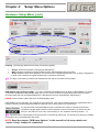
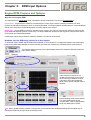
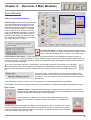
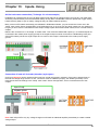
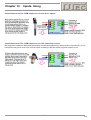
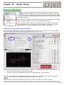
1
DYNertia3 user manual
Manual version 6.4
DISCLAIMER: This software and hardware is provided "as is" without warranty of any kind, either express or implied, including, without limitation, any warranty of merchantability and fitness for a
particular purpose. In no event shall the creators of this software be liable for any direct, special, incidental or consequential damages arising out of the use or inability to use the software. The creators
and distributors of this software shall not be liable for any loss, damages or costs, arising out of, but not limited to, lost profits or revenue, loss of use of the software, loss of data or equipment, the costs
of recovering software, data or equipment or claims by third parties, damage to equipment, or other similar costs.
For continuous product improvement and due to ongoing development, we reserve the right to alter specifications without notice.
WARNING: This hardware and software is protected by law and international treaties. Unauthorized reproduction or distribution of DYNertia3, or any portion of it, may result in severe civil and criminal
penalties and will be prosecuted to the maximum extent possible under law.
DYNertia3 software is copyright- Ross Mclean 2015
DYNertia3 hardware & firmware is copyright- Darren Todd 2015
www.dtec.net.au
1
DYNertia3 user manual
1
STOP !!!
Please read the appropriate ‘Quick Start’ guide for your dyno
type (Chassis or Engine & Inertia or Brake) first.
Actual testing is outlined there!!!.
The following ‘full’ manual contains much detail; by reading the
‘Quick Start’ guide first you will gain a basic understanding of the
concepts and key points required.
There are sample files installed along with DYNertia3 software so you can connect
the hardware and learn to use many of the features without needing to perform actual
tests. It is much easier to study without the noise of a screaming engine!
All examples in this manual use ‘Metric’ units such as kph/Kw/Nm etc. DYNertia3 can
be set in the software to ‘Imperial’ if you prefer mph/Hp/Ft Lb etc!
www.dtec.net.au
2
DYNertia3 user manual
Table of Contents
Chapter 1: Introduction .................................................................................................................................. 8
Introduction ............................................................................................................................................................9
Features ................................................................................................................................................................10
Overview- .........................................................................................................................................................10
Analysing Test Results...................................................................................................................................10
Data Acquisition ..............................................................................................................................................11
File Management .............................................................................................................................................12
Printing .............................................................................................................................................................12
Additional Functions.......................................................................................................................................12
Chapter 2: Hardware Installation................................................................................................................. 14
Hardware Mounting..............................................................................................................................................15
Mounting the DYNertia3 Sensor and Magnet ...............................................................................................15
Alternate Sensors to the supplied one .........................................................................................................16
Mounting the Electronic Control Unit ...........................................................................................................17
Hardware Wiring...................................................................................................................................................18
Power supply connection...............................................................................................................................18
Example of typical wiring (additional devices shown)................................................................................19
‘Linking’ Hardware to PC.....................................................................................................................................20
Chapter 3: ‘Brake’ Style Dyno Setup .......................................................................................................... 21
Brake (Absorber) Style Dyno Setup ...................................................................................................................22
Basic concept ..................................................................................................................................................22
Variations .........................................................................................................................................................23
Calibrating........................................................................................................................................................23
Chapter 4: ‘Setup’ Menu Options ................................................................................................................ 24
Hardware- Setup Menu ........................................................................................................................................25
Brake Inertia Correction (Only in ‘BRAKE’ mode) .................................................................................25
Inertia Mass Constants:............................................................................................................................25
Roller Circumference:...............................................................................................................................26
Tire Circumference....................................................................................................................................26
Sensor/Mass Ratio ....................................................................................................................................26
Mass RPM Limit.........................................................................................................................................26
Reference Voltage Correction..................................................................................................................27
Filtering ......................................................................................................................................................28
RPM Adapter input for Engine RPM ........................................................................................................28
Circumference Calculator.........................................................................................................................29
Software- Setup Menu .........................................................................................................................................30
Run Duration..............................................................................................................................................30
Multiple Monitor Support:.........................................................................................................................30
Data Window Transparency .....................................................................................................................30
Media (Audio).............................................................................................................................................30
Preferred Lambda/AFR Channel..............................................................................................................30
Custom Fuel – Stoic/AFR and Name .......................................................................................................30
Auto Display of Last Run..........................................................................................................................31
Auto Shift Traces Right ............................................................................................................................31
Graph Torque Traces ................................................................................................................................31
Power / Torque Scales ..............................................................................................................................31
Use Actual run Min RPM...........................................................................................................................31
Curve Fitting: .............................................................................................................................................31
Point by Point (Brake Mode) ....................................................................................................................32
Data Consistency ......................................................................................................................................33
Metric / Imperial .........................................................................................................................................33
Run Summary ............................................................................................................................................33
Current Ratio Option.................................................................................................................................33
Hide Windows Desktop.............................................................................................................................33
www.dtec.net.au
3
DYNertia3 user manual
Auxiliary Outputs ......................................................................................................................................33
Edit Existing Run File Name.....................................................................................................................34
Auto Increment copies Run Comments..................................................................................................34
Set Ratio- Change Increment ...................................................................................................................34
DYNertia3 Load Controller .......................................................................................................................35
Password....................................................................................................................................................35
Print Graph Button ....................................................................................................................................35
Communications- Setup Menu ...........................................................................................................................38
DYNertia3 .........................................................................................................................................................38
DYNertia Sensor Test................................................................................................................................38
Weather Watch ................................................................................................................................................38
Interface Port No. ......................................................................................................................................38
Link Button.................................................................................................................................................38
Update Interval ..........................................................................................................................................38
Load Controller................................................................................................................................................39
Printer....................................................................................................................................................................40
Run Time Gauges/Charts (Visible only from ‘Dyno’ Window).........................................................................40
Main Graph Trace Colour (Visible only from ‘Graph’ screen) .........................................................................40
Chapter 5: RPM Input Options..................................................................................................................... 41
Engine RPM, Purpose and Options....................................................................................................................42
Why we need engine RPM ..............................................................................................................................42
Windows used for RPM setup........................................................................................................................42
RPM input Options (6 Available!) ..................................................................................................................43
Summary of your RPM options......................................................................................................................46
General RPM input information .....................................................................................................................46
Chapter 6: Overview- 2 Main Windows....................................................................................................... 47
Two Main DYNertia3 Windows............................................................................................................................48
Dyno Window........................................................................................................................................................49
Record Settings...............................................................................................................................................49
Minimum Run RPM....................................................................................................................................49
Maximum Run RPM...................................................................................................................................49
Current Ratio .............................................................................................................................................49
Mode ...........................................................................................................................................................50
Status..........................................................................................................................................................50
DYNertia3 Hardware Lamp (DYN) ............................................................................................................50
Select or Create DYNertia3 file ......................................................................................................................51
New File Field ............................................................................................................................................51
Increment File Name .................................................................................................................................51
Folder selection (File Paths) ....................................................................................................................51
Run Control......................................................................................................................................................51
Start Run Button........................................................................................................................................51
Correction Factors- .........................................................................................................................................52
User Comments Field- ....................................................................................................................................52
Output controls and Status-...........................................................................................................................52
Speed to RPM (ratio setting)- .........................................................................................................................52
Dial Gauge Displays........................................................................................................................................53
Power & Torque dials................................................................................................................................53
RPM/Speed dial .........................................................................................................................................53
Gauges Mode...................................................................................................................................................53
Data Gauges ON Button ...........................................................................................................................53
Strip Charts ................................................................................................................................................53
Data Dial Gauges.......................................................................................................................................53
Tool Bar Button Functions .............................................................................................................................54
Exit ..............................................................................................................................................................54
Print ............................................................................................................................................................54
RPM/Speed Mode ......................................................................................................................................54
GRAPH/DYNO ............................................................................................................................................54
Selecting Trace to Analyse.............................................................................................................................54
Selecting Trace to Display..............................................................................................................................54
www.dtec.net.au
4
DYNertia3 user manual
Graph controls.................................................................................................................................................55
Data displays ...................................................................................................................................................56
Chapter 7: Weather Corrections.................................................................................................................. 57
Correction Factors ..........................................................................................................................................58
Viewing Weather Data.....................................................................................................................................59
Chapter 8: Loading/Viewing Files ............................................................................................................... 60
Loading of files into ‘Graph’ Window.................................................................................................................61
Previewing (DYNertia3 File Explorer) and Selecting Files ..........................................................................61
Creating / Deleting folders for tests ..............................................................................................................64
Reviewing Audio Files ....................................................................................................................................65
Secondary Graph Window ..................................................................................................................................66
Viewing Files (‘Graph’ Window)..........................................................................................................................67
Adjusting Graph appearance .........................................................................................................................67
Zooming ...........................................................................................................................................................67
Clear Graph Trims ...........................................................................................................................................67
Clear Graph......................................................................................................................................................67
Trace Visibility .................................................................................................................................................67
Chapter 9: Trim, Merge & Join Runs........................................................................................................... 68
Trim a Run.............................................................................................................................................................69
Merge Runs...........................................................................................................................................................70
Join Runs ..............................................................................................................................................................71
Chapter 10: Test Notes- Add/Save .............................................................................................................. 72
Adding Test Notes................................................................................................................................................73
‘User’ notes field .............................................................................................................................................73
Templates..............................................................................................................................................................74
Saving notes and applying to other tests.....................................................................................................74
Chapter 11: Printing & Exporting ................................................................................................................ 75
Printing..................................................................................................................................................................76
General Printing ..............................................................................................................................................76
Offset Correction.......................................................................................................................................76
Select Printer .............................................................................................................................................76
Printing main Graph screens .........................................................................................................................77
Information for Printed Output.................................................................................................................77
Print ............................................................................................................................................................77
Select Page ................................................................................................................................................77
Customising your printout .............................................................................................................................78
Notes to print ........................................................................................................................................................79
General comments for printing......................................................................................................................79
Produce comments on the main graph for printing ....................................................................................79
Exporting data ......................................................................................................................................................80
Chapter 12: Analysing Data (‘View’ Menu) ................................................................................................. 81
Trace Info ..............................................................................................................................................................82
Secondary Graph .................................................................................................................................................82
Individual Trace Set .............................................................................................................................................83
Compare................................................................................................................................................................84
Torque Analysis ...................................................................................................................................................85
Losses ...................................................................................................................................................................86
Lambda / AFR Deviation......................................................................................................................................87
Distance / Speed / Time / RPM Analysis ............................................................................................................88
Slip / Tyre Growth ................................................................................................................................................89
Run Duration Info .................................................................................................................................................90
Point to Point Times ............................................................................................................................................91
XY Graph ...............................................................................................................................................................92
Additional Screens...............................................................................................................................................93
www.dtec.net.au
5
DYNertia3 user manual
Chapter 13: Inputs- Using ............................................................................................................................ 94
Pin Allocations .....................................................................................................................................................95
General Input Notes .............................................................................................................................................96
Important general information .......................................................................................................................96
Wiring inputs for best results ........................................................................................................................96
Connecting Sensors ............................................................................................................................................97
General sensor connection ...........................................................................................................................97
Resistive sensor connection..........................................................................................................................98
Connection of DTec’s ‘Thermo-Amp’ thermocouple amplifier (for K-type sensors) ...............................98
Air/fuel ratio meter connection ......................................................................................................................99
Connection of load cell for Brake (absorber) style dyno’s .........................................................................99
RPM Adapter Input .............................................................................................................................................100
General notes on wiring the RPM adapter input........................................................................................100
Using a DTec ‘RPM adapter’ for the RPM adapter input ...........................................................................100
Basic connections for a DTec ‘RPM adapter’ ............................................................................................101
Connections to suit spark plug wire sensing.............................................................................................101
Connections to suit coil ‘switching’ signals ..............................................................................................101
Connections to suit coil ‘drive’ signals ......................................................................................................102
Connections to suit ‘VR’ (inductive) sensors.............................................................................................102
Sensor Configuration ........................................................................................................................................103
Configuring an input channel using pre-settings......................................................................................103
Creating linear (2 points, straight line) sensor calibrations .....................................................................104
Creating non-linear sensor calibrations .....................................................................................................105
Testing sensor configurations..........................................................................................................................107
Getting the best data.....................................................................................................................................107
‘Data Channels’ Viewing Window.....................................................................................................................108
Sensor Alarm Points ..........................................................................................................................................109
Sensor On / Off (Recording)..............................................................................................................................109
Current Lambda / AFR .......................................................................................................................................110
Data Consistency ...............................................................................................................................................111
Chapter 14: Outputs- Using ....................................................................................................................... 112
Auxiliary Connections .......................................................................................................................................113
Connecting outputs if required....................................................................................................................113
Functions .......................................................................................................................................................113
Chapter 15: Losses Correction ................................................................................................................. 114
’Losses’ System .................................................................................................................................................115
What are the effects of Mechanical Losses?..............................................................................................115
What does Measured Mechanical Loss Correction do? ...........................................................................115
Are these “Losses” worth worrying about?...............................................................................................115
Configuration Window ..................................................................................................................................116
USER Estimated Mechanical Loss Correction ...........................................................................................118
DYNO Mechanical Loss Correction.............................................................................................................119
Chapter 16: Maths Channels ..................................................................................................................... 122
Concept ..........................................................................................................................................................123
Sample expressions, simple ........................................................................................................................125
Testing an expression ..................................................................................................................................125
Variables in detail..........................................................................................................................................125
Creating and saving a math’s expression ..................................................................................................126
Applying an expression to a dyno file ........................................................................................................126
‘Exception’ notifications...............................................................................................................................127
Chapter 17: ‘Help’ Menu............................................................................................................................. 128
Lambda Å Æ AFR Converter .......................................................................................................................129
RPM / Torque / Power Calculator.................................................................................................................129
Open Manual ..................................................................................................................................................129
Configuration reset .......................................................................................................................................130
D3 Snapshot troubleshooting tool ..............................................................................................................130
www.dtec.net.au
6
DYNertia3 user manual
About ..............................................................................................................................................................131
Chapter 18: Trouble Shooting & FAQ’s .................................................................................................... 132
Trouble Shooting- Common Issues .................................................................................................................133
Frequently Asked Questions (FAQ’s) ..............................................................................................................135
Chapter 19: Specifications......................................................................................................................... 136
Specifications .....................................................................................................................................................137
Notes ...................................................................................................................................................................138
Chapter 20: Additions & Changes............................................................................................................. 139
Software V3.xx Changes ...................................................................................................................................140
www.dtec.net.au
7
Chapter 1:
Introduction
Chapter 1: Introduction
Overview and features!
www.dtec.net.au
8
Chapter 1:
Introduction
Introduction
The DYNertia3 Dynamometer package allows for simple and inexpensive "Do It Yourself" construction / upgrade of an
Inertia or Brake Dyno.
Perfect for any one interested in engine / vehicle tuning, testing and modification whether it be car, bike or even model
sized engines.
For those requiring Closed Loop Brake control, please refer to our optional ‘Load Controller’ and additional
documentation
An Inertia type Dyno operates on the principle of calculating the Power required to accelerate a known mass, which is
simply an additional 'flywheel' coupled to the engine or vehicle. The controller senses the velocity of the rotating mass
and outputs this and other data to the DYNertia3 software. No expensive Load Cell is required and repeatability is
excellent.
Brake type Dyno’s use an absorber system (Hydraulic, Friction, Eddy Current etc) to load the engine and the resultant
Torque is measured by a ‘Load Cell’. In ‘Brake’ mode DYNertia3 uses this Torque input and RPM to calculate Power.
The DYNertia3 software package handles all of the functions required for Dyno control: configuration, saving Runs,
correcting for atmospheric conditions, filtering, displaying data, printing, overlaying and analyzing multiple Runs.
A rotation sensor is included with the DYNertia3 Controller; you simply attach a magnet (supplied) to the Inertial Mass /
Brake or drive system. Optionally, we can supply a Hall sensor designed to sense a metal ‘target’ rather than a
magnet, allowing a metal protrusion or tooth to be used as the Sensor "target".
For Engine or Chassis Inertia Dyno's we also provide a comprehensive guide to assist in the design and construction of
the Inertia Assembly. All you need in addition to this is the DYNerta3 package and a PC with a USB port.
Five analogue data channels and one digital input (secondary RPM input) are available for displayed and recording these are completely flexible and can be used for sensors such as Air Fuel ratio, Exhaust Temperature, Pressure, Load
Cell, secondary RPM etc. Two ‘Math’s’ channels can be created from any of the existing data (create your own
formulas), just think of the tuning possibilities!
www.dtec.net.au
9
Chapter 1:
Introduction
Features
OverviewSuitable for chassis and engine dyno designs, either direct or indirect drive to the inertia flywheel. Power measurement
can also be taken from a ‘load cell’ for use on brake style dynos (e.g. water, eddy current, hydraulic, friction). DYNertia3
does not control the actual load on a brake style dyno, the load must be controlled manually (i.e. it’s not closed loop).
For closed loop control of a load please see our optional ‘Load controller’ unit and additional documentation.
Software provided handles all data management, analyzing and graphing required for your dyno project with powerful
features yet a ‘clean’ interface. Both Metric and Imperial modes are provided, Power, Torque and setup parameters are
changed from kph/Kw/Nm/ºC to mph/Hp/Ft Lb/ ºF etc.
Comprehensive Manual provided, also design & construction information is available for the mechanical dyno system,
including an Excel spread sheet to assist with choosing and calculating the moment of inertia for your requirements.
Included magnetic sensor (hall effect) has an indicator for diagnostics. Integrated ‘optical isolation’ circuitry in the data
acquisition systems helps limit ignition interference and provides PC protection.
As an inertia dyno, accuracy is only limited by mechanical system variation, internally each rotation is timed to 1µs (1
millionth of a second). Dual microprocessors share the data acquisition and precision timing tasks.
Ideal for portable applications (track days & exhibitions). Power supply can be from a simple 12VDC battery, 7 to18VDC
is required, e.g. a cordless drill or bike battery is ideal! We recommend a battery as resistance to interference and data
acquisition signals is far better than with a ‘plug pack’!
Compact, approximately 110L x 83W x 45H (mm) with a small remote sensor for easy adaptation to your design.
No ignition system adapters are needed for RPM sensing. It can determine engine RPM from shaft RPM by ‘learning’
their relationship (ratio). Up to 8 gears can be learnt and later selected for quick testing in any gear; the ratio can also be
manually entered if no tachometer, simply based on number of sprocket teeth (e.g. for chain drive kart engine dynos).
If an engine RPM input (not otherwise required) from the engine is available, then this can not only be used as engine
RPM but also means the difference between engine and shaft/flywheel RPM can be plotted to show clutch engagement
RPM or reveal wheel slip on a chassis dyno.
Inertia value for up to 3 Inertia mass flywheels can be stored and easily selected for designs with adjustable Inertia mass
to tailor to engine characteristics.
Compensation for Dyno Inertia during ‘brake’ testing is easily applied. Great if you have an inertia dyno, but wish to add
an additional load (brake/retarder) for ‘running in’ engines or ‘steady state’ testing.
Updates to the basic DYNertia3 software will be available FREE as we continually seek to improve our product.
Analysing Test ResultsSupports multiple monitors, if a second monitor is available then key Windows can be viewed separately to allow clear
analysis, even if viewing and comparing many test results.
Overlay up to 10 Power and Torque graphs simultaneously, including the ‘Last Run’ which automatically appears after
your Run is completed. Run trace color sets are user selectable, however ‘Last Run’ always graphed in red for quick
identification.
Analyse and compare test results by easily ‘hiding’ any particular Run trace or quickly replacing with other saved Runs
for comparison.
A reference Run trace can be locked so that it always stays on the screen for comparisons against other tests.
Up to 4 sets of Runs can be merged to create a brand new 'averaged' Run. Perfect for getting the most from
analysis. The new generated file appears just like any other in DYNertia3. Comments are automatically attached that
reveal the individual runs that it was generated from for future reference.
All 5 analogue channels are recorded with each Run for analysis and their value at the cursor are shown in a floating
'data box' (which can also be saved to ‘clipboard’). DYNertia3 can overlay 2 chosen data channels with the existing
Power and Torque traces for display or all of the data for any trace can be shown in a separate single Window for
detailed analysis.
Select a graph trace; an onscreen cursor makes the dials (power, torque and RPM/speed) display exactly what was
happening at that point in the test Run.
Advanced torque analysis is provided to graphically display ‘area under the curve’ and related statistics for comparing
multiple traces.
www.dtec.net.au
10
Chapter 1:
Introduction
Analysing Test Results (cont.)The percentage difference between a reference trace and the remaining traces can be shown graphically, for all data.
Instantly see where each modification either improves or degrades performance compared to other runs. Great tool!
Lambda / AFR deviation is shown in a special Window that allows you to set a target value, it shows you where and by
how much the real test results varied (essential for quick mixture tuning). Obviously an AFR meter must be connected!
Select any RPM/speed points and the time between them is shown for all Runs (up to 10), clearly reveals ‘real world’
acceleration improvements after modifications. Best performing Runs between all points are highlighted.
Full data table display of ‘point by point’ Power, Torque, RPM and Speed are produced for detailed study and can be
exported directly into Microsoft Excel (with field headings included) or a text file (comma delimited ASCII, CSV.) can be
generated, even the main graph view can be exported as a bitmap image (‘.bmp’) for further analysis and file sharing.
The relationship between distance traveled, time elapsed, Speed and RPM can be studied in a graphical analysis
screen.
XY graph, choose any data to plot against another and display values at the cursor.
Math’s ‘Expressions’ (formula) can be applied to any existing data to generate an additional 2 data channels. A powerful
tool is provided to easily write, test and apply your concepts.
Click on the Run of interest to show all the data that relates to it. The test conditions, max readings, set up details or any
of your personal notes that are saved along with each run can all be reviewed.
Full manual ‘zoom’ available on Power, Torque and RPM displays to display selected graph regions of interest.
Runs can be ‘trimmed’, the lower and upper speed section of graphs can removed if visually required (e.g. if tests start
and finish RPM were inappropriately set) and the Run re-saved.
User selectable ‘Trace Shift’, the last 10 trace sets are always displayed (each new test trace ‘shifts’ the oldest one out
of selection) - great when performing comparisons.
‘Auto Load’ your graph after a Run – can be selected to automatically switch to the graph display after each test Run or
you can opt to do as many Runs as you like in quick succession and analyse as a graph later. A brief test summary is
also immediately available after each test Run is completed.
Onscreen graph legend to rapidly identify Run trace set colors and filenames and a run summary is available to give the
key data for all the selected runs in one concise table.
Data corrected for weather conditions with world standards (SAEJ607, SAEJ1349, DIN70020 or uncorrected). The
environmental conditions and resultant correction factor are stored with each Run. Data can be manually entered or
‘Weather Watch’, automatic updating weather station is available as an option (USB to PC).
Data AcquisitionData acquisition of 5 analogue input voltages is incorporated (‘common’ ground). This allows the monitoring of variables
such as air fuel ratio, exhaust temperature etc.
Inputs can be 0-5V or 0-15V (each channel has a range selection switch)
Resistive sensors, such as standard automotive temperature sensors, can be easily connected as each channel has a
selection switch that enables an internal ‘pull up’ resistor (just connect the sensors 2 wires directly to DYNertia3!).
A data logging function is provided allowing the 5 input channels (plus the digital RPM input) to be logged to the PC. The
logging rate can be set and the data is saved (with field headings included) as a text file (.CSV) for later analysis in
Microsoft Excel etc.
Input data can be viewed separately (can even be displayed on separate screen if dual monitors used) or is available
whilst performing testing. Minimum and maximum alarms can be set to alert if sensors detect anything outside an
acceptable level (lean mixtures, engine temperature overheat or oil pressure loss as examples).
The input channels are fully scalable, even for non-linear sensors. Many sensor choices are already pre-calibrated and
DYNertia3 software doesn't just display the input voltage measured, a table for each input allows it to be calibrated and
displayed in any units you choose (eg Lambda, air/fuel ratio, degrees, PSI etc).
For configuring non-linear sensors, such as automotive style temperature sensors, there is a tool provided that just
requires 3 test points to be entered and it creates a full calibration table.
www.dtec.net.au
11
Chapter 1:
Introduction
Data Acquisition (cont.)Simple screw type terminals on a removable terminal plug allow for quick and easy sensor wiring. Both a 5 Volt and 12
Volt output to power auxiliary sensors is also present if required.
An additional digital channel is provided if you wish to have engine RPM directly measured (via a Hall sensor or DTec’s
‘RPM adapter’). This option can help reveal tyre slip/growth on a chassis dyno or centrifugal clutch engagement RPM.
There is a dedicated analysis screen to examine slip/tyre growth.
File ManagementDesigned to perform testing quickly- common user settings are saved to reduce set up times and any personal notes
you’ve entered in the provided form (general, vehicle, owner details etc) can be saved as a ‘template’ and applied to
other runs to save re-entering the details, even copies the Run’s set up details. Files can also be set to ‘auto name’, the
file name simply increments with each test (and can carry over any personal notes), no need to even re-enter a name.
Advanced previewing function (‘DYNertia3 File Explorer’) shows graphs, summary details and the data table of all saved
runs, this allows quick selection for loading into the main graph screen or for file management purposes. A cursor is
even available to highlight points of interest on the graph and indicate that same location in the data table- no more
browsing through cryptic file names!
User configurable directories- have as many separate directories to store your runs in as required and file protection can
be applied to prevent individual files from being accidentally changed or overwritten if required.
PrintingColor print outs of your chosen graph or overlaid graphs (up to 5 printed on same graph) is only a mouse click away,
complete with preview. A report page is also generated that has a summary of all the important test conditions, max
readings, date, time, company logo, graph notes etc.
Printouts includes Run trace sets legends, colors and filenames, the graphs ‘grid lines’ can even be turned off!
Comments can be placed on the graphs to appear on the printouts.
Printing of specific areas of interest can be performed using the manual ‘zoom’ function.
Additional Functions‘Ponit by Point’ testing mode for brake style dyno’s allows recording of individual data points at the press of a button.
These individual data sets are then combined to construct a conventional Run trace for easy analysis and comparisons.
For dyno competition entertainment, after a run maximum Power and Torque can be displayed in large format for crowds
to easily see (result in both imperial and metric units).
Graphs are fully auto-scaled, Power, Torque and RPM scales are automatically configured for optimal display.
Flexible options for performing a test; a Run can be from ‘start’ command to ‘stop’ command or from ‘start’ command to
zero power. A minimum speed can also be specified and data below this will be discarded, this eliminates any different
start points of tests due to operator error.
All dial gauges have digital displays incorporated.
Gauges display ‘real time’ data during monitoring or setup. Ideal for steady state tuning with a brake type dyno! (only
RPM is displayed 'real time' in Inertia mode)
Data ‘Smoothing’ that is applied to the Power traces is adjustable to ensure you don’t miss out any detail but still end up
with optimal appearing graphs.
There is a “Losses” function that can be used to measure and apply a correction to data for mechanical losses in your
dyno system like friction and windage (typically very small) even or/and for driveline losses due to friction.
DYNertia3 is fully isolated (optically) from the PC, this helps prevent any damage to the PC from incorrect connections
(power DYNertia3 from a battery source for this full isolation!). DYNertia3 is also protected from reversed polarity supply
connection.
A ‘system in motion’ (“Run”) output is available that is active as long as the flywheel is rotating, or a function is used that
may result in rotation. This can directly control a relay to operate safety control systems/warnings if required or for
automatic fan controls etc.
www.dtec.net.au
12
Chapter 1:
Introduction
Additional Functions (cont.)An ‘Auto Brake’ output is available that can directly operate a relay for an automatic brake (e.g. eddy current) for slowing
the flywheel down if you wish, or an automatic cooling fan for cooling friction style brakes. The time it’s active for after a
test Run is adjustable in the software. The output can alternatively be operated manually in the software and will be
active for either a short time or continuously.
A ‘user controlled’ output is available can directly operate a relay, it is manually turned on or off from the software and
can be used for any general purpose function e.g. remotely turning on a cooling fan, pumps wheel clamps etc.
Tools to work out the moment of inertia of your dyno system, calibrate non linear sensors, convert air:fuel ratios to
Lambda and for analysing relationships between Power / Torque / RPM are incorporated.
Keyboard ‘shortcuts’ assist with easy operation and an inexpensive and commercially available remote ‘page turner’ (the
device often seen used for PowerPoint presentations) can be used as a remote control that can start/stop Runs, turn the
gauges on/off and allow automatic file incrementing (no need to type in a new name). Very convenient if operating both
the vehicle and the dyno single handedly.
www.dtec.net.au
13
Chapter 2:
Hardware Installation
Chapter 2: Hardware Installation
Hardware mounting
Alternate sensor options
Basic power wiring (see ‘Inputs- Using’ chapter for full details)
‘Linking’ hardware to the software
www.dtec.net.au
14
Chapter 2:
Hardware Installation
Hardware Mounting
Mounting the DYNertia3 Sensor and Magnet
DYNertia3 times the rotational period of a component by sensing its position magnetically. The included sensors ‘face’
contains a magnet sensing ‘Hall Effect’ switch. The sensor detects the position of the magnet attached to the rotating
dyno flywheel/load brake/shaft and processes to trigger the timing procedure.
NOTE: The rotation sensor system is the main RPM input used by DYNertia3 for Power calculation and therefore must
always be setup for operation. If you choose to also use the engine ignition system (or other source) as a secondary
RPM input then please read the chapter on ‘RPM Input Options’ in this manual regarding this optional input!
A small (9mm x 1.5mm with 3mm mounting hole) but very powerful ‘rare earth’ magnet is included with the kit. The
magnet is small as this reduces the forces involved when rotating so it is easier to secure safely.
Do not mount the magnet at the perimeter of the dyno flywheel/shaft/sprocket etc. as the centrifugal forces will be
highest; choose a location towards the centre area. The magnet is also very fragile and must be handled with care!
There are several options to mount the magnet and we suggest a combination to ensure safety and reliability.
NOTE: The included sensor will only detect the ‘South’ Pole of a magnet, so the magnet must be have the South Pole
(marked with red paint) facing the sensor!!
Preferred method (securest)Drill a shallow 9mm diameter location hole so the magnet just
protrudes. Also drill and tap for 3mm screw (2.5mm drill size is usual
for 3mm tapping). Short (min 6mm) screw inserted into magnet. Do not
over tighten or magnet may crack!
Magnet glued and screwed to dyno flywheel with South Pole outwards.
Mounting by screwing/gluing flat to dyno flywheelDyno flywheel is drilled and tapped for 3mm screw (2.5mm drill size is
usual for 3mm tapping). Short (min 6mm) screw inserted into magnet.
Do not over tighten or magnet may crack!
Magnet glued and screwed to dyno flywheel with South Pole outwards.
Mounting by gluing- Epoxy glue can be used to secure the magnet to the rotating dyno flywheel; we do not
recommend just this approach. If it becomes loose it can fly off dangerously! At least if doing this then drill a recessed
hole as above.
The sensor face must be positioned 1.5 - 2mm from the
magnets South Pole (or the head of the screw if one is used
to secure magnet).
www.dtec.net.au
15
Chapter 2:
Hardware Installation
Hardware Mounting (cont.)
A16mm diameter hole is required to mount the sensor. Do not over tighten the lock nuts or they will be damaged. A
small ‘blob’ of silicon sealant or similar is applied to the edge of the nuts to stop them loosening with vibration.
*Tip- With power connected to DYNertia3
the status LED (next to the sensor
connector) can be used to confirm sensor
operation. When the magnet is under the
sensor then the LED should be OFF.
KEY POINTS- 1.5 – 2mm gap. Safe magnet mounting, South Pole (marked with red
paint) of magnet facing towards the sensor!
Alternate Sensors to the supplied one
DYNertia3 can accept other types of sensors if you prefer. The sensor input terminal is a digital input; it will not accept
voltage from an inductive sensor (VR). The ‘signal’ terminal of DYNertia3 needs to be ‘pulled’ to ground when a target
object is detected. Sensors that switch to ground like this are called ‘open collector’ style and include most industrial
proximity sensors and also the majority of automotive camshaft sensors (‘Hall’ type).
NOTE: If you are unsure please just contact us for help; we are not responsible if you damage the unit from incorrect
connection!
Hall sensors- Hall sensors are ‘switching’ style sensors and are compatible, they are available to detect either magnet
or metal ‘target’ objects. This may be a good choice if you wish to detect a rotating metal object rather than a magnet
like the provided sensor does i.e. perhaps you have a protruding ‘key’ in a shafts key way. A common metal sensing
sensor example (shown below) is the ‘Honeywell 1GT101DC’ sensor or most automotive camshaft sensors are good.
Optical sensors- The sensing ‘face’ contains an infrared (invisible) light transmitter and a matched detector. The light
beam is reflected from a suitable object, normally reflective tape attached to the rotating ‘flywheel’. Optical sensors are
very easy to adapt to designs as all that is required is a reflective tape be applied to the rotating component. They do
however need to be set at the correct distance and have a stable mounting. The previous generation of dyno called
DYNertia2 solely used this method.
DTec can provide these alternate sensors if required. Please contact us for options and pricing.
www.dtec.net.au
16
Chapter 2:
Hardware Installation
Hardware Mounting (cont.)
Mounting the Electronic Control Unit
Strong vibration may also destroy the sensor and control unit (as with all electronics) so it is important to consider
mounting arrangements carefully.
NOTE: Engines with CDI ignitions, especially in conjunction with copper core spark plug leads and non-resistive spark
plugs can generate large electrical interference for all electronics including PC’s. It is very important to apply the
following mounting and cable routing suggestions to avoid any problems!
It is very important to keep the PC, DYNertia3 and it’s cabling well away from large sources such as ignition systems-
1. Mount the DYNertia3 sensor unit at the furthest distance from the engine as possible.
2. Route all cables as far as possible away from the engine and keep the PC at a distance. Coil any spare cable up
neatly at the PC.
3. It’s best to route cables behind a protective metal tubing or keep separated from the engine by the metal of the dyno
frame or shields.
4. Use resistive spark plugs and suppressed plug leads (at least during testing).
*Tip- A suppressed spark plug lead from a car can be put in series with the existing spark plug to reduce interference.
5. Follow the wiring advice in the “Inputs- Using” chapter on wiring if measuring from additional sensors.
‘P’ clips are provided in the kit. They must be used to secure the USB
lead, power and sensor leads close to the DYNertia3 control box. The
aim is so that the leads are completely prevented from movement, as
this will place stress on the connectors and wiring.
www.dtec.net.au
17
Chapter 2:
Hardware Installation
Hardware Wiring
Power supply connection
Please see chapter called ‘Inputs- Using’ of this manual for full wiring details on connection of data acquisition devices,
below we just cover the power supply connection required for basic operation.
Power supply can be from a simple 12VDC battery, 7 to 18VDC required. DYNertia3 draws less than 100mA so very
little demand is put on a battery e.g. a cordless drill or bike battery is ideal!.
A power pack connected to mains is NOT recommended, especially if data acquisition is being used. The resistance to
interference and stability of the data acquisition signals is generally much better with a battery! This is very dependant
on the dyno installation, PC used and engine types being tested (as to how much interference they produce).
Full isolation protection (optical) for the PC is only provided when DYNertia3 is powered from a battery source.
NOTE: Very low battery voltage (less than 7VDC) will cause poor sensor operation and erratic results. Please monitor!
With power connected to DYNertia3 the status LED (next to the sensor connector) will blink twice at first to indicate
microprocessor is initialising. After this the LED will illuminate to indicate power, but it will turn off whenever the magnet
is under the sensor. The LED is also off when DYNertia3 is in any mode that requires communication with the PC. Don’t
assume there is a power supply problem based solely on LED operation!
www.dtec.net.au
18
Chapter 2:
Hardware Installation
Hardware Wiring (cont.)
Example of typical wiring (additional devices shown)
Please see chapter called ‘Inputs- Using’ of this manual for full wiring details on connection of data acquisition devices.
For brake type dyno’s there will be a load cell and amplifier to be connected to channel 5, this is covered in more detail
in the Brake dyno ‘quick start guide’.
www.dtec.net.au
19
Chapter 2:
Hardware Installation
‘Linking’ Hardware to PC
1. Follow the software instructions exactly (separate sheet) and install DYNeria3 software.
2. Do not have other programs running when using DYNertia3, background processes can interfere.
3. When you first run DYNertia3 you will be shown this Window. Press the “continue offline” button, this is necessary
as DYNertia3 does not yet know what PC port your hardware is connected to, it must be first ‘Linked’ to know this.
Once ‘Linked’ DYNertia3 will automatically find the hardware in future when it is connected, powered and the software is
started. If you plug DYNertia3 hardware into another USB port you may need to re-link.
This screen will also appear whenever DYNertia3 is started and the hardware is not connected, powered or ‘Linked’.
Pressing the “Continue Offline” button allows you to continue to use DYNertia3 to view and analyse data ‘off-line’ (i.e.
with no hardware connected).
4. Power your DYNertia3 hardware (red LED must blink at first) and plug the USB in, wait now for the PC to recognise
USB is connected, select the menu option “Setup” and then choose “Communication” and press the “LINK” button to
automatically configure the port interface.
www.dtec.net.au
20
Chapter 3:
Brake Style Dyno Setup
Chapter 3: ‘Brake’ Style Dyno Setup
Setting up a brake (absorber) style dyno, instead or in addition to an
Inertia style Dyno!
The following information regarding brake type dyno’s
assumes an ‘open loop’ dyno system.
If you have our load control system for ‘closed loop’ control
(or servo throttle control) then you will also need to read its
separate manual. The contents of this manual are still relevant,
there are just some extra details on setting up hardware and
on operating the extra software features.
www.dtec.net.au
21
Chapter 3:
Brake Style Dyno Setup
Brake (Absorber) Style Dyno Setup
Basic concept
Brake (‘retarder’ or ‘absorber’) style dyno’s rely on a device to apply load to the engine, this can be electric (eddy current
or generator), water, hydraulic or friction, we will use the term ‘brake’ for any of these load devices. The device
absorbing the Power is generally mounted so its case can rotate as a load is applied. It is this rotation force that is
measured to calculate the Torque.
The case is attached to a ‘load cell’ (the sensor measuring the force) via a ‘Torque arm’ that transfers the rotary motion
into a linear one applied to the sensor.
Most designs use an electronic load cell to measure the torque but some dyno’s use a pressure sensor fitted into a
hydraulic cylinder as a load cell. Older designs even just had springs opposing the ‘Torque arm’ movement and use a
position sensor to measure the spring’s deflection (linear potentiometer).
The length of the Torque arm acts as a lever, so this length can be selected based on the working range of your load cell
for appropriate sensitivity.
The DYNertia3 controller senses the velocity of the rotating brake/retarder or its shaft, handles the precision timing
required (1 millionth of a second) and outputs this data, along with the load cell information to the PC for analysis and
storage.
The included 'DYNertia3' software package handles all the functions required of dyno acquisition: setting up, saving
runs, correcting for atmospheric conditions, filtering, displaying data, printing, overlaying and analyzing multiple runs.
Notes: Basic DYNertia3 system does not control the actual brake/retarder load, this must be manually controlled. It has
no ‘closed loop’ function i.e. you cannot enter an RPM and have DYNertia3 vary the load to maintain that RPM
automatically. This would raise the price of DYNertia3 unacceptably if we included this ability in the base unit.
For closed loop control of your load please see web site for our optional ‘Load controller’ unit and additional
documentation.
It can be very difficult to allow steady rising of the RPM for a ‘run’ without a good control system for your load, friction
brake systems are particularly difficult to operate smoothly and are often best operated for brief ‘steady state’ tunning
(‘Point by Point‘ mode is ideal). Excessive Inertia in your system can also cause difficulties on low power engines i.e. the
inertia load can end up limiting the acceleration during a test and not the load absorber device.
www.dtec.net.au
22
Chapter 3:
Brake Style Dyno Setup
Brake (Absorber) Style Dyno Setup (cont.)
In Brake mode, DYNertia3 uses Torque data from the load cell and engine RPM (calculated from the dyno’s included
sensor or from RPM Adapter input) to correct Torque and calculate Power. If the ratio’s are set incorrect (or RPM
Adapter input is poor if it’s being used for RPM) then the readings will be incorrect i.e. if you just use roller RPM on a
chassis dyno then Torque will be shown as it appears at the roller only and not related to engine RPM. This is called
‘Tractive Torque’ (Torque at the tyre) and will be higher than engine Torque due to the gears multiplying effects. It is
really the Torque delivered to the road and can be used as an effective tunning tool due to the increase in Torque
resolution!
Variations
As noted earlier, some brake style dyno use a hydraulic cylinder (like a vehicle ‘master cylinder’) as the ‘load cell’, by
fitting a pressure sensor into the cylinder this provides the torque output. Alternatively some very old systems use a
spring assembly to counter the brakes rotation and then measure the displacement of this with a linear potentiometer
(position sensor).
Both can be interfaced into DYNertia3!
Mechanical instability will cause poor quality data, some old friction style brake dyno’s even have shock absorbers to
dampen movement (those just mentioned with springs in their load measurement system).
Calibrating
Most load cells only produce a tiny voltage change as the load increases; they therefore generally require an amplifier
(often called a ‘transmitter’ or ‘strain gauge amplifier’) to be wired in.
The sensor input in DYNertia3 must be calibrated in metric Newton meters, Nm (see menu ‘data/sensor calibration’) and
the load signal must be connected to input channel 5.
Calibration is performed by noting the voltage from the load cell at rest (this is zero Nm) and then apply a known weight
to the arm so that this represents the torque level you wish to measure (you can add an extension to the arm so less
weight is needed if required during this calibration) . Take the voltage reading from the sensor when the weight is
applied and enter this into the sensor calibration table along with the calculated torque (as below).
Torque = load (weight in Kg applied x 9.80665) x length of torque arm in meter’s
Therefore, if I had 2 meter arm (centre of dyno bearing to arms end) and hang 30kg off the end I am applying a torque of
30 x 9.80665 x 2 = 588.4 Nm
To help you imperial guys out there: 1 pound = 0.4535924 kilogram and 1 foot = 0.3048 meters
So, if I had 10mV at no load and 2000mV (2V) at 588.4 Nm then these are my two calibration points I need.
In the chapter called ‘Inputs- Using’ are the details on actually setting up DYNertia3 software to suit the calibration
information you have calculated (even if you have non-linear sensor data).
Note: There is no need to produce the full Torque load on the load cell for calibrating, though accuracy will suffer if too
light a weight is used. To ensure the full load cell range is covered it’s best to take your two readings and calculate how
many Volts per Nm the load cell produces, you can then tell what will be the Nm output at the full 5V (5000mV) range
that DYNertia3 accepts. This will give you a maximum value that exceeds your calibration weight and means you do not
have to apply excessive strain on your system when calibrating.
(in the above example 1990mV covered a range of 588.4Nm so that load cell system puts out 3.4mV per Nm applied)
Note: DYNertia3 can still perform power calculations from a load cell as well as the inertia mass whilst performing a run
i.e. inertial correction can be applied (see ‘Setup/Hardware’ menu to activate).
www.dtec.net.au
23
Chapter 4:
‘Setup’ Menu Options
Chapter 4: ‘Setup’ Menu Options
Hardware setup
Software setup
Communications setup
Sensor setup
Losses setup
Main Graph Appearance setup
Configuration reset
www.dtec.net.au
24
Chapter 4:
‘Setup’ Menu Options
Hardware- Setup Menu
Brake / Inertia Button: Determines if you are using a brake
(retarder/absorber) type dyno or an Inertia type dyno. If you select a brake
style dyno then DYNertia3 will expect to see a ‘load cell’ input into channel 5
of the data acquisition connector. This will be used as the primary torque
input for Power calculations rather than the inertia value.
Brake Inertia Correction (Only in ‘BRAKE’ mode): If you have a brake style dyno and are
performing fast ‘ramp rate’ runs (or if you have a brake attached to your inertia dyno) then the
inertia of your dyno may be considerable. If you select this option, and have the Inertia value
correctly entered, then DYNertia3 will basically operate as both Inertia and brake dyno
simultaneously i.e. it will calculate the power used to accelerate the mass as well as derive
the power from the load cell.
Helpful Tools!
Inertia Mass Constants: The dynos “Primary Mass” (the main dyno ‘flywheel’) inertial value is entered here (see
“MOI” button for a tool to help calculate if not already known). If the dyno design incorporates multiple selectable dyno
flywheels then their values can be entered in “Second Mass” and “Third Mass” to allow quick selection in main Dyno
screen.
These extra masses are added to the primary inertia value when selected in the ‘Dyno’ screens “Record Settings” box.
www.dtec.net.au
25
Chapter 4:
‘Setup’ Menu Options
Hardware- Setup Menu (cont.)
Roller Circumference: Used for chassis dyno’s to allow speed in kph/mph to be displayed if
required (see “CIRC” button for a tool to help calculate if not already known).
The entry screen for roller circumference is only revealed when this button that
indicates you have a chassis dyno is selected.
Tire Circumference: Optionally is used for engine dyno’s if you wish to display speed in
kph/mph as oppose to just RPM (see “CIRC” button for a tool to help calculate if not already
known). The road speed can be simulated as the dyno will now know what distance would be
travelled for every turn of the drive shaft.
The entry screen for tire circumference is only revealed when this button that
indicates you have an engine dyno is selected.
Note: Units will be metric or imperial based on your choice in menu “Setup/Software” (Imperial or Metric)!
Sensor/Mass Ratio: On some special purpose dyno applications it may be that there is extremely
low rotation speed and therefore limited flywheel/roller timing data. This feature allows designs such
as this to drive a sensor wheel via gearing (or friction contact) at a higher RPM and this can have
the sensor trigger target speed applied rather than the flywheel e.g. if the sensor was spinning twice
as fast as flywheel/roller then a value of 2 would be required.
It is also used where the sensor is not actually mounted on the flywheel/roller but on another shaft
that rotates at a different speed to the inertial mass.
Note: Trying to use this feature to allow triggering from multiple triggers on the flywheel/roller will result in poor data
quality; it will need excessive filtering to smooth out the ‘jitter’ from tolerances between your trigger targets.
Mass RPM Limit: You can apply an RPM limit alarm to your system if you wish i.e. if there is
a maximum safe limit you wish for your mass/flywheel not to exceed. If DYNertia3 detects an
over speed condition it will give very obvious alerts to the danger and force an end to your
test session.
www.dtec.net.au
26
Chapter 4:
‘Setup’ Menu Options
Hardware- Setup Menu (cont.)
Reference Voltage Correction: A tiny voltage error may be
present in DYNertia3’s internal 5 Volt supply, this option is
available to correct for this variation. This adjustment is rarely
required as the 5 Volt is very precise. Simply measure the
voltage between the ground and 5V output terminals on the
data acquisition connector and enter the measured voltage.
*Tip- This voltage can be also used to correct for sensor errors (if applicable to all channels), but this is really best done
by modifying the sensor configuration table to 'trim' the result, see chapter “Inputs- Using”.
Brake Hardware Output: Is a timed output that can operate an automatic brake for slowing
the flywheel down if you wish, or an automatic cooling fan for friction style brakes. The
output goes active from after a run is stopped and remains on for the time set here. The
output can alternatively be briefly operated for 2 seconds (not adjustable) by manually
selecting (icon on both Graph and Dyno screen), this allows for setting up safely and also
brief braking pulses. If not allocated to a brake; this output would be perfect for remotely
turning on a cooling fan etc
This Indicator (Visible in both DYNO and GRAPH screens) displays the state of the output, alternatively,
‘Left’ clicking on the Icon on these screens will briefly operate the output for 2 seconds (not adjustable),
this allows for setting up safely and also brief braking pulses. A ‘Right’ click will turn on the output
continuously until another ‘Right’ click is done again i.e. ‘Right’ click toggles the output state.
Note: Further details for the output functions are outlined in the chapter “Outputs- Using”
www.dtec.net.au
27
Chapter 4:
‘Setup’ Menu Options
Hardware- Setup Menu (cont.)
Filtering: The ‘Filtering’ determines the level of smoothing applied
•
•
•
‘Gauges’ effects the operation of the gauges (dampening).
‘ADC’ (Analogue to Digital Converter) applies to the 5 data channels that may be used.
‘Graph’ applies to dyno power graphing. This has the effect of displaying data that is not so wildly changing due
to small cyclic variations in engine firing and dyno mechanical tolerances.
*Tip- Too large a ‘Smoothing’ numbers and disturbances that may be of interest can be hidden.
RPM Adapter input for Engine RPM: If you have a suitable input adapter (such as DTec’s ‘RPM Adapter’) or sensor
connected to DYNertia3’s RPM Adapter input then you can choose to have this engine RPM value used for various
functions rather than the calculated RPM (which is derived from the main flywheel/roller speed sensor).
NEVER connect ignition system directly to the RPM Adapter input!
RPM Adapter input is required if ‘slip’ analysis is to be performed. ‘Slip’ is dyno RPM compared to engine RPM, this is
handy for checking clutch engagement RPM or looking for loss of tyre traction on a chassis dyno.
It is important that if the RPM Adapter input is used then the number of pulses received that
represents a single engine rotation must be entered. It can be fractional e.g. 4 strokes only fire
every 0.5 rev (which is once every 2 revolutions!) so “0.5” would be entered (2 stroke = “1”)
*Tip- Could be used to compensate for sensors that are connected via gearing e.g. if a hall sensor is picking up rotating
bolt heads on an intermediate sprocket carrier.
NOTE: Read the chapter “RPM Input Options” in this manual for full setup details and
“Inputs- Using” chapter for connection!
www.dtec.net.au
28
Chapter 4:
‘Setup’ Menu Options
Hardware- Setup Menu (cont.)
Load Controller: These functions are for the ‘closed loop’ load controller unit. The button is not available
unless the optional load control hardware is connected and linked. Please see our web site for this option!
There is an additional guide provided to fully explain the operation of these features and the related screens
that are not shown in this manual.
Circumference Calculator: Tool to help calculate your
rollers circumference if you do not already know it.
Units will be metric or imperial based on your choice in menu
“Setup/Software” (Imperial or Metric). Pressing the “Circ” button will
transfer this circumference value into the ‘Setup/Hardware’ menu field.
Moment Of Inertia Calculator: Tool to help you calculate the Moment of Inertia (MOI) of your dyno. If the
dyno design incorporates multiple selectable flywheels then their values can be saved separately as a “Second
Mass” and “Third Mass”.
Once the values of
components have
been entered into
the rows they can
be saved (or loaded) for later use and
reference, they can even be directly
transferred into the “Inertial Mass
Constants” field in this ‘Hardware’
menu.
Simply press one of the numbered
buttons and the MOI value will be
recorded as that mass.
‘Eraser’ button clears the filled in fields so new values can be entered.
www.dtec.net.au
29
Chapter 4:
‘Setup’ Menu Options
Software- Setup Menu
DYNO Correction Systems: This allows tests to be corrected to a standard set of atmospheric conditions for
consistency as the environmental test conditions change. Correction to world standards SAEJ607, SAEJ1349,
DIN70020 or uncorrected can be applied. SAE J607 is chosen by default as it is in widespread use. See chapter
“Weather Corrections” for details.
Run Duration Calculated until: Run time duration displayed in the data will start at the press of the “start run” button
(or F12) and end at these two options, either ‘stop’ pressed (or F12) or zero Power detected.
Multiple Monitor Support: DYNertia3 can display its data across two monitors, this allows comfortably analysing large
amounts of data. You can select what monitor displays the main Graph Window or other selected Windows.
Data Window Transparency: Sets the transparency level of the ‘floating’ data box that is used in several analysis
screens & also the main Graph Window. ‘Transparent’ menu then controls the function from within the data box!
Media (Audio): Enables an audio input via the PC’s microphone. This can be used to simply save a commentary
during a test or to record the actual engine noise. For further details see chapter “Overview- 2 Main screens” for details
of controls on Dyno Window and also chapter “Loading/Viewing files” regarding “reviewing Audio files”.
Preferred Lambda/AFR Channel: Set to input channel your AFR meter is connected to, saves re-selecting in later
analysis Windows.
Custom Fuel – Stoic/AFR and Name: If you are using a special fuel that is not in our standard list, then you can enter
a custom AF ratio here. This is only required if you are using this fuel for analysis using AFR, it is not required for
working in Lambda. See chapter “Inputs- Using” for details of ‘Current Lambda/AFR’ analysis Window.
www.dtec.net.au
30
Chapter 4:
‘Setup’ Menu Options
Software- Setup Menu (cont.)
Auto Display of Last Run: When selected, DYNertia3 will automatically open the Graph Window and add the test Run
just performed to the set of traces so you can view it immediately.
*Tip- If testing many times before analysing traces then it’s faster with this function off!
Auto Shift Traces Right: Setting ‘Auto Shift’ means that each time a new ‘Run’ is performed that it’s loaded as the
‘last run trace’ and the previous last Run becomes trace number 1, trace 1 moves to trace 2, 2 moves to 3, 3 moves to 4
and 4 is removed from selection. This feature allows for the graph to always contain the latest Runs.
There is the additional option to leave trace set 4 as a reference trace. You can choose to ‘Exempt Trace Set 4’. This
means that trace 4 will remain as loaded and not be shifted off the screen.
Graph Torque Traces: The axis of the graph are automatically scaled, if you prefer the torque traces to sit below the
power traces then select (graph scales can still be altered manually and override this setting). Feature is just a visual
preference, traditional dyno graphs have the torque scaled lower when displayed.
Power / Torque Scales: The axis of the graph are automatically scaled, the units used are ‘neat’ increments (e.g.
90Kw, 100Kw etc). If you are testing very small power engines then it may make analysis easier if fractional scales are
used (e.g. 4.34Kw, 5.5Kw etc)
Use Actual run Min RPM: The trace will use the actual minimum RPM seen, and not the start RPM as set on the
“DYNO’ screen in the ‘Record Settings’ field. Good for ‘Point by Point’ testing so no data is missed if ‘Run Minimum’ is
set too low in the ‘Record Settings’ field.
*Tip- Normally leave this un-ticked for a better looking Run trace, avoids having irrelevant data on the graph i.e. RPM
showing that is even below when the actual test began
Curve Fitting: When testing on a brake style dyno (or using a brake on inertia dyno) and operating in ‘Point by Point’
testing mode we can choose how to join up the individually recorded data points to create a trace. “Fitted Curve”
provides a mathematically smoothed line that can be adjusted using the tension setting (how close the line comes to the
data points). Linear setting just joins the data points without smoothing; it is best used if data points are not too far
outside expected values, perhaps due to recording some data when the dyno system had not yet stabilised at the fixed
RPM.
www.dtec.net.au
31
Chapter 4:
‘Setup’ Menu Options
Software- Setup Menu (cont.)
Point by Point (Brake Mode): In the menu option ‘Setup/Hardware” the choice ‘Brake’ mode must be selected. This
field is relevant if you are manually loading the engine via a brake device (friction, magnetic, water etc) i.e. if you do not
have our optional ‘Load Controller’ for ‘closed loop’ control.
Ticking the box allows ‘steady state’ testing with a brake style dyno using ‘Step testing’ (or ‘Point by Point’ as we call it)Recording data in ‘steady state’ mode rather than performing a traditional dyno ‘Run’ (ramp test): In this mode tests are
built up by recording data at various test points. The data is then used to construct a graph and even data from multiple
test sessions can be ‘joined’ to form one test.
*Tip- This mode of testing is the often the best option for those with limited performing brakes added to their inertia
dyno’s. Particularly friction brakes, as these can only hold the load for a very small period of time. The test data can be
recorded each time a target load/speed point is held and a Run graph will be built up from these individual recordings.
When you press the “Start Run” button (or F12) on the ‘Dyno’ screen a new button called “Save
Current Readings” is now revealed!
You will still need to name a file to save the data into just as if you are doing a ‘ramp’ test.
Note: Traces made from ‘Point by Point’ will show “Err” when
viewing Run duration information as this is irrelevant.
You can now run the engine and apply the dyno load to hold at any suitable RPM.
When stable press the ‘Save Current Reading’ button to store that data.
Test at any RPM, in any order e.g. you can be at any RPM without worrying about if it
is greater or less than the last recording and there is no time limit as to when you take
each reading.
Every time you press the button the new data is saved.
It is normal practice to test at set RPM intervals (‘steps’) but this is not essential
When you press “Stop Run” button (or F12) a graph
trace will be created from your saved data points and
this can be viewed like any other test Run trace.
Each time the data is saved a counter will display this
in the ‘Record Settings’ status field.
www.dtec.net.au
32
Chapter 4:
‘Setup’ Menu Options
Software- Setup Menu (cont.)
Data Consistency: Sets the warning that occurs when traces are loaded that were recorded with different sensor
calibrations to those in use.
‘Clicking’ on the illuminated “!” warning icon will reveal a screen that will show the inconsistencies and allow you to
determine if an issue or even allow you to alter the scaling if this is the only issue. This ‘Data Consistency’ screen
appears also in the chapter ‘Inputs- Using’ under ‘Data Consistency’ and will be detailed fully there.
Metric / Imperial: Selects the units used by DYNertia3, kph/Kw/Nm/ºC to mph/Hp/Ft Lb/ ºF etc. Mixed units are not
presently available (exception is the large Run summary screen below!).
Run Summary: Selecting “large Summary” will produce a large
summary screen showing both imperial and metric data after a
Run. Screen is designed for use in public displays such as ‘dyno
competitions’.
Current Ratio Option: Setting allows for the ‘Record Settings’
field called “current Ratio” to automatically select the last ratio that
‘taught’ or manually set as the one to use for RPM.
*Tip- Having this ticked prevents you from setting a new ratio and
then forgetting to actual select it for use. The only time you might
de-select is if you are setting up a whole range of ratios in one go
rather than a single on you wish to use.
Hide Windows Desktop: Resets Windows ‘desktop’ for an attractive ‘backdrop’ when DYNertia3 is running. This can
be used for applications were the PC screen size/resolution cannot be set to exclude the background.
Note: DYNertia3 is a fixed sized Window and cannot be enlarged (‘maximised’) to fill the whole screen, set the screen
resolution for best appearance.
Auxiliary Outputs: All Outputs (Brake, Run, User) can be set to turn off upon exit. This ensures devices connected to
the auxiliary output terminals (see chapter “Outputs- Using”) can be left in a suitable state upon exiting the software.
The ‘User’ auxiliary output can be set to turn on at each Run, The “OUT” icon on Graph and Dyno Windows turns off.
www.dtec.net.au
33
Chapter 4:
‘Setup’ Menu Options
Software- Setup Menu (cont.)
Edit Existing Run File Name: Allows you to alter the name of an existing file so that it can be re-used for another test
Run, handy if your file name outlines the modification you have just done.
Note: Careful not to keep the same file name and therefore accidentally overwrite! This is why it’s off by default.
Auto Increment copies Run Comments: Allows any testing comments you have made to be automatically transferred
to the next test. This occurs only when you ‘auto increment’ file names with the “+” symbol that is next to the field were
you enter your test run file name. This function is designed for quick testing i.e. you are doing multiple tests of the same
modification.
Set Ratio- Change Increment: Adjusts the step sizes used in the ‘Speed to
RPM’ screen to adjust a set ratio value i.e. to ‘nudge’ the value for fine tunning if
matching DYNertia3 RPM to vehicles tacho etc.
Remote ‘Page Turner’ Actions: Allows the allocation of tasks to the PC’s ‘page up’ and ‘down buttons’, this also
allows an inexpensive and commercially available remote ‘page turner’ (the device often seen used for PowerPoint
presentations) to become a remote control. Very convenient if operating the vehicle and the dyno single handed, also
allows the PC to be kept away from the interference of the engines ignition system.
Your PC’s ‘page up’ and ‘page down’ buttons can be set to allow• Start/stop runs
• Save data when doing ‘Point by Point’ testing (brake style dyno’s)
• Automatic file incrementing (no need to type in a new name).
• Turn the gauges on/off (dials, gauges and data)
Other functions are altered when enabled so to reduce the need for any unnecessary key presses, for example screens
that appear after a run are displayed for a small time and then automatically close.
www.dtec.net.au
34
Chapter 4:
‘Setup’ Menu Options
Software- Setup Menu (cont.)
DYNertia3 Load Controller (Keyboard steps, Timeout, Aux outputs 1 & 2 ): These settings all relate to the optional
‘Load Controller’ unit. This is used for closed loop load control (Eddy current retarders directly or PWM controlled
devices) and for servo based throttle motor control.
Note: All Load control options are an additional component to DYNertia3, they are not standard. Please see our website
www.dtec.net.au for full details of these options.
Screens that relate the ‘Load Controller’ are only visible when it is connected and ‘Linked’. Information regarding wiring,
configuration and using all appear in a separate manual.
Password: Option to enter a password to lock out access from running
the DYNertia3 software.
Entering a password in the field will automatically enable the function to use this entered password every time DYNertia3
is started. To remove password protection you must delete (USE ‘BACKSPACE’ KEY) all text from the password field
until you will see the word “Inactive’ appear before you close down the ‘’Software Setup’ menu.
Note: If password is forgotten DTec will need to be contacted to allow program access, so don’t’ lose password!!!
Print Graph Button: You can set what style of printout you would like to use as the default when you press
the ‘print’ icon from within a Window.
*Tip- For a full selection of available printouts use the menu “File/Print”
www.dtec.net.au
35
Chapter 4:
‘Setup’ Menu Options
Software- Setup Menu (cont.)
Set DYNertia3 base file storage path: By default DYNertia3 creates a certain structure of where it stores
your test Runs and other saved data. Under ‘C’ drive is created a main folder (Base path) that other folders
are stored under. You can use any folder you like (either created in Windows Explorer or perhaps an existing
Folder of previous tests) as long as it is located under this ‘Base path’, as shown in black in the information
Window seen here.
When you select a Folder on the Left Hand side and
it is confirmed as ‘correct’ by the green indicator
then that will be used by DYNertia3 for saving files
into.
*Tip- The default setup paths should be left alone
unless you have a specific reason for renaming or
changing the file structure.
User Details: Data and your company logo image used here
appear on the printouts. The logo can be inserted by pressing the
“ADD“ button or if you do not wish to use a logo, press “X” button.
www.dtec.net.au
36
Chapter 4:
‘Setup’ Menu Options
Software- Setup Menu (cont.)
Set DYNertia3 archive storage path: DYNertia3 can be set to archive your files automatically (archiving can
also be done at any time from menu “File/archive now”.
This screen allows you to select a time period, in days, that will automatically save the files from one location to another
location
DYNertia3 will scan all files in the selected root folder and any subfolders underneath it for relevant files. Saved run files
and any files you have created (many Windows allow you to save information to a file)
It can be configured to just save all files including old ones or to just save the new ones based on date reduces storage
space)
*Tip- Information at the top of the Window shows
when the last archive was created and when the
next one is due.
www.dtec.net.au
37
Chapter 4:
‘Setup’ Menu Options
Communications- Setup Menu
DYNertia3
Interface Port No.: DYNertia3 software needs to know which USB PC port the hardware has
been allocated to. Unfortunately, when installing particular USB devices, modern PC’s allocate
them to almost any communication port number and will even change this depending on what USB
socket is being plugged into. See “Link” below.
Link Button: The easiest way to set the “Port No.” is to plug in the hardware and press the “Link”
Hardware button. It will step through all of the port options and try to establish communication with
the hardware, when found, the port setting is automatically saved and should remain valid for the
USB socket you have plugged into, if you use another socket you may need to search again.
DYNertia Sensor Test: Designed as a quick check that the sensor is working
correctly and DYNertia3 is receiving the signal. When rotating the dyno the red
lamp shown will flash to indicate when the sensor has transmitted a signal.
Note: The test will not work at high speed (lamp wont flash); it is only a setup test.
*Tip- The ‘status’ LED on DYNertia3 box will also indicate sensor operation when the software is not performing any
special functions like testing, gauge display, linking etc
Weather Watch
Weather Watch is an optional USB device that will allow weather data (temperature, pressure and humidity) to be
automatically imported into DYNertia3 rather than manually entering from a third party weather station.
Interface Port No.: Same as description above, but now relates to communication only regarding Weather station
Link Button: Same as description above, but now relates to communication only regarding Weather station
Update Interval: Sets how often the weather data is imported into DYNertia3 to
update the correction values.
Note: See chapter “Weather Corrections” for full details on ‘Weather Watch’ weather station.
*Tip- The menu option “Data/Current Weather Data” allows you to view the live data from the optional ‘Weather Watch’
station including RAD (Relative Air Density).
www.dtec.net.au
38
Chapter 4:
‘Setup’ Menu Options
Communications- Setup Menu (cont.)
Load Controller
These settings all relate to the optional ‘Load Controller’ unit. This is used for closed loop load control (Eddy current
retarders directly or PWM controlled devices) and for servo based throttle motor control.
Note: All Load control options are an additional component to DYNertia3, they are not standard. Please see our website
www.dtec.net.au for full details of these options.
Windows that relate the Load Controller are only visible when it is connected and ‘linked’. Information regarding wiring,
configuration and using all appear in a separate manual.
Open Windows Device Manager: A short cut to open the Microsoft Windows function that can allow you to
see what PC port has been allocated to the DYNertia3 equipment.
The Windows Device Manager is a very
helpful tool to trouble shoot problems with
the PC not communicating to DYNertia3
components.
When the USB lead is connected to the PC
we need to see a Port (COM & LPT) called
“USB Serial Port (COM x)” or there is an
issue with the installation of the USB ‘driver’
software or the USB connection.
This port name should appear even if
DYNertia3 is not powered up (though you
cannot actually ‘Link’ DYNertia3 to PC
without it being powered).
Disconnecting and reconnecting the USB
lead whilst observing this screen should
show the port being removed from the list
and then being added again.
Please see ‘Software Installation’ section of manual for more detail.
www.dtec.net.au
39
Chapter 4:
‘Setup’ Menu Options
Printer
See chapter “Printing and exporting” for full details
Sensor Configuration
See chapter “Inputs- Using” for full details
Gear ratios
In his Window it is possible to give any ratios a name of your
choice. This can be useful if it is an engine dyno and you regularly change engines that
use different gearing; enter the ratios you use in the ‘Speed to RPM’ screen and here just
click in the fields and type a name that is meaningful to make selecting them easy in the
future e.g. you may choose to name them based on the gears used! You can also enter
ratio’s directly here as oppose to just creating them in ‘Speed to RPM’ screen.
You can optionally save or load them for reference using the two ‘disc’ icons.
Losses Systems
Refer to chapter ‘Losses Systems’ for detailed information.
Run Time Gauges/Charts (Visible only from ‘Dyno’ Window)
Sets the max scale for the RPM/speed dial gauge only when displaying in ‘real time’; when the ‘Speed to RPM’ or
‘Gauges’ buttons are pressed and during testing. Chart speed is also configured here.
Will show units of speed or RPM depending on mode setting in main Windows (‘dial’ icon)
Note: When the Gauges are used for analysing graphs (showing the value at the cursor) their scale is automatically
selected based on the scales used in the Graph Window, not this setting.
Torque gauge maximum value will also affect the Power gauge as this as automatically scaled (based on the RPM value
entered)
Note: The Torque and Power settings are only
adjustable when in ‘Brake mode’ as this is the
only mode ‘real time’ Power/Torque gauges
operate in during a run. When disabled they
are in red colour and show “Err”.
Main Graph Trace Colour (Visible only from ‘Graph’ screen)
You can select a new colour for any of the traces individually here.
You can select any display colour from the pallet to associate with selected trace number, it will be
stored permanently.
*Tip- The colours chosen are also used for printing (on a white background), so keep this in mind and
avoid very light colours if printing is planned.
Grid
Set if the main graph is to have a grid displayed as background behind the graph traces.
www.dtec.net.au
40
Chapter 5:
RPM Input Options
Chapter 5: RPM Input Options
Why engine RPM may be required
Screens used to configure RPM
Options for obtaining Engine RPM
www.dtec.net.au
41
Chapter 5:
RPM Input Options
Engine RPM, Purpose and Options
Why we need engine RPM
The requirement for engine RPM (either calculated or directly measured), not just dyno flywheel RPM is Inertia dyno- Engine RPM is needed to calculate engine Torque. Engine Power is directly measured from dyno
flywheel acceleration and therefore does not need engine RPM. If no engine RPM is available then the Torque displayed
will be at the actual dyno shaft/roller/flywheel, but Power will be at the engine!
Brake dyno- Engine RPM is needed to calculate engine Torque. The ‘load cell’ input directly measures Torque at the
dyno shaft/roller/flywheel (location of load cell). If no engine RPM then Power is at the engine but Torque shown will be
at the actual dyno shaft/roller/flywheel!
6 RPM input options are provided for maximum flexibility, we will now review these-
Windows used for RPM setup (referred to in this chapter)
To avoid the need to attach engine RPM sensors (difficult on some engines), If configured DYNertia3 can base engine
RPM on the relationship between the engine and the dyno RPM (as measured by DYNertia3 sensor at its location).
The following pages will refer to this ‘RPM Adapter field of the ‘Hardware’ Window (under the
menu option “Setup”).
There will also be reference to a
‘Speed to RPM’ button, this is found
on the main Dyno Window as show.
This button opens the highlighted
panel used to quickly set gear ratios if
required.
‘Record Settings’ field will be referred
to in some RPM options as the
“Current Ratio” must be appropriately
set for any RPM option chosen.
*Tip- When “Speed to RPM” pressed, running a test is prevented and the RPM/speed Gauge will read RPM only as
viewing the RPM may be required in the setup process!
www.dtec.net.au
42
Chapter 5:
RPM Input Options
RPM input Options (6 Available!)
Option 1- No RPM used- You can select DYNertia3 to run in ‘Speed’ mode (Kph/Mph instead of RPM as an axis), this
requires no engine RPM input but the Torque shown will be at the roller (Power shown is at engine though). This is for
very quick testing on a chassis dyno as it requires no setup at all.
RPM/speed Mode: Switches the dyno from displaying RPM as the graph X-axis
to speed. Roller circumference must be correctly entered in the menu option
“Setup/Hardware”. Button is on Top Left side of either ‘Dyno’ or ‘Graph’ Window.
Option 2- Shaft RPM- For a ‘direct drive’ engine dyno; in the ‘Record Settings’ panel for
“Current Ratio” select “Shaft RPM”.
If the dyno brake/flywheel shaft turns at the same speed as the engine then shaft RPM is the
same as engine RPM. DYNertia3 will then know that its measured shaft speed can be
assumed to be the engine RPM.
Option 3- Ratio Teach- If DYNertia3 knows the drive ratio between the engine and the dyno it can calculate actual
engine RPM from the dyno RPM (as measured by it’s sensor). This option will require the engine has a tacho already
fitted (though you can use ‘RPM adapter’ input instead to ‘Teach’ automatically, see “TIP’ below)
Ensure the ‘RPM Adapter Fitted’ Check Box is NOT checked in ‘Setup/Hardware’.
Run the vehicle until the tacho matches the ‘Engine RPM-Ratio Set Point’ in your test gear (4000 RPM in this example
shown) alter this set point if RPM not suitable, then simply press a ‘Calc. Ratio’ button of choice. The calculated ratio will
now appear in the field above the button.
That’s it! DYNertia3 now knows the engine RPM for any vehicle speed in the gear just used. You can ‘teach’ other
gears also if you want to do testing in multiple gears (up to 8). We recommend you use “Calc. Ratio 2” for 2nd gear etc.
*Tip- If vehicle has no tacho fitted, but you have an ‘RPM Adapter’, you can use the automatic teaching function as in
‘Option 6’ and then turn the ‘RPM Adapter Fitted’ back off (un-check in ‘Setup/Hardware’) after the ratio is ‘taught’. This
is a great method if you have an unstable RPM adapter input as once ‘taught’ this ratio is used to get engine RPM (not
the RPM Adapter).
Disconnecting RPM Adapter form the engine now also removes a potential source of interference into DYNertia3.
www.dtec.net.au
43
Chapter 5:
RPM Input Options
Option 4- Manual Ratio Entry- If DYNertia3 knows the drive ratio between the engine and the dyno it can calculate
actual engine RPM from the dyno RPM (as measured by its sensor). This option will require you to know the drive ratio
being used, this is usually not practical for a chassis dyno as tyre size, roller size, gear box and final drive ratio must all
be known and calculated. If testing engines without gearboxes (eg kart) then this is a very good option.
e.g. For an engine dyno: Ratio = Number of dyno flywheel gear teeth divided by number of teeth on engine drive gear.
Ensure the ‘RPM Adapter Fitted’ Check Box is NOT checked in ‘Setup/Hardware’.
Manually enter a ratio into ‘Custom
Input/Engine Ratio’ (or any of the 8 ‘Calc.
Ratio’ fields), then press Enter key. Press
‘Speed to RPM’ button again to save and
exit.
Ensure you select the correct set ratio in the ‘Record Settings’ panel for “Current Ratio”, choose “User” if you have used
the ‘Custom Input/Engine Ratio’ field (or any of the 8 ratios if these were used).
Option 5- RPM Adapter Mode- ‘RPM Adapter’ input is used as the only engine RPM source for all functions, including
in the Power calculations. Best for vehicles with CVT transmissions or automatics that can’t be locked into a set gear for
testing; this is due to them having a continually changing drive ratio between engine and dyno. This also means with
these vehicles ‘Slip’ calculations can’t function as the gear ratio between engine and dyno roller may be continually
changing, therefore the change in engine RPM vs dyno RPM would be shown as slip, even though this is not the case.
Ensure that only the ‘RPM Adapter Fitted box is ticked in ‘Setup/Hardware’.
Note: In this mode, you will not be able to press ‘Speed to RPM’ button.
Option 6- High Stability / Slip Testing Mode- If an ‘RPM Adapter’ input source is configured then image of a ‘gauge’
will appear in the ‘Speed to RPM’ screen. This means that when a ‘Set Ratio’ button of your choice is pressed DYNertia3
will automatically calculate the ratio between engine RPM (from ‘RPM Adapter’ input’) and the dyno roller RPM. No need
to hold at a target RPM, just hold engine steady at any RPM in the test gear you wish to ‘teach’ the ratio of.
Knowing the difference of engine RPM calculated from the dyno vs measured RPM from the RPM Adapter allows
measurement of difference (called ‘slip’) for checking clutch engagement or tyre growth effects etc.
Note: NOT a method to use if ratio’s change (CVT or Automatic transmission that can’t be held in gear)
‘RPM Adapter’ input is used as only RPM source for all functions, except the Torque readings will be corrected to the
engine using the ‘taught’ ratio rather than the direct RPM adapter signal. This ‘mixed’ method of RPM measuring may be
the best option if you are using the RPM Adapter input. Using a ratio to calculate the engine RPM smoothes the effect of
engine power pulse fluctuations and gives more stable torque readings.
Ensure both the ‘RPM Adapter Fitted’
and ‘Enable High Stability’ Check
Box is checked in ‘Setup/Hardware’.
Note: With RPM adapter selected you will not be able to press ‘Speed to RPM’ button unless in this mode.
*Tip- you can press the gauge image and it will toggle (to ‘keyboard image’) to allow ratio options 3 & 4!
www.dtec.net.au
44
Chapter 5:
RPM Input Options
RPM Adapter input
Using the ‘RPM Adapter’ input with DYNertia3 opens up other options for RPM input as it directly measures engine RPM.
NEVER connect ignition system directly to DYNertia3) power it from a separate battery to DYNertia3’s and wire as
shown. Please read “Inputs- Using” chapter of this manual to see details of engine connection options.
It is best to do initial dyno setup testing before using a direct Engine RPM source; this avoids any error due to misswiring or electrical interference.
Note: It is vital to have a perfect RPM Adapter input signal at all RPM for Option 5, if unsure then refer to the section
below on using the RPM adapter for automatic ratio teaching (‘one off’ use’) and use Option 3.
If using the ‘RPM Adapter’ input (even if just for data logging) then you need to set
the ‘Pulses per Revolution’ in menu ‘Setup/Software’, this allows the software to
work out the true engine RPM from the frequency of the pulses e.g. a 4-stroke
engine typically fires a spark only once every 2 revolutions so ‘0.5’ would be the
entry. A 2-stroke fires every revolution so ‘1’ would be the entry.
Using RPM adapter for automatic ratio teaching (assisting Option 3 above)
If engine has no tacho fitted, but you have an ‘RPM Adapter’ you can use it to automatically ‘teach’ a ratio. This uses the
RPM adapter as a temporary tacho only.
This is a great method if you have an unstable RPM adapter input as once ‘taught’ this ratio is used to derive engine
RPM (not the RPM adapter input).
Ensure both the ‘RPM Adapter Fitted’ and ‘Enable High Stability’ Check Box are
temporarily checked in ‘Setup/Hardware’.
An image of a ‘gauge’ will now appear in the ‘Speed to RPM’ Window.
*Tip- you can press the ‘gauge’ image
and it will toggle (to ‘keyboard image’) to
allow ratio options 2 or 3!
When a ‘Calc. Ratio’ button of your choice is pressed DYNertia3 will automatically calculate the ratio between engine
RPM (from ‘RPM Adapter’ input’) and the dyno RPM. No need to hold at a target RPM, just hold the engine steady at
any RPM in the test gear you wish to ‘teach’ the ratio of.
Turn the ‘RPM Adapter fitted’ back off (un-check in ‘Setup/Hardware’) after the ratio is ‘taught’ (so as to not use Adapter).
Disconnecting RPM Adapter form the engine now also removes a potential source of interference into DYNertia3.
Note: Ensure you select the correct set ratio in the ‘Record Settings’ panel!
www.dtec.net.au
45
Chapter 5:
RPM Input Options
Summary of your RPM options
Your options (previously detailed) depend on the dyno design¾ Engine dyno, dyno flywheel coupled directly to the engine (1 flywheel rotation = 1 engine rotation)
# Option 2 is best.
No setting required, instead select “Shaft RPM” in the ‘Record Settings’ panel for “Current Ratio”.
¾ Engine dyno, dyno flywheel driven via gearing (1 flywheel rotation = x engine rotations)
# Option 3,4,5,6 can be used. Option 4 is very easy and accurate (assuming clutch is engaged).
Set “Custom roller/engine ratio” based on the gearing (eg. Number of dyno flywheel driven gear teeth divided by number
of teeth on engine drive gear). Select “User” in the ‘Record Settings’ panel for “Current Ratio”.
If the engine has a tacho or you have an ‘RPM Adapter’ input connected then another option is to simply use the
‘teaching’ options as for a chassis dyno.
¾ Chassis dyno (1 flywheel rotation = x engine rotations)
# Option 1,3,5,6 can be used. Option 1 is easiest (no RPM scale though), 3 is fast (but assumes constant test gear).
DYNertia3 can be ‘taught’ the relationship (ratio) of flywheel to engine, up to 8 gears can be learnt and later selected in
the ‘Record Settings’ panel for “Current Ratio”, allows for very quick testing of the vehicle in any gear.
Enter an appropriate RPM as “Engine RPM- Ratio Set Point”, choose a test gear, hold the engine RPM at the RPM
number you entered and when steady press the ‘Calc. Ratio’ button of choice.
If you have the ‘RPM adapter’ input connected then DYNertia3 can read RPM from the engine directly and automatically
relate this to the dyno speed (RPM at the dyno’s sensor location). Make sure you choose correct settings in the
“Setup/Hardware” menu. ‘High stability’ mode (Option 6) can help smooth torque fluctuations i.e. with load cell. Press a
‘set ratio’ of your choice and the ratio will be calculated regardless of current engine RPM i.e. there is no need to set any
RPM to hold the engine at! Just hold the engine RPM relatively steady at any RPM for good results.
General RPM input information
It is important to understand that DYNertia3 can calculate engine RPM for its operations from it’s included sensor
(unless it is setup to use the ‘RPM adapter’ input as the only RPM source). If the vehicle has gears and you are testing
in a different gear to the selected ratio then the tacho will read incorrectly!
If you don’t set a ratio i.e. let the RPM used be roller RPM (select ‘shaft RPM’ in ‘Record Settings’ panel). This will result
in the Torque figure being ‘tractive effort’ (at the wheels) and not engine Torque. In brake mode the power will also be
‘tractive’. This can be very interesting as it’s the actual power getting to the ground!
Note: Option 6 (Brake style dyno). Even if the ‘RPM Adapter’ input is selected and displayed on the main speed/RPM
gauge, this is not be the signal being used by DYNertia3 for its Torque calculation. Therefore the RPM can seem correct
on the gauge, but the ‘ratio’s’ may be wrongly set or the test gear doesn’t match the ratio chosen and this will result in
incorrect power readings! Be careful of this if using option 6
Note: ‘Slip’ calculations can’t operate with engines fitted with CVT transmissions or automatics that can’t be locked into
a set gear for testing, this is due to them having a continually changing drive ratio between engine and dyno flywheel.
The change in engine RPM vs dyno flywheel RPM would be shown as slip, even though this is not the case (may be of
interest anyway for development).
*Tip- If you know you’ll only be testing in one gear then only bother teaching that particular gear.
*Tip- You can even name your ‘taught’ ratios for easy selection, use menu option “Setup/Gear Ratio” e.g. you may often
test engine types with different sprocket sizes, just preset the ratios and name after the engine type etc.
*Tip- When entering numbers in the box’s you may need to highlight over existing digits before typing in new ones.
*Tip- The small arrows next to the ratio buttons allow ‘nudging’ the value for fine
tunning if matching DYNertia3 RPM to vehicles tacho etc. (“Setup/Software” sets step)
www.dtec.net.au
46
Chapter 6:
Overview- 2 Main Windows
Chapter 6: Overview- 2 Main Windows
2 Main Windows of DYNertia3
Features visible on the ‘DYNO’ & ‘GRAPH’ Windows
www.dtec.net.au
47
Chapter 6:
Overview- 2 Main Windows
Two Main DYNertia3 Windows
Press the “DYNO” / “GRAPH” button to change between the 2 main Windows of DYNertia3.
The ‘Dyno’ Window is used to select and create files, enter the weather details, record vehicle test data, ‘teach’ gear
ratios, view RPM/speed and control the testing.
Note: This Window is only visible when the control unit is connected, powered and ‘Linked’.
The ‘Graph’ Window displays the Power and Torque as traces that can be overlayed and analysed. Traces from a test
Run can be selected, loaded from file and compared.
Note: When test Runs are visible on
the graph we refer to them as ’traces’.
Note: The DYNertia3 Window does not size itself to the PC screen, if you wish you can adjust your PC screen resolution
to best suit (Program Window size is1024 x 768)
www.dtec.net.au
48
Chapter 6:
Overview- 2 Main Windows
Dyno Window
Record Settings
Minimum Run RPM: Is what you want to start the test at- This sets the point that will be used to start graphing data
when testing. It is usually set just above the slowest speed that you can hold steady on the dyno before you accelerate
for a ‘run’. If set too high your graph will simply be missing data below this speed and if set too low then unsightly
readings may be visible at the start of your graph due to the engine ‘surging’ against the dyno flywheel load as you
prepare to accelerate (inertia dyno). If you have DYNertia3 set to end a test when negative power is detected then a low
setting may also cause a test to end early, this could occur if you decelerate accidentally at low RPM whilst getting ready
to accelerate for a test.
Maximum Run RPM: Is what you want to end the test at- This sets the point that will determine at what point the
graphing screen ‘trims’ off the trace, it does not determine when the actual dyno ‘run’ is over (i.e. it will ignore the data
after the set maximum). It is usually set just below your maximum planned RPM. If set too low your graph will simply be
missing some high speed data and if set too high then unsightly spacing may be visible at the end of your graph.
Note: Either RPM or speed is used depending on the operating mode set. To change the dynos mode use the ‘mode’
tool bar button (icon of ‘gauge’, Top Left of active screen); RPM or speed settings are both stored independently.
Current Ratio: The selection here is used by DYNertia3 to work out engine RPM by relating it to flywheel RPM and
this will depend on the gear being used during testing on chassis dynos (assuming here in ‘Setup/Hardware’ you are
NOT using the ‘RPM Adapter’ input as the only engine RPM source, if so, this selection won’t matter).
Set the vehicle gear you wish to test in or select “Shaft RPM” if the dyno is directly coupled to the engine (1 flywheel
rotation = 1 engine rotation). There is also a “User” option for selecting a fixed ratio, this is used for dynos were the dyno
shaft is indirectly driven by the engine via gearing. Ratio data is set with the “Speed to RPM” button (middle RH side of
screen above).
Note: Details about setting ratios are covered in the chapter “RPM Input Options”
Incorrect setting of ratios will result in engine Torque being displayed wrongly (in ‘Inertia’ mode) as it is calculated from
engine RPM, Power figures will be unaffected as they are based on flywheel RPM. In ‘Brake’ mode both Torque and
Power will be wrong.
www.dtec.net.au
49
Chapter 6:
Overview- 2 Main Windows
Dyno Window
Record Settings (cont.)
Mode: If multiple flywheels are used (up to three) then selecting the number will update the inertia value used in the
power calculations, this allows for quicker operation than re-entering the new inertia value each time dyno flywheels are
changed/engaged. The inertia values are set in the menu option “setup/hardware”.
If Dyno type selected is a ‘Brake’ (in the ‘setup/Hardware’ menu) then this
fact is shown here instead of the rollers shown above.
Status: Displays if “Recording” DYNertia3 is gathering data from a Run, “Ready” when waiting for a Run, “Gauges” if
‘Gauges on’ or “Calibrate” if ‘Speed to RPM’ button are pressed (this indicates that the tacho/speedo dial gauge is
operational for reference but an actual test Run cannot be performed in these modes)
DYNertia3 Hardware Lamp (DYN): Lamp is green when associated
DYNertia3 hardware has been detected and communication established, red if
not. If this is the case, firstly check that the unit is plugged into the computer
correctly and powered up then confirm that the “Setup/Communication” menu
has the correct port configuration.
Load Control System (LOAD): Lamp is green when the optional ‘Load Control’ hardware is connected, has been
detected and communication established, red if not. This unit is used for closed loop load control (Eddy current retarders
directly or PWM controlled devices) and for servo based throttle motor control.
Note: All Load control options are an additional component to DYNertia3, they are not standard. Please see our website
www.dtec.net.au for full details of these options.
Weather Watch Lamp (WW): Lamp is green when the optional ‘Weather Watch’ (automatic weather station) hardware
is connected into the PC’s USB port, has been detected and communication established, red if not. The lamp will ‘blink’
as it updates the weather data.
www.dtec.net.au
50
Chapter 6:
Overview- 2 Main Windows
Dyno Window
Select or Create DYNertia3 file
New File Field: Creates a file using the name
you have entered into the field (press ‘Enter’
when done). We strongly suggest you use
constructive names for your files and group
them into meaningful Folders e.g. you might
have a Folder for each customer or vehicle
type. Use ‘DYNertia3 File Explorer’ to create
folders (open this from the button at base of
the field). When testing you might name the
files based on the modification you are testing
e.g. “Long inlet runner_ no filter”.
Increment File Name: Optionally will automatically name the next
file, no need to even type a name. Numbers will be added to the file
name, if the name already ends in a number it will increment this.
Folder selection (File Paths): Double clicking on any file listed will open the ‘DYNertia3 File explorer’ (button at
bottom of field, menu “View/File explorer” or ‘Ctrl+F’ will also access) so that you can select another Folder to save into
and view if you wish. You will also be able to preview the selected file graph, data tables, key data and lock the file so it
can’t be overwritten accidentally
*Tip- Once a new folder is chosen in ‘File explorer’ you will need to press the ‘File Storage’ (icon with green
arrow) button there for it to be accepted! This will make it the default folder for saving new files into and will
open whenever File Explorer is opened. It also allows the contents to shown in the main DYNO screen files
list.
In the menu option “Setup/Software” you can select the ability to edit
existing file names to use for new runs. Be careful, don’t leave the name
the same i.e. if you don’t alter the name of selected file it will overwrite the
existing one!
Note: At all times be sure to name a new file when testing or current selected file will be overwritten!
See Chapter in his manual “Loading & viewing files” for full details on ‘DYNErtia3 File Explorer’ and handling Folders.
Run Control
Start Run Button: Starts and stops DYNertia3 recording data from a test Run. This can also be
done by using a ‘page turner’ or the keys allocated to this (menu ‘Setup/Software’). During a run the
indicator lamp labelled “RUNNING” will flash repeatedly.
If the DYNertia3 is in Brake ‘Point to Point’ mode (Setup/Software) then this
buttons symbol will alter, Please see chapter “Setup Menus” for details of this
mode.
The buttons symbol will change from a dial to a set of keys and the text to “Locked” when running
a test is prohibited, this happens when ‘Speed to RPM’ button is active. A locked symbol will also
show that a selected file is protected and can’t be altered or overwritten (locked in the menu option
“View/ File explorer’” using the ‘key’ icon)
www.dtec.net.au
51
Chapter 6:
Overview- 2 Main Windows
Dyno Window
Correction FactorsThe current weather conditions- temp, relative humidity and absolute barometric pressure can be used so that
environmental corrections can be applied to the data. Refer to the chapter “Weather Correction”.
User Comments FieldAny notes and data you wish to record (eg. engine data, customer details and modifications) can be entered here to
store with the test. Refer to the chapter “Test Notes- Add/Save”.
Output controls and StatusBrake and User controlled outputs. Refer to the chapter “Outputs- Using”.
Recording audio files is done by pressing this ‘Mic Input’ button on the ‘GRAPH’ or ‘DYNO’ screen (turns
microphone on/off) to record during the duration of the run. Enabled in menu “Setup/Software”
An audio file (.wav) will be saved along with the completed run file. Files will be visible along with the normal ‘run’ files in
‘File Explorer’. ‘Clicking’ on the audio files name will open a small screen allowing the file to be played. This can be used
to simply save a commentary during a test or to record the actual engine noise.
‘Losses’ system status. A tool that measures and applies a correction for dyno system losses (friction, windage
etc) and also for vehicle driveline losses. Refer to chapter ‘Losses correction’. Pressing on this symbol will open
the menu to allow quickly changing.
‘Dyno Mode’ indicator, shows if ‘Brake’ or ‘Inertia’ type dyno has been selected in menu choice
“Setup/Hardware”. If Brake type is selected and the symbol is green then the optional closed loop ‘Load
Controller’ is connected and communicating, refer to www.dtec.net.au for purchase and further details.
‘RPM Source’ indicator shows if the RPM source is from the ‘RPM adapter’ (spark plug icon) or speed
sensor (roller icon) as set in the menu “Setup/Software”. Pressing on this symbol will open the menu to
allow quickly changing.
Speed to RPM (ratio setting)This button reveals a window used to quickly set gear ratios if required for RPM input setup.
Refer to the chapter “RPM Input Options”
www.dtec.net.au
52
Chapter 6:
Overview- 2 Main Windows
Dyno Window
Dial Gauge Displays
Left hand dials are active for
viewing when the “Gauges”
or “Speed to RPM” button is
pressed, also during a ‘Run’.
The range of the scale is set
in “Setup/Run Time Gauges”
Power & Torque dials:
Note: Power and Torque
gauges only operate if dyno
is a ‘brake’ type dyno, as
setup in “Setup/Hardware”.
RPM/Speed dial: Dials
display either RPM or speed
depending on the operating
mode set by the ‘mode’ tool
bar icon (icon of a ‘gauge’,
Top Left of active screen).
*Tip- The RPM dials source will depend on the settings in “Setup/Hardware” regarding the ‘RPM Adapter’ input, see
“RPM Input options” chapter of manual for full details.
Gauges Mode
Data Gauges ON Button: Reveals the data acquisition dials, strip charts (shown above)
and enables the dial displays to display live information (i.e. not just to be used for
analysing graph traces).
This function is used for ‘steady state’ tunning when using a load cell, monitoring engines whilst testing or for setting up
an engine to confirm that DYNertia3 is receiving accurate data and that all settings are correct, especially the gear ratio
settings (i.e. that the ratio of dyno speed to engine speed is correct and RPM/speed reads correct). This mode can also
be used to calibrate vehicle speedometers.
Note: Rotation of the flywheel is required for these dials/charts to display data! To view data without rotation use the
menu choice ‘Setup/Sensor Configuration/Show Data Stream’ instead.
Strip Charts: Scales come from the settings in the menu option ‘Setup/Run Time Gauges’ and charts can be paused
by pressing the button ‘Pause Charts’ at the bottom.
Note: The RPM/speed chart is active whenever the ‘Gauges’ button is active but the Power and Torque charts (like their
corresponding dial gauges) only operate if dyno is setup as a ‘Brake’ style dyno in ‘Setup/Hardware’.
Data Dial Gauges: All 5 data channels are displayed but channel 5 is unavailable if the dyno is set as a ‘brake’ style
dyno in ‘Setup/Hardware’, as in this mode the load cell must be connected to this channel!
Names displayed above the dials come from the channel names in menu option ‘Setup/Sensor Configuration’ and scales
are also obtained from these menu settings.
Every gauge has a programmable alarm feature that can be set under menu “Setup/Sensor Configuration”. When
triggered the digital style display turns red and the border of the dial screen flashes red.
www.dtec.net.au
53
Chapter 6:
Overview- 2 Main Windows
Graph Window
Tool Bar Button Functions
Exit: Saves and exits DYNertia3.
Print: Opens the printing menu, same as
the menu option “File/Print”.
RPM/Speed Mode: Switches the dyno
from displaying RPM as the graph X-axis
to speed, also alters the RPM/Speed dial
gauge. Speed is applicable for a chassis
dyno when the roller circumference has
been correctly entered in the menu option
“Setup/Hardware”.
GRAPH/DYNO: Switches between the Dyno Window and the Graph Window. Switching automatically to this Graphing
Window after a test can be chosen in the menu option “Setup/Software/Auto Display Graph of Last Run”.
Selecting Trace to Analyse
Each button selects the data trace on the graph to be analysed (L = Last run). The chosen
trace is the one that will have its values displayed by the dial gauges as the cursor ‘cross
hairs’ are positioned along it.
*Tip- Cursor colour matches the colour of the trace selected.
Selecting Trace to Display
To ‘hide’ a trace ‘click’ on its tick box “;”. To change its colour ‘click’ on the
coloured bar. To view associated data and notes ‘click’ on the “?” button.
# To actually load a ‘Run’ trace to view, click on the trace number button (Left Hand of each panel, in this case trace “3”)
and the ‘File Explorer’ screen will open to the files location to allow previewing and selecting (by Left and then Right
Clicking on it) of any stored Run file. See chapter “Loading and Viewing Files”
The “?” button for each trace will display the
main test data in summary and any recorded
notes can be viewed by selecting the
appropriate tab.
If you click on the Power and Torque coloured header section (pink in this example) you can select
any display colour from the pallet to associate with this trace number, it will be stored permanently.
*Tip- The colours chosen are also used for printing (on a white background), so keep this in mind
and avoid very light colours if printing is planned.
www.dtec.net.au
54
Chapter 6:
Overview- 2 Main Windows
Graph Window
Graph controls
The horizontal graphs X-scale is either
RPM or speed depending on the operating
mode set by the ‘mode’ tool bar icon (icon
of ‘gauge’, Top Left of screen).
Based on whichever data trace you have
selected (buttons under RPM/speed dial)
you can Click on the screen to produce a
measurement cursor (‘cross hairs’) that
can be moved to any spot by Clicking or
dragging the ‘Slide control’ at the bottom of
the screen. The relevant measurement
information will be displayed on the dial
gauges.
“ef” buttons (lower Left & Right corners)
allows the trimming (or ‘zooming in’ ) of the
trace image by moving the graph start and
finish points, this can also remove any
unwanted trace sections, particularly useful for ensuring the printed image appears as you wish.
*Tip- To permanently trim Run traces there is a function under the menu choice “File/Trim Runs”.
“cd” buttons (lower Left & Right corners) allows the trimming (or ‘zooming in’ ) of the trace image by altering the graph
Power and Torque scales, this can also remove any unwanted trace sections, particularly useful for ensuring the printed
image appears as you wish.
*Tip- The scales will initially be selected from the graph scale settings you have chosen (start and finish RPM/speed).
“?” button (lower Left corner) will open a panel that shows key summary data for all of the loaded traces. Operating
“Mode” (Inertia or Brake) that the dyno was set in during testing is also shown here.
*Tip- ‘Double clicking’ on any row will bring
up a full information screen on that trace
.
www.dtec.net.au
55
Chapter 6:
Overview- 2 Main Windows
Graph Window
Data displays
Traces for the input data channels 1 & 2 (labelled CH1 and CH2) appear overlaid on the graph,
they can be turned off in the menu option “View/Trace Visibility” if required.
*Tip- Positioning the mouse over the "CH1" and "CH2" scale labels will reveal whatever
channel description is being used i.e. "CH1" may be configured as Lambda so "Lambda" will be
displayed.
A 'floating’ data values box can be activated on the graph to show the values of
all data channels at the point marked by the graph's cursor.
The data box is turned on/off with a mouse 'click' over the right hand graph
scale.
‘Clipboard’ menu allows you to ‘paste’ the data displayed in the data box onto the Windows ‘clipboard’, this means you
can paste it into any text program you like, such as ‘Word’ or ‘Notepad’. Ideal if you want a permanent record of all the
data that is displayed at the cursor location on the graph. Along with the data are copied details of the displayed traces.
Due to the quantity of data, allocated channel names are not displayed. To view allocated
Channel names and know what data is being shown in the box, position your mouse over the
channels digits and text will appear i.e. it might say "Case temp" or whatever name you have
allocated to the channel/sensor.
*Tip- The data value box’s transparency (activated from its menu) level can be adjusted in the menu option
“Setup/Software” so that it does not obscure the view behind it. The box can be freely dragged by its border to any
screen position (‘click and drag’ the box’s edge).
www.dtec.net.au
56
Chapter 7:
Weather Corrections
Chapter 7: Weather Corrections
Weather corrections
‘Weather Watch’ weather station
Viewing weather data
www.dtec.net.au
57
Chapter 7:
Weather Corrections
Correction Factors
The current weather conditions- temp, relative humidity and absolute barometric pressure can be used so that
corrections can be applied to the data. This allows tests to be corrected to a standard set of atmospheric conditions and
allows consistency as the environmental test conditions change. If manually applying (eg. from a third party weather
station) then it’s important to keep an eye on your weather station whilst running tests, you will be surprised how quickly
conditions change!
An optional accessory USB device called ‘Weather Watch’ is available that automatically interfaces with DYNertia3 and
updates the readings at regular intervals. Refer to this manual under ‘Menu options- “Setup/Communications” for details
on connecting (known as ‘Linking’).
NOTE: Barometric pressure figure used should be ‘absolute’ and not ‘corrected’. Corrected is given in the typical news
weather report. We want the actual measured pressure at the Dyno and not one corrected to sea level.
Correction to world standards SAEJ607, SAEJ1349, DIN70020 or uncorrected can be applied via the menu option
“setup/software”. The correction factor being applied, weather data entered and the selected correction standard are
recorded automatically with each test for reference. SAE J607 is chosen by default as it is in widespread use.
*Tip- Click on text (“Correction – “) at the bottom of the ‘Correction Factors’ box for a shortcut to “Setup/Software”!
www.dtec.net.au
58
Chapter 7:
Weather Corrections
If weather data causes excessive correction then a warning will appear and runs will be
prohibited until values entered reduce the correction factor within range.
Viewing Weather Data
Allows the viewing of the weather data from the optional DTec ‘Weather Watch’ automatic weather station. Ensure it is
connected and configured to a PC USB port via “Setup/Communication”.
In the menu option “Data/Current Weather Data” you can view the live data from the optional ‘Weather Watch’ station
including RAD (Relative Air Density).
The chart speed can be adjusted to suit your monitoring requirements with the ‘Chart Speed’ control.
*Tip- The Relative Air Density (RAD) is also displayed for tunning purposes and can be recorded as a reference. Please
see the ‘Weather Watch’ documentation for more information on RAD and other ‘stand alone’ tuning features.
The ‘RAD Reference’ button saves the current RAD at the time it is pressed so any changes, and therefore air/fuel
mixture changes, are easily noted.
www.dtec.net.au
59
Chapter 8:
Loading / Viewing Files
Chapter 8: Loading/Viewing Files
Loading files into the Graph Window
‘File Explorer’ Window
Secondary Graph Window
Basic Viewing of files on Graph Window
www.dtec.net.au
60
Chapter 8:
Loading / Viewing Files
Loading of files into ‘Graph’ Window
Previewing (DYNertia3 File Explorer) and Selecting Files
Loading files into the GRAPH Window is a key function. It is only loaded files that can be then selected and anaylised in
the other Windows of DYNertia3. The Main Graph Window is itself also a convenient screen to overlay and compare test
results.
If you have just performed a test then this ‘Graph’ Window will appear automatically if menu ‘Setup/Software’ “Auto
display of last run” is selected (default setting). The last test Run you did will appear as a red trace (not shown here) and
any others already ‘loaded’ will be shown as various alternate coloured traces.
*Tip- DYNertia3 already has some test Runs in a folder called ‘Samples’, use these to practice loading and viewing files
and to learn the software operation.
NOTE: It is only ‘loaded’ files that can be then selected and analysed in the other screens of DYNertia3
‘DYNertia3 File Explorer’ is used to pick a storage Folder of choice and when each file within it is selected (one Left
‘Click’) its data table, general notes, key data and preview graph are shown.
Traces to view and analyse are ‘loaded’ onto the Graph screen by using the
coloured boxes beneath the graph. There is one for each of the 5 traces (10
counting secondary screen traces) that can be viewed.
To load a new trace into the graph for viewing or to change an existing one ‘Click’ on a
trace number (button numbered “2” in this example above), this will open our ‘DYNertia3
File Explorer’ screen where we can select a run to be shown as trace ‘2’.
Single ‘Right Click’ on a file of interest and it will be loaded as the new ‘trace set’ back in
the main graph screen! (Left Click first to highlight, shown next page)
‘DYNertia3 File explorer’ can also be opened from the ‘DYNO’ screen (button as shown to
right), from the menu option ‘View/File Explorer’ or by pressing ‘ctrl + F’ buttons as a
shortcut.
www.dtec.net.au
61
Chapter 8:
Loading / Viewing Files
DYNertia3 file Explorer
In ‘DYNertia3 File Explorer’ you can pick a directory Folder of choice and when each file is selected (one Left ‘Click’) its
data table, general notes, key data and preview graph are shown.
Preview files by selecting and viewing the sample graph and data table; if the graph is Clicked on then the values at the
cursor will be also highlighted in pink in the data table (to the nearest data set) and vis versa.
# ‘Right Click’ on a selected file of interest and it will be loaded as the new ‘trace set’ back in the main graph screen.
If you are selecting a Folder that you wish to use to save runs into, or that’s contents will need to viewed for
naming test Runs in the main ‘Dyno’ screen, then press the ‘File Storage’ icon (top Left) and it will become the
default file path for saving new files into and will open whenever DYNertia3 File Explorer is opened.
Note: It is important when selecting or creating a Folder to save runs into that this button is used. It will be these
Folders contents that are shown in the main Dyno screen!
*Tip- Maximum data values, test time, date and notes stored in the ‘general’ section of the comments are also indicated
in DYNertia3 File Explorer’s top header panel.
Locking Files: The ‘key’ symbol button will lock or unlock a file so that accidental overwriting can be
prevented i.e. You won’t be able to pick that file and re-save a test run over the top of it or modify comments. A
locked file is indicated by a red box “File Locked”, unlocked by green box “File Unlocked” when selected.
File Type: Symbols show if data is a continuous trace or was built up in ‘Point by Point’ testing
mode as is usually done when ‘steady state’ testing on a brake style dyno.
Losses Correction Status: Shows if losses correction was applied to the test results. See chapter “Losses
correction”.
www.dtec.net.au
62
Chapter 8:
Loading / Viewing Files
DYNertia3 File Explorer (cont.)
Maths Channels: Opens screen to generate and apply mathematical functions to generate extra data
channels. This function will be explained fully in the chapter “Maths Channels”.
Find All: Is a screen to help
search and locate any test Run
files on your computer.
When you select a Folder it will display all
files that have the extension “DYN2” or
DYN3” as these are your saved test Runs.
*Tip- ’Double click’ on a file name and that
folder will be transferred into File Explorer
so you ca then view all stored tests in that
folder.
Trace Information: Shows
all of the information relating
to the highlighted test Run.
www.dtec.net.au
63
Chapter 8:
Loading / Viewing Files
Creating / Deleting folders for tests
Next to the Folder list is a black arrow “►”, ‘Clicking’ on this will open a menu that allows you to create or delete new
Folders easily.
Once you type in a Folder name, press the button shown to create the Folder and also set it as default. It will
then be used to save files into and view when explorer is opened.
Pressing this will create the Folder but not set it as the default. Used if you are just creating Folders in
preparation, but not yet using.
Pressing will delete a selected file. You will be warned if it is in use i.e. already selected in a graph screen.
Pressing will delete a selected Folder.
*Tip- You can create, delete, move and alter file names in ‘Windows Explorer’ just as with any Windows program.
Changing file names and locations whilst in use or selected will cause DYNertia3 to obviously produce error messages
(it can’t find them any more). You will need to re-select your files of choice from their new location. Do not rename the
actual ‘default’ Folder being used by DYNertia3, an error will occur!
www.dtec.net.au
64
Chapter 8:
Loading / Viewing Files
Reviewing Audio Files
Audio files can be used to save a commentary during a test or to record the actual engine noise.
If the ‘Media‘ option in the menu choice “Setup/Software” is enabled
then there will be audio files (.wav) visible along with the normal ‘run’
files (.DYN3) in ‘DYNertia3 File Explorer’ (assuming you have some
audio tracks recorded).
Recording audio files is done by pressing the ‘Mic Input’ button on the ‘Graph’ or ‘Dyno’ screen (turns
microphone on/off) to record during the duration of the run. An audio file (.wav) will be saved along with the
completed run file. This can be used to save a commentary during a test or to record the actual engine noise.
‘Clicking’ on the audio files name will open a small Window allowing the file to be played and reviewed.
The controls are standard audio symbols with the exception of the middle ‘Loop’ button that sets a repeat play function.
The section of recording can be narrowed down by using the ‘Mark In and Mark Out’ controls, these determine the start
and finish time of the recording that is actually played back.
www.dtec.net.au
65
Chapter 8:
Loading / Viewing Files
Secondary Graph Window
To allow the viewing and Analysing of up to 10 trace sets there can be opened a second Graph screen. This appears
very similar to the main Graph screen but has limited menu options as it is for selecting, viewing and printing, not
controlling dyno functions.
This second Graph screen can display 5 traces; it is ideally suited to PC’s with dual monitors connected as can then
reside on the second screen
It is loaded with files the same way the main screen is, via a ‘Click’ on a trace number (numbered buttons beside each
coloured band).
All controls and menu functions are the same as the main Graph screen so will not be covered here.
www.dtec.net.au
66
Chapter 8:
Loading / Viewing Files
Viewing Files (‘Graph’ Window)
Adjusting Graph appearance
The main Graph Window is convenient for quickly comparing runs and is a powerful analysis tool in its own right!
Note: Refer to manual section “Overview- 2 Main Screens” for information on GRAPH screen controls.
Note: Also refer to manual section “Trim, Join & Merge Runs” for important information on manipulating traces!
Zooming
The scales are automatically set of the
highest data values. To ‘zoom’ in or ‘trim’
the graph use the “efcd” buttons in the
lower graph corners.
Clear Graph Trims
Menu “View/Clear Graph Trims” clears all
of the manual adjustments (Zoom) made
to the graph scales and returns to the
automatic scale selection.
*Tip- There is a menu option “File/Trim a
Run” that creates and saves a new file
using whatever start and stop RPM points
you choose. This is good to permanently
remove any unwanted sections of a trace
that may occur due to poor setting of the
‘Run Minimum & Maximum’ speeds!
Un-checking a traces Check Box will hide it from view, it does not remove it.
Check it and it becomes visible again. Handy when the graph screen is getting
cluttered or for printing only selected traces.
Clear Graph
To remove traces off the screen (un-load them) press your keyboards ‘Shift’ and
‘Delete’ button (or menu option “View/Clear Graph”). Files are not harmed; they are
just not selected for viewing
Trace Visibility
Individual data can be removed from view on the graph using the “View/Trace
Visibility’ menu.
Grid
Found in menu “Setup/Grid”, allows the grid lines to be removed from the graph,
this effects printing also as what is on the screen is what is printed.
*Tip- ‘The export functions found under the ‘File’ menu also give you the freedom to export to Microsoft’s ‘Excel’, this
opens up infinite possibilities to graph and analyse the data as required.
www.dtec.net.au
67
Chapter 9:
Trim, Merge & Join runs
Chapter 9: Trim, Merge & Join Runs
Trim- change start and end points
Merge- create an average of 2 runs
Join- merge data points into a single trace
www.dtec.net.au
68
Chapter 9:
Trim, Merge & Join runs
Trim a Run
Trimming a Run cuts off any RPM points above and below the RPM range selected. This is used
to remove permanently any sections of your Run trace you do not wish to have, particularly if
your RPM start and finish points where not set ideally and you have a ‘messy’ looking trace or
have a large part of the RPM scale not used.
The new trimmed Run trace will be saved under a name of your choice as a whole new file!
1. Choose the trace number set you wish to trim with the selection buttons
2. Set the Min and Max RPM you wish to have remaining in your data
3. Press the “Trim” button and you will be prompted to name the file and choose a location to save.
*Tip- For fast setting of the RPM points use the “+1000” buttons, this will increment the adjustments by 1000 RPM at a
time.
www.dtec.net.au
69
Chapter 9:
Trim, Merge & Join runs
Merge Runs
Multiple Runs can be ‘merged’ together to form a new ’averaged’ Run. This function is particularly
useful when multiple Runs have been performed and only slight variations exist, you may wish to
create an average of these to smooth out the variations. Many testers do multiple Runs after any
modification to ensure consistency, merging compliments this practice perfectly.
A merged Run will be based on up to 4 visible traces (2, 3, or 4). It is required that trace set “1” be
loaded and visible as this is used as the ‘master’ when DYNertia3 generates the new data (any of
your recorded comments will copy from this to the new file). The files merged will be all of the ones
visible on the Graph Window. The new averaged Run will be loaded as the ‘last run’ trace
automatically. After the new averaged Run is created you will be asked if you want to hide the other
graph Runs so only the new one remains visible.
*Tip- The menu option “View/Clear Graphs” (or ‘Delete’) can be used to clear all of the graph traces so you can pick
entirely new ones to merge if you wish.
Note: ‘Point by Point’ Runs (those done in brake mode by storing individual data sets) cannot be merged. They can
however be joined, that is to combine all data into 1 set. This is done with the in the menu option “File/Join runs”
The new ‘averaged’ Run will appear as a complete data file and is treated just like any other Run. The General
comments field of the new files notes will automatically have appended a list of the files that it was generated from.
There are different methods used to indicate that a file is the result of merging multiple Runs, depending on the screenAn “!” symbol will appear next to the run when a ‘graph summary’ is viewed and ‘DYNertia3 File explorer’ has a
note on top of the preview graph.
For indication purposes the weather correction data from the chosen runs is also averaged into the new weather fields
as is the actual correction figure generated by them.
*Tip- It is not suggested to merge runs that have been performed under different weather correction standards i.e. don’t
merge SAEJ607 runs with DIN 70020 etc. as the result will be meaningless for analysis, as will be the result if the
original runs vary greatly from each other.
www.dtec.net.au
70
Chapter 9:
Trim, Merge & Join runs
Join Runs
Multiple ‘Point by Point’ tests can be ‘joined’ together to form a new ’combined’ test. This function is
particularly useful when multiple data sets have been recorded in certain RPM ranges and you wish
to combine all of the data into a single common set. Many testers do small lots of testing at
particular points of interest, joining compliments this practice perfectly.
A ‘joined’ Run will be based on up to 4 visible traces (2, 3, or 4). It is required that trace set “1” be
loaded and visible as this is used as the ‘master’ when DYNertia3 generates the new data (any of
your recorded comments will copy from this to the new file). The files merged will be all of the ones
visible on the Graph Window. The new trace will be loaded as the ‘last run’ trace automatically.
After the new joined Run is created you will be asked if you want to hide the other graph Runs so
only the new one remains visible.
*Tip- The menu option “View/Clear Graphs” (or ‘Delete’) can be used to clear all of the graph traces so you can pick
entirely new ones to join if you wish.
Note: Only ‘Point by Point’ Runs (those done in brake mode by storing individual data sets) can be joined. The screen
image above shows a red indicator that one of the traces was not ‘Point by Point’!
The new ‘joined’ Run will appear as a complete data file and is treated just like any other run. The General comments
field of the new files notes will automatically have appended a list of the files that it was generated from.
If there are ‘gaps’ between the data sets you will be warned, but joining will still continue. This is to let you know that the
data doesn’t overlap e.g. there may be a big gap between RPM finish of one trace and RPM start of another, therefore
the trace may have a ‘Hole’ in the data.
When joining data sets with overlap of RPM points (as is best to avoid ‘gaps’) precedence is given to the lowest
numbered trace e.g. if 1 and 2 are joined the overlapping points from 2 will be disregarded.
There are different methods used to indicate that a file is the result of joining multiple data sets, depending on the
screenAn “!” symbol will appear next to the run when a ‘graph summary’ is viewed and ‘File explorer’ has a note on top
of the preview graph.
For indication purposes the weather correction data from the chosen Runs is also averaged into the new weather fields
as is the actual correction figure generated by them.
*Tip- It is not suggested to merge runs that have been performed under different weather correction standards i.e. don’t
merge SAEJ607 runs with DIN 70020 etc. as the result will be meaningless for analysis, as will be the result if the
original runs vary greatly from each other.
www.dtec.net.au
71
Chapter 10: Test Notes- Add/Save
Chapter 10: Test Notes- Add/Save
Adding notes to tests
Save/attach notes to other test files
www.dtec.net.au
72
Chapter 10: Test Notes- Add/Save
Adding Test Notes
‘User’ notes field
Any notes and data you wish to record (eg. engine data, customer details and modifications) can be entered here, there
are pre-defined fields and a general notes area. The information is stored along with the test data when the Run is
performed and can be reviewed and even altered when a saved file is loaded.
When a file is selected in the “Select or Create DYNertia3 file” panel then the Information fields will show any notes that
have been entered for that test. If you enter notes or edit any details then these changes will be re-saved automatically.
*Tips- You can lock any file to protect it from accidental change in the menu option “View/File Explorer” (‘key’ icon). If a
chosen file is already locked when selected, the “Start Run” button changes to “Locked” (image of a set of keys).
www.dtec.net.au
73
Chapter 10: Test Notes- Add/Save
Templates
Saving notes and applying to other tests
If you have entered details into the comment fields and you want to apply them to other tests without having to retype
your notes, then save it as a ‘Template’ with the menu option “File/Template/ Save Information to Template”.
The applied information can be further added to or altered at any time.
To apply it to any other files use the ”Apply Information to Template” menu option. When the information is saved as a
template or attached it will transfer some dyno settings also (gear ratio, weather correction standard, min start RPM and
test gear), this is to speed up retesting on vehicles/engines by simply attaching a previous made template if you wish.
*Tip- A ‘Template’ of the information can be created and saved without having an actual test file open.
Note: Select or create a dyno file before entering the notes into template and applying (DYNertia3 needs to know what
file to actually apply them to!)
When the template is saved or attached it will transfer some dyno settings also (gear ratio, weather correction standard
used, min start RPM and the test gear), this is to speed up retesting on vehicles/engines by simply attaching a previous
made template if you wish. Templates are saved as special files (“.DIT”).
When applying a saved template to a file, a choice
of what data entries you wish to attach will become
available e.g. you may be testing the same vehicle
as previously but wish to only add new general
comments due to modifications.
Tick the appropriate box’s and press the ‘load’ icon
to apply.
*Tip- In menu “Setup/Software” you can select to ‘Auto Increment copies Run Comments’, this allows any testing
comments you have made to be automatically transferred to the next test. This occurs only when you ‘auto increment’
file names with the “+” symbol that is next to the field were you enter your test Run file name. This function is designed
for quick testing i.e. you are doing multiple tests of the same modification.
www.dtec.net.au
74
Chapter 11: Printing & Exporting
Chapter 11: Printing & Exporting
Printing screens
Adding comments to print
Exporting data
www.dtec.net.au
75
Chapter 11: Printing & Exporting
Printing
General Printing
In Many Screens allow you to print. Generally the printout is ‘what you see is what you get’, which means it is important
to set up the screens appearance first to produce the best results.
A common error is not setting up the X-axis (RPM/Speed) to avoid too low or too high a scale, especially if the test start
and stop conditions were poorly setup in the “record settings field” when testing.
You can alter the trace images on the main Graph Window using the ▲▼►◄ symbols, the scale set here is often
carried over into other analyser screens. Graphs traces can be permanently ‘Trimmed’ (‘File’ menu) to also adjust the
appearance
Print: Button allows previewing of the printout; setup/selection of printers and the choice of pages to preview
if appropriate (detailed graphs and data printout has multiple pages).
Note: The page printed when pressed will be the default one (if appropriate for the
screen you are viewing) selected in menu “Setup/Software”. You can also print
directly from the menu “File/Print” for the full choice if appropriate i.e. from main
Graph Window all 3 options would be viable.
Offset Correction: A trial print on A4 should be done first, If not aligned properly then this button will allow for
the image to be shifted on the page when printed; most printers have a positioning error to some extent. When
aligning, the image will not alter its position on the screen, only on the actual page printed.
Select Printer: Select a printer to use, add a new printer or correct offset. A separate print ‘help’ menu is
also revealed and this should be read!
*Tip- You can print to a PDF writer if you wish to save the image as a PDF document rather than print directly. There
are many free writers available.
www.dtec.net.au
76
Chapter 11: Printing & Exporting
Printing main Graph screens
Printing the images from the main Graph Window is done from the usual print icon
(default printout as set in menu “Setup/Software”) and also from the menu choice
‘File/Print’.
Graph only option
Summary Graph and data
Detailed graph and data
*Tip- Printing follows the format of the main Graph Window, scales and traces selected there are as printed.
Printing from the main Graph Window reveals a preview Window
that has several buttons as explained below. The preview Window
will change based on the printout type selected.
Dyno Operator: The name of operator can appear on the printout if desired.
Information for Printed Output: Information entered here appears on the 2nd printed page (information
summary page).
Print: Button will print the pages.
Select Page: Multiple pages are available for printing, a graph page that gets its image from the main
Graph Window, summary page and detailed information pages that shows key data from the selected
traces on the graph.
www.dtec.net.au
77
Chapter 11: Printing & Exporting
Customising your printout
The logo in the printouts can be user defined. It must be a ‘BMP’ image, it should have a 2:1 aspect ratio to appear
undistorted when viewed. In the menu “Setup/Software” is a button that opens the user details form as below-
User Details and Company Logo: Data and your logo image used
here appears on the printouts. The logo can be inserted by pressing
the “ADD“ button or if you do not wish to use a logo, press “X” button.
The user details appear on the detailed and summary printouts.
The name of operator can appear on the printout, if desired, by pressing the user button when shown.
When the print button is pressed a form opens to allow vehicle information
to be entered and this will be added to printouts.
The detailed printout option allows greater information to be displayed; it
appears on the 2nd page and is entered by using the comments button.
In some screens this button will open a general comments form that will generate notes that can be placed on the actual
graph, see “Notes To Print” section for details.
www.dtec.net.au
78
Chapter 11: Printing & Exporting
Notes to print
General comments for printing
Several screens allow the addition of single notes superimposed for printing. The main Graph Window has it own menu.
Produce graph comment for printing: Type in your comment, press ‘text’ button and when you click on the
graph the text will appear. Use the eraser button to delete the text comment or to redo for placing again. The
arrow button returns without making a change.
Produce comments on the main graph for printing
Choosing this menu option will open the Window below. Type in your comments, press text and when you click on the
graph the text will appear. Use the eraser button to delete the text comment or to redo for placing again.
Note: Clearing the graph traces will clear the comments (menu ‘View/Graph Traces’ or pressing ‘Delete’ key)
www.dtec.net.au
79
Chapter 11: Printing & Exporting
Exporting data
Data tables can be exported into Microsoft Excel directly (with or without field
headings included) or a general delimited text file (CSV) can be generated
(exported files follow either Metric or imperial depending on the current operating
mode). Alternatively the main graph image can be exported as a bitmap image
(‘.bmp’) for further analysis and file sharing.
Select a Trace to export: Any of the 10 traces loaded into the main Graph Windows can be selected.
You can set the RPM increments with the controls (eg every 100 rpm increment) and with this button you can
choose to include the actual first and last RPM point along with the RPM incremented points.
You can add field headings to the top of the data columns for meaningful reference when viewing.
Below is shown a ‘Bitmap’ export of a main Graph Window.
www.dtec.net.au
80
Chapter 12: Analysing Data (‘View’ Menu)
Chapter 12: Analysing Data (‘View’ Menu)
Analysis tools for getting the most from your data
www.dtec.net.au
81
Chapter 12: Analysing Data (‘View’ Menu)
Trace Info
Opens a Window that shows the key summary data for all of the loaded traces.
*Tip- “?” button in the lower Left corner of a viewed graph is the shortcut.
Double ‘Click’ on any trace set listed to open up the detailed ‘Trace Information’ screen shown below.
Secondary Graph
To allow up to 10 traces to be analysed a secondary Window can be enabled, especially useful if you have dual
monitors fitted and enabled as it can be displayed there. This Window allows selection and control of traces, just as the
main Graph Window does.
www.dtec.net.au
82
Chapter 12: Analysing Data (‘View’ Menu)
Individual Trace Set
Shows all of the available data for a single chosen Run.
Individual data channels for the chosen Run can be turned on/off (‘eye’ visibility buttons in the menu bar) and the trace
being viewed can be from any of those loaded and selected into the main dyno ‘Graph’ screens. Only available Runs
and their active data channels will have the buttons highlighted for operation!
‘Floating’ data value box is
activated by a ‘Click’ in the
Right hand scale margin to
turn on/off. Cursors are used
to help analyse the
information, position the
mouse and ‘Click’ on the
graph. The cursor can also
be ‘Dragged’ by holding the
mouse button down whilst
moving over the graph.
*Tip- The data value box’s
transparency level can be
adjusted in the menu option
“Setup/Software” so that it
does not obscure the view
behind it. The box can be
freely dragged by its border
to any screen position (‘Click
and drag’ the box’s edge).
Clipboard menu allows you to ‘paste’ the data displayed in the data box onto the Windows ‘clipboard’, this means you
can paste it into any text program you like, such as Word or Notepad. Ideal if you want a permanent record of all the
data that is displayed at the cursor location on the graph. Along with the data are copied details of the displayed traces.
Scale on Left side is power (as all other units are on Right axis).
Select a Trace to view: Any of the 10 traces loaded into the main Graph Windows can be selected.
*Tip- The cursors horizontal bar can be used as a guide to read of values from the Left axis if required (if ‘floating box’ is
not being used for example)
*Tip- The RPM scale is taken from the main graph screen, so trimming the main graph (e.g. using the corner arrows)
will vary what is seen in this screen.
Information: This button will reveal a summary table
(Trace Info) of the data associated with the trace set
currently being viewed.
www.dtec.net.au
83
Chapter 12: Analysing Data (‘View’ Menu)
Compare
Compares the percentage of difference between all selected Run traces (any data set) and highlights variations.
Individual data channels for the chosen traces can be turned on/off (‘eye’ visibility buttons in the menu bar) and the trace
being viewed can be from any of those loaded and selected into the main dyno ‘Graph’ Windows. Only available traces
and their active data channels will have the buttons highlighted for operation!
The reference trace is the one that all others are compared to. The difference percentages
displayed in the data box’s in the right hand side are relative to this selected trace.
Select Traces to compare: Choose to view the traces loaded in the Main dyno ‘Graph’ Window or
those loaded in the Secondary Graph Window.
*Tip- The RPM scale is taken from the main Graph Window, so trimming the main graph (e.g. using the corner arrows)
will vary what is seen in this screen.
www.dtec.net.au
84
Chapter 12: Analysing Data (‘View’ Menu)
Torque Analysis
A powerful tool that reveals the area under the Torque curve, average Torque, maximum Torque, RPM that developed
maximum Power and Torque.
The RPM points that are calculated between can be easily adjusted in the menu bar. This allows for quickly trimming
down the Runs to compare certain key areas.
The ‘Markers’ button activates markers (vertical lines) on the screens show the peak RPM for maximum
Power and Torque.
Note: The ‘Curve Area’ is a mathematical calculation and has no standard unit of measurement (it is derived from RPM
and Torque data).
www.dtec.net.au
85
Chapter 12: Analysing Data (‘View’ Menu)
Losses
Losses system is a DYNertia3 software feature. It is a tool that measures and applies a correction for dyno system
losses (friction, windage etc) and also for vehicle driveline losses, it allows analysis of this data also in the Windows
shown below.
Please see the chapter “Losses Corrections” for details
www.dtec.net.au
86
Chapter 12: Analysing Data (‘View’ Menu)
Lambda / AFR Deviation
Reveals the deviation of a trace’s mixture from a target value for tuning air fuel ratio (AFR)
Clicking on the Window will reveal a cursor; actual Lambda deviation and RPM at that point is displayed in the menu bar.
The span (scale range) shown and the target value can be easily set using the ▼▲ buttons.
Units of Lambda or AFR can be selected. Selecting AFR will alter the scale range to suit a sensor calibrated as
AFR and not Lambda i.e. ensure the sensor input is correctly setup for either Lambda or AFR units, depending
on what you wish to use (see chapter “Inputs- Using”)
Select input channel: The channel that the Lambda meter is connected to can be freely selected, though by default
the preference setting in ‘Setup/Software’ is used.
Select a Trace to view: Any of the 10 traces loaded into the main Graph Windows can be selected.
Individual Trace view: The trace selected will be shown in the ‘Individual Trace’ Window for a detailed look
at all of the data and what the consequences of the mixture deviation may have been at the cursor point.
*Tip- See also the manual chapter ‘Inputs- Using’ for the ‘Current Lambda / AFR’ live tunning Window information.
www.dtec.net.au
87
Chapter 12: Analysing Data (‘View’ Menu)
Distance / Speed / Time / RPM Analysis
This Window allows the relationship between these variables to be easily examined. As the test Run is carried out at any
point we can see the distance actually covered by the vehicle (providing we have set up an appropriate tyre
circumference), the current speed, engine RPM and time it has taken to reach this point.
Clicking on the screen brings up a cursor and the data at this point is displayed on the dial gauges.
The cursor can be positioned and “P1” button pressed, move cursor again and press “P2” button, the
data at both points is displayed on the Right hand side along with the difference calculated.
This reminds the user that trace starts at the start of the recorded Run, which is not from
stand still i.e. it represents a rolling start and zero distance is marked at the start of the Run
(in the case above the bike was already travelling at 66KPH at the start)
The graph can be trimmed by manually entering an accumulated distance to end the scale at e.g. in the
example above we could enter a value less than 574 meters if we wished!
Select a Trace to view: Any of the 10 traces loaded into the main Graph Windows can be selected.
www.dtec.net.au
88
Chapter 12: Analysing Data (‘View’ Menu)
Slip / Tyre Growth
Shows the percentage of difference of a trace’s RPM (measured from DYNertia3’s speed sensor) from the secondary
RPM source, if used. This Window was designed to show problems with clutch slip, loss of tyre traction and also the
engagement points of centrifugal clutches.
The graph above clearly shows major ‘slip’ at one point, this is due to the engines clutch releasing under power
(certainly explained a dip in the Power curve seen also when testing!)
Note: The ‘RPM Adapter’ input and drive ratios must be setup, it is this ‘RPM adapter’ engine RPM that is compared to
the calculated RPM (from dyno speed and ratio) to measure slip.
It is normal to see a variation from 0%, there will always be a small amount of slip, particularly on a chassis dyno. There
will also be mathematical ‘rounding’ errors, ignition timing variations and measurement errors (eg if your ratio setup is
poor) that can cause a deviation.
Clicking on the screen will reveal a cursor; actual RPM and slip values at that point are shown in the menu bar.‘
Select a Trace to view: Any of the 10 traces loaded into the main Graph Windows can be selected.
“ef” buttons (lower Left & Right corners) allows the trimming (or ‘zooming in’ ) of the trace image by moving the graph
start and finish points, this can also remove any unwanted trace sections, particularly useful for ensuring the printed
image appears as you wish.
“cd” buttons (Left ) allows the trimming (or ‘zooming in’ ) of the trace image by altering the graph percentage scales.
“cd” buttons (Right) allows the offsetting of the trace image by altering the graph percentage scales offset from zero.
Individual Trace view: The trace selected will be shown in the ‘Individual Trace’ screen for a detailed look at
all of the data and what the consequences of the slip may have been at the cursor point.
www.dtec.net.au
89
Chapter 12: Analysing Data (‘View’ Menu)
Run Duration Info
Opens a Window that allows the entry of any two speed or RPM points and displays the time between them.
*Tip- “Err” displays when there is no selected trace to display i.e. above trace 5,8,9 and last run were not loaded on the
main Graph Window so the data is missing!
Enter any start and finish RPM point or Speed point if you are running in ‘Speed” mode, press “Calculate” to update the
figures.
Select Speed or RPM: Choose the units to time.
Great for showing changes in acceleration rate between tests (i.e. 100 – 200 kph times).
*Tip- The two values will initially be selected from the graph scale settings you have chosen (Run start and finish
RPM/speed).
www.dtec.net.au
90
Chapter 12: Analysing Data (‘View’ Menu)
Point to Point Times
Opens a Window that compares multiple Runs and highlights which performed best (or worst) between any RPM or
speed points that you choose. The chosen traces are those selected in the ‘Graph Screen”. Manually enter any RPM or
speed points that you wish to analyse between.
Green highlights the trace that had the shortest acceleration time between your chosen points.
Red highlights the trace that had the longest acceleration time between your chosen points.
*Tip- “Err” displays when there is no selected trace to display i.e. above trace 5,8,9 and last run were not loaded on the
main Graph Windows so the data is missing!
The RPM or speed mode is automatically selected depending on what mode you
are currently running the dyno in (selected on the main screens with the ‘dial’ icon)
The minimum and maximum coloured selections can be turned on or off to help visibility. When both are
off the trace data is all white and not coloured.
www.dtec.net.au
91
Chapter 12: Analysing Data (‘View’ Menu)
XY Graph
Flexible tool allows plotting of data of choice against another to reveal trends. As the chosen channels can even be
‘maths’ channels there is no limit to the applications. Particularly suited to stable data (e.g. Point by Point recordings)
Drop down selection boxes in the menu bar allow for a choice from any data channel 1 to 5, maths channels, Speed,
RPM, Torque, Power, drive line losses (if enabled) and slip.
Clicking on the Window will reveal a cursor; actual values at the X and Y points are displayed in the menu bar.
Select a Trace to view: Any of the 10 traces loaded into the main Graph Windows can be selected.
Individual Trace view: The trace selected will be shown in the ‘Individual Trace’ Window for a detailed look
at all of the data.
www.dtec.net.au
92
Chapter 12: Analysing Data (‘View’ Menu)
Additional Screens
The Data channel viewing and logging Window (shown below) should not be overlooked for analysing data. The files
saved are ‘CSV’ format so they can be used in Microsoft Excel and as well as being viewed as text.
This Window is found in the menu “Setup/Sensor Configuration”, (not this ‘View’ menu) and then press the button with
the ‘magnifying glass’ image.
Details of this Window are provided towards the end of the chapter called ”Connecting Inputs”.
This Window is also designed for use when ‘steady state’ tunning as it provides a large ‘chart recorder’ trace that can
view torque on channel 5 if a load cell is connected!
www.dtec.net.au
93
Chapter 13:
Inputs- Using
Chapter 13: Inputs- Using
How to connect DYNertia3 to various input sensors!
How to configure and calibrate input channels!
www.dtec.net.au
94
Chapter 13:
Inputs- Using
Pin Allocations
12 PIN Data Acquisition Connector (optional use) – Left to Right
12V output:
5V output:
For supplying sensors with battery voltage if required. Reverse polarity protected. Unregulated.
‘0V’ terminals provide the ground return.
For supplying sensors with a stable regulated supply/reference voltage if required.
‘0V’ terminals provide the ground return.
RPM Adapt. input:
This is for connecting to an ‘RPM adapter’ or additional RPM sensor. It is a digital input and
must never be directly connected to an ignition system. It needs to be ‘pulled’ to ground and
measures the frequency that this occurs. Please see the appropriate diagram!
RPM Adapt. 0V:
Reference ground for RPM adapter input (linked to all ‘0V’ terminals internally).
0V Ground:
0V Ground:
0V Ground:
Reference ground for any inputs being measured (linked to all ‘0V’ terminals internally).
Reference ground for any inputs being measured (linked to all ‘0V’ terminals internally).
Reference ground for any inputs being measured (linked to all ‘0V’ terminals internally).
Channel 1 input:
Channel 2 input:
Channel 3 input:
Channel 4 input:
Channel 5 input:
Analogue input for general purpose data acquisition, selectable range (15V Max)
Analogue input for general purpose data acquisition, selectable range (15V Max)
Analogue input for general purpose data acquisition, selectable range (15V Max)
Analogue input for general purpose data acquisition, selectable range (15V Max)
Analogue input for general purpose data acquisition, selectable range (15V Max)
Must be connected to any ‘load cell’ input if a brake style dyno is being used.
2 PIN Power Supply for DYNertia3 (must be connected, LED next to it blinks twice to confirm)
12V + input:
For powering DYNertia3 (7 to 18 Volts DC is required). DYNertia3 draws less than 100mA so
very little demand is put on a battery, a cordless drill or bike battery is ideal. A power pack
connected to mains could be used but is definitely NOT recommended, resistance to
interference and stability of the data acquisition signals is better with a battery. This is very
dependant on the dyno installation, PC used and engine types being tested (as to how much
interference they produce). Using a battery for supply also allows extra PC protection as
DYNertia3 is fully isolated via optical decoupling technology.
0V (12V-) input:
For powering DYNertia3 (ground).
NOTE: Both power supply ground and data acquisition grounds (‘0V’ terminals) are all common (internally connected)
www.dtec.net.au
95
Chapter 13:
Inputs- Using
General Input Notes
Important general information
Engines running CDI ignition, copper core plug leads and/or non-resistive spark plugs emit massive
radiated interference. This may cause unstable readings or interfere with DYNertia3’s operation (PC
communication may fault). We suggest you follow the wiring information carefully, particularly in
regards to keeping all wiring as far as possible from the ignition system!
Input channels measure 0-5V or 0-15V depending on position of the “Input voltage select” switch for each channel.
DYNertia3’s processor actually measures 0-5V only, so when you select the 0-15V range you are switching in some
circuitry that divides the input voltage by 3 before it is actually measured.
Note: Whatever switch settings you have used or voltages/sensors you are measuring you will need to check the
settings in the ‘Setup’ menu under ‘Sensor Configuration’ to let DYNertia3 know the voltage range, display units and
calibration details if required. This is covered at the end of this chapter.
The 5V sensor supply is sourced from DYNertia3’s internal regulator so avoid excessive loading. Most sensors you will
power from the 5V supply will draw only very small current, however faulty sensors or shorted wiring must be avoided.
This switch selects for each channel the voltage range and also if a
‘Pullup’ resistor is required, as it is for resistive sensors like standard
automotive temperature sensors (not thermocouples)
Input Voltage Select- Selects the voltage range 0-5V or 0-15V
Pullup Select- Connects internally a 1KΩ resistor between the input terminal and internal 5V supply. This saves you
from needing to add a resistor externally for sensors that work by changing their resistance.
Wiring inputs for best results
Screw type terminals must be tight or contact will be troublesome. To avoid loose connections, especially when wiring is
frequently changed, we suggest fitting crimp ferrules (called ‘bootlace ferrules’) to the wire ends.
DYNertia3’s 0-5V (or 0-15V), 10 bit resolution allows voltage steps as small as 5mV (15mV with 0-15V settings) to be
measured but in practice its signal noise that limits this measurable voltage.
There are certain precautions that can be taken to maximise the performance and minimize the effects of interference•
Use a separate Power supply battery for ‘RPM Adapter’ if used so it can remain isolated from DYNertia3
•
It is best to avoid linking into the vehicle/engine if at all possible, run sensors from an isolated supply source
such as the battery powering DYNertia3. Sharing the vehicle ground/power is a major source of measurement
noise and this should always be considered when performing data acquisition during vehicle testing.
•
Run all wiring well clear of any large current carrying wires (eg electric fans), mains leads and particularly as far
as possible from high voltage sources such as ignition systems and secure well.
•
Connect all grounds to a common point (star ground) as this will reduce voltage differences between sensors
and the measuring system. The best earth location is at the battery negative terminal (DYNertia3 supply).
www.dtec.net.au
96
Chapter 13:
Inputs- Using
Wiring inputs for best results (cont.)
•
Quality ‘Shielded’ wiring can be used to help prevent interference from effecting sensor readings. If there are
issues getting good data or for critical measurements this should be considered. Only one end of the shield (or
screen as it is also called) is connected, this should ideally be directly earthed at the negative terminal of the
battery.
•
View the data input readings in the menu option “Setup / Sensor Configuration” after wiring to check the
readings before continuing with testing.
Connecting Sensors
General sensor connection (0-5V input shown)
The Inputs can measure any voltage within range (15VDC Max). This voltage may be from a sensor such as pressure,
temperature, position etc or even just a straight voltage such as monitoring battery voltage. You will need to check the
settings in the ‘Setup’ menu under ‘Sensor Configuration’ to let DYNertia3 know the voltage range, display units and
calibration details if required. This is covered at the end of this chapter.
Note: If using a 12V sensor then connect to the “+12V” terminal for supply and set the input voltage switch to 0-15V.
www.dtec.net.au
97
Chapter 13:
Inputs- Using
Resistive sensor connection
Inexpensive resistive sensors (resistance changes with temperature) can easily be connected thanks to the ‘Pullup’
switch and easy sensor calibration procedure. Ensure you switch the appropriate ‘Pullup’ switch to ON. This will connect
a 1KΩ resistor inside DYNertia3 between the input and 5V supply, this is required for resistive sensors.
Many sensors such as those from Bosch or Delco are pre-calibrated in DYNertia3 software. Check the settings in the
‘Setup’ menu under ‘Sensor Configuration’; this is covered at the end of this chapter.
Connection of DTec’s ‘Thermo-Amp’ thermocouple amplifier (for K-type sensors)
Thermocouples only produce tiny voltages so these are greatly amplified before use. This means they are very sensitive
to electrical noise also being amplified. Thermo-Amp and DYNertia3 take measures to prevent this but care is still
needed to get quality data. Avoid running near ignition system wiring and it is greatly preferable to use ‘isolated’ sensors,
these do not contact the earth (ground) of the vehicle and therefore connect only to Thermo-amp directly. Particular
problems could arise when using ‘spark plug washer’ type sensor probes, additionally if they are grounded and not
isolated type.
Note: For Thermo-Amp to read to 1200ºC the sensor supply will need to be 12V or greater. If only measuring to 500 ºC
then it can be powered from Dynertia3’s 5V supply terminal. Check the in the ‘Setup’ menu under ‘Sensor Configuration’
that Thermo-Amp is selected. This is covered at the end of this chapter. For the 0-500 C range set the input range on
DYNertia3 to 5V and not the 15V as shown above, this is as we have configured the ‘sensor list’ to allow a higher
resolution at lower temperatures.
www.dtec.net.au
98
Chapter 13:
Inputs- Using
Air/fuel ratio meter connection (‘Techedge 2J’ unit as example)
DYNertia3 can interface with any Air Fuel Ratio (AFR) meter that has an analogue output, as most do. The meter itself
should be powered directly from the DYNertia3 battery as they draw considerable current to operate the oxygen sensor
heater element (keep an eye on battery voltage as they can flatten batteries quickly!)
Many common AFR meters are already pre-calibrated in DYNertia3 software; you just choose the correct one in the
‘Setup’ menu under ‘Sensor Configuration’ to let DYNertia3 know. If not, then you can easily create your own settings as
long as you know from the manufacturer what output voltage equals what AFR/Lambda mixture, this is covered at end of
chapter.
Below is the connection to a ‘Techedge’ 2J model meter. This model has ‘differential outputs’ (i.e. 2 isolated outputs not
connected to the meters power supply ground) so the negative output must be connected to a DYNertia3 ground (0V).
Some AFR meters just have a single output wire to connect; their output is referenced to the meters power supply
ground.
Connection of load cell for brake (absorber) style dyno’s
Only input channel 5 can be used as torque input from a load cell (preset in software). If the input is greater than 5V
then set the voltage range switch to 0-15V. The sensor must be calibrated properly, see ‘Brake dyno setup’ in this
manual and check the settings in the ‘Setup’ menu under ‘Sensor Configuration’; this is covered at the end of this
chapter.
Note: load cells produce only tiny voltage changes so will need an additional amplifier (transmitter) to create a usable
voltage output. .
www.dtec.net.au
99
Chapter 13:
Inputs- Using
RPM Adapter Input
General notes on wiring the RPM adapter input (secondary way of measuring RPM)
‘RPM Adapter’ input is for an optional direct engine RPM input (main RPM input is via DYNertia3’s sensor) and requires
switching (pulsing) to ground so DYNertia3 can determine the RPM.
NOTE: DO NOT directly connect to an ignition system due to the high voltages involved. An ‘RPM Adapter’ unit must be
used to turn any high voltages or analogue voltages from a VR sensor (like an ABS wheel speed sensor) into suitable
pulses.
Hall sensors are ‘switching’ style sensors and can be directly connected to the ‘RPM Adapter’ input as these provide the
correct signal characteristics. They are available to sense from a rotating iron object (such as the common ‘Honeywell
1GT101DC’ sensor shown below) or magnets.
Using a DTec ‘RPM adapter’ for the RPM adapter input
The DTec ‘RPM adapter’ is designed to turn signals from many different sources into a suitable signal for connecting to
digital devices such as DYNertia3’s ‘RPM Adapter’ input.
It can be connected to the ignition coil switching terminal (inductive and CDI systems), VR sensors (also known as
‘inductive’) that generate an AC voltage (like ABS wheel speed sensors), digital coil drive signals (such as on ‘coil on
plug’ systems) or it can even pick up RPM by placing a wire alongside the spark plug lead.
There is a Hi voltage input (up to 600V) and a low voltage input (up to 120V). The low voltage input provides good
sensitivity for VR sensors and digital coil drive signals, the high voltage is designed for direct connection to the coils
switching circuit (coil primary circuit, not secondary spark plug voltage)
The unit provides full isolation to the device connected to it i.e. the internal ‘switching’ circuit that connects to DYNertia3
is isolated from the inputs for protection (full optical isolation).
When probing an unknown system use the Hi voltage input first and watch the tacho display (Setup/Sensor
Calibration/Show Data Stream) for a suitable reading. Inputs have been designed to be almost indestructible to allow for
this ‘try and see’ approach. Just do not allow spark plug voltage to enter the unit, this is potentially tens of thousands
of volts and will cause damage.
www.dtec.net.au
100
Chapter 13:
Inputs- Using
Basic connections for a DTec ‘RPM adapter’ to DYNertia3’s RPM Adapter input
‘RPM Adapter’ requires a 12VDC (9V to 18V) power supply at all times to operate. This can be from the vehicles battery
or another source. The adapters power supply ground (0V) will also need to be connected to the vehicles for some
applications (see upcoming diagrams).
Using a separate power supply battery for ‘RPM Adapter’ allows it to remain isolated from DYNertia3 and helps prevent
ignition interference from entering the DYNertia3 system.
NOTE: Use a separate power supply source for ‘RPM adapter’ unit to avoid interference issues!
We strongly suggest using a suppressed spark plug lead for testing as this is a major source of
interference in many systems!
Connections for a DTec ‘RPM adapter’ to suit spark plug wire sensing
Adjusting the sensing wires length along the spark plug lead can increase the sensitivity if not reliably triggering.
Connections for a DTec ‘RPM adapter’ to suit coil ‘switching’ signals
www.dtec.net.au
101
Chapter 13:
Inputs- Using
Connections for a DTec ‘RPM adapter’ to suit coil ‘drive’ signals
Connections for a DTec ‘RPM adapter’ to suit ‘VR’ (inductive) sensors
We suggest an inexpensive ABS wheel speed sensor be used and triggered by a rotating engine component (e.g. a bolt
head) as this may prove much more convenient than connecting to the wide variety of ignition systems in use.
www.dtec.net.au
102
Chapter 13:
Inputs- Using
Sensor Configuration
This allows the application of a sensor calibration to the input voltages that
DYNertia3 is reading. The inputs can be read as plain voltages (0- 5000 mV) if
you wish, but generally an input voltage is easier to read if meaningful units are
applied e.g. The input from an air/fuel ratio meter should be shown in Lambda units rather
than just millivolts (mV).
Note: All sensor configuration in DYNertia3 involves the software relating an input voltage
in mV (1 millivolt = 1000th of a volt or 0.001V) to an output of some unit!
Note: DYnertia3 internally reads mV from 0-5000 (0-5V), If you select an input voltage
switch setting of 0-15V you are dividing the input by 3 before it is measured. The ‘raw’
values will be still in the 0-5000 range e.g. 9V input would be 3000mV raw.
Configuring an input channel using pre-settings
There are already a large amount of pre-set configurations in the list, not just DTec sensors, but common automotive
ones including pre-sets for simple voltage range configurations e.g. 0-15V or 0-5V.
•
•
Enter a meaningful name in the “Channel Name” field.
Select the sensor from the drop-down ‘▼’ list next to “Selected Sensor”, that’s it, all done!
To optionally view the calibrations graphically press this button. This allows you to confirm your settings
quickly. Clicking on the visible graph will show the values at the cursor .
Although there are many pre-set calibrations provided, it is also easy to create your own (see next page)!
www.dtec.net.au
103
Chapter 13:
Inputs- Using
Creating your own linear (2 points, straight line) sensor calibrations
1. Click on the “+” Icon to add a new sensor
2. Double click in the ‘Sensor Name’ field (It will say “New Sensor” by default) and give your sensor a meaningful
description e.g. for our example lets say “Hi pressure sensor (psi)”, “psi” is added so we know we are calibrating
it in ‘psi’ units. We could add the same sensor into the list again and use different units e.g. ‘bar’ if required.
3. Enter the minimum sensor input voltage in mV and the corresponding sensor reading value to that voltage
(e.g. 200 mV may be 400 psi of pressure from a particular sensor).
4. Enter the maximum sensor input voltage in mV and the corresponding sensor reading value to that voltage
(e.g. 3800mV may be 1000 psi of pressure from the sensor).
Note: To actually view the mV reading that DYNertia3 is measuring for a given sensor input use the ‘Data Channels’
analyser screen. This is found under the menu “Setup/Sensor Configuration”, button with ‘magnifying glass’. This screen
is explained later in this chapter and is an important tool to use for getting your calibration data prior to entering values.
You can also edit existing sensor names and data directly from the sensor list as above
If a sensor is highlighted in the list it can also be deleted using this button.
*Tip- Sensor calibrations are listed alphabetically, if you wish to position one at the top of the list then name it
accordingly!
Note: Data and Settings are saved and channels configured when the Window is closed.
www.dtec.net.au
104
Chapter 13:
Inputs- Using
Naming and calibrating of Lambda / AFR meter inputs
Under the menu option ‘Data’ is a tuning screen called ‘Current Lambda/AFR’. This screen actually gathers information
from the naming of the AFR sensors about the calibration units you have configured it in (either AFR or Lambda).
DYNertia3 will pick up if you have calibrated your input channel in units of Lambda or AFR by checking if the words
appear in the selected sensor name under menu option ‘Setup/Sensor Configuration’, “ Lambda “ or “ AFR “ are the
terms it searches for (note the space either side). Knowing this allows DYNertia3 to apply the appropriate calculation to
display to you either in units of Lambda or AFR regardless of your sensor configuration.
If you want to display AFR as Lambda, then it is the units you would calibrate in e.g. so 2800mV is Lambda 1.
If you want to display AFR as AFR, then it is the units you would calibrate in e.g. so 2800mV is 14.7 (for petrol).
Creating your own non-linear sensor calibrations
Certain sensors such as typical resistive temperature sensors are non-linear. These obviously require more than just two
data points for calibration, so DYNertia3 allows for the use of 'look-up' data tables to be used and incorporates a
powerful tool to assist configuration/calibration.
Pressing this opens the “Sensor Calibration Designer” as discussed below. This is the tool we will us to help
create a full calibration data table with only a few test points.
Warning- This button/tool is only to help those with electronics background designing custom sensor
applications!
It is not required for standard sensor configurations.
In the ‘Sensor Calibration Designer’ tool, data points that you have measured and enter are saved as a ‘definition file’,
this is not the full calibration table, it is just a record of your data. This file can be saved and later loaded if you wish to
change it (perhaps you wish to add some extra test points). The full ‘calibration file’ is automatically created from this
‘definition file’ and includes an output value for every single mV of input voltage. Calibration files are a ‘.CSV’ type so you
can create them with Excel or other tools if you wish.
Example, calibrating an unknown ‘non-linear’ sensorYou have an unknown resistive temperature sensor you wish to use with DYNertia3, perhaps it is already installed in the
engine and you see no need to replace it.
1. Connect the two sensor wires as per connection diagram and switch the channels ‘Pullup’ switch on (as it is
resistive and requires a ‘Pullup’ to convert resistance to voltage)
2. Using the ‘Data channels’ analyser screen (menu choice “Setup/Sensor Calibration”, ‘magnify glass’ button) you
can view the ‘raw’ (as measured, no scaling) input voltage for the channel by pressing the “mV” button.
3. Dip the sensor in ice water and write down the mV reading shown (say 4275mV = 0ºC)
4. Heat the sensor to a mid range and write down the mV reading and water temperature (say 2270mV = 50 ºC)
5. Boil the sensor in water and write down the mV reading (say 782mV = 100 ºC)
6. Open the ‘Sensor Calibration Designer’ tool in the ‘Sensor Configuration’ Window; enter the recorded
temperatures against the mV reading in the column area on the Left Hand side as seen below.
*Tip- More points of data are better. Choose test temperatures near the normal operating range of the sensor for the
greatest accuracy.
www.dtec.net.au
105
Chapter 13:
Inputs- Using
Creating your own non-linear sensor calibrations (cont.)
The Right Hand output data is automatically updated when the Left Hand sensor data is entered. It is this output data
that will become the actual calibration data when saved.
7. Save your ‘Definition File’ (your entered data) now for later reference or modification (‘Disc’ icon).
8. Press the ‘Curve Fit’ button and adjust to best suit the data using ▲▼. A smooth line
best follows the natural sensor characteristic.
9. Save the actual ‘Calibration File’ that has been generated (as seen in Right Hand columns). Name it
meaningfully (e.g. “Custom Temp deg C”) as this file name is used as the calibration description, as
you will see in the next steps.
Note: Save the files in the default folder location called ‘Custom Cal’ so software knows where to look!
10. Return to ‘Sensor Configuration’ Window and Click on the “+” Icon to add a new sensor
11. In the ‘File’ column you can Click to reveal a button that opens a windows screen, this allows you to
locate and select your ‘Calibration File’. The name you gave the file will be automatically used as the sensor
name and the word “File” added so it can be seen that it is a full calibration table and not just linear (2 points).
That’s it! Your new ‘non-linear’ sensor will appear in the ‘Sensor Name’ list. You can allocate it to a channel now.
www.dtec.net.au
106
Chapter 13:
Inputs- Using
Testing sensor configurations
Please use the ‘Data Channels’ analyser Window to test that the channels are configured correctly and operating as
expected before use.
This screen is in the menu “Setup/Sensor Configuration” , then press the button with the ‘magnifying glass’ image.
You can check the naming of channels and that they function. Pressing the “mV” button allows us to read the voltage
coming into DYnertia3 directly (‘raw’ with no calibrations applied). This is what is used to gather the data for calibration
i.e. you will take this reading and note it against a particular pressure, temperature, position, voltage etc when
performing a calibration.
Note: DYnertia3 internally reads mV from 0-5000, If you select a switch setting of 0-15V range you are dividing the
input by 3 before it is measured. The ‘raw’ values will be still in the 0-5000 range eg. 9V input would be 3000mV raw.
Getting the best data
Calibrating an individual sensor is the ideal way to get the best data. Every sensor has some tolerance (surprising large
for many) and even DYNertia3 will have some variance in input impedance. By directly noting the ‘raw’ mV reading and
using this as for your data you are compensating for most of the variables that effect accuracy. You may notice the 015V range in the sensor list has actually 5000mV= “14.78”V and not 15.00V, this is as the 15V range switch does not
exactly divide by 3. This is a good example of improving accuracy by calibration.
*Tip- The 0-5V range selection will give the highest performance as the resolution is greater, as is the input impedance.
www.dtec.net.au
107
Chapter 13:
Inputs- Using
‘Data Channels’ Viewing Window
Allows all of the Input channels to be displayed in a monitoring Window, this is
particularly valuable when wiring, calibrating and testing sensor inputs, ‘running in’
engines or performing ‘steady state’ dyno testing.
Data logging to the PC is also available and data is continually written (CSV format) at the
intervals set.
To record (log) data a file must be first named by pressing the ‘Disc’ icon.
You can choose to save ‘header’ names to the columns of logged data.
Logging data is started by this button.
Log files can be easily previewed with this ‘Monitor’ button.
The data shown can be in the actual units calibrated for the channels (i.e. channel 1 may be calibrated to show Lambda
from a lambda meter), optionally by pressing the “mV” button the 'raw' mV readings measured are displayed, this is prior
to any sensor calibration being applied.
A red "Err" reading means the input voltage or RPM is outside the input range (0 - 5000mV or less than 250RPM) or if a
sensor calibration is applied then the sensor reading is outside the range that has been calibrated.
Note: Torque is automatically selected for channel 5 if you are in ‘Brake’ mode (only channel used for a load cell!)
*Tip- This screen is ideal for calibrating sensors, as in our example for non-linear sensors you can also use the “mV”
button to display the 'raw' mV readings (0-5000mV), this is prior to any sensor calibration being applied.
Note: DYnertia3 internally reads mV from 0-5000, If you select a switch setting of 0-15V range you are dividing the
input by 3 before it is measured. The ‘raw’ values will be still in the 0-5000 range eg. 9V input would be 3000mV raw.
www.dtec.net.au
108
Chapter 13:
Inputs- Using
Sensor Alarm Points
Input sensors can have alarm conditions attached that will turn the displays red upon
triggering. This can be used for detecting damaging conditions like overheating or even
used to signify when conditions are acceptable for repeatable testing i.e. when engine
temperature is within a certain range.
Note: When viewing the data via ‘Data Channels’
Window the alarms only apply if ‘unprocessed mV’ is not
selected to be displayed.
Settings also apply when viewing via the monitoring dials
on the main Dyno screen (‘Gauges’ button is selected or
performing a run). As shown below, the digits will turn red
and a red border will flash around the dials display
Window.
Settings can be optionally saved or loaded from file. This may be useful if you have made settings for
particular engine types you frequently test.
The ‘Data Channels’ viewing screen is opened by this button.
The Sensor Configuration screen is opened by this button.
Sensor On / Off (Recording)
This option in ‘Sensor Configuration’ allows the data acquisition channels to be easily turned on or
off so as they do not record when testing.
www.dtec.net.au
109
Chapter 13:
Inputs- Using
Current Lambda / AFR
If a Lambda meter (Air Fuel Ratio- AFR) is connected to an input channel then
it can be displayed in this indication Window for high visibility during tuning.
The width of the acceptable operating band is set in the “Window” control field.
The centre location of the operating band is adjusted with the ‘slider’ control
(shown set at 1 in the images below).
It is important to set the input channel selection button that has the Lambda
meter connected (usually channel 1 is used)
Note: Both Lambda and AFR units are used in the displays; therefore the ’stoichiometric’ point of the fuel must be
known (so DYNertia3 can calculate AFR from Lambda and visa versa). Choose the fuel from the drop down list or add
your own custom ratio by pressing the “C” button (this can also be selected under menu choice ‘Setup/Software’).
DYNertia3 will pick up if you have calibrated your input channel in units of Lambda of AFR by checking if the words
appear in the selected sensor name under menu option ‘Setup/Sensor Configuration’( “ Lambda “ or “ AFR “ are the
terms it searches for (note the space either side). Knowing this allows DYNertia3 to apply the appropriate calculation to
give you both units of Lambda and AFR regardless of your sensor configuration.
If the Lambda reading goes outside the acceptable ‘Set Point’ range then the gauge surroundings change to a very
noticeable red colour to alert that a problem exists.
*Tip- Filtering (smoothing) values applied to the data can be altered set in the menu ‘Setup/Software’.
www.dtec.net.au
110
Chapter 13:
Inputs- Using
Data Consistency
This Window shown below reveals an overview of the data channels and their
scaling. If there is an inconsistence detected between the calibrations from
different selected Run traces then it will be highlighted here as to which trace
and channel has been recorded with a different sensor calibration (compared to
the lowest number trace).
For multiple overlaid traces to be meaningful then obviously they must all have been recorded with the same calibrations
applied. If you choose traces to compare that have been recorded under different calibrations (i.e. if channel 1 is
calibrated in Lambda for one test and temperature for another test) then you will be warned and an icon will appear on
the graph screen to indicate this. If you view the overlaid data after being informed of the inconsistency you must bear
this in mind!
The extent of the warning can be altered in the menu option “Setup/Software/Data Consistency", the two warnings are
shown to the right below.
The red boxes here indicate areas of data
inconsistencies, the scaling can be altered
here to align the values so when overlaying
they are consistent.
‘Clicking’ in the colour box’s allows you to
enter a new value and change the scaling
problem.
When inconsistent data is viewed, the scales actually shown to the Right of the main graph screen (CH1, CH2) will be
based on the trace set loaded into the lowest position (e.g. last trace recorded is highest priority, then trace 1, then 2 etc)
*Tip- For consistency it is a good habit to use sensor calibrations that span the same range, for example if using
different coolant temp sensor types then calibrate them all from, say 0 - 200 degrees (regardless of type), that way when
data from the different tests is overlaid or merged it will still be valid!
www.dtec.net.au
111
Chapter 14:
Outputs- Using
Chapter 14: Outputs- Using
How to connect auxiliary outputs!
How to use auxiliary outputs!
www.dtec.net.au
112
Chapter 14:
Outputs- Using
Auxiliary Connections
Connecting outputs if required
DYNertia3 has included the ability to control additional equipment. The auxiliary outputs ‘sink’ (switch to ground) when
active and can directly control a relay. A convenient battery voltage (12V) terminal is provided to simplify wiring.
The numbers shown below are international standards and are found labelled on most automotive style relays.
Note: DYNeria3 outputs can sink 500 mA each, this is more than sufficient for standard relays (~120mA), if you are
unsure then please test the relay current draw first. The 12V supply is likewise only designed for 3 standard relays.
Functions
1. ‘Run’ output is on (grounded) when the dyno shaft is rotating above approximately 7.5 RPM or for as long as a
Run or function that involves dyno rotation is being performed. This can be used for safety control warning
systems or automatic fan controls etc.
2. ‘Brake’ is a timed output that can operate an automatic brake for slowing the flywheel down if you wish, or an
automatic cooling fan for friction style brakes. The output goes active from after a test Run is stopped and
remains on for a software adjustable time (menu option “Setup/Hardware”). The output can alternatively be
briefly operated for 2 seconds (not adjustable) by ‘Left’ Clicking on button (icon on both Graph and Dyno
Windows), this allows for setting up safely and also for applying brief braking pulses. Alternatively a ‘Right’ Click
on the button will hold the output on continuously until re-Clicked. If not allocated to a brake; this output would be
perfect for remotely turning on a cooling fan etc.
3. ‘User’ controlled output is available that is manually turned on or off from the software (“OUT” icon on both
Graph and Dyno Windows) and can be used for any general purpose function e.g. remotely turning on a cooling
fan, pumps wheel clamps etc. In menu option “Setup/Software” it can be set to activate at start of a test Run,
press the “OUT” icon to turn off as usual.
Menu choice “Setup/Software” adjusts outputs behaviour.
Indicators/buttons for ‘User’ and ‘Brake’ outputs.
Menu choice “Setup/Hardware” adjusts brake delay.
www.dtec.net.au
113
Chapter 15:
Losses Correction
Chapter 15: Losses Correction
DYNO Mechanical Loss Correction
DRIVELINE Mechanical Loss Correction
www.dtec.net.au
114
Chapter 15:
Losses Correction
’Losses’ System
Any mechanical system will have Power losses - your Engine, Transmission, Tires and the Dyno itself are no exception.
Within DYNertia3 we refer to these as Mechanical Losses (sometimes described elsewhere as ‘Parasitic’ Losses).
Every bearing, gear, chain, belt or other component of the system under test and in the Dyno itself is increasing these
mechanical losses. Even with good design, it is not possible to eliminate them and of course transmission and tire losses
on the system under test can be VERY significant.
What are the effects of Mechanical Losses?
Put simply, your Dyno will not give you the correct Power or Torque readings, even assuming you have an appropriately
sized and calibrated Inertial Mass or Brake Unit. In many applications this may not be a concern as the Dyno is used to
compare modifications / tuning changes - but if you really want accurate ”numbers” or work on a variety of systems then
losses need to be considered.
What does Measured Mechanical Loss Correction do?
‘Mechanical Losses Correction’ systems allows you to compensate for the measurable mechanical losses of your Dyno
system and Driveline. This is not a guess as sometimes included in other systems - but actual measurement of the
losses through the Dyno’s operating range. These losses are then automatically corrected for and ‘Loss’ information is
stored with each run file for later user analysis.
DYNO Mechanical Loss CorrectionIdeal for Engine Dynamometers, where the System Under Test is directly connected to the Dyno. This enables
Mechanical Losses within the Dyno to be automatically and predictably corrected based on a “Correction File” (multiple
files allowed) created during the one off Losses Calibration process.
USER ESTIMATED Mechanical Loss CorrectionThis is not a measured loss calculation, it is just an estimate. The result will depend on how well the loss percentage has
been researched, many users have their own idea of the losses they expect from manual and automatic drivelines.
Are these “Losses” worth worrying about?
That depends on the complexity, quality and maintenance of your system. We have tested losses from a
small chassis dyno system which has a worst case power loss of 1.141kW and 12.424 NM. - it's a very basic
mechanical system ( 4 bearings and a disc brake ).
However other systems use multiple belts, numerous bearings, “run in” fans etc. and are a very different
matter. Vee belt losses range from 4% to 10%. Roller chain is commonly assumed to be around 98%
efficient, non linear devices like fans are even more troublesome and complex...... the losses all add up. So
depending on your dyno’s construction and your application - losses could be significant.
www.dtec.net.au
115
Chapter 15:
Losses Correction
Configuration Window
Losses system can be accessed from the menu ‘Setup Losses’ or by pressing the Icon
that appears on the Dyno and Graph Windows (a stylized Bearing Block).
Whenever losses of any type is enabled the Icon
that appears on the Dyno and Graph Window
will be green.
The losses configuration Window shown allows the choice of Estimated or Dyno loss correction.
Note: The comments that appear during the process are very descriptive; please read them carefully as you progress.
www.dtec.net.au
116
Chapter 15:
Losses Correction
Configuration Window (cont.)
Pressing the “?” will reveal an information only Window, this outlines pro’s and con’s of each method available.
www.dtec.net.au
117
Chapter 15:
Losses Correction
USER Estimated Mechanical Loss Correction
This is not a measured loss calculation, it is just an estimate. The result will depend on how well the loss percentage has
been researched, many users have their own idea of the losses they expect from manual and automatic drivelines.
It is not designed as a tool for ‘adjusting’ power figures to meet expectations.
www.dtec.net.au
118
Chapter 15:
Losses Correction
DYNO Mechanical Loss Correction
Ideal for Engine Dynamometers, where the system under test is directly connected to the Dyno. This enables
Mechanical Losses within the Dyno to be automatically and predictably corrected based on a “Correction File” (multiple
files allowed) created during this ‘one off’ Losses Calibration process.
This is a ‘One off’ test usually as the losses on a given dyno won’t alter greatly. The losses characteristic is then applied
to all future tests as long as Losses are active. The results of your test (or selected saved files) can be viewed in the
above Window.
The rotating components of the dyno need to be SAFELY spun to an RPM higher than any future run and then let coast
down to a stop without any external load. The deceleration of the dyno is then completely dependant on its losses.
This is NOT A POWER RUN - its all about roller RPM (speed) so it can be performed in a higher gear or with different
ratios than you would normally use - and at a much gentler acceleration rate. However, you must REMOVE or FULLY
DISCONNECT whatever you are using to spin the mass once Its reached the maximum RPM. On a bike chassis dyno
this involves lifting the bike off the roller (we use a small “pocket bike” - easy to manipulate, and everyone gets a laugh
with a small bike on a big dyno! ). On an engine Dyno the over-run clutch (sometimes fitted for 2 stroke testing) will
automatically disconnect the motor.
There’s no need to do this for a specific bike/kart/car/motor, anything that can spin the dyno to your required maximum
mass RPM is satisfactory.
As with ‘Driveline losses’ outlined next, there are indicators in ‘DYNertia3 File Explorer’ and attached to trace information
to always show if losses were applied and what file was used. The effect of losses on the result can be viewed in the
menu ‘View / Losses’.
Note: The RPM set as a maximum is not the actual dyno shaft RPM (unless record settings is set to ‘shaft RPM”). It is
whatever you have set via ratios etc i.e. generally engine RPM, so bare this in mind when testing. The RPM gauge will
reflect this RPM, not the dyno shaft!
www.dtec.net.au
119
Chapter 15:
Losses Correction
General setup for DYNO Loss testing
•
Prepare the dyno and DYNertia3 for a test Run as usual
•
Set DYNetia3 into DYNO Losses Correction mode (menu “Setup/Losses”)
•
Press “Create a new losses file” button and give the file a meaningful name for future reference (you may end up
with multiple files if you are altering your dyno hardware over time!)
•
Set a suitable RPM as maximum.
Note: The RPM set as a maximum is not the actual dyno shaft RPM (unless ‘record settings’ field is set to ‘shaft RPM”).
It is whatever you have set via ratios etc i.e. generally engine RPM, so bare this in mind when testing. The RPM gauge
will reflect this RPM, not the dyno shaft!
•
Press the DYNertia3 “RUNDOWN” button
•
Run the dyno up to the required maximum mass RPM
•
Remove the bike / disconnect the motor
•
Let the load coast to a stop ( go and have a cup of coffee..... )
•
Press the DYNertia3’ “STOP RUN” button to stop the run when the dyno is at rest
•
DYNertia3 will calculate the losses and display them in the ‘Driveline Losses’ window
*Tip- It may pay just to do a low speed test first to make sure everything is as you expect. It can take some time for
large mass to slow down so it’s best to do it right first time!
This is the instruction Window that will become visible on the main
Dyno Window when you activate the dyno losses compensation option.
With a single PC monitor it will be partially obscured by the losses
Window, but this can be ‘dragged’ down to allow reading.
How often should I run DYNO losses correction?
Assuming your dyno is built and maintained properly, Dyno Mechanical Losses Calibration will only need to be done at
first installation, and from then on depending on the frequency of dyno use.
We suggest that initially you do two calibrations a month apart, and check for change. If it’s insignificant then twice a
year may be sufficient. However mechanical components can deteriorate quite quickly so it’s definitely not a good idea
to ignore periodic re-calibrations. It’s frustrating to find out that the “noisy” bearing has been affecting the outcome of
your tuning for months!
www.dtec.net.au
120
Chapter 15:
Losses Correction
Observing effect of Losses Correction
The effect of losses on the actual test result can be viewed in the menu ‘View / Losses’ as shown below.
Whenever losses is enabled the Icon that appears on the Dyno and Graph Window will be green.
When you preview files done in this mode (In ‘DYNertia3 File Explorer’) the indicator Icon will show if loss correction has
been applied.
The Trace information will also show the loss system correction type has been applied
www.dtec.net.au
121
Chapter 16:
Maths Channels
Chapter 16: Maths Channels
Additional data channels
Creating maths expressions
Saving and applying expressions to files
www.dtec.net.au
122
Chapter 16:
Maths Channels
Concept
Maths channels are universally configurable data channels that are added along with the standard measured data
acquisition inputs. This provides a very powerful tool; your creativity is the limit!
Maths channels use mathematical functions to modify or manipulate existing data, display data not normally viewable
along with the standard traces (like internal data from weather station, run statistics, sensor ranges etc) or to perform
complex calculations based on the results of previous calculations and data.
This may be as simple as converting power and torque units, displaying volumetric efficiency or as complex as fusing
data from multiple sensors and combining with performance data.
Two maths channels are available and are displayed in all of the dyno Windows where the standard input channels are
displayed.
‘DYnertia3 File Explorer’ Window is the entry point to generate maths ‘expressions’ and to and control their storage and
application.
From within ‘DYNertia3 File Explorer’, pressing the ‘Maths’ button will open the maths channel
‘Expression Builder’ seen below-
www.dtec.net.au
123
Chapter 16:
Maths Channels
The maths ‘Expression’ (formula for creating data to populate the maths channels) is saved as special files (.D3EXP),
this file can then be ‘loaded’ into math channel 1 or 2 and when back in the ‘DYNertia3 File Explorer’ Window this can
be attached to any file to add the extra channel.
When you have written a maths expression you can save it to file for later use or recall one from file to
either use or to modify and re-save. Double ‘Clicking’ on the name of the file if it is shown in the
expression list (top Left of Window) will also open it for viewing.
The displayed expression can be cleared from the Window.
When you wish to ‘load’ an expression so that it can be applied to a dyno test file, you will
press the appropriate button here and be prompted to select the expression file you wish
to apply to that particular channel (e.g. press “MATH 2” will allow selection of expression
to apply as math channel 2)
When writing an expression these ‘Operators’ are the basic maths
operations that can be used-
‘Functions’ are calculations and conversions already to use
e.g. HP2KW (converts Horsepower into Kilowatts)
A ‘Constant’ is a value that does not change over the course of a
test run (or they are calculated after the actual run).
Note: The values shown in the Right Hand column are just there for
testing that the expression works, they do not represent the actual
‘constants’ real value in use! They can be altered by ‘Clicking’ on
them and typing.
‘Variables’ can be freely used in your expression. These actually
change during the course of the test run, such as Power, Torque,
Speed or data from any of the 5 input channels.
There are also unallocated variables that you can use, these will be
explained in more detail next.
www.dtec.net.au
124
Chapter 16:
Maths Channels
Sample expressions, simple
HP2KW(HP)’
coverts HP into KW
KW*5 ‘ simply multiplies power by 5
KW*(DATA2/4)’ data from channel 2 is divided by 4, then this is multiplied by KW
Testing an expression
Once an expression is entered it can be tested by pressing the evaluation button. Before doing this you should set the
‘Test Val’ fields of any of the constants or variables you have used to values that will allow you to determine if the result
is correct or not (i.e. allow a test with figures so you can confirm the result matches expectations).
Any errors will show marked in red and with a description of the errors, “SYNTAX PASS” indicator will also turn red and
display “SYNTAX FAIL”. In the case above the expression divides something by zero, this is mathematically impossible!
Variables in detail
•
In the ‘Variables’ field you will find a variable named “RESULT”, this is the result that came from running the
expression contained in the line aboveline1line2-
KW*5 ‘ multiplies power by 5
RESULT + 4 takes the answer from “KW*5” and adds 4
•
In the ‘Variables’ field you will find variables named ‘Private’ eg. VAR00 is called “User Variable 00 (Private)”.
Private means that the variable is ‘dynamic’ and will be altered each time the expression is applied to a
particular line of the dyno run file (value doesn’t carry over).
•
In the ‘Variables’ field you will find variables named ‘Public’ eg. VAR11 is called “User Variable 11 (Public)”.
Public means that the variable is ‘’static’ and will remain fixed each time the expression is applied. These are
used when you need to keep track of a value throughout the dyno run file e.g. you might be adding fuel flow data
from one RPM point to the next (fuel consumption) for the whole run.
When testing expressions it must be noted that there is a button that can clear the ‘Public” variables as
these will need resetting to re-test (as value will accumulate with previous tests)
www.dtec.net.au
125
Chapter 16:
Maths Channels
Creating and saving a math’s expression
Note: This expression below could be constructed in many simpler ways to give the same answer; we have chosen one
that demonstrates the use of several concepts.
The expression is typed into the fieldsFollowing each part of the expression
is a comment. These can be added
as after the “ ‘ “ everything is ignored.
You can notice that the expression
has been given a channel name, this
will appear with the data when
analysing, just as you might call a
conventional input channel “Lambda”
if you had a Lambda meter
connected!
Once created this expression would be tested by pressing the “Evaluate Expression” and the result confirmed by
checking actual outcome and observing “SYNTAX PASS” indicator.
The result would be then saved for future application by using this button.
Applying an expression to a dyno file
In this example we wish to apply an expression to ‘Maths 1’ channel, we would therfore press this “MATH
1” button in ‘Expression Builder’ and then choose the file that contained the expression we want.
When we now close down ‘Expression Builder’ and return to ‘DYNertia3 File
Explorer”, we will now see the green indicator that lets us know an expression
is loaded and ready to apply to a file of choice (1 in this example).
‘Clicking’ on a file of choice in ‘DYNertia3 File Explorer’ will now give you the
option of applying the expression to the file, you will see the columns of
previewed data change to add the new values.
A Window will then appear that
gives the option of changing
the names and scales of the
newly created data channels.
This could be handy if there
are some extremely hi or low
data values that would create a
poorly scaled trace on the
graph screen otherwise.
Re-type the scales, name and
description if required.
www.dtec.net.au
126
Chapter 16:
Maths Channels
‘Exception’ notifications
If after applying the expression in ‘DYNertia3 File Explorer’ a red ‘cross’ appears
then it means that when applying the expression to the dyno file an ‘exception’
occurred. ‘Clicking’ on the red cross will open the ‘Expressions exceptions’
screen shown below. This will show each line were a problem occurred.
Note: This is just a warning, “0.00” will be entered as a value at that line but the
rest of the maths channel data will be as expected.
This check is done as it is possible to apply an expression with an error in it, but more than likely it is just simply a
particular input data or variable out of range (e.g. you might be dividing 2 values and one drops to 0 creating a ‘divide by
zero’ error)
www.dtec.net.au
127
Chapter 17:
‘Help’ Menu
Chapter 17: ‘Help’ Menu
Converter for Lambda Å Æ AFR
Calculator for RPM/Torque/Power (metric & Imperial)
Viewing this manual
Hardware connections guide
Configuration reset
D3 snapshot (diagnostics)
Hardware and software version display
www.dtec.net.au
128
Chapter 17:
‘Help’ Menu
Lambda Å Æ AFR Converter
A Converter tool that allows you to change Lambda to Air/Fuel ratio (AFR) and visa versa.
To deal with AFR units then the fuel being used stoichiometry ratio must be known (ratio for chemically complete
combustion). If you work in Lambda units then the actual fuel used is irrelevant e.g. Lambda 1 is Lambda 1 with any fuel!
This is because Lambda is simply an indicator of how far you are from ideal (0.9 = 10% rich, 1.1 = 10% lean)
We have already entered the value for most common fuels. You can enter your own value if you are using a blended fuel
and then save this for use in DYNertia3 later (e.g. in the ‘Lambda/AFR deviation’ analyser Window).
Once the fuel has been selected then you can manually enter a Lambda value and the equivalent AFR will be displayed.
Tables of the conversions are also shown for quick reference.
RPM / Torque / Power Calculator
A calculator that allows you to enter (imperial or metric) RPM or Torque figures to show the Power that would result.
Open Manual
Opens this DYNertia3 manual, the manual must be in the ‘DYNnertia3’ directory for this function to operate. We suggest
you download the latest manual version from the DTec web site (www.dtec.net.au) and simply save it in the DYNertia3
directory (default directory location is C:\Dynertia3). It must also be named “DYNertia3 Manual”.
Of course, you can just download the manual from our website, save it where you please and view as any other
document!
www.dtec.net.au
129
Chapter 17:
‘Help’ Menu
Hardware connections guide
An overview of terminal designations on the DYNertia3
hardware. Handy if your decals are not visible.
Configuration reset
Resets all current settings and returns software to default configuration. You will be
warned before the reset and given the option to continue.
It does not delete any test files etc, it just restores settings.
Before the reset you will be asked if you would like a file to be created that has all
the current settings written down. This will be saved in the DYNertia3 folder (it is
named “SETTINGS.txt”) and this file will also be made available to you for reading
or saving.
This file can be used to retrieve any settings you may wish to manually re-enter,
such as Inertia value, circumference etc.
D3 Snapshot troubleshooting tool
This is only used for trouble shooting. It generates a package for DTec support; it allows us to view your settings and
other data that will help us reproduce any faults you may have. It is much easier/quicker than trying to guide you on what
files to manually copy and email!
It requires (and will prompt) you have a user name and email address entered in user details screen, in menu
“Setup/Software”. You can pres the option to directly email or otherwise you can save, transfer and email the file from
another PC.
www.dtec.net.au
130
Chapter 17:
‘Help’ Menu
About
Displays Firmware version, hardware version, copyright information and what options are enabled.
www.dtec.net.au
131
Chapter 18:
Trouble Shooting & FAQ’s
Chapter 18: Trouble Shooting & FAQ’s
Common mistakes made
Frequently asked questions (FAQ)
www.dtec.net.au
132
Chapter 18:
Trouble Shooting & FAQ’s
Trouble Shooting- Common Issues
When connecting I am unable to ‘Link’.
Check there is greater than 7VDC at DYNertia3’s power input and ensure the USB is connected. Please see the manual
chapter on “ ‘Setup’ Menu Options”, in the ‘Communications’ Setup section it explains how to check the PC has
recognised that DYNertia3 is connected to the USB (also mentioned in ‘Software Installation’ booklet).
The usual problem is that during software installation the security settings were not set correctly as stated and the USB
‘driver’ software failed to install correctly. See ‘Software Installation’ booklet.
I don’t know that my sensor is working correctly.
After you first power up DYNertia3 controller (no need to have connected to PC) the status LED will flash briefly twice
and then remain in a state that can be used for testing the sensor. When the magnet is under the sensor the LED will be
off if DYNertia3 is receiving the signal. If you use a voltmeter on the sensor input pin it should be 5V and then go close to
0V (less than 1V) when the magnet is under the sensor.
I don’t want to mount a magnet to my flywheel.
In the chapter ‘Hardware Installation’ is discussed alternate sensors i.e. perhaps you wish to sense form metal, rather
than magnetic target. Please contact us for further information if required
Very large and completely unreasonable spikes in the power readings (displayed on graphs as sharp spikes or
“Over” text on the large run summary).
Generally huge variations in Power readings are due to poor RPM data. This can be from ignition interference, poor
operation of the sensor due to mounting issues (vibration or clearances) or poor RPM input from the ‘RPM Adapter’ input
if being used.
- Use suppressed ignition leads and resistive plugs for the testing and ensure all wiring is as far as possible from the
interference source.
- Avoid using the RPM Adapter input as the primary RPM source, just use it for ‘teaching’ the ratio (see ‘RPM Input
options’ chapter in this manual)
- Power DYNertia3 from a battery supply (with no charger fitted) and not mains supply.
A quick test can be done by observing the RPM gauge operation before testing (press the ‘Gauge’ button and run the
engine)
RPM intermittently drops out or PC ceases the test run prematurely
This can be from ignition interference, As covered in a previous FAQ, but do not overlook the PC itself as a another
issue. We have encountered particular laptops that will not run reliably near engines. Wireless attachments can give
trouble also near interference fields.
Do not have any other programs running when DYNerti3 is operating and make sure virus programs are not inhibiting
operation. If in any doubt, and after you have taken the advice in the hardware setup chapter regarding avoiding
interference then please try another PC to test.
Test results seem good until high RPM, then erratic power readings.
If RPM is coming from the engine ignition system (RPM Adapter input being used) then at high RPM the rev limiter may
be cutting in and killing the ignition pulse. Avoid using the RPM Adapter input as the primary RPM source, just use it for
‘teaching’ the ratio (see ‘RPM Input options’ chapter in this manual)
Certain vehicles/engines coming up with error warnings when processing the data after a test run.
Make sure the start and finish speeds are reasonably set in the ‘Record Settings’ field on the Dyno screen. Ignition
interference with the transmitted USB data is the next likely cause. Test the RPM input by observing the gauge operation
(press the ‘Gauge’ button and run the engine)
-Use suppressed ignition leads and resistive plugs for the testing and ensure all wiring is as far as possible from the
interference source.
‘Double Click’ in other programs running (i.e. not DYNertia3) does not work.
You were told not to run other programs in the ‘Software installation’ guide! Close DYNertia3 and function will return.
‘Run Time’ error occurs and DYNeria3 will not start.
Copy the ‘DYNertia3.D3CF’ file (‘C/DYNertia3’ by default) and email it to us with fault description. Delete the file
(DYNertia3 will recreate it) and re-start. You will need to re-enter your settings (SETTINGS.txt file has them).
www.dtec.net.au
133
Chapter 18:
Trouble Shooting & FAQ’s
Trouble Shooting- Common Issues (cont.)
RPM gauge not displaying a reading.
Rotation of the dyno shaft/roller/flywheel is required for the data to be transmitted if the RPM source is derived from the
main DYNertia3 sensor. Run the vehicle (drive the dyno) to confirm.
Low readings when using calculated inertia value.
It is more than likely the expectations are higher than the ability. Be wary of inflated power figures that are used within
the industry (unexplainable correction factors) or a lack of understanding of the test procedure used to gather the
manufacturer’s data. If you need to comply with a particular norm then it is known for users to ‘trim’ their calculated
inertia value to align the test numbers with expectations (we don’t suggest this but it is certainly common practice)
Certain software options are ‘greyed out’ and unable to activate.
Some software features are only enabled when other choices are active. For example, the dyno may need to be in
‘Brake’ mode rather than ‘Inertia’ for certain functions (such as ‘Point by Point’ steady state testing mode)
How do I create and rename folders and files for my runs?
Folders are created within our ‘DYNertia3 File Explorer’; Windows Explorer can also be used just like with any other
program.
When I go to view graphs a warning about not being able to load the trace appears, what does this mean?
If there is no actual data saved in the file (Run not performed) or the file has been renamed or relocated then obviously
DYNertia3 will have problems finding and opening it. If DYNertia3 can’t open all of the files selected for graphing it will
clear all so that you can re-select from their new location. If only some test Runs (not all) won’t load then just reload the
altered ones again, selecting from the new location. Moving/renaming the ‘default’ folder being used should be avoided.
The DYNertia3 screen does not fill the whole PC’s screen.
The DYNertia3 Window does not size itself to the PC screen, if you wish you can adjust your PC screen resolution to
best suit (Program Window size is1024 x 768)
When In DYNertia3 File explorer I cannot get a file to load into graph screen.
The usual issue is not ‘Left Clicking’ on a file to highlight it and then ‘Right Clicking’ to actually load it into the Graph
Window.
Gauge/ trace scaling is not ideal
Please see “Run time Gauges/Charts“ section in the chapter on “ ‘Setup’ menu options”
Note: When the gauges are used for analysing graphs (showing the value at the cursor) their scale is automatically
selected based on the scales used in the Graph Window, not this setting.
Consider the start and end settings you have used in the ‘Record Settings’ field in the main Dyno Window. You can also
see the chapter on ‘Loading/Viewing Files’ and ‘Trim, Merge & Join Runs’ for information on adjusting scales and
permanently changing the tests Run start and end points.
Certain Screens appear on top of others
DYNertia3 is optimal with two monitors; many Windows will be displayed across to the second monitor (if fitted). If
viewing with a single monitor then please note the PC’s taskbar (at bottom of screen usually) shows what Window are
open and you can select between them from there.
www.dtec.net.au
134
Chapter 18:
Trouble Shooting & FAQ’s
Frequently Asked Questions (FAQ’s)
The answers to some commonly asked questions that may increase your understanding of DYNertia3 and your dyno.
Q- Do I need a tachometer connected to DYNertia3?
A- Not necessarily, engine dyno’s normally don’t require a tacho due to the known fixed drive ratio and for a chassis
dyno it only requires that the engine RPM be known temporarily for initial ‘teaching’ (any RPM point can be used). Also
‘Speed’ mode uses Speed (kph) rather than RPM as the graphs X-scale (unlike in ‘RPM’ mode); this can be done if it is
not practical to use a tacho even temporarily.
There is an optional secondary tacho input in DYNertia3; this can be used as the sole RPM source and is useful for
determining clutch slip (engagement RPM) or loss of tyre traction. It can also allow automatic determination of the drive
ratio between the dyno and engine for quick ‘ratio teaching’ (see ‘RPM Input options’ chapter in this manual)
Q- How can it get engine RPM without ignition connections (I don’t have an ‘RPM adapter’ to connect to DYNertia3)?
A- DYNertia3 can determine the engine RPM from dyno flywheel RPM by ‘learning’ their relationship (ratio). Any
application that has a tacho already fitted, or can have one connected temporarily is particularly applicable. Many
vehicles tested on chassis dyno’s incorporate one and there are also many cheap commercial units available. Typical
engine dyno’s where the gear ratio is obvious (sprocket sizes known or direct drive) do not need a tacho (manually enter
the ratio).
Q- Why do Power levels seem to vary if I choose a
different gear or why do they seem to differ from what I
expect to see when I run an engine with considerably
different power ratings. Shouldn’t they be the same?
A- Any thing that alters the rate of acceleration of the
engine will alter the measured (not actual) Power. This is
due to the faster acceleration rate resulting in Power
being consumed in accelerating the engine components
(and wheels, chains, sprockets etc) themselves. Just as
on the race track in the ‘real world’.
This graph shows the same vehicle ‘ramp’ tested at rates from 3, 10, 20 and 30 kph/sec. This is on a world class ‘eddy
current’ dyno, not even an inertia dyno. It shows the effect of engine/vehicle inertia clearly (faster = lower readings).
Unless true ‘step’ testing (requires ‘Brake’ style dyno) is used this effect always occurs. Inertia dyno’s give slightly lower
overall Power readings due to this acceleration. Also, manufacturers Power figures are often at the crank (no large
transmission loses, tyre loses etc), they are often optimistic (marketing department!) and some dyno’s add ‘fudge
factors’ that raise readings, this can all create an expectation of a certain power level!
Try and use inertia values and test gears that don’t allow the engine to accelerate too fast (please read the design guide
on www.DTec.net.au for full discussions), 8-10 seconds is generally considered suitable for a run depending on vehicle
/engine type (customers have built dyno’s that span from 2-20 second runs in practice and are happy with results!)
Q- My dyno doesn’t give the same figures as the one up the road. Is it accurate?
A- Accuracy is not really important, repeatability is! Take your vehicle to 6 different dyno’s and you’ll return with 6
different readings. This doesn't matter, what you need is repeatability so that if you put the vehicle back onto the same
dyno the figures are the same. Without this you can’t tune and are wasting your time! Inertia dyno’s are very, very,
repeatable! If your customer only wishes to see 'big numbers' and not necessarily 'better numbers' then he may as well
just travel around till he finds a high reading dyno (or the operator fiddles the correction factors) and not bother with
tuning! If the actual reading is a concern, consider your choice if inertia mass, test gear or the inertia value entered in the
setup screen or ‘losses’ correction.
www.dtec.net.au
135
Chapter 19:
Specifications
Chapter 19: Specifications
Hardware specs and notes pages!
www.dtec.net.au
136
Chapter 19:
Specifications
Specifications
Timer accuracy
± 1 microsecond at 21ºC
Maximum RPM
Greater than 30,000 (max is PC dependent)
Minimum RPM
4 RPM approximately
Timer
Crystal oscillators
Technology
Digital, dual microprocessors
Operating temperature
-35ºC to +65ºC
Communications
USB to computer, optical isolation for galvanic decoupling from control unit and sensor
Power supply
7 -18 Volts DC external battery or supply
Current draw
Less than 100mA (excluding additional connections for acquisition or outputs)
Sensor
Hall (magnetic sensing), optional Hall (iron sensing) or optical (infrared reflective)
Sensor air gap
1.5 mm optimally for magnet sensing (standard supplied sensor)
Auxiliary outputs
3 outputs, 500 mA can be sunk (i.e. switches to ground to activate a relay)
Input channels
5 analogue inputs, 1 digital input. Common grounding
Input digital (RPM adapter)
Active low timing input, internal pull-up. Not for direct connection to ignition systems!
Input voltage
0-5 Volts and 0-15 Volts ranges, switch selectable
Input resolution
5mV (when 0-5V range selected else 15mV), 10 bit analogue to digital conversion
Reference
Supply sourced, software compensation (or offset) can be applied
Input impedance
Greater than 10KΩ
Dimensions
Approximately 110L x 83W x 45H (mm), excluding mounting tabs
www.dtec.net.au
137
Chapter 19:
Specifications
Notes
Keep track of important setup information here for future reference
Primary Inertia Factor of Dyno:
Inertia Factor of 2nd flywheel:
Inertia Factor of 3nd flywheel:
Roller Circumference:
Gear Ratio of flywheel drive:
General Notes:
www.dtec.net.au
138
Chapter 20:
Additions & Changes
Chapter 20: Additions & Changes
Latest software and manual amendments
www.dtec.net.au
139
Chapter 20:
Additions & Changes
Software V3.xx Changes
Manual amendments
The icons for indicating the RPM source has changed from that shown in this manual, they now include the word “TAC”
to be more self explanatory.
Old icons‘RPM Source’ indicator shows if the RPM source is from the ‘RPM adapter’ (spark plug icon) or speed
sensor (roller icon) as set in the menu “Setup/Software”. Pressing on this symbol will open the menu to
allow quickly changing.
New icons-
# No further manual amendments or additions at this stage.
www.dtec.net.au
140