1
SNNS
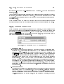
Stuttgart Neural Network Simulator
User Manual, Version 4.2
UNIVERSITY OF STUTTGART
INSTITUTE FOR PARALLEL AND DISTRIBUTED
HIGH PERFORMANCE SYSTEMS (IPVR)
Applied Computer Science { Image Understanding
UNIVERSITY OF TUBINGEN
WILHELM{SCHICKARD{INSTITUTE
FOR COMPUTER SCIENCE
Department of Computer Architecture
UNIVERSITY OF STUTTGART
INSTITUTE FOR PARALLEL AND DISTRIBUTED
HIGH PERFORMANCE SYSTEMS (IPVR)
Applied Computer Science { Image Understanding
UNIVERSITY OF TUBINGEN
WILHELM{SCHICKARD{INSTITUTE
FOR COMPUTER SCIENCE
Department of Computer Architecture
SNNS
Stuttgart Neural Network Simulator
User Manual, Version 4.2
Andreas Zell, G
unter Mamier, Michael Vogt
Niels Mache, Ralf H
ubner, Sven D
oring
Kai-Uwe Herrmann, Tobias Soyez, Michael Schmalzl
Tilman Sommer, Artemis Hatzigeorgiou, Dietmar Posselt
Tobias Schreiner, Bernward Kett, Gianfranco Clemente
Jens Wieland, J
urgen Gatter
external contributions by
Martin Reczko, Martin Riedmiller
Mark Seemann, Marcus Ritt, Jamie DeCoster
Jochen Biedermann, Joachim Danz, Christian Wehrfritz
Randolf Werner, Michael Berthold, Bruno Orsier
All Rights reserved
Contents
1 Introduction to SNNS
1
2 Licensing, Installation and Acknowledgments
4
2.1
2.2
2.3
2.4
2.5
2.6
SNNS License . . . . . . . . .
How to obtain SNNS . . . . .
Installation . . . . . . . . . .
Contact Points . . . . . . . .
Acknowledgments . . . . . . .
New Features of Release 4.2 .
.
.
.
.
.
.
..
..
..
..
..
..
.
.
.
.
.
.
3 Neural Network Terminology
3.1 Building Blocks of Neural Nets . .
3.1.1 Units . . . . . . . . . . . .
3.1.2 Connections (Links) . . . .
3.1.3 Sites . . . . . . . . . . . . .
3.2 Update Modes . . . . . . . . . . .
3.3 Learning in Neural Nets . . . . . .
3.4 Generalization of Neural Networks
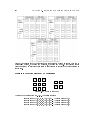
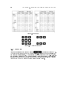
3.5 An Example of a simple Network .
.
.
.
.
.
.
.
.
4 Using the Graphical User Interface
.
.
.
.
.
.
.
.
.
.
.
.
.
.
..
..
..
..
..
..
..
..
..
..
..
..
..
..
.
.
.
.
.
.
.
.
.
.
.
.
.
.
..
..
..
..
..
..
..
..
..
..
..
..
..
..
4.1 Basic SNNS usage . . . . . . . . . . . . . . . .
4.1.1 Startup . . . . . . . . . . . . . . . . . .
4.1.2 Reading and Writing Files . . . . . . . .
4.1.3 Creating New Networks . . . . . . . . .
4.1.4 Training Networks . . . . . . . . . . . .
4.1.4.1 Initialization . . . . . . . . . .
4.1.4.2 Selecting a learning function .
4.1.5 Saving Results for Testing . . . . . . . .
4.1.6 Further Explorations . . . . . . . . . . .
4.1.7 SNNS File Formats . . . . . . . . . . . .
i
.
.
.
.
.
.
.
.
.
.
.
.
.
.
.
.
.
.
.
.
.
.
.
.
..
..
..
..
..
..
..
..
..
..
..
..
..
..
..
..
..
..
..
..
..
..
..
..
.
.
.
.
.
.
.
.
.
.
.
.
.
.
.
.
.
.
.
.
.
.
.
.
.
.
.
.
.
.
.
.
.
.
.
.
.
.
.
.
.
.
.
.
.
.
.
.
..
..
..
..
..
..
..
..
..
..
..
..
..
..
..
..
..
..
..
..
..
..
..
..
.
.
.
.
.
.
.
.
.
.
.
.
.
.
.
.
.
.
.
.
.
.
.
.
..
..
..
..
..
..
..
..
..
..
..
..
..
..
..
..
..
..
..
..
..
..
..
..
.
.
.
.
.
.
.
.
.
.
.
.
.
.
.
.
.
.
.
.
.
.
.
.
.
.
.
.
.
.
.
.
.
.
.
.
.
.
.
.
.
.
.
.
.
.
.
.
..
..
..
..
..
..
..
..
..
..
..
..
..
..
..
..
..
..
..
..
..
..
..
..
.
.
.
.
.
.
.
.
.
.
.
.
.
.
.
.
.
.
.
.
.
.
.
.
.
.
.
.
.
.
.
.
.
.
.
.
.
.
.
.
.
.
.
.
.
.
.
.
5
6
7
11
12
15
18
18
19
23
24
24
25
27
28
29
29
29
30
31
34
34
34
36
36
36
ii
CONTENTS
4.2
4.3
4.4
4.5
4.6
4.7
4.8
4.1.7.1 Pattern les . . . . . . . . . . . . .
4.1.7.2 Network les . . . . . . . . . . . . .
XGUI Files . . . . . . . . . . . . . . . . . . . . . . .
Windows of XGUI . . . . . . . . . . . . . . . . . . .
4.3.1 Manager Panel . . . . . . . . . . . . . . . . .
4.3.2 File Browser . . . . . . . . . . . . . . . . . .
4.3.2.1 Loading and Saving Networks . . .
4.3.2.2 Loading and Saving Patterns . . . .
4.3.2.3 Loading and Saving Congurations
4.3.2.4 Saving a Result le . . . . . . . . .
4.3.2.5 Dening the Log File . . . . . . . .
4.3.3 Control Panel . . . . . . . . . . . . . . . . . .
4.3.4 Info Panel . . . . . . . . . . . . . . . . . . . .
4.3.4.1 Unit Function Displays . . . . . . .
4.3.5 2D Displays . . . . . . . . . . . . . . . . . . .
4.3.5.1 Setup Panel of a 2D Display . . . .
4.3.6 Graph Window . . . . . . . . . . . . . . . . .
4.3.7 Weight Display . . . . . . . . . . . . . . . . .
4.3.8 Projection Panel . . . . . . . . . . . . . . . .
4.3.9 Print Panel . . . . . . . . . . . . . . . . . . .
4.3.10 Class Panel . . . . . . . . . . . . . . . . . . .
4.3.11 Help Windows . . . . . . . . . . . . . . . . .
4.3.12 Shell window . . . . . . . . . . . . . . . . . .
4.3.13 Conrmer . . . . . . . . . . . . . . . . . . . .
Parameters of the Learning Functions . . . . . . . .
Update Functions . . . . . . . . . . . . . . . . . . . .
Initialization Functions . . . . . . . . . . . . . . . . .
Pattern Remapping Functions . . . . . . . . . . . . .
Creating and Editing Unit Prototypes and Sites . . .
5 Handling Patterns with SNNS
5.1
5.2
5.3
5.4
5.5
..
..
..
..
..
..
..
..
..
..
..
..
..
..
..
..
..
..
..
..
..
..
..
..
..
..
..
..
..
.
.
.
.
.
.
.
.
.
.
.
.
.
.
.
.
.
.
.
.
.
.
.
.
.
.
.
.
.
Handling Pattern Sets . . . . . . . . . . . . . . . . . . . .
Fixed Size Patterns . . . . . . . . . . . . . . . . . . . . . .
Variable Size Patterns . . . . . . . . . . . . . . . . . . . .
Patterns with Class Information and Virtual Pattern Sets
Pattern Remapping . . . . . . . . . . . . . . . . . . . . . .
..
..
..
..
..
..
..
..
..
..
..
..
..
..
..
..
..
..
..
..
..
..
..
..
..
..
..
..
..
..
..
..
..
..
.
.
.
.
.
.
.
.
.
.
.
.
.
.
.
.
.
.
.
.
.
.
.
.
.
.
.
.
.
.
.
.
.
.
.
.
.
.
.
.
.
.
.
.
.
.
.
.
.
.
.
.
.
.
.
.
.
.
.
.
.
.
.
.
.
.
.
.
..
..
..
..
..
..
..
..
..
..
..
..
..
..
..
..
..
..
..
..
..
..
..
..
..
..
..
..
..
..
..
..
..
..
.
.
.
.
.
.
.
.
.
.
.
.
.
.
.
.
.
.
.
.
.
.
.
.
.
.
.
.
.
.
.
.
.
.
..
..
..
..
..
..
..
..
..
..
..
..
..
..
..
..
..
..
..
..
..
..
..
..
..
..
..
..
..
..
..
..
..
..
.
.
.
.
.
.
.
.
.
.
.
.
.
.
.
.
.
.
.
.
.
.
.
.
.
.
.
.
.
36
36
37
38
40
41
42
43
43
43
44
44
50
53
54
54
57
58
60
61
62
63
64
66
67
76
82
87
90
92
. 93
. 93
. 93
. 98
. 101
iii
CONTENTS
6 Graphical Network Editor
6.1 Editor Modes . . . . . . . . .
6.2 Selection . . . . . . . . . . . .
6.2.1 Selection of Units . . .
6.2.2 Selection of Links . . .
6.3 Use of the Mouse . . . . . . .
6.4 Short Command Reference .
6.5 Editor Commands . . . . . .
6.6 Example Dialogue . . . . . .
.
.
.
.
.
.
.
.
..
..
..
..
..
..
..
..
7 Graphical Network Creation Tools
.
.
.
.
.
.
.
.
.
.
.
.
.
.
.
.
..
..
..
..
..
..
..
..
.
.
.
.
.
.
.
.
..
..
..
..
..
..
..
..
.
.
.
.
.
.
.
.
..
..
..
..
..
..
..
..
7.1 BigNet for Feed-Forward and Recurrent Networks .
7.1.1 Terminology of the Tool BigNet . . . . . . . .
7.1.2 Buttons of BigNet . . . . . . . . . . . . . . .
7.1.3 Plane Editor . . . . . . . . . . . . . . . . . .
7.1.4 Link Editor . . . . . . . . . . . . . . . . . . .
7.1.5 Create Net . . . . . . . . . . . . . . . . . . .
7.2 BigNet for Time-Delay Networks . . . . . . . . . . .
7.2.1 Terminology of Time-Delay BigNet . . . . . .
7.2.2 Plane Editor . . . . . . . . . . . . . . . . . .
7.2.3 Link Editor . . . . . . . . . . . . . . . . . . .
7.3 BigNet for ART-Networks . . . . . . . . . . . . . . .
7.4 BigNet for Self-Organizing Maps . . . . . . . . . . .
7.5 BigNet for Autoassociative Memory Networks . . . .
7.6 BigNet for Partial Recurrent Networks . . . . . . . .
7.6.1 BigNet for Jordan Networks . . . . . . . . . .
7.6.2 BigNet for Elman Networks . . . . . . . . . .
8 Network Analyzing Tools
.
.
.
.
.
.
.
.
.
.
.
.
.
.
.
.
.
.
.
.
.
.
.
.
.
.
.
.
.
.
.
.
.
.
.
.
.
.
.
.
.
.
.
.
.
.
.
.
..
..
..
..
..
..
..
..
..
..
..
..
..
..
..
..
..
..
..
..
..
..
..
..
.
.
.
.
.
.
.
.
.
.
.
.
.
.
.
.
.
.
.
.
.
.
.
.
..
..
..
..
..
..
..
..
..
..
..
..
..
..
..
..
..
..
..
..
..
..
..
..
8.1 Inversion . . . . . . . . . . . . . . . . . . . . . . . . . . . . . . . .
8.1.1 The Algorithm . . . . . . . . . . . . . . . . . . . . . . . .
8.1.2 Inversion Display . . . . . . . . . . . . . . . . . . . . . . .
8.1.3 Example Session . . . . . . . . . . . . . . . . . . . . . . .
8.2 Network Analyzer . . . . . . . . . . . . . . . . . . . . . . . . . .
8.2.1 The Network Analyzer Setup . . . . . . . . . . . . . . . .
8.2.2 The Display Control Window of the Network Analyzer . .
.
.
.
.
.
.
.
.
.
.
.
.
.
.
.
.
.
.
.
.
.
.
.
.
.
.
.
.
.
.
.
.
.
.
.
.
.
.
.
.
.
.
.
.
.
.
.
.
.
.
.
.
.
.
.
.
.
.
.
.
.
.
..
..
..
..
..
..
..
..
..
..
..
..
..
..
..
..
..
..
..
..
..
..
..
..
..
..
..
..
..
..
..
.
.
.
.
.
.
.
.
.
.
.
.
.
.
.
.
.
.
.
.
.
.
.
.
.
.
.
.
.
.
.
103
. 104
. 104
. 104
. 105
. 105
. 106
. 110
. 117
119
. 119
. 119
. 121
. 123
. 123
. 126
. 127
. 127
. 128
. 128
. 130
. 131
. 132
. 133
. 133
. 134
136
. 136
. 136
. 137
. 139
. 140
. 142
. 144
iv
CONTENTS
9 Neural Network Models and Functions
145
9.1 Backpropagation Networks . . . . . . . . . . . . . . . . . . . . . . . . . . . 145
9.1.1 Vanilla Backpropagation . . . . . . . . . . . . . . . . . . . . . . . . . 145
9.1.2 Enhanced Backpropagation . . . . . . . . . . . . . . . . . . . . . . . 145
9.1.3 Batch Backpropagation . . . . . . . . . . . . . . . . . . . . . . . . . 146
9.1.4 Backpropagation with chunkwise update . . . . . . . . . . . . . . . . 146
9.1.5 Backpropagation with Weight Decay . . . . . . . . . . . . . . . . . . 148
9.2 Quickprop . . . . . . . . . . . . . . . . . . . . . . . . . . . . . . . . . . . . . 148
9.3 RPROP . . . . . . . . . . . . . . . . . . . . . . . . . . . . . . . . . . . . . . 148
9.3.1 Changes in Release 3.3 . . . . . . . . . . . . . . . . . . . . . . . . . . 148
9.3.2 General Description . . . . . . . . . . . . . . . . . . . . . . . . . . . 149
9.3.3 Parameters . . . . . . . . . . . . . . . . . . . . . . . . . . . . . . . . 150
9.4 Rprop with adaptive weight-decay (RpropMAP) . . . . . . . . . . . . . . . 150
9.4.1 Parameters . . . . . . . . . . . . . . . . . . . . . . . . . . . . . . . . 150
9.4.2 Determining the weighting factor . . . . . . . . . . . . . . . . . . . 151
9.5 Backpercolation . . . . . . . . . . . . . . . . . . . . . . . . . . . . . . . . . . 152
9.6 Counterpropagation . . . . . . . . . . . . . . . . . . . . . . . . . . . . . . . 152
9.6.1 Fundamentals . . . . . . . . . . . . . . . . . . . . . . . . . . . . . . . 152
9.6.2 Initializing Counterpropagation . . . . . . . . . . . . . . . . . . . . . 153
9.6.3 Counterpropagation Implementation in SNNS . . . . . . . . . . . . . 154
9.7 Dynamic Learning Vector Quantization (DLVQ) . . . . . . . . . . . . . . . 154
9.7.1 DLVQ Fundamentals . . . . . . . . . . . . . . . . . . . . . . . . . . . 154
9.7.2 DLVQ in SNNS . . . . . . . . . . . . . . . . . . . . . . . . . . . . . . 155
9.7.3 Remarks . . . . . . . . . . . . . . . . . . . . . . . . . . . . . . . . . . 157
9.8 Backpropagation Through Time (BPTT) . . . . . . . . . . . . . . . . . . . 157
9.9 The Cascade Correlation Algorithms . . . . . . . . . . . . . . . . . . . . . . 159
9.9.1 Cascade-Correlation (CC) . . . . . . . . . . . . . . . . . . . . . . . . 160
9.9.1.1 The Algorithm . . . . . . . . . . . . . . . . . . . . . . . . . 160
9.9.1.2 Mathematical Background . . . . . . . . . . . . . . . . . . 160
9.9.2 Modications of Cascade-Correlation . . . . . . . . . . . . . . . . . . 162
9.9.2.1 Sibling/Descendant Cascade-Correlation (SDCC) . . . . . 162
9.9.2.2 Random Layer Cascade Correlation (RLCC) . . . . . . . . 163
9.9.2.3 Static Algorithms . . . . . . . . . . . . . . . . . . . . . . . 163
9.9.2.4 Exponential CC (ECC) . . . . . . . . . . . . . . . . . . . . 163
9.9.2.5 Limited Fan-In Random Wired Cascade Correlation (LFCC)164
9.9.2.6 Grouped Cascade-Correlation (GCC) . . . . . . . . . . . . 164
9.9.2.7 Comparison of the modications . . . . . . . . . . . . . . . 164
v
CONTENTS
9.10
9.11
9.12
9.13
9.14
9.9.3 Pruned-Cascade-Correlation (PCC) . . . . . . . . .
9.9.3.1 The Algorithm . . . . . . . . . . . . . . . .
9.9.3.2 Mathematical Background . . . . . . . . .
9.9.4 Recurrent Cascade-Correlation (RCC) . . . . . . . .
9.9.5 Using the Cascade Algorithms/TACOMA in SNNS .
Time Delay Networks (TDNNs) . . . . . . . . . . . . . . . .
9.10.1 TDNN Fundamentals . . . . . . . . . . . . . . . . .
9.10.2 TDNN Implementation in SNNS . . . . . . . . . . .
9.10.2.1 Activation Function . . . . . . . . . . . . .
9.10.2.2 Update Function . . . . . . . . . . . . . . .
9.10.2.3 Learning Function . . . . . . . . . . . . . .
9.10.3 Building and Using a Time Delay Network . . . . .
Radial Basis Functions (RBFs) . . . . . . . . . . . . . . . .
9.11.1 RBF Fundamentals . . . . . . . . . . . . . . . . . . .
9.11.2 RBF Implementation in SNNS . . . . . . . . . . . .
9.11.2.1 Activation Functions . . . . . . . . . . . .
9.11.2.2 Initialization Functions . . . . . . . . . . .
9.11.2.3 Learning Functions . . . . . . . . . . . . .
9.11.3 Building a Radial Basis Function Application . . . .
Dynamic Decay Adjustment for RBFs (RBF{DDA) . . . .
9.12.1 The Dynamic Decay Adjustment Algorithm . . . . .
9.12.2 Using RBF{DDA in SNNS . . . . . . . . . . . . . .
ART Models in SNNS . . . . . . . . . . . . . . . . . . . . .
9.13.1 ART1 . . . . . . . . . . . . . . . . . . . . . . . . . .
9.13.1.1 Structure of an ART1 Network . . . . . . .
9.13.1.2 Using ART1 Networks in SNNS . . . . . .
9.13.2 ART2 . . . . . . . . . . . . . . . . . . . . . . . . . .
9.13.2.1 Structure of an ART2 Network . . . . . . .
9.13.2.2 Using ART2 Networks in SNNS . . . . . .
9.13.3 ARTMAP . . . . . . . . . . . . . . . . . . . . . . . .
9.13.3.1 Structure of an ARTMAP Network . . . .
9.13.3.2 Using ARTMAP Networks in SNNS . . . .
9.13.4 Topology of ART Networks in SNNS . . . . . . . . .
Self-Organizing Maps (SOMs) . . . . . . . . . . . . . . . . .
9.14.1 SOM Fundamentals . . . . . . . . . . . . . . . . . .
9.14.2 SOM Implementation in SNNS . . . . . . . . . . . .
9.14.2.1 The KOHONEN Learning Function . . . .
9.14.2.2 The Kohonen Update Function . . . . . . .
.
.
.
.
.
.
.
.
.
.
.
.
.
.
.
.
.
.
.
.
.
.
.
.
.
.
.
.
.
.
.
.
.
.
.
.
.
.
..
..
..
..
..
..
..
..
..
..
..
..
..
..
..
..
..
..
..
..
..
..
..
..
..
..
..
..
..
..
..
..
..
..
..
..
..
..
.
.
.
.
.
.
.
.
.
.
.
.
.
.
.
.
.
.
.
.
.
.
.
.
.
.
.
.
.
.
.
.
.
.
.
.
.
.
.
.
.
.
.
.
.
.
.
.
.
.
.
.
.
.
.
.
.
.
.
.
.
.
.
.
.
.
.
.
.
.
.
.
.
.
.
.
..
..
..
..
..
..
..
..
..
..
..
..
..
..
..
..
..
..
..
..
..
..
..
..
..
..
..
..
..
..
..
..
..
..
..
..
..
..
.
.
.
.
.
.
.
.
.
.
.
.
.
.
.
.
.
.
.
.
.
.
.
.
.
.
.
.
.
.
.
.
.
.
.
.
.
.
. 165
. 165
. 165
. 165
. 166
. 169
. 169
. 170
. 171
. 171
. 171
. 171
. 172
. 172
. 175
. 175
. 176
. 180
. 181
. 183
. 183
. 186
. 187
. 188
. 188
. 189
. 190
. 190
. 191
. 193
. 193
. 194
. 195
. 198
. 198
. 199
. 199
. 200
vi
CONTENTS
9.15
9.16
9.17
9.18
9.19
9.14.2.3 The Kohonen Init Function . . . . . . . . . .
9.14.2.4 The Kohonen Activation Functions . . . . .
9.14.2.5 Building and Training Self-Organizing Maps
9.14.2.6 Evaluation Tools for SOMs . . . . . . . . . .
Autoassociative Networks . . . . . . . . . . . . . . . . . . . .
9.15.1 General Characteristics . . . . . . . . . . . . . . . . .
9.15.2 Layout of Autoassociative Networks . . . . . . . . . .
9.15.3 Hebbian Learning . . . . . . . . . . . . . . . . . . . .
9.15.4 McClelland & Rumelhart's Delta Rule . . . . . . . . .
Partial Recurrent Networks . . . . . . . . . . . . . . . . . . .
9.16.1 Models of Partial Recurrent Networks . . . . . . . . .
9.16.1.1 Jordan Networks . . . . . . . . . . . . . . . .
9.16.1.2 Elman Networks . . . . . . . . . . . . . . . .
9.16.1.3 Extended Hierarchical Elman Networks . . .
9.16.2 Working with Partial Recurrent Networks . . . . . . .
9.16.2.1 The Initialization Function JE Weights . . .
9.16.2.2 Learning Functions . . . . . . . . . . . . . .
9.16.2.3 Update Functions . . . . . . . . . . . . . . .
Stochastic Learning Functions . . . . . . . . . . . . . . . . . .
9.17.1 Monte-Carlo . . . . . . . . . . . . . . . . . . . . . . .
9.17.2 Simulated Annealing . . . . . . . . . . . . . . . . . . .
Scaled Conjugate Gradient (SCG) . . . . . . . . . . . . . . .
9.18.1 Conjugate Gradient Methods (CGMs) . . . . . . . . .
9.18.2 Main features of SCG . . . . . . . . . . . . . . . . . .
9.18.3 Parameters of SCG . . . . . . . . . . . . . . . . . . . .
9.18.4 Complexity of SCG . . . . . . . . . . . . . . . . . . .
TACOMA Learning . . . . . . . . . . . . . . . . . . . . . . .
9.19.1 Overview . . . . . . . . . . . . . . . . . . . . . . . . .
9.19.2 The algorithm in detail . . . . . . . . . . . . . . . . .
9.19.3 Advantages/Disadvantages TACOMA . . . . . . . . .
10 Pruning Algorithms
10.1 Background of Pruning Algorithms . .
10.2 Theory of the implemented algorithms
10.2.1 Magnitude Based Pruning . . .
10.2.2 Optimal Brain Damage . . . .
10.2.3 Optimal Brain Surgeon . . . .
10.2.4 Skeletonization . . . . . . . . .
10.2.5 Non-contributing Units . . . .
.
.
.
.
.
.
.
..
..
..
..
..
..
..
.
.
.
.
.
.
.
.
.
.
.
.
.
.
..
..
..
..
..
..
..
.
.
.
.
.
.
.
..
..
..
..
..
..
..
.
.
.
.
.
.
.
..
..
..
..
..
..
..
.
.
.
.
.
.
.
.
.
.
.
.
.
.
.
.
.
.
.
.
.
.
.
.
.
.
.
.
.
.
.
.
.
.
.
.
.
.
.
.
.
.
.
.
.
.
.
.
.
.
.
.
.
.
.
.
.
.
.
.
.
.
.
.
.
.
.
.
.
.
.
.
.
.
..
..
..
..
..
..
..
..
..
..
..
..
..
..
..
..
..
..
..
..
..
..
..
..
..
..
..
..
..
..
..
..
..
..
..
..
..
.
.
.
.
.
.
.
.
.
.
.
.
.
.
.
.
.
.
.
.
.
.
.
.
.
.
.
.
.
.
.
.
.
.
.
.
.
..
..
..
..
..
..
..
..
..
..
..
..
..
..
..
..
..
..
..
..
..
..
..
..
..
..
..
..
..
..
..
..
..
..
..
..
..
. 200
. 200
. 200
. 201
. 202
. 202
. 202
. 203
. 204
. 205
. 205
. 205
. 205
. 206
. 206
. 207
. 207
. 208
. 208
. 209
. 209
. 209
. 210
. 210
. 211
. 211
. 212
. 212
. 212
. 215
216
. 216
. 217
. 217
. 217
. 218
. 218
. 219
vii
CONTENTS
10.3 Pruning Nets in SNNS . . . . . . . . . . . . . . . . . . . . . . . . . . . . . . 219
11 3D-Visualization of Neural Networks
11.1 Overview of the 3D Network Visualization . . . . . . . . . .
11.2 Use of the 3D-Interface . . . . . . . . . . . . . . . . . . . . .
11.2.1 Structure of the 3D-Interface . . . . . . . . . . . . .
11.2.2 Calling and Leaving the 3D Interface . . . . . . . . .
11.2.3 Creating a 3D-Network . . . . . . . . . . . . . . . .
11.2.3.1 Concepts . . . . . . . . . . . . . . . . . . .
11.2.3.2 Assigning a new z-Coordinate . . . . . . .
11.2.3.3 Moving a z-Plane . . . . . . . . . . . . . .
11.2.3.4 Displaying the z-Coordinates . . . . . . . .
11.2.3.5 Example Dialogue to Create a 3D-Network
11.2.4 3D-Control Panel . . . . . . . . . . . . . . . . . . . .
11.2.4.1 Transformation Panels . . . . . . . . . . . .
11.2.4.2 Setup Panel . . . . . . . . . . . . . . . . .
11.2.4.3 Model Panel . . . . . . . . . . . . . . . . .
11.2.4.4 Project Panel . . . . . . . . . . . . . . . . .
11.2.4.5 Light Panel . . . . . . . . . . . . . . . . . .
11.2.4.6 Unit Panel . . . . . . . . . . . . . . . . . .
11.2.4.7 Links Panel . . . . . . . . . . . . . . . . . .
11.2.4.8 Reset Button . . . . . . . . . . . . . . . . .
11.2.4.9 Freeze Button . . . . . . . . . . . . . . . .
11.2.5 3D-Display Window . . . . . . . . . . . . . . . . . .
12 Batchman
12.1 Introduction . . . . . . . . . . . . . . . . . . . . .
12.1.1 Styling Conventions . . . . . . . . . . . .
12.1.2 Calling the Batch Interpreter . . . . . . .
12.2 Description of the Batch Language . . . . . . . .
12.2.1 Structure of a Batch Program . . . . . . .
12.2.2 Data Types and Variables . . . . . . . . .
12.2.3 Variables . . . . . . . . . . . . . . . . . .
12.2.4 System Variables . . . . . . . . . . . . . .
12.2.5 Operators and Expressions . . . . . . . .
12.2.6 The Print Function . . . . . . . . . . . . .
12.2.7 Control Structures . . . . . . . . . . . . .
12.3 SNNS Function Calls . . . . . . . . . . . . . . . .
12.3.1 Function Calls To Set SNNS Parameters .
12.3.2 Function Calls Related To Networks . . .
..
..
..
..
..
..
..
..
..
..
..
..
..
..
.
.
.
.
.
.
.
.
.
.
.
.
.
.
.
.
.
.
.
.
.
.
.
.
.
.
.
.
..
..
..
..
..
..
..
..
..
..
..
..
..
..
.
.
.
.
.
.
.
.
.
.
.
.
.
.
.
.
.
.
.
.
.
.
.
.
.
.
.
.
.
.
.
.
.
.
.
..
..
..
..
..
..
..
..
..
..
..
..
..
..
..
..
..
..
..
..
..
..
..
..
..
..
..
..
..
..
..
..
..
..
..
.
.
.
.
.
.
.
.
.
.
.
.
.
.
.
.
.
.
.
.
.
.
.
.
.
.
.
.
.
.
.
.
.
.
.
.
.
.
.
.
.
.
.
.
.
.
.
.
.
.
.
.
.
.
.
.
.
.
.
.
.
.
.
.
.
.
.
.
.
.
..
..
..
..
..
..
..
..
..
..
..
..
..
..
..
..
..
..
..
..
..
..
..
..
..
..
..
..
..
..
..
..
..
..
..
.
.
.
.
.
.
.
.
.
.
.
.
.
.
.
.
.
.
.
.
.
.
.
.
.
.
.
.
.
.
.
.
.
.
.
222
. 222
. 223
. 223
. 223
. 223
. 223
. 224
. 225
. 225
. 225
. 227
. 229
. 230
. 230
. 231
. 231
. 232
. 233
. 233
. 233
. 233
235
. 235
. 235
. 236
. 237
. 237
. 238
. 238
. 239
. 239
. 241
. 241
. 243
. 245
. 252
viii
CONTENTS
12.3.3 Pattern Function Calls . . .
12.3.4 Special Functions . . . . . .
12.4 Batchman Example Programs . . .
12.4.1 Example 1 . . . . . . . . . .
12.4.2 Example 2 . . . . . . . . . .
12.4.3 Example 3 . . . . . . . . . .
12.5 Snnsbat { The predessor . . . . . .
12.5.1 The Snnsbat Environment .
12.5.2 Using Snnsbat . . . . . . .
12.5.3 Calling Snnsbat . . . . . . .
.
.
.
.
.
.
.
.
.
.
..
..
..
..
..
..
..
..
..
..
.
.
.
.
.
.
.
.
.
.
..
..
..
..
..
..
..
..
..
..
. 255
. 256
. 258
. 258
. 259
. 260
. 261
. 261
. 261
. 267
13.1 Overview . . . . . . . . . . . . . . . . . . . . . . . . . . . . . . .
13.2 Analyze . . . . . . . . . . . . . . . . . . . . . . . . . . . . . . . .
13.2.1 Analyzing Functions . . . . . . . . . . . . . . . . . . . . .
13.3 bignet . . . . . . . . . . . . . . . . . . . . . . . . . . . . . . . .
13.4 td bignet . . . . . . . . . . . . . . . . . . . . . . . . . . . . . . .
13.5 linknets . . . . . . . . . . . . . . . . . . . . . . . . . . . . . . . .
13.5.1 Limitations . . . . . . . . . . . . . . . . . . . . . . . . . .
13.5.2 Notes on further training . . . . . . . . . . . . . . . . . .
13.5.3 Examples . . . . . . . . . . . . . . . . . . . . . . . . . . .
13.6 Convert2snns . . . . . . . . . . . . . . . . . . . . . . . . . . . . .
13.6.1 Setup and Structure of a Control, Weight, Pattern File .
13.7 Feedback-gennet . . . . . . . . . . . . . . . . . . . . . . . . . . .
13.8 Mkhead . . . . . . . . . . . . . . . . . . . . . . . . . . . . . . . .
13.9 Mkout . . . . . . . . . . . . . . . . . . . . . . . . . . . . . . . . .
13.10Mkpat . . . . . . . . . . . . . . . . . . . . . . . . . . . . . . . . .
13.11Netlearn . . . . . . . . . . . . . . . . . . . . . . . . . . . . . . . .
13.12Netperf . . . . . . . . . . . . . . . . . . . . . . . . . . . . . . . .
13.13Pat sel . . . . . . . . . . . . . . . . . . . . . . . . . . . . . . . . .
13.14Snns2c . . . . . . . . . . . . . . . . . . . . . . . . . . . . . . . . .
13.14.1 Program Flow . . . . . . . . . . . . . . . . . . . . . . . .
13.14.2 Including the Compiled Network in the Own Application
13.14.3 Special Network Architectures . . . . . . . . . . . . . . .
13.14.4 Activation Functions . . . . . . . . . . . . . . . . . . . . .
13.14.5 Error Messages . . . . . . . . . . . . . . . . . . . . . . . .
13.15isnns . . . . . . . . . . . . . . . . . . . . . . . . . . . . . . . . . .
13.15.1 Commands . . . . . . . . . . . . . . . . . . . . . . . . . .
13.15.2 Example . . . . . . . . . . . . . . . . . . . . . . . . . . . .
..
..
..
..
..
..
..
..
..
..
..
..
..
..
..
..
..
..
..
..
..
..
..
..
..
..
..
.
.
.
.
.
.
.
.
.
.
.
.
.
.
.
.
.
.
.
.
.
.
.
.
.
.
.
..
..
..
..
..
..
..
..
..
..
..
..
..
..
..
..
..
..
..
..
..
..
..
..
..
..
..
. 268
. 268
. 269
. 270
. 272
. 272
. 274
. 274
. 275
. 276
. 277
. 277
. 278
. 278
. 278
. 279
. 280
. 281
. 281
. 282
. 283
. 284
. 284
. 285
. 286
. 286
. 288
13 Tools for SNNS
..
..
..
..
..
..
..
..
..
..
.
.
.
.
.
.
.
.
.
.
..
..
..
..
..
..
..
..
..
..
.
.
.
.
.
.
.
.
.
.
.
.
.
.
.
.
.
.
.
.
..
..
..
..
..
..
..
..
..
..
.
.
.
.
.
.
.
.
.
.
..
..
..
..
..
..
..
..
..
..
.
.
.
.
.
.
.
.
.
.
..
..
..
..
..
..
..
..
..
..
.
.
.
.
.
.
.
.
.
.
268
ix
CONTENTS
14 Kernel Function Interface
14.1 Overview . . . . . . . . . . . . . . . . . . . . . . . . .
14.2 Unit Functions . . . . . . . . . . . . . . . . . . . . . .
14.3 Site Functions . . . . . . . . . . . . . . . . . . . . . . .
14.4 Link Functions . . . . . . . . . . . . . . . . . . . . . .
14.5 Functions for the Manipulation of Prototypes . . . . .
14.6 Functions to Read the Function Table . . . . . . . . .
14.7 Network Initialization Functions . . . . . . . . . . . .
14.8 Functions for Activation Propagation in the Network .
14.9 Learning and Pruning Functions . . . . . . . . . . . .
14.10Functions for the Manipulation of Patterns . . . . . .
14.11File I/O Functions . . . . . . . . . . . . . . . . . . . .
14.12Functions to Search the Symbol Table . . . . . . . . .
14.13Miscelaneous other Interface Functions . . . . . . . . .
14.14Memory Management Functions . . . . . . . . . . . .
14.15ART Interface Functions . . . . . . . . . . . . . . . . .
14.16Error Messages of the Simulator Kernel . . . . . . . .
.
.
.
.
.
.
.
.
.
.
.
.
.
.
.
.
..
..
..
..
..
..
..
..
..
..
..
..
..
..
..
..
.
.
.
.
.
.
.
.
.
.
.
.
.
.
.
.
..
..
..
..
..
..
..
..
..
..
..
..
..
..
..
..
.
.
.
.
.
.
.
.
.
.
.
.
.
.
.
.
.
.
.
.
.
.
.
.
.
.
.
.
.
.
.
.
..
..
..
..
..
..
..
..
..
..
..
..
..
..
..
..
.
.
.
.
.
.
.
.
.
.
.
.
.
.
.
.
15 Transfer Functions
290
. 290
. 290
. 296
. 298
. 300
. 302
. 302
. 303
. 304
. 305
. 308
. 308
. 309
. 309
. 310
. 311
315
15.1 Predened Transfer Functions . . . . . . . . . . . . . . . . . . . . . . . . . . 315
15.2 User Dened Transfer Functions . . . . . . . . . . . . . . . . . . . . . . . . 318
A Kernel File Interface
A.1 The ASCII Network File Format . . . . . . . . . . .
A.2 Form of the Network File Entries . . . . . . . . . . .
A.3 Grammar of the Network Files . . . . . . . . . . . .
A.3.1 Conventions . . . . . . . . . . . . . . . . . . .
A.3.1.1 Lexical Elements of the Grammar .
A.3.1.2 Denition of the Grammar . . . . .
A.3.2 Terminal Symbols . . . . . . . . . . . . . . .
A.3.3 Grammar: . . . . . . . . . . . . . . . . . . . .
A.4 Grammar of the Pattern Files . . . . . . . . . . . . .
A.4.1 Terminal Symbols . . . . . . . . . . . . . . .
A.4.2 Grammar . . . . . . . . . . . . . . . . . . . .
B Example Network Files
.
.
.
.
.
.
.
.
.
.
.
.
.
.
.
.
.
.
.
.
.
.
..
..
..
..
..
..
..
..
..
..
..
.
.
.
.
.
.
.
.
.
.
.
..
..
..
..
..
..
..
..
..
..
..
.
.
.
.
.
.
.
.
.
.
.
.
.
.
.
.
.
.
.
.
.
.
..
..
..
..
..
..
..
..
..
..
..
.
.
.
.
.
.
.
.
.
.
.
319
. 319
. 320
. 321
. 321
. 321
. 321
. 322
. 323
. 326
. 326
. 326
328
B.1 Example 1: . . . . . . . . . . . . . . . . . . . . . . . . . . . . . . . . . . . . 328
B.2 Example 2: . . . . . . . . . . . . . . . . . . . . . . . . . . . . . . . . . . . . 331
[This page intentionally left blank]
Chapter 1
Introduction to SNNS
SNNS (Stuttgart Neural Network Simulator) is a simulator for neural networks developed
at the Institute for Parallel and Distributed High Performance Systems (Institut fur Parallele und Verteilte Hochstleistungsrechner, IPVR) at the University of Stuttgart since
1989. The goal of the project is to create an eÆcient and exible simulation environment
for research on and application of neural nets.
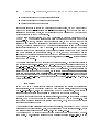
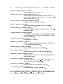
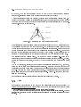
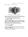
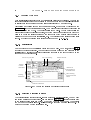
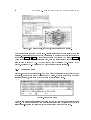
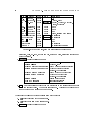
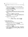
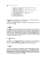
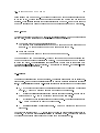
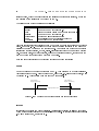
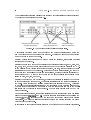
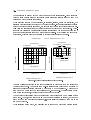
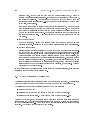
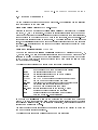
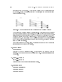
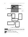
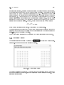
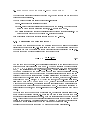
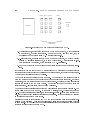
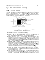
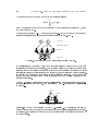
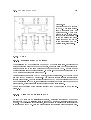
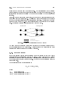
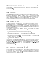
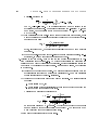
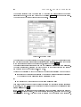
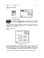
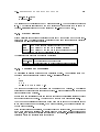
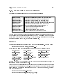
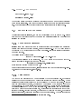
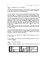
The SNNS simulator consists of four main components that are depicted in gure 1.1:
Simulator kernel, graphical user interface, batch execution interface batchman, and network compiler snns2c. There was also a fth part, Nessus, that was used to construct
networks for SNNS. Nessus, however, has become obsolete since the introduction of powerful interactive network creation tools within the graphical user interface and is no longer
supported. The simulator kernel operates on the internal network data structures of the
neural nets and performs all operations on them. The graphical user interface XGUI1 ,
built on top of the kernel, gives a graphical representation of the neural networks and
controls the kernel during the simulation run. In addition, the user interface can be used
to directly create, manipulate and visualize neural nets in various ways. Complex networks can be created quickly and easily. Nevertheless, XGUI should also be well suited
for unexperienced users, who want to learn about connectionist models with the help of
the simulator. An online help system, partly context-sensitive, is integrated, which can
oer assistance with problems.
An important design concept was to enable the user to select only those aspects of the
visual representation of the net in which he is interested. This includes depicting several
aspects and parts of the network with multiple windows as well as suppressing unwanted
information.
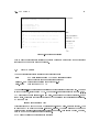
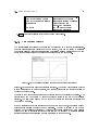
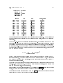
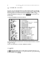
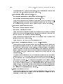
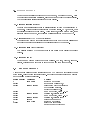
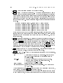
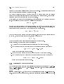
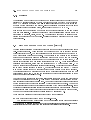
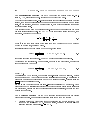
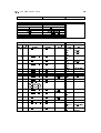
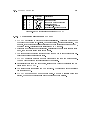
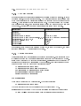
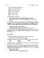
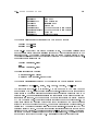
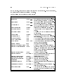
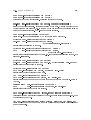
SNNS is implemented completely in ANSI-C. The simulator kernel has already been tested
on numerous machines and operating systems (see also table 1.1). XGUI is based upon
X11 Release 5 from MIT and the Athena Toolkit, and was tested under various window
managers, like twm, tvtwm, olwm, ctwm, fvwm. It also works under X11R6.
1
X Graphical User Interface
2
CHAPTER 1. INTRODUCTION TO SNNS
main()
trained
network file
as C source code
X-Windows
graphical
user interface
XGUI
SNNS 2 C
graphical network
representation
network editor
simulation control
ASCII network
description file
(intermediate
form)
batch execution
script
BATCHMAN
direct
manpulation
user defined
activation
functions
kernel-compiler
file interface
SNNS
simulator
kernel
written in C
activation
functions
kernel-XGUI
function interface
user defined
learning
procedures
learning
procedures
network modification functions
SNNS memory management
internal
network
representation
Unix memory management
Figure 1.1: SNNS components: simulator kernel, graphical user interface xgui, batchman,
and network compiler snns2c
machine type
operating system
SUN SparcSt. ELC,IPC
SunOS 4.1.2, 4.1.3, 5.3, 5.4
SUN SparcSt. 2
SunOS 4.1.2
SUN SparcSt. 5, 10, 20
SunOS 4.1.3, 5.3, 5.4, 5.5
DECstation 3100, 5000
Ultrix V4.2
DEC Alpha AXP 3000
OSF1 V2.1 - V4.0
IBM-PC 80486, Pentium
Linux, NeXTStep
IBM RS 6000/320, 320H, 530H AIX V3.1, AIX V3.2, AIX V4.1
HP 9000/720, 730
HP-UX 8.07, NeXTStep
SGI Indigo 2
IRIX 4.0.5, 5.3, 6.2
NeXTStation
NeXTStep
Table 1.1: Machines and operating systems on which SNNS has been tested
(as of March 1998)
3
This document is structured as follows:
This chapter 1 gives a brief introduction and overview of SNNS.
Chapter 2 gives the details about how to obtain SNNS and under what conditions. It
includes licensing, copying and exclusion of warranty. It then discusses how to install
SNNS and gives acknowledgments of its numerous authors.
Chapter 3 introduces the components of neural nets and the terminology used in the
description of the simulator. Therefore, this chapter may also be of interest to people
already familiar with neural nets.
Chapter 4 describes how to operate the two-dimensional graphical user interface. After a
short overview of all commands a more detailed description of these commands with an
example dialog is given.
Chapter 5 describes the form and usage of the patterns of SNNS
Chapter 6 describes the integrated graphical editor of the 2D user interface. These editor
commands allow the interactive construction of networks with arbitrary topologies.
Chapter 7 is about a tool to facilitate the generation of large, regular networks from the
graphical user interface.
Chapter 8 describes the network analyzing facilities, built into SNNS.
Chapter 9 describes the connectionist models that are already implemented in SNNS, with
a strong emphasis on the less familiar network models.
Chapter 10 describes the pruning functions which are available in SNNS.
Chapter 11 introduces a visualization component for three-dimensional visualization of
the topology and the activity of neural networks with wireframe or solid models.
Chapter 12 introduces the batch capabilities of SNNS. They can be accessed via an additional interface to the kernel, that allows for easy background execution.
Chapter 13 gives a brief overlook over the tools that come with SNNS, without being an
internal part of it.
Chapter 14 describes in detail the interface between the kernel and the graphical user
interface. This function interface is important, since the kernel can be included in user
written C programs.
Chapter 15 details the activation functions and output function that are already built in.
In appendix A the format of the le interface to the kernel is described, in which the nets
are read in and written out by the kernel. Files in this format may also be generated by
any other program, or even an editor.
The grammars for both network and pattern les are also given here.
In appendix B and C examples for network and batch conguration les are given.
Chapter 2
Licensing, Installation and
Acknowledgments
SNNS is c (Copyright) 1990-96 SNNS Group, Institute for Parallel and Distributed HighPerformance Systems (IPVR), University of Stuttgart, Breitwiesenstrasse 20-22, 70565
Stuttgart, Germany, and c (Copyright) 1996-98 SNNS Group, Wilhelm Schickard Institute
for Computer Science, University of Tubingen, Kostlinstr. 6, 72074 Tubingen, Germany.
SNNS is distributed by the University of Tubingen as `Free Software' in a licensing agreement similar in some aspects to the GNU General Public License. There are a number of
important dierences, however, regarding modications and distribution of SNNS to third
parties. Note also that SNNS is not part of the GNU software nor is any of its authors
connected with the Free Software Foundation. We only share some common beliefs about
software distribution. Note further that SNNS is NOT PUBLIC DOMAIN.
The SNNS License is designed to make sure that you have the freedom to give away
verbatim copies of SNNS, that you receive source code or can get it if you want it and
that you can change the software for your personal use; and that you know you can do
these things.
We protect your and our rights with two steps: (1) copyright the software, and (2) oer
you this license which gives you legal permission to copy and distribute the unmodied
software or modify it for your own purpose.
In contrast to the GNU license we do not allow modied copies of our software to be
distributed. You may, however, distribute your modications as separate les (e. g. patch
les) along with our unmodied SNNS software. We encourage users to send changes and
improvements which would benet many other users to us so that all users may receive
these improvements in a later version. The restriction not to distribute modied copies is
also useful to prevent bug reports from someone else's modications.
Also, for our protection, we want to make certain that everyone understands that there is
NO WARRANTY OF ANY KIND for the SNNS software.
2.1. SNNS LICENSE
5
2.1 SNNS License
1. This License Agreement applies to the SNNS program and all accompanying programs and les that are distributed with a notice placed by the copyright holder
saying it may be distributed under the terms of the SNNS License. \SNNS", below,
refers to any such program or work, and a \work based on SNNS" means either
SNNS or any work containing SNNS or a portion of it, either verbatim or with
modications. Each licensee is addressed as \you".
2. You may copy and distribute verbatim copies of SNNS's source code as you receive
it, in any medium, provided that you conspicuously and appropriately publish on
each copy an appropriate copyright notice and disclaimer of warranty; keep intact
all the notices that refer to this License and to the absence of any warranty; and
give any other recipients of SNNS a copy of this license along with SNNS.
3. You may modify your copy or copies of SNNS or any portion of it only for your own
use. You may not distribute modied copies of SNNS. You may, however, distribute
your modications as separate les (e. g. patch les) along with the unmodied SNNS
software. We also encourage users to send changes and improvements which would
benet many other users to us so that all users may receive these improvements in
a later version. The restriction not to distribute modied copies is also useful to
prevent bug reports from someone else's modications.
4. If you distribute copies of SNNS you may not charge anything except the cost for
the media and a fair estimate of the costs of computer time or network time directly
attributable to the copying.
5. You may not copy, modify, sub-license, distribute or transfer SNNS except as expressly provided under this License. Any attempt otherwise to copy, modify, sublicense, distribute or transfer SNNS is void, and will automatically terminate your
rights to use SNNS under this License. However, parties who have received copies,
or rights to use copies, from you under this License will not have their licenses
terminated so long as such parties remain in full compliance.
6. By copying, distributing or modifying SNNS (or any work based on SNNS) you
indicate your acceptance of this license to do so, and all its terms and conditions.
7. Each time you redistribute SNNS (or any work based on SNNS), the recipient automatically receives a license from the original licensor to copy, distribute or modify
SNNS subject to these terms and conditions. You may not impose any further
restrictions on the recipients' exercise of the rights granted herein.
8. Incorporation of SNNS or parts of it in commercial programs requires a special
agreement between the copyright holder and the Licensee in writing and usually
involves the payment of license fees. If you want to incorporate SNNS or parts of it
in commercial programs write to the author about further details.
9. Because SNNS is licensed free of charge, there is no warranty for SNNS, to the
extent permitted by applicable law. The copyright holders and/or other parties
provide SNNS \as is" without warranty of any kind, either expressed or implied,
6
CHAPTER 2. LICENSING, INSTALLATION AND ACKNOWLEDGMENTS
including, but not limited to, the implied warranties of merchantability and tness
for a particular purpose. The entire risk as to the quality and performance of SNNS
is with you. Should the program prove defective, you assume the cost of all necessary
servicing, repair or correction.
10. In no event will any copyright holder, or any other party who may redistribute SNNS
as permitted above, be liable to you for damages, including any general, special,
incidental or consequential damages arising out of the use or inability to use SNNS
(including but not limited to loss of data or data being rendered inaccurate or losses
sustained by you or third parties or a failure of SNNS to operate with any other
programs), even if such holder or other party has been advised of the possibility of
such damages.
2.2 How to obtain SNNS
The SNNS simulator can be obtained via anonymous ftp from host
ftp.informatik.uni-tuebingen.de (134.2.12.18)
in the subdirectory
/pub/SNNS
as le
SNNSv4.2.tar.gz
or in several parts as les
SNNSv4.2.tar.gz.aa, SNNSv4.2.tar.gz.ab, ...
These split les are each less than 1 MB and can be joined with the Unix `cat' command
into one le SNNSv4.2.tar.gz. Be sure to set the ftp mode to binary before transmission
of the les. Also watch out for possible higher version numbers, patches or Readme les
in the above directory /pub/SNNS. After successful transmission of the le move it to the
directory where you want to install SNNS, unzip and untar the le with the Unix command
unzip SNNSv4.2.tar.gz
j
tar xvf -
This will extract SNNS in the current directory. The SNNS distribution includes full
source code, installation procedures for supported machine architectures and some simple
examples of trained networks. The full English documentation as LATEX source code with
PostScript images included and a PostScript version of the documentation is also available
in the SNNS directory.
2.3. INSTALLATION
7
2.3 Installation
Note, that SNNS has not been tested extensively in dierent computer environments and
is a research tool with frequent substantial changes. It should be obvious that we don't
guarantee anything. We are also not staed to answer problems with SNNS or to x bugs
quickly.
SNNS currently runs on color or black and white screens of almost any Unix system, while
the graphical user interface might give problems with systems which are not fully X11R5
(or X11R6) compatible.
For the most impatient reader, the easiest way to compile SNNS is to call
make
in the SNNS root directory.
This should work on most UNIX systems and will compile all necessary programms, but
will not install them. (it keeps them in the corresponding source directories).
For proper installation we do recommend the follwing approach:
Conguring the SNNS Installation
To build and install SNNS in the directory in which you have unpacked the tar le (from
now on called <SNNSDIR>), you rst have to generate the correct Makeles for your
machine architecture and window system used. To do this, simply call the shell script
congure
This makes you ready to install SNNS and its tools in the common SNNS installation
directories <SNNSDIR>/tools/bin/<HOST>, and <SNNSDIR>/xgui/bin/<HOST>.
<HOST> denotes an automatically determined system identication (e.g. alpha-decosf4.0), which is used to install SNNS for dierent hardware and software architectures
within the same directory tree.
If you plan to install SNNS, or parts of it, in a more global place like /usr/local or
/home/yourname you should use the ag --enable-global, optionally combined with the
ag --prefix. Please note that --prefix alone will not work, although it is mentioned
in the usage information for \congure". If you use --enable-global alone, --prefix is
set to /usr/local by default. Using --enable-global will install all binaries of SNNS
into the bin directory below the path dened by --prefix:
configure
-> will install to <SNNSDIR>/[tools|xgui]/bin/<HOST>
configure --enable-global
-> will install to /usr/local/bin
configure --enable-global --prefix /home/yourdir
8
CHAPTER 2. LICENSING, INSTALLATION AND ACKNOWLEDGMENTS
-> will install to /home/yourdir/bin
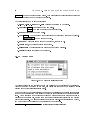
Running \congure" will check your system for the availability of some software tools,
system calls, header les, and X libraries. Also the le cong.h, which is included by most
of the SNNS modules, is created from conguration/cong.hin.
By default, \congure" tries to use the GNU C-compiler gcc, if it is installed on your system. Otherwise cc is used, which must be an ANSI C-compiler. We strongly recommend
to use gcc. However, if you would rather like to use cc or any other C-compiler instead
of an installed gcc, you must set the environment variable CC before running \congure". You may also overwrite the default optimization and debuging ags by dening the
environment variable CFLAGS. Example:
setenv CC acc
setenv CFLAGS -O
configure
There are some useful options for \congure". You will get a short help message, if
you apply the ag --help. Most of the options you will see won't work, because the
SNNS installation directories are determined by other rules as noted in the help message.
However there are some very useful options, which might be of interest. Here is a summary
of all applicable options for \congure"
--quiet
--enable-enzo
--enable-global
--prefix
--x-includes
--x-libraries
--no-create
suppress most of the configuration messages
include all the hookup points in the SNNS kernel
to allow for a later combination with the
genetic algorithm tool ENZO
use global installation path --prefix
path for global installation
alternative path for X include files
alternative path for X libraries
test run, don't change any output files
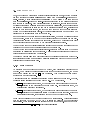
Making and Installing SNNS
After conguring, the next step to build SNNS is usually to make and install the kernel,
the tools and the graphical user interface. This is most easily done with the command
make install
given in the base directory where you have run \congure". This command will descent
into all parts of SNNS to compile and install all necessary parts.
Note:
If you do not install SNNS globally, you should add \<SNNSDIR>/man" to your MANPATH variable if you wish to be able to access the SNNS manpages.
If you want to compile only and refrain from any installation, you may use:
make compile
9
2.3. INSTALLATION
After installing SNNS you may want to cleanup the source directories (delete all object
and library les) with the command
make clean
If you are totally unhappy with your SNNS installation, you can run the command
make uninstall
If you want to compile and install, clean, or uninstall only parts of SNNS, you may also
call one or more of the following commands:
make compile-kernel
make compile-tools
make compile-xgui
(implies making of kernel libraries)
(implies making of kernel libraries)
make install-tools
make install-xgui
(implies making of kernel libraries)
(implies making of kernel libraries)
make clean-kernel
make clean-tools
make clean-xgui
make uninstall-kernel
make uninstall-tools
make uninstall-xgui
If you are a developer and like to modify SNNS or parts of it for your own purpose, there
are even more make targets available for the Makeles in each of the source directories.
See the source of those Makeles for details. Developers experiencing diÆculties may also
nd the target
make bugreport
useful. Please send those reports to the contact address given below.
Note, that SNNS is ready to work together with the genetic algortihm tool ENZO. A
default installation will, however, not support this. If you plan to use genetic algorithms,
you must specify --enable-enzo for the congure call and then later on compile ENZO
in its respective directory. See the ENZO Readme-le and manual for details.
Possible Problems during conguration and compilation of SNNS
\congure" tries to locate all of the tools which might be necessary for the development of
SNNS. However, you don't need to have all of them installed on your system if you only
want to install the unchanged SNNS distribution. You may ignore the following warning
messages but you should keep them in mind whenever you plan to modify SNNS:
10
CHAPTER 2. LICENSING, INSTALLATION AND ACKNOWLEDGMENTS
messages concerning the parser generator 'bison'
messages concerning the scanner generator 'ex'
messages concerning 'makedepend'
If congure is unable to locate the X libraries and include les, you may give advise by
using the mentioned --x-include and --x-libraries ags. If you don't have the X
installed on your system at all, you may still use the batch version of SNNS "batchman"
which is included in the SNNS tools tree.
At some sites dierent versions of X may be installed in dierent directories (X11R6,
X11R5, : : :). The congure script always tries to determine the newest one of these
installations. However, although congure tries its best, it may happen that you are
linking to the newest X11 libraries but compiling with older X header les. This can
happen, if outdated versions of the X headers are still available in some of the default
include directories known to your C compiler. If you encounter any strange X problems
(like unmotivated Xlib error reports during runtime) please double check which headers
and which libraries you are actually using. To do so, set the C compiler to use the
-v option (by dening CFLAGS as written above) and carefully look at the output during
recompilation. If you see any conicts at this point, also use the --x-... options described
above to x the problem.
The pattern le parser of SNNS was built by the program bison. A pregenerated version of
the pattern parser (kr pat parse.c and y.tab.h) as well as the original bison grammar
(kr pat parse bison.y) is included in the distribution. The generated les are newer
than kr pat parse bison.y if you unpack the SNNS distribution. Therefore bison is not
called (and does not need to be) by default. Only if you want to change the grammar
or if you have trouble with compiling and linking kr pat parse.c you should enter
the kernel/sources directory and rebuild the parser. To do this, you have either to \touch"
the le kr pat parse bison.y or to delete either of the les kr pat parse.c or y.tab.h.
Afterwards running
make install
in the <SNNSDIR>/kernel/sources directory will recreate the parser and reinstall the
kernel libraries. If you completely messed up your pattern parser, please use the original kr pat parse.c/y.tab.h combination from the SNNS distribution. Don't forget to
\touch" these les before running make to ensure that they remain unchanged.
To rebuild the parser you should use bison version 1.22 or later. If your version of bison
is older, you may have to change the denition of BISONFLAGS in Makele.def. Also
look for any warning messages while running \congure". Note, that the common parser
generator yacc will not work!
The equivalent bison discussion holds true for the parser, which is used by the SNNS tool
batchman in the tools directory. Here, the orginal grammar le is called gram1.y, while
the bison created les are named gram1.tab.c and gram1.tab.h.
The parsers in SNNS receive their input from scanners which were built by the program flex. A pre-generated version of every necessary scanner (kr pat scan.c in the
2.4. CONTACT POINTS
11
kernel/sources directory, lex.yyy.c and lex.yyz.c in the tools/sources directory) are
included in the distribution. These les are newer than the corresponding input les
(kr pat scan.l, scan1.l, scan2.l) when the SNNS distribution is unpacked. Therefore flex is not called (and does not need to be) by default. Only if you want to change
a scanner or if you have trouble with compiling and linking you should enter the
sources directories and rebuild the scanners. To do this, you have either to touch the *.l
les or to delete the les kr pat scan.c, lex.yyy.c, and lex.yyz.c. Running
make install
in the sources directories will then recreate and reinstall all necessary parts. If you completely messed up your pattern scanners please use the original les from the SNNS distribution. Don't forget to \touch" these les before runing make to ensure that they remain
unchanged.
Note, that to rebuild the scanners you must use flex. The common scanner generator
lex will not work!
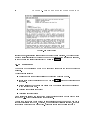
Running SNNS
After installation, the executable for the graphical user interface can be found as program
xgui in the <SNNSDIR>/xgui/sources directory. We usually build a symbolic link named
snns to point to the executable xgui program, if we often work on the same machine
architecture. E.g.:
ln -s xgui/bin/<architecture>/xgui snns
This link should be placed in the user's home directory (with the proper path prex to
SNNS) or in a directory of binaries in the local user's search path.
The simulator is then called simply with
snns
For further details about calling the various simulator tools see chapter 13.
2.4 Contact Points
If you would like to contact the SNNS team please write to Andreas Zell at
Prof. Dr. Andreas Zell
Eberhard-Karls-Universitat Tubingen
Kostlinstr. 6
72074 Tubingen
Germany
e-mail: [email protected]
12
CHAPTER 2. LICENSING, INSTALLATION AND ACKNOWLEDGMENTS
If you would like to contact other SNNS users to exchange ideas, ask for help, or distribute
advice, then post to the SNNS mailing list. Note, that you must be subscribed to it before
being able to post.
To subscribe, send a mail to
[email protected]
With the one line message (in the mail body, not in the subject)
subscribe
You will then receive a welcome message giving you all the details about how to post.
2.5 Acknowledgments
SNNS is a joint eort of a number of people, computer science students, research assistants
as well as faculty members at the Institute for Parallel and Distributed High Performance
Systems (IPVR) at University of Stuttgart, the Wilhelm Schickard Institute of Computer
Science at the University of Tubingen, and the European Particle Research Lab CERN in
Geneva.
The project to develop an eÆcient and portable neural network simulator which later
became SNNS was lead since 1989 by Prof. Dr. Andreas Zell, who designed the predecessor
to the SNNS simulator and the SNNS simulator itself and acted as advisor for more than
two dozen independent research and Master's thesis projects that made up the SNNS
simulator and some of its applications. Over time the SNNS source grew to a total
size of now 5MB in 160.000+ lines of code. Research began under the supervision of
Prof. Dr. Andreas Reuter and Prof. Dr. Paul Levi. We are all grateful for their support
and for providing us with the necessary computer and network equipment. We also would
like to thank Prof. Sau Lan Wu, head of the University of Wisconsin research group on
high energy physics at CERN in Geneva, Switzerland for her generous support of our work
towards new SNNS releases.
The following persons were directly involved in the SNNS project. They are listed in the
order in which they joined the SNNS team.
Andreas Zell
Design of the SNNS simulator, SNNS project team leader
[ZMS90], [ZMSK91b] [ZMSK91c], [ZMSK91a]
Niels Mache
SNNS simulator kernel (really the heart of SNNS) [Mac90],
parallel SNNS kernel on MasPar MP-1216.
Tilman Sommer
original version of the graphical user interface XGUI with integrated network editor [Som89], PostScript printing.
Ralf Hubner
SNNS simulator 3D graphical user interface [Hub92], user interface development (version 2.0 to 3.0).
Thomas Korb
SNNS network compiler and network description language Nessus [Kor89]
2.5. ACKNOWLEDGMENTS
Michael Vogt
Gunter Mamier
Michael Schmalzl
Kai-Uwe Herrmann
Artemis Hatzigeorgiou
Dietmar Posselt
Sven Doring
Tobias Soyez
Tobias Schreiner
Bernward Kett
Gianfranco Clemente
Henri Bauknecht
Jens Wieland
Jurgen Gatter
13
Radial Basis Functions [Vog92]. Together with Gunter Mamier
implementation of Time Delay Networks. Denition of the new
pattern format and class scheme.
SNNS visualization and analyzing tools [Mam92]. Implementation of the batch execution capability. Together with Michael
Vogt implementation of the new pattern handling. Compilation and continuous update of the user manual. Bugxes and
installation of external contributions. Implementation of pattern remapping mechanism.
SNNS network creation tool Bignet, implementation of Cascade Correlation, and printed character recognition with SNNS
[Sch91a]
ART models ART1, ART2, ARTMAP and modication of the
BigNet tool [Her92].
Video documentation about the SNNS project, learning procedure Backpercolation 1.1
ANSI-C translation of SNNS.
ANSI-C translation of SNNS and source code maintenance.
Implementation of distributed kernel for workstation clusters.
Jordan and Elman networks, implementation of the network
analyzer [Soy93].
Network pruning algorithms [Sch94]
Redesign of C-code generator snns2c.
Help with the user manual
Manager of the SNNS mailing list.
Design and implementation of batchman.
Implementation of TACOMA and some modications of Cascade Correlation [Gat96].
We are proud of the fact that SNNS is experiencing growing support from people outside
our development team. There are many people who helped us by pointing out bugs or
oering bug xes, both to us and other users. Unfortunately they are to numerous to list
here, so we restrict ourselves to those who have made a major contribution to the source
code.
1
Backpercolation 1 was developed by JURIK RESEARCH & CONSULTING, PO 2379, Aptos, CA
95001 USA. Any and all SALES of products (commercial, industrial, or otherwise) that utilize the
Backpercolation 1 process or its derivatives require a license from JURIK RESEARCH & CONSULTING. Write for details.
14
CHAPTER 2. LICENSING, INSTALLATION AND ACKNOWLEDGMENTS
Martin Riedmiller, University of Karlsruhe
Implementation of RPROP in SNNS
Martin Reczko, German Cancer Research Center (DKFZ)
Implementation of Backpropagation Through Time (BPTT),
BatchBackpropagation Through Time (BBPTT), and Quickprop Through Time (QPTT).
Mark Seemann and Marcus Ritt, University of Tubingen
Implementation of self organizing maps.
Jamie DeCoster, Purdue University
Implementation of auto-associative memory functions.
Jochen Biedermann, University of Gottingen
Help with the implementation of pruning Algorithms and noncontributing units
Christian Wehrfritz, University of Erlangen
Original implementation of the projection tool, implementation
of the statistics computation and learning algorithm Pruned
Cascade Correlation.
Randolf Werner, University of Koblenz
Support for NeXT systems
Joachim Danz, University of Darmstadt
Implementation of cross validation, simulated annealing and
Monte Carlo learning algorithms.
Michael Berthold, University of Karlsruhe
Implementation of enhanced RBF algorithms.
Bruno Orsier, University of Geneva
Implementation of Scaled Conjugate Gradient learning.
Till Brychcy, Technical University of Munich
Suplied the code to keep only the important parameters in the
control panel visible.
Joydeep Ghosh, University of Texas, Austin
Implenetation of WinSNNS, a MS-Windows front-end to SNNS
batch execution on unix workstations.
Thomas Ragg, University of Karlsruhe
Implementation of Genetic algorithm tool Enzo.
Thomas Rausch, University of Dresden
Activation function handling in batchman.
The SNNS simulator is a successor to an earlier neural network simulator called NetSim
[ZKSB89], [KZ89] by A. Zell, T. Sommer, T. Korb and A. Bayer, which was itself inuenced
by the popular Rochester Connectionist Simulator RCS [GLML89].
2.6. NEW FEATURES OF RELEASE 4.2
15
In September 1991 the Stuttgart Neural Network Simulator SNNS was awarded the
\Deutscher Hochschul-Software-Preis 1991" (German Federal Research Software Prize)
by the German Federal Minister for Science and Education, Prof. Dr. Ortleb.
2.6 New Features of Release 4.2
Users already familiar with SNNS and its usage may be interested in the dierences between the versions 4.1 and 4.2. New users of SNNS may skip this section and proceed
with the next chapter.
New Features of Release 4.2:
1. greatly improved installation procedure
2. pattern remapping functions introduced to SNNS
3. class information in patterns introduced to SNNS
4. change to all batch algorithms: The learning rate is now divided by the number of
patterns in the set. This allows for direct comparisons of learning rates and training
of large pattern les with BP-Batch since it doesn't require ridiculous learning rates
like 0.0000001 anymore.
5. Changes to Cascade-Correlation:
(a) Several modications can be used to achieve a net with a smaller depth or
smaller Fan-In.
(b) New activation functions ACT GAUSS and ACT SIN
(c) The backpropagation algorithm of Cascade-Correlation is now present in an
oline and a batch version.
(d) The activations of the units could be cached. The result is a faster learning for
nets with many units. On the other hand, the needed memory space will rise
for large training patterns.
(e) Changes in the 2D-display, the hidden units are displayed in layers, the candidate units are placed on the top of the net.
(f) validation now possible
(g) automatic deletion of candidate units at the end of training.
6. new meta learning algorithm TACOMA.
7. new learning algorithm BackpropChunk. It allows chunkwise updating of the weights
as well as selective training of units on the basis of pattern class names.
8. new learning algorithm RPROP with weight decay.
9. algorithm \Recurrent Cascade Correlation" deleted from repository.
16
CHAPTER 2. LICENSING, INSTALLATION AND ACKNOWLEDGMENTS
10. the options of adding noise to the weights with the JogWeights function improved
im multiple ways.
11. improved plotting in the graph panel as well as printing option
12. when standard colormap is full, SNNS will now start with a privat map instead of
aborting.
13. analyze tool now features a confusion matrix.
14. pruning panel now more \SNNS-like". You do not need to close the panel anymore
before pruning a network.
15. Changes in batchman
(a) batchman can now handle DLVQ training
(b) new batchman command \setActFunc" allows the changing of unit activation
functions from within the training script. Thanks to Thomas Rausch, University of Dresden, Germany.
(c) batchman output now with \#" prex. This enables direct processing by a lot
of unix tools like gnuplot.
(d) batchman now automatically converts function parameters to correct type instead of aborting.
(e) jogWeights can now also be called from batchman
(f) batchman catches some non-fatal signals (SIGINT, SIGTERM, ...) and sets
the internal variable SIGNAL so that the script can react to them.
(g) batchman features ResetNet function (e.g. for Jordan networks).
16. new tool \linknets" introduced to combine existing networks
17. new tools \td bignet" and \ bignet" introduced for script-based generation of network les; Old tool bignet removed.
18. displays will be refreshed more often when using the graphical editor
19. weight and projection display with changed color scale. They now match the 2Ddisplay scale.
20. pat sel now can handle pattern les with multi-line comments
21. manpages now available for most of the SNNS programs.
22. the number of things stored in an xgui conguration le was greatly enhanced.
23. Extensive debugging:
(a) batchman computes MSE now correctly from the number of (sub-) patterns.
(b) RBFs receive now correct number of parameters.
(c) spurious segmentation faults in the graphical editor tracked and eliminated.
(d) segmentation fault when training on huge pattern les cleared.
2.6. NEW FEATURES OF RELEASE 4.2
17
(e) various seg-faults under single operating systems tracked and cleared.
(f) netperf now can test on networks that need multiple training parameters.
(g) segmentaion faults when displaying 3D-Networks cleared.
(h) correct default values for initialization functions in batchman.
(i) the call \TestNet()" prohibited further training in batchman. Now everything
works as expected.
(j) segmentation fault in batchman when doing multiple string concats cleared and
memory leak in string operations closed. Thanks to Walter Prins, University
of Stellenbosch, South Africa.
(k) the output of the validation error on the shell window was giving wrong values.
(l) algorithm SCG now respects special units and handles them correctly.
(m) the description of the learning function parameters in section 4.4 is nally
ordered alphabetically.
Chapter 3
Neural Network Terminology
is a current focus of research in a number of disciplines, among them
articial intelligence (or more general computer science), physics, psychology, linguistics,
biology and medicine. Connectionism represents a special kind of information processing:
Connectionist systems consist of many primitive cells (units ) which are working in parallel
and are connected via directed links (links, connections ). The main processing principle
of these cells is the distribution of activation patterns across the links similar to the basic
mechanism of the human brain, where information processing is based on the transfer of
activation from one group of neurons to others through synapses. This kind of processing
is also known as parallel distributed processing (PDP).
The high performance of the human brain in highly complex cognitive tasks like visual
and auditory pattern recognition was always a great motivation for modeling the brain.
For this historic motivation connectionist models are also called neural nets . However,
most current neural network architectures do not try to closely imitate their biological
model but rather can be regarded simply as a class of parallel algorithms.
In these models, knowledge is usually distributed throughout the net and is stored in
the structure of the topology and the weights of the links. The networks are organized
by (automated) training methods, which greatly simplify the development of specic applications. Classical logic in ordinary AI systems is replaced by vague conclusions and
associative recall (exact match vs. best match). This is a big advantage in all situations
where no clear set of logical rules can be given. The inherent fault tolerance of connectionist models is another advantage. Furthermore, neural nets can be made tolerant against
noise in the input: with increased noise, the quality of the output usually degrades only
slowly (graceful performance degradation ).
Connectionism
3.1 Building Blocks of Neural Nets
The following paragraph describes a generic model for those neural nets that can be
generated by the SNNS simulator. The basic principles and the terminology used in
dealing with the graphical interface are also briey introduced. A more general and more
detailed introduction to connectionism can, e.g., be found in [RM86]. For readers uent
19
3.1. BUILDING BLOCKS OF NEURAL NETS
in German, the most comprehensive and up to date book on neural network learning
algorithms, simulation systems and neural hardware is probably [Zel94]
A network consists of units 1 and directed, weighted links (connections) between them. In
analogy to activation passing in biological neurons, each unit receives a net input that is
computed from the weighted outputs of prior units with connections leading to this unit.
Picture 3.1 shows a small network.
output unit
11.71
-5.24
-5.24
6.97
hidden unit
6.97
input units
Figure 3.1: A small network with three layers of units
The actual information processing within the units is modeled in the SNNS simulator with
the activation function and the output function. The activation function rst computes
the net input of the unit from the weighted output values of prior units. It then computes
the new activation from this net input (and possibly its previous activation). The output
function takes this result to generate the output of the unit.2 These functions can be
arbitrary C functions linked to the simulator kernel and may be dierent for each unit.
Our simulator uses a discrete clock. Time is not modeled explicitly (i.e. there is no
propagation delay or explicit modeling of activation functions varying over time). Rather,
the net executes in update steps , where a(t + 1) is the activation of a unit one step after
a(t).
The SNNS simulator, just like the Rochester Connectionist Simulator (RCS, [God87]),
oers the use of sites as additional network element. Sites are a simple model of the
dendrites of a neuron which allow a grouping and dierent treatment of the input signals
of a cell. Each site can have a dierent site function. This selective treatment of incoming
information allows more powerful connectionist models. Figure 3.2 shows one unit with
sites and one without.
In the following all the various network elements are described in detail.
3.1.1 Units
Depending on their function in the net, one can distinguish three types of units: The
units whose activations are the problem input for the net are called input units ; the units
In the following the more common name "units" is used instead of "cells".
The term transfer function often denotes the combination of activation and output function. To make
matters worse, sometimes the term activation function is also used to comprise activation and output
function.
1
2
20
CHAPTER 3. NEURAL NETWORK TERMINOLOGY
unit with sites
unit without sites
to other units
to other units
output
output function
output
output function
activation
activation function
activation
activation function
site value
site function
Figure 3.2: One unit with sites and one without
whose output represent the output of the net output units. The remaining units are called
because they are not visible from the outside (see e.g. gure 3.1).
In most neural network models the type correlates with the topological position of the
unit in the net: If a unit does not have input connections but only output connections,
then it is an input unit. If it lacks output connections but has input units, it is an output
unit. If it has both types of connections it is a hidden unit.
It can, however, be the case that the output of a topologically internal unit is regarded
as part of the output of the network. The IO-type of a unit used in the SNNS simulator
has to be understood in this manner. That is, units can receive input or generate output
even if they are not at the fringe of the network.
Below, all attributes of a unit are listed:
no: For proper identication, every unit has a number3 attached to it. This number
denes the order in which the units are stored in the simulator kernel.
name: The name can be selected arbitrarily by the user. It must not, however,
contain blanks or special characters, and has to start with a letter. It is useful
to select a short name that describes the task of the unit, since the name can be
displayed with the network.
io-type or io: The IO-type denes the function of the unit within the net. The
following alternatives are possible
{ input : input unit
{ output : output unit
{ dual : both input and output unit
hidden units ,
3
This number can change after saving but remains unambiguous. See also chapter 4.3.2.1
3.1. BUILDING BLOCKS OF NEURAL NETS
21
{ hidden : internal, i.e. hidden unit
{ special: this type can be used in any way, depending upon the application.
In
the standard version of the SNNS simulator, the weights to such units are not
adapted in the learning algorithm (see paragraph 3.3).
{ special input, special hidden, special output : sometimes it is necessary to to
know where in the network a special unit is located. These three types enable
the correlation of the units to the various layers of the network.
activation: The activation value.
initial activation or i act: This variable contains the initial activation value,
present after the initial loading of the net. This initial conguration can be reproduced by resetting (reset ) the net, e.g. to get a dened starting state of the net.
output: the output value.
bias: In contrast to other network simulators where the bias (threshold) of a unit
is simulated by a link weight from a special 'on'-unit, SNNS represents it as a unit
parameter. In the standard version of SNNS the bias determines where the activation
function has its steepest ascent. (see e.g. the activation function Act logistic).
Learning procedures like backpropagation change the bias of a unit like a weight
during training.
activation function or actFunc: A new activation is computed from the output
of preceding units, usually multiplied by the weights connecting these predecessor
units with the current unit, the old activation of the unit and its bias. When sites
are being used, the network input is computed from the site values. The general
formula is:
aj (t + 1) = fact (netj (t); aj (t); j )
where:
aj (t)
activation of unit j in step t
netj (t) net input in unit j in step t
j
threshold (bias) of unit j
The SNNS default activation function Act logistic , for example, computes the network input simply by summing over all weighted activations and then squashing the
result with the logistic function fact(x) = 1=(1 + e x). The new activation at time
(t + 1) lies in the range [0; 1]4 . The variable j is the threshold of unit j .
The net input netj (t) is computed with
netj (t) =
wij oi (t) if unit j has no sites
X
netj (t)
4
=
i
X
k
sjk (t)
if the unit j has sites, with site values
Mathematically correct would be ]0; 1[, but the values 0 and 1 are reached due to arithmetic inaccuracy.
22
CHAPTER 3. NEURAL NETWORK TERMINOLOGY
sjk (t)
=
X
i
wij oi (t)
This yields the well-known logistic activation function
1
aj (t + 1) =
1 + e ( w o (t) )
P
i
ij i
j
where:
aj (t)
netj (t)
oi (t)
sjk (t)
activation of unit j in step t
net input in unit j in step t
output of unit i in step t
site value of site k on unit j in step t
j
index for some unit in the net
i
index of a predecessor of the unit j
k
index of a site of unit j
wij
weight of the link from unit i to unit j
j
threshold (bias) of unit j
Activation functions in SNNS are relatively simple C functions which are linked to
the simulator kernel. The user may easily write his own activation functions in C and
compile and link them to the simulator kernel. How this can be done is described
later.
output function or outFunc: The output function computes the output of every
unit from the current activation of this unit. The output function is in most cases
the identity function (SNNS: Out identity). This is the default in SNNS. The
output function makes it possible to process the activation before an output occurs.
oj (t) = fout (aj (t))
where:
aj (t) Activation of unit j in step t
oj (t) Output of unit j in step t
j
Index for all units of the net
Another predened SNNS-standard function,
range of [0::1] and is dened as follows:
8
>
<
oj (t) = >
:
Out Clip01
clips the output to the
0
1
if aj (t) < 0
if aj (t) > 1
aj (t) otherwise
Output functions are even simpler C functions than activation functions and can be
user-dened in a similar way.
3.1. BUILDING BLOCKS OF NEURAL NETS
23
The user can assign so called f-types (functionality types, prototypes) to
a unit. The unusual name is for historical reasons. One may think of an f-type as
a pointer to some prototype unit where a number of parameters has already been
dened:
{ activation function and output function
{ whether sites are present and, if so, which ones
These types can be dened independently and are used for grouping units into sets
of units with the same functionality. All changes in the denition of the f-type
consequently aect also all units of that type. Therefore a variety of changes becomes
possible with minimum eort.
position: Every unit has a specic position (coordinates in space) assigned to it.
These positions consist of 3 integer coordinates in a 3D grid. For editing and 2D
visualization only the rst two (x and y) coordinates are needed, for 3D visualization
of the networks the z coordinate is necessary.
subnet no: Every unit is assigned to a subnet. With the use of this variable,
structured nets can be displayed more clearly than would otherwise be possible in a
2D presentation.
layers: Units can be visualized in 2D in up to 8 layers5 . Layers can be displayed
selectively. This technique is similar to a presentation with several transparencies,
where each transparency contains one aspect or part of the picture, and some or all
transparencies can be selected to be stacked on top of each other in a random order.
Only those units which are in layers (transparencies) that are 'on' are displayed.
This way portions of the network can be selected to be displayed alone. It is also
possible to assign one unit to multiple layers. Thereby it is feasible to assign any
combination of units to a layer that represents an aspect of the network.
frozen: This attribute ag species that activation and output are frozen. This
means that these values don't change during the simulation.
All `important' unit parameters like activation, initial activation, output etc. and all function results are computed as oats with nine decimals accuracy.
f-type:
3.1.2 Connections (Links)
The direction of a connection shows the direction of the transfer of activation. The unit
from which the connection starts is called the source unit , or source for short, while the
other is called the target unit , or target. Connections where source and target are identical
(recursive connections) are possible. Multiple connections between one unit and the same
input port of another unit are redundant, and therefore prohibited. This is checked by
SNNS.
Each connection has a weight (or strength) assigned to it. The eect of the output of one
unit on the successor unit is dened by this value: if it is negative, then the connection
5
Changing it to 16 layers can be done very easily in the source code of the interface.
24
CHAPTER 3. NEURAL NETWORK TERMINOLOGY
is inhibitory, i.e. decreasing the activity of the target unit; if it is positive, it has an
excitatory, i.e. activity enhancing, eect.
The most frequently used network architecture is built hierarchically bottom-up. The input into a unit comes only from the units of preceding layers. Because of the unidirectional
ow of information within the net they are also called feed-forward nets (as example see
the neural net classier introduced in chapter 3.5). In many models a full connectivity
between all units of adjoining levels is assumed.
Weights are represented as oats with nine decimal digits of precision.
3.1.3 Sites
A unit with sites doesn't have a direct input any more. All incoming links lead to dierent
sites, where the arriving weighted output signals of preceding units are processed with
dierent user-denable site functions (see picture 3.2). The result of the site function is
represented by the site value. The activation function then takes this value of each site as
network input.
The SNNS simulator does not allow multiple connections from a unit to the same input
port of a target unit. Connections to dierent sites of the same target units are allowed.
Similarly, multiple connections from one unit to dierent input sites of itself are allowed
as well.
3.2 Update Modes
To compute the new activation values of the units, the SNNS simulator running on a
sequential workstation processor has to visit all of them in some sequential order. This
order is dened by the Update Mode . Five update modes for general use are implemented
in SNNS. The rst is a synchronous mode, all other are asynchronous, i.e. in these modes
units see the new outputs of their predecessors if these have red before them.
1. synchronous : The units change their activation all together after each step. To do
this, the kernel rst computes the new activations of all units from their activation
functions in some arbitrary order. After all units have their new activation value
assigned, the new output of the units is computed. The outside spectator gets the
impression that all units have red simultaneously (in sync).
2. random permutation : The units compute their new activation and output function
sequentially. The order is dened randomly, but each unit is selected exactly once
in every step.
3. random : The order is dened by a random number generator. Thus it is not guaranteed that all units are visited exactly once in one update step, i.e. some units may
be updated several times, some not at all.
4. serial : The order is dened by ascending internal unit number. If units are created
with ascending unit numbers from input to output units, this is the fastest mode.
3.3. LEARNING IN NEURAL NETS
25
Note that the use of serial mode is not advisable if the units of a network are not in
ascending order.
5. topological : The kernel sorts the units by their topology. This order corresponds to
the natural propagation of activity from input to output. In pure feed-forward nets
the input activation reaches the output especially fast with this mode, because many
units already have their nal output which doesn't change later.
Additionally, there are 12 more update modes for special network topologies implemented
in SNNS.
1. CPN : For learning with counterpropagation.
2. Time Delay : This mode takes into account the special connections of time delay
networks. Connections have to be updated in the order in which they become valid
in the course of time.
3. ART1 Stable, ART2 Stable and ARTMAP Stable : Three update modes for the three
adaptive resonance theory network models. They propagate a pattern through the
network until a stable state has been reached.
4. ART1 Synchronous, ART2 Synchronous and ARTMAP Synchronous : Three other
update modes for the three adaptive resonance theory network models. They perform
just one propagation step with each call.
5. CC : Special update mode for the cascade correlation meta algorithm.
6. BPTT : For recurrent networks, trained with `backpropagation through time'.
7. RM Synchronous : Special update mode for auto-associative memory networks.
Note, that all update modes only apply to the forward propagation phase, the backward
phase in learning procedures like backpropagation is not aected at all.
3.3 Learning in Neural Nets
An important focus of neural network research is the question of how to adjust the weights
of the links to get the desired system behavior. This modication is very often based on
the Hebbian rule, which states that a link between two units is strengthened if both units
are active at the same time. The Hebbian rule in its general form is:
wij = g(aj (t); tj )h(oi (t); wij )
where:
wij
aj (t)
tj
oi (t)
weight of the link from unit i to unit j
activation of unit j in step t
teaching input, in general the desired output of unit j
output of unit i at time t
26
CHAPTER 3. NEURAL NETWORK TERMINOLOGY
g(: : :)
h(: : :)
function, depending on the activation of the unit and the teaching input
function, depending on the output of the preceding element and the current
weight of the link
Training a feed-forward neural network with supervised learning consists of the following
procedure:
An input pattern is presented to the network. The input is then propagated forward in
the net until activation reaches the output layer. This constitutes the so called forward
propagation phase.
The output of the output layer is then compared with the teaching input. The error,
i.e. the dierence (delta) Æj between the output oj and the teaching input tj of a target
output unit j is then used together with the output oi of the source unit i to compute
the necessary changes of the link wij . To compute the deltas of inner units for which no
teaching input is available, (units of hidden layers) the deltas of the following layer, which
are already computed, are used in a formula given below. In this way the errors (deltas)
are propagated backward, so this phase is called backward propagation.
In online learning, the weight changes wij are applied to the network after each training
pattern, i.e. after each forward and backward pass. In oine learning or batch learning
the weight changes are cumulated for all patterns in the training le and the sum of all
changes is applied after one full cycle (epoch) through the training pattern le.
The most famous learning algorithm which works in the manner described is currently
backpropagation. In the backpropagation learning algorithm online training is usually
signicantly faster than batch training, especially in the case of large training sets with
many similar training examples.
The backpropagation weight update rule, also called generalized delta-rule reads as follows:
wij =
Æj =
Æj oi
(
fj0 (netj )(P
tj oj )
0
fj (netj ) k Æk wjk
if unit j is a output-unit
if unit j is a hidden-unit
where:
learning factor eta (a constant)
Æj error (dierence between the real output and the teaching input) of unit j
tj teaching input of unit j
oi output of the preceding unit i
i index of a predecessor to the current unit j with link wij from i to j
j index of the current unit
k index of a successor to the current unit j with link wjk from j to k
There are several backpropagation algorithms supplied with SNNS: one \vanilla backpropagation" called Std Backpropagation, one with momentum term and at spot elimination
called BackpropMomentum and a batch version called BackpropBatch. They can be chosen from the control panel with the button OPTIONS and the menu selection select
learning function.
3.4. GENERALIZATION OF NEURAL NETWORKS
27
In SNNS, one may either set the number of training cycles in advance or train the network
until it has reached a predened error on the training set.
3.4 Generalization of Neural Networks
Figure 3.3: Error development of a training and a validation set
One of the major advantages of neural nets is their ability to generalize. This means that
a trained net could classify data from the same class as the learning data that it has never
seen before. In real world applications developers normally have only a small part of all
possible patterns for the generation of a neural net. To reach the best generalization, the
dataset should be split into three parts:
The training set is used to train a neural net. The error of this dataset is minimized
during training.
The validation set is used to determine the performance of a neural network on
patterns that are not trained during learning.
A test set for nally checking the over all performance of a neural net.
Figure 3.3 shows a typical error development of a training set (lower curve) and a validation
set (upper curve).
The learning should be stopped in the minimum of the validation set error. At this
point the net generalizes best. When learning is not stopped, overtraining occurs and the
performance of the net on the whole data decreases, despite the fact that the error on
the training data still gets smaller. After nishing the learning phase, the net should be
nally checked with the third data set, the test set.
SNNS performs one validation cycle every n training cycles. Just like training, validation
is controlled from the control panel.
28
CHAPTER 3. NEURAL NETWORK TERMINOLOGY
3.5 An Example of a simple Network
Figure 3.4: Example network of the letter classier
This paragraph describes a simple example network, a neural network classier for capital
letters in a 5x7 matrix, which is ready for use with the SNNS simulator. Note that this is
a toy example which is not suitable for real character recognition.
Network-Files: letters untrained.net, letters.net (trained)
Pattern-File: letters.pat
The network in gure 3.4 is a feed-forward net with three layers of units (two layers of
weights) which can recognize capital letters. The input is a 5x7 matrix, where one unit
is assigned to each pixel of the matrix. An activation of +1:0 corresponds to \pixel set",
while an activation value of 0:0 corresponds to \pixel not set". The output of the network
consists of exactly one unit for each capital letter of the alphabet.
The following activation function and output function are used by default:
Activation function: Act logistic
Output function: Out identity
The net has one input layer (5x7 units), one hidden layer (10 units) and one output layer
(26 units named 'A' . ..'Z'). The total of (35 10 + 10 26) = 610 connections form the
distributed memory of the classier.
On presentation of a pattern that resembles the uppercase letter \A", the net produces
as output a rating of which letters are probable.
Chapter 4
Using the Graphical User Interface
This chapter describes how to use XGUI, the X-Window based graphical user interface to
SNNS, which is the usual way to interact with SNNS on Unix workstations. It explains
how to call SNNS and details the multiple windows and their buttons and menus. Together
with the chapters 5 and 6 it is probably the most important chapter in this manual.
4.1 Basic SNNS usage
SNNS is a very comprehensive package for the simulation of neural networks. It may look
a little daunting for rst time users. This section is intended as a quick starter for using
SNNS. Refer to the other chapters of this manual for more detailed information.
Before using SNNS your environment should be changed to include the relevant directories.
This is done by :
1. copy the le SNNSv4.2/default.cfg to your favorite directory
2. copy the le SNNSv4.2/help.hdoc to your favorite directory
3. Set the environment variable XGUILOADPATH to this directory with the command setenv XGUILOADPATH your directory path. You could add this line to
your .login le, so that the help and conguration les are available whenever
SNNS is started.
4.1.1 Startup
SNNS comes in two guises: It can be used via an X-windows user interface, or in 'batch
mode', that is without user interaction. To run it with the X-GUI, type snns. You
obviously need an X-terminal. The default setting for SNNS is to use colour screens,
if you use a monochrome X-terminal start it up using snns -mono. You will loose no
functionality - some things are actually clearer in black and white.
30
CHAPTER 4. USING THE GRAPHICAL USER INTERFACE
After starting the package a banner will appear which will vanish after you click the left
mouse button in the panel. You are then left with the SNNS manager panel.
File
handling
Training &
testing control
Information
about single units
or weights
Network
Diagram
Error Graph
Network
Definition
Exit
Help
Figure 4.1: The SNNS manager panel
The SNNS manager allows you to access all functions oered by the package. It is a
professional tool and you may nd it a little intimidating. You will not need to use the
majority of the options. You should read this introduction while running the simulator the whole thing is quite intuitive and you will nd your way around it very quickly.
4.1.2 Reading and Writing Files
SNNS supports ve types of les, the most important ones are:
NET Network denition les containing information on network topology and learning
rules. The les end in the extension '.net'.
PAT Pattern les, containing the training and test data. All pattern les end in '.pat'.
RES Results les. Network output is interpreted in many possible ways, depending on
the problem. SNNS allows the user to dump the network outputs into a separate
le for later analysis.
The other two le types are not important for a rst exploration of SNNS.
The rst thing you are likely to use is the FILE option in the manager panel to read
network and pattern denition les. The window that will appear is given in gure 4.2.
The top text eld shows the current directory. The main eld shows all les for each of
the le types that SNNS can read/write. Directories are marked by square brackets. To
load an example network change the directory by entering the example directory path in
the top eld (do not press return):
SNNSv4.2/examples
Changes will only be apparent after one of the le selectors has been touched:click on
PAT and then NET again. You should now see a list of all network denition les
31
4.1. BASIC SNNS USAGE
current directory
file name
file type selectors
list of existing
files
scrollbar
click here to
load
save
click here when done
Figure 4.2: The SNNS le browser
currently available. Double-clicking on one of the lenames, say 'letters' will copy the
network name into the le name window. To load the network simply click on LOAD .
You can also enter the lename directly into the le name window (top left).
4.1.3 Creating New Networks
You will need to create your own networks. SNNS allows the creation of many dierent
network types. Here is an example of how to create a conventional (fully connected)
feed-forward network.
First select the GENERAL option, hidden under the BIGNET button in the manager
panel. You are then faced with the panel in gure 4.3. Only two parts of the panel are
required.
The top allows the denition of the network topology, that is how many units are required
in each layer and how they should appear if the network is displayed on the screen. The
lower part allows you to fully connect the layers and to create the network.
Note that much of what you are dening here is purely cosmetic. The pattern les contain
a given number of inputs and outputs, they have to match the network topology; how
they are arranged in the display is not important for the functionality.
First you have to dene the input layer by lling the blanks in the top right hand corner
(edit plane) of the panel. The panel shows the current settings for each group of units (a
plane in SNNS terminology). Each group is of a given type (i.e. input, hidden or output),
and each plane contains a number of units arranged in an x-y-z coordinate system. This
is used for drawing networks only!
You can change the entries by entering values into the boxes or by clicking on TYPE and
32
CHAPTER 4. USING THE GRAPHICAL USER INTERFACE
enter layer topology here
ENTER
defines plane
select TYPE and POS to change
unit types and relative position
at the moment
ignore all this
click here to fully connect all layers
as the last step
create network
here
Figure 4.3: The SNNS BigNet Feedforward network designer panel
POS to change the unit type and relative position. The relative position is not used for
the rst plane of units (there is nothing to position it relatively to). The layers will, for
instance, be positioned below the previous layers if the 'Rel. Position' has been changed
to 'below' by clicking on the POS button.
Here is an example of how to create a simple pattern associator network with a 5x7 matrix
of inputs inputs, 10 hidden units and 26 outputs:
Leave 'Type' as input
set no 'x' direction to 5
set no 'y' direction to 7
and click on ENTER
If the input is acceptable it will be copied to the column to the left. The next step is to
dene the hidden layer, containing 10 units, positioned to the right the inputs.
4.1. BASIC SNNS USAGE
33
Change 'Type' from input to hidden by clicking on TYPE once.
set no 'x' direction to 1
set no 'y' direction to 10
change 'Rel.Position' to 'below' by clicking on POS
and click on ENTER
You are now ready to dene the output plane, here you want 26 output units to the right
of the input. You may want to save space and arrange the 26 outputs as two columns of
13 units each.
Change 'Type' from hidden to output by clicking on TYPE again.
set no 'x' direction to 2
set no 'y' direction to 13
and click on ENTER
After dening the layer topology the connections have to be made. Simply click on
FULL CONNECTION (bottom left of lower panel). Then select CREATE NET and
DONE . You may have to conrm the destruction of any network already present.
Selection of DISPLAY from the SNNS-manager panel should result in gure 4.4.
Figure 4.4: SNNS network display panel
The lines showing the weights are not normally visible, you have to switch them on by
selecting SETUP , and then clicking on the ON button next to 'links' option. You will
nd that SNNS refuses any further input until you have selected DONE .
After creating the network and loading in the pattern le(s) - which have to t the network
topology - you can start training the net. The network you have just created should t
the \letters" patterns in the SNNS examples directory.
An alternate way to construct a network is via the graphical network editor build into
SNNS. It is best suited to alter an existing large network or to create a new small one. For
the creation of large networks use bignet. The network editor is described in chapter 6.
34
CHAPTER 4. USING THE GRAPHICAL USER INTERFACE
4.1.4 Training Networks
Load the 'letters' pattern le (in the SNNS examples directory) at this stage. The network
is a pattern associator that can be trained to map an input image (5x7 pixel representation
of letters) into output units where each letter is represented by an output unit.
All training and testing is done via the control panel. It is opened by clicking on the
CONTROL button of the manager panel. The most important features of this panel will
now be discussed one by one. The panel consists of two parts. The top part controls the
parameters dening the training process, the bottom four rows are blanks that have to be
lled in to dene the learning rates and the range over which weights will be randomly
distributed when the network is initialised, etc. The defaults for the learning parameters
are (0.2 0) while the default weight setting is between 1 and -1 (1.0 -1.0).
4.1.4.1 Initialization
Many networks have to be initialised before they can be used. To do this, click on INIT
(top line of buttons in control). You can change the range of random numbers used in the
initialization by entering appropriate values into the elds to the right of \INIT" at the
lower end of the control panel.
enter no of cycles here
start / stop training
Training
Control
Parameters
initialize network
click here to
present patterns
in random order
Select learning
function from this
button
Learning
Parameters
click here when done
Figure 4.5: SNNS network training and testing control panel
4.1.4.2 Selecting a learning function
The default learning function for feed-forward nets is Std Backpropagation, you may want
something a little more extravagant. Simply click on SEL FUNC (Select function next
to the learning parameters, see gure 4.5) and pick what you want to use. The routines
you may want to consider are Std Backpropagation, BackpropMomentum or Rprop). Use
BackpropMomentum for the letters example.
4.1. BASIC SNNS USAGE
35
Each learning function requires a dierent parameter set: here are the important ones,
details are given in the manual:
Std Backpropagation 1: learning rate (0-1), 2: dmax , the maximum error that is
tolerated. use 0 or a small value.
BackpropMomentum 1: learning rate (0-1), 2: momentum term (0-0.99), 3: c at
spot elimination (ignore) and 4: dmax max ignored error.
Rprop 1: starting values of ij (0-0.2) 2: max maximum update value (30 works well..)
3: the weight decay term as an exponent (5 works for most problems) x = 10 =
0:00001.
Once all parameters are set you are ready to do some training. Training is done for a
number of 'CYCLES' or epochs (enter a number, say 200 - see g. 4.5). All training
patterns are presented once during each cycle. It is sometimes preferable to select the
patterns randomly for presentation rather than in order: Click on SHUFFLE to do this.
For the pattern associator example leave the learning rate at 0.2 and set the momentum
term (second eld) to 0.5; leave everything else at 0.
Before starting the learning process you may like to open a GRAPH panel (from the
manager panel) to monitor the progress during training.1
Click on ALL to start training and STOP to interrupt training at any time. The graph
will start on the left whenever the network is initialised so that it is easy to compare
dierent learning parameters. The current errors are also displayed on the screen so that
they could be used in any graph plotting package (like xmgr).
It is impossible to judge the network performance from the training data alone. It is
therefore sensible to load in a 'test' set once in a while to ensure that the net is not
over-training and generalising correctly. There is no test set for the letters example. You
can have up to 5 dierent data sets active at any one time. The two USE buttons on
the control panel allow you to select which data sets to use for training and validation.
The top button selects the training set, the bottom one the 'validation set'. If you enter
a non-zero value into the box next to VALID a validation data set will be tested and
the root-mean-square error will be plotted on the graph in red every N cycles (N is the
number you entered in the box).
You can also step through all the patterns in a data set and, without updating any weight,
calculate the output activations. To step through the patterns click on TEST .
You can go to any pattern in the training data set by either specifying the pattern number
in the eld next to 'PATTERN' and clicking on GOTO or by using the 'tape player
controls' positioned to the right of GOTO . The outputs given by the network when
stepping though the data are the targets, not the calculated outputs (!).
If you do this scale the y-range to lie between 0 and 26 by clicking on the 'right-arrow' next the 'Scale
Y:' a few times. You can also resize the window containing the graph.
1
36
CHAPTER 4. USING THE GRAPHICAL USER INTERFACE
4.1.5 Saving Results for Testing
Network performance measures depend on the problem. If the network has to perform a
classication task it is common to calculate the error as a percentage of correct classications. It is possible to tolerate quite high errors in the output activations. If the network
has to match a smooth function it may be most sensible to calculate the RMS error over
all output units etc.
The most sensible way to progress is to save the output activations together with target
values for the test data and to write a little program that does whatever testing is required.
The RES les under FILE are just the ticket: Note that the output patterns are always
saved. The 'include output patterns' actually means 'include target (!) patterns'.
4.1.6 Further Explorations
It is possible to visualize the weights by plotting them, just like the output values as boxes
of dierent sizes/colour. Sometimes examining the weights gives helpful insights into how
the networks work. Select WEIGHTS from the manager panel to see the weight diagram.
4.1.7 SNNS File Formats
4.1.7.1 Pattern les
To train a network on your own data you rst have to massage the data into a format
that SNNS can understand. Fortunately this is quite easy. SNNS data les have a header
component and a data component. The header denes how many patterns the le contains
as well as the dimensionality of the input and target vectors. The les are saved as ASCII
test. An example is given in gure 4.6.
The header has to conform exactly to the SNNS format, so watch out for extra spaces etc.
You may copy the header from one of the example pattern les and to edit the numbers,
or use the tool mkhead from the tools directory. The data component of the pattern le is
simply a listing of numbers that represent the activations of the input and output units.
For each pattern the number of values has to match the number of input plus the number
of output units of the network as dened in the header. For clarity you may wish to
put comments (lines starting with a hash (#)) between your patterns like shown in gure
4.6. They are ignored by SNNS but may be used by some pattern processing tools. The
pattern denitions may have 'CR' characters (Carriage Return) in them.
Note that while the results saved by SNNS use (almost) the same le format as used for
the pattern les, the label values dened in the pattern les are not used.
4.1.7.2 Network les
The networks les, just as the pattern and result les are stored as ASCII les, they are
relatively easy to read and you may nd it easier to hand-edit the network denition le
37
4.2. XGUI FILES
SNNS pattern definition file V3.2
generated at Wed Aug 9 11:01:29 1995
File header
No. of patterns : 4772
No. of input units : 16
No. of output units : 1
# 2
0 2
# 4
1 2
# 10
0 2
# 12
0 0
# 14
0 2
2 0 -1 -1 0.91 0.91 0 1 0 0 0.01 0.01 0.34 -0.09 0.0 data
2 1 -1 4 2.93 2.93 0 0.95 0 0 0 0 0 0.75 1.0
every new pattern
starts with #label
2 0 1 2 3.43 2.15 0 0.94 0 0 0 0 0 0.65 1.0
2 0 1 -1 2.89 2.89 0 0.95 0 0 0 0 0 0.78 0.0
0 0 -1 -1 2.59 ...
could also use
# input
0 1 0 0 1
# target
1
etc
Figure 4.6: Pattern le diagram
than to use the graphical user interface to perform tasks such as changing the unit transfer
function or to change the network topology.
4.2 XGUI Files
The graphical user interface consists of the following les:
xgui
SNNS simulator program (XGUI and simulator kernel
linked together into one executable program)
default.cfg default conguration (see chapter 4.3.2)
help.hdoc
help text used by XGUI
The le Readme xgui contains changes performed after printing of this document. The user
is urged to read it, prior to using XGUI. The le help.hdoc is explained in chapter 4.3.11.
XGUI looks for the les default.cfg and help.hdoc rst in the current directory. If not
found there, it looks in the directory specied by the environment variable XGUILOADPATH.
By the command
setenv XGUILOADPATH Path
this variable can be set to the path where default.cfg and help.hdoc are located. This
is best done by an entry to the les .login or .cshrc. Advanced users may change the
help le or the default conguration for their own purposes. This should be done, however,
only on a copy of the les in a private directory.
SNNS uses the following extensions for its les:
38
CHAPTER 4. USING THE GRAPHICAL USER INTERFACE
.net
.pat
.cfg
.txt
.res
network les (units and link weights)
pattern les
conguration settings les
text les (log les)
result les (unit activations)
A simulator run is started by the command
xgui [<netfile>.net] [<pattern>.pat] [<config>.cfg] [options] Return
where valid options are
-font <name> : font for the simulator
-dfont <name> : font for the displays
-mono : black & white on color screens
-help : help screen to explain the options
in the installation directory of SNNS or by directly calling
<SNNS-directory>/xgui/bin/<architecture>/xgui
from any directory. Note that the shell variable XGUILOADPATH must be set properly
before, or SNNS will complain about missing les default.cfg and help.hdoc.
The executable xgui may also be called with X-Window parameters as arguments.
Setting the display font can be advisable, if the font selected by the SNNS automatic font
detection looks ugly. The following example starts the display with the 7x13bold font
snns -font 7x13bold Return
The fonts which are available can be detected with the program xfontsel (not part of this
distribution).
4.3 Windows of XGUI
The graphical user interface has the following windows, which can be positioned and
handled independently (toplevel shells ):
Manager panel with buttons to open other windows, a message line, and a line with
status information at the bottom .
File browser for loading and saving networks and pattern les.
Control panel for simulator operations.
Info panel for setting and getting information about unit and link attributes.
several Displays, to display the network graphically in two dimensions.
3D View panel to control the three dimensional network visualization component.
4.3. WINDOWS OF XGUI
39
Graph display, to explain the network error during teaching graphically.
Class panel to control the composition of the training pattern le.
Bignet panel to facilitate the creation of big regular networks.
Pruning panel for control of the pruning algorithm.
Cascade panel for control of the learning phase of cascade correlation and TACOMA
Kohonen panel, an extension to the control panel for Kohonen networks.
Weight Display, to show the weight matrix as a WV- or Hinton diagram.
Projection panel to clarify the inuence of two units onto a third one.
Analyzer for supervising recurrent (and other) networks.
Inversion display, to control the inversion method network analysing tool.
Print panel to generate a Postscript picture of one of the 2D displays.
Help windows to display the help text.
learning.
Of these windows only the Manager panel and possibly one or more 2D displays are
open from the start, the other windows are opened with the corresponding buttons in the
manager panel or by giving the corresponding key code while the mouse pointer is in one
of the SNNS windows.
Additionally, there are several popup windows (transient shells ) which only become visible
when called and block all other XGUI windows. Among them are various Setup panels
for adjustments of the graphical representation. (called with the button SETUP in the
various windows)
There are a number of other popup windows which are invoked by pressing a button in
one of the main windows or choosing a menu.
Figure 4.7 shows a typical screen setup. The Manager panel contains buttons to call all
other windows of the interface and displays the status of SNNS. It should therefore always
be kept visible.
The Info panel displays the attributes of two units and the data of the link between them.
All attributes may also be changed here. The data displayed here is important for many
editor commands.
In each of the Displays a part of the network is displayed, while all settings can be
changed using Setup. These windows also allow access to the network editor using the
keyboard (see also chapter 6).
The Control panel controls the simulator operations during learning and recall.
In the File panel a log le can be specied, where all XGUI output to stdout is copied
to. A variety of data about the network can be displayed here. Also a record is kept on
the load and save of les and on the teaching.
40
CHAPTER 4. USING THE GRAPHICAL USER INTERFACE
Figure 4.7: Manager panel, info panel, control panel and a display.
The complete help text from the le help.hdoc is available in the text section of a help
window. Information about a word can be retrieved by marking that word in the text and
then clicking LOOK or MORE . A list of keywords can be obtained by a click to TOPICS .
This window also allows context sensitive help, when the editor is used with the keyboard.
QUIT is used to leave XGUI. XGUI can also be left by pressing ALT-q in any SNNS
window. Pressing ALT-Q will exit SNNS without asking further questions.
4.3.1 Manager Panel
Figure 4.8 shows the manager panel. From the manager panel all other elements that have
a dierent, independent window assigned can be called. Because this window is of such
central importance, it is recommended to keep it visible all the time.
Figure 4.8: Manager panel
The user can request several displays or help windows, but only one control panel or text
window. The windows called from the manager panel may also be called via key codes as
follows (`Alt-' meaning the alternate key in conjunction with some other key).
41
4.3. WINDOWS OF XGUI
FILE
INFO
3D DISPLAY
BIGNET
CASCADE
WEIGHTS
ANALYZER
PRINT
CLASSES
Alt-f
Alt-i
Alt-3
Alt-b
Alt-w
Alt-a
CONTROL
DISPLAY
GRAPH
PRUNING
KOHONEN
PROJECTION
INVERSION
HELP
QUIT
Alt-c
Alt-d
Alt-g
Alt-k
Alt-p
Alt-h
Alt-q
Below the buttons to open the SNNS windows are two lines that display the current status
of the simulator.
SNNS Status Message:
This line features messages about a current operation or its termination. It is also
the place of the command sequence display of the graphical network editor. When the
command is activated, a message about the execution of the command is displayed. For
a listing of the command sequences see chapter 6.
Status line:
This line shows the current position of the mouse in a display, the number of selected
units, and the position of ags, set by the editor.
X:0 Y:0 gives the current position of the mouse in the display in SNNS unit coordinates.
The next icon shows a small selected unit. The corresponding value is the number of
currently selected units. This is important, because there might be selected units not
visible in the displays. The selection of units aects only editor operations (see chapter 6
and 6.3).
The last icon shows a miniature ag. If safe appears next to the icon, the safety ag was
set by the user (see chapter 6). In this case XGUI forces the user to conrm any delete
actions.
4.3.2 File Browser
The le browser handles all load and save operations of networks, patterns, congurations, and the contents of the text window. Congurations include number, location and
dimension of the displays as well as their setup values and the name of the layers.
In the top line, the path (without trailing slash) where the les are located is entered. This
can be done either manually, or by double{clicking on the list of les and directories in
the box on the left. A double click to [..] deletes the last part of the path, and a double
click to a subdirectory appends that directory to the path. In the input eld below the
path eld, the name for the desired le (without extension) is entered. Again, this can
be done either manually, or by double{clicking on the list of les in the box on the left.
Whether a pattern le, network le, or other le is loaded/saved depends on the settings
42
CHAPTER 4. USING THE GRAPHICAL USER INTERFACE
Figure 4.9: File Panel.
of the corresponding buttons below. With the setting of picture 4.9 a network le would
be selected. A le name beginning with a slash (/) is taken to be an absolute path.
Note: The extension .net for nets, .pat for patterns, .cfg for congurations, and .txt
for texts is added automatically and must not be specied. After the name is specied the
desired operation is selected by clicking either LOAD or SAVE . In the case of an error
the conrmer appears with an appropriate message. These errors might be:
Load: The le does not exist or has the wrong type
Save: A le with that name already exists
Depending upon the error and the response to the conrmer, the action is aborted or
executed anyway.
NOTE: The directories must be executable in order to be processed properly by the
program!
4.3.2.1 Loading and Saving Networks
If the user wants to load a network which is to replace the net in main memory, the
conrmer appears with the remark that the current network would be erased upon loading.
If the question 'Load?' is answered with YES , the new network is loaded. The le name
of the network loaded last appears in the window title of the manager panel.
Note 1: Upon saving the net, the kernel compacts its internal data structures if the units
are not numbered consecutively. This happens if units are deleted during the creation
of the network. All earlier listings with unit numbers then become invalid. The user
is therefore advised to save and reload the network after creation, before continuing the
work.
43
4.3. WINDOWS OF XGUI
Note 2: The assignment of patterns to input or output units may be changed after a
network save, if an input or output unit is deleted and is inserted again. This happens
because the activation values in the pattern le are assigned to units in ascending order
of the unit number. However, this order is no longer the same because the new input
or output units may have been assigned higher unit numbers than the existing input or
output units. So some components of the patterns may be assigned incorrectly.
4.3.2.2 Loading and Saving Patterns
Patterns are combinations of activations of input or output units. Pattern les, like nets,
are handled by the SNNS kernel. Upon loading the patterns, it is not checked whether the
patterns t to the network. If the number of activation values does not t to the number
of input, resp. output units, a sub-pattern shifting scheme has to be dened later on in
the sub-pattern panel. See chapter 5 for details. The lename of the patterns loaded last
is displayed in the control panel.
Note: The activation values are read and assigned to the input and output units sequentially in ascending order of the unit numbers (see above).
4.3.2.3 Loading and Saving Congurations
A conguration contains the location and size of all displays with all setup parameters and
the names of the various layers. This information can be loaded and saved separately, since
it is independent from the networks. Thereby it is possible to dene one conguration for
several networks, as well as several congurations for the same net. When xgui is started,
the le default.cfg is loaded automatically if no other conguration le is specied on
the command line.
4.3.2.4 Saving a Result le
Figure 4.10: Result File Popup
A result le contains the activations of all output units. These activations are obtained
by performing one pass of forward propagation. After pressing the SAVE button a popup
window lets the user select which patterns are to be tested and which patterns are to
be saved in addition to the test output. Picture 4.10 shows that popup window. Since
44
CHAPTER 4. USING THE GRAPHICAL USER INTERFACE
the result le has no meaning for the loaded network a load operation is not useful and
therefore not supported.
4.3.2.5 Dening the Log File
Messages that document the simulation run can be stored in the log le. The protocol
contains le operations, denitions of values set by clicking the SET button in the info
panel or the SET FUNC button in the control panel, as well as a teaching protocol (cycles,
parameters, errors). In addition, the user can output data about the network to the log
le with the help of the INFO button in the control panel. If no log le is loaded, output
takes place only on stdout. If no le name is specied when clicking LOAD , a possibly
open log le is closed and further output is restricted to stdout.
4.3.3 Control Panel
Figure 4.11: Control Panel
With this window the simulator is operated. Figure 4.11 shows this window. Table 4.1 lists
all the input options with types and value ranges. The meaning of the learning, update,
initialization, and remapping parameters depends upon the functions selected from the
SEL. FUNC menu buttons.
The following pages describe the various text elds, buttons and menu buttons of this
panel row by row starting in the upper left corner:
1. STEPS: This text eld species the number of update steps of the network. With
Topological Order selected as update function (chosen with the menu from the
button SEL FUNC in the update line of the control panel) one step is suÆcient to
propagate information from input to output. With other update modes or with
recursive networks, several steps might be needed.
4.3. WINDOWS OF XGUI
Name
45
Type Value Range
Text
0n
Label
0n
Text
0n
Label
0n
Text
0n
Text
oat
Text
oat
Text
oat
Text
oat
Table 4.1: Input elds of the control panel
STEPS (update-Steps)
COUNT (counter for steps)
CYCLES
PATTERN (number of current pattern)
VALID
LEARN (up to 5 parameters: , , d, .. .)
UPDATE (up to 5 parameters)
INIT (up to 5 parameters)
REMAP (up to 5 parameters)
When clicking this button, the simulator kernel executes the number of steps
specied in the text eld STEPS. If STEPS is zero, the units are only redrawn. The
update mode selected with the button MODE is used (see chapter 3.2). The rst
update step in the mode topological takes longer than the following, because the
net is sorted topologically rst. Then all units are redrawn.
3. COUNT: The text eld next to the STEP button displays the steps executed so far.
4. JOG : pops up a window to specify the value range (low limit .. high limit)
of some random noise to be added to all links in the network. \Low limit" and
\high limit" dene the range of a random fraction of the current link weights. This
individual fraction is used as a noise amount. For the given example in gure 4.12
every link changes its weight within the range of [-0.2% 0.1%] of its original value.
We found that this often improves the performance of a network, since it helps to
avoid local minima.
2.
STEP :
Figure 4.12: The jog-weights panel
Note, that when the same value is given for upper and lower limit, then the weights
will be modied by exactly this amount. This means that specifying 1.0/1.0 will add
100% to the link weighs, i.e. doubbling them, while specifying -1.0/-1.0 will subtract
100% from each link weight, i.e. setting all the weights to 0.0.
When clicking the YES-button behind the question \Jog weights now ?" the noise
is applied to all link weights only once. When clicking the YES-button behind
the question \Jog every epoch ?" this noise will be added during training at the
46
CHAPTER 4. USING THE GRAPHICAL USER INTERFACE
beginning of every single epoch. To remind you that jogging weights is activated,
the JOG button will be displayed inverted as long as this option is enabled.
It is also possible to jog only the weights of highly correlated non-special hidden
units of a network by selecting the corresponding button in the panel. For a detailed description of this process please refer to the description of the function
jogCorrWeights in chapter 12.
5. INIT : Initialises the network with values according to the function and parameters
given in the initialization line of the panel.
6. RESET : The counter is reset and the units are assigned their initial activation.
7. ERROR : By pressing the error button in the control panel, SNNS will print out
several statistics. The formulas were contributed by Warren Sarle from the SAS
institute. Note that these criteria are for linear models; they can sometimes be
applied directly to nonlinear models if the sample size is large. A recommended
reference for linear model selection criteria is [JGHL80].
Notation:
n = Number of observations (sample size)
p = Number of parameters, to be estimated (i.e. weights)
SSE = The sum of squared errors
T SS = The total sum of squares corrected for the mean
for the dependent variable
Criteria for adequacy of the estimated model in the sample
Pearson's R2, the proportion of variance, is explained or accounted by the model:
R2 := 1 SSE
T SS
Criteria for adequacy of the true model in the population
SSE
The mean square error
p [JGHL80] is dened as: MSE := n p , the root mean square
error as: RMSE := MSE .
2 , the R2 [JGHL80] adjusted for degrees of freedom, is dened as:
The Radj
2 := 1 n 1 (1 R2 )
Radj
n p
Criteria for adequacy of the estimated model in the population
2 :
Anemiya's prediction criterion [JGHL80] is similar to the Radj
P C := 1 nn+pp (1 R2 )
The estimated mean square error of prediction (Jp ) assuming that the values of the
regressors are xed and that the model is correct is:
Jp := (n + p) MSE=n
The conservative mean square error in prediction [Weh94] is:
CMSEP := nSSE2p
The generalised cross validation (GCV ) is given by Wahba [GHW79] as:
n
GCV := (SSE
n p)
The estimated mean square error of prediction assuming that both independent and
dependent variables are multivariate normal is dened as:
2
47
4.3. WINDOWS OF XGUI
n 2)
:= MSEn((nn+1)(
p 1)
Shibata's criterion SHIBAT A := SSE(nn+2p) can be found in [Shi68].
Finally, there is Akaikes information criterion [JGHL80]:
AIC := n ln SSE
n + 2p
and the Schwarz's Bayesian criterion [JGHL80]:
SBC := n ln SSE
n + n ln p.
Obviously, most of these selection criteria do only make sense, if n >> p.
INFO : Information about the current condition of the simulation is written to the
shell window.
CYCLES: This text eld species the number of learning cycles. It is mainly used in
conjunction with the next two buttons. A cycle (also called an epoch sometimes) is
a unit of training where all patterns of a pattern le are presented to the network
once.
SINGLE : The net is trained with a single pattern for the number of training cycles
dened in the eld CYCLES. The shell window reports the error of the network every CYCLES=10 cycles, i.e. independent of the number of training cycles at most 10
numbers are generated. (This prevents ooding the user with network performance
data and slowing down the training by le I/O).
The error reported in the shell window is the sum of the quadratic dierences between
the teaching input and the real output over all output units, the average error per
pattern, and the average error per output unit.
ALL : The net is trained with all patterns for the number of training cycles specied
in the eld CYCLES. This is the usual way to train networks from the graphical user
interface. Note, that if cycles has a value of, say, 100, the button ALL causes SNNS
to train all patterns once (one cycle = one epoch) and repeat this 100 times (NOT
training each pattern 100 times in a row and then applying the next pattern).
The error reported in the shell window is the sum of the quadratic dierences between
the teaching input and the real output over all output units, the average error per
pattern, and the average error per output unit.
STOP : Stops the teaching cycle. After completion of the current step or teaching
cycle, the simulation is halted immediately.
TEST : With this button, the user can test the behavior of the net with all patterns
loaded. The activation values of input and output units are copied into the net. (For
output units see also button SHOW ). Then the number of update steps specied in
STEPS are executed.
SHUFFLE : It is important for optimal learning that the various patterns are presented in dierent order in the dierent cycles. A random sequence of patterns is
created automatically, if SHUFFLE is switched on.
EDITORS : Oers the following menu:
GMSEP
8.
9.
10.
11.
12.
13.
14.
15.
48
CHAPTER 4. USING THE GRAPHICAL USER INTERFACE
edit/create f-types
edit/create sites
Both entries open subwindows to dene and modify f-types and sites respectively.
See section 4.8 for details
act : With this button, the user species the changes to the activation values of
the output units when a pattern is applied with TEST . The following table gives
the three possible alternatives:
None The output units remain unchanged.
Out
The output values are computed and set,
activations remain unchanged.
Act
The activation values are set.
The label of this button always displays the item selected from the menu.
PATTERN: This text eld displays the current pattern number.
DELETE : The pattern whose number is displayed in the text eld PATTERN is deleted
from the pattern le when pressing this button.
MOD : The pattern whose number is displayed in the text eld PATTERN is modied
in place when pressing this button.
The current activation of the input units and the current output values of output
units of the network loaded make up the input and output pattern. These values
might have been set with the network editor and the Info panel.
NEW : A new pattern is dened that is added behind existing patterns. Input and
output values are dened as above. This button is disabled whenever the current
pattern set has variable dimensions. When the current pattern set has class information, a popup window will appear to enter the class information for the newly
created pattern.
GOTO : The simulator advances to the pattern whose number is displayed in the text
eld PATTERN.
Arrow buttons , , , and : With these buttons, the user can navigate through
all patterns loaded, as well as jump directly to the rst and last pattern. Unlike with
the button TEST no update steps are performed here.
SUB PAT : Opens the panel for sub-pattern handling. The button is inactive when
the current pattern set has no variable dimensions. The sub-pattern panel is described in section 5.3.
DEL SET : Opens the menu of loaded pattern sets. The pattern set of the selected entry is removed from main memory. The corresponding pattern le remains
untouched. When the current pattern set is deleted, the last in the list becomes
current. When the last remaining pattern set is deleted, the current pattern set
becomes undened and the menu shows the entry No Files.
edit f-types
edit sites
16.
17.
18.
19.
20.
21.
22.
23.
24.
4.3. WINDOWS OF XGUI
25.
26.
27.
28.
29.
30.
31.
USE :
49
Also opens a menu of loaded pattern sets. The pattern set of the selected
entry becomes the current set. All training, testing, and propagation actions refer
always to the current pattern set. The name of the corresponding pattern le is
displayed next to the button in the Current Pattern Set eld.
Current Pattern Set: This eld displays the name of the pattern set currently used
for training. When no current pattern set is dened, the entry "Training Pattern
File ?" is displayed.
VALID: Gives the intervals in which the training process is to be interrupted by
the computation of the error on the validation pattern set. A value of 0 inhibits
validation. The validation error is printed on the shell window and plotted in the
graph display.
USE : Opens the menu of loaded pattern sets. The pattern set of the selected entry
becomes the current validation set. The name of the corresponding pattern le is
displayed next to the button in the Validation Pattern Set eld.
Validation Pattern Set: This eld displays the name of the pattern set currently
used for validation. When no current pattern set is dened the entry "Validation
Pattern File ?" is displayed.
LEARN: Up to ve elds to specify the parameters of the learning function. The
number required and their resp. meaning depend upon the learning function used.
Only as many widgets as parameters needed will be displayed, i.e. all widgets visible
need to be lled in. A description of the learning functions that are already built in
into SNNS is given in section 4.4.
SEL. FUNC : in the LEARN row invokes a menu to select a learning function (learning procedure). The following learning functions are currently implemented:
ART1
ART1 learning algorithm
ART2
ART2 learning algorithm
ARTMAP
ARTMAP learning algorithm
(all ART models by Carpenter & Grossberg)
BBPTT
Batch-Backpropagation for recurrent networks
BPTT
Backpropagation for recurrent networks
Backpercolation
Backpercolation 1 (Mark Jurik)
BackpropBatch
Backpropagation for batch training
BackpropChunk
Backpropagation with chunkwise weight update
BackpropMomentum
Backpropagation with momentum term
BackpropWeightDecay Backpropagation with Weight Decay
CC
Cascade correlation meta algorithm
Counterpropagation Counterpropagation (Robert Hecht-Nielsen)
Dynamic LVQ
LVQ algorithm with dynamic unit allocation
Hebbian
Hebbian learning rule
JE BP
Backpropagation for Jordan-Elman networks
JE BP Momentum
BackpropMomentum for Jordan-Elman networks
JE Quickprop
Quickprop for Jordan-Elman networks
JE Rprop
Rprop for Jordan-Elman networks
50
CHAPTER 4. USING THE GRAPHICAL USER INTERFACE
Kohonen Self Organizing Maps
Monte-Carlo learning
Pruning algorithms
Quickprop for recurrent networks
Quickprop (Scott Fahlman)
Rumelhart-McClelland's delta rule
Radial Basis Functions
modied Radial Basis Functions
Resilient Propagation learning
Simulated Annealing with SSE computation
Simulated Annealing with WTA computation
Simulated Annealing with WWTA computation
\vanilla" Backpropagation
TACOMA meta algorithm
Backpropagation for TDNNs (Alex Waibel)
UPDATE: Up to ve elds to specify the parameters of the update function. The
number required and their resp. meaning depend upon the update function used.
Only as many widgets as parameters needed will be displayed, i.e. all elds visible
need to lled in.
SEL. FUNC : in the UPDATE row invokes a menu to select an update function. A
list of the update functions that are already built in into SNNS and their descriptions
is given in section 4.5.
INIT: Five elds to specify the parameters of the init function. The number required
and their resp. meaning depend upon the init function used. Only as many elds as
parameters needed will be displayed, i.e. all elds visible need to be lled in.
SEL. FUNC : in the INIT row invokes a menu to select an initialization function.
See section 4.6 for a list of the init functions available as well as their description.
REMAP: Five elds to specify the parameters of the pattern remapping function. The
number required and their resp. meaning depend upon the remapping function used.
Only as many elds as parameters needed will be displayed, i.e. all elds visible need
to be lled in. In the vast majority of cases you will use the default function "None"
that requires no parameters.
SEL. FUNC : in the REMAP row invokes a menu to select a pattern remapping
function. See section 4.7 for a list of the remapping functions available as well as
their description.
Kohonen
Monte-Carlo
PruningFeedForward
QPTT
Quickprop
RM delta
RadialBasisLearning
RBF-DDA
Rprop
SimAnn SS error
SimAnn WTA error
SimAnn WWTA error
Std Backpropagation
TACOMA
TimeDelayBackprop
32.
33.
34.
35.
36.
37.
4.3.4 Info Panel
The info panel displays all data of two units and the link between them. The unit at
the beginning of the link is called SOURCE, the other TARGET. One may run sequentially
through all connections or sites of the TARGET unit with the arrow buttons and look at the
corresponding source units and vice versa.
51
4.3. WINDOWS OF XGUI
Figure 4.13: Info panel
This panel is also very important for editing, since some operations refer to the displayed
TARGET unit or (SOURCE!TARGET) link. A default unit can also be created here, whose
values (activation, bias, IO-type, subnet number, layer numbers, activation function, and
output function) are copied into all selected units of the net.
The source unit of a link can also be specied in a 2D display by pressing the middle
mouse button, the target unit by releasing it. To select a link between two units the user
presses the middle mouse button on the source unit in a 2D display, moves the mouse to
the target unit while holding down the mouse button and releases it at the target unit.
Now the selected units and their link are displayed in the info panel. If no link exists
between two units selected in a 2D display, the TARGET is displayed with its rst link,
thereby changing SOURCE.
In table 4.2 the various elds are listed. The elds in the second line of the SOURCE or
TARGET unit display the name of the activation function, name of the output function,
name of the f-type (if available). The elds in the line LINK have the following meaning:
weight, site value, site function, name of the site. Most often only a link weight is available.
In this case no information about sites is displayed.
Unit number, unit subnet number, site value, and site function cannot be modied. To
change attributes of type text, the cursor has to be exactly in the corresponding eld.
There are the following buttons for the units (from left to right):
1. Arrow button : The button below TARGET selects the rst target unit (of the
given source unit); the button below SOURCE selects the rst source unit (of the
given target unit);
2. Arrow button : The button below TARGET selects the next target unit (of the
given source unit); the button below SOURCE selects the next source unit (of the
given target unit);
3. FREEZE : Unit is frozen, if this button is inverted. Changes become active only after
SET is clicked.
4. DEF : The default unit is assigned the displayed values of TARGET and SOURCE (only
52
CHAPTER 4. USING THE GRAPHICAL USER INTERFACE
Name Meaning Type set by value range
no. unit no. Label
1..231
subn. subnet no. Label
32736..32735
io
IO-type Label OPTIONS I(nput), O(utput), H(idden),
D(ual), S(pecial)
act. activation Text
input oat;
iact. initial act. Text
input oat;
out. output
Text
input oat;
bias bias value Text
input oat
name unit name Text
input string, starting with letter
activation function Label OPTIONS as available
output function Label OPTIONS as available
link weight
Text
input oat
site value
Label
oat
site function
Label
as available
site name
Label
as available at TARGET
Table 4.2: Table of the unit, link and site elds in the Info panel
activation, bias, IO-type, subnet number, layer numbers, activation function and
output function).
5. OPTIONS : Calls the following menu:
change io-type
change the IO-type
change f-type
change f-type
display activation function graph of the activation function
change activation function
change activation function
note: f-type gets lost!
display output function
graph of the output function
change output function
change output function
note: f-type gets lost!
assign layers
assign unit to layers
list all sources
list all predecessors
list all targets
list all successors
6. SET : Only after clicking this button the attributes of the corresponding unit are
set to the specied value. The unit is also redrawn. Therefore the values can be
changed without immediate eect on the unit.
There exist the following buttons for links (from left to right):
1. : Select rst link of the TARGET unit.
2. : Select next link of the TARGET unit.
3. OPTIONS : Calls the following menu:
53
4.3. WINDOWS OF XGUI
list current site of TARGET
list all sites of TARGET
list all links from SOURCE
delete site
add site
4.
SET :
list of all links of current site.
list all sites of the TARGET
list all links starting at SOURCE
delete displayed site
note: f-type gets lost!
add new site to TARGET
note: f-type gets lost!
Only after clicking this button the link weight is set.
4.3.4.1 Unit Function Displays
The characteristic functions of the units can be displayed in a graphic representation.
For this purpose separate displays have been created, that can be called by selecting
the options display activation function or display output function in the menu
under the options button of the target and source unit in the info panel.
Figure 4.14: The logistic activation function in a unit function display
Figure 4.14 shows an example of an activation function. The window header states whether
it is an activation or an output function, as well as whether it is the current function of
the source or target unit.
The size of the window is as exible as the picture range of the displayed function. The
picture range can be changed by using the dialog widgets at the top of the function
displays. The size of the window may be changed by using the standard mechanisms of
your window manager.
If a new activation or output function has been dened for the unit, the display window
changes automatically to reect the new situation. Thereby it is easy to get a quick
overview of the available functions by opening the function displays and then clicking
through the list of available functions (This list can be obtained by selecting select
activation function or select output function in the unit menu).
54
CHAPTER 4. USING THE GRAPHICAL USER INTERFACE
4.3.5 2D Displays
A 2D display or simply display is always part of the user interface. It serves to display the
network topology, the units' activations and the weights of the links. Each unit is located
on a grid position, which simplies the positioning of the units. The distance between two
grid points (grid width) can be changed from the default 37 pixels to other values in the
setup panel.
The current position, i.e. the grid position of the mouse, is also numerically displayed at
the bottom of the manager panel. The x-axis is the horizontal line and valid coordinates
lie in the range 32736 .. .+32735 (short integer).
The current version displays units as boxes, where the size of the box is proportional to the
value of the displayed attribute. Possible attributes are activation, initial activation, bias,
and output. A black box represents a positive value, an empty box a negative value. The
size of the unit varies between 16x16 and 0 pixels according to the value of scaleF actor.
The parameter scaleFactor has a default value of 1:0, but may be set to values between
0:0 and 2:0 in the setup panel. Each unit can be displayed with two of several attributes.
One above the unit and one below the unit. The attributes to be displayed can be selected
in the setup panel.
Links are shown as solid lines, with optional numerical display of the weight in the center
of the line and/or arrow head pointing to the target unit. These features are optional,
because they heavily aect the drawing speed of the display window.
A display can also be frozen with the button FREEZE (button gets inverted). It is afterwards neither updated anymore2 , nor does it accept further editor commands.
An iconied display is not updated and therefore consumes (almost) no CPU time. If a
window is closed, its dimensions and setup parameters are saved in a stack (LIFO). This
means that a newly requested display gets the values of the window assigned that was last
closed. For better orientation, the window title contains the subnet number which was
specied for this display in the setup panel.
4.3.5.1 Setup Panel of a 2D Display
Changes to the kind of display of the network can be performed in the Setup panel. All
settings become valid only after the button DONE is clicked. The whole display window
is then redrawn.
1. Buttons to control the display of unit information: The rst two lines of the Setup
panel (units top and units bottom) contain two buttons each to set the unit
parameter that can be displayed at the top resp. the bottom of the unit.
The button ON toggles the display of information which can be selected with the
button SHOW . The unit name, unit number, or the z-value (3D coordinate) can
be displayed above the unit, the activation, initial activation, bias, or output of the
If a frozen display has to be redrawn, e.g. because an overlapping window was moved, it gets updated.
If the network has changed since the freeze, its contents will also have changed!
2
4.3. WINDOWS OF XGUI
55
Figure 4.15: Setup Panel of a 2D-display.
unit below the unit. The numerical attribute selected with the button SHOW at the
bottom of the unit (activation, initial activation, output, or bias) also determines
the size of the unit in the graphical representation.
It is usually not advisable to switch o top (number or name), because this information is needed for reference to the info panel. An unnamed unit is always displayed
with its number.
2. Buttons to control the display of link information: The third line consists of three
buttons to select the display of link data, ON , 2:35 , ! .
ON determines whether to draw links at all (then ON is inverted),
2:35 displays link weights at the center of the line representing the link,
! displays arrow heads of the links pointing from source to target unit.
3. LAYERS invokes another popup window to select the display of up to eight dierent
layers in the display window. Layers are being stacked like transparent sheets of
paper and allow for a selective display of units and links. These layers need NOT
correspond with layers of units of the network topology (as in multilayer feed-forward
networks), but they may do so. Layers are very useful to display only a selected subset of the network. The display of each layer can be switched on or o independently.
A unit may belong to several layers at the same time. The assignment of units to
layers can be done with the menu assign layers invoked with the button OPTIONS
in the main Info panel.
4. COLOR sets the 2D{display colors. On monochrome terminals, black on white or
white on black representation of the network can be selected from a popup menu.
56
CHAPTER 4. USING THE GRAPHICAL USER INTERFACE
On color displays, a color editing window is opened. This window consists of three
parts: The palette of available colors at the top, the buttons to select the item to
be colored in the lower left region, and the color preview window in the lower right
region.
Figure 4.16: Color Setup Panel.
A color is set by clicking rst at the appropriate button ( TEXT , BACKGROUND ,
or SELECTION ) and then at the desired color in the color palette. The selected
setting is immediately displayed in the color preview window. All colors may be
set in any order and any number of times. The changes become eective in the
corresponding 2D{display only after both the setup panel and the color edit panel
have been dismissed with the DONE button.
5. Sliders for the selection of link display parameters, links positive and links
negative:
There are two slidebars to set thresholds for the display of links. When the bubble is
moved, the current threshold is displayed in absolute and relative value at the bottom
of the setup panel. Only those links with an absolute value above the threshold
are displayed. The range of the absolute values is 0:0 linkT rigger 10:0 (see
also paragraph 4.3.5). The trigger values can be set independently for positive and
negative weights. With these link thresholds the user can concentrate on the strong
connections. Reducing the number of links drawn is an eective means to speed up
the drawing of the displays, since line drawing takes most of the time to display a
network.
Note: The links that are not drawn are only invisible. They still remain accessible,
i.e. they are aected by editor operations.
6. units scale: This slidebar sets the parameter scaleFactor for the size of the growing
boxes of the units. Its range is 0:0 scaleF aktor 2:0. A scale factor of 0:5 draws
the unit with activation 0:5 with full size. A scale factor of 2:0 draws a unit with
activation 1:0 only with half size.
7. grid width: This value sets the width of the grid on which the units are placed.
For some nets, changing the default of 37 pixels may be useful, e.g. to be able to
57
4.3. WINDOWS OF XGUI
better position the units in a geometrical pattern. Overlapping tops and bottoms
occur if a grid size of less than 35 pixels is selected (26 pixels if units are displayed
without numerical values). This overlap, however, does not aect computation in
any way.
8. origin (grid): These two elds determine the origin of the window, i.e. the grid
position of the top left corner. There, the left eld represents the x coordinate, the
right is the y coordinate. The origin is usually (0, 0). Setting it to (20, 0) moves the
display 20 units to the right and 10 units down in the grid.
9. subnet number: This eld adjusts the subnet number to be displayed in this window.
Values between 32736 and +32735 are possible here.
4.3.6 Graph Window
Graph is a tool to visualize the error development of a net. The program is started by
clicking the graph button in the manager panel or by typing Alt-g in any SNNS window.
Figure 4.17 shows the window of the graph tool.
Figure 4.17: Graph window
Graph is only active after calling it. This means, the development of the error is only
drawn as long as the window is not closed. The advantage of this implementation is, that
the simulator is not slowed down as long as graph is closed3. If the window is iconied,
graph remains active.
The error curve of the net is plotted until the net is initialized or a new net is loaded, in
which case the cycle counter is reset to zero. The window, however, is not cleared until
the clear button is pressed. This opens the possibility to compare several error curves
in a single display (see also gure 4.17). The maximum number of curves, which can be
3
The loss of power by graph should be minimal.
58
CHAPTER 4. USING THE GRAPHICAL USER INTERFACE
displayed simultaneously is 25. If a 26th curve is tried to be drawn, the conrmer appears
with an error message.
When the curve reaches the right end of the window, an automatic rescale of the x-axis is
performed. This way, the whole curve always remains visible.
In the top region of the graph window, several buttons for handling the display are located:
GRID : toggles the printing of a grid in the display. This helps in comparing dierent
curves.
PRINT : Prints the current graph window contents to a Postscript le. If the le already
exists a conrmer window pops up to let the user decide whether to overwrite or not. The
name of the output le is to be specied it the dialog box to the right of the button. If
no path is specied as prex, it will be written into the directory xgui was started from.
CLEAR : Clears the screen of the graph window and sets the cycle counter to zero.
DONE : Closes the graph window and resets the cycle counter.
For both the x{ and y{axis the following two buttons are available:
: Reduce scale in one direction.
: Enlarge scale in one direction.
SSE : Opens a popup menu to select the value to be plotted. Choices are SSE , MSE ,
and SSE/out , the SSE divided by the number of output units.
While the simulator is working all buttons are blocked.
The graph window can be resized by the mouse like every X-window. Changing the size
of the window does not change the size of the scale.
When validation is turned on in the control panel two curves will be drawn simultaneously
in the graph window, one for the training set and one for the validation set. On color
terminals the validation error will be plotted as solid red line, on B/W terminals as dashed
black line.
4.3.7 Weight Display
The weight display window is a separate window specialized for displaying the weights of
a network. It is called from the manager panel with the WEIGHTS button, or by typing
Alt-w in any snns window. On black-and-white screens the weights are represented as
squares with changing size in a Hinton diagram, while on color screens, xed size squares
with changing colors (WV-diagrams) are used. It can be used to analyze the weight
distribution, or to observe the weight development during learning.
Initially the window has a size of 400x400 pixel.The weights are represented by 162 pixels on
B/W and 52 pixels on color terminals. If the net is small, the square sizes are automatically
enlarged to ll up the window. If the weights do not t into the window, the scrollbars
attached to the window allow scrolling over the display.
4.3. WINDOWS OF XGUI
59
Figure 4.18: A typical Hinton diagram
These settings may be changed by the user by pressing the ZOOM IN and ZOOM OUT
buttons in the upper part of the window. ZOOM IN enlarges the weight square by one
pixel on each side, while ZOOM OUT shrinks it.
The setup panel lets the user change the look of the display further. Here the width of the
underlying grid can be changed. If the grid size is bigger than the number of connections
in the network, no grid will be displayed. Also the color scale (resp. size scale for B/W)
can be changed here. The initial settings correspond to the SNNS variables max weight
and min weight.
In a Hinton diagram, the size of a square corresponds to the absolute size of the correlated
link. A lled square represents positive, an square frame negative links. The maximum
size of the squares is computed automatically, to allow an optimal use of the display. In
a WV diagram color is used to code the value of a link. Here, a bright red is used for
large negative values and a bright green is used for positive values. Intermediate numbers
have a lighter color and the value zero is represented by white. A reference color scale is
displayed in the top part of the window. The user also has the possibility to display the
numerical value of the link by clicking any mouse button while the mouse pointer is on
the square. A popup window then gives source and target unit of the current link as well
as its weight.
For a better overall orientation the numbers of the units are printed all around the display
and a grid with user denable size is used. In this numbering the units on top of the
screen represent source units, while numbers to the left and right represent target units.
60
CHAPTER 4. USING THE GRAPHICAL USER INTERFACE
4.3.8 Projection Panel
Figure 4.19: PROJECTION
panel for the 2-spirals problem. Note that the input
range of the X and Y units
must be specied, not the output range. In contrast, the
output range of the third unit
specied determines the color.
Here the following values have
been used: X-axis: unit 1
value range -6.5 to 6.5; Yaxis: unit 2 value range -6.5 to
6.5; activation pattern: unit
38 (the only output unit of the
network) value range 0 to 1
The projection analysis tool allows to display how the output of one unit (e.g. a hidden
or an output unit) depends on two input units. It thus realizes a projection to two input
vector axes.
It can be called by clicking the PROJECTION button in the manager panel or by typing
Alt-p in any SNNS window. The display of the projection panel is similar to the weights
display, from which it is derived.
in the setup panel, two units must be specied, whose inputs are varied over the given
input value range to give the X resp. Y coordinate of the projection display. The third
unit to be specied is the one whose output value determines the color of the points with
the given X and Y coordinate values. The range for the color coding can be specied as
output range. For the most common logistic activation function this range is [0; 1].
The use of the other buttons, ZOOM IN , ZOOM OUT and DONE are analogous to
the weight display and should be obvious.
The projection tool is very instructive with the 2-spirals problem, the XOR problem
or similar problems with two-dimensional input. Each hidden unit or output unit can be
inspected and it can be determined, to which part of the input space the neuron is sensitive.
Comparing dierent networks trained for such a problem by visualizing to which part of
the input space they are sensitive gives insights about the internal representation of the
networks and sometimes also about characteristics of the training algorithms used for
training. A display of the projection panel is given in gure 4.19.
61
4.3. WINDOWS OF XGUI
4.3.9 Print Panel
The print panel handles the Postscript output. A 2D-display can be associated with the
printer. All setup options and values of this display will be printed. Color and encapsulated
Postscript are also supported. The output device is either a printer or a le. If the output
device is a printer, a '.ps'-le is generated and spooled in the /tmp directory. It has a
unique name starting with the prex `snns'. The directory must be writable. When xgui
terminates normally, all SNNS spool les are deleted.
Figure 4.20: Printer panel
The following elds can be set in the Printer Panel, which is shown in gure 4.20.
1. File Name resp. Command Line:
If the output device is a le: the lename.
If the output device is a printer: the command line to start the printer.
The lename in the command line has to be '$1'.
2. Destination: Selects the output device. Toggles the above input line between File
Name and Command Line.
3. Paper: Selects the paper format.
4. Orientation: Sets the orientation of the display on the paper. Can be 'portrait' or
'landscape'.
5. Border (mm): Sets the size of the horizontal and vertical borders on the sheet in
millimeters.
6. AutoScale: Scales the network to the largest size possible on the paper.
7. Aspect: If on, scaling in X and Y direction is done uniformly.
8. X-Scale: Scale factor in X direction. Valid only if AutoScale is 'OFF'.
9. Y-Scale: Scale factor in Y direction. Valid only if AutoScale is 'OFF'.
DONE : Cancels the printing and closes the panel.
PRINT : Starts printing.
62
CHAPTER 4. USING THE GRAPHICAL USER INTERFACE
NETWORK :
Opens the network setup panel. This panel allows the specication of several
options to control the way the network is printed.
The variables that can be set here include:
1. x-min, y-min, x-max and y-max describe the section to be printed.
2. Unit size: FIXED : All units have the same size.
VALUE : The size of a unit depends on its value.
3. Shape: Sets the shape of the units.
4. Text: SOLID : The box around text overwrites the background color and the links.
TRANSPARENT : No box around the text.
5. Border: A border is drawn around the network, if set to 'ON'.
6. Color: If set, the value is printed color coded.
7. Fill Intens: The ll intensity for units on monochrome printers.
8. Display: Selects the display to be printed.
4.3.10 Class Panel
Figure 4.21: The panel for class information
The class panel gives you control over the composition of the patterns used for training.
Although it might be opened at any time, its values are used only when dealing with a
pattern set that contains class information.
The upper part of the panel displays the names of the classes in the pattern set as well as
the number of patterns from each class to be included in one training epoch (virtual pattern
set4 ). When loading a new pattern set these numbers are either the actual numbers of
patterns in the pattern le, or read from the pattern distribution directive in the pattern
le header if present. The lines are printed in ascending alpha-numerical class name order,
and do not reect the position of the patterns in the pattern le.
4
See chapter 5.4 for a detailed description of virtual versus physical pattern sets
4.3. WINDOWS OF XGUI
63
Note, that these numbers specify a relative distribution! This means, that for a pattern
le that contains two classes consonant and vowel with 21 consonant-patterns and 5
vowel-patterns, a given distribution of consonant = 5 and vowel = 2 means that for
each ve consonant-pattern two vowel-patterns are included in the virtual pattern set
for a total of 35 patterns5 . Each pattern is included at least once. If there are not enough
physical patterns from a class in the set for the specied distribution, some or all patterns
are included multiple times until the number of patterns per class match. If training is
performed with chunkwise update, it might be a good idea to match the chunk size with
the sum of the class distribution values. Try various distributions to nd an optimum for
training and/or recall performance of your network.
In the next line of the panel \usage of class distribution", the usage of virtual patterns
can be toggled. If set to \OFF" only the physical patterns of the pattern le are used.
All information entered in the lines above is ignored. If set to \ON" training takes place
on the virtual pattern set as dened by the preceding distribution values.
The set button for the physical distribution enters the numbers into the class rows that
correspond to the numbers of patterns present in the pattern le.
The set button for the last virtual distribution re-enters the numbers given by the user
or specied as distribution in the pattern le. Only the last conguration used before the
current (virtual or physical) can be retrieved.
The last two buttons allow for a convenient test of the training performance of the physical distribution versus a user specied articial distribution without the need for the
construction of various pattern les.
4.3.11 Help Windows
An arbitrary number of help windows may be opened, each displaying a dierent part of
the text. For a display of context sensitive help about the editor commands, the mouse
must be in a display and the key h must be pressed. Then the last open help window
appears with a short description.
A special feature is the possibility of searching a given string in the help text. For this,
the search string is selected in the text window (e.g. by a double click).
1. LOOK : After clicking this button, SNNS looks for the rst appearance of the marked
string, starting at the beginning of the help document. If the string is found, the
corresponding paragraph is displayed.
2. MORE : After clicking this button, SNNS looks for the rst appearance of the marked
string, starting at the position last visited by a call to the help function. If the text
was scrolled afterwards, this position might not be on the display anymore.
Note: All help calls look for the rst appearance of a certain string. These strings start
with the sequence ASTERISK-BLANK (* ), to assure the discovery of the appropriate
text position. With this knowledge it is easy to modify the le help.hdoc to adapt it to
5
see the pattern le letters with classes.pat in the examples directory
64
CHAPTER 4. USING THE GRAPHICAL USER INTERFACE
Figure 4.22: Help Window
special demands, like storing information about unit types or patterns. The best approach
would be to list all relevant keywords at the end of the le under the headline \* TOPICS",
so that the user can select this directory by a click to TOPICS .
4.3.12 Shell window
The window of the shell from which SNNS is invoked is used for the output of protocol
messages.
These protocols include:
Messages about the success or failure of the loading or saving of a le.
Information about the settings of SNNS when the INFO button in the control panel
is pressed.
Error messages of the pattern le parser when the pattern le does not correspond
to the required grammar.
Learning error values (see below)
Validation set error values
When learning is started, the error of the output units is reported on this window after
each epoch, i.e. after the presentation of all patterns.
To save the window from being ooded on longer training runs, the maximum number of
reported errors is limited to 10. Therefore, when 20 learning cycles are specied, the error
gets printed only after every other cycle. This error report has the following form:
65
4.3. WINDOWS OF XGUI
Learning all
epochs :
parameter:
#o-units :
#patterns:
epoch:
Train 100:
Train 90:
Train 80:
Train 70:
Train 60:
Train 50:
Test
50:
Train 40:
Train 30:
Train 20:
Train 10:
Train
1:
Test
1:
patterns:
100
0.80000
26
26
SSE
MSE
57.78724
24.67467
23.73399
22.40005
20.42843
18.30172
25.34673
16.57888
14.84296
12.97301
11.22209
10.03500
11.13500
2.22259
0.94903
0.91285
0.86154
0.78571
0.70391
0.97487
0.63765
0.57088
0.49896
0.43162
0.38596
0.42696
SSE/o-units
2.22259
0.94903
0.91285
0.86154
0.78571
0.70391
0.97487
0.63765
0.57088
0.49896
0.43162
0.38596
0.42696
The rst line reports whether all or only a single pattern is trained. The next lines give
the number of specied cycles and the given learning parameters, followed by a brief setup
description.
Then the 10-row-table of the learning progress is given. If validation is turned on this
table is intermixed with the output of the validation. The rst column species whether
the displayed error is computed on the training or validation pattern set, \Test" is printed
for the latter case. The second column gives the number of epochs still to be processed.
The third column is the Sum Squared Error (SSE) of the learning function. It is computed
with the following formula:
SSE =
X
(tpj
X
p2patterns j 2output
opj )2
where tpj is the teaching output (desired output) of output neuron j on pattern p and opj
is the actual output. The forth column is the Mean Squared Error (MSE), which is the
SSE divided by the number of patterns. The fth value nally gives the SSE divided by
the number of output units.
The second and third values are equal if there are as many patterns as there are output
units (e.g. the letters network), the rst and third values are identical, if the network has
only one output unit (e.g. the xor network).
If the training of the network is interrupted by pressing the STOP button in the control
panel, the values for the last completed training cycle are reported.
The shell window also displays output when the INFO button in the control button is
pressed such an output may look like the following:
66
CHAPTER 4. USING THE GRAPHICAL USER INTERFACE
SNNS 3D-Kernel V4.20 :
#input units:
#output units:
#patterns
:
#subpatterns :
#sites
:
#links
:
#STable entr.:
#FTable-Entr.:
35
26
63
63
0
610
0
0
sizes in bytes:
units
: 208000
sites
:
0
links
: 160000
NTable
:
8000
STable
:
0
FTable
:
0
learning function
update function
init function
remap function
network file
learn pattern file
test pattern file
:
:
:
:
:
:
:
Std_Backpropagation
Topological_Order
Randomize_Weights
None
letters.net
letters.pat
letters.pat
4.3.13 Conrmer
Figure 4.23: A normal conrmer and a message conrmer.
The conrmer is a window where the graphical user interface displays important information or requires the user to conrm destructive operations. The conrmer always appears
in the middle of the screen and blocks XGUI until a button of the conrmer is clicked (see
gure 4.23).
67
4.4. PARAMETERS OF THE LEARNING FUNCTIONS
4.4 Parameters of the Learning Functions
The following learning parameters (from left to right) are used by the learning functions
that are already built into SNNS:
ART1
1. : vigilance parameter. If the quotient of active F1 units divided by the number
of active F0 units is below , an ART reset is performed.
ART2
1. : vigilance parameter. Species the minimal length of the error vector r (units
ri ).
2. a: Strength of the inuence of the lower level in F1 by the middle level.
3. b: Strength of the inuence of the middle level in F1 by the upper level.
4. c: Part of the length of vector p (units pi) used to compute the error.
5. : Threshold for output function f of units xi and qi.
ARTMAP
1. a : vigilance parameter for ART a subnet. (quotient jjFF jj )
2. b: vigilance parameter for ART b subnet. (quotient jjFF jj )
3. : vigilance parameter for inter ART reset control. (quotient jjFF jj )
a
1
a
0
b
1
b
0
ab
b
2
Backpercolation 1:
1. : global error magnication. This is the factor in the formula = (t o),
where is the internal activation error of a unit, t is the teaching input and o
the output of a unit.
Typical values of are 1. Bigger values (up to 10) may also be used here.
2. : If the error value drops below this threshold value, the adaption according
to the Backpercolation algorithm begins. is dened as:
1
=
pN
3.
dmax :
p N
XX
jo j
the maximum dierence dj = tj oj between a teaching value tj and an
output oj of an output unit which is tolerated, i.e. which is propagated back as
dj = 0. See above.
68
CHAPTER 4. USING THE GRAPHICAL USER INTERFACE
Std Backpropagation ("Vanilla\
BackpropBatch and
TimeDelayBackprop
Backpropagation),
1. : learning parameter, species the step width of the gradient descent.
Typical values of are 0:1 : : : 1:0. Some small examples actually train even
faster with values above 1, like 2.0.
Note, that for BackpropBatch this value will now be divided by the number of
patterns in the current pattern set.
2. dmax : the maximum dierence dj = tj oj between a teaching value tj and an
output oj of an output unit which is tolerated, i.e. which is propagated back as
dj = 0. If values above 0.9 should be regarded as 1 and values below 0.1 as 0,
then dmax should be set to 0:1. This prevents overtraining of the network.
Typical values of dmax are 0, 0.1 or 0.2.
BackpropChunk
1. : learning parameter, species the step width of the gradient descent as with
Std Backpropagation.
Note, that this value will be divided by the actual number of link weight and
bias changes during one chunk before any changes to the weights will take
place. This ensures that learning rate values will be comparable with those in
Std Backpropagation.
2. dmax : the maximum training output dierences as with Std Backpropagation.
Ususally set to 0.0.
3. N : chunk size. The number of patterns to be presented during training before
an update of the weights with the accumulated error will take place.
Based on N, this learning function implements a mixture between Std Backprop
(N = 1) and BackpropBatch (N = <pattern set size>).
4. lowerlimit: Lower limit for the range of random noise to be added for each
chunk.
5. upperlimit: Upper limit for the range of random noise to be added for each
chunk. If both upper and lower limit are 0.0, no weights jogging takes place.
To apply some random noise, automatic weights jogging takes place before
each chunk (group of N patterns), if the given parameters are dierent from
0.0. Random weights jogging should be used very carefully (absolute values
smaller than 0:05 should be used). Since the jogging takes place very often, the
weights may diverge very quickly to innity or shrink to 0 within a few epochs.
4.4. PARAMETERS OF THE LEARNING FUNCTIONS
BackpropMomentum
69
(Backpropagation with momentum term and at spot elimina-
tion):
1. : learning parameter, species the step width of the gradient descent.
Typical values of are 0:1 : : : 1:0. Some small examples actually train even
faster with values above 1, like 2.0.
2. : momentum term, species the amount of the old weight change (relative to
1) which is added to the current change.
Typical values of are 0 : : : 1:0.
3. c: at spot elimination value, a constant value which is added to the derivative
of the activation function to enable the network to pass at spots of the error
surface.
Typical values of c are 0 : : : 0:25, most often 0.1 is used.
4. dmax : the maximum dierence dj = tj oj between a teaching value tj and an
output oj of an output unit which is tolerated, i.e. which is propagated back as
dj = 0. See above.
The general formula for Backpropagation used here is
wij (t + 1) = Æj oi + wij (t)
(fj0 (netj ) + c)(tj oj ) if unit j is a output-unit
Æj =
(f 0 (netj ) + c) Æk wjk if unit j is a hidden-unit
(
j
BackpropThroughTime (BPTT),
BatchBackpropThroughTime (BBPTT):
P
k
1. : learning parameter, species the step width of the gradient descent.
Typical values of for BPTT and BBPTT are 0:005 : : : 0:1.
2. : momentum term, species the amount of the old weight change (relative to
1) which is added to the current change.
Typical values of are 0:0 : : : 1:0.
3. backstep: the number of backprop steps back in time. BPTT stores a sequence
of all unit activations while input patterns are applied. The activations are
stored in a rst-in-rst-out queue for each unit. The largest backstep value
supported is 10.
70
CHAPTER 4. USING THE GRAPHICAL USER INTERFACE
with Weight Decay)
1. : learning parameter, species the step width of the gradient descent.
Typical values of are 0:1 : : : 1:0. Some small examples actually train even
faster with values above 1, like 2.0.
2. d: weight decay term, species how much of the old weight value is subtracted
after learning. Try values between 0.005 and 0.3.
3. dmin : the minimum weight that is tolerated for a link. All links with a smaller
weight will be pruned.
4. dmax : the maximum dierence dj = tj oj between a teaching value tj and an
output oj of an output unit which is tolerated, i.e. which is propagated back as
dj = 0. See above.
Cascade Correlation (CC) and
BackpropWeightDecay (Backpropagation
TACOMA
CC and TACOMA are not learning functions themselves. They are meta algorithms
to build and train optimal networks. However, they have a set of standard learning functions embedded. Here these functions require modied parameters. The
embedded learning functions are:
{ (Batch) Backpropagation (in CC or TACOMA):
1. 1 : learning parameter, species the step width of gradient decent minimizing the net error.
2. 1 : momentum term, species the amount of the old weight change, which
is added to the current change. If batch backpropagation is used, 1 should
be set to 0.
3. c: at spot elimination value, a constant value which is added to the derivative of the activation function to enable the network to pass at spots on
the error surface (typically 0.1).
4. 2 : learning parameter, species the step width of gradient ascent maximizing the covariance.
5. 2 : momentum term species the amount of the old weight change, which
is added to the current change. If batch backpropagation is used, 2 should
be set to 0.
The general formula for this learning function is:
wij (t + 1) = S (t) + wij (t 1)
The slopes @E=@wij and @C=@wij are abbreviated by S . This abbreviation
is valid for all embedded functions. By changing the sign of the gradient value
@C=@wij , the same learning function can be used to maximize the covariance
and to minimize the error.
4.4. PARAMETERS OF THE LEARNING FUNCTIONS
71
The originally implemented batch version of backpropagation produces bad
results, so we decided to invent a new backpropagation algorithm. The old, now
called batch backpropagation, changes the links after every propagated pattern.
Backpropagation summarizes the slopes and changes the links after propagating
all patterns.
{ Rprop (in CC):
1. 1 : decreasing factor, species the factor by which the update-value ij is
to be decreased when minimizing the net error. A typical value is 0:5.
2. 1+: increasing factor, species the factor by which the update-value ij is
to be increased when minimizing the net error. A typical value is 1:2
3. not used.
4. 2 : decreasing factor, species the factor by which the update-value ij is
to be decreased when maximizing the covariance. A typical value is 0:5.
5. 2+: increasing factor, species the factor by which the update-value ij is
to be increased when maximizing the covariance. A typical value is 1:2
The weight change is computed by:
ij (t 1) ; if S (t)S (t 1) < 0
+
S (t 1) > 0
wij (t) = ijij(t(t 1)1)+ ; ; ifif SS ((tt)) >< 00 and
and S (t 1) < 0
0;
else
8
>
>
>
<
>
>
>
:
where ij (t) is dened as follows: ij (t) = ij (t 1)+= . Furthermore, the
condition 0 < < 1 < + should not be violated.
{ Quickprop (in CC):
1. 1 : learning parameter, species the step width of the gradient descent
when minimizing the net error. A typical value is 0:0001
2. 1: maximum growth parameter, realizes a kind of dynamic momentum
term. A typical value is 2.0.
3. : weight decay term to shrink the weights. A typical value is <= 0:0001.
4. 2 : learning parameter, species the step width of the gradient ascent when
maximizing the covariance. A typical value is 0:0007
5. 2: maximum growth parameter, realizes a kind of dynamic momentum
term. A typical value is 2.0.
The formula used is:
S (t);
if wij (t 1) = 0
S
(
t
)
wij (t) = S(t 1) S(t) wij (t 1); if wij (t 1) 6= 0 and S(t S1)(t) S(t) < wij (t 1);
else
8
>
<
>
:
72
CHAPTER 4. USING THE GRAPHICAL USER INTERFACE
Counterpropagation:
1. : learning parameter of the Kohonen layer.
Typical values of for Counterpropagation are 0:1 : : : 0:7 .
2. : learning parameter of the Grossberg layer.
Typical values of are 0 : : : 1:0.
3. : threshold of a unit.
We often use a value of 0.
Dynamic Learning Vector Quantization (DLVQ):
1. + : learning rate, species the step width of the mean vector ~A, which is
nearest to a pattern x~A, towards this pattern. Remember that ~A is moved
only, if x~A is not assigned to the correct class wA. A typical value is 0.03.
2. : learning rate, species the step width of a mean vector ~B , to which a
pattern of class wA is falsely assigned to, away from this pattern. A typical
value is 0.03. Best results can be achieved, if the condition + = is satised.
3. Number of cycles you want to train the net before additive mean vectors are
calculated.
Hebbian Learning
1.
learning parameter, species the step width of the gradient descent. Values
less than (1 / number of nodes) are recommended.
2. Wmax: maximum weight strength, species the maximum absolute value of
weight allowed in the network. A value of 1.0 is recommended, although this
should be lowered if the network experiences explosive growth in the weights
and activations. Larger networks will require lower values of Wmax.
3. count: number of times the network is updated before calculating the error.
NOTE: With this learning rule the update function RM Synchronous has to be used
which needs as update parameter the number of iterations!
n:
Kohonen
1.
Adaptation height. The initial adaptation height can vary between 0 and
1. It determines the overall adaptation strength.
2. r(0): Adaptation radius. The initial adaptation radius r(0) is the radius of the
neighborhood of the winning unit. All units within this radius are adapted.
Values should range between 1 and the size of the map.
3. mult H: Decrease factor. The adaptation height decreases monotonically after
the presentation of every learning pattern. This decrease is controlled by the
decrease factor mult H: h(t + 1) := h(t) mult H
h(0):
4.4. PARAMETERS OF THE LEARNING FUNCTIONS
73
Decrease factor. The adaptation radius also decreases monotonically
after the presentation of every learning pattern. This second decrease is controlled by the decrease factor mult R: r(t + 1) := r(t) mult R
5. h: Horizontal size. Since the internal representation of a network doesn't allow
to determine the 2-dimensional layout of the grid, the horizontal size in units
must be provided for the learning function. It is the same value as used for the
creation of the network.
4.
mult R:
Monte-Carlo:
Simulated Annealing SS error,
Simulated Annealing WTA error and
Simulated Annealing WWTA error:
1.
2.
Min: lower limit of weights and biases. Typical values are 10:0 : : : 1:0.
Max: upper limit of weights and biases. Typical values are 1:0 : : : 10:0.
1. Min: lower limit of weights and biases. Typical values are 10:0 : : : 1:0.
2. Max: upper limit of weights and biases. Typical values are 1:0 : : : 10:0.
3. T0 : learning parameter, species the Simulated Annealing start temperature .
Typical values of T0 are 1:0 : : : 10:0.
4. deg: degradation term of the temperature: Tnew = Told deg Typical values of
deg are 0:99 : : : 0:99999.
Quickprop:
1. : learning parameter, species the step width of the gradient descent.
Typical values of for Quickprop are 0:1 : : : 0:3.
2. : maximum growth parameter, species the maximum amount of weight
change (relative to 1) which is added to the current change
Typical values of are 1:75 : : : 2:25.
3. : weight decay term to shrink the weights.
Typical values of are 0:0001. Quickprop is rather sensitive to this parameter.
It should not be set too large.
4. dmax : the maximum dierence dj = tj oj between a teaching value tj and an
output oj of an output unit which is tolerated, i.e. which is propagated back as
dj = 0. See above.
74
CHAPTER 4. USING THE GRAPHICAL USER INTERFACE
QuickpropThroughTime (QPTT):
1. : learning parameter, species the step width of the gradient descent.
Typical values of for QPTT are 0:005 : : : 0:1.
2. : maximum growth parameter, species the maximum amount of weight
change (relative to 1) which is added to the current change
Typical values of are 1:2 : : : 1:75.
3. : weight decay term to shrink the weights.
Typical values of are 0:0005 : : : 0:00005.
4. backstep: the number of quickprop steps back in time. QPTT stores a sequence
of all unit activations while input patterns are applied. The activations are
stored in a rst-in-rst-out queue for each unit.
The largest backstep value supported is 10.
RadialBasisLearning:
1. centers: determines the learning rate 1 used for the modication of center
vectors. Typical value: 0.01
2. bias (p): determines the learning rate 2, used for the modication of the
parameters p of the base function. p is stored as bias of the hidden units.
Typical value: 0
3. weights: inuences the training of all link weights that are leading to the output
layer as well as the training of the bias of all output neurons. Typical value:
0.01
4. delta max.: If the actual error is smaller than the maximum allowed error (delta
max.) the corresponding weights are not changed. Typical values range from
0 to 0.3
5. momentum:inuences the amount of the momentum{term during training. Typical values range from 0.8 to 0.9
RadialBasisLearning with Dynamic Decay Adjustment:
1. +: positive threshold. To commit a new prototype, none of the existing RBFs
of the correct class may have an activation above +
2. :negative threshold. During shrinking no RBF unit of a conicting class is
allowed to have an activation above .
3. n: the maximum number of RBF units to be displayed in one row. This item
allows the user to control the appearance of the network on the screen and has
no inuence on the performance.
4.4. PARAMETERS OF THE LEARNING FUNCTIONS
75
RM delta (Rumelhart and McClelland's delta rule)
1.
learning parameter, species the step width of the gradient descent. In
[RM86] Rumelhart and McClelland use 0.01, although values less than 0.03 are
generally acceptable.
2. Ncycles: number of update cycles, species how many times a pattern is propagated through the network before the learning rule is applied. This parameter
must be large enough so that the network is relatively stable after the set number of propagations. A value of 50 is recommended as a baseline. Increasing
the value of this parameter increases the accuracy of the network but at a cost
of processing time. Larger networks will probably require a higher setting of
Ncycles.
NOTE: With this learning rule the update function RM Synchronous has to be used
which needs as update parameter the number of iterations!
n:
RPROP (resilient propagation)
1.
2.
delta0 :
starting values for all 4ij . Default value is 0.1.
deltamax : the upper limit for the update values 4ij .The default value of 4max
is 50:0.
3. : the weight-decay determines the relationship between the output error and
to reduction in the size of the weights.Important: Please note that the weight
decay parameter denotes the exponent, to allow comfortable input of very
small weight-decay. A choice of the third learning parameter = 4 corresponds
to a ratio of weight decay term to output error of 1 : 10000(1 : 104 ).
Scaled Conjugate Gradient (SCG)
All of the following parameters are non-critical, i.e. they inuence only the speed of
convergence, not whether there will be success or not.
1. 1. Should satisfy 0 < 1 10 4 . If 0, will be set to 10 4 ;
2. 1. Should satisfy 0 < 1 10 6 . If 0, will be set to 10 6 ;
3. max . See standard backpropagation. Can be set to 0 if you don't know what
to do with it;
4. 1. Depends on the oating-point precision. Should be set to 10 8 (simple
precision) or to 10 16 (double precision). If 0, will be set to 10 8 .
76
CHAPTER 4. USING THE GRAPHICAL USER INTERFACE
4.5 Update Functions
Why is an update mode important? It is necessary to visit the neurons of a net in a specic
sequential order to perform operations on them. This order depends on the topology of
the net and greatly inuences the outcome of a propagation cycle. For each net with its
own characteristics, it is very important to choose the update function associated with the
net in order to get the desired behavior of the neural network. If a wrong update function
is given, SNNS will display a error message on your screen. Click OPTIONS in the control
panel to select an update function.
The following update functions are available for the various network types:
ART1 stable
for ART1 networks
ART1 synchronous
for ART1 networks
ART2 Stable
for ART2 networks
ART2 Synchronous
for ART2 networks
ARTMAP Stable
for ARTMAP networks
ARTMAP Synchronous
for ARTMAP networks
Auto Synchronous
for Autoassociative Memory networks
BAM Order
for Bidirectional Associative Memory networks
BBTT Order
for Backpropagation-Through-Time networks
CC Order
for Cascade- Correlation and TACOMA networks
CounterPropagation
for Counterpropagation networks
Dynamic LVQ
for Dynamic-Learning-Vector-Quantization networks
Hopeld Fixed Act
for Hopeld networks
Hopeld Synchronous
for Hopeld networks
JE Order
for Jordan or Elman network
JE Special
for Jordan or Elman network
Kohonen Oder
for Self-Organizing Maps (SOMS)
Random Order
for any network
Random Permutation
for any network
Serial Order
for any network
Synchronous Order
for any network
TimeDelay Order
for Time-Delay networks
Topological Order
for any network
All these functions receive their input from the ve update parameter elds in the control
panel. See gure 4.11
The following parameters are required for ART, Hopeld, and Autoassociative networks.
The description of the update functions will indicate which parameter is needed.
= vigilance parameter with (0 1:) : eld1
a = initial vigilance parameter for the ARTa part of the net
with (0 < a < 1) : eld1
b = vigilance parameter for ARTb with (0 < b < 1) : eld2
c = Inter-ART-Reset control with (0 < b < 1) : eld3
4.5. UPDATE FUNCTIONS
77
= strength of the inuence of the lower level in F1 by the middle
level with (a > 0) : eld2
b = strength of the inuence of the middle level in F1 by the upper
level with (b > 0) : eld3
c = part of the length of vector p with (0 < c < 1) : eld4
= Kind of threshold with (0 < 1:) : eld5
c = number of units : eld1
n = iteration parameter : eld1
x = number of selected neurons
a
Field1..Field5 are the positions in the control panel. For a more detailed description of
ART-parameters see section 9.13: ART Models in SNNS
Now here is a description of the steps the various update functions perform, and of the
way in which they dier.
ART1 Stable
The ART1 Stable update function updates the neurons activation and output values until
a stable state is reached. In one propagation step the activation of all non-input units
is calculated and then the calculation of the output of all neuron follows. The state is
considered stable if the 'classiable' or the 'not classiable' neuron is selected. 'Classiable'
means that the input vector (pattern) is recognized by the net. 'Not classiable' means
that that there is no neuron in the recognition layer which would t the input pattern.
The required parameter is in eld1.
ART1 Synchronous
The algorithm of the ART1 Synchronous update function is the ART1 equivalent to the
algorithm of the Synchronous Order function. The only dierence is that the winner of
the ART1 recognition layer is identied. The required parameter is in eld1.
ART2 Stable
The rst task of this algorithm is to initialize the activation of all units. This is necessary
each time a new pattern is loaded to the network. The ART2 net is initialized for a new
pattern now. The output and activation will be updated with synchronous propagations
until a stable state is reached. One synchronous propagation cycle means that each neuron
calculate its output and then its new activation. The required parameters are , a, b, c,
in eld1, eld2, eld3, eld4, eld5 respectively.
78
CHAPTER 4. USING THE GRAPHICAL USER INTERFACE
ART2 Synchronous
This function is the ART2 equivalent to the Synchronous Order function. The only difference is that additionally the winner neuron of the ART1 recognition layer is calculated.
The required parameters are , a, b, c, in eld1, eld2, eld3, eld4, eld5 respectively.
ARTMAP Stable
updates all units until a stable state is reached. The state is considered
stable if the classied or unclassied unit is 'on'. All neurons compute their output and
activation in one propagation step. The propagation step continues until the stable state
is reached. The required parameters are a ; b; c in eld1, eld2, eld3 respectively.
ARTMAP Stable
ARTMAP Synchronous
The rst step is to calculate the output value of the input units (input units of ARTa,
ARTb). Now a complete propagation step takes place, i.e. all units calculate their output
and activation value. The search for two recognition neuron with highest activation follows.
The search takes place in both ARTa and ARTb. The required parameters are a ; b; c
in eld1, eld2, eld3 respectively.
Auto Synchronous
First the Auto Synchronous function calculates the activation of all neurons. The next
step is to calculate the output of all units. The two steps will be repeated n times. For
the iteration parameter n, which has to be provided in eld1, a value of 50 has shown to
be very suitable.
BAM Order
The rst step of this update function is to search for the rst hidden unit of the network.
The current output is saved and a new output is calculated for all neurons of the hidden
and output layer. Once this is accomplished the next progression of the hidden and output
units starts. Now for each neuron of the hidden and output layer the new output is saved
and the old saved output is restored. With this older output the activation of all hidden
and output neurons is calculated. After this task is accomplished the new saved output
value of all hidden and output neurons is restored.
BBTT Order
The BBTT Order algorithm performs an update on a recurrent network. The recurrent
net can be transformed into a regular feedforward net with an input, multiple hidden and
output layer. At the beginning the update procedure checks if there is a zero-input pattern
4.5. UPDATE FUNCTIONS
79
in the input layer. Suppose there is such a pattern, then the so called i act value buer
is set to 0 for all neurons. In this case i act can be seen as a buer for the output value
of the hidden and output neurons. The next step is to copy the i act value to the output
of all hidden and output neurons. The new activation of the hidden and output units will
be calculated. Now the new output for every neuron in the hidden and output layer will
be computed and stored in i act.
CC Order
The CC Order update function propagates a pattern through the net. This means all
neurons calculate their new activation and output in a topological order. The CC Order
update function also handles the special units which represent the candidate units.
CounterPropagation
The CounterPropagation update algorithm updates a net that consists of a input, hidden
and output layer. In this case the hidden layer is called the Kohonen layer and the output
layer is called the Grossberg layer. At the beginning of the algorithm the output of the
input neurons is equal to the input vector. The input vector is normalized to the length
of one. Now the progression of the Kohonen layer starts. This means that a neuron with
the highest net input is identied. The activation of this winner neuron is set to 1. The
activation of all other neurons in this layer is set to 0. Now the output of all output
neurons is calculated. There is only one neuron of the hidden layer with the activation
and the output set to 1. This and the fact that the activation and the output of all output
neurons is the weighted sum on the output of the hidden neurons implies that the output
of the output neurons is the weight of the link between the winner neuron and the output
neurons. This update function makes sense only in combination with the CPN learning
function.
Dynamic LVQ
This update algorithm initializes the output and activation value of all input neurons with
the input vector. Now the progression of the hidden neurons begins. First the activation
and output of each of the hidden neurons is initialized with 0 and the new activation will
be calculated. The hidden neuron with the highest activation will be identied. Note
that the activation of this winner unit has to be > -1. The class which the input pattern
belongs to will be propagated to the output neuron and stored as the neurons activation.
This update function is sensible only in combination with the DLVQ learning function.
Hopeld Fixed Act
This update function selects x neurons with the highest net-inputs and associates the
activation value of those units with 1. The activation value of all other units is associated
80
CHAPTER 4. USING THE GRAPHICAL USER INTERFACE
with 0. Afterwards the output value of all neurons will be calculated. The required
parameter is x in eld1.
Hopeld Synchronous
This update function calculates the output of all neurons rst. This has to be done in
order to propagate the pattern which is represented by the input vector. The activation
update of all neurons which are not input neurons follows. The next step is to calculate
the output value of those units. The input units are handled next. The activation of the
input neurons is calculated and the next progression updates the output of all input units.
JE Order
This update function propagates a pattern from the input layer to the rst hidden layer,
then to the second hidden layer, etc. and nally to the output layer. After this follows a
synchronous update of all context units. This function is makes sense only for JE-networks.
JE Special
Using the update function JE Special, input patterns will be generated dynamically.
Let n be the number of input units and m the number of output units of the network.
JE Special generates the new input vector with the output of the last n m input units
and the outputs of the m output units. The usage of this update function requires n > m.
The propagation of the newly generated pattern is done like using JE Update. The number
of the actual pattern in the control panel has no meaning for the input pattern when using
JE Special. This update function is used to determine the prediction capabilities of a
trained network.
Kohonen Order
The Kohonen Order function propagates neurons in a topological order. There are 2
propagation steps. The rst step all input units are propagated, which means that the
output of all neurons is calculated. The second step consists of the propagation of all
hidden units. This propagation step calculates all hidden neuron's activation and output.
Please note that the activation and output are normally not required for the Kohonen
algorithm. The activation and output values are used for display and evaluation reasons
internally. The Act Euclid activation function for example, copies the Euclidean distance
of the unit from the training pattern to the units activation.
Random Order
The Random Order update function selects a neuron and calculates its activation and
output value. The selection process is absolutely random and will be repeated n times.
4.5. UPDATE FUNCTIONS
81
The parameter n is the number of existing neurons. One specic neuron can be selected
more than one time while other neurons may be left out. This kind of update function is
rarely used and is just a theoretical base to prove the stability of Hopeld nets.
Random Permutation
This update function is similar to the Random Order function. The only dierence is that a
random permutation of all neurons is used to select the order of the units. This guarantees
that each neuron will be selected exactly once to calculate the output and activation value.
This procedure has two big disadvantages. The rst disadvantage is that the computation
of the permutation is very time consuming and the second disadvantage is that it takes a
long time until a stable output vector has been established.
Serial Order
The Serial Order update function calculates the activation and output value for each
unit. The progression of the neurons is serial which means the computation process starts
at the rst unit and proceeds to the last one.
Synchronous Order
With the synchronous update function all neurons change their value at the same time.
All neurons calculate their activation in one single step. The output of all neurons will be
calculated after the activation step. The dierence to the serial order update function
is that the calculation of the output and activation value requires two progressions of all
neurons. This kind of propagation is very useful for distributed systems (SIMD).
TimeDelay Order
The update function TimeDelay Order is used to propagate patters through a time delay
network. Its behavior is analogous to the Topological Order functions with recognition of
logical links.
Topological Order
This mode is the most favorable mode for feedforward nets. The neurons calculate their
new activation in a topological order. The topological order is given by the net-topology.
This means that the rst processed layer is the input layer. The next processed layer is
the rst hidden layer and the last layer is the output layer. A learning cycle is dened as
a pass through all neurons of the net. Shortcut-connections are allowed.
82
CHAPTER 4. USING THE GRAPHICAL USER INTERFACE
4.6 Initialization Functions
In order to work with various neural network models and learning algorithms, dierent initialization functions that initialize the components of a net are required. Backpropagation,
for example, will not work properly if all weights are initialized to the same value.
To select an initialization function, one must click SEL. FUNC in the INIT line of the
control panel.
The following initialization functions are available:
ART1 Weights
ART2 Weights
ARTMAP Weights
CC Weights
ClippHebb
CPN Rand Pat
CPN Weights v3.2
CPN Weights v3.3
DLVQ Weights
Hebb
Hebb Fixed Act
JE Weights
Kohonen Rand Pat
Kohonen Const
Kohonen Weights v3.2
Pseudoinv
Randomize Weights
Random Weights Perc
RBF Weights
RBF Weights Kohonen
RBF Weights Redo
RM Random Weights
for ART1 networks
for ART2 networks
for ARTMAP networks
for Cascade Correlation and TACOMA networks
for Associative Memory networks
for Counterpropagation
for Counterpropagation
for Counterpropagation
for Dynamic Learning Vector Quantization
for Associative Memory networks
for Associative Memory networks
for Jordan or Elman networks
for Self-Organizing Maps (SOMS)
for Self-Organizing Maps (SOMS)
for Self-Organizing Maps (SOMS)
for Associative Memory networks
for any network, except the ART-family
for Backpercolation
for Radial Basis Functions (RBFs)
for Radial Basis Functions (RBFs)
for Radial Basis Functions (RBFs)
for Autoassociative Memory Networks
All these functions receive their input from the ve init parameter elds in the control
panel. See gure 4.11
Here is a short description of the dierent initialization functions:
ART1 Weights
ART1 Weights is responsible to set the initial values of the trainable links in an ART1
network. These links are the ones from F1 to F2 and the ones from F2 to F1 respectively.
For more details see chapter 9.13.1.2.
4.6. INITIALIZATION FUNCTIONS
83
ART2 Weights
For an ART2 network the weights of the top-down-links (F2 ! F1 links) are set to 0.0
according to the theory ([CG87b]). The choice of the initial bottom-up-weights is described
in chapter 9.13.2.2.
ARTMAP Weights
The trainable weights of an ARTMAP network are primarily the ones of the two ART1
networks ARTa and ARTb , therefore the initialization process is similar. For more details
see chapter 9.13.1.2 and chapter 9.13.2.2.
CC Weights
CC Weights calls
the Randomize Weights function. See Randomize Weights.
ClippHebb
The ClippHebb algorithm is almost the same as the Hebb algorithm, the only dierence
is that all weights can only be set to 1 and 0. After the activation for the neurons is
calculated, all weights > 1 will be set to 1. As mentioned in 4.6 the ClippHebb algorithm
is a learning algorithm.
CPN Rand Pat
This Counterpropagation initialization function initializes all weight vectors of the Kohonen layer with random input patterns from the training set. This guarantees that the
Kohonen layer has no dead neurons.
The weights of the Grossberg layer are all initialized to 1.
CPN Weights v3.2
This function generates random points in an n-dimensional hypercube and later projects
them onto the surface of an n-dimensional unit hypersphere or onto one of its main diagonal
sectors (main diagonal quadrant for n = 2, octant for n = 3, ...).
First the interval, from which the Kohonen weights for the initialization tasks are selected,
is determined. Depending upon the initialization parameters, which have to be provided
in eld1 and eld2, the interval may be [ 1;+1], [0;+1], or [ 1;0].
Every component wij of every Kohonen layer neuron j is then assigned a random value
from the above interval, yielding weight vectors w~j , which are random points within an
n-dimensional hypercube.
84
CHAPTER 4. USING THE GRAPHICAL USER INTERFACE
The length of each vector w~j is then normalized to 1.
All weights of the neurons of the Grossberg layer are set to 1.
Note that this initialization function does NOT produce weight vectors with equal point
density on the hypersphere, because with increasing dimension of the hypercube in which
the random dots are generated, many more points are originally in the corners of the
hypercube than in the interior of the inscribed hypersphere.
CPN Weights v3.3
This function generates random points in an n-dimensional cube, throws out all vectors
with length > 1 and projects the remaining onto the surface of an n-dimensional unit
hypersphere or onto one of its main diagonal sectors (main diagonal quadrant for n = 2,
octant for n = 3, ...).
First the interval, from which the Kohonen weights for the initialization tasks are selected,
is determined. Depending upon the initialization parameters, which have to be provided
in eld1 and eld2, the interval may be [ 1;+1], [0;+1], or [ 1;0].
Every component wij of every Kohonen layer neuron j is then assigned a random value
from the above interval, yielding weight vectors w~j , which are random points within an
n-dimensional hypercube. If the weight vector w~j thus generated is outside the unit
hypersphere or hypersphere sector, a new random vector is generated until eventually one
is inside the hypersphere or hypersphere sector. Finally, the length of each vector w~j is
normalized to 1.
The Grossberg layer weight vector components are all set to 1.
Note that this initialization function DOES produce weight vectors with equal point density on the hypersphere. However, the fraction of points from the hypercube which are
inside the enscribed hypersphere decreases exponentially with increasing vector dimension,
thus exponentially increasing the time to perform the initialization. This method is thus
only suitable for input dimensions up to 12 - 15. (read Hecht-Nielsen: Neurocomputing,
chapter 2.4, pp. 41 . for an interesting discussion on n-dim. geometry).
DLVQ Weights
DLVQ Weights
calls the Randomize Weights function. See Randomize Weights.
Hebb
This procedure is similar to the Hebbian Learning Rule with a learning rate of 1. Additionally the bias of all input and output neurons is set with the parameters p1 and p2
which have to be provided in eld1 and eld2. Please note that the Hebb, ClippHebb,
HopFixAct and PseudoInv initialization functions are actually learning functions. The
reason why those functions are called initialization functions, is the fact that there is no
true training because all weights will be calculated directly. In case the values of the
4.6. INITIALIZATION FUNCTIONS
85
parameters p1 and p2 are 1 and -1 the bias of the input and output neurons will be set to
ld (n) and ld (k). Where n is the number of input neurons and k is the number of output
neurons. These settings are also the default settings for p1 and p2. In any other case the
p1 and p2 represent the bias of the input and output neurons without any modication.
Hebb FixAct
This rule is necessary in order to do 'one-step-recall' simulations. For more informations
see [Ama89]. For the calculation the bias following facts are assumed:
The implemented net is an autoassociative net
The neurons of an autoassociative net have to be input and output neurons at the
same time. A Hopeld network would be an example for such a net.
Fixed number of 1s
The patterns which are to be saved have a xed number of 1s.
The parameter h1 and h2 are required. Where h1 is the number of ones per pattern and
h2 is the probable degree of distortion in percent. The parameters have to be inserted
in eld1 and eld2. This initialization function should be used only in connection with
the Hopfield Fixed Act update function. As mentioned in section 4.6 the Hebb FixAct
algorithm is a learning algorithm.
JE Weights
This network consists of two types of neurons. The regular neurons and the so called context neurons. In such networks all links leading to context units are considered recurrent
links. The initialization function JE Weights requires the specication of ve parameters:
, : The weights of the forward connections are randomly chosen from the interval
[ ; ]. ; have to be provided in eld1 and eld2 of the init panel.
: Weights of self recurrent links from context units to themselves. Simple Elman
networks use = 0. has to be provided in eld3 of the init panel.
: Weights of other recurrent links to context units. This value is often set to
1:0. has to be provided in eld4 of the init panel.
: Initial activation of all context units. has to be provided in eld5 of the
init panel.
Note that it is required that > . If this is not the case, an error message will appear on
the screen. The context units will be initialized as described above. For all other neurons
the bias and all weights will be randomly chosen from the interval [ ; ].
86
CHAPTER 4. USING THE GRAPHICAL USER INTERFACE
Kohonen Weights v3.2
This initialization function is identical to CPN Weights v3.2 except that it only initializes
the Kohonen layer, because there is no second Grossberg layer as in Counterpropagation.
Kohonen Const
Each component wij of each Kohonen weight vector wj is set to the value of p1n , thus
yielding all identical weight vectors wj of length 1. This is no problem, because the
Kohonen algorithm will quickly pull weight vectors away from this central dot and move
them into the proper direction.
Kohonen Rand Pat
This initialization function initializes all weight vectors of the single Kohonen layer with
random input patterns from the training set. This guarantees that the Kohonen layer
initially has no dead neurons.
PseudoInv
The PseudoInv initialization function computes all weights with the help of the pseudo
inverse weight matrix which is calculated with the algorithm of Greville. The formula
for the weight calculation is: W = QS +. Where S + is the 'Pseudoinverse' of the input
vectors, Q are the output vectors and W are the desired weights of the net. The bias is
not set and there are no parameters necessary. Please note that the calculated weights
are usually odd. As mentioned in 4.6 the PseudoInv algorithm is a learning algorithm.
Randomize Weights
This function initializes all weights and the bias with distributed random values. The
values are chosen from the interval [ ; ]. and have to be provided in eld1 and eld2
of the init panel. It is required that > .
Random Weights Perc
The rst task of this function is to calculate the number of incoming links of a unit. Once
this is accomplished, the range of possible weight-values will be determined. The range
will be calculated with the and parameters, which have to be provided with the help
of the init panel in eld1 and eld2. If = all weights and the bias will be set to
the value of the parameter. If <> the links of all neurons will be initialized with
random values selected from the interval [ ; ] and divided by the number of incoming
links of every neuron. The bias will also be set to zero.
4.7. PATTERN REMAPPING FUNCTIONS
87
RBF Weights
This procedure rst selects evenly distributed centers t~j from the loaded training patterns
and assigns them to the links between input and hidden layer. Subsequently the bias of
all neurons (parameter p) inside the hidden layer is set to a value determined by the user
and nally the links between hidden and output layer are computed. For more details see
chapter 9.11.2.2.
Suggested parameter values are: 0scale = 0.0; 1scale = 1.0; smoothness =0.0; bias = 0.02;
deviation = 0.0.
RBF Weights Kohonen
Using the self-organizing method of Kohonen feature maps, appropriate centers are generated on base of the teaching patterns. The computed centers are copied into the corresponding links. No other links and bias are changed. For more details see chapter 9.11.2.2.
Suggested parameter values are: learn cycles = 50; learning rate = 0.4; shue = 1.
RBF Weights Redo
This function is similar to RBF Weights, but here only the links between hidden and output layer are computed. All other links and bias remain unchanged. For more details see
chapter 9.11.2.2. Suggested parameter values are: 0scale = 0.0; 1scale = 1.0; smoothness
=0.0.
RM Random Weights
The RM Random Weights function initializes the bias and all weights of all units which are
not input-units with a random value. This value is selected from the interval [ ; ]. and have to be provided in eld1 and eld2 of the init panel. > has to hold.
4.7 Pattern Remapping Functions
Pattern remapping functions are the means to quickly change the desired output of the
network without having to alter pattern les. Note, that these functions will alter only
the output part of the patterns, the input part remains untouched! The output values
of every pattern are passed through this function before being presented to the network
as training output. Thereby it is possible to quickly determine the performance of the
training when dierent output values are used. E.g. what is the dierence in training a
classier on a 1/-1 output as compared to a 1/0 output? It is also possible to ip patterns
that way, i.e. exchanging 0 and 1 outputs.
Last but not least it is possible to have a variety of output values in the pattern le.
With the help of the remapping functions it is possible to map various values to the same
88
CHAPTER 4. USING THE GRAPHICAL USER INTERFACE
training value, thereby in principle forming classes of patterns for training, where the
composition of the classes can be changed on the y.
The following remapping functions are available:
None
Binary
Clip
Inverse
LinearScale
Norm
Threshold
default; does no remapping
remaps to 0 and 1; threshold 0.5
clips the pattern values on upper and lower limit
remaps to 1 and 0; threshold 0.5
performs a linear transformation
normalizes the output patterns to length 1
remapping to two target values
All these functions receive their input from the ve remap parameter elds in the control
panel. See gure 4.11. The result of the remapping function is visible to the user when
pressing the arrow buttons in the control panel. All pattern remapping is completely
transparent (during training, update, result-le generation) except when saving a pattern
le. In pattern les, always the original, unchanged patterns are stored, together with the
name of the remapping function which is to be applied.
Here is a short description of the dierent pattern remapping functions:
Binary
Maps the values of the output patterns to 0 and 1. This will then be a binary classier.
All values greater than 0.5 will be trained as 1, all others, i.e. also negative values, will
be trained as 0. This function does not need any parameters.
value used for
display and training
value used for
display and training
1
-1
1
0.5
-1
1
original pattern value
-1
0.5
1
-1
Figure 4.24: The Binary and Inverse pattern remapping functions
Inverse
Inverts all the patterns of a binary classier. All '1's will be trained as '0's and vice versa.
This mapping is also valid for other original output values. In general values greater than
0.5 will be trained as 0, all others as 1.
89
4.7. PATTERN REMAPPING FUNCTIONS
Clip
Clips all values above or below the limits to the limit values. Intermediate values remain
unchanged.
Note that this means that the values are cut to the interval [0,1], and not scaled to it!
Upper and lower limit are the two parameters required by this function.
upper
lower
upper
lower
Figure 4.25: The pattern remapping function Clip
LinearScale
Performs a linear transformation to all output pattern values according to the general line
equation
new val = par1 pattern val + par2
where par1 and par2 are the rst and second function parameters, to be specied in the
REMAP line of the control panel. With these two parameters any linear transformation
can be dened.
None
This is the default remapping function. All patterns are trained as is, no remapping takes
place.
If you have a very time critical application, it might be advisable to bring the patterns
into the correct conguration before training and then use this remapping function, since
it is by far the fastest.
Norm
Here, all the patterns are normalized, i.e. mapped to a pattern of length 1. Using this
remapping function is only possible if there is at least one non-zero value in each pattern!
This function facilitates the use of learning algorithms like DLVQ that require that their
output training patterns are normalized. This function has no parameters.
90
CHAPTER 4. USING THE GRAPHICAL USER INTERFACE
Threshold
Threshold takes four parameters and is the most exible of all the predened remapping
functions. The rst two values will be the upper and lower threshold values, the third
and fourth parameters the inner and outer training goals respectively. If the rst two
values are identical, the `inner' value will be treated as lower, while the `outer' value will
be treated as upper training goal.
value used for
display and training
value used for
display and training
outer
outer
lower
upper
inner
original pattern value
lower
upper
inner
Figure 4.26: The pattern remapping function threshold with 1st = 2nd parameter left and
1st 6= 2nd parameter on the right
Examples:
A parameter set of \-3.0, 3.0, 0.0, 5.0" will transform all output pattern values in the
interval [-3,3] to 0 while all other values will be converted to 5.0. A parameter set of
\128.0, 128.0, 255.0, 0.0" will bring all values below 128.0 to 255.0 while the others are
converted to 0. With an image as an output training pattern this would automatically
train on a binary negative of the image.
Note, that the list of available remapping functions can easily be extended. Refer to
section 15.2 for details. Keep in mind, that all remapping functions can have a maximum
of 5 parameters.
4.8 Creating and Editing Unit Prototypes and Sites
Figure 4.27: Edit panels for unit prototypes (f-types) and sites
Figure 4.27 shows the panels to edit unit prototypes (f-types) and sites. Both panels are
accessed from the EDITORS button in the control panel. The change of the f-type is
performed on all units of that type. Therefore, the functionality of all units to an f-type
can easily be changed. The elements in the panel have the following meaning:
4.8. CREATING AND EDITING UNIT PROTOTYPES AND SITES
Selects of the activation and output function.
CHOOSE : Chooses the f-type to be changed.
SET : Makes the settings/changes permanent. Changes in the site list are not set
(see below).
NEW , DELETE : Creates or deletes an f-type.
ADD , DELETE : F-types also specify the sites of a unit. Therefore these two buttons
are necessary to add/delete a site in the site list.
Note: The number and the selection of sites can not be changed after the creation of an
f-type.
The elements in the edit panel for sites are almost identical. A site is selected for change
by clicking at it in the site list.
SELECT : Selects the new site function. The change is performed in all sites in the
net with the same name.
SET : Validates changes/settings.
NEW : Creates a new site.
DELETE : Deletes the site marked in the site list.
SELECT :
91
Chapter 5
Handling Patterns with SNNS
The normal way to use a pattern together with a neural network is to have one pattern
value per input/output unit of the network. The set of activations of all input units is
called input pattern, the set of activations of all output units is called output pattern.
The input pattern and its corresponding output pattern is simply called a pattern. This
denition implies that all patterns for a particular network have the same size. These
patterns will be called regular or xed sized.
SNNS also oers another, much more exible type of patterns. These patterns will be
called variable sized. Here, the patterns are usually larger than the input/output layers
of the network. To train and recall these patterns small portions (subsequently called
subpatterns) are systematically cut out from the large pattern and propagated through
the net, one at a time. Only the smaller subpatterns have to have the xed size tting the
network. The pattern itself may have an arbitrary size and dierent patterns within one
pattern set may have diering sizes. The number of variable dimensions is also variable.
Example applications for one and two variable dimensions include time series patterns for
TDNNs and picture patterns.
A third variation of patterns that can be handled by SNNS are the patterns that include
some class information together with the input an output values. This feature makes it
possible to group the patterns according to some property they have, even when no two
patterns have the exact same output. Section 5.4 explains how to use this information in
the pattern le.
Finally patterns can be trained dierent from the way they were specied in the pattern
le. SNNS features pattern remap functions, that allow easy manipulation of the pattern
output pattern on the y without the need to rewrite or reload the pattern le. The use
of these functions is described in section 5.5.
All these types of patterns are loaded into SNNS from the same kind of pattern le. For
a detailed description of the structure of this le see sections 5.2 and 5.3. The grammar
is given in appendix A.4
5.1. HANDLING PATTERN SETS
93
5.1 Handling Pattern Sets
Although activations can be propagated through the network without patterns dened,
learning can be performed only with patterns present. A set of patterns belonging to the
same task is called a pattern set. Normally there are two dedicated pattern sets when
dealing with a neural network. One for training the network (training pattern set), and
one for testing purposes to see what the network has learned (test pattern set). In SNNS
both of these (and more) can be kept in the simulator at the same time. They are loaded
with the le browser (see chapter 4.3.2). The pattern set loaded last is made the current
pattern set. All actions performed with the simulator refer only to, and aect only the
current pattern set. To switch between pattern sets press the button USE in the control
panel (see gure 4.11 on page 44). It opens up a list of loaded pattern sets from which
a new one can be selected. The name of the current pattern set is displayed to the right
of the button. The name equals the name body of the loaded pattern le. If no pattern
set is loaded, \: : : Pattern File ?" is given as indication that no associated pattern le is
dened.
Loaded pattern sets can be removed from main memory with the DELETE button in
the control panel. Just like the USE button it opens a list of loaded pattern sets, from
which any set can be deleted. When a pattern set is deleted, the corresponding memory is
freed, and again available for other uses. This is especially important with larger pattern
sets, where memory might get scarce.
5.2 Fixed Size Patterns
When using xed size patterns, the number of input and output values has to match
the number of input and output units in the network respectively for training purposes.
Patterns without output activations can be dened for networks without output units
(e.g. ART networks), or for test/recall purposes for networks with output units. It is
possible, for example, to load two sets of patterns into SNNS: A training pattern set with
output values for the training of the network, and a test pattern set without output values
for recall. The switch between the pattern sets is performed with the USE button as
described above.
Pattern denition les for SNNS versions prior to 3.2 required output values. Networks
or patterns without output were not possible1. All Pattern denition les generated prior
to V3.2 now correspond to the type xed size!
5.3 Variable Size Patterns
Variable patterns are much more diÆcult to dene and handle. Example applications
for variable pattern set include TDNN patterns for one variable dimension and picture
SNNSv4.2reads all pattern le formats, but writes only the new, exible format. This way SNNS itself
can be used as a conversion utility.
1
94
CHAPTER 5. HANDLING PATTERNS WITH SNNS
processing for two variable dimensions. The SNNS pattern denition is very exible and
allows a great degree of freedom. Unfortunately this also renders the writing of correct
pattern les more diÆcult and promotes mistakes.
To make the user acquainted with the pattern le format we describe the format with the
help of an example pattern le. The beginning of the pattern le describing a bitmap
picture is given below. For easier reference, line numbers have been added on the left.
0001
0002
0003
0004
0005
0006
0007
0008
0009
0010
0011
0012
0013
0014
0214
0215
0216
0217
SNNS pattern definition file V3.2
generated at Tue Aug 3 00:00:44 1999
No. of patterns : 10
No. of input units : 1
No. of output units : 1
No. of variable input dimensions : 2
Maximum input dimensions : [ 200 200 ]
No. of variable output dimensions : 2
Maximum output dimensions : [ 200 200 ]
#
[
1
.
.
.
1
#
[
1
.
.
.
Input pattern 1: pic1
200 190 ]
1 1 0 1 1 1 1 1 1 0 0 0 0 1 1 1 1 1 1 1 1 1 0 1 1 0 0 1 1 0 1
1 1 0 1 1 1 1 1 1 0 0 0 0 1 1 1 1 1 1 1 1 1 0 1 1 0 0 1 1 0 1
Output pattern 1: pic1
200 190 ]
1 1 0 1 1 1 1 1 1 0 0 0 0 1 1 1 1 1 1 1 1 1 0 1 1 0 0 1 1 0 1
Some of the comments identifying parameter names make no sense when the le describes
a variable pattern. They are kept, however, for reasons of compatibility with the regular
xed size pattern denitions.
The meaning of the various lines is:
Line 0001 gives the version number of the grammar this le follows. For variable size
pattern les the version V3.2 is mandatory!
Line 0002 is information for the book keeping of the user only. Usually the time of
the generation of the pattern le is given here. The string 'generated at' is
mandatory !
Line 0004 gives the number of patterns dened in this le. The number of subpatterns
is not specied, since it depends on the size of the network. Remember: The
same pattern may be used by dierent sized networks resulting in varying
numbers of subpatterns!
Line 0005 CAUTION ! This variable does NOT give the number of input units but
the size C of the xed dimension. For TDNNs this would be the (invariant)
number of features, for a picture it would be the number of values per pixel
(i.e. a bitmap picture would have size 1, an RGB picture size 3).
Line 0006 corresponds to line 0005 for the output pattern
5.3. VARIABLE SIZE PATTERNS
95
Line 0007 this line species the number of variable input dimensions I . With xed size
patterns 0 has to be specied.
Line 0008 this line species the size of the largest pattern in this pattern set. It is
required for parsing and storage allocation purposes. The number of entries
in the list has to match the number given in line 0007, if 0 was specied there
an empty list (i.e. \[ ]")has to be given here.
Note: The lines 0007 and 0008 are pairwise mandatory, i.e. if one is given,
the other has to be specied as well. Old pattern les do have neither one and
can therefore still be read correctly.
Line 0009 corresponds to line 0007 for the output pattern. It species the number of
variable output dimensions O.
Line 0010 corresponds to line 0008 for the output pattern.
Note: The lines 0009 and 0010 are again pairwise mandatory, i.e. if one is
given, the other has to be specied as well. Old pattern les do have neither
one and can therefore still be read correctly.
Line 0012 an arbitrary comment. All Text following the sign `#' in the same line is
ignored.
Line 0013 this line has to be specied whenever I in line 0007 is 6= 0. It species the
size of the following input pattern and is given as a list of integers separated
by blanks and enclosed in [ ]. The values have to be given by descending
dimensions row, i.e. [ dimension 3 dimension 2 dimension 1 ] (here: [200
190]). Note that [200 190] is less than the maximum, which is specied in line
0008.
Line 0014 the rst line of Ii=1 dimensioni C activation values2 (i.e. here 1*190 = 190
integer values). The values are expected to be stored as:
dimensionI 1 times
....
dimension1 times
C values.
Line 0214 the last line of Ii=1 dimensioni C activation values (i.e. here the 200th line)
Line 0215 corresponds to line 0012 for the output pattern.
Line 0216 corresponds to line 0013 for the output pattern.
Line 0217 corresponds to line 0014 for the output pattern.
Once the patterns are loaded into the simulator, their handling can be controlled by using
the control panel. For the handling of variable size patterns an additional subpattern panel
is provided. The handling of patterns is described in conjunction with the control panel
description in section 4.3.3. All these explanations are intended for xed sized patterns,
but also hold true for variable size patterns so they are not repeated here.
Q
Q
2
C is the value read from line 0005
96
CHAPTER 5. HANDLING PATTERNS WITH SNNS
The additional functionality necessary for dealing with variable size patterns is provided
by the subpat panel depicted in gure 5.1.
subpattern position along
variable dimension
size of the pattern
along this dimension
subpattern shape
and size definition
Figure 5.1: The handling panel for variable pattern sizes.
A subpattern is dened as the number of input and output activations that match the
number of input and output units of the network. The size and shape of the subpattern
must be dened in the subpat panel.
Note: A correct subpattern must be dened before any learning, propagation or recall
function can be executed.
Note: For a network with 30 input units input subpatterns of size 1x30, 2x15, 3x10, 5x6,
6x5, 10x3, 2x15, and 30x1 would all be valid and would be propagated correctly if C = 1.
Is the position of the various input units important, however, (as in pictures) both size
and shape have to match the network. Shape is not checked automatically, but has to be
taken care of by the user! In the case of a color picture, where each pixel is represented by
three values (RGB) C would be set to three and the set of possible combinations would
shrink to 1x10, 2x5, 5x2, and 10x1.
Note: When loading a new pattern set, the list of activations is assigned to the units
in order of ascending unit number. The user is responsible for the correct positioning of
the units. When creating and deleting units their order is easily mixed up. This leads
to unwanted graphical representations and the impression of the patterns being wrong.
To avoid this behavior always make sure to have the lowest unit number in the upper
left corner and the highest in the lower right. To avoid these problems use BIGNET for
network creation.
Once a subpattern is dened, the user can scroll through the pattern along every dimension
using the buttons , , , and . The step size used for scrolling when pressing the
buttons and is determined by the input and output step elds for the various
dimensions. The user can still as well browse through the pattern set using the arrow
buttons of the control panel.
It is possible to load various pattern sets with a varying number of variable dimensions.
97
5.3. VARIABLE SIZE PATTERNS
The user is free to use any of them with the same network alternatively. When switching
between these pattern sets the subpattern panel will automatically adapt to show the
correct number of variable dimensions.
When stepping through the subpatterns, in learning, testing, or simply displaying, the
resulting behavior is always governed by the input pattern. If the last possible subpattern
within the current pattern is reached, the request for the next subpattern will automatically yield the rst subpattern of the next pattern in both input and output layer. Therefore it is not possible to handle all subpatterns for training when there are not the same
number of subpatterns in input and output layer available. By adjusting the step width
accordingly, it should always be possible to achieve correct network behavior.
Pattern size
: 12x12 Subpattern size : 3x3
3rd subpattern
1st subpattern 5th subpattern
Dimension 1
Dimension 1
2nd subpattern
1st subpattern
3rd subpattern
2nd subpattern
4th subpattern
4th subpattern
5th subpattern
Dimension 2
Tiling with step size 3
Dimension 2
Shifting with step size 1
Figure 5.2: Tiling versus shifting of subpatterns.
The last possible subpattern in the above description is dependent from the settings of
the subpattern panel. An example for a one-dimensional case would be: In a pattern of
size 22 is the last subpattern with size = 3 and step = 5 the position 15. Changing the
step width to 2 would lead to a last position of 18. In gure 5.2, the left pattern would
have only 9 subpatterns, whereas the right one would have 49 !
The next reachable position with the current step width will always be a multiple of this
step width. That is, if the step width is 4 and pattern position 8 is reached, a change of
step width to 5 and a subsequent press of would result in position 10 (and not 13 as
some might expect).
When selecting a step width, the user also has to remember whether the pattern should
98
CHAPTER 5. HANDLING PATTERNS WITH SNNS
be divided in tiles or overlapping pieces. When implementing a lter for example, whether
picture or others, a tiling style will always be more appropriate, since dierent units are
treated not concordantly.
It is the sole responsibility of the user to dene the step width and the size of the subpattern
correctly for both input and output. The user has to take care for the subpatterns to
be correspondent. A wrong specication can lead to unpredictable learning behavior.
The best way to check the settings is to press the TEST button, since exactly those
subpatterns are thereby generated that will also be used for the training. By observing
the reported position in the subpattern panel it can be veried whether meaningful values
have been specied.
5.4 Patterns with Class Information and Virtual Pattern
Sets
SNNS oers the option of attaching class information to patterns. This information can
be used to group the patterns within the pattern set. Then various modelings and future
learning algorithms can be based on these subsets.
Pattern les with class information will have one or two additional header lines following
the optional variable size denition from chapter 5.3:
No. of classes : <class_no>
Class redistribution : [ <count_1> <count_2> ... <count_class_no>]
The rst line is mandatory for patterns with class information and gives the total number
of classes in the set. The second is optional and gives the desired distribution of classes
for training (see below). The class name for each pattern is given after the corresponding
output pattern, if output patterns are present (otherwise right after the input pattern).
The class name may be any alphanumeric string constant without any quotes or double
quotes.
With the optional class redistribution (second line in the pattern le from above, or accessible from the CLASSES panel in xgui) it is possible to create a virtual pattern set from
the pattern le. In this virtual set the patterns may have an almost arbitrary distribution.
The number of entries of <count x> in this line has to match the number of dierent
classes in the set (i.e. the number in the line given just above). Each number species
how many patterns of a class are to be present within the virtual set relative to the other
classes (redistribution count). Given that the class names are alpha-numerically sorted,
the rst value corresponds to the rst class name, the last value to the last class name.
This correlation is done automatically, no matter in which order the classes appear in the
pattern le.
The second condition which must hold true with virtual pattern sets is the following: Each
pattern which belongs to a class with a given redistribution count > 0 must be used at
least once within one training epoch. Together with the class redistribution denition this
leads to the fact that several patterns may be used more than once within one epoch.
5.4. PATTERNS WITH CLASS INFORMATION AND VIRTUAL PATTERN SETS 99
Example
The Pattern le
SNNS pattern definition file V4.2
generated at Tue Aug 3 00:00:44 1999
No. of patterns : 6
No. of input units : 3
No. of output units : 3
No. of classes : 2
Class redistribution : [ 2 1 ]
#
0
1
#
B
#
0
1
#
A
#
0
0
#
A
#
1
0
#
A
#
1
1
#
B
#
1
1
#
B
Pattern 1:
0 1
0 0
Class:
Pattern 2:
1 0
0 1
Class:
Pattern 3:
1 1
0 0
Class:
Pattern 4:
0 0
0 1
Class:
Pattern 5:
0 1
1 0
Class:
Pattern 6:
1 0
1 1
Class:
Would dene a virtual pattern set with 12 patterns. There are 4 patterns of class B and 2
patterns of class A. Since the string A is alpha-numerically smaller than B it gets the rst
redistribution value (\2") assigned, B gets assigned \1" respectively. Since now for each 1
100
CHAPTER 5. HANDLING PATTERNS WITH SNNS
there must be 2 As and each pattern has to be used at least once, this makes for a total
of 2*4 A + 4 B = 12 patterns. Since there are only 6 patterns physically present, some
of the patterns will be trained multiple times in each epoch (here the two A patterns are
used 4 times).
Each group of patterns with the given class redistribution is called a \chunk group". This
term is used during further explanations. For the given example and without pattern
shuing, the virtual pattern le would look like a pattern le with 12 patterns, occuring
in the following order:
B
virtual (user visible) pattern number 1 2 3 4 5 6 7 8 9 10 11 12
physical (led) pattern number
3 1 4 3 2 4 3 5 4 3 6 4
class
A B A A B A A B A A B A
Within each chunk group the patterns are arranged in such an order, that that classes are
intermixed as much as possible.
With pattern shuing enabled, the composition of 2 As and 1 B within one chunk group
remains the same. In addition, the order of all As and Bs is shued, which could lead to
the following virtual training order (shuing is not visible to the user and takes place only
during training):
virtual (user visible) pattern number 1 2 3 4 5 6 7 8 9 10 11 12
physical (led) pattern number
3 5 4 4 1 3 4 2 3 3 6 4
class
A B A A B A A B A A B A
Note, that also during shuing, a pattern is never used twice unless all other patterns
within the same class were used at least once. This means that an order like
3 1 3 4 2 4 . . .
A B A A B A A B A
can never occur because the second A (physical pattern 3) is used twice before using pattern
4 once.
The unshued, virtual pattern order is visible to the user if class redistribution is activated,
either through the optional Class redistribution eld in the pattern le or through the
CLASSES panel. Activation of class redistribution results in a dynamic, virtual change
of the pattern set size whenever values from the CLASSES panel are altered. Also the
virtual pattern order changes after alteration.
All virtualization is transparent to the user interface (e.g. , buttons in the CONTROL
panel) to all learn, update, and init functions of SNNS, as well as to the result le creation. Saving pattern les, however, results in a physical pattern composition together
with dened values in the Class redistribution eld.
Without the Class redistribution in the pattern le, or when switching the class usage
o in xgui or batchman, the virtual (visible) pattern set will be identical to the patterns
given in the physical pattern le.
5.5. PATTERN REMAPPING
101
PLEASE NOTE:
At this time, the classical applications for class information, namely Kohonen
and DLVQ learning, do not take advantage of this class information within
the learning algorithm! This is due to the fact that classes were introduced to
SNNS long after those learning schemes were implemented. Look for future releases of SNNS where there might be new implementations of these algorithms
with classes.
Currently, class information is used only to dene virtual pattern sets where
the size of the virtual set is dierent from the size of the physical set.
5.5 Pattern Remapping
Output values of patterns in SNNS main memory can also be dynamically altered. This
is done with the help of the pattern remapping functions. Default is no remapping, i.e.
the pattern values are taken as read from the pattern le.
When remapping patterns, the number of output values always stays constant. Also the
input values are never altered. Only the values for the output patterns can be changed.
Figure 5.3: The eect of invers pattern
Figure 5.4: An example of threshold patremapping
tern remapping
With this remapping it becomes possible to quickly change a continuous output value
pattern set to a binary one. Also patterns can easily be ipped, i.e. 0-s become 1-s and
102
CHAPTER 5. HANDLING PATTERNS WITH SNNS
vice versa. Another possibility is to normalise the output pattern if necessary.
For the well known letters example (see also gure 3.4 and gure 4.7) the application of
Invers pattern remapping is depicted in gure 5.3, the application of threshold remapping
with parameters 0.5, 0.5, -1, 1 in gure 5.4.
SNNS comes with a set of predened remapping function we found to be useful. See
section 4.7 for a description of the already implemented functions. For other purposes,
this set can be easily extended, with almost unlimited possibilities. See chapter 15 of the
implementation manual for details.
Chapter 6
Graphical Network Editor
The graphical user interface of SNNS has a network editor built in. With the network
editor it is possible to generate a new network or to modify an existing network in various
ways. There also exist commands to change the display style of the network.
As an introduction, operations on networks without sites will be discussed rst, since they
are easier to learn and understand. Operations that have a restricted or slightly dierent
meaning for networks with sites are displayed with the extension (Sites!) in the following
overview. These changes are discussed in detail in section 6.5.
As usual with most applications of X-Windows, the mouse must be in the window in
which an input is to appear. This means that the mouse must be in the display window
for editor operations to occur. If the mouse is moved in a display, the status indicator of
the manager panel changes each time a new raster position in the display is reached.
Dierent displays of a network can be seen as dierent views of the same object. This
means that all commands in one display may aect objects (units, links) in the other
displays. Objects are moved or copied in a second display window in the same way as
they are moved or copied in the rst display window.
The editor operations are usually invoked by a sequence of 2 to 4 keys on the keyboard.
They only take place when the last key of the command (e.g. deletion of units) is pressed.
We found that for some of us, the fastest way to work with the editor was to move the
mouse with one hand and to type on the keyboard with the other hand. Keyboard actions
and mouse movement may occur at the same time, the mouse position is only relevant
when the last key of the sequence is pressed.
The keys that are suÆcient to invoke a part of a command are written in capital letters
in the commands. The message line in the manager panel indicates the completed parts
of the command sequence. Invalid keys are ignored by the editor.
As an example, if one presses the keys U for Units and C for Copy the status line changes
as follows:
status line
>
command
Units
comment
operation on units
104
Units>
Units Copy>
CHAPTER 6. GRAPHICAL NETWORK EDITOR
Copy
copying of units
(the sequence is not completed yet)
To the left of the caret the fully expanded input sequence is displayed. At this place
also a message is displayed when a command sequence is accepted and the corresponding
operation is called. This serves as feedback, especially if the operation takes some time.
If the operation completes quickly, only a short icker of the text displayed can be seen.
Some error messages appear in the conrmer, others in the message line.
6.1 Editor Modes
To work faster, three editor modes have been introduced which render the rst key unnecessary. In normal mode all sequences are possible, in unit mode all sequences that deal
with units (that start with U), and in link mode all command sequences that refer to links
(i.e. start with L).
Example (continued from above):
status line
command
>
Mode>
Units>
Units Copy>
Units>
Units>
Units Copy>
>
Mode
Units
Copy
Quit
Units Copy>
Quit
Copy
Return
comment
the input command may be cancelled
any time
enter unit mode
copying . ..
cancel again
Quit leaves the current mode unchanged
copying . ..
return to normal mode
The mode command is useful, if several unit or link commands are given in sequence.
Return cancels a command, like Quit does, but also returns to normal mode.
6.2 Selection
6.2.1 Selection of Units
Units are selected by clicking on the unit with the left mouse button. On Black&White
terminals, selected units are shown with crosses, on color terminals in a special, user
dened, color. The default is yellow. By pressing and holding the mouse button down and
moving the mouse, all units within a rectangular area can be selected, like in a number of
popular drawing programs. It is not signicant in what direction the rectangle is opened.
6.3. USE OF THE MOUSE
105
To remove a unit or group of units from a selection, one presses the SHIFT key on the
keyboard while selecting the unit or group of units again. This undoes the previous
selection for the specied unit or group of units. Alternatively, a single unit can be
deselected with the right mouse button.
If the whole selection should be reset, one clicks in an empty raster position. The number
of selected units is displayed at the bottom of the manager panel next to a stylized selection
icon.
Example (setting activations of a group of units):
The activations of a group of units can be set to a specic value as follows: Enter the
value in the activation value eld of the target unit in the info panel. Select all units that
should obtain the new value. Then enter the command to set the activation (Units Set
Activation).
6.2.2 Selection of Links
Since it is often very hard to select a single link with the mouse in a dense web of links,
in this simulator all selections of links are done with the reference to units. That is, links
are selected via their source and target units. To select a link or a number of links, rst
a unit or a group of units must be selected in the usual way with the left mouse button
(indicated by crosses through the units). Then the mouse pointer is moved to another
unit. All links between the selected set of units and the unit under the mouse pointer
during the last key stroke of the link command are then selected.
Example (deleting a group of links):
All links from one unit to several other units are deleted as follows: First select all target
units, then point to the source unit with the mouse. Now the command Links Delete
from Source unit deletes all the specied links.
As can be seen from the examples, for many operations three types of information are
relevant: rst a group of selected units, second the position of the mouse and the unit
associated with this position and third some attributes of this unit which are displayed in
the info panel. Therefore it is good practise to keep the info panel visible all the time.
In section 6.6 a longer example dialogue to build the well known XOR network (see also
gure 3.1) is given which shows the main interaction principles.
6.3 Use of the Mouse
Besides the usual use of the mouse to control the elements of a graphical user interface
(buttons, scroll bars etc.) the mouse is heavily used in the network editor. Many important
functions like selection of units and links need the use of the mouse. The mouse buttons
of the standard 3 button mouse are used in the following way within a graphic window:
left mouse button:
106
CHAPTER 6. GRAPHICAL NETWORK EDITOR
Selects a unit. If the mouse is moved with the button pressed down, a group of
units in a rectangular area is selected. If the SHIFT key is pressed at the same time,
the units are deselected. The direction of movement with the mouse to open the
rectangular area is not signicant, i.e. one can open the rectangle from bottom right
to top left, if convenient.
If the left mouse button is pressed together with the CONTROL key, a menu appears
with all alternatives to complete the current command sequence. The menu items
that display a trailing '!' indicate that the mouse position of the last command of
a command sequence is important. The letter 'T' indicates that the target unit in
the info panel plays a role. A (~) denotes that the command sequence is not yet
completed.
right mouse button:
Undo of a selection. Clicking on a selected unit with the right mouse button only
deselects this unit. Clicking on an empty raster position resets the whole selection.
middle mouse button:
Selects the source unit (on pressing the button down) and the target unit (on releasing the button) and displays them both in the info panel. If there is no connection
between the two units, the target unit is displayed with its rst source unit. If the
button is pressed on a source unit and released over an empty target position, the
link between the source and the current (last) target is displayed. If there is no such
link the display remains unchanged. Conversely, if the button is pressed on an empty
source position and released on an existing target unit, the link between the current
(last) source unit and the selected target unit is displayed, if one exists. This is a
convenient way to inspect links.
In order to indicate the position of the mouse even with a small raster size, there is always
a sensitive area of at least 16x16 pixels wide.
6.4 Short Command Reference
The following section briey describes the commands of the network editor. Capital letters
denote the keys that must be hit to invoke the command in a command sequence.
The following commands are possible within any command sequence
Quit: quit a command
Return: quit a command and return to normal mode (see chapter 6.1)
Help: get help information. A help window pops up (see chapter 4.3.11)
As already mentioned, some operations have a dierent meaning if there exist units with
sites in a network. These operations are indicated with the suÆx (Sites!) and are described
in more detail in chapter 6.5. Commands that manipulate sites are also included in this
overview. They start with the rst command Sites.
6.4. SHORT COMMAND REFERENCE
sets/resets safety ag (a ag to prompt the user before units
or links are deleted; additional question, if units with dierent subnet numbers
are selected.)
1. Link Commands:
Links Set: sets all links between the selected units to the weight displayed in
the info panel (independent of sites)
Links Make ...: creates or modies connections
Links Make Clique: connects every selected unit with every other selected
unit (Sites!)
Links Make to Target unit: creates links from all selected source units to a
single target unit (under the mouse pointer) (Sites!)
Links Make from Source unit: creates links from a single source unit (under
the mouse pointer) to all selected target units (Sites!)
Links Make Double: doubles all links between the selected units, i.e. generates
two links (from source to target and from target to source) from each single
link) (Sites!)
Links Make Invers: changes the direction of all links between the selected
units (Sites!)
Links Delete Clique: deletes all links between all selected units (Sites!)
Links Delete to Target unit: deletes all incoming links from a selected
group of units to a single target unit (under the mouse pointer) (Sites!)
Links Delete from Source unit: deletes all outgoing links from a single
source unit (under the mouse pointer) to a selected group of units (Sites!)
Links Copy Input: copies all input links leading into the selected group of
units as new input links to the target unit (under the mouse pointer) (Sites!)
Links Copy Output: copies all output links starting from the selected group of
units as new output links of the source unit (under the mouse pointer) (Sites!).
Links Copy All: copies all input and output links from the selected group of
units as new input or output links to the unit under the mouse pointer (Sites!)
Links Copy Environment: copies all links between the selected units and the
TARGET unit to the actual unit, if there exist units with the same relative distance (Sites!)
2. Site Commands:
Sites Add: add a site to all selected units
Sites Delete: delete a site from all selected units
Flags Safety:
107
108
CHAPTER 6. GRAPHICAL NETWORK EDITOR
copies the current site of the Target unit to all
selected units. Links are not copied
Sites Copy with All links: ditto, but with all links
3. Unit Commands:
Units Freeze: freeze all selected units
Units Unfreeze: reset freeze for all selected units
Units Set Name: sets name to the name of Target
Units Set io-Type: sets I/O type to the type of Target
Units Set Activation: sets activation to the activation of Target
Units Set Initial activation: sets initial activation to the initial activation of Target
Units Set Output: sets output to the output of Target
Units Set Bias: sets bias to the bias of Target
Units Set Function Activation: sets activation function. Note: all selected
units loose their default type (f-type)
Units Set Function Output: sets output function Note: all selected units
loose their default type (f-type)
Units Set Function Ftype: sets default type (f-type)
Units Insert Default: inserts a unit with default values. The unit has no
links
Units Insert Target: inserts a unit with the same values as the Target unit.
The unit has no links
Units Insert Ftype: inserts a unit of a certain default type (f-type) which is
determined in a popup window
Units Delete: deletes all selected units
Units Move: all selected units are moved. The mouse determines the destination position of the TARGET unit (info-panel). The selected units and their
position after the move are shown as outlines.
Units Copy ...: copies all selected units to a new position. The mouse position determines the destination position of the TARGET unit (info-panel).
Units Copy All: copies all selected units with all links
Units Copy Input: copies all selected units with their input links
Units Copy Output: copies all selected units and their output links
Units Copy None: copies all selected units, but no links
Sites Copy with No links:
6.4. SHORT COMMAND REFERENCE
copies all selected units and the link structure
between these units, i.e. a whole subnet is copied
Units Copy Structure All: copies all selected units, all links between them,
and all input and output links to and from these units
Units Copy Structure Input: copies all selected units, all links between
them, and all input links to these units
Units Copy Structure Output: copies all selected units, all links between
them, and all output links from these units
Units Copy Structure None: copies all selected units and all links between
them
Units Copy Structure Back binding: copies all selected units and all links
between them and inserts additional links from the new to the corresponding
original units (Sites!)
Units Copy Structure Forward binding: copies all selected units and all
links between them and inserts additional links from the original to the corresponding new units (Sites!)
Units Copy Structure Double binding: ditto, but inserts additional links
from the original to the new units and vice versa (Sites!)
4. Mode Commands:
Mode Units: unit mode, shortens command sequence if one wants to work with
unit commands only. All subsequences after the Units command are valid then
Mode Links: analogous to Mode Units, but for link commands
5. Graphics Commands:
Graphics All: redraws the local window
Graphics Complete: redraws all windows
Graphics Direction: draws all links from and to a unit with arrows in the
local window
Graphics Links: redraws all links in the local window
Graphics Move: moves the origin of the local window such that the Target
unit is displayed at the position of the mouse pointer
Graphics Origin: moves the origin of the local window to the position indicated
Graphics Grid: displays a graphic grid at the raster positions in the local
window
Graphics Units: redraws all units in the local window
Units Copy Structure ...:
109
110
CHAPTER 6. GRAPHICAL NETWORK EDITOR
6.5 Editor Commands
We now describe the editor commands in more detail. The description has the following
form that is shown in two examples:
Links Make Clique (selection LINK : site-popup)
First comes the command sequence (Links Make Clique) which is invoked by pressing
the keys L, M, and C in this order. The items in parentheses indicate that the command
depends on the objects of a previous selection of a group of units with the mouse (selection),
that it depends on the value of the LINK eld in the info panel, and that a site-popup
appears if there are sites dened in the network. The options are given in their temporal
order, the colon ':' stands for the moment when the last character of the command sequence
is pressed, i.e. the selection and the input of the value must precede the last key of the
command sequence.
Units Set Activation (selection TARGET :)
The command sequence Units Set Activation is invoked by pressing the keys U, S,
A, in that order. The items in parentheses indicate that the command depends on the
selection of a group of units with the mouse (selection) which it depends on the value
of the TARGET eld and that these two things must be done before the last key of the
command sequence is pressed.
The following table displays the meaning of the symbols in parenthesis:
selection all selected units
:
now the last key of a command sequence is pressed
[unit]
the raster cursor is placed on a unit
[empty] the raster cursor is placed on an empty position
default
the default values are used
TARGET the TARGET unit eld in the info panel must be set
LINK
the LINK eld in the info panel must be set
site-links only links to the current site in the info panel play a role
site
the current site in the info panel must be set
popup
a popup menu appears to ask for a value
site-popup if there are sites dened in the network, a popup
appears to choose the site for the operation
dest?
a raster position for a destination must be clicked
with the mouse (e.g. in Units Move)
In the case of a site-popup a site for the operation can be chosen from this popup
window. However, if one clicks the DONE button immediately afterwards, only the direct
input without sites is chosen. In the following description, this direct input should be
regarded as a special case of a site.
All newly generated units are assigned to all active layers in the display in which the
command for their creation was issued.
The following keys are always possible within a command sequence:
6.5. EDITOR COMMANDS
quit a command
Return: quit and return to normal mode
Help: get help information to the commands
A detailed description of the commands follows:
1. Flags Safety (:)
If the SAFETY-Flag is set, then with every operation which deletes units, sites or links
(Units Delete ... or Links Delete ...) a conrmer asks if the units, sites or
links should really be deleted. If the ag is set, this is shown in the manager panel
with a safe after the little ag icon. If the ag is not set, units, sites or links are
deleted immediately. There is no undo operation for these deletions.
2. Links Set (selection LINK :)
All link weights between the selected units are set to the value of the LINK eld in
the info panel.
3. Links Make Clique (selection LINK : site-popup)
A full connection between all selected units is generated. Since links may be deleted
selectively afterwards, this function is useful in many cases where many links in both
directions are to be generated.
If a site is selected, a complete connection is only possible if all units have a site
with the same name.
4. Links Make from Source unit (selection [unit] : site-popup)
Links Make to Target unit (selection [unit] : site-popup)
Both operations connect all selected units with a single unit under the mouse pointer.
In the rst case, this unit is the source, in the second, it is the target. All links get
the value of the LINK eld in the info panel.
If sites are used, only links to the selected site are generated.
5. Links Make Double (selection :)
All unidirectional links become double (bidirectional) links. That is, new links in the
opposite direction are generated. Immediately after creation the new links possess
the same weights as the original links. However, the two links do not share the
weight, i.e. subsequent training usually changes the similarity.
Connections impinging on a site only become bidirectional, if the original source
units has a site with the same name.
6. Links Make Inverse (selection :)
All unidirectional links between all selected units change their direction. They keep
their original value.
Quit:
111
112
7.
8.
9.
10.
CHAPTER 6. GRAPHICAL NETWORK EDITOR
Connections leading to a site are only reversed, if the original source unit has a site
of the same name. Otherwise they remain as they are.
Links Delete Clique (selection : site-popup)
Links Delete from Source unit (selection [unit] : site-popup)
Links Delete to Target unit (selection [unit] : site-popup)
These three operations are the reverse of Links Make in that they delete the connections. If the safety ag is set (the word safe appears behind the ag symbol in
the manager panel), a conrmer window forces the user to conrm the deletion.
Links Copy Input (selection [unit] :)
Links Copy Output (selection [unit] :)
Links Copy All (selection [unit] :)
Links Copy Input copies all input links of the selected group of units to the single
unit under the mouse pointer. If sites are used, incoming links are only copied if a
site with the same name as in the original units exists.
Links Copy Output copies all output links of the selected group of units to the
single unit under the mouse pointer.
Links Copy All Does both of the two operations above
Links Copy Environment (selection TARGET site-links [unit] :)
This is a rather complex operation: Links Copy Environment tries to duplicate the
links between all selected units and the current TARGET unit in the info panel at
the place of the unit under the mouse pointer. The relative position of the selected
units to the TARGET unit plays an important role: if a unit exists that has the same
relative position to the unit under the mouse cursor as the TARGET unit has to one
of the selected units, then a link between this unit and the unit under the mouse
pointer is created.
The result of this operation is a copy of the structure of links between the selected
units and the TARGET unit at the place of the unit under the mouse pointer. That
is, one obtains the same topological structure at the unit under the mouse pointer.
This is shown in gure 6.1. In this gure the structure of the TARGET unit and
the four Env units is copied to the unit UnderMousePtr. However, only two units
are in the same relative position to the UnderMousePtr as the Env units are to the
Target unit, namely corrEnv3 corresponding to Env3 and corrEnv4 corresponding
to Env4. So only those two links from the units corrEnv3 to UnderMousePtr and
from corrEnv4 to UnderMousePtr are generated.
Sites Add (selection : Popup)
A site which is chosen in a popup window is added to all selected units. The command
has no eect for all units which already have a site of this name (because the names
of all sites of a unit must be dierent)
113
6.5. EDITOR COMMANDS
Figure 6.1: Example to Links
Copy Environment
11. Sites Delete (selection : Popup)
The site that is chosen in the popup window is deleted at all selected units that
possess a site of this name. Also all links to this site are deleted. If the safety ag
is set (in the manager panel the word safe is displayed behind the ag icon at the
bottom), then a conrmer window forces the user to conrm the deletion rst.
12. Sites Copy with No links (selection SITE :)
Sites Copy with All links (selection SITE :)
The current site of the Target unit is added to all selected units which do not have
this site yet. Links are copied together with the site only with the command Site
Copy with All links. If a unit already has a site of that name, only the links are
copied.
13. Units Freeze (selection :)
Units Unfreeze (selection :)
These commands are used to freeze or unfreeze all selected units. Freezing means,
that the unit does not get updated anymore, and therefore keeps its activation and
output. Upon loading input units change only their activation, while keeping their
output. For output units, this depends upon the setting of the pattern load mode.
In the load mode Output only the output is set. Therefore, if frozen output units
are to keep their output, another mode (None or Activation) has to be selected. A
learning cycle, on the other hand, executes as if no units have been frozen.
14. Units Set Name (selection TARGET :)
Units Set Initial activation (selection TARGET :)
Units Set Output (selection TARGET :)
Units Set Bias (selection TARGET :)
Units Set io-Type (selection : Popup)
Units Set Function Activation (selection : Popup)
Units Set Function Output (selection : Popup)
114
CHAPTER 6. GRAPHICAL NETWORK EDITOR
Units Set Function F-type (selection :
Popup)
Sets the specic attribute of all selected units to a common value. Types and functions are dened by a popup window. The operations can be aborted by immediately
clicking the DONE button in the popup without selecting an element of the list.
The list item special X for the command Units Set io-Type makes all selected
units special while keeping their topologic type, .i.e.: a selected hidden unit becomes
a special-hidden, a selected output becomes a special-output unit. The list item
non-special X performs the reverse procedure.
The remaining attributes are read from the corresponding elds of the Target unit
in the info panel. The user can of course change the values there (without clicking
the SET button) and then execute Units Set .... A dierent approach would be to
make a unit target unit (click on it with the middle mouse button) which already has
the desired values. This procedure is very convenient, but works only if appropriate
units already exist. A good idea might be to create a couple of such model units
rst, to be able to quickly set dierent attribute sets in the info panel.
15. Units Insert Default ([empty] default :)
Units Insert Target ([empty] TARGET :)
Units Insert F-type ([empty] : popup)
This command is used to insert a unit with the IO-type hidden. It has no connections and its attributes are set according to the default values and the Target unit.
With the command Units Insert Default, the unit gets no F-type and no sites.
With Units Insert F-type an F-type and sites have to be selected in a popup
window. Units Insert Target creates a copy of the target unit in the info panel.
If sites/connections are to be copied as well, the command Units Copy All has to
be used instead.
16. Units Delete (selection :)
All selected units are deleted. If the safety ag is set (safe appears in the manager
panel behind the ag symbol) the deletion has to be conrmed with the conrmer.
17. Units Move (selection TARGET : dest?)
All selected units are moved. The Target unit is moved to the position at which
the mouse button is clicked. It is therefore recommended to make one of the units
to be moved target unit and position the mouse cursor over the target unit before
beginning the move. Otherwise all moving units will have an oset from the cursor.
This new position must not be occupied by an unselected unit, because a position
conict will result otherwise. All other units move in the same way relative to that
position. The command is ignored, if:
(a) the target position is occupied by an unselected unit, or
(b) units would be moved to grid positions already taken by unselected units.
115
6.5. EDITOR COMMANDS
It might happen that units are moved beyond the right or lower border of the display.
These units remain selected, as long as not all units are deselected (click the right
mouse button to an empty grid position).
As long as no target is selected, the editor reacts only to Return, Quit or Help.
Positioning is eased by displaying the unit outlines during the move. The user may
also switch to another display. If this display has a dierent subnet number, the
subnet number of the units changes accordingly. Depending upon layer and subnet
parameters, it can happen that the moved units are not visible at the target.
If networks are generated externally, it might happen that several units lie on the
same grid position. Upon selection of this position, only the unit with the smallest
number is selected. With \Units Move" the user can thereby clarify the situation.
18. Units Copy . . . (selection : dest?)
Units Copy All
Units Copy Input
Units Copy Output
Units Copy None
This command is similar to Units Move. Copy creates copies of the selected units at
the positions that would be assigned by Move. Another dierence is that if units are
moved to grid positions of selected units the command is ignored. The units created
have the same attributes as their originals, but dierent numbers. Since unit types
are copied as well the new units also inherit the activation function, output function
and sites. There are four options regarding the copying of the links. If no links are
copied, the new unit has no connections. If, for example, the input links are copied,
the new units have the same predecessors as their originals.
19. Units Copy Structure . . . (selection : dest?)
Units Copy Structure All
Units Copy Structure Input
Units Copy Structure Output
Units Copy Structure None
Units Copy Structure . . . binding (selection :
Units Copy Structure Back binding
Units Copy Structure Forward binding
Units Copy Structure Double binding
dest? site-popup)
These commands are renements of the general Copy command. Here, all links
between the selected units are always copied as well. This means that the substructure is copied form the originals to the new units. On a copy without Structure
116
CHAPTER 6. GRAPHICAL NETWORK EDITOR
these links would go unnoticed. There are also options, which additional links are
to be copied. If only the substructure is to be copied, the command Units Copy
Structure None is used.
Figure 6.2: An Example for Units
Copy Structure with Forward binding
The options with binding present a special feature. There, links between original
and copied units are inserted automatically, in addition to the copied structure links.
Back, Forward and Double specify thereby the direction of the links, where \back"
means the direction towards the original unit. An example is shown in picture 6.2.
If sites are used, the connections to the originals are assigned to the site selected
in the popup. If not all originals have a site with that name, not all new units are
linked to their predecessors.
With these various copy options, large, complicated nets with the same or similar
substructures can be created very easily.
20. Mode Units (:)
Mode Links (:)
Switches to the mode Units or Links. All sequences of the normal modes are
available. The keys U and L need not be pressed anymore. This shortens all sequences
by one key.
21. Units . . . Return (:)
Links . . . Return (:)
Returns to normal mode after executing Mode
22. Graphics All (:)
Graphics Complete (:)
Graphics Units (:)
Graphics Links (:)
Units.
117
6.6. EXAMPLE DIALOGUE
These commands initiate redrawing of the whole net, or parts of the net. With
the exception of Graphics Complete, all commands aect only the current display.
They are especially useful after links have been deleted.
23. Graphic Direction ([unit] : )
This command assigns arrowheads to all links leading to/from the unit selected by
the mouse. This is done independently from the setup values. XGUI, however, does
not recall that links have been drawn. This means that, after moving a unit, these
links remain in the window, if the display of links is switched o in the SETUP.
24. Graphics Move (TARGET [empty]/[unit] :)
The origin of the window (upper left corner) is moved in a way that the target unit
in the info panel becomes visible at the position specied by the mouse.
25. Graphics Origin ([empty]/[unit] :)
The position specied by the mouse becomes new origin of the display (upper left
corner).
26. Graphics Grid (:)
This command draws a point at each grid position. The grid, however, is not refreshed, therefore one might have to redo the command from time to time.
6.6 Example Dialogue
A short example dialogue for the construction of an XOR network might clarify the use
of the editor. First the four units are created. In the info panel the target name \input"
and the Target bias \0" is entered.
Status Display Command
>
Units>
Units>
Units>
Units>
Units>
Units>
Units>
>
Links>
Mode Units
Insert Target
Insert Target
Insert Target
Return
Mode Links
Remark
switch on mode units
set mouse to position (3,5)
insert unit 1 with the attributes
of the Target unit here.
repeat for position (5,5).
name = \hidden", bias = 2:88
position (3,3); insert unit 3
name = \output", bias = 3:41
position (3,1); insert unit 4
return to normal mode
switch on mode links
select both input units
and set mouse to third unit
118
Links>
Links>
Links>
Links>
Links>
CHAPTER 6. GRAPHICAL NETWORK EDITOR
Make to Target
Make to Target
Links>
Links>
Make to Target
(\hidden")
specify weight \6:97"
create links
set mouse to unit 4 (\output");
specify weight \ 5:24"
create links
deselect all units and
select unit 3
set mouse to unit 4 and
specify \11:71" as weight.
create links
Now the topology is dened. The only actions remaining are to set the IO types and
the four patterns. To set the IO types, one can either use the command Units Set
Default io-type, which sets the types according to the topological position of the units,
or repeatedly use the command Units Set io-Type. The second option can be aborted
by pressing the Done button in the popup window before making a selection.
Chapter 7
Graphical Network Creation Tools
SNNS provides ten tools for easy creation of large, regular networks. All these tools
carry the common name BigNet. They are called by clicking the button BIGNET in the
manager panel. This invokes the selection menu given below, where the individual tools
can be selected. This chapter gives a short indroduction to the handling of each of them.
general
time delay
art 1
art 2
artmap
kohonen
jordan
elman
hopfield
auto assoz
Note, that there are other network creation tools to be called from the Unix command
line. Those tools are described in chapter 13.
7.1 BigNet for Feed-Forward and Recurrent Networks
7.1.1 Terminology of the Tool BigNet
BigNet subdivides a net into several planes. The input layer, the output layer and every
hidden layer are called a plane in the notation of BigNet. A plane is a two-dimensional
array of units. Every single unit within a plane can be addressed by its coordinates. The
unit in the upper left corner of every plane has the coordinates (1,1). A group of units
within a plane, ordered in the shape of a square, is called a cluster. The position of a
cluster is determined by the coordinates of its upper left corner and its expansion in the
x direction (width) and y direction (height) (g. 7.2).
120
CHAPTER 7. GRAPHICAL NETWORK CREATION TOOLS
Figure 7.1: The BigNet window for Feed-Forward and recurrent Networks
7.1. BIGNET FOR FEED-FORWARD AND RECURRENT NETWORKS
121
BigNet creates a net in two steps:
1. Edit net: This generates internal data structures in BigNet which describe the network but doesn't generate the network yet. This allows for easy modication of the
network parameters before creation of the net.
The net editor consists of two parts:
(a) The plane editing part for editing planes. The input data is stored in the plane
list.
(b) The link editing part for editing links between planes. The input data is stored
in the link list.
2. Generate net in SNNS: This generates the network from the internal data structures
in BigNet.
Both editor parts are subdivided into an input part (Edit plane, Edit link) and into a
display part for control purposes (Current plane, Current link). The input data of both
editors is stored, as described above, in the plane list and in the link list. After pressing
ENTER , INSERT , or OVERWRITE the input data is added to the corresponding
editor list. In the control part one list element is always visible. The buttons , , ,
and enable moving around in the list. The operations DELETE, INSERT, OVERWRITE, CURRENT PLANE TO EDITOR and CURRENT LINK TO EDITOR refer to
the current element. Input data is only entered in the editor list if it is correct, otherwise
nothing happens.
7.1.2 Buttons of BigNet
: Input data is entered at the end of the plane or the link list.
INSERT : Input data is inserted in the plane list in front of the current plane.
OVERWRITE : The current element is replaced by the input data.
DELETE : The current element is deleted.
PLANE TO EDIT : The data of the current plane is written to the edit plane.
LINK TO EDIT : The data of the current link is written to the edit link.
TYPE : The type (input, hidden, output) of the units of a plane is determined.
POS : The position of a plane is always described relative (left, right, below) to the
position of the previous plane. The upper left corner of the rst plane is positioned at
the coordinates (1,1) as described in Figure 7.3. BigNet then automatically generates the
coordinates of the units.
FULL CONNECTION : A fully connected feed forward net is generated. If there are n planes
numbered 1::n then every unit in plane i with i > 0 is connected with every unit in plane
i + 1 for all 1 i n 1.
SHORTCUT CONNECTION : If there exist n planes 1 : : : n then every unit in plane i with
1 i < n is connected with every unit in all planes j with i < j n.
ENTER
122
CHAPTER 7. GRAPHICAL NETWORK CREATION TOOLS
Plane :
x:5
y:5
Unit :
x :1
y :3
Cluster :
x
: 2
y
: 2
width : 2
height : 2
Figure 7.2: Clusters and units in BigNet
Plane 1
Plane 2
Plane 4
right
right
Plane 3
below
Plane 5
Plane 6
left
right
Figure 7.3: Positioning of the planes
: The net described by the two editors is generated by SNNS. The default
name of the net is SNNS NET.net. If a net with this name already exists a warning is
issued before it is replaced.
CANCEL : All internal data of the editors is deleted.
DONE : Exit BigNet and return to the simulator windows.
CREATE NET
7.1. BIGNET FOR FEED-FORWARD AND RECURRENT NETWORKS
123
7.1.3 Plane Editor
Every plane is characterized by the number of units in x and y direction. The unit type
of a plane can be dened and changed by TYPE . The position of the planes is determined
relative to the previous plane. The upper left corner of plane no. 1 is always positioned at
the coordinates (1; 1). Pressing POS , one can choose between `left', `right' and `below'.
Figure 7.3 shows the layout of a network with 6 planes which were positioned relative to
their predecessors as indicated starting with plane 1.
Every plane is associated with a plane number. This number is introduced to address
the planes in a clear way. The number is important for the link editor. The user cannot
change this number.
In the current implementation the z coordinate is not used by BIGNET. It has been
implemented for future use with the 3D visualization component.
7.1.4 Link Editor
A link always leads from a source to a target. To generate a fully connected net (connections from each layer to its succeeding layer, no shortcut connections), it is only suÆcient
to press the button FULL CONNECTION after the planes of the net are dened. Scrolling
through the link list, one can see that every plane i is connected with the plane i +1. The
plane number shown in the link editor is the same as the plane number given by the plane
editor.
If one wants more complicated links between the planes one can edit them directly. There
are nine dierent combinations to specify link connectivity patterns:
all units of a plane
all units of a plane
Links from all units of a cluster to all units of a cluster :
a single unit
a single unit
Figure 7.4 shows the display for the three possible input combinations with (all units of)
a plane as source. The other combinations are similar. Note that both source plane and
target plane must be specied in all cases, even if source or target consists of a cluster of
units or a single unit. If the input data is inconsistent with the above rules it is rejected
with a warning and not entered into the link list after pressing ENTER or OVERWRITE .
With the Move parameters one can declare how many steps a cluster or a unit will be
moved in x or y direction within a plane after the cluster or the unit is connected with a
target or a source. This facilitates the construction of receptive elds where all units of
a cluster feed into a single target unit and this connectivity pattern is repeated in both
directions with a displacement of one unit.
The parameter dx (delta-x) denes the step width in the x direction and dy (delta-y)
denes the step width in the y direction. If there is no entry in dx or dy there is no
movement in this direction. Movements within the source plane and the target plane is
independent from each other. Since this feature is very powerful and versatile it will be
illustrated with some examples.
8
>
<
9
>
=
8
>
<
9
>
=
>
:
>
;
>
:
>
;
124
CHAPTER 7. GRAPHICAL NETWORK CREATION TOOLS
Figure 7.4: possible input combinations with (all units of) a plane as source, between 1)
a plane and a plane, 2) a plane and a cluster, 3) a plane and a unit. Note that the target
plane is specied in all three cases since it is necessary to indicate the target cluster or
target unit.
Example 1: Receptive Fields in Two Dimensions
1,1
1,2
1,3
2,1
2,2
2,3
3,1
3,2
3,3
1,1
1,2
2,1
2,2
Figure 7.5: The net of example 1
There are two planes given (g. 7.5). To realize the links
source: plane 1 (1,1), (1,2), (2,1) (2,2) ! target: plane 2 (1,1)
source: plane 1 (1,2), (1,3), (2,2) (2,3) ! target: plane 2 (1,2)
source: plane 1 (2,1), (2,2), (3,1) (3,2) ! target: plane 2 (2,1)
source: plane 1 (2,2), (2,3), (3,2) (3,3) ! target: plane 2 (2,2)
7.1. BIGNET FOR FEED-FORWARD AND RECURRENT NETWORKS
125
between the two planes, the move data shown in gure 7.6 must be inserted in the link
editor.
Figure 7.6: Example 1
First, the cluster (1,1), (1,2), (2,1) (2,2) is connected with the unit (1,1). After this step
the source cluster and the target unit are moved right one step (this corresponds to dx
= 1 for the source plane and the target plane). The new cluster is now connected with
the new unit. The movement and connection building is repeated until either the source
cluster or the target unit has reached the greatest possible x value. Then the internal
unit pointer moves moves down one unit (this corresponds to dy = 1 for both planes) and
back to the beginning of the planes. The \moving" continues in both directions until the
boundaries of the two planes are reached.
Example 2: Moving in Dierent Dimensions
This time the net consists of three planes (g. 7.8). To create the links
source: plane1 (1,1), (1,2), (1,3) ! target: plane 2 (1,1)
source: plane1 (2,1), (2,2), (2,3) ! target: plane 2 (1,2)
source: plane1 (3,1), (3,2), (3,3) ! target: plane 2 (1,3)
source: plane1 (1,1), (2,1), (3,1) ! target: plane 3 (1,1)
source: plane1 (1,2), (2,2), (3,2) ! target: plane 3 (1,2)
source: plane1 (1,3), (2,3), (3,3) ! target: plane 3 (1,3)
between the units one must insert the move data shown in gure 7.7. Every line of plane
1 is a cluster of width 3 and height 1 and is connected with a unit of plane 2, and every
column of plane 1 is a cluster of width 1 and height 3 and is connected with a unit of plane
3. In this special case one can ll the empty input elds of \move" with any data because
a movement in this directions is not possible and therefore these data is neglected.
126
CHAPTER 7. GRAPHICAL NETWORK CREATION TOOLS
Figure 7.7: Example 2
1,1
1,2
1,3
2,1
2,2
2,3
3,1
3,2
3,3
1,1
1,2
1,3
1,1
1,2
1,3
Figure 7.8: The net of example 2
7.1.5 Create Net
After one has described the net one must press CREATE NET to generate the net in SNNS.
The weights of the links are set to the default value 0:5. Therefore one must initialize the
net before one starts learning. The net created has the default name SNNS NET.net.
If a net already exists in SNNS a warning is issued before it is replaced. If the network
generated happens to have two units with more than one connection in the same direction
between them then SNNS sends the error message \Invalid Target".
7.2. BIGNET FOR TIME-DELAY NETWORKS
127
7.2 BigNet for Time-Delay Networks
The BigNet window for Time Delay networks (gure 7.9) consists of three parts: The
Plane editor where the number, placement, and type of the units are dened, the link
editor, where the connectivity between the layer is dened, and three control buttons at
the bottom, to create the network, cancel editing, and close the window.
Figure 7.9: The BigNet window for Time Delay Networks
Since the buttons of this window carry mostly the same functionality as in the feed-forward
case, refer to the previous section for a description of their use.
7.2.1 Terminology of Time-Delay BigNet
The following naming conventions have been adopted for the BigNet window. Their
meaning may be claried by gure 7.10.
Receptive Field: The cluster of units in a layer totally connected to one row of units
in the next layer.
1st feature unit: The starting row of the receptive eld.
128
CHAPTER 7. GRAPHICAL NETWORK CREATION TOOLS
width: The width of the receptive eld.
delay length: The number of signicant delay steps of the receptive eld. Must be
the same value for all receptive elds in this layer.
No. of feature units: The width of the current layer
Total delay length: The length of the current layer. Total delay length times the
number of feature units equals the number of units in this layer. Note that the total
delay length must be the same as the delay length plus the total delay length of the
next layer minus one!
z-coordinates of the plane: gives the placing of the plane in space. This value may
be omitted (default = 0).
3rd Feature Unit
width
Total Delay
Length
Receptive Field
Delay
Length
Couppled Weights
"One" Feature Unit
Number of Feature Units
Figure 7.10: The naming conventions
7.2.2 Plane Editor
Just as in BigNet for feed-forward networks, the net is divided into several planes. The
input layer, the output layer and every hidden layer are called a plane in the notation of
BigNet. A plane is a two-dimensional array of units. Every single unit within a plane can
be addressed by its coordinates. The unit in the upper left corner of every plane has the
coordinates (1,1).
See 7.1.3 for a detailed description.
7.2.3 Link Editor
In the link panel the connections special to TDNNs can be dened. In TDNNs links
always lead from the receptive eld in a source plane to one or more units of a target
plane. Note, that a receptive eld has to be specied only once for each plane and is
automatically applied to all possible delay steps in that plane. gure 7.11 gives an example
of a receptive eld specication and the network created thereby.
129
7.2. BIGNET FOR TIME-DELAY NETWORKS
Figure 7.11: An example TDNN construction and the resulting network
The first feature unit
for hidden unit 2
The first feature unit
for hidden unit 1
Input Layer
Hidden Layer
Figure 7.12: Two receptive elds in one layer
It is possible to specify seperate receptive elds for dierent feature units. With only one
receptive eld for all feature units, a "1" has to be specied in the input window for "1st
feature unit:". For a second receptive eld, the rst feature unit should be the width of
130
CHAPTER 7. GRAPHICAL NETWORK CREATION TOOLS
the rst receptive eld plus one. Of course, for all number of receptive elds, the sum
of their width has to equal the number of feature units! An example network with two
receptive elds is depicted in gure 7.12
7.3 BigNet for ART-Networks
The creation of the ART networks is based on just a few parameters. Although the network
topology for these models is rather complex, only four parameters for ART1 and ART2,
and eight parameters for ARTMAP, have to be specied.
If you have selected the ART 1 , ART 2 or the ARTMAP button in the BigNet menu, one
of the windows shown in gure 7.13 appears on the screen.
Figure 7.13: The BigNet windows for the ART models
The four parameters you have to specify for ART1 and ART2 are simple to choose. First
you have to tell BigNet the number of units (N ) the F1 layer consists of. Since the F0
layer has the same number of units, BigNet takes only the value for F1 .
Next the way how these N units to be displayed has to be specied. For this purpose
enter the number of rows. An example for ART1 is shown in gure 7.14.
The same procedure is to be done for the F2 layer. Again you have to specify the number
of units M for the recognition part1 of the F2 layer and the number of rows.
Pressing the CREATE NET button will generate a network with the specied parameters.
If a network exists when pressing CREATE NET you will be prompted to assure that
you really want to destroy the current network. A message tells you if the generation
terminated successfully. Finally press the DONE button to close the BigNet panel.
1
The F2 layer consists of three internal layers. See chapter 9.13.
7.4. BIGNET FOR SELF-ORGANIZING MAPS
131
Figure 7.14: Example for the generation of an ART1 network. First the BigNet (ART1)
panel is shown with the specied parameters. Next you see the created net as you can see
it when using an SNNS display.
For ARTMAP things are slightly dierent. Since an ARTMAP network exists of two
ART1 subnets (ARTa and ARTb ), for both of them the parameters described above have
to be specied. This is the reason, why BigNet (ARTMAP) takes eight instead of four
parameters. For the MAP eld the number of units and the number of rows is taken from
the repective values for the Fb2 layer.
7.4 BigNet for Self-Organizing Maps
As described in chapter 9.14, it is recommended to create Kohonen-Self-Organizing Maps
only by using either the BigNet network creation tool or convert2snns outside the
graphical user interface. The SOM architecture consists of the component layer (input
layer) and a two-dimensional map, called competitive layer. Since component layer and
competitive layer are fully connected, each unit of the competitive layer represents a vector
with the same dimension as the component layer.
To create a SOM, only 3 parameters have to be specied:
Components: The dimension of each weight vector. It equals the number of input
units.
132
CHAPTER 7. GRAPHICAL NETWORK CREATION TOOLS
Figure 7.15: The BigNet window for the SOM architecture
The width of the competitive layer. When learning is performed, the x-size
value must be specied by the fth learning parameter.
Y-size: The length of the competitive layer. The number of hidden (competitive)
units equals X-size Y-size.
If the parameters are correct (positive integers), pressing the CREATE NET button will
create the specied network. If the creation of the network was successful a conrming
message is issued. The parameters of the above example would create the network of
gure 7.16. Eventually close the BigNet panel by pressing the DONE button.
X-size:
Figure 7.16: An Example SOM
7.5 BigNet for Autoassociative Memory Networks
The easiest way to create an autoassociative memory network is with the help of this
bignet panel, although this type of network may also be constructed interactively with the
graphical network editor. The architecture consists of the world layer (input layer) and a
layer of hidden units, identical in size and shape to the world layer, called learning layer.
7.6. BIGNET FOR PARTIAL RECURRENT NETWORKS
133
Each unit of the world layer has a link to the corresponding unit in the learning layer.
The learning layer is connected as a clique.
Figure 7.17: The BigNet Window for Autoassociative Memory Networks
To create an autoassociative memory, only 2 parameters have to be specied:
X-size: The width of the world and learning layers.
Y-size: The length of the world and learning layers. The number of units in the
network equals 2 X-size Y-size.
If the parameters are correct (positive integers), pressing the CREATE NET button will
create the specied network. If the creation of the network was successful a conrming
message is issued. The parameters of the above example would create the network of
gure 7.18. Eventually close the BigNet panel by pressing the DONE button.
Figure 7.18: An Example Autoassociative Memory
7.6 BigNet for Partial Recurrent Networks
7.6.1 BigNet for Jordan Networks
The BigNet window for Jordan networks is shown in gure 7.19.
In the column No. of Units the number of units in the input, hidden and output layer
have to be specied. The number of context units equals the number of output units. The
units of a layer are displayed in several columns. The number of these columns is given
134
CHAPTER 7. GRAPHICAL NETWORK CREATION TOOLS
Figure 7.19: The BigNet Window for Jordan Networks
by the value in the column No. of Col.. The network will be generated by pressing the
CREATE NET button:
The input layer is fully connected to the hidden layer,i.e. every input unit is connected to every unit of the hidden layer. The hidden layer is fully connected to the
output layer.
Output units are connected to context units by recurrent 1-to-1-connections. Every
context unit is connected to itself and to every hidden unit.
Default activation function for input and context units is the identity function, for
hidden and output units the logistic function.
Default output function for all units is the identity function
To close the BigNet window for Jordan networks click on the DONE button.
7.6.2 BigNet for Elman Networks
By clicking on the ELMAN button in the BigNet menu, the BigNet window for Elman
networks (see g.7.20) is opened.
Figure 7.20: The BigNet Window for Elman Networks
The number of units of each layer has to be specied in the column No. of Units. Each
hidden layer is assigned a context layer having the same size. The values in the column
7.6. BIGNET FOR PARTIAL RECURRENT NETWORKS
135
have the same meaning as the corresponding values in the BigNet window
for Jordan networks.
The number of hidden layers can be changed with the buttons INSERT and DELETE .
INSERT adds a new hidden layer just before the output layer. The hidden layer with
the highest layer number can be deleted by pressing the DELETE button. The current
implementation requires at least one and at most eight hidden layers. If the network is
supposed to also contain a context layer for the output layer, the YES button has to be
toggled, else the NO button. Press the CREATE NET button to create the net. The
generated network has the following properties:
The layer i is fully connected to the layer i + 1.
Each context layer is fully connected to its hidden layer. A hidden layer is connected
to its context layer with recurrent 1-to-1-connections.
Each context unit is connected to itself.
If there is a context layer assigned to the output layer, the same connection rules as
for hidden layers are used.
Default activation function for input and context units is the identity function, for
hidden and output units the logistic function.
Default output function for all units is the identity function
Click on the DONE button to close the BigNet window for Elman networks.
No. of Col.
Chapter 8
Network Analyzing Tools
8.1 Inversion
Very often the user of a neural network asks what properties an input pattern must have in
order to let the net generate a specic output. To help answer this question, the Inversion
algorithm developed by J. Kindermann and A. Linden ([KL90]) was implemented in SNNS.
8.1.1 The Algorithm
The inversion of a neural net tries to nd an input pattern that generates a specic output
pattern with the existing connections. To nd this input, the deviation of each output
from the desired output is computed as error Æ. This error value is used to approach
the target input in input space step by step. Direction and length of this movement is
computed by the inversion algorithm.
The most commonly used error value is the Least Mean Square Error. E LMS is dened
as
E LMS
n
= [Tp
X
p=1
f(
X
i
wij opi )]2
The goal of the algorithm therefore has to be to minimize E LMS .
Since the error signal Æpi can be computed as
Æpi = opi (1 opi )
X
k2Succ(i)
Æpk wik
and for the adaption value of the unit activation follows
4netpi = Æpi resp. netpi = netpi + Æpi
137
8.1. INVERSION
In this implementation, a uniform pattern is applied to the input units in the rst step,
whose activation level depends upon the variable input pattern. This pattern is propagated through the net and generates the initial output O(0) . The dierence between this
output vector and the target output vector is propagated backwards through the net as
error signals Æi . This is analogous to the propagation of error signals in the backpropagation training, with the dierence that no weights are adjusted here. When the error
signals reach the input layer, they represent a gradient in input space, which gives the
direction for the gradient descent. Thereby, the new input vector can be computed as
(0)
I (1) = I (0) + Æi(0)
where is the step size in input space, which is set by the variable eta.
This procedure is now repeated with the new input vector until the distance between the
generated output vector and the desired output vector falls below the predened limit of
delta max, when the algorithm is halted.
For a more detailed description of the algorithm and its implementation see [Mam92].
8.1.2 Inversion Display
The inversion algorithm is called by clicking the INVERSION button in the manager panel.
Picture 8.1 shows an example of the generated display.
Figure 8.1: The Inversion Display
The display consists of two regions. The larger, lower part contains a sketch of the input
and output units of the network, while the upper line holds a series of buttons. Their
respective functions are:
138
1.
2.
CHAPTER 8. NETWORK ANALYZING TOOLS
DONE :
Quits the inversion algorithm and closes the display.
STEP : Starts / Continues the algorithm. The program starts iterating by slowly
changing the input pattern until either the STOP button is pressed, or the generated
output pattern approximates the desired output pattern suÆciently well. SuÆciently
well means that all output units have an activation which diers from the expected
activation of that unit by at most a value of Æmax . This error limit can be set in the
setup panel (see below). During the iteration run, the program prints status reports
to stdout.
cycle
cycle
cycle
cycle
cycle
cycle
50 inversion error 0.499689 still 1 error unit(s)
100 inversion error 0.499682 still 1 error unit(s)
150 inversion error 0.499663 still 1 error unit(s)
200 inversion error 0.499592 still 1 error unit(s)
250 inversion error 0.499044 still 1 error unit(s)
269 inversion error 0.000000 0 error units left
where cycle is the number of the current iteration, inversion error is the sum of the
squared error of the output units for the current input pattern, and error units are
all units that have an activation that diers more than the value of Æmax from the
target activation.
3. STOP : Interrupts the iteration. The status of the network remains unchanged. The
interrupt causes the current activations of the units to be displayed on the screen. A
click to the STEP button continues the algorithm from its last state. Alternatively
the algorithm can be reset before the restart by a click to the NEW button, or
continued with other parameters after a change in the setup. Since there is no
automatic recognition of innite loops in the implementation, the STOP button is
also necessary when the algorithm obviously does not converge.
4. NEW Resets the network to a dened initial status. All variables are assigned the
values in the setup panel. The iteration counter is set to zero.
5. SETUP : Opens a pop-up window to set all variables associated with the inversion.
These variables are:
eta
The step size for changing the activations. It should range
from 1.0 to 10.0. Corresponds to the learning factor in
backpropagation.
delta max
The maximum activation deviation of an output unit.
Units with higher deviation are called error units.
A typical value of delta max is 0.1.
Input pattern
Initial activation of all input units.
2nd approx ratio Inuence of the second approximation. Good values range
from 0.2 to 0.8.
A short description of all these variables can be found in an associated help window,
which pops up on pressing HELP in the setup window.
The variable second approximation can be understood as follows: Since the goal is
to get a desired output, the rst approximation is to get the network output as close
8.1. INVERSION
139
as possible to the target output. There may be several input patterns generating
the same output. To reduce the number of possible input patterns, the second
approximation species a pattern the computed input pattern should approximate
as well as possible. For a setting of 1.0 for the variable Input pattern the algorithm
tries to keep as many input units as possible on a high activation, while a value of
0.0 increases the number of inactive input units. The variable 2nd approx ratio
denes then the importance of this input approximation.
It should be mentioned, however, that the algorithm is very unstable. One inversion
run may converge, while another with only slightly changed variable settings may
run indenitely. The user therefore may have to try several combinations of variable
values before a satisfying result is achieved. In general, the better the net was
previously trained, the more likely is a positive inversion result.
6. HELP : Opens a window with a short help on handling the inversion display.
The network is displayed in the lower part of the window according to the settings of the
last opened 2D{display window. Size, color, and orientation of the units are read from
that display pointer.
8.1.3 Example Session
The inversion display may be called before or after the network has been trained. A pattern
le for the network has to be loaded prior to calling the inversion. A target output of the
network is dened by selecting one or more units in the 2D{display by clicking the middle
mouse button. After setting the variables in the setup window, the inversion run is started
by clicking the start button. At regular intervals, the inversion gives a status report on
the shell window, where the progress of the algorithm can be observed. When there are no
more error units, the program terminates and the calculated input pattern is displayed.
If the algorithm does not converge, the run can be interrupted with the stop button and
the variables may be changed. The calculated pattern can be tested for correctness by
selecting all input units in the 2D{display and then deselecting them immediately again.
This copies the activation of the units to the display. It can then be dened and tested
with the usual buttons in the control panel. The user is advised to delete the generated
pattern, since its use in subsequent learning cycles alters the behavior of the network which
is generally not desirable.
Figure 8.2 shows an example of a generated input pattern (left). Here the minimum
active units for recognition of the letter 'V' are given. The corresponding original pattern
is shown on the right.
140
CHAPTER 8. NETWORK ANALYZING TOOLS
Figure 8.2: An Example of an Inversion Display (left) and the original pattern for the
letter V
8.2 Network Analyzer
The network analyzer is a tool to visualize dierent types of graphs. An overview of these
graphs is shown in table 8.1. This tool was especially developed for the prediction of time
series with partial recurrent networks, but is also useful for regular feedforward networks.
Its window is opened by selecting the entry ANALYZER in the menu under the GUI button.
The x-y graph is used to draw the activations or outputs of two units against each other.
The t-y graph displays the activation (or output) of a unit during subsequent discrete time
steps. The t-e graph makes it possible to visualize the error during subsequent discrete
time steps.
Type Axes
x{y hor.: activation or output of a unit x
ver.: activation or output of a unit y
t{y hor.: time t
ver.: activation or output of a unit y
t{e hor.: time t
ver.: error e
Table 8.1: The dierent types of graphs, which can be visualized with the network analyzer.
On the right side of the window, there are dierent buttons with the following functions:
ON
: This button is used to "switch on" the network analyzer. If the Network
Analyzer is switched on, every time a pattern has been propagated
through the network, the network analyzer updates its display.
LINE
: The points will be connected by a line, if this button is toggled.
8.2. NETWORK ANALYZER
141
Figure 8.3: The Network Analyzer Window.
GRID
CLEAR
M-TEST
RECORD
: Displays a grid. The number of rows and columns of the grid can be
specied in the network analyzer setup.
: This button clears the graph in the display. The time counter will be
reset to 1. If there is an active M--TEST operation, this operation will
be killed.
: A click on this button corresponds to several clicks on the TEST button
in the control panel. The number n of TEST operations to be executed
can be specied in the Network Analyzer setup. Once pressed, the
button remains active until all n TEST operations have been executed
or the M--TEST operation has been killed, e.g. by clicking the STOP
button in the control panel.
: If this button activated, the points will not only be shown on the display,
but their coordinates will also be saved in a le. The name of this le
can be specied in the setup of the Network Analyzer.
D-CTRL
: Opens the display control window of the Network Analyzer. The description of this window follows below.
SETUP
: Opens the Network Analyzer setup window. The description of the
setup follows in the next subsection.
DONE
: Closes the network analyzer window. An active M--TEST operation will
be killed.
142
CHAPTER 8. NETWORK ANALYZING TOOLS
8.2.1 The Network Analyzer Setup
The setup window can be opened by pressing the SETUP button on the right side of the
network analyzer window. The shape of the setup window depends on the type of graph
to display (see g. 8.4).
The setup window consists of ve parts (see g. 8.4):
select the type of graph (see table 8.1) to be displayed, press the corresponding
1 To
button X-Y , T-Y or T-E .
2
The second part of the setup window is used to specify some attributes about the
axes. The rst line contains the values for the axes in horizontal direction, the
second line these for the vertical axes. The columns min and max dene the area to
be displayed. The numbers of the units, whose activation or output values should
be drawn have to be specied in the column unit. The last column grid the
number of columns and rows of the grid can be varied. The labeling of the axes is
dependent on these values, too.
3a
The selection between showing the activation or the output of a unit along the x{
or y{axes can be made here. To draw the output of a unit click on OUT and to
draw the activation of a unit click on ACT .
3b
Dierent types of error curves can be drawn:
For each output unit the dierence between the generated
jti oi j
output and the teaching output is computed. The error is
i
computed as the sum of the absolute values of the dierences.
If AVE is toggled, the result is divided by the number of
output units, giving the average error per output unit.
X
X
i
jti oij2
jtj oj j
4
m-test:
time:
5
The error is computed as above, but the square of the dierences is taken instead of the absolute values. With AVE the
mean squared deviation is computed.
Here the deviation of only a single output unit is processed.
The number of the unit is specied as unit j.
Species the number of TEST operations, which have to be executed
when clicking on M-TEST button.
Sets the time counter to the given value.
The name of the le, in which the visualized data can be saved by activating
the RECORD button, can be specied here. The lename will be automatically
extended by the suÆx '.rec'. To change the lename, the RECORD button must
not be activated.
143
8.2. NETWORK ANALYZER
y
1
2
y
3a
4
9
9
z
3b
5
Figure 8.4: The Network Analyzer SetupWindows: the setup window for a x-y{graph
(top), the setup window for a t-y{graph (middle) and the setup window for a t-e{graph
(bottom).
144
CHAPTER 8. NETWORK ANALYZING TOOLS
When the setup is left by clicking on CANCEL all the changes made in the setup are lost.
When leaving the setup by pressing the DONE button, the changes will be accepted if no
errors could be detected.
8.2.2 The Display Control Window of the Network Analyzer
The display control window appears, when clicking on D-CTRL button on the right side
of the network analyzer window. This windows is used to easily change the area in the
display of the network analyzer.
Figure 8.5: The display control window of the network analyzer
The buttons to change the range of the displayed area in horizontal direction have the
following functions:
1=2 : The length of the interval is to be bisected. The lower bound remains.
2
: The length of the interval is to be doubled. The lower bound remains.
<
: Shifts the range to the left by the width of a grid column.
>
: Shifts the range to the right by the width of a grid column.
: Shifts the range to the left by the length of the interval.
: Shifts the range to the right by the length of the interval.
The buttons to change the range in vertical direction have a corresponding function. To
close the display control window, press the DONE button.
Chapter 9
Neural Network Models and
Functions
The following chapter introduces the models and learning functions implemented in SNNS.
A strong emphasis is placed on the models that are less well known. They can not, however,
be explained exhaustively here. We refer interested users to the literature.
9.1 Backpropagation Networks
9.1.1 Vanilla Backpropagation
The standard backpropagation learning algorithm introduced by [RM86] and described
already in section 3.3 is implemented in SNNS. It is the most common learning algorithm.
Its denition reads as follows:
wij =
Æj =
Æ j oi
(
fj0 (netj )(P
tj o j )
0
fj (netj ) k Æk wjk
if unit j is an output unit
if unit j is a hidden unit
This algorithm is also called online backpropagation because it updates the weights after
every training pattern.
9.1.2 Enhanced Backpropagation
An enhanced version of backpropagation uses a momentum term and at spot elimination.
It is listed among the SNNS learning functions as BackpropMomentum.
The momentum term introduces the old weight change as a parameter for the computation
of the new weight change. This avoids oscillation problems common with the regular
146
CHAPTER 9. NEURAL NETWORK MODELS AND FUNCTIONS
backpropagation algorithm when the error surface has a very narrow minimum area. The
new weight change is computed by
wij (t + 1) = Æj oi + wij (t)
is a constant specifying the inuence of the momentum.
The eect of these enhancements is that at spots of the error surface are traversed
relatively rapidly with a few big steps, while the step size is decreased as the surface gets
rougher. This adaption of the step size increases learning speed signicantly.
Note that the old weight change is lost every time the parameters are modied, new
patterns are loaded, or the network is modied.
9.1.3 Batch Backpropagation
Batch backpropagation has a similar formula as vanilla backpropagation. The dierence
lies in the time when the update of the links takes place. While in vanilla backpropagation
an update step is performed after each single pattern, in batch backpropagation all weight
changes are summed over a full presentation of all training patterns (one epoch). Only
then, an update with the accumulated weight changes is performed. This update behavior
is especially well suited for training pattern parallel implementations where communication
costs are critical.
9.1.4 Backpropagation with chunkwise update
There is a third form of Backpropagation, that comes in between the online and batch
versions with regard to updating the weights. Here, a chunk is dened as the number of
patterns to be presented to the network before making any alternations to the weights.
This version is very useful for training cases with very large training sets, where batch
update would take to long to converge and online update would be too instable. We found
to achieve excellent results with chunk sizes between 10 and 100 patterns.
This algorithm allows also to add random noise to the link weights before the handling
of each chunk. This weights jogging proofed to be very useful for complicated training
tasks. Note, however, that it has to be used very carefully! Since this noise is added fairly
frequently, it can destroy all learning progress if the noise limits are chosen to large. We
recommend to start with very small values (e.g. [-0.01 , 0.01]) and try larger values only
when everything is looking stable. Note also, that this weights jogging is independent from
the one dened in the jog-weights panel. If weights jogging is activated in the jog-weights
panel, it will operate concurrently, but on an epoch basis and not on a chunk basis. See
section 4.3.3 for details on how weights jogging is performed in SNNS.
It should be clear, that weights jogging will make it hard to reproduce your exact learning
results!
Another new feature introduced by this learning scheme is the notion of selective updating
of units. This feature can be exploited only with patterns that contain class information.
See chapter 5.4 for details on this pattern type.
9.1. BACKPROPAGATION NETWORKS
147
Using class based pattern sets and a special naming convention for the network units,
this learning algorithm is able to train dierent parts of the network individually. Given
the example pattern set of page 98, it is possible to design a network which includes
units that are only trained for class A or for class B (independent of whether additional
class redistribution is active or not). To utilise this feature the following points must be
observed.
Within this learning algorithm, dierent classes are known by the number of their
position according to an alphabetic ordering and not by their class names. E.g.:
If there are pattern classes named alpha, beta, delta, all alpha patterns belong
to class number 0, all beta patterns to number 1, and all delta patterns to class
number 2.
If the name of a unit matches the regular expression class+x[+y]* (x,y 2 f0; 1; :::32g),
it is trained only if the class number of the current pattern matches one of the given
x, y, ... values. E.g.: A unit named class+2 is only trained on patterns with
class number 2, a unit named class+2+0 is only trained on patterns with class
number 0 or 2.
If the name of a unit matches the regular expression class-x[-y]* (x,y 2 f0; 1; :::32g),
it is trained only if the the class number of the current pattern does not match any of
the given x, y, ... values. E.g.: A unit named class-2 is trained on all patterns
but those with class number 2, a unit named class-2-0 is only trained on patterns
with class numbers other than 0 and 2.
All other network units are trained as usual.
The notion of training or not training a unit in the above description refers to adding up
weight changes for incoming links and the unit's bias value. After one chunk has been
completed, each link weight is individually trained (or not), based on its own update count.
The learning rate is normalised accordingly.
The parameters this function requires are:
: learning parameter, species the step width of the gradient descent as with
Std Backpropagation. Use the same values as there (0.2 to 0.5).
dmax : the maximum training output dierences as with Std Backpropagation. Usually set to 0.0
N : chunk size. The number of patterns to be presented during training before an
update of the weights with the accumulated error will take place. Depending on the
overall size of the pattern set used, a value between 10 and 100 is suggested here.
lowerlimit: Lower limit for the range of random noise to be added for each chunk.
upperlimit: Upper limit for the range of random noise to be added for each chunk.
If both upper and lower limit are 0.0, no weights jogging takes place.
148
CHAPTER 9. NEURAL NETWORK MODELS AND FUNCTIONS
9.1.5 Backpropagation with Weight Decay
Weight Decay was introduced by P. Werbos ([Wer88]). It decreases the weights of the
links while training them with backpropagation. In addition to each update of a weight
by backpropagation, the weight is decreased by a part d of its old value. The resulting
formula is
wij (t + 1) = Æj oi d wij (t)
The eect is similar to the pruning algorithms (see chapter 10). Weights are driven to
zero unless reinforced by backpropagation. For further information, see [Sch94].
9.2 Quickprop
One method to speed up the learning is to use information about the curvature of the
error surface. This requires the computation of the second order derivatives of the error
function. Quickprop assumes the error surface to be locally quadratic and attempts to
jump in one step from the current position directly into the minimum of the parabola.
Quickprop [Fah88] computes the derivatives in the direction of each weight. After computing the rst gradient with regular backpropagation, a direct step to the error minimum
is attempted by
(t + 1)wij = S (t)S (t S+(t1)+ 1) (t)wij
where:
wij
(t + 1)
S (t + 1)
S (t)
weight between units i and j
actual weight change
partial derivative of the error function by wij
the last partial derivative
9.3 RPROP
9.3.1 Changes in Release 3.3
The implementation of Rprop has been changed in two ways: First, the implementation
now follows a slightly modied adaptation scheme. Essentially, the backtracking step is
no longer performed, if a jump over a minimum occurred. Second, a weight-decay term is
introduced. The weight-decay parameter (the third learning parameter) determines the
relationship of two goals, namely to reduce the output error (the standard goal) and to
reduce the size of the weights (to improve generalization). The composite error function
is:
E = (ti oi )2 + 10 wij2
X
X
149
9.3. RPROP
Please note that the weight decay parameter denotes the exponent, to allow
comfortable input of very small weight-decay. A choice of the third learning parameter
= 4 corresponds to a ratio of weight decay term to output error of 1 : 10000(1 : 104 ).
Important:
9.3.2 General Description
Rprop stands for 'Resilient backpropagation' and is a local adaptive learning scheme,
performing supervised batch learning in multi-layer perceptrons. For a detailed discussion
see also [Rie93], [RB93]. The basic principle of Rprop is to eliminate the harmful inuence
of the size of the partial derivative on the weight step. As a consequence, only the sign
of the derivative is considered to indicate the direction of the weight update. The size of
the(t)weight change is exclusively determined by a weight-specic, so-called 'update-value'
4ij :
4(ijt) ; if @w@Eij (t) > 0
4wij(t) = +4(ijt) ; if @w@Eij (t) < 0
8
>
>
<
>
>
:
(9.1)
0 ; else
where @w@E (t) denotes the summed gradient information over all patterns of the pattern
set ('batch learning').
It should be noted, that by replacing the 4ij (t) by a constant update-value 4, equation
(9.1) yields the so-called 'Manhattan'-update rule.
The second step of Rprop learning is to determine the new update-values 4ij (t). This is
based on a sign-dependent adaptation process.
ij
if @w@E (t 1) @w@E (t) > 0
4(ijt) =
(9.2)
if @w@E (t 1) @w@E (t) < 0
else
where 0 < < 1 < +
In words, the adaptation-rule works as follows: Every time the partial derivative of the
corresponding weight wij changes its sign, which indicates that the last update was too big
and the algorithm has jumped over a local minimum, the update-value 4(ijt) is decreased
by the factor . If the derivative retains its sign, the update-value is slightly increased
in order to accelerate convergence in shallow regions. Additionally, in case of a change in
sign, there should be no adaptation in the succeeding learning step. In practice, this can
be achieved by setting @w@E (t 1) := 0 in the above adaptation rule (see also the description
of the algorithm in the following section).
In order to reduce the number of freely adjustable parameters, often leading to a tedious
search in parameter space, the increase and decrease factor are set to xed values ( :=
0:5; + = 1:2).
8
>
>
>
<
>
>
>
:
ij
+ 4(ijt 1) ;
4(ijt 1) ;
4(ijt 1) ;
ij
ij
ij
ij
150
CHAPTER 9. NEURAL NETWORK MODELS AND FUNCTIONS
For Rprop tries to adapt its learning process to the topology of the error function, it follows
the principle of 'batch learning' or 'learning by epoch'. That means, that weight-update
and adaptation are performed after the gradient information of the whole pattern set is
computed.
9.3.3 Parameters
The Rprop algorithm takes three parameters: the initial update-value 40, a limit for the
maximum step size, 4max , and the weight-decay exponent (see above).
When learning starts, all update-values are set to an initial value 40. Since 40 directly
determines the size of the rst weight step, it should be chosen according to the initial
values of the weights themselves, for example 40 = 0:1 (default setting). The choice of
this value is rather uncritical, for it is adapted as learning proceeds.
In order to prevent the weights from becoming too large, the maximum weight-step determined by the size of the update-value, is limited. The upper bound is set by the
second parameter of Rprop, 4max . The default upper bound is set somewhat arbitrarily
to 4max = 50:0. Usually, convergence is rather insensitive to this parameter as well. Nevertheless, for some problems it can be advantageous to allow only very cautious (namely
small) steps, in order to prevent the algorithm getting stuck too quickly in suboptimal
local minima. The minimum step size is constantly xed to 4min = 1e 6 .
9.4 Rprop with adaptive weight-decay (RpropMAP)
The extended version of the Rprop algorithm works basically in the same way as the
standard procedure, except that the weighting parameter for the weight-decay regularizer
is computed automatically within the Bayesian framework. An extensive discussion of
Bayesian Learning and the theory to the techniques used in this implementation, can be
found in [Bis95].
9.4.1 Parameters
To keep the relation to the previous Rprop implementation, the rst three parameters have
still the same semantics. However, since tuning of the rst two parameters has almost no
positive inuence on the generalization error, we recommend to keep them constant, i.e.
the rst parameter (initial step size) is set to 0:001 or smaller, and the second parameter
(the maximal step size) is set to 0:1 or smaller. There is no need for larger values, since
the weight-decay regularizer keeps the weights small anyways. Larger values might only
disturb the learning process. The third parameter determines the initial weighting of
the weight-decay regularizer, and is updated during the learning process. The fourth
parameter species how often the weighting parameter is updated, e.g. every 50 epochs.
The algorithm for determining assumes that the network was trained to a local minima
of the current error function, and than re-estimates thus changing the error function.
9.4. RPROP WITH ADAPTIVE WEIGHT-DECAY (RPROPMAP)
151
The forth parameter should therefore be set in a way, that the network has had the chance
to learn something sensible.
The fth parameter allows to select dierent error-functions:
0: Sum-square error for regression problems
1: Cross-Entropy error for classication problems with two classes. The output neuron
needs to have a sigmoid activation function, e.g., a range from 0 to 1.
2: Multiple cross entropy function for classication problems with several classes. The
output neurons needs to have the softmax - activati on function
Fore a discussion about error functions see also the book of C. Bishop.
9.4.2 Determining the weighting factor
The theorem of Bayes is used within the Bayesian framework to relate the posteriori
distribution of weights p(wjD), (i.e. after using the data D) to a prior assumption about
the weights p(w) and the noise in the target data respectively the likelihood p(Djw), i.e.
to which extent the model is consistent with the observed data:
p(wjD)
= p(Djpw()D)p(w)
(9.3)
One can show that the weight-decay regularizer corresponds to the assumption that the
weights are normally distributed with mean 0. We are minimizing the error function
E = ED + EW , where ED is the error of the neural network (e.g. sum square error)
and EW is a regularization term (e.g. weight-decay). Making use of the MAP-approach
(MAximum Posterior) we can adapt from time to time during the learning process.
Under the assumption that the weights have a Gaussian distribution with zero mean and
variance 1= and that the error has also a Gaussian distribution with variance 1= , one can
adjust these two hyper-parameters by maximizing the evidence, which is the a-posteriori
probability of and . Setting = = every few epochs, the hyper-parameters are reestimated by new = W= wi2 and new = N=ED , where W is the number of weights and
N is the number of patterns. The iterative approach is necessary since we are interested in
the most probable weight vector and the values for and . This problem is resolved by
rst adjusting the weights, and then re-estimating the hyper-parameters with xed weight
vector.
Note that the method does not need a validation set, but all parameters are solely determined during the training process, i.e. there is more data to train and test the model.
In practical applications results are better, when the initial guess for the weight decay is
good. This reduces the number of necessary iterations as well as the probability to overt
heavily in the beginning. An initial guess can be obtained by dividing the training set in
two sets and determine the weight decay 'by hand' as in the standard case.
See also the Readme le for the rpropMAP network in the examples directory.
P
152
CHAPTER 9. NEURAL NETWORK MODELS AND FUNCTIONS
9.5 Backpercolation
Backpercolation 1 (Perc1) is a learning algorithm for feedforward networks. Here the
weights are not changed according to the error of the output layer as in backpropagation,
but according to a unit error that is computed separately for each unit. This eectively
reduces the amount of training cycles needed.
The algorithm consists of ve steps:
1. A pattern is propagated through the network and the global error is computed.
2. The gradient Æ is computed and propagated back through the hidden layers as in
backpropagation.
3. The error in the activation of each hidden neuron is computed. This error species
the value by which the output of this neuron has to change in order to minimize the
global error Err.
4. All weight parameters are changed according to .
5. If necessary, an adaptation of the error magnifying parameter is performed once
every learning epoch.
The third step is divided into two phases: First each neuron receives a message ,
specifying the proposed change in the activation of the neuron (message creation - MCR).
Then each neuron combines the incoming messages to an optimal compromise, the internal
error of the neuron (message optimization - MOP). The MCR phase is performed in
forward direction (from input to output), the MOP phase backwards.
The internal error k of the output units is dened as k = (dk k ), where is the
global error magnication parameter.
Unlike backpropagation Perc1 does not have a learning parameter. Instead it has an error
magnication parameter . This parameter may be adapted after each epoch, if the total
mean error of the network falls below the threshold value .
When using backpercolation with a network in SNNS the initialization function Random Weights Perc and the activation function Act TanH Xdiv2 should be used.
9.6 Counterpropagation
9.6.1 Fundamentals
Counterpropagation was originally proposed as a pattern-lookup system that takes advantage of the parallel architecture of neural networks. Counterpropagation is useful in
pattern mapping and pattern completion applications and can also serve as a sort of
bidirectional associative memory.
When presented with a pattern, the network classies that pattern by using a learned
reference vector. The hidden units play a key role in this process, since the hidden layer
153
9.6. COUNTERPROPAGATION
performs a competitive classication to group the patterns. Counterpropagation works
best on tightly clustered patterns in distinct groups.
Two types of layers are used: The hidden layer is a Kohonen layer with competitive
units that do unsupervised learning; the output layer is a Grossberg layer, which is fully
connected with the hidden layer and is not competitive.
When trained, the network works as follows. After presentation of a pattern in the input
layer, the units in the hidden layer sum their inputs according to
netj = wij oi
X
i
and then compete to respond to that input pattern. The unit with the highest net input
wins and its activation is set to 1 while all others are set to 0. After the competition, the
output layer does a weighted sum on the outputs of the hidden layer.
ak = netk =
wjk oj
X
j
Let c be the index of the winning hidden layer neuron. Since oc is the only nonzero element
in the sum, which in turn is equal to one, this can be reduced to
ak = wck
Thus the winning hidden unit activates a pattern in the output layer.
During training, the weights are adapted as follows:
1. A winner of the competition is chosen in response to an input pattern.
2. The weights between the input layer and the winner are adjusted according to
wic (t + 1) = wic (t) + (oi wic (t))
All the other weights remain unchanged.
3. The output of the network is computed and compared to the target pattern.
4. The weights between the winner and the output layer are updated according to
wck (t + 1) = wck (t) + (ok wck (t))
All the other weights remain unchanged.
9.6.2 Initializing Counterpropagation
For Counterpropagation networks three initialization functions are available: CPN Rand Pat, CPN Weights v3.2, and CPN Weights v3.3. See section 4.6 for a detailed description
of these functions.
Note:
In SNNS versions 3.2 and 3.3 there was only the initialization function CPN Weights available. Although it had the same name, there was a signicant dierence between the two.
154
CHAPTER 9. NEURAL NETWORK MODELS AND FUNCTIONS
The older version, still available now as CPN Weights v3.2 selected its values from the hypercube dened by the two initialization parameters. This resulted in an uneven distribution of these values after they had been normalized, thereby biasing the network towards a
certain (unknown) direction. The newer version, still available now as CPN Weights v3.3
selected its values from the hypersphere dened by the two initialization parameters. This
resulted in an even distribution of these values after they had been normalized. However it
had the disadvantage of having an exponential time complexity, thereby making it useless
for networks with more than about 15 input units. The inuence of the parameters on
these two functions is given below.
Two parameters are used which represent the minimum (a) and maximum (b) of the range
out of which initial values for the second (Grossberg) layer are selected at random. The
vector wi of weights leading to unit i of the Kohonen layer are initialized as normalized
vectors (length 1) drawn at random from part of a hyper-sphere (hyper-cube). Here, min
and max determine which part of the hyper body is used according to table 9.1.
min (a) max (b) vectors out of .. .
a0
b0
positive sector
a0
b<0
whole hyper-sphere
a<0
b0
whole hyper-sphere
a<0
b<0
negative sector
Table 9.1: Inuence of minimum and maximum on the initialization of weight vectors for
CPN and SOM.
9.6.3 Counterpropagation Implementation in SNNS
To use Counterpropagation in SNNS the following functions and variables have to be
selected.
One of the above mentioned initialization functions, the update function CPN Order, and
the learning function Counterpropagation. The activation function of the units may be
set to any of the sigmoidal functions available in SNNS.
9.7 Dynamic Learning Vector Quantization (DLVQ)
9.7.1 DLVQ Fundamentals
The idea of this algorithm is to nd a natural grouping in a set of data ([SK92], [DH73].
Every data vector is associated with a point in a d-dimensional data space. The hope is
that the vectors ~x of the same class form a cloud or a cluster in data space. The algorithm
presupposes that the vectors ~x belonging to the same class wi are distributed normally
with a mean vector ~i, and that all input vectors are normalized. To classify a feature
vector ~x measure the Euclidian distance jj~ ~xjj2 from ~x to all other mean vectors ~ and
assign ~x to the class of the nearest mean. But what happens if a pattern x~A of class wA
9.7. DYNAMIC LEARNING VECTOR QUANTIZATION (DLVQ)
155
is assigned to a wrong class wB ? Then for this wrong classied pattern the two mean
vectors ~A and ~B are moved or trained in the following way:
The reference vector ~A which the wrong classied pattern belongs to, and which is
the nearest neighbor to this pattern, is moved a little bit towards this pattern.
The mean vector ~B , to which a pattern of class wA is assigned wrongly, is moved
away from it.
The vectors are moved using the rule:
wij = wij + (oi wij ):
where wij is the weight1 between the output oi of a input unit i and a output unit j .
is the learning parameter. By choosing it less or greater than zero, the direction of
movement of a vector can be inuenced.
The DLVQ algorithm works in the following way:
1. Load the (normalized) training data, and calculate for every class the mean vector
. Initialize the net with these vectors. This means: Generate a unit for every class
and initialize its weights with the corresponding values.
2. Now try to associate every pattern in the training set with a reference vector. If a
trainings vector ~x of a class wA is assigned to a class wB then do the following:
(a) Move the vector ~A which is nearest to x~A in its direction.
(b) Move the mean vector ~B , to which x~A is falsely assigned to away from it.
Repeat this procedure until the number of correctly classied vectors no longer
increases.
3. Now calculate, from the vectors of a class wA associated with a wrong class wB , a
new prototype vector A. For every class, choose one of the new mean vectors and
add it to the net. Return to step 2.
9.7.2 DLVQ in SNNS
To start DLVQ, the learning function DLVQ, the update function DLVQ Update, and the init
function DLVQ Weights have to be selected in the corresponding menus. The init functions
of DLVQ dier a little from the normal function: if a DLVQ net is initialized, all hidden
units are deleted.
As with learning rule CC the text eld CYCLE in the control panel does not specify the
number of learning cycles. This eld is used to specify the maximal number of class units
to be generated for each class during learning. The number of learning cycles is entered
as the third parameter in the control panel (see below).
Every mean vector ~ of a class is represented by a class unit. The elements of these vectors are stored
in the weights between class unit and the input units.
1
156
CHAPTER 9. NEURAL NETWORK MODELS AND FUNCTIONS
class 0 class 1 class 2
class n
. . .
. . .
output unit
. . .
input layer
. . .
.
.
.
.
.
.
.
.
.
.
.
.
hidden layer
Figure 9.1: Topology of a net which was trained with DLVQ.
1.
+ :
learning rate, species the step width of the mean vector ~A, which is nearest
to a pattern x~A, towards this pattern. Remember that ~A is moved only, if x~A is
not assigned to the correct class wA. A typical value is 0.03.
2. : learning rate, species the step width of a mean vector ~B , to which a pattern
of class wA is falsely assigned to, away from this pattern. A typical value is 0.03.
Best results can be achieved, if the condition + = is satised.
3. Number of cycles you want to train the net before additive mean vectors are calculated.
If the topology of a net ts to the DLVQ architecture SNNS will order the units and layers
from left to right independent in the following way: input layer, hidden layer output layer.
The hidden layer itself is ordered by classes.
The output layer must consist of only one unit. At the start of the learning phase it
does not matter whether the output layer and the input layer are connected. If hidden
units exist, they are fully connected with the input layer. The links between these layers
contain the values of the the mean vectors. The output layer and the hidden layer are
fully connected. All these links have the value 1 assigned.
The output pattern contains information on which class the input pattern belongs to. The
lowest class must have the name 0. If there are n classes, the n-th class has the name
n 1. If these conditions are violated, an error occurs. Figure 9.1 shows the topology of a
net. In the bias of every class unit its class name is stored. It can be retrieved by clicking
on a class unit with right mouse button.
Note: In the rst implementation of DLVQ the input patterns were automatically normalized by the algorithm. This step was eliminated, since is produced undesired behavior
in some cases. Now the user has to take all necessary steps to normalize the input vectors
correctly before loading them into SNNS.
9.8. BACKPROPAGATION THROUGH TIME (BPTT)
157
9.7.3 Remarks
This algorithm was developed in the course of a masters thesis without knowledge of the
original LVQ learning rules ([KKLT92]). Only later we found out that we had developed
a new LVQ algorithm: It starts with the smallest possible number of hidden layers and
adds new hidden units only when needed. Since the algorithm generates the hidden layer
dynamically during the learning phase, it was called dynamic LVQ (DLVQ).
It is obvious that the algorithm works only if the patterns belonging to the same class
have some similarities. Therefore the algorithm best ts classication problems such as
recognition of patterns, digits, and so on. This algorithm succeeded in learning 10000
digits with a resolution of 16 16 pixels. Overall the algorithm generated 49 hidden units
during learning.
9.8 Backpropagation Through Time (BPTT)
This is a learning algorithm for recurrent networks that are updated in discrete time steps
(non-xpoint networks). These networks may contain any number of feedback loops in
their connectivity graph. The only restriction in this implementation is that there may
be no connections between input units2. The gradients of the weights in the recurrent
network are approximated using an feedforward network with a xed number of layers.
Each layer t contains all activations ai (t) of the recurrent network at time step t. The
highest layer contains the most recent activations at time t = 0. These activations are
calculated synchronously, using only the activations at t = 1 in the layer below. The
weight matrices between successive layers are all identical. To calculate an exact gradient
for an input pattern sequence of length T , the feedforward network needs T + 1 layers
if an output pattern should be generated after the last pattern of the input sequence.
This transformation of a recurrent network into a equivalent feedforward network was
rst described in [MP69], p. 145 and the application of backpropagation learning to these
networks was introduced in [RHW86].
To avoid deep networks for long sequences, it is possible to use only a xed number of layers
to store the activations back in time. This method of truncated backpropagation through
time is described in [Zip90] and is used here. An improved feature in this implementation is
the combination with the quickprop algorithm by [Fah88] for weight adaption. The number
of additional copies of network activations is controlled by the parameter backstep. Since
the setting of backstep virtually generates a hierarchical network with backstep +1 layers
and error information during backpropagation is diminished very rapidly in deep networks,
the number of additional activation copies is limited by backstep 10.
There are three versions of backpropagation through time available:
BPTT: Backpropagation through time with online-update.
The gradient for each weight is summed over backstep copies between successive
This case may be transformed into a network with an additional hidden unit for each input unit and
a single connection with unity weight from each input unit to its corresponding hidden unit.
2
158
CHAPTER 9. NEURAL NETWORK MODELS AND FUNCTIONS
layers and the weights are adapted using the formula for backpropagation with momentum term after each pattern. The momentum term uses the weight change
during the previous pattern. Using small learning rates eta, BPTT is especially useful to start adaption with a large number of patterns since the weights are updated
much more frequently than in batch-update.
BBPTT: Batch backpropagation through time.
The gradient for each weight is calculated for each pattern as in BPTT and then
averaged over the whole training set. The momentum term uses update information
closer to the true gradient than in BPTT.
QPTT: Quickprop through time.
The gradient in quickprop through time is calculated as in BBPTT, but the weights
are adapted using the substantially more eÆcient quickprop-update rule.
A recurrent network has to start processing a sequence of patterns with dened activations.
All activities in the network may be set to zero by applying an input pattern containing
only zero values. If such all-zero patterns are part of normal input patterns, an extra input
unit has to be added for reset control. If this reset unit is set to 1, the network is in the
free running mode. If the reset unit and all normal input units are set to 0, all activations
in the network are set to 0 and all stored activations are cleared as well.
The processing of an input pattern I (t) with a set of non-input activations ai(t) is performed as follows:
1. The input pattern I (t) is copied to the input units to become a subset of the existing
unit activations ai(t) of the whole net.
2. If I (t) contains only zero activations, all activations ai(t+1) and all stored activations
ai (t); ai (t 1); : : : ; ai (t backstep) are set to 0:0.
3. All activations ai(t + 1) are calculated synchronously using the activation function
and activation values ai(t).
4. During learning, an output pattern O(t) is always compared with the output subset
of the new activations ai(t + 1).
Therefore there is exactly one synchronous update step between an input and an output
pattern with the same pattern number.
If an input pattern has to be processed with more than one network update, there has
to be a delay between corresponding input and output patterns. If an output pattern oP
is the n-th pattern after an input pattern iP , the input pattern has been processed in
n + 1 update steps by the network. These n + 1 steps may correspond to n hidden layers
processing the pattern or a recurrent processing path through the network with n + 1
steps. Because of this pipelined processing of a pattern sequence, the number of hidden
layers that may develop during training in a fully recurrent network is inuenced by the
delay between corresponding input and output patterns. If the network has a dened
hierarchical topology without shortcut connections between n dierent hidden layers, an
output pattern should be the n-th pattern after its corresponding input pattern in the
pattern le.
9.9. THE CASCADE CORRELATION ALGORITHMS
159
An example illustrating this relation is given with the delayed XOR network in the network le xor-rec.net and the pattern les xor-rec1.pat and xor-rec2.pat. With the
patterns xor-rec1.pat, the task is to compute the XOR function of the previous input
pattern. In xor-rec2.pat, there is a delay of 2 patterns for the result of the XOR of
the input pattern. Using a xed network topology with shortcut connections, the BPTT
learning algorithm develops solutions with a dierent number of processing steps using
the shortcut connections from the rst hidden layer to the output layer to solve the task
in xor-rec1.pat. To map the patterns in xor-rec2.pat the result is rst calculated in
the second hidden layer and copied from there to the output layer during the next update
step3.
The update function BPTT-Order performs the synchronous update of the network and
detects reset patterns. If a network is tested using the TEST button in the control panel,
the internal activations and the output activation of the output units are rst overwritten
with the values in the target pattern, depending on the setting of the button SHOW .
To provide correct activations on feedback connections leading out of the output units
in the following network update, all output activations are copied to the units initial
activation values i act after each network update and are copied back from i act to out
before each update. The non-input activation values may therefore be inuenced before a
network update by changing the initial activation values i act.
If the network has to be reset by stepping over a reset pattern with the TEST button,
keep in mind that after clicking TEST , the pattern number is increased rst, the new
input pattern is copied into the input layer second, and then the update function is called.
So to reset the network, the current pattern must be set to the pattern directly preceding
the reset pattern.
9.9 The Cascade Correlation Algorithms
Two cascade correlation algorithms have been implemented in SNNS, Cascade-Correlation
and recurrent Cascade-Correlation. Both learning algorithms have been developed by
Scott Fahlman ([FL91], [HF91], [Fah91]). Strictly speaking the cascade architecture represents a kind of meta algorithm, in which usual learning algorithms like Backprop, Quickprop or Rprop are embedded. Cascade-Correlation is characterized as a constructive learning rule. It starts with a minimal network, consisting only of an input and an output layer.
Minimizing the overall error of a net, it adds step by step new hidden units to the hidden
layer.
Cascade-Correlation is a supervised learning architecture which builds a near minimal
multi-layer network topology. The two advantages of this architecture are that there is no
need for a user to worry about the topology of the network, and that Cascade-Correlation
learns much faster than the usual learning algorithms.
If only an upper bound n for the number of processing steps is known, the input patterns may consist
of windows containing the current input pattern together with a sequence of the previous n 1 input
patterns. The network then develops a focus to the sequence element in the input window corresponding
to the best number of processing steps.
3
160
CHAPTER 9. NEURAL NETWORK MODELS AND FUNCTIONS
9.9.1 Cascade-Correlation (CC)
9.9.1.1 The Algorithm
Cascade-Correlation (CC) combines two ideas: The rst is the cascade architecture, in
which hidden units are added only one at a time and do not change after they have been
added. The second is the learning algorithm, which creates and installs the new hidden
units. For each new hidden unit, the algorithm tries to maximize the magnitude of the
correlation between the new unit's output and the residual error signal of the net.
The algorithm is realized in the following way:
1. CC starts with a minimal network consisting only of an input and an output layer.
Both layers are fully connected.
2. Train all the connections ending at an output unit with a usual learning algorithm
until the error of the net no longer decreases.
3. Generate the so-called candidate units. Every candidate unit is connected with all
input units and with all existing hidden units. Between the pool of candidate units
and the output units there are no weights.
4. Try to maximize the correlation between the activation of the candidate units and
the residual error of the net by training all the links leading to a candidate unit.
Learning takes place with an ordinary learning algorithm. The training is stopped
when the correlation scores no longer improves.
5. Choose the candidate unit with the maximum correlation, freeze its incoming weights
and add it to the net. To change the candidate unit into a hidden unit, generate
links between the selected unit and all the output units. Since the weights leading
to the new hidden unit are frozen, a new permanent feature detector is obtained.
Loop back to step 2.
This algorithm is repeated until the overall error of the net falls below a given value.
Figure 9.2 shows a net after 3 hidden units have been added.
9.9.1.2 Mathematical Background
The training of the output units tries to minimize the sum-squared error E :
E=
X
p
1
2 o (ypo
X
tpo )2
where tpo is the desired and ypo is the observed output of the output unit o for a pattern
p. The error E is minimized by gradient decent using
161
9.9. THE CASCADE CORRELATION ALGORITHMS
Outputs
Output Units
Hidden Unit 3
Hidden Unit 2
Hidden Unit 1
Inputs
Bias
1
Figure 9.2: A neural net trained with cascade-correlation after 3 hidden units have been
added. The vertical lines add all incoming activations. Connections with white boxes are
frozen. The black connections are trained repeatedly.
= (ypo tpo)fp0 (neto )
= epoIip;
epo
@E
@wio
X
p
where fp0 is the derivative of an activation function of a output unit o and Iip is the value of
an input unit or a hidden unit i for a pattern p. wio denominates the connection between
an input or hidden unit i and an output unit o.
After the training phase the candidate units are adapted, so that the correlation C between
the value ypo of a candidate unit and the residual error epo of an output unit becomes
maximal. The correlation is given by Fahlman with:
C
=
X X
=
X X
=
X X
o
p
o
p
o
p
(ypo yo)(epo eo )
ypoepo eo
ypo(epo
X
p
ypo
eo ) ;
where yo is the average activation of a candidate unit and eo is the average error of an
output unit over all patterns p. The maximization of C proceeds by gradient ascent using
162
CHAPTER 9. NEURAL NETWORK MODELS AND FUNCTIONS
Æp
=
X
@C
@wi
=
X
o
p
o (epo ej )fp0
Æp Ipi;
where o is the sign of the correlation between the candidate unit's output and the residual
error at output o.
9.9.2 Modications of Cascade-Correlation
One problem of Cascade-Correlation is the topology of the result net. Since every hidden
unit has a connection to every other hidden unit, it's diÆcult to parallelize the net. The
following modications of the original algorithm could be used to reduce the number of
layers in the resulting network.
The additional parameters needed by the modications can be entered in the additional
parameter elds in the cascade window. For informations about these values see table 9.2
and the following chapters.
modication no
param.
description
SDCC
1
0:0 multiplier correlation of sibbling units
LFCC
1
1<k
maximum Fan-In
1
b
width of the rst hidden layer
static
2
b
maximum random dierence to calculated width
3
d
exponential growth
ECC
1 0:0 m 1:0 exponential growth
RLCC
1
0:0 f
multiplier (powered with neg. layer depth)
GCC
1 2 g no; nc no of groups
1
0N
no of runs of the kohonen-map
2
0:0 step width training of window function
TACOMA 3
< 1:0
if error in region is bigger than , install unit
4 0:0 1:0 if correlation of windows is bigger then then connect units
5 0:0 < < 1:0 initial radius of windows
Table 9.2: Table of the additional parameters needed by the modications of CC or
TACOMA. More explanations can be found in chapters 9.9.2.1 to 9.9.2.6 (modications)
and 9.19 (TACOMA).
9.9.2.1 Sibling/Descendant Cascade-Correlation (SDCC)
This modication was proposed by S. Baluja and S.E. Fahlman [SB94]. The pool of
candidates is split in two groups:
9.9. THE CASCADE CORRELATION ALGORITHMS
163
These units are receiving input from all input units and all preexisting hidden units, so these units deepen the active net by one layer when installed.
sibling units: These units are connected with all input units and all hidden units from
earlier layers of the net, but not with those units that are currently in the deepest
layer of the net. When a sibling unit is added to the net, it becomes part of the
current deepest layer of the net.
During candidate training, the sibling and descendant units compete with one another. If
S remains unchanged, in most of the cases descendant units have the better correlation
and will be installed. This leads to a deep net as in original Cascade-Correlation. So we
multiply the correlations S of the descendant units with a factor 1:0. For example,
if = 0:5, a descendant unit will only be selected if its S score is twice that of the best
sibling unit. ! 0 leads to a net with only one hidden layer.
descendant units:
9.9.2.2 Random Layer Cascade Correlation (RLCC)
This modication uses an idea quite similar to SDCC. Every candidate unit is aÆliated
with a hidden layer of the actual net or a new layer. For example, if there are 4 candidates
and 6 hidden layers, the candidates aÆliate with the layers 1, 3, 5 and 6. The candidates
are connected as if they were in their aÆliated layer.
The correlation S is modied as follows:
S 0 = S f 1+l x
where S is the original correlation, l is the number of layers and x is the no. of the aÆliated
layer. f must be entered in the Cascade window. f 1:0 is sensible, values greater than
2:0 seem to lead to a net with a maximum of two hidden layers.
9.9.2.3 Static Algorithms
A method is called static, if the decision, whether units i and j should be connected, can
be answered without starting the learning procedure. Naturally every function IN ! f0; 1g
is usable. In our approach we consider only layered nets. In these nets unit j gets inputs
from unit i, if and only if unit i is in an earlier layer than unit j . So only the heights of
the layers have to be computed.
The implemented version calculates the height of the layer k with the following function:
hk = max(1; bb e (k 1)d + bc)
is a random value between -1 and 1. b, d and b are adjustable in the Cascade-window.
9.9.2.4 Exponential CC (ECC)
This is just a simple modication. Unit j gets inputs from unit i, if i m j . You can
enter m via the additional parameters. This generates a net with exponential growing layer
height. For example, if m is 1=2, every layer has twice as many units as its predecessor.
164
CHAPTER 9. NEURAL NETWORK MODELS AND FUNCTIONS
9.9.2.5 Limited Fan-In Random Wired Cascade Correlation (LFCC)
This is a quite dierent modication, originally proposed by H. Klagges and M. Soegtrop.
The idea of LFCC is not to reduce the number of layers, but to reduce the Fan-In of
the units. Units with constant and smaller Fan-In are easier to build in hardware or on
massively parallel environments.
Every candidate unit (and so the hidden units) has a maximal Fan-In of k. If the number
of input units plus the number of installed hidden units is smaller or equal to k, that's
no problem. The candidate gets inputs from all of them. If the number of possible
input-connections exceeds k, a random set with cardinality k is chosen, which functions
as inputs for the candidate. Since every candidate could have a dierent set of inputs,
the correlation of the candidate is a measure for the usability of the chosen inputs. If this
modication is used, one should increase the number of candidate units (Klagges suggests
500 candidates).
9.9.2.6 Grouped Cascade-Correlation (GCC)
In this approach the candidates are not trained to maximize the correlation with the
global error function. Only a good correlation with the error of a part of the output units
is necessary. If you want to use this modication there has to be more than one output
unit.
The algorithm works as follows:
Every candidate unit belongs to one of g (1 < g min(no; nc), nh number of output
units, nc number of candidates) groups. The output units are distributed to the groups.
The candidates are trained to maximize the correlation to the error of the output units of
their group. The best candidate of every group will be installed, so every layer consists of
k units.
9.9.2.7 Comparison of the modications
As stated in [SB94] and [Gat96] the depth of net can be reduced down to one hidden
layer with SDCC, RLCC or a static method for many problems. If the number of layers
is smaller than three or four, the number of needed units will increase, for deeper nets
the increase is low. There seems to be little dierence between the three algorithms with
regard to generalisation and number of needed units.
LFCC reduces the depth too, but mainly the needed links. It is interesting that for
example the 2-spiral-problem can be learned with 16 units with Fan-In of 2 [Gat96]. But
the question seems to be how the generalisation results have to be interpreted.
9.9. THE CASCADE CORRELATION ALGORITHMS
165
9.9.3 Pruned-Cascade-Correlation (PCC)
9.9.3.1 The Algorithm
The aim of Pruned-Cascade-Correlation (PCC) is to minimize the expected test set error,
instead of the actual training error [Weh94]. PCC tries to determine the optimal number
of hidden units and to remove unneeded weights after a new hidden unit is installed. As
pointed out by Wehrfritz, selection criteria or a hold-out set, as it is used in \stoppedlearning", may be applied to digest away unneeded weights. In this release of SNNS,
however, only selection criteria for linear models are implemented.
The algorithm works as follows (CC steps are printed italic):
1. Train the connections to the output layer
2. Compute the selection criterion
3. Train the candidates
4. Install the new hidden neuron
5. Compute the selection criterion
6. Set each weight of the last inserted unit to zero and compute the selection criterion;
if there exists a weight, whose removal would decrease the selection criterion, remove
the link, which decreases the selection criterion most. Goto step 5 until a further
removal would increase the selection criterion.
7. Compute the selection criterion; if it is greater than the one, computed before inserting the new hidden unit, notify the user that the net is getting too big.
9.9.3.2 Mathematical Background
In this release of SNNS, three model selection criteria are implemented: the Schwarz's
Bayesian criterion (SBC), Akaikes information criterion (AIC) and the conservative mean
square error of prediction (CMSEP). The SBC, the default criterion, is more conservative
compared to the AIC. Thus, pruning via the SBC will produce smaller networks than
pruning via the AIC. Be aware that both SBC and AIC are selection criteria for linear
models, whereas the CMSEP does not rely on any statistical theory, but happens to work
pretty well in an application. These selection criteria for linear model can sometimes
directly be applied to nonlinear models, if the sample size is large.
9.9.4 Recurrent Cascade-Correlation (RCC)
The RCC algorithm has been removed from the SNNS repository. It was unstable and
showed to be outperformed by Jordan and Elman networks in all applications tested.
166
CHAPTER 9. NEURAL NETWORK MODELS AND FUNCTIONS
9.9.5 Using the Cascade Algorithms/TACOMA in SNNS
Networks that make use of the cascade correlation architecture can be created in SNNS
in the same way as all other network types. The control of the training phase, however,
is moved from the control panel to the special cascade window described below. The
control panel is still used to specify the learning parameters, while the text eld CYCLE
does not specify as usual the number of learning cycles. This eld is used here to specify
the maximal number of hidden units to be generated during the learning phase. The
number of learning cycles is entered in the cascade window. The learning parameters for
the embedded learning functions Quickprop, Rprop and Backprop are described in chapter
4.4.
If the topology of a net is specied correctly, the program will automatically order the
units and layers from left to right in the following way: input layer, hidden layer, output
layer, and a candidate layer. 4 The hidden layer is generated with 5 units always having
the same x-coordinate (i.e. above each other on the display).
The cascade correlation control panel and the cascade window (see g. 9.3), is opened by
clicking the Cascade button in the manager panel. The cascade window is needed to
set the parameters of the CC learning algorithm. To start Cascade Correlation, learning
function CC, update function CC Order and init function CC Weights in the corresponding
menus have to be selected. If one of these functions is left out, a conrmer window with
an error message pops up and learning does not start. The init functions of cascade dier
from the normal init functions: upon initialization of a cascade net all hidden units are
deleted.
The cascade window has the following text elds, buttons and menus:
4
Global parameters:
{
Max. output unit error:
{
Learning function:
{
Modification:
{
Print covariance and error:
If the YES button is on, the development of the error and and the covariance of
every candidate unit is printed. NO prevents all outputs of the cascade steps.
This value is used as abort condition for the CC learning algorithm. If the
error of every single output unit is smaller than the given value learning will
be terminated.
Here, the learning function used to maximize the covariance or to minimize the
net error can be selected from a pull down menu. Available learning functions
are: Quickprop, Rprop Backprop and Batch-Backprop.
One of the modications described in the chapters 9.9.2.1 to 9.9.2.6 can be
chosen. Default is no modication.
The candidate units are realized as special units in SNNS.
9.9. THE CASCADE CORRELATION ALGORITHMS
167
Figure 9.3: The cascade window
{
{
{
Cache the unit activations:
If the YES button is on, the activation
of a hidden unit is only calculated one
time in a learning cycle. The activations are written to memory, so the next
time the activation is needed, it only has to be reload. This makes CC (or
TACOMA) much faster, especially for large and deep nets. On the other hand,
if the pattern set is big, too much memory (Caching needs np (ni + nh) bytes,
np no of pattern, ni no of input units, nh no of hidden units) will be used. In
this case you better switch caching o.
Prune new hidden unit:
This enables \Pruned-Cascade-Correlation". It defaults to NO , which means
do not remove any weights from the new inserted hidden unit. In TACOMA
this button has no function.
Minimize:
The selection criterion according to which PCC tries to minimize. The default
selection criterion is the \Schwarz's Bayesian criterion", other criteria available
are \Akaikes information criterion" and the \conservative mean square error of
168
CHAPTER 9. NEURAL NETWORK MODELS AND FUNCTIONS
prediction". This option is ignored, unless PCC is enabled.
{
Additional Parameters:
The additional values needed by TACOMA or modied CC. See table 9.2 for
explicit information.
Candidate Parameters:
{
Min. covariance change:
{
Candidate patience:
{
Max. no. of covariance updates:
{
Max. no. of candidate units:
The covariance must change by at least this fraction of its old value to count as
a signicant change. If this fraction is not reached, learning is halted and the
candidate unit with the maximum covariance is changed into a hidden unit.
After this number of steps the program tests whether there is a signicant
change of the covariance. The change is said to be signicant if it is larger than
the fraction given by Min. covariance change.
The maximum number of steps to calculate the covariance. After reaching
this number, the candidate unit with the maximum covariance is changed to a
hidden unit.
CC: The number of candidate units trained at once.
TACOMA: The number of points in input space within the self-organising
map. As a consequence, it's the maximum number of units in the actual
hidden layer.
{
Activation function:
This menu item makes it possible to choose between dierent activation functions for the candidate units. The functions are: Logistic, LogSym, Tanh,
Sinus, Gauss and Random. Random is not a real activation function. It randomly assigns one of the other activation functions to each candidate unit. The
function LogSym is identical to Logistic, except that it is shifted by 0:5 along
the y-axis. Sinus realizes the sin function, Gauss realizes ex =2.
2
Output Parameters:
{
Error change:
analogous to Min. covariance change
{
Output patience:
analogous to Candidate patience
{
Max. no. of epochs:
analogous to Max. no. of covariance updates
The button DELETE CAND. UNITS was deleted from this window. Now all candidates
are automatically deleted at the end of training.
169
9.10. TIME DELAY NETWORKS (TDNNS)
9.10 Time Delay Networks (TDNNs)
9.10.1 TDNN Fundamentals
Time delay networks (or TDNN for short), introduced by Alex Waibel ([WHH+ 89]), are
a group of neural networks that have a special topology. They are used for position
independent recognition of features within a larger pattern. A special convention for
naming dierent parts of the network is used here (see gure 9.4)
2nd Feature Unit
width
Total Delay
Length
Receptive Field
Delay
Length
Couppled Weights
Time delayed copies
of the 2nd Feature Unit
Number of
Feature Units
Input Layer
Receptive Field
after 3 delay steps
Hidden Layer
Figure 9.4: The naming conventions of TDNNs
Output Layer
Feature: A component of the pattern to be learned.
Feature Unit: The unit connected with the feature to be learned. There are as
many feature units in the input layer of a TDNN as there are features.
Delay: In order to be able to recognize patterns place or time-invariant, older
activation and connection values of the feature units have to be stored. This is
performed by making a copy of the feature units with all their outgoing connections
in each time step, before updating the original units. The total number of time steps
saved by this procedure is called delay.
Receptive Field: The feature units and their delays are fully connected to the
original units of the subsequent layer. These units are called receptive eld. The
receptive eld is usually, but not necessarily, as wide as the number of feature units;
the feature units might also be split up between several receptive elds. Receptive
elds may overlap in the source plane, but do have to cover all feature units.
Total Delay Length: The length of the layer. It equals the sum of the length
of all delays of the network layers topological following the current one minus the
number of these subsequent layers.
Coupled Links: Each link in a receptive eld is reduplicated for every subsequent
step of time up to the total delay length. During the learning phase, these links
are treated as a single one and are changed according to the average of the changes
170
CHAPTER 9. NEURAL NETWORK MODELS AND FUNCTIONS
they would experience if treated separately. Also the units' bias which realizes a
special sort of link weight is duplicated over all delay steps of a current feature unit.
In gure 9.4 only two pairs of coupled links are depicted (out of 54 quadruples) for
simplicity reasons.
The activation of a unit is normally computed by passing the weighted sum of its inputs to
an activation function, usually a threshold or sigmoid function. For TDNNs this behavior
is modied through the introduction of delays. Now all the inputs of a unit are each
multiplied by the N delay steps dened for this layer. So a hidden unit in gure 9.4 would
get 6 undelayed input links from the six feature units, and 7x6 = 48 input links from the
seven delay steps of the 6 feature units for a total of 54 input connections. Note, that
all units in the hidden layer have 54 input links, but only those hidden units activated at
time 0 (at the top most row of the layer) have connections to the actual feature units. All
other hidden units have the same connection pattern, but shifted to the bottom (i.e. to a
later point in time) according to their position in the layer (i.e. delay position in time).
By building a whole network of time delay layers, the TDNN can relate inputs in dierent
points in time or input space.
Training in this kind of network is performed by a procedure similar to backpropagation,
that takes the special semantics of coupled links into account. To enable the network to
achieve the desired behavior, a sequence of patterns has to be presented to the input layer
with the feature shifted within the patterns. Remember that since each of the feature units
is duplicated for each frame shift in time, the whole history of activations is available at
once. But since the shifted copies of the units are mere duplicates looking for the same
event, weights of the corresponding connections between the time shifted copies have to be
treated as one. First, a regular forward pass of backpropagation is performed, and the error
in the output layer is computed. Then the error derivatives are computed and propagated
backward. This yields dierent correction values for corresponding connections. Now all
correction values for corresponding links are averaged and the weights are updated with
this value.
This update algorithm forces the network to train on time/position independent detection
of sub-patterns. This important feature of TDNNs makes them independent from errorprone preprocessing algorithms for time alignment. The drawback is, of course, a rather
long, computationally intensive, learning phase.
9.10.2 TDNN Implementation in SNNS
The original time delay algorithm was slightly modied for implementation in SNNS, since
it requires either variable network sizes or xed length input patterns. Time delay networks
in SNNS are allowed no delay in the output layer. This has the following consequences:
The input layer has xed size.
Not the whole pattern is present at the input layer at once. Therefore one pass
through the network is not enough to compute all necessary weight changes. This
makes learning more computationally intensive.
171
9.10. TIME DELAY NETWORKS (TDNNS)
The coupled links are implemented as one physical (i.e. normal) link and a set of logical
links associated with it. Only the physical links are displayed in the graphical user interface. The bias of all delay units has no eect. Instead, the bias of the corresponding
feature unit is used during propagation and backpropagation.
9.10.2.1 Activation Function
For time delay networks the new activation function Act TD Logistic has been implemented. It is similar to the regular logistic activation function Act Logistic but takes
care of the special coupled links. The mathematical notation is again
1
aj (t + 1) =
1 + e ( w o (t) )
where oi includes now also the predecessor units along logical links.
P
i
ij i
j
9.10.2.2 Update Function
The update function TimeDelay Order is used to propagate patterns through a time delay
network. It's behavior is analogous to the Topological Order function with recognition
of logical links.
9.10.2.3 Learning Function
The learning function TimeDelayBackprop implements the modied backpropagation algorithm discussed above. It uses the same learning parameters as standard backpropagation.
9.10.3 Building and Using a Time Delay Network
In SNNS, TDNNs should be generated only with the tool BIGNET (Time Delay). This
program automatically denes the necessary variables and link structures of TDNNs. The
logical links are not depicted in the displays and can not be modied with the graphical
editor. Any modications of the units after the creation of the network may result in
undesired behavior or even system failure!
After the creation of the net, the unit activation function Act TD Logistic, the update
function TimeDelay Order, and the learning function TimeDelayBackprop have to be
assigned in the usual way.
NOTE: Only after the special time delay learning function has been assigned, will a save
of the network also save the special logical links! A network saved beforehand will lack
these links and be useless after a later load operation. Also using the TEST and STEP
button will destroy the special time delay information unless the right update function
(TimeDelay Order) has been chosen.
Patterns must t the input layer. If the application requires variable pattern length, a
tool to segment these patterns into tting pieces has to be applied. Patterns may also
172
CHAPTER 9. NEURAL NETWORK MODELS AND FUNCTIONS
be generated with the graphical user interface. In this case, it is the responsibility of the
user to supply enough patterns with time shifted features for the same teaching output to
allow a successful training.
9.11 Radial Basis Functions (RBFs)
The following section describes the use of generalized radial basis functions inside SNNS.
First, a brief introduction to the mathematical background of radial basis functions is
given. Second, the special procedures of initialization and training of neural nets based on
radial basis functions are described. At the end of the chapter a set of necessary actions
to use radial basis functions with a specic application are given.
9.11.1 RBF Fundamentals
The principle of radial basis functions derives from the theory of functional approximation.
Given N pairs (x~i; yi) (~x 2 <n; y 2 <) we are looking for a function f of the form:
f (~x) =
K
X
i=1
ci h(j~x t~i j)
is the radial basis function and ~ti are the K centers which have to be selected. The
coeÆcients ci are also unknown at the moment and have to be computed. x~i and t~i are
elements of an n{dimensional vector space.
h is applied to the Euclidian distance between each center t~i and the given argument ~x.
Usually a function h which has its maximum at a distance of zero is used, most often the
Gaussian function. In this case, values of ~x which are equal to a center ~t yield an output
value of 1.0 for the function h, while the output becomes almost zero for larger distances.
The function f should be an approximation of the N given pairs (x~i; yi) and should
therefore minimize the following error function H :
h
H [f ] =
N
X
i=1
(yi
f (x~i ))2 + kP f k2
The rst part of the denition of H (the sum) is the condition which minimizes the total
error of the approximation, i.e. which constrains f to approximate the N given points.
The second part of H ( kP f k2 ) is a stabilizer which forces f to become as smooth as
possible. The factor determines the inuence of the stabilizer.
Under certain conditions it is possible to show that a set of coeÆcients ci can be calculated
so that H becomes minimal. This calculation depends on the centers ~ti which have to be
chosen beforehand.
173
9.11. RADIAL BASIS FUNCTIONS (RBFS)
Introducing the following vectors and matrices ~c = (c1 ; ; cK )T ; ~y = (y1; ; yN )T
h(jx~1 t~1 j) h(jx~1 t~K j)
h(jt~1 t~1 j) h(jt~1 t~K j)
.
.
...
...
...
...
..
..
G=
; G2 =
h(jx~N t~1 j) h(jx~N t~K j)
h(jt~K t~1 j) h(jt~K t~K j)
0
1
0
1
B
B
@
C
C
A
B
B
@
C
C
A
the set of unknown parameters ci can be calculated by the formula:
~c = (GT G + G2 ) 1 GT ~y
By setting to 0 this formula becomes identical to the computation of the Moore Penrose
inverse matrix, which gives the best solution of an under-determined system of linear
equations. In this case, the linear system is exactly the one which follows directly from
the conditions of an exact interpolation of the given problem:
f (x~j ) =
K
X
i=1
ci h(jx~j
t~i j) =! yj ; j = 1; : : : N
The method of radial basis functions can easily be represented by a three layer feedforward
neural network. The input layer consists of n units which represent the elements of the
vector ~x. The K components of the sum in the denition of f are represented by the units
of the hidden layer. The links between input and hidden layer contain the elements of the
vectors t~i. The hidden units compute the Euclidian distance between the input pattern
and the vector which is represented by the links leading to this unit. The activation of the
hidden units is computed by applying the Euclidian distance to the function h. Figure 9.5
shows the architecture of the special form of hidden units.
t1;1
x1
t2;1
h(j~x t~j j)
x2
c1
d1
d2
dn
tn;1
xn
tn;K
h(j~x t~j j)
cK
Figure 9.5: The special radial basis unit
o
174
CHAPTER 9. NEURAL NETWORK MODELS AND FUNCTIONS
The single output neuron gets its input from all hidden neurons. The links leading to the
output neuron hold the coeÆcients ci. The activation of the output neuron is determined
by the weighted sum of its inputs.
The previously described architecture of a neural net, which realizes an approximation
using radial basis functions, can easily be expanded with some useful features: More than
one output neuron is possible which allows the approximation of several functions f around
the same set of centers t~i. The activation of the output units can be calculated by using
a nonlinear invertible function (e.g. sigmoid). The bias of the output neurons and a
direct connection between input and hidden layer (shortcut connections) can be used to
improve the approximation quality. The bias of the hidden units can be used to modify
the characteristics of the function h. All in all a neural network is able to represent the
following set of approximations:
0
ok (~x) = @
K
X
j =1
cj;k h j~x t~j j; pj
+
n
X
i=1
1
di;k xi + bk A = (fk (~x)) ; k = 1; : : : ; m
This formula describes the behavior of a fully connected feedforward net with n input, K
hidden and m output neurons. ok (~x) is the activation of output neuron k on the input
~x = x1 ; x2 ; : : : ; xn to the input units. The coeÆcients cj;k represent the links between
hidden and output layer. The shortcut connections from input to output are realized by
di;k . bk is the bias of the output units and pj is the bias of the hidden neurons which
determines the exact characteristics of the function h. The activation function of the
output neurons is represented by .
The big advantage of the method of radial basis functions is the possibility of a direct
computation of the coeÆcients cj;k (i.e. the links between hidden and output layer) and
the bias bk . This computation requires a suitable choice of centers t~j (i.e. the links between
input and hidden layer). Because of the lack of knowledge about the quality of the t~j , it
is recommended to append some cycles of network training after the direct computation
of the weights. Since the weights of the links leading from the input to the output layer
can also not be computed directly, there must be a special training procedure for neural
networks that uses radial basis functions.
The implemented training procedure tries to minimize the error E by using gradient
descent. It is recommended to use dierent learning rates for dierent groups of trainable
parameters. The following set of formulas contains all information needed by the training
procedure:
E=
m
X
N
(yi;k
X
k=1 i=1
cj;k =
3
ok (x~i ))2
@E
;
@cj;k
!
;
di;k =
t~j =
3
@E
1 ~ ;
@ tj
@E
;
@di;k
pj =
bk =
3
2
@E
@bk
@E
@pj
175
9.11. RADIAL BASIS FUNCTIONS (RBFS)
It is often helpful to use a momentum term. This term increases the learning rate in
smooth error planes and decreases it in rough error planes. The next formula describes
the eect of a momentum term on the training of a general parameter g depending on the
additional parameter . gt+1 is the change of g during the time step t + 1 while gt is
the change during time step t:
gt+1 =
@E
@g
+ gt
Another useful improvement of the training procedure is the denition of a maximum
allowed error inside the output neurons. This prevents the network from getting overtrained, since errors that are smaller than the predened value are treated as zero. This
in turn prevents the corresponding links from being changed.
9.11.2 RBF Implementation in SNNS
9.11.2.1 Activation Functions
For the use of radial basis functions, three dierent activation functions h have been
implemented. For computational eÆciency the square of the distance r2 = j~x ~tj2 is
uniformly used as argument for h. Also, an additional argument p has been dened which
represents the bias of the hidden units. The vectors ~x and ~t result from the activation and
weights of links leading to the corresponding unit. The following radial basis functions
have been implemented:
1. Act RBF Gaussian | the Gaussian function
h(r2 ; p) = h(q; p) = e pq where q = j~x ~t j2
2.
Act RBF MultiQuadratic |
the multiquadratic function
p
h(r2 ; p) = h(q; p) = p + q where q = j~x
3.
Act RBF ThinPlateSpline {
~t j2
the thin plate splines function
p
h(r2 ; p) = h(q; p) = p2 q ln(p q) where q = j~x
= (pr)2 ln(pr) where r = j~x
~t j2
~t j
During the construction of three layered neural networks based on radial basis functions,
it is important to use the three activation functions mentioned above only for neurons
inside the hidden layer. There is also only one hidden layer allowed.
For the output layer two other activation functions are to be used:
1. Act IdentityPlusBias
2. Act Logistic
176
CHAPTER 9. NEURAL NETWORK MODELS AND FUNCTIONS
activates the corresponding unit with the weighted sum of all
incoming activations and adds the bias of the unit. Act Logistic applies the sigmoid
logistic function to the weighted sum which is computed like in Act IdentityPlusBias.
In general, it is necessary to use an activation function which pays attention to the bias
of the unit.
The last two activation functions converge towards innity, the rst converges towards
zero. However, all three functions are useful as base functions. The mathematical preconditions for their use are fullled by all three functions and their use is backed by practical
experience. All three functions have been implemented as base functions into SNNS.
The most frequently used base function is the Gaussian function. For large distances r,
the Gaussian function becomes almost 0. Therefore, the behavior of the net is easy to
predict if the input patterns dier strongly from all teaching patterns. Another advantage
of the Gaussian function is, that the network is able to produce useful results without the
use of shortcut connections between input and output layer.
Act IdentityPlusBias
9.11.2.2 Initialization Functions
The goal in initializing a radial basis function network is the optimal computation of link
weights between hidden and output layer. Here the problem arises that the centers t~j (i.e.
link weights between input and hidden layer) as well as the parameter p (i.e. the bias of
the hidden units) must be set properly. Therefore, three dierent initialization procedures
have been implemented which perform dierent tasks:
1. RBF Weights: This procedure rst selects evenly distributed centers t~j from the
loaded training patterns and assigns them to the links between input and hidden
layer. Subsequently the bias of all neurons inside the hidden layer is set to a value
determined by the user and nally the links between hidden and output layer are
computed. Parameters and suggested values are: 0scale (0); 1scale (1); smoothness
(0); bias (0.02); deviation (0).
2. RBF Weights Redo: In contrast to the preceding procedure only the links between
hidden and output layer are computed. All other links and bias remain unchanged.
3. RBF Weights Kohonen: Using the self{organizing method of Kohonen feature maps,
appropriate centers are generated on base of the teaching patterns. The computed
centers are copied into the corresponding links. No other links and bias are changed.
It is necessary that valid patterns are loaded into SNNS to use the initialization. If no
patterns are present upon starting any of the three procedures an alert box will occur
showing the error. A detailed description of the procedures and the parameters used is
given in the following paragraphs.
RBF Weights Of the named three procedures RBF Weights is the most comprehensive
one. Here all necessary initialization tasks (setting link weights and bias) for a fully connected three layer feedforward network (without shortcut connections) can be performed
in one single step. Hence, the choice of centers (i.e. the link weights between input and
9.11. RADIAL BASIS FUNCTIONS (RBFS)
177
hidden layer) is rather simple: The centers are evenly selected from the loaded teaching
patterns and assigned to the links of the hidden neurons. The selection process assigns
the rst teaching pattern to the rst hidden unit, and the last pattern to the last hidden
unit. The remaining hidden units receive centers which are evenly picked from the set of
teaching patterns. If, for example, 13 teaching patterns are loaded and the hidden layer
consists of 5 neurons, then the patterns with numbers 1, 4, 7, 10 and 13 are selected as
centers.
Before a selected teaching pattern is distributed among the corresponding link weights
it can be modied slightly with a random number. For this purpose, an initialization
parameter (deviation, parameter 5) is set, which determines the maximum percentage
of deviation allowed to occur randomly. To calculate the deviation, an inverse tangent
function is used to approximate a normal distribution so that small deviations are more
probable than large deviations. Setting the parameter deviation to 1.0 results in a maximum deviation of 100%. The centers are copied unchanged into the link weights if the
deviation is set to 0.
A small modication of the centers is recommended for the following reasons: First, the
number of hidden units may exceed the number of teaching patterns. In this case it is
necessary to break the symmetry which would result without modication. This symmetry would render the calculation of the Moore Penrose inverse matrix impossible. The
second reason is that there may be a few anomalous patterns inside the set of teaching
patterns. These patterns would cause bad initialization results if they accidentally were
selected as a center. By adding a small amount of noise, the negative eect caused by
anomalous patterns can be lowered. However, if an exact interpolation is to be performed
no modication of centers may be allowed.
The next initialization step is to set the free parameter p of the base function h, i.e. the
bias of the hidden neurons. In order to do this, the initialization parameter bias (p),
parameter 4 is directly copied into the bias of all hidden neurons. The setting of the bias
is highly related to the base function h used and to the properties of the teaching patterns.
When the Gaussian function is used, it is recommended to choose the value of the bias so
that 5{10% of all hidden neurons are activated during propagation of every single teaching
pattern. If the bias is chosen too small, almost all hidden neurons are uniformly activated
during propagation. If the bias is chosen too large, only that hidden neuron is activated
whose center vector corresponds to the currently applied teaching pattern.
Now the expensive initialization of the links between hidden and output layer is actually
performed. In order to do this, the following formula which was already presented above
is applied:
~c = (GT G + G2 ) 1 GT ~y
The initialization parameter 3 (smoothness) represents the value of in this formula.
The matrices have been extended to allow an automatic computation of an additional
constant value. If there is more than one neuron inside the output layer, the following set
of functions results:
178
CHAPTER 9. NEURAL NETWORK MODELS AND FUNCTIONS
fj (~x) =
K
X
i=1
ci;j hi (~x) + bj
The bias of the output neuron(s) is directly set to the calculated value of b (bj ). Therefore,
it is necessary to choose an activation function for the output neurons that uses the
bias of the neurons. In the current version of SNNS, the functions Act Logistic and
Act IdentityPlusBias implement this feature.
The activation functions of the output units lead to the remaining two initialization parameters. The initialization procedure assumes a linear activation of the output units.
The link weights are calculated so that the weighted sum of the hidden neurons equals
the teaching output. However, if a sigmoid activation function is used, which is recommended for pattern recognition tasks, the activation function has to be considered during
initialization. Ideally, the supposed input for the activation function should be computed
with the inverse activation function depending on the corresponding teaching output.
This input value would be associated with the vector ~y during the calculation of weights.
Unfortunately, the inverse activation function is unknown in the general case.
The rst and second initialization parameters (0 scale) and (1 scale) are a remedy for
this dilemma. They dene the two control points of a piecewise linear function which
approximates the activation function. 0 scale and 1 scale give the net inputs of the output
units which produce the teaching outputs 0 and 1. If, for example, the linear activation
function Act IdentityPlusBias is used, the values 0 and 1 have to be used. When using
the logistic activation function Act Logistic, the values -4 and 4 are recommended. If
the bias is set to 0, these values lead to a nal activation of 0:018 (resp. 0:982). These
are comparatively good approximations of the desired teaching outputs 0 and 1. The
implementation interpolates linearly between the set values of 0 scale and 1 scale. Thus,
also teaching values which dier from 0 and 1 are mapped to corresponding input values.
out
1
logistic activation
linear approximation
0
-4
0scale
0
4
net
1scale
Figure 9.6: Relation between teaching output, input value and logistic activation
Figure 9.6 shows the activation of an output unit under use of the logistic activation
9.11. RADIAL BASIS FUNCTIONS (RBFS)
179
function. The scale has been chosen in such a way, that the teaching outputs 0 and 1 are
mapped to the input values 2 and 2.
The optimal values used for 0 scale and 1 scale can not be given in general. With the
logistic activation function large scaling values lead to good initialization results, but
interfere with the subsequent training, since the logistic function is used mainly in its very
at parts. On the other hand, small scaling values lead to bad initialization results, but
produce good preconditions for additional training.
One disadvantage of the above initialization procedure is the
very simple selection of center vectors from the set of teaching patterns. It would be
favorable if the center vectors would homogeneously cover the space of teaching patterns.
RBF Weights Kohonen allows a self{organizing training of center vectors. Here, just as the
name of the procedure already tells, the self{organizing maps of Kohonen are used (see
[Was89]). The simplest version of Kohonen's maps has been implemented. It works as
follows:
One precondition for the use of Kohonen maps is that the teaching patterns have to be
normalized. This means, that they represent vectors with length 1. K patterns have to
be selected from the set of n teaching patterns acting as starting values for the center
vectors. Now the scalar product between one teaching pattern and each center vector is
computed. If the vectors are normalized to length 1, the scalar product gives a measure
for the distance between the two multiplied vectors. Now the center vector is determined
whose distance to the current teaching pattern is minimal, i.e. whose scalar product is the
largest one. This center vector is moved a little bit in the direction of the current teaching
pattern:
RBF Weights Kohonen
~znew = ~zold + (~l ~zold )
This procedure is repeated for all teaching patterns several times. As a result, the center
vectors adapt the statistical properties of the set of teaching patterns.
The resp. meanings of the three initialization parameters are:
1. learn cycles: determines the number of iterations of the Kohonen training for all
teaching patterns. If 0 epochs are specied only the center vectors are set, but no
training is performed. A typical value is 50 cycles.
2. learning rate : It should be picked between 0 and 1. A learning rate of 0 leaves
the center vectors unchanged. Using a learning rate of 1 replaces the selected center
vector by the current teaching pattern. A typical value is 0.4.
3. shue: Determines the selection of initial center vectors at the beginning of the procedure. A value of 0 leads to the even selection already described for RBF Weights.
Any value other than 0 causes a random selection of center vectors from the set of
teaching patterns.
180
CHAPTER 9. NEURAL NETWORK MODELS AND FUNCTIONS
Note, that the described initialization procedure initializes only the center vectors (i.e. the
link weights between input and hidden layer). The bias values of the neurons have to
be set manually using the graphical user interface. To perform the nal initialization of
missing link weights, another initialization procedure has been implemented.
This initialization procedure inuences only the link weights between hidden and output layer. It initializes the network as well as possible by taking the
bias and the center vectors of the hidden neurons as a starting point. The center vectors
can be set by the previously described initialization procedure. Another possibility is to
create the center vectors by an external procedure, convert these center vectors into a
SNNS pattern le and copy the patterns into the corresponding link weights by using the
previously described initialization procedure. When doing this, Kohonen training must
not be performed of course.
The eect of the procedure RBF Weights Redo diers from RBF Weights only in the way
that the center vectors and the bias remain unchanged. As expected, the last two initialization parameters are omitted. The meaning and eect of the remaining three parameters
is identical with the ones described in RBF Weights.
RBF Weights Redo
9.11.2.3 Learning Functions
Because of the special activation functions used for radial basis functions, a special learning
function is needed. It is impossible to train networks which use the activation functions
Act RBF : : : with backpropagation. The learning function for radial basis functions implemented here can only be applied if the neurons which use the special activation functions
are forming the hidden layer of a three layer feedforward network. Also the neurons of the
output layer have to pay attention to their bias for activation.
The name of the special learning function is RadialBasisLearning. The required parameters are:
1. 1 (centers): the learning rate used for the modication t~j of center vectors according to the formula t~j = 1 @@Et~ . A common value is 0:01.
2. 2 (bias p): learning rate used for the modication of the parameters p of the base
function. p is stored as bias of the hidden units and is trained by the following
formula pj = 2 @p@E . Usualy set to 0:0
3. 3 (weights): learning rate which inuences the training of all link weights that are
leading to the output layer as well as the bias of all output neurons. A common
value is 0:01.
j
j
cj;k =
4.
delta max.:
@E
3
@c
j;k
;
di;k =
@E
3
@d
i;k
;
bk =
@E
3
@b
k
To prevent an overtraining of the network the maximally tolerated error
in an output unit can be dened. If the actual error is smaller than delta max. the
corresponding weights are not changed. Common values range from 0 to 0:3.
9.11. RADIAL BASIS FUNCTIONS (RBFS)
5.
181
momentum:
momentum term during training, after the formula gt+1 = 5 @E
@g +
gt . The momentum{term is usually chosen between 0:8 and 0:9.
The learning rates 1 to 3 have to be selected very carefully. If the values are chosen too
large (like the size of values for backpropagation) the modication of weights will be too
extensive and the learning function will become unstable. Tests showed, that the learning
procedure becomes more stable if only one of the three learning rates is set to a value
bigger than 0. Most critical is the parameter bias (p), because the base functions are
fundamentally changed by this parameter.
Tests also showed that the learning function working in batch mode is much more stable
than in online mode. Batch mode means that all changes become active not before all
learning patterns have been presented once. This is also the training mode which is
recommended in the literature about radial basis functions. The opposite of batch mode
is known as online mode, where the weights are changed after the presentation of every
single teaching pattern. Which mode is to be used can be dened during compilation of
SNNS. The online mode is activated by dening the C macro RBF INCR LEARNING during
compilation of the simulator kernel, while batch mode is the default.
9.11.3 Building a Radial Basis Function Application
As a rst step, a three{layer feedforward network must be constructed with full connectivity between input and hidden layer and between hidden and output layer. Either the
graphical editor or the tool BIGNET (both built into SNNS) can be used for this purpose.
The output function of all neurons is set to Out Identity. The activation function of
all hidden layer neurons is set to one of the three special activation functions Act RBF : : :
(preferably to Act RBF Gaussian). For the activation of the output units, a function is
needed which takes the bias into consideration. These functions are Act Logistic and
Act IdentityPlusBias.
The next step consists of the creation of teaching patterns. They can be generated manually using the graphical editor, or automatically from external data sets by using an
appropriate conversion program. If the initialization procedure RBF Weights Kohonen is
going to be used, the center vectors should be normalized to length 1, or to equal length.
It is necessary to select an appropriate bias for the hidden units before the initialization is
continued. Therefore, the link weights between input and hidden layer are set rst, using
the procedure RBF Weights Kohonen so that the center vectors which are represented by
the link weights form a subset of the available teaching patterns. The necessary initialization parameters are: learn cycles = 0, learning rate = 0:0, shue = 0:0. Thereby teaching
patterns are used as center vectors without modication.
To set the bias, the activation of the hidden units is checked for dierent teaching patterns
by using the button TEST of the SNNS control panel. When doing this, the bias of the
hidden neurons have to be adjusted so that the activations of the hidden units are as diverse
as possible. Using the Gaussian function as base function, all hidden units are uniformly
highly activated, if the bias is chosen too small (the case bias = 0 leads to an activation of
1 of all hidden neurons). If the bias is chosen too large, only the unit is activated whose
182
CHAPTER 9. NEURAL NETWORK MODELS AND FUNCTIONS
link weights correspond to the current teaching pattern. A useful procedure to nd the
right bias is to rst set the bias to 1, and then to change it uniformly depending on the
behavior of the network. One must take care, however, that the bias does not become
negative, since some implemented base functions require the bias to be positive. The
optimal choice of the bias depends on the dimension of the input layer and the similarity
among the teaching patterns.
After a suitable bias for the hidden units has been determined, the initialization procedure
RBF Weights can be started. Depending on the selected activation function for the output
layer, the two scale parameters have to be set (see page 178). When Act IdentityPlusBias is used, the two values 0 and 1 should be chosen. For the logistic activation function
Act Logistic the values -4 and 4 are recommended (also see gure 9.6). The parameters
smoothness and deviation should be set to 0 rst. The bias is set to the previously
determined value. Depending on the number of teaching patterns and the number of
hidden neurons, the initialization procedure may take rather long to execute. Therefore,
some processing comments are printed on the terminal during initialization.
After the initialization has nished, the result may be checked by using the TEST button. However, the exact network error can only be determined by the teaching function.
Therefore, the learning function RadialBasisLearning has to be selected rst. All learning parameters are set to 0 and the number of learning cycles (CYCLES) is set to 1. After
pressing the button ALL , the learning function is started. Since the learning parameters are set to 0, no changes inside the network will occur. After the presentation of
all available teaching patterns, the actual error is printed to the terminal. As usual, the
error is dened as the sum of squared errors of all output units (see formula 9.4). Under
certain conditions it can be possible that the error becomes very large. This is mostly due
to numerical problems. A poorly selected bias, for example, has shown to be a diÆcult
starting point for the initialization. Also, if the number of teaching patterns is less than or
equal to the number of hidden units a problem arises. In this case the number of unknown
weights plus unknown bias values of output units exceeds the number of teaching patterns,
i.e. there are more unknown parameters to be calculated than equations available. One or
more neurons less inside the hidden layer then reduces the error considerably.
After the rst initialization it is recommended to save the current network to test the
possibilities of the learning function. It has turned out that the learning function becomes
quickly unstable if too large learning rates are used. It is recommended to rst set only
one of the three learning rates (centers, bias (p), weights) to a value larger than 0 and
to check the sensitivity of the learning function on this single learning rate. The use of
the parameter bias (p) is exceptionally critical because it causes serious changes of the
base function. If the bias of any hidden neuron is getting negative during learning, an
appropriate message is printed to the terminal. In that case, a continuing meaningful
training is impossible and the network should be reinitialized.
Immediately after initialization it is often useful to train only the link weights between
hidden and output layer. Thereby the numerical inaccuracies which appeared during
initialization are corrected. However, an optimized total result can only be achieved if
also the center vectors are trained, since they might have been selected disadvantageously.
The initialization procedure used for direct link weight calculation is unable to calculate the
9.12. DYNAMIC DECAY ADJUSTMENT FOR RBFS (RBF{DDA)
183
weights between input and output layer. If such links are present, the following procedure
is recommended: Even before setting the center vectors by using RBF Weights Kohonen,
and before searching an appropriate bias, all weights should be set to random values
between 0:1 and 0:1 by using the initialization procedure Randomize Weights. Thereby,
all links between input and output layer are preinitialized. Later on, after executing the
procedure RBF Weights, the error of the network will still be relatively large, because the
above mentioned links have not been considered. Now it is easy to train these weights by
only using the teaching parameter weights during learning.
9.12 Dynamic Decay Adjustment for RBFs (RBF{DDA)
9.12.1 The Dynamic Decay Adjustment Algorithm
The Dynamic Decay Adjustment (DDA{)Algorithm is an extension of the RCE-Algorithm
(see [Hud92, RCE82]) and oers easy and constructive training for Radial Basis Function Networks. RBFs trained with the DDA-Algorithm often achieve classication accuracy comparable to Multi Layer Perceptrons (MLPs)5 but training is signicantly faster
([BD95]).
An RBF trained with the DDA-Algorithm (RBF-DDA) is similar in structure to the
common feedforward MLP with one hidden layer and without shortcut connections:
The number of units in the input layer represents the dimensionality of the input
space.
The hidden layer contains the RBF units. Units are added in this layer during
training. The input layer is fully connected to the hidden layer.
Each unit in the output layer represents one possible class, resulting in an 1-of-n or
binary coding. For classication a winner-takes-all approach is used, i.e. the output
with the highest activation determines the class. Each hidden unit is connected to
exactly one output unit.
The main dierences to an MLP are the activation function and propagation rule of the
hidden layer: Instead of using a sigmoid or another nonlinear squashing function, RBFs use
localized functions, radial Gaussians, as an activation function. In addition, a computation
of the Euclidian distance to an individual reference vector replaces the scalar product used
in MLPs:
jj~x ~rijj2 )
Ri (~x) = exp(
2
i
If the network receives vector ~x as an input, Ri indicates the activation of one RBF unit
with reference vector ~ri and standard deviation i.
As usual the term MLP refers to a multilayer feedforward network using the scalar product as a
propagation rule and sigmoids as transfer functions.
5
184
CHAPTER 9. NEURAL NETWORK MODELS AND FUNCTIONS
The output layer computes the output for each class as follows:
f (~x) =
m
X
i=1
Ai Ri (~x)
with m indicating the number of RBFs belonging to the corresponding class and Ai being
the weight for each RBF.
An example of a full RBF-DDA is shown in gure 9.7. Note that there do not exist any
shortcut connections between input and output units in an RBF-DDA.
output units
weighted connections
RBF units
input nodes
Figure 9.7: The structure of a Radial Basis Function Network.
In this illustration the weight vector that connects all input units to one hidden unit
represents the centre of the Gaussian. The Euclidian distance of the input vector to this
reference vector (or prototype) is used as an input to the Gaussian which leads to a local
response; if the input vector is close to the prototype, the unit will have a high activation.
In contrast the activation will be close to zero for larger distances. Each output unit
simply computes a weighted sum of all activations of the RBF units belonging to the
corresponding class.
The DDA-Algorithm introduces the idea of distinguishing between matching and conicting neighbors in an area of conict. Two thresholds + and are introduced as illustrated
in gure 9.8.
R(x)
1.0
thresholds
x
area of
conflict
Figure 9.8: One RBF unit as used by the DDA-Algorithm. Two thresholds are used to
dene an area of conict where no other prototype of a conicting class is allowed to exist.
In addition, each training pattern has to be in the inner circle of at least one prototype of
the correct class.
9.12. DYNAMIC DECAY ADJUSTMENT FOR RBFS (RBF{DDA)
185
Normally, + is set to be greater than which leads to a area of conict where neither
matching nor conicting training patterns are allowed to lie6. Using these thresholds, the
algorithm constructs the network dynamically and adjusts the radii individually.
In short the main properties of the DDA-Algorithm are:
constructive training: new RBF nodes are added whenever necessary. The network is built from scratch, the number of required hidden units is determined during
training. Individual radii are adjusted dynamically during training.
fast training: usually about ve epochs are needed to complete training, due to
the constructive nature of the algorithm. End of training is clearly indicated.
guaranteed convergence: the algorithm can be proven to terminate.
two uncritical parameters: only the two parameters + and have to be adjusted manually. Fortunately the values of these two thresholds are not critical to
determine. For all tasks that have been used so far, + = 0:4 and = 0:2 was a
good choice.
guaranteed properties of the network: it can be shown that after training has
terminated, the network holds several conditions for all training patterns: wrong
classications are below a certain threshold ( ) and correct classications are above
another threshold (+).
The DDA-Algorithm is based on two steps. During training, whenever a pattern is misclassied, either a new RBF unit with an initial weight = 1 is introduced (called commit)
or the weight of an existing RBF (which covers the new pattern) is incremented. In both
cases the radii of conicting RBFs (RBFs belonging to the wrong class) are reduced (called
shrink). This guarantees that each of the patterns in the training data is covered by an
RBF of the correct class and none of the RBFs of a conicting class has an inappropriate
response.
Two parameters are introduced at this stage, a positive threshold + and a negative threshold . To commit a new prototype, none of the existing RBFs of the correct class has an
activation above + and during shrinking no RBF of a conicting class is allowed to have
an activation above . Figure 9.9 shows an example that illustrates the rst few training
steps of the DDA-Algorithm.
After training is nished, two conditions are true for all input{output pairs7 (~x; c) of the
training data:
at least one prototype of the correct class c has an activation value greater or equal
to +:
9i : Ric(~x) +
all prototypes of conicting classes have activations less or equal to (mk indicates
The only exception to this rule is the case where a pattern of the same class lies in the area of conict
but is covered by another RBF (of the correct class) with a suÆciently high activation.
7
In this case the term \input{class pair" would be more justied, since the DDA{Algorithm trains the
network to classify rather than approximate an input{output mapping.
6
186
CHAPTER 9. NEURAL NETWORK MODELS AND FUNCTIONS
p(x)
p(x)
A
A
pattern class A
+2
B
+1
+1
x
(1)
(2)
B
p(x)
pattern class B
+2
p(x)
x
B
A A
A
+1
+1
pattern class B
x
pattern class A
(3)
x
(4)
Figure 9.9: An example of the DDA-Algorithm: (1) a pattern of class A is encountered
and a new RBF is created; (2) a training pattern of class B leads to a new prototype for
class B and shrinks the radius of the existing RBF of class A; (3) another pattern of class
B is classied correctly and shrinks again the prototype of class A; (4) a new pattern of
class A introduces another prototype of that class.
the number of prototypes belonging to class k):
8k 6= c; 1 j mk : Rjk (~x) For all experiments conducted so far, the choice of +=0.4 and =0.2 led to satisfactory
results. In theory, those parameters should be dependent on the dimensionality of the
feature space but in practice the values of the two thresholds seem to be uncritical. Much
more important is that the input data is normalized. Due to the radial nature of RBFs
each attribute should be distributed over an equivalent range. Usually normalization into
[0,1] is suÆcient.
9.12.2 Using RBF{DDA in SNNS
The implementation of the DDA-Algorithm always uses the Gaussian activation function
Act RBF Gaussian in the hidden layer. All other activation and output functions are set
to Act Identity and Out Identity, respectively.
The Learning function has to be set to RBF-DDA. No Initialization or Update functions are
needed.
The algorithm takes three arguments that are set in the rst three elds of the LEARN row in
the control panel. These are +, (0 < + < 1) and the maximum number of RBF
9.13. ART MODELS IN SNNS
187
units to be diplayed in one row. This last item allows the user to control the appearance
of the network on the screen and has no inuence on the performance. Specifying 0.0
leads to the default values + = 0:4, = 0:2 and to a maximum number of 20 RBF units
displayed in a row.
Training of an RBF starts with either:
an empty network, i.e. a network consisting only of input and output units. No
connections between input and output units are required, hidden units will be added
during training. This can easily be generated with the tool BIGNET (choice FEED
FORWARD)
a pretrained network already containing RBF units generated in an earlier run of
RBF-DDA (all networks not complying with the specication of an RBF-DDA will be
rejected).
After having loaded a training pattern set, a learning-epoch can be started by pressing the
ALL button in the control panel. At the beginning of each epoch, the weights between the
hidden and the output layer are automatically set to zero. Note that the resulting RBF
and the number of required learning epochs can vary slightly depending on the order of
the training patterns. If you train using a single pattern (by pressing the SINGLE button)
keep in mind that every training step increments the weight between the RBF unit of
the correct class covering that pattern and its corresponding output unit. The end of the
training is reached when the network structure does not change any more and the Mean
Square Error (MSE) stays constant from one epoch to another.
The rst desired value in an output pattern that is greater than 0.0 will be assumed to
represent the class this pattern belongs to; only one output may be greater than 0.0. If
there is no such output, training is still executed, but no new prototype for this pattern is
commited. All existing prototypes are shrunk to avoid coverage of this pattern, however.
This can be an easy way to dene an \error"{class without trying to model the class itself.
9.13 ART Models in SNNS
This section will describe the use of the three ART models ART1, ART2 and ARTMAP,
as they are implemented in SNNS. It will not give detailed information on the Adaptive
Resonance Theory. You should already know the theory to be able to understand this
chapter. For the theory the following literature is recommended:
[CG87a] Original paper, describing ART1 theory.
[CG87b] Original paper, describing ART2 theory.
[CG91] Original paper, describing ARTMAP theory.
[Her92] Description of theory, implementation and application of the ART models in SNNS
(in German).
There will be one subsection for each of the three models and one subsection describing the required topologies of the networks when using the ART learning-, update- or
initialization-functions. These topologies are rather complex. For this reason the network
188
CHAPTER 9. NEURAL NETWORK MODELS AND FUNCTIONS
Figure 9.10:
Structure of an ART1 network
in SNNS. Thin arrows represent a connection from one
unit to another. Fat arrows
which go from a layer to a
unit indicate that each unit of
the layer is connected to the
target unit. Similarly a fat
arrow from a unit to a layer
means that the source unit is
connected to each of the units
in the target layer. The two
big arrows in the middle represent the full connection between comparison and recognition layer and the one between delay and comparison
layer, respectively.
creation tool BigNet has been extended. It now oers an easy way to create ART1, ART2
and ARTMAP networks according to your requirements. For a detailed explanation of
the respective features of BigNet see chapter 7.
9.13.1 ART1
9.13.1.1 Structure of an ART1 Network
The topology of ART1 networks in SNNS has been chosen to to perform most of the ART1
algorithm within the network itself. This means that the mathematics is realized in the
activation and output functions of the units. The idea was to keep the propagation and
training algorithm as simple as possible and to avoid procedural control components.
In gure 9.10 the units and links of ART1 networks in SNNS are displayed.
The F0 or input layer (labeled inp in gure 9.10) is a set of N input units. Each of them
has a corresponding unit in the F1 or comparison layer (labeled cmp). The M elements
in the F2 layer are split into three levels. So each F2 element consists of three units. One
recognition (rec) unit, one delay (del) unit and one local reset (rst) unit. These three
parts are necessary for dierent reasons. The recognition units are known from the theory.
The delay units are needed to synchronize the network correctly8 . Besides, the activated
unit in the delay layer shows the winner of F2 . The job of the local reset units is to block
the actual winner of the recognition layer in case of a reset.
8
This is only important for the chosen realization of the ART1 learning algorithm in SNNS
189
9.13. ART MODELS IN SNNS
Finally, there are several special units. The cl unit gets positive activation when the input
pattern has been successfully classied. The nc unit indicates an unclassiable pattern,
when active. The gain units g1 and g2 with their known functions and at last the units
ri (reset input), rc (reset comparison), rg (reset general) and (vigilance), which realize
the reset function.
For an exact denition of the required topology for ART1 networks in SNNS see section 9.13.4
9.13.1.2 Using ART1 Networks in SNNS
To use an ART1 network in SNNS several functions have been implemented: one to
initialize the network, one to train it and two dierent update functions to propagate an
input pattern through the net.
First the ART1 initialization function ART1 Weights
has to be selected from the list of initialization functions.
ART1 Weights is responsible to set the initial values of the trainable links in an ART1
network. These links are the ones from F1 to F2 and the ones from F2 to F1 respectively.
The F2 ! F1 links are all set to 1.0 as described in [CG87a]. The weights of the links
from F1 to F2 are a little more diÆcult to explain. To assure that in an initialized network
the F2 units will be used in their index order, the weights from F1 to F2 must decrease
with increasing index. Another restriction is, that each link-weight has to be greater than
0 and smaller than 1=N . Dening j as a link-weight from a F1 unit to the j th F2 unit
this yields
ART1 Initialization Function
0 < M < M
1
1 < : : : < 1 + N :
To get concrete values, we have to decrease the fraction on the right side with increasing
index j and assign this value to j . For this reason we introduce the value and we obtain
j 1
:
+ (1 + j)N
is calculated out of a new parameter and the number of F2 units M :
:
M
So we have two parameters for ART1 Weights: and . For both of them a value of 1.0
is useful for the initialization. The rst parameter of the initialization function is , the
190
CHAPTER 9. NEURAL NETWORK MODELS AND FUNCTIONS
second one is . Having chosen and one must press the INIT -button to perform
initialization.
The parameter is stored in the bias eld of the unit structure to be accessible to the
learning function when adjusting the weights.
One should always use ART1 Weights to initialize ART1 networks. When using another
SNNS initialization function the behavior of the simulator during learning is not predictable, because not only the trainable links will be initialized, but also the xed weights
of the network.
To train an ART1 network select the learning function
To start the training of an ART1 network, choose the vigilance parameter (e.g.:
0.1) as rst value in both LEARN and UPDATE row of the control panel. Parameter ,
which is also needed to adjust the trainable weights between F1 and F2 , has already been
specied as initialization parameter. It is stored in the bias eld of the unit structure and
read out by ART1 when needed.
ART1 Learning Function
ART1.
To propagate a new pattern through an ART1 network
without adjusting weights, i.e. to classify a pattern, two dierent update functions have
been implemented:
ART1 Update Functions
ART1 Stable
and
ART1 Synchronous.
Like the learning function, both of the update functions only take the vigilance value as parameter. It has to be entered in the control panel, the line below the parameters for
the learning function. The dierence between the two update functions is the following:
ART1 Stable propagates a pattern until the network is stable, i.e. either the cl unit or
the nc unit is active. To use this update function, you can use the TEST -button of the
control panel. The next pattern is copied to the input units and propagated completely
through the net, until a stable state is reached.
ART1 Synchronous, performs just one propagation step with each call. To use this function
you have to press the RESET -button to reset the net to a dened initial state, where
each unit has its initial activation value. Then copy a new pattern into the input layer,
using the buttons < and > . Now you can choose the desired number of propagation
steps that should be performed, when pressing the STEP -button (default is 1). With
this update function it is very easy to observe how the ART1 learning algorithm does its
job.
So use ART1 Synchronous, to trace a pattern through a network, ART1 Stable to propagate
the pattern until a stable state is reached.
9.13. ART MODELS IN SNNS
191
Figure 9.11:
Structure of an ART2 network
in SNNS. Thin arrows represent a connection from one
unit to another. The two big
arrows in the middle represent the full connectivity between comparison and recognition layer and the one between recognition and comparison layer, respectively.
9.13.2 ART2
9.13.2.1 Structure of an ART2 Network
The realization of ART2 diers from the one of ART1 in its basic idea. In this case the
network structure would have been too complex, if mathematics had been implemented
within the network to the same degree as it has been done for ART1. So here more of
the functionality is in the control program. In gure 9.11 you can see the topology of an
ART2 network as it is implemented in SNNS.
All the units are known from the ART2 theory, except the rst units. They have to do the
same job for ART2 as for ART1 networks. They block the actual winner in the recognition
layer in case of reset. Another dierence between the ART2 model described in [CG87b]
and the realization in SNNS is, that originally the units ui have been used to compute the
error vector r, while this implementation takes the input units instead.
For an exact denition of the required topology for ART2 networks in SNNS see section 9.13.4
9.13.2.2 Using ART2 Networks in SNNS
As for ART1 there are an initialization function, a learning function and two update
functions for ART2. To initialize, train or test an ART2 network, these functions have to
be used. The description of the handling, is not repeated in detail in this section since it
is the same as with ART1. Only the parameters for the functions will be mentioned here.
192
CHAPTER 9. NEURAL NETWORK MODELS AND FUNCTIONS
ART2 Initialization Function For an ART2 network the weights
links (F2 ! F1 links) are set to 0.0 according to the theory ([CG87b]).
of the top-down-
The choice of the initial bottom-up-weights is determined as follows: if a pattern has been
trained, then the next presentation of the same pattern must not generate a new winning
class. On the contrary, the same F2 unit should win, with a higher activation than all the
other recognition units.
This implies that the norm of the initial weight-vector has to be smaller than the one it
has after several training cycles. If J (1 J M ) is the actual winning unit in F2 , then
equation 9.4 is given by the theory:
u
= 1 1 d;
(9.4)
1 d
where zJ is the the weight vector of the links from the F1 units to the J th F2 unit and
where d is a parameter, described below.
If all initial values zij (0) are presumed to be equal, this means:
jjzJ jj ! 1p
8 1 i N; 1 j M:
(9.5)
(1 d) N
If equality is chosen in equation 9.5, then ART2 will be as sensitive as possible.
To transform the inequality 9.5 to an equation, in order to compute values, we introduce
another parameter and get:
zij (0) zij (0) =
1 p
(1 d) N
8 1 i N; 1 j M;
(9.6)
where 1.
To initialize an ART2 network, the function ART2 Weights has to be selected. Specify
the parameters d and as the rst and second initialization parameter. (A description of
parameter d is given in the subsection on the ART2 learning function.) Finally press the
INIT -button to initialize the net.
WARNING! You should always use ART2 Weights to initialize ART2 networks. When
using another SNNS initialization function the behavior of the simulator during learning is
not predictable, because not only the trainable links will be initialized, but also the xed
weights of the network.
For the ART2 learning function ART2 there are various
parameters to specify. Here is a list of all parameters known from the theory:
Vigilance parameter. (rst parameter of the learning and update function). is
dened on the interval 0 p1: For some reason, described in [Her92] only the
following interval makes sense: 21 2 1:
ART2 Learning Function
9.13. ART MODELS IN SNNS
193
Strength of the inuence of the lower level in F1 by the middle level. (second
parameter of the learning and update function). Parameter a denes the importance
of the expection of F2 , propagated to F1: a > 0: Normally a value of a 1 is chosen
to assure quick stabilization in F1 .
b Strength of the inuence of the middle level in F1 by the upper level. (third parameter of the learning and update function). For parameter b things are similar
to parameter a. A high value for b is even more important, because otherwise the
network could become instable ([CG87b]). b > 0; normally:b 1:
c Part of the length of vector p (units p1 ... pN ) used to compute the error. (fourth
parameter of the learning and update function). Choose c within 0 < c < 1.
d Output value of the F2 winner unit. You won't have to pass d to ART2, because
this parameter is already needed for initialization. So you have to enter the value,
when initializing the network (see subsection on the initialization function). Choose
d within 0 < d < 1. The parameters c and d are dependent on each other. For
reasons of quick stabilization c should be chosen as follows: 0 < c 1. On the
other hand c and d have to t the following condition: 0 1cdd 1:
e Prevents from division by zero. Since this parameter does not help to solve essential
problems, it is implemented as a x value within the SNNS source code.
Kind of threshold. For 0 x; q the activation values of the units xi and qi only
have small inuence (if any) on the middle level of F1 . The output function f of
the units xi and qi takes as its parameter. Since this noise function is continuously dierentiable, it is called Out ART2 Noise ContDiff in SNNS. Alternatively
a piecewise linear output function may be used. In SNNS the name of this function
is Out ART2 Noise PLin. Choose within 0 < 1:
a
To train an ART2 network, make sure, you have chosen the learning function ART2. As
a rst step initialize the network with the initialization function ART2 Weights described
above. Then set the ve parameters , a, b, c and , in the parameter windows 1 to 5
in both the LEARN and UPDATE lines of the control panel. Example values are 0.9, 10.0,
10.0, 0.1, and 0.0. Then select the number of learning cycles, and nally use the buttons
SINGLE and ALL to train a single pattern or all patterns at a time, respectively.
ART2 Update Functions
implemented:
ART2 Stable
ART2 Synchronous.
Again two update functions for ART2 networks have been
Meaning and usage of these functions are equal to their equivalents of the ART1 model.
For both of them the parameters , a, b, c and have to be dened in the row of update
parameters in the control panel.
194
CHAPTER 9. NEURAL NETWORK MODELS AND FUNCTIONS
9.13.3 ARTMAP
9.13.3.1 Structure of an ARTMAP Network
Since an ARTMAP network is based on two networks of the ART1 model, it is useful to
know how ART1 is realized in SNNS. Having taken two of the ART1 (ARTa and ARTb)
networks as they were dened in section 9.13.1, we add several units that represent the
MAP eld. The connections between ARTa and the MAP eld, ARTb and the MAP eld,
as well as those within the MAP eld are shown in gure 9.12. The gure lacks the full
connection from the Fa2 layer to the Fab layer and those from each Fb2 unit to its respective
Fab unit and vice versa.
Figure 9.12: The MAP eld with its control units.
The map eld units represent the categories, onto which the ARTa classes are mapped9.
The G unit is the MAP eld gain unit. The units rm (reset map), rb (reset Fb2 ),
rg (reset general), (vigilance) and d1 (delay 1) represent the inter-ART-reset control.
and qu (quotient) have to realize the Match-Tracking-Mechanism and cl (classied)
and nc (not classiable) again show whether a pattern has been classied or was not
classiable.
9.13.3.2 Using ARTMAP Networks in SNNS
Since the trainable weights of an ARTMAP network are primarily the ones of the two ART1 networks ARTa and ARTb , it is easy
to explain the ARTMAP initialization function ARTMAP Weights. To use this function
you have to select ARTMAP Weights from the menu of the initialization functions. For
ARTMAP Weights you have to set the four parameters a , a , b and b . You can look up
the meaning of each pair ? , ? in section 9.13.1.2, for the respective ART?-part of the
network.
ARTMAP Initialization Function
9
Dierent ARTa classes may be mapped onto the same category.
195
9.13. ART MODELS IN SNNS
Select the ARTMAP learning function ARTMAP from
the menu of the learning functions. Specify the three parameters a , b and in the LEARN
row of the control panel. Example values could be 0.7, 1.0, 1.0, and 0.0. a is the initial
vigilance parameter for the ARTa-part of the net, which may be modied by the MatchTracking-Mechanism. b is the vigilance parameter for the ARTb-part and is the one for
the Inter-ART-Reset control.
ARTMAP Learning Function
ARTMAP Update Functions
mented, as well:
For ARTMAP two update functions have been imple-
ARTMAP Stable
ARTMAP Synchronous.
is again used to propagate a pattern through the network until a stable
state is reached, while ARTMAP Synchronous does only perform one propagation step at a
time. For both of the functions the parameters a , b and have to be specied in the
line for update parameters of the control panel. The usage is the same as it is for ART1
and ART2 networks.
ARTMAP Stable
9.13.4 Topology of ART Networks in SNNS
The following tables are an exact description of the topology requirements for the ART
models ART1, ART2 and ARTMAP. For ARTMAP the topologies of the two ART1-parts
of the net are the same as the one shown in the ART1 table.
ART2
unit denition
connections
unit
top.
activation
output
site
target
target
name
type
function
function
names
unit
site
inpi
wi
xi
vi
ui
pi
qi
ri
recj
rstj
1
either
Act Identity
Out Identity
h
Act
Act
Act
Act
Out Identity
signal function1
Out Identity
Out Identity
h
Act ART2 Identity
Out Identity
Act ART2 NormP
Act ART2 NormIP
Act ART2 Rec
signal function1
Out Identity
Out Identity
i
h
h
h
h
h
s
ART2
ART2
ART2
ART2
Identity
NormW
Identity
NormV
h
Act ART2 Rst
Out Identity
Out ART2 Noise ContDiff or Out ART2 Noise PLin.
wi
ri
xi
vi
ui
pi
wi
qi
ri
recj 8j
vi
pi 8i
rstj
recj
196
CHAPTER 9. NEURAL NETWORK MODELS AND FUNCTIONS
ARTMAP
site denition
site name
site function
ARTa G
ARTb G
ARTb rb
rho rb
npa qu
cmpa qu
Site at least 1
Site at least 1
Site WeightedSum
Site WeightedSum
Site Reciprocal
Site WeightedSum
unit denition
connections
unit
top.
activation
output
site
target
target
name
type
function
function
names
unit
site
mapj
cl
nc
G
d1
rb
h
h
h
h
Act
Act
Act
Act
at least 2
at least 2
at least 1
exactly 1
Out
Out
Out
Out
Identity
Identity
Identity
Identity
Act Identity
Act Product
Out Identity
Out Identity
h
Act Identity
Act less than 0
Out Identity
Out Identity
rho
h
Act Identity
Out Identity
qu
h
Act Product
Out Identity
drho
h
Act ARTMAP DRho
Out Identity
rm
rg
inpai
cmpai
recai
recbi
delbi
cla
clb
nca
ncb
rga
rhoa
h
h
h
see ART1 table
see ART1 table
see ART1 table
see ART1 table
see ART1 table
see ART1 table
see ART1 table
see ART1 table
see ART1 table
see ART1 table
see ART1 table
ARTa G
ARTb G
ARTb rb
rho rb
inpa qu
cmpa qu
rm
mapj 8j
rb
rg
rg
drho
cl
rho
rb
drho
drho
rhoa
qu
qu
G
G
d1
cl
cl
drho
nc
nc
drho
drho
ARTb rb
rho rb
inpa
cmpa
ARTa
ARTb
qu
qu
G
G
197
9.13. ART MODELS IN SNNS
ART1 and ART1-parts of ARTMAP (ARTa , ARTb )
site denition
site name
site function
rst self
rst signal
inp g1
rec g1
inp ri
rho ri
Site WeightedSum
Site at least 2
Site at least 1
Site at most 0
Site WeightedSum
Site WeightedSum
unit denition
connections
unit
top.
activation
output
site-
target
target
name
type
function
function
names
unit
site
inpi
i
Act Identity
Out Identity
cmpi
h
Act at least 2
Out Identity
recj
s
Act Identity
Out Identity
delj
h
Act at least 2
Out Identity
d1
d2
d3
rstj
cl
nc
h
h
h
h
h
h
Act
Act
Act
Act
at
at
at
at
least
least
least
least
1
1
1
1
Act at least 1
Act ART1 NC
Out
Out
Out
Out
Identity
Identity
Identity
Identity
Out Identity
Out Identity
rst self
rst signal
cmpi
g1
ri
g2
recj 8j
rc
delj
g1
cmpi 8i
d1
rstj
d2
d3
cl
rstj
recj
inp g1
inp ri
rec g1
rst signal
rst self
for ARTMAP:
g1
h
Act ARTMAP NCa,
Act ARTMAP NCb
Act at least 2
g2
h
Act at most 0
Out Identity
ri
h
Act Product
Out Identity
Act Identity
Act less than 0
Out Identity
Out Identity
Act Identity
Out Identity
rc
rg
rho
h
h
h
Out Identity
inp g1
rec g1
inp ri
rho ri
cmpi 8i
recj 8j
cl
rg
rg
recj 8j
rstj 8j
cl
rho
ri
rst signal
rho ri
198
CHAPTER 9. NEURAL NETWORK MODELS AND FUNCTIONS
9.14 Self-Organizing Maps (SOMs)
9.14.1 SOM Fundamentals
The Self-Organizing Map (SOM) algorithm of Kohonen, also called Kohonen feature map,
is one of the best known articial neural network algorithms. In contrast to most other
algorithms in SNNS, it is based on unsupervised learning. SOMs are a unique class of
neural networks, since they construct topology-preserving mappings of the training data
where the location of a unit carries semantic information. Therefore, the main application
of this algorithm is clustering of data, obtaining a two-dimensional display of the input
space that is easy to visualize.
Self-Organizing Maps consist of two layers of units: A one dimensional input layer and a
two dimensional competitive layer, organized as a 2D grid of units. This layer can neither
be called hidden nor output layer, although the units in this layer are listed as hidden
units within SNNS. Each unit in the competitive layer holds a weight (reference) vector,
Wi , that, after training, resembles a dierent input pattern. The learning algorithm for
the SOM accomplishes two important things:
1. clustering the input data
2. spatial ordering of the map so that similar input patterns tend to produce a response
in units that are close to each other in the grid.
Before starting the learning process, it is important to initialize the competitive layer with
normalized vectors. The input pattern vectors are presented to all competitive units in
parallel and the best matching (nearest) unit is chosen as the winner. Since the vectors are
normalized, the similarity between the normalized input vector X = (xi) and the reference
units Wj = (wij ) can be calculated using the dot product:
Netj (t) = X Wj =
n
X
i=1
xi (t)wij (t)
The vector10 Wc most similar to X is the one with the largest dot product with X :
Netc (t) = max
fNetj (t)g = X Wc
j
The topological ordering is achieved by using a spatial neighborhood relation between the
competitive units during learning. I.e. not only the best-matching vector, with weight Wc,
but also its neighborhood 11 Nc, is adapted, in contrast to a basic competitive learning
algorithm like LVQ:
wij (t) = ej (t) (xi(t) wij (t)) for j 2 Nc
wij (t) = 0
for j 62 Nc
c will be used as index for the winning unit in the competitive layer throughout this text
Neighborhood is dened as the set of units within a certain radius of the winner. So N (1) would be
the the eight direct neighbors in the 2D grid; N (2) would be N (1) plus the 16 next closest; etc.
10
11
9.14. SELF-ORGANIZING MAPS (SOMS)
199
where
ej (t) = h(t) e (d =r(t)) (Gaussian Function)
dj : distance between Wj and winner Wc
h(t): adaptation height at time t with 0 h(t) 1
r(t): radius of the spatial neighborhood Nc at time t
The adaption height and radius are usually decreased over time to enforce the clustering
process.
See [Koh88] for a more detailed description of SOMs and their theory.
j
2
9.14.2 SOM Implementation in SNNS
SNNS originally was not designed to handle units whose location carry semantic information. Therefore some points have to be taken care of when dealing with SOMs. For
learning it is necessary to pass the horizontal size of the competitive layer to the learning
function, since the internal representation of a map is dierent from its appearance in the
display. Furthermore it is not recommended to use the graphical network editor to create
or modify any feature maps. The creation of new feature maps should be carried out with
the BIGNET (Kohonen) creation tool (see chapter 7).
9.14.2.1 The KOHONEN Learning Function
SOM training in SNNS can be performed with the learning function Kohonen. It can be
selected from the list of learning functions in the control panel. Five parameters have to
be passed to this learning function:
Adaptation Height (Learning Height) The initial adaptation height h(0) can
vary between 0 and 1. It determines the overall adaptation strength.
Adaptation Radius (Learning Radius) The initial adaptation radius r(0) is the
radius of the neighborhood of the winning unit. All units within this radius are
adapted. Values should range between 1 and the size of the map.
Decrease Factor mult H The adaptation height decreases monotonically after the
presentation of every learning pattern. This decrease is controlled by the decrease
factor mult H: h(t + 1) := h(t) mult H
Decrease Factor mult R The adaptation radius also decreases monotonically after
the presentation of every learning pattern. This second decrease is controlled by the
decrease factor mult R: r(t + 1) := r(t) mult R
Horizontal size Since the internal representation of a network doesn't allow to
determine the 2-dimensional layout of the grid, the horizontal size in units must be
provided for the learning function. It is the same value as used for the creation of
the network.
Note: After each completed training the parameters adaption height and adaption radius
are updated in the control panel to reect their new values. So when training is started
200
CHAPTER 9. NEURAL NETWORK MODELS AND FUNCTIONS
anew, it resumes at the point where it was stopped last. Both mult H and mult R should
be in the range (0; 1]. A value of 1 consequently keeps the adaption values at a constant
level.
9.14.2.2 The Kohonen Update Function
A special update function (Kohonen Order) is also provided in SNNS. This function has
to be used since it is the only one that takes care of the special ordering of units in the
competitive layer. If another update is selected an \Error: Dead units in the network"
may occur when propagating patterns.
9.14.2.3 The Kohonen Init Function
Before a SOM can be trained, its weights have to be initialized using the init function
Kohonen Weights. This init function rst initializes all weights with random values between the specied borders. Then it normalizes all links on a per-unit basis. Some of the
internal values needed for later training are also set here. It uses the same parameters as
CPN Weights (see section 9.6.2).
9.14.2.4 The Kohonen Activation Functions
The Kohonen learning algorithm does not use the activation functions of the units. Therefore it is basically unimportant which activation function is used in the SOM. For display and evaluation reasons, however, the two activation functions Act Component and
Act Euclid have been implemented in SNNS. Act Euclid copies the Euclidian distance
of the unit from the training pattern to the unit activation, while Act Component writes
the weight to one specic component unit into the activation of the unit.
9.14.2.5 Building and Training Self-Organizing Maps
Since any modication of a Self-Organizing Map in the 2D display like the creation, deletion or movement of units or weights may destroy the relative position of the units in the
map we strongly recommend to generate these networks only with the available BIGNET
(Kohonen) tool. See also chapter 7 for detailed information on how to create networks.
Outside xgui you can also use the tool convert2snns. Information on this program can
be found in the respective README le in the directory SNNSv4.2/tools/doc. Note:
Any modication of the units after the creation of the network may result in undesired
behavior!
To train a new feature map with SNNS, set the appropriate standard functions: select
init function KOHONEN Weights, update function Kohonen Order and learning
function Kohonen. Remember: There is no special activation function for Kohonen
learning, since setting an activation function for the units doesn't aect the learning
procedure. To visualize the results of the training, however, one of the two activation
9.14. SELF-ORGANIZING MAPS (SOMS)
201
functions Act Euclid and Act Componnent has to be selected. For their semantics see
section 9.14.2.6.
After providing patterns (ideally normalized) and assigning reasonable values to the learning function, the learning process can be started. To get a proper appearance of SOMs in
the 2D-display set the grid width to 16 and turn o the unit labeling and link display in
the display panel.
When a learning run is completed the adaption height and adaption radius parameters
are automatically updated in the control panel to reect the actual values in the kernel.
9.14.2.6 Evaluation Tools for SOMs
When the results of the learning process are to be analyzed, the tools described here
can be used to evaluate the qualitative properties of the SOM. In order to provide this
functionality, a special panel was added. It can be called from the manager panel by
clicking the KOHONEN button and is displayed in gure 9.13. Yet, the panel can only be
used in combination with the control panel.
Figure 9.13: The additional KOHONEN (control) panel
1. Euclidian distance
The distance between an input vector and the weight vectors can be visualized using
a distance map. This function allows using the SOM as a classier for arbitrary input
patterns: Choose Act Euclid as activation function for the hidden units, then use
the TEST button in the control panel to see the distance maps of consecutive
patterns. As green squares (big lled squares on B/W terminals) indicate high
activations, green squares here mean big distances, while blue squares represent
small distances. Note: The input vector is not normalized before calculating the
distance to the competitive units. This doesn't aect the qualitative appearance of
the distance maps, but oers the advantage of evaluating SOMs that were generated
by dierent SOM-algorithms (learning without normalization). If the dot product
as similarity measure is to be used select Act Identity as activation function for
the hidden units.
2. Component maps
To determine the quality of the clustering for each component of the input vector use
this function of the SOM analyzing tool. Due to the topology-preserving nature of
the SOM algorithm, the component maps can be compared after printing, thereby
detecting correlations between some components: Choose the activation function
Act Component for the hidden units. Just like displaying a pattern, component
202
CHAPTER 9. NEURAL NETWORK MODELS AND FUNCTIONS
maps can be displayed using the LAYER buttons in the KOHONEN panel. Again,
green squares represent large, positive weights.
3. Winning Units
The set of units that came out as winners in the learning process can also be displayed
in SNNS. This shows the distribution of patterns on the SOM. To proceed, turn on
units top in the setup window of the display and select the winner item to be
shown. New winning units will be displayed without deleting the existing, which
enables tracing the temporal development of clusters while learning is in progress.
The display of the winning units is refreshed by pressing the WINNER button
again.
Note: Since the winner algorithm is part of the KOHONEN learning function, the
learning parameters must be set as if learning is to be performed.
9.15 Autoassociative Networks
9.15.1 General Characteristics
Autoassociative networks store single instances of items, and can be thought of in a way
similar to human memory. In an autoassociative network each pattern presented to the
network serves as both the input and the output pattern. Autoassociative networks are
typically used for tasks involving pattern completion. During retrieval, a probe pattern is
presented to the network causing the network to display a composite of its learned patterns
most consistent with the new information.
Autoassociative networks typically consist of a single layer of nodes with each node representing some feature of the environment. However in SNNS they are represented by two
layers to make it easier to compare the input to the output. The following section explains
the layout in more detail12.
Autoassociative networks must use the update function RM Synchronous and the initialization function RM Random Weights. The use of others may destroy essential characteristics
of the autoassociative network. Please note, that the update function RM Synchronous
needs as a parameter the number of iterations performed before the network output is
computed. 50 has shown to be very suitable here.
All the implementations of autoassociative networks in SNNS report error as the sum of
squared error between the input pattern on the world layer and the resultant pattern on
the learning layer after the pattern has been propagated a user dened number of times.
9.15.2 Layout of Autoassociative Networks
An autoassociative network in SNNS consists of two layers: A layer of world units and a
layer of learning units. The representation on the world units indicates the information
For any comments or questions concerning the implementation of an autoassociative memory please
refer to Jamie DeCoster at [email protected]
12
203
9.15. AUTOASSOCIATIVE NETWORKS
coming into the network from the outside world. The representation on the learning
units represents the network's current interpretation of the incoming information. This
interpretation is determined partially by the input and partially by the network's prior
learning.
Figure 9.14 shows a simple example network. Each unit in the world layer sends input to
exactly one unit in the learning layer. The connected pair of units corresponds to a single
node in the typical representation of autoassociative networks. The link from the world
unit always has a weight of 1.0, and is unidirectional from the world unit to the learning
unit. The learning units are fully interconnected with each other.
World Units
Learning Units
Trainable links
Links with fixed weight 1.0
Figure 9.14: A simple Autoassociative Memory Network
The links between the learning units change according to the selected learning rule to
t the representation on the world units. The links between the world units and their
corresponding learning units are not aected by learning.
9.15.3 Hebbian Learning
In Hebbian learning weights between learning nodes are adjusted so that each weight
better represents the relationship between the nodes. Nodes which tend to be positive
or negative at the same time will have strong positive weights while those which tend to
be opposite will have strong negative weights. Nodes which are uncorrelated will have
weights near zero.
The general formula for Hebbian learning is
wij = n inputi inputj
where:
n
inputi
inputj
is the learning rate
is the external input to node i
is the external input to node j
204
CHAPTER 9. NEURAL NETWORK MODELS AND FUNCTIONS
9.15.4 McClelland & Rumelhart's Delta Rule
This rule is presented in detail in chapter 17 of [RM86]. In general the delta rule outperforms the Hebbian learning rule. The delta rule is also less likely so produce explosive
growth in the network. For each learning cycle the pattern is propagated through the
network ncycles (a learning parameter) times after which learning occurs. Weights are
updated according to the following rule:
wij = n di aj
where:
n is the learning rate
aj is the activation of the source node
di is the error in the destination node.
This error is dened as the external input - the internal input.
In their original work McClelland and Rumelhart used an unusual activation function:
for unit i,
if neti > 0
delta ai = E * neti * (1 - ai) - D * ai
else
delta ai = E * neti * (ai + 1) - D * ai
where:
is the net input to i (external + internal)
is the excitation parameter (here set to 0.15)
is the decay parameter (here set to 0.15)
This function is included in SNNS as ACT RM. Other activation functions may be used in
its place.
neti
E
D
205
9.16. PARTIAL RECURRENT NETWORKS
9.16 Partial Recurrent Networks
9.16.1 Models of Partial Recurrent Networks
9.16.1.1 Jordan Networks
output units
hidden units
input
state
units
units
Figure 9.15: Jordan network
Literature: [Jor86b], [Jor86a]
9.16.1.2 Elman Networks
output units
hidden units
1.0
input units
context units
Figure 9.16: Elman network
Literature: [Elm90]
206
CHAPTER 9. NEURAL NETWORK MODELS AND FUNCTIONS
9.16.1.3 Extended Hierarchical Elman Networks
output layer
hidden layer 2
hidden layer 1
1.0
context layer 3
γ
context layer 2
γ2
context layer 1
γ1
3
1.0
1.0
input layer
Figure 9.17: Extended Elman architecture
9.16.2 Working with Partial Recurrent Networks
In this subsection, the initialization, learning, and update functions for partial recurrent
networks are described. These functions can not be applied to only the three network
models described in the previous subsection. They can be applied to a broader class
of partial recurrent networks. Every partial recurrent network, that has the following
restrictions, can be used:
If after the deletion of all context units and the links to and from them, the remaining
network is a simple feedforward architecture with no cycles.
Input units must not get input from other units.
Output units may only have outgoing connections to context units, but not to other
units.
Every unit, except the input units, has to have at least one incoming link. For a
context unit this restriction is already fullled when there exists only a self recurrent
link. In this case the context unit receives its input only from itself.
In such networks all links leading to context units are considered as recurrent links.
Thereby the user has a lot of possibilities to experiment with a great variety of partial
recurrent networks. E.g. it is allowed to connect context units with other context units.
Note: context units are realized as special hidden units. All units of type special hidden
are assumed to be context units and are treated like this.
9.16. PARTIAL RECURRENT NETWORKS
207
9.16.2.1 The Initialization Function JE Weights
The initialization function JE Weights requires the specication of ve parameters:
, : The weights of the forward connections are randomly chosen from the interval
[ ; ].
: Weights of self recurrent links from context units to themselves. Simple Elman
networks use = 0.
: Weights of other recurrent links to context units. This value is often set to
1:0.
: Initial activation of all context units.
These values are to be set in the INIT line of the control panel in the order given above.
9.16.2.2 Learning Functions
By deleting all recurrent links in a partial recurrent network, a simple feedforward network
remains. The context units have now the function of input units, i.e. the total network
input consists of two components. The rst component is the pattern vector, which was
the only input to the partial recurrent network. The second component is a state vector.
This state vector is given through the next{state function in every step. By this way
the behavior of a partial recurrent network can be simulated with a simple feedforward
network, that receives the state not implicitly through recurrent links, but as an explicit
part of the input vector. In this sense, backpropagation algorithms can easily be modied
for the training of partial recurrent networks in the following way:
1. Initialization of the context units. In the following steps, all recurrent links are
assumed to be not existent, except in step 2(f).
2. Execute for each pattern of the training sequence the following steps:
input of the pattern and forward propagation through the network
calculation of the error signals of output units by comparing the computed
output and the teaching output
back propagation of the error signals
calculation of the weight changes
only on{line training: weight adaption
calculation of the new state of the context units according to the incoming links
3. Only o{line training: weight adaption
In this manner, the following learning functions have been adapted for the training of
partial recurrent networks like Jordan and Elman networks:
JE BP: Standard Backpropagation for partial recurrent networks
208
CHAPTER 9. NEURAL NETWORK MODELS AND FUNCTIONS
JE BPMomentum:
Standard Backpropagation with Momentum{Term for partial re-
current networks
JE Quickprop: Quickprop for partial recurrent networks
JE Rprop: Rprop for partial recurrent networks
The parameters for these learning functions are the same as for the regular feedforward
versions of these algorithms (see section 4.4) plus one special parameter.
For training a network with one of these functions a method called teacher forcing can be
used. Teacher forcing means that during the training phase the output units propagate
the teaching output instead of their produced output to successor units (if there are any).
The new parameter is used to enable or disable teacher forcing. If the value is less or
equal 0.0 only the teaching output is used, if it is greater or equal 1.0 the real output is
propagated. Values between 0.0 and 1.0 yield a weighted sum of the teaching output and
the real output.
9.16.2.3 Update Functions
Two new update functions have been implemented for partial recurrent networks:
JE Order:
This update function propagates a pattern from the input layer to the rst hidden
layer, then to the second hidden layer, etc. and nally to the output layer. After
this follows a synchronous update of all context units.
JE Special:
This update function can be used for iterated long-term predictions. If the actual
prediction value pi is part of the next input pattern inpi+1 to predict the next value
pi+1 , the input pattern inpi+1 can not be generated before the needed prediction
value pi is available. For long-term predictions many input patterns have to be
generated in this manner. To generate these patterns manually means a lot of eort.
Using the update function JE Special these input patterns will be generated dynamically. Let n be the number of input units and m the number of output units
of the network. JE Special generates the new input vector with the output of the
last n m input units and the outputs of the m output units. The usage of this
update function requires n > m. The propagation of the new generated pattern is
done like using JE Update. The number of the actual pattern in the control panel
has no meaning for the input pattern when using JE Special.
9.17 Stochastic Learning Functions
The monte carlo method and simulated annealing are widely used algorithms for solving
any kind of optimization problems. These stochastic functions have some advantages over
other learning functions. They allow any net structure, any type of neurons and any type
9.18. SCALED CONJUGATE GRADIENT (SCG)
209
of error function. Even every neuron of a net could have another learning function and
any number of links.
9.17.1 Monte-Carlo
Monte-Carlo learning is an easy way to determine weights and biases of a net. At every
learning cycle all weights and biases are chosen by random in the Range [Min; Max].
Then the error is calculated as summed squared error of all patterns. If the error is lower
than the previous best error, the weights and biases are stored. This method is not very
eÆcient but useful for nding a good start point for another learning algorithm.
9.17.2 Simulated Annealing
Simulated annealing is a more sophisticated method for nding the global minima of a
error surface. In contrast to monte carlo learning only one weight or bias is changed at a
learning cycle. Dependant on the error development and a system temperature this change
is accepted or rejected. One of the advantages of simulated annealing is that learning does
not get stuck in local minima.
At the beginning of learning the temperature T is set to T0. Each training cycle consists
of the following four steps.
1. Change one weight or bias by random in the range [Min; Max].
2. Calculate the net error as sum of the given error function for all patterns.
3. Accept change if the error decreased or if the error increased by E with the probability p given by: p = exp T E
4. Decrease the temperature: T = T deg
The three implemented simulated annealing functions only dier in the way the net error is
calculated. Sim Ann SS calculates a summed squared error like the backpropagation learning functions; Sim Ann WTA calculates a winner takes all error; and Sim Ann WWTA
calculates a winner takes all error and adds a term corresponding to the security of the
winner takes all decision.
9.18 Scaled Conjugate Gradient (SCG)
SCG [Mol93] is a supervised learning algorithm for feedforward neural networks, and is
a member of the class of conjugate gradient methods. Before describing SCG, we recall
some key points concerning these methods. Eventually we will discuss the parameters
(virtually none) and the complexity of SCG.
210
CHAPTER 9. NEURAL NETWORK MODELS AND FUNCTIONS
9.18.1 Conjugate Gradient Methods (CGMs)
They are general purpose second order techniques that help minimize goal functions of
several variables, with sound theoretical foundations [P+88, Was95]. Second order means
that these methods make use of the second derivatives of the goal function, while rst-order
techniques like standard backpropagation only use the rst derivatives. A second order
technique generally nds a better way to a (local) minimum than a rst order technique,
but at a higher computational cost.
Like standard backpropagation, CGMs iteratively try to get closer to the minimum. But
while standard backpropagation always proceeds down the gradient of the error function, a
conjugate gradient method will proceed in a direction which is conjugate to the directions
of the previous steps. Thus the minimization performed in one step is not partially undone
by the next, as it is the case with standard backpropagation and other gradient descent
methods.
9.18.2 Main features of SCG
Let wi be a vector from the space RN , where N is the sum of the number of weights and
of the number of biases of the network. Let E be the error function we want to minimize.
SCG diers from other CGMs in two points:
each iteration k of a CGM computes wk+1 = wk + k pk , where pk is a new conjugate
direction, and k is the size of the step in this direction. Actually k is a function of
E 00 (wk ), the Hessian matrix of the error function, namely the matrix of the second
derivatives. In contrast to other CGMs which avoid the complex computation of the
Hessian and approximate k with a time-consuming line search procedure, SCG
makes the following simple approximation of the term sk , a key component of the
computation of k :
E 0 (wk + k pk ) E 0 (wk )
sk = E 00 (wk ) pk ; 0< 1
k
k
as the Hessian is not always positive denite, which prevents the algorithm from
achieving good performance, SCG uses a scalar k which is supposed to regulate
the indeniteness of the Hessian. This is a kind of Levenberg-Marquardt method
[P+ 88], and is done by setting:
E 0 (wk + k pk ) E 0 (wk )
+ p
s =
k
k
k
k
and adjusting k at each iteration. This is the main contribution of SCG to both
elds of neural learning and optimization theory.
SCG has been shown to be considerably faster than standard backpropagation and than
other CGMs [Mol93].
9.18. SCALED CONJUGATE GRADIENT (SCG)
211
9.18.3 Parameters of SCG
As k and k are computed from their respective values at step k 1, SCG has two
parameters, namely the initial values 1 and 1. Their values are not critical but should
respect the conditions 0 < 1 10 4 and 0 < 1 10 6 . Empirically Mller has shown
that bigger values of 1 can lead to a slower convergence.
The third parameter is the usual quantity max (cf. standard backpropagation).
In SNNS, it is usually the responsibility of the user to determine when the learning process
should stop. Unfortunately, the k adaptation mechanism sometimes assigns too large
values to k when no more progress is possible. In order to avoid oating-point exceptions,
we have added a termination criterion13 to SCG. The criterion is taken from the CGMs
presented in [P+88]: stop when
2 (jE (wk+1 ) E (wk )j) 1 (jE (wk+1 )j + jE (wk )j + 2)
2 is a small number used to rectify the special case of converging to a function value of
exactly zero. It is set to 10 10 . 1 is a tolerance depending of the oating-point precision
of your machine, and it should be set to , which is usually equal to 10 8 (simple
precision) or to 10 16 (double precision).
To summarize, there are four non-critical parameters:
1. 1. Should satisfy 0 < 1 10 4 . If 0, will be set to 10 4 ;
2. 1. Should satisfy 0 < 1 10 6 . If 0, will be set to 10 6 ;
3. max . See standard backpropagation. Can be set to 0 if you don't know what to do
with it;
4. 1. Depends on the oating-point precision. Should be set to 10 8 (simple precision)
or to 10 16 (double precision). If 0, will be set to 10 8 .
Note: SCG is a batch learning method, so shuing the patterns has no eect.
9.18.4 Complexity of SCG
The number of epochs is not relevant when comparing SCG to other algorithms like
standard backpropagation. Indeed one iteration in SCG needs the computation of two
gradients, and one call to the error function, while one iteration in standard backpropagation needs the computation of one gradient and one call to the error function. Mller
denes a complexity unit (cu) to be equivalent to the complexity of one forward passing
of all patterns in the training set. Then computing the error costs 1 cu while computing
the gradient can be estimated to cost 3 cu. According to Mller's metric, one iteration of
SCG is as complex as around 7=4 iterations of standard backpropagation.
Note: As the SNNS implementation of SCG is not very well optimized, the CPU time is
not necessarily a good comparison criterion.
13
As it is not rare that SCG can not reduce the error during a few consecutive epochs, this criterion is
computed only when E (wk+1 ) E (wk ). Without such a precaution, this criterion would stop SCG too
early.
212
CHAPTER 9. NEURAL NETWORK MODELS AND FUNCTIONS
9.19 TACOMA Learning
TACOMA is the shorthand for TAsk decomposition, COrrelation Measures and local
Attention neurons. It was published by J.M. Lange, H.M. Voigt und D. Wolf 1994 [JL94].
TACOMA uses an approach similar to Cascade Correlation, with the addition of some new
ideas which open the possibility for a much better generalization capabilities. For using
TACOMA within the SNNS take a look in the similar chapters about Cascade Correlation
9.9.5.
9.19.1 Overview
The general concept of TACOMA is similar to Cascade Correlation, so the training of the
output units and the stopping criterion are following the same procedures. The dierence
lies in the training of the candidate units, which is the consequence of the used activation
function Act TACOMA. Act TACOMA and the candidate training are described below.
Within TACOMA all hidden neurons have local activation functions, i.e. a unit can only
be activated, if the input pattern falls into a window in input space. These windows are
determined by selforganizing maps, where random points in input space are moved in the
direction of those patterns that produce an error. This map is also used to calculate the
number of hidden units required in the actual layer. The chosen units will be installed
and the window parameters initialized according to results of the mapping. The next step
is to determine the required links. This is done by a connection routing-procedure, which
connects units with a signicant overlap in their windows.
When the new units are proper installed, the main candidate training (or, to be precise,
the hidden unit training) can start. The training of the weights of the links is similar to
Cascade-Correlation. Additionally the parameters (center and radii) of the windows are
trained with Backpropagation to maximize F . F is a functional which is used to maximize
not only the correlation to the output unit error, but also the anticorrelation between the
unit output and the other hidden layer unit outputs.
The needed formulas can be found in the next chapter.
9.19.2 The algorithm in detail
The rst dierence of TACOMA to Cascade-Correlation is the activation function for
the hidden units. The hidden units have sigmoidal activation functions weighted with a
gaussian window function:
1
1
fACT = h(~x)
net
1+e
2
jI j x v 2
i
i
h(~x) = exp
r
y
0
@
X
i=1
i
1
A
Like Cascade-Correlation, TACOMA consists of three main components:
213
9.19. TACOMA LEARNING
Training of the output units
Checking, whether training can be stopped
Training (and installing) of the candidates, respectively the new units.
The rst and the second compound work exactly as in Cascade Correlation. The third
compound is much more complex than the original one and works as follow (the parameters
N , , , and are described in table 9.18).
1. Initialize K points ~vk in input space according to the following formula:
vk;i := xi + (max(xi ) min(xi ))
xi
is the mean value of the trainings pattern in dimension i. is a random number
between 0:1 and 0:1. K can be entered in the Max. no. of candidate unitseld.
2. Train the K points with the following procedure. After the mapping, the ~vi should
be located at the maxima of the mapping of the residual error in input space.
For N epochs compute for each pattern ~x the ~v for which k~v ~xk < k~vk ~xk holds
for all k 6= and update ~v by
~v;t+1 = ~v;t + (t)
O
X
o=1
jEp;oj(~x ~v;t)
(t) decreases with time14 . Ep;o is the error of output unit o on pattern p.
3. Let
Nk = f~xp 2 P j8i 6= k : k~xp ~vk k < k~xp ~vi kg
be the set of neighbours of ~vk . In other words, ~xp is in Nk , i ~xp
region of ~vk .
Generate for every ~vk , for which
gk =
1 jO j
max(gk ) o=1 p2N
X X X
k
i
is in the voronoi
jxi vi jjEp;oj
evaluates to a value lower than , a new hidden unit. Since must be smaller
than 1:0 at least one unit will be installed. The new units are working with the
TACOMA-activation-function as mentioned above.
4. Connect the new units with:
(a) the input units. For these links we need the data of the window-function. The
center of the window is initialized with the ~vk calculated above. The radii are
initialized with
(dk;i)2
rk;i =
2ln s
14
Actually 0:1 (N
n)=N is used, where n is the number of the actual cycle
214
CHAPTER 9. NEURAL NETWORK MODELS AND FUNCTIONS
where dk;i is dened as
d0 k;i =
1
n
p
X
Ep jxp;i
n
p=1;p2Nk Ep p=1;p2Nk
P p
vk;i j:
For Ep, o jEp;oj is used. is a critical value and must be entered in the
additional parameter eld. For small problems like the 2-spirals = 0:6 is a
good choice, but for problems with more input units = 0:99 or = 0:999
may be chosen.
(b) former installed hidden units. Here we connect only those hidden units, whose
window functions have a signicant overlap This is done by a connection routingprocedure which uses
N
i=1 (hl (~xi )hk (~xi ))
:
Ql;m =
N
N
2
2
h
(
~
x
)
h
(
~
x
)
i
i
l
k
i=1
i=1
If Ql;m is bigger than , the unit l (former installed) and unit m (new unit) are
connected.
(c) the output units. Since the output-units have a sigmoidal (or gaussian, sin,...)
activation, no window function parameters must be set.
5. Training of the new units. Here we use the same parameter settings as in Cascade Correlation (see chapter 9.9.5). To obtain better results the values for the
patience and number of cycles should be increased. Better generalisation values can
be achieved by decreasing the value for Max. output unit error, but this leads
to a bigger net.
(a) Training of the weights and biases. The units and links are trained with the
actual learning function to maximize the correlation Sk . For more details see
the similar routines of Cascade-Correlation.
(b) Training of the center and radii of the window functions. The training reects
to goals:
i. Maximization of Sk , and
ii. Maximization of the anticorrelation between the output of the unit and the
output of the other units of that layer.
This leads to a aggregated functional F :
L S
F
F = Z = L 1 L i=1 i
FN
i=1 j =i+1 jRi;j j + Z
p yi;p yj;p N yi yj
Ri;j = i;j =
2
2
Ni;j
p (yi;p yi ) (yj;p yj )
In the implementation = 0:7 is used. The center and radii of the new units
are now trained with Backpropagation to maximize F . The step width of BP
must be entered via the additional parameters.
For the needed gradients see [JL94] or [Gat96].
P
P p
q
P
P p
p
P
P
P
qP
P
9.19. TACOMA LEARNING
215
no param.
1
2
3
4
5
suggested description
value
N 1000-100000 epochs mapping
0.01 - 0.5 step width Backpropagation
0.4-0.8 Install-threshold
0.01-0.2 Connection-threshold
0.5-0.999 Initialization-radius of window
Figure 9.18: The additional parameters of TACOMA
9.19.3 Advantages/Disadvantages TACOMA
TACOMA is designed to prevent a better generalisation. This could be shown for
the tested benchmarks (2/4-spirals, vowel recognition, pattern recognition). For
example, [JL94] gives recognition results for the vowel recognition problem of 60 %,
whereas Cascade-Correlation gives results round 40 % [Gat96].
+ there seems to be little or no overtraining. Surprisingly it makes often sense to train
a net, even if the remaining error is very small.
+ The implemented connection routing reduced the number of needed links dramatically without loss of useful information.
+ TACOMA generates a layered net with (normally) more than one unit per layer.
The number of units in a layer is calculated dynamically.
- Especially if there are many input units, learning with Cascade Correlation is much
faster than with TACOMA.
- The correct parameter setting can be a bit tricky. The algorithm is very sensitive
for the setting of .
- TACOMA needs more and more complex units. But with a sensible parameter
setting, the amount of additionally needed units is not dramatically.
+
Chapter 10
Pruning Algorithms
This chapter describes the four pruning functions which are available in SNNS. The rst
section of this chapter introduces the common ideas of pruning functions, the second
takes a closer look at the theory of the implemented algorithms and the last part gives
guidance for the use of the methods. Detailed description can be found in [Bie94] (for
\non-contributing units") and [Sch94] (for the rest).
10.1 Background of Pruning Algorithms
Pruning algorithms try to make neural networks smaller by pruning unnecessary links or
units, for dierent reasons:
It is possible to nd a tting architecture this way.
The cost of a net can be reduced (think of runtime, memory and cost for hardware
implementation).
The generalization1 can (but need not) be improved.
Unnecessary input units can be pruned in order to give evidence of the relevance of
input values.
Pruning algorithms can be rated according to two criterions:
What will be pruned? We distinguish weight pruning and node pruning. Special
types of node pruning are input pruning and hidden unit pruning.
How will be pruned? The most common possibilities are penalty term algorithms (like
Backpropagation with Weight Decay, see section 9.1.5) and sensitivity algorithms
which are described in this chapter.
Sensitivity algorithms perform training and pruning of a neural net alternately, according
to the algorithm in gure 10.1.
1
Generalization: ability of a neural net to recognize unseen patterns (test set) after training
10.2. THEORY OF THE IMPLEMENTED ALGORITHMS
1.
2.
3.
4.
5.
6.
7.
217
Choose a reasonable network architecture.
Train the net with backpropagation or any similar learning function into a minimum
of the network.
Compute the saliency (relevance for the performance of the network) of each element
(link or unit respectively).
Prune the element with the smallest saliency.
Retrain the net (into a minimum again).
If the net error is not too big, repeat the procedure from step 3 on.
(optional) Recreate the last pruned element in order to achieve a small net error
again.
Figure 10.1: Algorithm for sensitivity algorithms
10.2 Theory of the implemented algorithms
There are dierent approaches to determine the saliency of an element in the net. This
section introduces the implemented sensitivity pruning algorithms.
10.2.1 Magnitude Based Pruning
This is the simplest weight pruning algorithm. After each training, the link with the
smallest weight is removed. Thus the saliency of a link is just the absolute size of its
weight. Though this method is very simple, it rarely yields worse results than the more
sophisticated algorithms.
10.2.2 Optimal Brain Damage
Optimal Brain Damage (OBD) approximates the change of the error function when pruning a certain weight. A Taylor series is used for the approximation:
ÆE = E (W + ÆW ) E (W )
(W ) ÆW + 1 @ 2 E (W ) + R2(W + ÆW )
= @E@W
(10.1)
2 @W 2
To simplify the computation, we assume that
the net error function was driven into a minimum by training, so that the rst term
on the right side of equation (10.1) can be omitted;
the net error function is locally quadratic, so that the last term in the equation can
be left out;
the remaining second derivative (Hesse-matrix) consists only of diagonal elements,
which aects the second term in equation (10.1).
218
CHAPTER 10. PRUNING ALGORITHMS
The result of all these simplications reads as follows:
1
2
ÆE =
2 1i;jn h(ij);(ij) Æwij
(10.2)
X
n
Now it is necessary to compute the diagonal elements of the Hesse-Matrix. For the description of this and to obtain further information read [YLC90].
10.2.3 Optimal Brain Surgeon
Optimal Brain Surgeon (OBS, see [BH93]) was a further development of OBD. It computes
the full Hesse-Matrix iteratively, which leads to a more exact approximation of the error
function:
1
(10.3)
ÆE = ÆW T H ÆW
2
From equation (10.3), we form a minimization problem with the additional condition, that
at least one weight must be set to zero:
1 ÆW T H ÆW j E T ÆW + wij = 0
min
min
(10.4)
(ij )
ÆW
2
(ij )
and deduce a Lagrangian from that:
1
L = ÆW T H ÆW + (E(Tij ) ÆW + w(ij ) )
(10.5)
2
where is an Lagrangian multiplier. This leads to
wij
ÆW =
H 1 E(ij)
(10.6)
[H 1]
L(ij )
=
sij
(ij );(ij )
1 w(2ij)
2 [H 1 ](ij);(ij)
=
(10.7)
Note that the weights of all links are updated.
The problem is, that the inverse of the Hesse-Matrix has to be computed to deduce saliency
and weight change for every link. A sophisticated algorithm has been developed, but it is
still very slow and takes much memory, so that you will get in trouble for bigger problems.
10.2.4 Skeletonization
Skeletonization ([MM89]) prunes units by estimating the change of the error function
when the unit is removed (like OBS and OBD do for links). For each node, the attentional
strength is introduced which leads to a dierent formula for the net input:
netj =
wij i oi
(10.8)
X
i
Figure 10.2 illustrates the use of the attentional strength.
219
10.3. PRUNING NETS IN SNNS
α1
α3
α2
α4
α5
Figure 10.2: Neural network with attentional strength for each input and hidden neuron
Dening the relevance of a unit as the change in the error function while removing the
unit we get
@E
(10.9)
i = E =0
E =1 @i =1
In order to compute the saliency, the linear error function is used:
E = El =
jtpj opj j
(10.10)
i
i
i
X
j
10.2.5 Non-contributing Units
This method uses statistical means to nd units that don't contribute to the net's behavior.
The net is subdivided into its layers, the output of each neuron is observed for the whole
pattern set and units are removed that
don't vary their output,
always show the same output as another unit of the same layer or
always show the opposite output of another unit of the same layer.
This function is the rst part of the method introduced by [JS91]. For further information
about the implementation read [Bie94].
10.3 Pruning Nets in SNNS
To use one of the pruning algorithms mentioned above, set the learning function in the
control panel (options menu, see section 4.4) to PruningFeedForward.
Note: This information is saved with the net. Be sure to check the learning function each
time you reload the net.
220
CHAPTER 10. PRUNING ALGORITHMS
The pruning algorithms can be customized by changing the parameters in the pruning
panel (see gure 10.3) which can be invoked by pressing PRUNING in the manager panel.
The gure shows the default values of the parameters.
Figure 10.3: Pruning Panel
The rst block of the panel controls the pruning, the second the embedded learning epochs
and the last two specify parameters for certain pruning algorithms. To save the changes
to the parameters and close the pruning panel, press the button DONE .
The current pruning function is shown in the box \General Parameters for Pruning".
To change this function, press the box with the name of the current function and select a
new function from the appearing pull-down menu.
There are two criterions to stop the pruning: The error after retraining must not exceed
the error (SSE) before the rst pruning by more then a certain percentage determined
by the user in the eld \Maximum error increase in %:"
and
the absolute SSE value given in the eld \Max accepted SSE"
Normally, the state of the net before the last (obviously too expensive) pruning is restored
at the end. You can prevent this by switching the radio buttons next to \Recreate last
pruned element" to NO .
If you would like to follow along as the algorithm removes various parts of the network,
select YES for display refresh. When this function is enabled, after each epoch the 2Ddisplays will be updated. This gives a nice impression on the progress of the algorithm.
10.3. PRUNING NETS IN SNNS
221
Note, however, that this slows things down a lot, so if you are concered about speed, select
NO here. In that case the display will be refreshed only after the algorithm has stopped.
The second box in the pruning panel (\General Parameters for Learning") allows to
select the (subordinate) learning function in the same way as the pruning function. Only
learning functions for feedforward networks appear in the list. You can select the number
of epochs for the rst training and each retraining separately. The training, however, stops
when the absolute error falls short of the \Minimum error to stop". This prevents the
net from overtraining.
The parameter for OBS in the third box is the initial value of the diagonal elements in
the Hesse-Matrix. For the exact meaning of that parameter (to which OBS is said to be
not very sensible) see [BH93].
The last box allows the user to choose which kind of neurons should be pruned by the
node pruning methods. Input and/or hidden unit pruning can be selected by two sets of
radio buttons.
Learning Parameters of the subordinate learning function have to be typed in in the control
panel, as if the training would be processed by this function only. The eld CYCLES in
the control panel has no eect on pruning algorithms. To start pruning, press the button
ALL or SINGLE respectively in the control panel.
Chapter 11
3D-Visualization of Neural
Networks
11.1 Overview of the 3D Network Visualization
This section presents a short overview over the 3D user interface. The following gures
show the user interface with a simple three-layer network for the recognition of letters.
The info window is located in the upper left corner of the screen. There, the values of the
units can be displayed and changed. Next to it, the 2D display is placed. This window
is used to create and display the network topology. The big window below is used for
messages from the kernel and the user interface. The control panel in the lower left corner
controls the learning process. Above it, the 3D display is located which shows the 3D
visualization of the network. The 3D control window, in the center of the screen, is used
to control the 3D display.
In the upper part, the orientation of the network in space can be specied. The middle
part is used for the selection of various display modes. In SETUP the basic settings can
be selected. With MODEL the user can switch between solid and wire-frame model display.
With PROJECT parallel or central projection can be chosen. LIGHT sets the illumination
parameters, while UNITS lets the user select the values for visualizing the units. The display
of links can be switched on with LINKS. RESET sets the network to its initial conguration.
After a click to FREEZE the network is not updated anymore. The DISPLAY button opens
the 3D-display window and DONE closes it again. In the lower part of the window, the
z-coordinate for the network layers can be set.
11.2. USE OF THE 3D-INTERFACE
223
11.2 Use of the 3D-Interface
11.2.1 Structure of the 3D-Interface
The 3D interface consists of three parts:
the 2D ! 3D transformation in the XGUI-display
the 3D control panel
the 3D display window
11.2.2 Calling and Leaving the 3D Interface
The 3D interface is called with the GUI button in the info panel. It opens the 3D
Control panel which controls the network display. When the conguration le of a three
dimensional network is loaded, the control panel and the display window are opened
automatically, if this was specied in the conguration. No additional control panel may
be opened if one is already open.
The 3D interface is left by pressing the DONE button in the control panel.
11.2.3 Creating a 3D-Network
11.2.3.1 Concepts
A three dimensional network is created with the network editor in the rst 2D-display. It
can be created in two dimensions as usual and then changed into 3D form by adding a
z-coordinate. It may as well be created directly in three dimensions.
Great care was given to compatibility aspects on the extension of the network editor.
Therefore a network is represented in exactly the same way as in the 2D case.
In the 2D representation each unit is assigned a unique (x, y) coordinate. The dierent
layers of units lie next to each other. In the 3D representation these layers are to lie on top
of each other. An additional z-coordinate may not simply be added, because this would
lead to ambiguity in the 2D display.
Therefore an (x, y) oset by which all units of a layer are transposed against their position
in the 2D display has to be computed for each layer. The distance of the layer in height
corresponds to the z value. Only entire layers may be moved, i.e. all units of a layer have
to be in the same z plane, meaning they must have the same z-coordinate. Figure 11.1
explains this behavior.
Therefore the network editor contains two new commands
Units 3d Z
: assigning a z-coordinate
Units 3d Move : Moving a z-layer
224
CHAPTER 11. 3D-VISUALIZATION OF NEURAL NETWORKS
layer 0
layer 1
A
A
AA
AA
(0,0)
(0,0,2)
(0,5,1)
AA
AA
(8,0)
(4,0)
(2,5)
AA
AA
AA
AA
layer 2
AA
AAA
(9,3)
(6,5)
(10,5)
(2,5,2)
layer 2
(1,3,2)
moved by x = -8 units
(2,5,1)
layer 1
(2,5,0)
(0,0,0)
moved by x = -4 units
layer 0
not moved
Figure 11.1: Layers in the 2D- and 3D-display
The event of 3D-creation is easily controlled by rotating the network in the 3D display by
90Æ to be able to see the network sideways. It may be useful to display the z-coordinates
in the XGUI display (see 11.2.3.4).
The user is advised to create a 3D network rst as a wire-frame model without links for
much faster screen display.
11.2.3.2 Assigning a new z-Coordinate
The desired new z-coordinate may be entered in the setup panel of the 2D-display, or in
the z-value panel of the 3D-control panel. The latter is more convenient, since this panel
is always visible. Values between -32768 and +32767 are legal.
With the mouse all units are selected which are to receive the new z-coordinate.
With the key sequence U 3 Z (for Units 3d Z) the units are assigned the new value.
Afterwards all units are deselected.
11.2. USE OF THE 3D-INTERFACE
225
11.2.3.3 Moving a z-Plane
From the plane to be moved, one unit is selected as a reference unit in the 2D display.
Then the mouse is moved to the unit in the base layer above which the selected unit is to
be located after the move.
With the key sequence U 3 M (for Units 3d Move) all units of the layer are moved to the
current z-plane.
The right mouse button deselects the reference unit.
11.2.3.4 Displaying the z-Coordinates
The z-values of the dierent units can be displayed in the 2D-display. To do this, the user
activates the setup panel of the 2D-display with the button SETUP . The button SHOW ,
next to the entry units top opens a menu where z-value allows the display of the values.
The z-values may also be displayed in the 3D-display. For this, the user selects in the
3D-control panel the buttons UNITS , then TOP LABEL or BOTTOM LABEL and nally
Z-VALUE . (see also chapter 11.2.4.6)
11.2.3.5 Example Dialogue to Create a 3D-Network
The following example is to demonstrate the rearranging of a normal 2D network for three
dimensional display. As example network, the letter classier LETTERS.NET is used.
In the 2D-display, the network looks like in gure 11.2:
Figure 11.2: 2D-display
One scales the net with scale - in the transformation panel, then it looks like gure 11.3
(left). After a rotation with rotate + by 90Æ around the x-axis the network looks like
gure 11.3 (right).
Now the middle layer is selected in the 2D-display (gure 11.4, left).
226
CHAPTER 11. 3D-VISUALIZATION OF NEURAL NETWORKS
Figure 11.3: Scaled network (left) and network rotated by 90Æ (right)
Figure 11.4: Selection of one layer (left) and assigning a z-value (right)
11.2. USE OF THE 3D-INTERFACE
227
To assign the z-coordinate to the layer, the z-value entry in the 3D-control panel is set
to three. Then one moves the mouse into the 2D-display and enters the key sequence "`U
3 Z"'. This is shown in gure 11.4 (right).
Figure 11.5: Selection of a reference unit (left) and moving a plane (right)
Now the reference unit must be selected (gure 11.5, left).
To move the units over the zero plane, the mouse is moved in the XGUI display to the
position x=3, y=0 and the keys "`U 3 M"' are pressed. The result is displayed in gure 11.5
(right).
The output layer, which is assigned the z-value 6, is treated accordingly. Now the network
may be rotated to any position (gure 11.6, left).
Finally the central projection and the illumination may be turned on (gure 11.6, right).
These are the links in the wire-frame model (gure 11.7, left).The network with links in
the solid model looks like gure 11.7 (right).
11.2.4 3D-Control Panel
The 3D-control panel is used to control the display panel. It consists of four sections
(panel):
1. the transformation panels
rotate: rotates the 3D-display along the x-, y- or z-axis
trans: transposes the 3D-display along the x-, y- or z-axis
scale: scales the 3D-display
2. the command panel with the buttons
228
CHAPTER 11. 3D-VISUALIZATION OF NEURAL NETWORKS
Figure 11.6: Wire-frame model in parallel projection (left) and solid model in central
projection (right)
Figure 11.7: Network with links in the wireframe model (left) and in the solid model
(right)
11.2. USE OF THE 3D-INTERFACE
229
Figure 11.8: Control Panel
basic settings like rotation angles are selected
MODEL : switch between solid model and wireframe model
PROJECT : selects parallel or central projection
LIGHT : chooses lighting parameter
UNITS : selects various unit display options
LINKS : selects link display options
RESET : resets all 3D settings to their original values
FREEZE : freezes the 3D-display
3. the panel with the buttons
DISPLAY : opens the 3D-display (max. one)
DONE : closes the 3D-display window and the 3D-control window and exits the
3D visualization component
4. the z-value panel: used for input of z-values either directly or incrementally with the
arrow buttons
SETUP :
11.2.4.1 Transformation Panels
With the transformation panels, the position and size of the network can be controlled.
In the rotate panel, the net is rotated around the x-, y-, or z-axis. The + buttons rotate
clockwise, the - buttons counterclockwise. The center elds X, Y and Z are no buttons
but framed in similar way for pleasant viewing.
In the trans panel, the net is moved along the x-, y-, or z-axis. The + buttons move
to the right, the - buttons to the left. The center elds X, Y and Z are no buttons but
framed in similar way for pleasant viewing.
In the scale panel, the net can be shrunk or enlarged.
230
CHAPTER 11. 3D-VISUALIZATION OF NEURAL NETWORKS
11.2.4.2 Setup Panel
Figure 11.9: Setup Panel
In the base column of the setup panel, the transformation parameters can be set explicitly
to certain values. The rotation angle is given in degrees as a nine digit oat number, the
transposition is given in pixels, the scale factor relative to 1. Upon opening the window,
the elds contain the values set by the transformation panels, or the values read from the
conguration le. The default value for all elds is zero. The net is then displayed just as
in the 2D-display.
In the step column the step size for the transformations can be set. The default for
rotation is ten degrees, the default for moving is 10 pixel. The scaling factor is set to 1.1.
In the aspect eld the ratio between edge length of the units and distance between units
is set. Default is edge length equals distance.
With links the scale factor for drawing links can be set. It is set to 1.0 by default.
The DONE button closes the panel and redraws the net.
11.2.4.3 Model Panel
In the model panel the representation of the units is set. With the WIRE button a wire
frame model representation is selected. The units then consist only of edges and appear
transparent.
The SOLID button creates a solid representation of the net. Here all hidden lines are
eliminated. The units' surfaces are shaded according to the illumination parameters if no
other value determines the color of the units.
When the net is to be changed, the user is advised to use the wire frame model until the
desired conguration is reached. This speeds up the display by an order of magnitude.
11.2. USE OF THE 3D-INTERFACE
231
11.2.4.4 Project Panel
Figure 11.10: Model Panel (left) and Project Panel (right)
Here the kind of projection is selected.
PARALLEL selects parallel projection, i.e. parallels in the original space remain parallel.
CENTRAL selects central projection, i.e. parallels in original original space intersect in the
display.
With the Viewpoint elds, the position of the viewer can be set. Default is the point
(0, 0, -1000) which is on the negative z-axis. When the viewer approaches the origin the
network appears more distorted.
11.2.4.5 Light Panel
Figure 11.11: Light Panel
In the light panel, position and parameters of the light source can be set. The elds
Position determine the location of the source. It is set to (0, 0, -1000) by default, which
is the point of the viewer. This means that the net is illuminated exactly from the front.
A point in positive z-range is not advisable, since all surfaces would then be shaded.
With the Ambient
Light
elds, the parameters for the background light are set.
232
CHAPTER 11. 3D-VISUALIZATION OF NEURAL NETWORKS
sets the intensity of the background brightness.
Reflection is the reection constant for the background reection. (0 Ref. 1)
The elds Diffuse Light determine the parameters for diuse reection.
Intensity sets the intensity of the light source.
Reflection is the reection constant for diuse reection. (0 Ref. 1)
Intensity
11.2.4.6 Unit Panel
Figure 11.12: Unit Panel (left) and Link Panel (right)
With the unit panel the representation of the units can be set. The upper part shows the
various properties that can be used to display the values:
SIZE : a value is represented by the size of the unit. The maximum size is dened
by the Aspect eld in the setup panel. Negative and small positive values are not
displayed.
COLOR : a value is represented by the color of the unit. A positive value is displayed
green, a negative red. This option is available only on color terminals.
TOP LABEL : a value is described by a string in the upper right corner of the unit.
11.2. USE OF THE 3D-INTERFACE
BOTTOM LABEL :
233
a value is described by a string in the lower right corner of the
unit.
In the lower part the type of the displayed value, selected by a button in the upper part,
can be set. It is displayed by
ACTIVATION : the current activation of the unit.
INITIAL ACT. : the initial activation of the unit.
OUTPUT : the output value of the unit.
BIAS : the threshold of the unit.
NAME : the name of the unit.
NUMBER : the number of the unit.
Z-VALUE : the z-coordinate of the unit.
NOTHING : no value.
The options NAME, NUMBER and Z-value can be used only with the top or bottom label. The
other values can be combined freely, so that four values can be displayed simultaneously.
11.2.4.7 Links Panel
In the links panel the representation of the links can be switched on and o with the
buttons ON and OFF . The button COLOR forces color representation of the links (only
with color monitors), and the button LABEL writes the weights of the links in the middle.
In the fonts part of the panel, the fonts for labeling the links can be selected. The button
SMALL activates the 5 8 font, the button BIG the 8 14 font
11.2.4.8 Reset Button
With the RESET button the values for moving and rotating are set to zero. The scaling
factor is set to one.
11.2.4.9 Freeze Button
The
FREEZE
button keeps the network from being redrawn.
11.2.5 3D-Display Window
In the display window the network is shown (see gure 11.7). It has no buttons, since it is
fully controlled by the control panel. It is opened by the DISPLAY button of the control
panel. When the control panel is closed, the display window is closed as well.
234
CHAPTER 11. 3D-VISUALIZATION OF NEURAL NETWORKS
The 3D-display is only a display window, while the 2D-display windows have a
graphical editor integrated. There is also no possibility to print the 3D-display via the
print panel.
Note:
Chapter 12
Batchman
Since training a neural network may require several hours of CPU time, it is advisable
to perform this task as a batch job during low usage times. SNNS oers the program
batchman for this purpose. It is basically an additional interface to the kernel that allows
easy background execution.
12.1 Introduction
This newly implemented batch language is to replace the old snnsbat. Programs which
are written in the old snnsbat language will not be able to run on the newly designed
interpreter. Snnsbat is not supported any longer, but we keep the program for those users
who are comfortable with it and do not want to switch to batchman. The new language
supports all functions which are necessary to train and test neural nets. All non-graphical
features which are oered by the graphical user interface (XGUI) may be accessed with the
help of this language as well.
The new batch language was modeled after languages like AWK, Pascal, Modula2 and C. It
is an advantage to have some knowledge in one of the described languages. The language
will enable the user to get the desired result without investing a lot of time in learning
its syntactical structure. For most operators multiple spellings are possible and variables
don't have to be declared before they are used. If an error occurs in the written batch
program the user will be informed by a displayed meaningful error message (warning) and
the corresponding line number.
12.1.1 Styling Conventions
Here is a description of the style conventions used:
Input which occurs on a Unix command line or which is part of the batch program will
be displayed in typewriter writing. Such an input should be adopted without any modication.
236
CHAPTER 12. BATCHMAN
For example:
/Unix> batchman -h
This is an instruction which should be entered in the Unix command line, where /Unix> is
the shell prompt which expects input from the user. Its appearance may change depending
on the Unix-system installed. The instruction batchman -h starts the interpreter with the
-h help option which tells the interpreter to display a help message. Every form of input
has to be conrmed with Enter (Return). Batch programs or part of batch programs will
also be displayed in typewriter writing. Batch programs can be written with a conventional
text editor and saved in a le. Commands can also be entered in the interactive mode
of the interpreter. If a le is used as a source to enter instructions, the name of the le
has to be provided when starting the interpreter. Typewriter writing is also used for wild
cards. Those wild cards have to be replaced by real names.
12.1.2
Calling the Batch Interpreter
The Interpreter can be used in an interactive mode or with the help of a le, containing
the batch program. When using a le no input from the keyboard is necessary. The
interactive mode can be activated by just calling the interpreter:
/Unix> batchman
which produces:
SNNS Batch Interpreter V1.0. Type batchman -h for help.
No input file specified, reading input from stdin.
batchman>
Now the interpreter is ready to accept the user's instructions, which can be entered with
the help of the keyboard. Once the input is completed the interpreter can be put to work
with Ctrl-D. The interpreter can be aborted with Ctrl-C. The instructions entered are
only invoked after Ctrl-D is pressed.
If the user decides to use a le for input the command line option -f has to be given
together with the name of the interpreter:
/Unix> batchman -f myprog.bat
Once this is completed, the interpreter starts the program contained in the le myprog.bat
and executes its commands.
The standard output is usually the screen but with the command line option -l the output
can be redirected in a protocol le. The name of the le has to follow the command line
option:
/Unix> batchman -l logfile
Usually the output is redirected in combination with the reading of the program out of a
le:
12.2. DESCRIPTION OF THE BATCH LANGUAGE
237
/Unix> batchman -f myprog.bat -l logfile
The order of the command line options is arbitrary. Note, that all output lines of batchman
that are generated automatically (e.g. Information about with pattern le is loaded or
saved) are preceded by the hash sign \#". This way any produced log le can be processed
directly by all programms that treat \#" as a comment delimiter, e.g. gnuplot.
The other command line options are:
-p: Programs should only be parsed but not executed. This option tells the
interpreter to check the correctness of the program without executing the
instructions contained in the program. Run time errors can not be detected.
Such a run time error could be an invalid SNNS function call.
-q: No messages should be displayed except those caused by the print()function.
-s: No warnings should be displayed.
-h: A help message should be displayed which describes the available command
line options.
All following input will be printed without the shell-text.
12.2 Description of the Batch Language
This section explains the general structure of a batch program, the usage of variables of
the dierent data types and usage of the print function. After this an introduction to
control structures follows.
12.2.1 Structure of a Batch Program
The structure of a batch program is not predetermined. There is no declaration section
for variables in the program. All instructions are specied in the program according to
their execution order. Multiple blanks are allowed between instructions. Even no blanks
between instructions are possible if the semantics are clear. Single instructions in a line
don't have to be completed by a semicolon. In such a case the end of line character
(Ctrl-D) is separating two dierent instructions in two lines. Also key words which have
the responsibility of determining the end of a block (endwhile, endif, endfor, until
and else) don't have to be completed by a semicolon. Multiple semicolons are possible
between two instructions. However if there are more than two instructions in a line the
semicolon is necessary. Comments in the source code of the programs start with a '#'
character. Then the rest of the line will be regarded as a comment.
A comment could have the following appearance:
#This is a comment
a:=4 #This is another comment
238
CHAPTER 12. BATCHMAN
The second line begins with an instruction and ends with a comment.
12.2.2 Data Types and Variables
The batch language is able to recognize the following data types:
Integer numbers
Floating point numbers
Boolean type 'TRUE' and 'FALSE'
Strings
The creation of oat numbers is similar to a creation of such numbers in the language
C because they both use the exponential representation. Float numbers would be: 0.42,
3e3, or 0.7E-12. The value of 0.7E-12 would be 0:7 10 12 and the value of 3e3 would be
3 103
Boolean values are entered as shown above and without any kind of modication.
Strings have to be enclosed by " and can not contain the tabulator character. Strings also
have to contain at least one character and can not be longer than one line. Such strings
could be:
"This is a string"
"This is also a string (0.7E-12)"
The following example would yield an error
"But this
is not a string"
12.2.3 Variables
In order to save values it is possible to use variables in the batch language. A variable is
introduced to the interpreter automatically once it is used for the rst time. No previous
declaration is required. Names of variables must start with a letter or an underscore.
Digits, letters or more underscores could follow. Names could be:
a, num1, test, first net, k17 u, Test buffer 1
The interpreter distinguishes between lower and upper case letters. The type of a variable
is not known until a value is assigned to it. The variable has the same type as the assigned
value:
a = 5
filename := "first.net"
init flag := TRUE
12.2. DESCRIPTION OF THE BATCH LANGUAGE
239
NET ERR = 4.7e+11
a := init flag
The assignment of variables is done by using `=' or `:='. The comparison operator is
`=='. The variable `a' belongs to the type integer and changes its type in line 5 to
boolean. Filename belongs to the type string and NET ERR to the type oat.
12.2.4 System Variables
System variables are predened variables that are set by the program and that are readonly for the user. The following system variables have the same semantics as the displayed
variables in the graphical user interface:
SSE
Sum of the squared dierences of each output neuron
MSE
SSE divided by the number of training patterns
SSEPU
SSE divided by the number of output neurons of the net
CYCLES Number of the cycles trained so far.
Additionally there are three more system variables:
PAT
The number of patterns in the current pattern set
EXIT CODE The exit status of an execute call
SIGNAL
The integer value of a caught signal during execution
12.2.5 Operators and Expressions
An expression is usually a formula which calculates a value. An expression could be a
complex mathematical formula or just a value. Expressions include:
3
TRUE
3 + 3
17 - 4 * a + (2 * ln 5) / 0.3
The value or the result of an expression can be assigned to a variable. The available
operators and their precedence are given in table 12.1. Higher position in the table means
higher priority of the operator.
If more than one expression occurs in a line the execution of expressions starts at the left
and proceeds towards the right. The order can be changed with parentheses `(' `)'.
The type of an expression is determined at run time and is set with the operator except
in the case of integer number division, the modulo operation, the boolean operation and
the compare operations.
If two integer values are multilpied, the result will be an integer value. But if an integer
and a oat value are multilpied, the result will be a oat value. If one operator is of
type string, then all other operators are transformed into strings. Partial expressions are
calculated before the transformation takes place:
240
CHAPTER 12. BATCHMAN
Operator
+;
not, !
sqrt
ln
log
, ^
Function
Sign for numbers
Logic negation for boolean numbers
Square root
Natural logarithm to the basis e
Logarithms to the basis 10
Exponential function
Multiplication
=
Division
div Even number division with an even result
mod, % Result after an even number division
+
Addition
Subtraction
<
smaller than
<=; =< smaller equal
>
greater than
>=; => greater equal
== equal
<>; ! = not equal
and, && logic AND for boolean values
or, jj logic OR for boolean values
Table 12.1: The precedence of the batchman operators
a := 5 + " plus " + 4 + " is " + ( 8 + 1 )
is transformed to the string:
5 plus 4 is 9
Please note that if the user decides to use operators such as sqrt, ln, log or the exponential
operator, no parentheses are required because the operators are not function calls:
Square root:
natural logarithm:
logarithm to the base of 10:
Exponential function:
sqrt 9
ln 2
log alpha
10 ** 4 oder a^b
However parentheses are possible and some times even necessary:
sqrt (9 + 16)
ln (2^16)
log (alpha * sqrt tau)
12.2. DESCRIPTION OF THE BATCH LANGUAGE
241
12.2.6 The Print Function
So far the user is able to generate expressions and to assign a value to a variable. In order
to display values, the print function is used. The print function is a real function call
of the batch interpreter and displays all values on the standard output if no input le is
declared. Otherwise all output is redirected into a le. The print function can be called
with multiple arguments. If the function is called without any arguments a new line will
be produced. All print commands are automatically terminated with a newline.
Instruction:
generates the output:
print(5)
print(3*4)
print("This is a text")
print("This is a text and values:",1,2,3)
print("Or: ",1," ",2," ",3)
print(ln (2^16))
print(FALSE)
print(25e-2)
5
12
This is a text
This is a text and values:123
Or: 1 2 3
11.0904
FALSE
0.25
If a variable, which has not been assigned a value yet, is tried to be printed, the print
function will display < > undef instead of a value.
12.2.7 Control Structures
Control structures are a characteristic of a programming language. Such structures make
it possible to repeat one or multiple instructions depending on a condition or a value.
BLOCK has to be replaced by a sequence of instructions. ASSIGNMENT has to be replaced by
an assignment operation and EXPRESSION by an expression. It is also possible to branch
within a program with the help of such control structures:
if EXPRESSION then BLOCK endif
if EXPRESSION then BLOCK else BLOCK endif
for ASSIGNMENT to EXPRESSION do BLOCK endfor
while EXPRESSION do BLOCK endwhile
repeat BLOCK until EXPRESSION
The If Instruction
There are two variants to the if instruction. The first variant is:
If EXPRESSION then BLOCK endif
The block is executed only if the expression has the boolean value TRUE.
EXPRESSIONS can be replaced by any complex expression if it delivers a boolean value:
if sqrt (9)-5<0 and TRUE<>FALSE then print("hello world") endif
242
CHAPTER 12. BATCHMAN
produces:
hello world
Please note that the logic operator `and' is the operator last executed due to its lowest
priority. If there is confusion about the execution order, it is recommended to use brackets
to make sure the desired result will be achieved.
The second variant of the if operator uses a second block which will be executed as an
alternative to the rst one. The structure of the second if variant looks like this:
if EXPRESSION then BLOCK1 else BLOCK2 endif
The rst BLOCK, here described as BLOCK1, will be executed only if the resulting
value of EXPRESSION is `TRUE'. If EXPRESSION delivers `FALSE', BLOCK2 will be
executed.
The For Instruction
The for instruction is a control structure to repeat a block, a xed number of times. The
most general appearance is:
for ASSIGNMENT to EXPRESSION do BLOCK endfor
A counter for the for repetitions of the block is needed. This is a variable which counts
the loop iterations. The value is increased by one if an loop iteration is completed. If
the value of the counter is larger then the value of the EXPRESSIONS, the BLOCK won't
be executed anymore. If the value is already larger at the beginning, the instructions
contained in the block are not executed at all. The counter is a simple variable. A for
instruction could look like this:
for i := 2 to 5 do print (" here we are: ",i) endfor
produces:
here
here
here
here
we
we
we
we
are:
are:
are:
are:
2
3
4
5
It is possible to control the repetitions of a block by assigning a value to the counter
or by using the continue, break instructions. The instruction break leaves the cycle
immediately while continue increases the counter by one and performs another repetition
of the block. One example could be:
for counter := 1 to 200 do
a := a * counter
c := c + 1
if test == TRUE then break endif
endfor
12.3. SNNS FUNCTION CALLS
243
In this example the boolean variable test is used to abort the repetitions of the block early.
While and Repeat Instructions
The while and the repeat instructions dier from a for instruction because they don't
have a count variable and execute their commands only while a condition is met (while) or
until a condition is met (repeat). The condition is an expression which delivers a boolean
value. The formats of the while and the repeat instructions are:
while EXPRESSION do BLOCK endwhile
repeat BLOCK until EXPRESSION
The user has to make sure that the cycle terminates at one point. This can be achieved
by making sure that the EXPRESSION delivers once the value `TRUE' in case of the
repeat instruction or `FALSE' in case of the while instruction. The for example from
the previous section is equivalent to:
i := 2
while i <= 5 do
print ( "here we are: ",i)
i := i + 1 endwhile
or to:
i := 2
repeat
print ( "here we are: ",i)
i := i + 1
until i > 5
The main dierence between repeat and while is that repeat guarantees that the BLOCK
is executed at least once. The break and the continue instructions may also be used
within the BLOCK.
12.3 SNNS Function Calls
The SNNS function calls control the SNNS kernel. They are available as function calls in
batchman. The function calls can be divided into four groups:
Functions which are setting SNNS parameters :
{ setInitFunc()
{ setLearnFunc()
{ setUpdateFunc()
{ setPruningFunc()
{ setRemapFunc()
{ setActFunc()
{ setCascadeParams()
244
CHAPTER 12. BATCHMAN
{ setSubPattern()
{ setShue()
{ setSubShue()
{ setClassDistrib()
Functions which refer to neural nets :
{ loadNet()
{ saveNet()
{ saveResult()
{ initNet()
{ trainNet()
{ resetNet()
{ jogWeights()
{ jogCorrWeights()
{ testNet()
Functions which refer to patterns :
{ loadPattern()
{ setPattern()
{ delPattern()
Special functions :
{ pruneNet()
{ pruneTrainNet()
{ pruneNetNow()
{ delCandUnits()
{ execute()
{ print()
{ exit()
{ setSeed()
The format of such calls is:
function name (parameter1, parameter2...)
No parameters, one parameter, or multiple parameters can be placed after the function
name. Unspecied values take on a default value. Note, however, that if the third value
is to be modied, the rst two values have to be provided with the function call as well.
The parameters have the same order as in the graphical user interface.
245
12.3. SNNS FUNCTION CALLS
12.3.1 Function Calls To Set SNNS Parameters
The following functions calls to set SNNS parameters are available:
setInitFunc()
setLearnFunc()
setUpdateFunc()
setPruningFunc()
setRemapFunc()
setActFunc()
setCascadeParams()
setSubPattern()
setShuffle()
setSubShuffle()
setClassDistrib()
Selects the initialization function and its parameters
Selects the learning function and its parameters
Selects the update function and its parameters
Selects the pruning function and its parameters
Selects the pattern remapping function and its parameters
Selects the activation function for a type of unit
Set the additional parameters required for CC
Denes the subpattern shifting scheme
Change the shue modus
Change the subpattern shue modus
Sets the distribution of patterns in the set
The format and the usage of the function calls will be discussed now. It is an enormous help
to be familiar with the graphical user interface of the SNNS especially with the chapters
\Parameters of the learning functions", \Update functions", \Initialization functions",
\Handling patterns with SNNS", and \Pruning algorithms".
setInitFunc
This function call selects the function with which the net is initialized. The format is:
setInitFunc (function name, parameter...)
where function name is the initialization function and has to be selected out of:
ART1_Weights
ART2_Weights
ARTMAP_Weights
CC_Weights
ClippHebb
CPN_Weights_v3.2
CPN_Weights_v3.3
CPN_Rand_Pat
DLVQ_Weights
Hebb
Hebb_Fixed_Act
JE_Weights
Kohonen_Rand_Pat
Kohonen_Weights_v3.2
Kohonen_Const
PseudoInv
Random_Weights_Perc
Randomize_Weights
RBF_Weights
RBF_Weights_Kohonen
RBF_Weights_Redo
RM_Random_Weights
It has to be provided by the user and the name has to be exactly as printed above. The
function name has to be embraced by "".
After the name of the initialization function is provided the user can enter the parameters
which inuence the initialization process. If no parameters have been entered default values
will be selected. The selected parameters have to be of type oat or integer. Function
calls could look like this:
setInitFunc ("Randomize Weights")
setInitFunc("Randomize Weights", 1.0, -1.0)
246
CHAPTER 12. BATCHMAN
where the rst call selects the Randomize Weights function with default parameters. The
second call uses the Randomize Weights function and sets two parameters. The batch
interpreter displays:
# Init function is now Randomize Weights
# Parameters are: 1.0 -1.0
setLearnFunc
The function call setLearnFunc is very similar to the setinitFunc call. setLearnFunc
selects the learning function which will be used in the training process of the neural net.
The format is:
setLearnFunc (function name, parameters....)
where function name is the name of the desired learning algorithm. This name is mandatory and has to match one of the following strings:
ART1
ART2
ARTMAP
BackPercolation
BackpropBatch
BackpropChunk
BackpropMomentum
BackpropWeightDecay
BPTT
BBPTT
CC
Counterpropagation
Dynamic_LVQ
Hebbian
JE_BP
JE_BP_Momentum
JE_Quickprop
JE_Rprop
Kohonen
Monte-Carlo
PruningFeedForward
QPTT
Quickprop
RadialBasisLearning
RBF-DDA
RM_delta
Rprop
Sim_Ann_SS
Sim_Ann_WTA
Sim_Ann_WWTA
Std_Backpropagation
TimeDelayBackprop
TACOMA
After the name of the learning algorithm is provided, the user can specify some parameters.
The interpreter is using default values if no parameters are selected. The values have to be
of the type oat or integer. A detailed description can be found in the chapter \Parameter
of the learning function". Function calls could look like this:
setLearnFunc("Std Backpropagation")
setLearnFunc( "Std Backpropagation", 0.1)
The rst function call selects the learning algorithm and the second one additionally
provides the rst learning parameter. The batch interpreter displays:
# Learning function is now: Std backpropagation
# Parameters are: 0.1
setUpdateFunc
This function is selecting the order in which the neurons are visited. The format is:
setUpdateFunc (function name, parameters...)
247
12.3. SNNS FUNCTION CALLS
where function name is the name of the update function. The name of the update algorithm
has to be selected as shown below.
Topological_Order
ART1_Stable
ART1_Synchronous
ART2_Stable
ART2_Synchronous
ARTMAP_Stable
ARTMAP_Synchronous
Auto_Synchronous
BAM_Order
BPTT_Order
CC_Order
CounterPropagation
Dynamic_LVQ
Hopfield_Fixed_Act
Hopfield_Synchronous
JE_Order
JE_Special
Kohonen_Order
Random_Order
Random_Permutation
Serial_Order
Synchonous_Order
TimeDelay_Order
After the name is provided several parameters can follow. If no parameters are selected,
default values are chosen by the interpreter. The parameters have to be of the type oat
or integer. The update functions are described in the chapter Update functions. A
function call could look like this:
setUpdateFunc ("Topological Order")
The batch interpreter displays:
# Update function is now Topological Order
setPruningFunc
This function call is used to select the dierent pruning algorithms for neural networks.
(See chapter Pruning algorithms). A function call may look like this:
setPruningFunc (function name1, function name2, parameters)
where function name1 is the name of the pruning function and has to be selected from:
MagPruning
Noncontributing_Units
OptimalBrainSurgeon
Skeletonization
OptimalBrainDamage
Function name2 is the name of the subordinated learning function and has to be selected
out of:
BackpropBatch
BackpropMomentum
Quickprop
Rprop
BackpropWeightDecay
Std_Backpropagation
Additionally the parameters described below can be entered. If no parameters are entered
default values are used by the interpreter. Those values appear in the graphical user
interface in the corresponding widget of the pruning window.
1. Maximum error increase in % (oat)
2. Accepted error (oat)
3. Recreate last pruned element (boolean)
248
CHAPTER 12. BATCHMAN
4. Learn cycles for rst training (integer)
5. Learn cycles for retraining (integer)
6. Minimum error to stop (oat)
7. Initial value of matrix (oat)
8. Input pruning (boolean)
9. Hidden pruning (boolean)
Function calls could look like this:
setPruningFunc("OptimalBrainDamage","Std Backpropagation")
setPruningFunc("MagPruning", "Rprop", 15.0, 3.5, FALSE, 500, 90,
1e6, 1.0)
In the rst function call the pruning function and the subordinate learning function is
selected. In the second function call almost all parameters are specied. Please note that
a function call has to be specied without a carriage return. Long function calls have to
be specied within one line. The following text is displayed by the batch interpreter:
# Pruning function is now MagPruning
# Subordinate learning function is now Rprop
# Parameters are: 15.0 3.5 FALSE 500 90 1.0 1e-6 TRUE TRUE
The regular learning function PruningFeedForward has to be set with the function call
setLearnFunc(). This is not necessary if PruningFeedForward is already set in the
network le.
setRemapFunc
This function call selects the pattern remapping function. The format is:
setRemapFunc (function name, parameter...)
where function
None
Norm
name
is the pattern remapping function and has to be selected out of:
Binary
Threshold
Inverse
It has to be provided by the user and the name has to be exactly as printed above. The
function name has to be enclosed in "".
After the name of the pattern remapping function is provided the user can enter the
parameters which inuence the remapping process. If no parameters have been entered
default values will be selected. The selected parameters have to be of type oat or integer.
Function calls could look like this:
setRemapFunc ("None")
setRemapFunc("Threshold", 0.5, 0.5, 0.0, 1.0)
249
12.3. SNNS FUNCTION CALLS
where the rst call selects the default function None that does not do any remapping. The
second call uses the Threshold function and sets four parameters. The batch interpreter
displays:
# Remap function is now Threshold
# Parameters are: 0.5 0.5 0.0 1.0
setActFunc
This function call changes the activation function for all units in the network of a specic
type. The format is:
setActFunc (Type, function name)
where function name is the activation function and has to be selected out of the available
unit activation functions:
Act_Logistic
Act_TanH
Act_Signum
Act_StepFunc
Logistic_notInhibit
Act_IdentityPlusBias
Act_RBF_MultiQuadratic
Act_at_most_0
Act_exactly_1
Act_ART2_Identity
Act_ART2_NormW
Act_ART2_Rst
Act_ARTMAP_DRho
Act_Sinus
Act_TD_Elliott
Act_RM
Act_Elliott
Act_TanH_Xdiv2
Act_Signum0
Act_HystStep
Act_MinOutPlusWeight
Act_LogisticTbl
Act_RBF_ThinPlateSpline
Act_at_least_2
Act_Product
Act_ART2_NormP
Act_ART2_NormIP
Act_ARTMAP_NCa
Act_LogSym
Act_Exponential
Act_Euclid
Act_TACOMA
Act_BSB
Act_Perceptron
Act_Softmax
Act_BAM
Act_Identity
Act_RBF_Gaussian
Act_less_than_0
Act_at_least_1
Act_ART1_NC
Act_ART2_NormV
Act_ART2_Rec
Act_ARTMAP_NCb
Act_CC_Thresh
Act_TD_Logistic
Act_Component
It has to be provided by the user and the name has to be exactly as printed above. The
function name has to be embraced by "".
Type is the type of the units that are to be assigned the new function. It has to be specied
as an integer with the following meaning:
Type aected units
Type aected units
0 all units in the network 5 special units only
1 input units only
6 special input units only
2 output units only
7 special output units only
3 hidden units only
8 special hidden units only
4 dual units only
9 special dual units only
See section 3.1.1 and section 6.5 of this manual for details about the various unit types.
250
CHAPTER 12. BATCHMAN
setCascadeParams
The function call setCascadeParams denes the additional parameters required for training a cascade correleation network. The parameters are the same as in the Cascade window
of the graphical user interface. The order is the same as in the window from top to bottom.
The format of the function call is:
setCascadeParams(parameter, ...)
the order and meaning of the parameters are:
max output unit error (oat). Default value is 0.2.
subordinate learning function (string). Has to be one of: "Quickprop", "BatchBackprop", "Backprop", or "Rprop". Default is Quickprop.
modication (string). Has to be one of: "no", "SDCC", "LFCC", "RLCC", "Static",
"ECC", or "GCC". Default is no modication.
print covariance and error (TRUE or FALSE). Default is TRUE.
cache unit activations (TRUE or FALSE). Default is TRUE.
prune new hidden unit (TRUE or FALSE). Default is FALSE.
minimization function (string). Has to be one of: "SBC", "AIC", or "CMSEP".
Default is SBC.
the additional parameters (5 oat values). Default is 0, 0, 0, 0, 0.
min. covar. change (oat). Default value is 0.04.
cand. patience (int). Default value is 25.
max number of covar. updates (int). Default value is 200.
max no of candidate units (int). Default value is 8.
activation function (string). Has to be one of: "Act Logistic", "Act LogSym",
"Act TanH", or "Act Random". Default is Act LogSym.
error change (oat). Default value is 0.01.
output patience (int). Default value is 50.
max no of epochs (int). Default value is 200.
For a detailed description of these parameters see section 10 of the manual. As usual with
batchman, latter parameters may be skipped, if the default values are to be taken. The
function call:
setCascadeParams(0.2, ``Quickprop'', no, FALSE, TRUE, FALSE, ``SBC'',
0.0, 0.0, 0.0, 0.0, 0.0, 0.04, 25, 200, 8, ``Act LogSym'', 0.01, 50,
200)
will display:
12.3. SNNS FUNCTION CALLS
251
# Cascade Correlation
# Parameters are: 0.2 Quickprop no FALSE TRUE FALSE SBC 0.0 0.0 0.0
0.0 0.0 0.04 25 200 8 Act LogSym 0.01 50 200
Note that (like with the graphical user interface in the learning function widgets) in the
batchman call setLearnFunc() CC has to be specied as learning function, while the the
parameters will refer to the subordinate learning function given in this call.
setSubPattern
The function call setSubPattern denes the Subpattern-Shifting-Scheme which is described in chapter 5.3. The denition of the Subpattern-Shifting-Scheme has to t the
used pattern le and the architecture of the net. The format of the function call is:
setSubPattern(InputSize, InputStep1, OutputSize1, OutputStep1)
The rst dimension of the subpatterns is described by the rst four parameters. The
order of the parameters is identical to the order in the graphical user interface ( see
chapter \Sub Pattern Handling"). All four parameters are needed for one dimension. If
a second dimension exists the four parameters of that dimension are given after the four
parameters of the rst dimension. This applies to all following dimensions. Function calls
could look like this:
setSubPattern (5, 3, 5, 1)
setSubPattern(5, 3, 5, 1, 5, 3, 5, 1)
A one-dimensional subpattern with the InputSize 5, InputStep 3, OutputSize 5, OutputStep 1 is dened by the rst call. A two-dimensional subpattern as used in the example
network watch net is dened by the second function call. The following text is displayed
by the batch interpreter:
# Sub-pattern shifting scheme (re)defined
# Parameters are: 5 3 5 1 5 3 5 1
The parameters have to be integers.
setShue, setSubShue
The function calls setShuffle and setSubShuffle enable the user to work with the
shue function of the SNNS which selects the next training pattern at random. The
shue function can be switched on or o. The format of the function calls is:
setShuffle (mode)
setSubShuffle (mode)
where the parameter mode is a boolean value. The boolean value TRUE switches the
shue function on and the boolean value FALSE switches it o. setShuffe relates to
regular patterns and setSubShuffle relates to subpatterns. The function call:
252
CHAPTER 12. BATCHMAN
setSubShuffle (TRUE)
will display:
# Subpattern shuffling enabled
setClassDistrib
The function call setClassDistrib denes the composition of the pattern set used for
training. Without this call, or with the rst parameter set to FLASE, the distribution
will not be altered and will match the one in the pattern le. The format of the function
call is:
setClassDistrib(flag, parameters....)
The ag is a boolean value which denes whether the distribution dened by the following
parameters is used (== TRUE), or ignored (== FALSE).
The next parameters give the relative amount of patterns of the various classes to be used
in each epoch or chunk. The ordering asumes an alphanumeric ordering of the class names.
Function calls could look like this:
setClassDistrib(TRUE, 5, 3, 5, 1, 2)
Given class names of \alpha", \beta", \gamma", \delta", \epsilon", this would result in
training 5 times the alpha class patterns, 3 times the beta class patterns, 5 times the
delta class patterns, once the epsilon class patterns, and twice the gamma class patterns.
This is due to the alphanumeric ordering of those class names \alpha", \beta", \delta",
\epsilon", \gamma".
If the learning function BackpropChunk is selected, this would also recommend a chunk size
of 16. However, the chunk size parameter of BackpropChunk is completely independent
from the values given to this function.
The following text is displayed by the batch interpreter:
# Class distribution is now ON
# Parameters are: 5 3 5 1 2
The parameters have to be integers.
12.3.2 Function Calls Related To Networks
This section describes the second group of function calls which are related to network or
network les. The second group of SNNS functions contains the following function calls:
253
12.3. SNNS FUNCTION CALLS
loadNet()
saveNet()
saveResult()
initNet()
trainNet()
jogWeights()
jogCorrWeights()
testNet()
resetNet()
Load a net
Save a net
Save a result le
Initialize a net
Train a net
Add random noise to link weights
Add random noise to link weights
Test a net
Reset unit values
The function calls loadNet and saveNet both have the same format:
loadNet (file name)
saveNet (file name)
where le name is a valid Unix le name enclosed in " ". The function loadNet loads
a net in the simulator kernel and saveNet saves a net which is currently located in the
simulator kernel. The function call loadNet sets the system variable CYCLES to zero.
This variable contains the number of training cycles used by the simulator to train a net.
Examples for such calls could be:
loadNet ("encoder.net")
...
saveNet ("encoder.net")
The following result can be seen:
# Net encoder.net loaded
# Network file encoder.net written
The function call saveResult saves a SNNS result le and has the following format:
saveResult (file name, start, end, inclIn, inclOut, file mode)
The rst parameter (le name) is required. The le name has to be a valid Unix le
name enclosed by " ". All other parameters are optional. Please note that if one specic
parameter is to be entered all other parameters before the entered parameter have to be
provided also. The parameter start selects the rst pattern which will be handled and
end selects the last one. If the user wants to handle all patterns the system variable
PAT can be entered here. This system variable contains the number of all patterns. The
parameters inclIn and inclOut decide if the input patterns and the output patterns
should be saved in the result le or not. Those parameters contain boolean values. If
inclIn is TRUE all input patterns will be saved in the result le. If inclIn is FALSE the
patterns will not be saved. The parameter inclOut is identical except for the fact that it
relates to output patterns. The last parameter file mode of the type string, decides if a
le should be created or if data is just appended to an existing le. The strings "create"
and "append" are accepted for le mode. A saveResult call could look like this:
254
CHAPTER 12. BATCHMAN
saveResult ("encoder.res")
saveResult ("encoder.res", 1, PAT, FALSE, TRUE, "create")
both will produce this:
# Result file encoder.res written
In the second case the result le encoder.res was written and contains all output patterns.
The function calls initNet, trainNet, testNet are related to each other. All functions
are called without any parameters:
initNet()
trainNet()
testNet()
initNet() initializes the neural network. After the net has been reset with the function
call setInitFunc, the system variable CYCLE is set to zero. The function call initNet is
necessary if an untrained net is to be trained for the rst time or if the user wants to set
a trained net to its untrained state.
initNet()
produces:
# Net initialized
The function call trainNet is training the net exactly one cycle long. After this, the
content of the system variables SSE, MSE, SSEPU and CYCLES is updated.
The function call testNet is used to display the user the error of the trained net, without
actually training it. This call changes the system variables SSE , MSE, SSEPU but leaves
the net and all its weights unchanged.
Please note that the function calls trainNet, jogWeights, and jogCorrWeights are usually used in combination with a repetition control structure like for, repeat, or while.
Another function call without parameters is
resetNet()
It is used to bring all unit values to their original settings. This is useful to clean up gigantic
unit activations that sometimes result from large learnign rates. It is also necessary for
some special algorithms, e.g. training of Elman networks, that save a history of the
training in certain unit values. These need to be cleared , e.g. when a new pattern is
loaded.
Note that the weights are not changed by this function!
The function call jogWeights is used to apply random noise to the link weights. This
might be useful, if the network is stuck in a local minimum. The function is called like
jogWeights(minus, plus)
255
12.3. SNNS FUNCTION CALLS
where minus and plus dene the maximum random weight change as a factor of the
current link weight. E.g. jogWeights(-0.05, 0.02) will result in new random link
weights within the range of 95% to 102% of the current weight values.
jogCorrWeights is a more sophisticated version of noise injection to link weights. The idea
is only to jog the weights of non-special hidden units which show a very high correlation
during forward propagation of the patterns. The function call
jogCorrWeights(minus, plus, mincorr)
rst propagates all patterns of the current set through the network. During propagation,
statistical parameters are collected for each hidden unit with the goal to compute the
correlation coeÆcient between any two arbitrary hidden units:
x;y =
cov(X; Y )
x y
=
n
i=1
P
q
n
i=1
P
(Xi
(Xi
X )(Yi Y )
P
X )2 ni=1 (Yi Y )2
(12.1)
x;y 2 [ 1:0; 1:0] denotes the correlation coeÆcient between the hidden units x and y,
while Xi and Yi equal the activation of these two units during propagation of pattern i.
Now the hidden units x and y are determined which yield the highest correlation (or anticorrelation) which is als higher than the parameter mincorr: jx;y j > mincorr. If such
hidden units exist, one of them is chosen randomly and its weights are jogged accoring to
the minus and plus parameters. The computing time for one call to jogCorrWeights() is
about the same as the time consumed by testNet() or half the time used by trainNet().
Reasonable parameters for mincorr are in the range of [0:8; 0:99].
12.3.3 Pattern Function Calls
The following function calls relate to patterns:
loadPattern() Loads the pattern le
setPattern()
Replaces the current pattern le
delPattern()
Deletes the pattern le
The simulator kernel is able to store several pattern les (currently 5). The user can
switch between those pattern les with the help of the setPattern() call. The function
call delPattern deletes a pattern le from the simulator kernel. All three mentioned calls
have file name as an argument:
loadPattern (file name)
setPattern (file name)
delPattern (file name)
All three function calls set the value of the system variable Pat to the number of patterns
of the pattern le used last. The handling of the pattern les is similar to the handling of
such les in the graphical user interface. The last loaded pattern le is the current one.
The function call setPattern (similar to the USE button of the graphical user interface
256
CHAPTER 12. BATCHMAN
of the SNNS.) selects one of the loaded pattern les as the one currently in use. The call
delPattern deletes the pattern le currently in use from the kernel. The function calls:
loadPattern ("encoder.pat")
loadPattern ("encoder1.pat")
setPattern("encoder.pat")
delPattern("encoder.pat")
produce:
#
#
#
#
#
Patternset
Patternset
Patternset
Patternset
Patternset
encoder.pat loaded; 1 patternset(s) in memory
encoder1.pat loaded; 2 patternset(s) in memory
is now encoder.pat
encoder.pat deleted; 1 patternset(s) in memory
is now encoder1.pat
12.3.4 Special Functions
There are seven miscelaneous functions for the use in batchman
pruneNet()
Starts network pruning
pruneTrainNet() Starts network training with pruning
pruneNetNow()
Perfom just one network pruning step
delCandUnits()
no longer in use
execute()
Executes any unix shell comand or program
exit()
Quits batchman
setSeed()
Sets a seed for the random number generator
pruneNet
The function call pruneNet() is pruning a net equivalent to the pruning in the graphical
user interface. After all functions and parameters are set with the call setPruningFunc
the pruneNet() function call can be executed. No parameters are necessary.
pruneTrainNet
The function call pruneTrainNet() is equivalent to TrainNet() but is using the subordinate learning function of pruning. Use it when you want to perform a training step during
your pruning algorithm. It has the same parameter syntax as TrainNet().
pruneNetNow
The function call pruneNetNow() performs one pruning step and then calculates the SSE,
MSE, and SSEPU values of the resulting network.
12.3. SNNS FUNCTION CALLS
257
delCandUnits
This function has no functionality. It is kept for backward compatibility reasons. In earlier
SNNS versions Cascade Correlation candiate-units had to be deleted manually with this
function. Now they are deleted automatically at the end of training.
execute
An interface to the Unix operation system can be created by using the function execute.
This function call enables the user to start a program at the Unix command line and
redirect its output to the batch program. All Unix help programs can be used to make
this special function a very powerful tool. The format is:
execute (instruction, variable1, variable2.....)
where `instruction' is a Unix instruction or a Unix program. All output, generated by the
Unix command has to be separated by blanks and has to be placed in one line. If this is
not done automatically please use the Unix commands AWK or grep to format the output
as needed. Those commands are able to produce such a format. The output generated
by the program will be assigned, according to the order of the output sequences, to the
variables variable1, variable2.. The data type of the generated output is automatically
set to one of the four data types of the batch interpreter. Additionally the exit state of
the Unix program is saved in the system variable EXIT CODE. An example for execute is:
execute ("date", one, two, three, four)
print ("It is ", four, " o'clock")
This function call calls the command date and reads the output "Fri May 19 16:28:29
GMT 1995" in the four above named variables. The variable `four' contains the time. The
batch interpreter produces:
It is 16:28:29 o'clock
The execute call could also be used to determine the available free disk space:
execute ("df .| grep dev", dmy, dmy, dmy, freeblocks)
print ("There are ", freeblocks, "Blocks free")
In this examples the Unix pipe and the grep command are responsible for reducing the
output and placing it into one line. All lines, that contain dev, are ltered out. The
second line is read by the batch interpreter and all information is assigned to the named
variables. The rst three elds are assigned to the variable dmy. The information about
the available blocks will be stored in the variable freeblocks. The following output is
produced:
There are 46102 Blocks free
The examples given above should give the user an idea how to handle the execute command. It should be pointed out here that execute could as well call another batch
interpreter which could work on partial solutions of the problem. If the user wants to
258
CHAPTER 12. BATCHMAN
accomplish such a task the command line option -q of the batch interpreter could be used
to suppress output not caused by the print command. This would ease the reading of the
output.
exit
This function call leaves the batch program immediately and terminates the batch interpreter. The parameter used in this function is the exit state, which will be returned to
the calling program (usually the Unix shell). If no parameter is used the batch interpreter
returns zero. The format is:
exit (state)
The integer state ranges from -128 to +127. If the value is not within this range the
value will be mapped into the valid range and an error message displayed. The following
example will show the user how this function call could be used:
if freeblocks < 1000 then
print ("Not enough disk space")
exit (1)
endif
setSeed
The function setSeed sets a seed value for the random number generator used by the
initialization functions. If setSeed is not called before initializing a network, subsequent
initializiations yield the exact same initial network conditions. Thereby it is possible to
make an exact comparison of two training runs with dierent learning parameters.
setSeed(seed)
may be called with an integer parameter as a seed value. Without a parameter
it uses the value returned by the shell command `date' as seed value.
SetSeed
12.4 Batchman Example Programs
12.4.1 Example 1
A typical program to train a net may look like this:
loadNet("encoder.net")
loadPattern("encoder.pat")
setInitFunc("Randomize_Weights", 1.0, -1.0)
initNet()
while SSE > 6.9 and CYCLES < 1000 and SIGNAL == 0 do
12.4. BATCHMAN EXAMPLE PROGRAMS
259
if CYCLES mod 10 == 0 then
print ("cycles = ", CYCLES, " SSE = ", SSE) endif
trainNet()
endwhile
saveResult("encoder.res", 1, PAT, TRUE, TRUE, "create")
saveNet("encoder.trained.net")
if SIGNAL != 0 then
print("Stopped due to signal reception: signal " + SIGNAL")
endif
print ("Cycles trained: ", CYCLES)
print ("Training stopped at error: ", SSE)
This batch program loads the neural net `encoder.net' and the corresponding pattern le.
Now the net is initialized. A training process continues until the SSE error is smaller
or equal to 6.9, a maximum number of 1000 training cycles was reached, or an external
termination signal was caught (e.g. due to a Ctrl-C). The trained net and the result le
are saved once the training is stopped. The following output is generated by this program:
# Net encoder.net loaded
# Patternset encoder.pat loaded; 1 patternset(s) in memory
# Init function is now Randomize_Weights
# Net initialised
cycles = 0 SSE = 3.40282e+38
cycles = 10 SSE = 7.68288
cycles = 20 SSE = 7.08139
cycles = 30 SSE = 6.95443
# Result file encoder.res written
# Network file encoder.trained.net written
Cycles trained: 40
Training stopped at error: 6.89944
12.4.2 Example 2
The following example program reads the output of the network analyzation program
output is transformed into a single line with the help of the program
The net is trained until all patterns are classied correctly:
analyze. The
analyze.gawk.
loadNet ("encoder.net")
loadPattern ("encoder.pat")
initNet ()
while(TRUE)
for i := 1 to 500 do
trainNet ()
endfor
260
CHAPTER 12. BATCHMAN
resfile := "test.res"
saveResult (resfile, 1, PAT, FALSE, TRUE, "create")
saveNet("enc1.net")
command := "analyze -s -e WTA -i " + resfile + " | analyze.gawk"
execute(command, w, r, u, e)
print("wrong: ",w, " right: ",r, " unknown: ",u, " error: ",e)
if(right == 100) break
endwhile
The following output is generated:
# Net encoder.net loaded
# Patternset encoder.pat loaded; 1 patternset(s) in memory
-> Batchman warning at line 3:
Init function and params not specified; using defaults
# Net initialised
# Result file test.res written
# Network file enc1.net written
wrong: 87.5 right: 12.5 unknown: 0 error: 7
# Result file test.res written
# Network file enc1.net written
wrong: 50 right: 50 unknown: 0 error: 3
# Result file test.res written
# Network file enc1.net written
wrong: 0 right: 100 unknown: 0 error: 0
12.4.3 Example 3
The last example program shows how the user can validate the training with a second
pattern le. The net is trained with one training pattern le and the error, which is
used to determine when training should be stopped, is measured on a second pattern le.
Thereby it is possible to estimate if the net is able to classify unknown patterns correctly:
loadNet ("test.net")
loadPattern ("validate.pat")
loadPattern ("training.pat")
initNet ()
repeat
for i := 1 to 20 do
trainNet ()
endfor
saveNet ("test." + CYCLES + "cycles.net")
setPattern ("validate.pat")
testNet ()
valid_error := SSE
setPattern ("training.pat")
12.5. SNNSBAT { THE PREDESSOR
261
until valid_error < 2.5
saveResult ("test.res")
The program trains a net for 20 cycles and saves it under a new name for every iteration
of the repeat instruction. Each time the program tests the net with the validation pattern
set. This process is repeated until the error of the validation set is smaller than 2.5
12.5 Snnsbat { The predessor
This section describes snnsbat, the old way of controling SNNS in batch mode. Please
note that we do encourage everybody to use the new batchman facility and do not support
snnsbat any longer!
12.5.1 The Snnsbat Environment
runs very dependably even on unstable system congurations and is secured
against data loss due to system crashes, network failures etc.. On UNIX based systems
the program may be terminated with the command 'kill -15' without loosing the currently
computed network.
The calling syntax of snnsbat is:
snnsbat [< conguration le > [< log le >] ]
This call starts snnsbat in the foreground. On UNIX systems the command for background execution is `at', so that the command line
echo 'snnsbat default.cfg log.le' j at 22:00
would start the program tonight at 10pm1 .
If the optional le names are omitted, snnsbat tries to open the conguration le `./snnsbat.cfg' and the protocol le `./snnsbat.log'.
snnsbat
12.5.2 Using Snnsbat
The batch mode execution of SNNS is controlled by the conguration le. It contains
entries that dene the network and parameters required for program execution. These
entries are tuples (mostly pairs) of a keyword followed by one or more values. There is
only one tuple allowed per line, but lines may be separated by an arbitrary number of
comment lines. Comments start with the number sign '#'. The set of given tuples specify
the actions performed by SNNS in one execution run. An arbitrary number of execution
runs can be dened in one conguration le, by separating the tuple sets with the keyword
'PerformActions:'. Within a tuple set, the tuples may be listed in any order. If a tuple is
listed several times, values that are already read are overwritten. The only exception is
1
This construction is necessary since `at' can read only from stdin.
262
CHAPTER 12. BATCHMAN
the key 'Type:', which has to be listed only once and as the rst key. If a key is omitted,
the corresponding value(s) are assigned a default.
Here is a listing of the tuples and their meaning:
Key
Value
Meaning
InitFunction:
<string>
Name of the initialization function.
InitParam:
<oat> 'NoOfInitParam' parameters for initialization function, separated by blanks.
LearnParam:
<oat> 'NoOfLearnParam' parameters for learning function, separated by blanks.
UpdateParam:
<oat> 'NoOfUpdateParam' parameters for the
update function, separated by blanks.
LearnPatternFile:
<string>
Filename of the learning patterns.
MaxErrorToStop:
<oat>
Network error when learning is to be
halted.
MaxLearnCycles:
<int>
Maximum number of learning cycles to
be executed.
NetworkFile:
<string>
Filename of the net to be trained.
NoOfInitParam:
<int>
Number of parameters for the initialization function.
NoOfLearnParam:
<int>
No of parameters for learning function.
NoOfUpdateParam:
<int>
No of parameters for update function.
NoOfVarDim:
<int> <int> Number of variable dimensions of the input and output patterns.
PerformActions:
none
Execution run separator.
PruningMaxRetrainCycles: <int>
maximum no. of cycles per retraining
PruningMaxErrorIncrease: <oat>
Percentage to be added to the rst net
error. The resulting value cannot be exceeded by the net error, unless it is lower
than the accepted error
PruningAcceptedError:
<oat>
Maximum accepted error.
PruningRecreate:
[ YES j NO ] Flag for reestablishing the last state of
the net at the end of pruning
PruningOBSInitParam:
<oat>
initial value for OBS
PruningInputPruning:
[ YES j NO ] Flag for input unit pruning
PruningHiddenPruning: [ YES j NO ] Flag for hidden unit pruning
ResultFile:
<string>
Filename of the result le.
ResultIncludeInput:
[ YES j NO ] Flag for inclusion of input patterns in the
result le.
ResultIncludeOutput:
[ YES j NO ] Flag for inclusion of output learning patterns in the result le.
SubPatternOSize:
<int> NoOfVarDim[2] int values that specify
the shape of the sub patterns of each output pattern.
12.5. SNNSBAT { THE PREDESSOR
Key
SubPatternOStep:
263
Value
<int> Meaning
NoOfVarDim[2] int values that specify the
shifting steps for the sub patterns of each
output pattern.
TestPatternFile:
<string>
Filename of the test patterns.
TrainedNetworkFile: <string>
Filename where the net should be stored
after training / initialization.
Type:
<string>
The type of grammar that corresponds to
this le. Valid types are:
'SNNSBATCH 1': performs only one execution run.
'SNNSBATCH 2': performs multiple execution runs.
ResultMinMaxPattern: <int> <int> Number of the rst and last pattern to be
used for result le generation.
Shue:
[ YES j NO ] Flag for pattern shuing.
ShueSubPat:
[ YES j NO ] Flag for subpattern shuing.
SubPatternISize:
<int> NoOfVarDim[1] int values that specify the
shape of the sub patterns of each input
pattern.
SubPatternIStep:
<int> NoOfVarDim[1] int values that specify the
shifting steps for the sub patterns of each
input pattern.
Please note the mandatory colon after each key and the upper case of several letters.
snnsbat may
also be used to perform only parts of a regular network training run. If the
network is not to be initialized, training is not to be performed, or no result le is to be
computed, the corresponding entries in the conguration le can be omitted.
For all keywords the string '<OLD>' is also a valid value. If <OLD> is specied, the value
of the previous execution run is kept. For the keys 'NetworkFile:' and 'LearnPatternFile:'
this means, that the corresponding les are not read in again. The network (patterns)
already in memory are used instead, thereby saving considerable execution time. This
allows for a continuous logging of network performance. The user may, for example, load
a network and pattern le, train the network for 100 cycles, create a result le, train
another 100 cycles, create a second result le, and so forth. Since the error made by the
current network in classifying the patterns is reported in the result le, the series of result
les document the improvement of the network performance.
The following table shows the behavior of the program caused by omitted entries:
264
missing key
InitFunction:
InitParam:
LearnParam:
UpdateParam:
LearnPatternFile:
CHAPTER 12. BATCHMAN
resulting behavior
The net is not initialized.
Init function gets only zero values as parameters.
Learning function gets only zero values as parameters.
Update function gets only zero values as parameters.
Abort with error message if more than 0 learning cycles are specied. Initialization can be performed if
init function does not require patterns.
MaxErrorToStop:
Training runs for 'MaxLearnCycles:' cycles.
MaxLearnCycles:
No training takes place. If training is supposed to run
until MaxErrorToStop, a rather huge number should
be supplied here. (skipping this entry would inhibit
training completely).
MaxErrorToStop:
Training runs for 'MaxLearnCycles:' cycles.
MaxLearnCycles:
No training takes place. If training is supposed to run
until MaxErrorToStop, a rather huge number should
be supplied here. (skipping this entry would inhibit
training completely).
NetworkFile:
Abort with error message.
NoOfInitParam:
No parameters are assigned to the initialization function. Error message from the SNNS kernel possible.
NoOfLearnParam:
No parameters are assigned to the learning function.
Error message from the SNNS kernel possible.
NoOfUpdateParam: No parameters are assigned to the update function.
NoOfVarDim:
Network can not handle variable pattern sizes.
PerformActions:
Only one execution run is performed. Repeated keywords lead to deletion of older values.
ResultFile:
No result le is generated.
ResultIncludeInput: The result le does NOT contain input Patterns.
ResultIncludeOutput: The result le DOES contain learn output Patterns.
ResultMinMaxPattern: All patterns are propagated.
Shue:
Patterns are not shued.
ShueSubPat:
Subpatterns are not shued.
SubPatternISize:
SubPatternIStep:
SubPatternOSize:
SubPatternOStep:
Abort with error message if `NoOfVarDim:' was
specied.
TestPatternFile:
Result le generation uses the learning patterns. If
they are not specied either, the program is aborted
with an error message when trying to generate a result
le.
TrainedNetworkFile: Network is not saved after training / initialization. It
is used for result le generation.
Type:
Abort with error message.
12.5. SNNSBAT { THE PREDESSOR
Here is a typical example of a conguration le:
265
266
CHAPTER 12. BATCHMAN
The le <log le> collects the SNNS kernel messages and contains statistics about running
time and speed of the program.
If the <log le> command line parameter is omitted, snnsbat opens the le `snnsbat.log'
in the current directory. To limit the size of this le, a maximum of 100 learning cycles
are logged. This means, that for 1000 learning cycles a message will be written to the le
every 10 cycles.
If the time required for network training exceeds 30 minutes of CPU time, the network is
saved. The log le then shows the message:
##### Temporary network file 'SNNS_Aaaa00457' created. #####
Temporay networks always start with the string `SNNS '. After 30 more minutes of CPU
time, snnsbat creates a second security copy. Upon normal termination of the program,
these copies are deleted from the current directory. The log le then shows the message:
##### Temporary network file 'SNNS_Aaaa00457' removed. #####
In an emergency (powerdown, kill, alarm, etc.), the current network is saved by the program. The log le, resp. the mailbox, will later show an entry like:
Signal 15 caught, SNNS V4.2Batchlearning terminated.
SNNS V4.2Batchlearning terminated at Tue Mar 23 08:49:04 1995
System: SunOS Node: matisse Machine: sun4m
12.5. SNNSBAT { THE PREDESSOR
267
Networkfile './SNNS BAAa02686' saved.
Logfile 'snnsbat.log' written.
12.5.3 Calling Snnsbat
may be called interactively or in batch mode. It was designed, however, to be
called in batch mode. On Unix machines, the command `at' should be used, to allow
logging the program with the mailbox. However, `at' can only read from standard input,
so a combination of `echo' and `pipe' has to be used.
Three short examples for Unix are given here, to clarify the calls:
unix>echo 'snnsbat mybatch.cfg mybatch.log' j at 21:00 Friday
starts snnsbat next Friday at 9pm with the parameters given in mybatch.cfg and writes
the output to the le mybatch.log in the current directory.
unix>echo 'snnsbat SNNScong1.cfg SNNSlog1.log' j at 22
starts snnsbat today at 10pm
unix>echo 'snnsbat' j at now + 2 hours
starts snnsbat in 2 hours and uses the default les snnsbat.cfg and snnsbat.log
The executable is located in the directory `.../SNNSv4.2/tools/<machine type>/'.
The sources of snnsbat can be found in the directory `.../SNNSv4.2/tools/sources/'.
An example conguration le was placed in `.../SNNSv4.2/examples'.
snnsbat
Chapter 13
Tools for SNNS
13.1 Overview
There are the following tools available to ease the use of SNNS:
analyze:
analyzes result les generated by SNNS to test the classication
capabilities of the corresponding net
time-delay network generator
td bignet:
ff bignet:
feedforward network generator
Convert2snns:
pattern conversion tool for Kohonen Networks
feedback-gennet:
generator for network denition les
mkhead:
writes SNNS pattern le header to stdout
mkout:
writes SNNS output pattern to stdout
mkpat:
reads 8 bit rawle and writes SNNS pattern le to stdout
netlearn:
backpropagation test program
netperf:
benchmark program
pat sel:
produces pattern le with selected patterns
snns2c:
compiles an SNNS network le into an executable C source
linknets:
connects two or more SNNS network les into one big net
isnns:
interactive stream interface for online training
13.2 Analyze
The purpose of this tool is to analyze the result les that have been created by SNNS.
The result le which you want to analyze has to contain the teaching output and the
output of the network.
Synopsis: analyze [-options]
It is possible to choose between the following options in any order:
-w
numbers of patterns which were classied wrong are printed
269
13.2. ANALYZE
-r
-u
-a
-S "t c"
-v
-s
-c
-m
-i <file name>
-o <file name>
-e <function>
-l <real value>
-h <real value>
numbers of patterns which were classied right are printed
numbers of patterns which were not classied are printed
same as -w -r -u
specic: numbers of class t pattern which are
classied as class c are printed (-1 = noclass)
verbose output. Each printed number is preceded by one of the
words 'wrong', 'right', 'unknown', or 'specic' depending
on the result of the classication.
statistic information containing wrong, right and not classied
patterns. The network error is printed also.
same as -s, but statistics for each output unit (class) is displayed.
show confusion matrix (only works with -e 402040 or -e WTA)
name of the 'result le' which is going to be analyzed.
name of the le which is going to be produced by analyze.
denes the name of the 'analyzing function'.
Possible names are: 402040, WTA, band (description see below)
rst parameter of the analyzing function.
second parameter of the analyzing function.
Starting analyze without any options is equivalent to:
analyze -w -e 402040 -l 0.4 -h 0.6
13.2.1 Analyzing Functions
The classication of the patterns depends on the analyzing function. 402040 stands for
the '402040' rule. That means on a range from 0 to 1 h will be 0.6 (upper 40%) and l
will be 0.4 (lower 40%). The middle 20% is represented by h l. The classication of the
patterns will depend on h, l and other constrains (see 402040 below).
WTA stands for winner takes all. That means the classication depends on the unit with
the highest output and other constrains (see WTA below). Band is an analyzing function
that checks a band of values around the teaching output.
402040:
A pattern is classied correctly if:
the output of exactly one output unit is h.
the 'teaching output' of this unit is the maximum teaching output (> 0) of the
pattern.
the output of all other output units is l.
A pattern is classied incorrectly if:
the output of exactly one output unit is h.
the 'teaching output' of this unit is NOT the maximum 'teaching output' of the pattern
or there is no 'teaching output' > 0.
270
CHAPTER 13. TOOLS FOR SNNS
the output of all other units is l.
A pattern is unclassied in all other cases. Default values are: l = 0:4 h = 0:6
WTA:
A pattern is classied correctly if:
there is an output unit with the value greater than the output value of all other
output units (this output value is supposed to be a).
a > h.
the 'teaching output of this unit is the maximum 'teaching output' of the pattern
(> 0).
the output of all other units is < a l.
A pattern is classied incorrectly if:
there is an output unit with the value greater than the output value of all other
output units (this output value is supposed to be a).
a > h.
the 'teaching output' of this unit is NOT the maximum 'teaching output' of the pattern
or there is no 'teaching output' > 0.
the output of all other output units is < a l.
A pattern is unclassied in all other cases. Default values are: l = 0:0 h = 0:0
Band:
A pattern is classied correctly if for all output units:
the output is >= the teaching output - l.
the output is <= the teaching output + h.
A pattern is classied incorrectly if for all output units:
the output is < the teaching output - l.
or
the output is > the teaching output + h.
Default values are: l = 0:1 h = 0:1
13.3 bignet
The program bignet can be used to automatically construct complex neural networks.
The synopsis is kind of lengthy, so when networks are to be constructed manually, the
graphical version included in xgui is preferrable. If, however, networks are to be constructed automatically, e.g. a whole series from within a shell script, this program is the
method of choice.
271
13.3. FF BIGNET
Synopsis:
ff bignet
where:
<plane definition>... <link definition>... [<output file>]
<plane definition> : -p <x>
<x>
<y>
<act>
<y> [<act> [<out> [<type>]]]
: number of units in x-direction
: number of units in y-direction
: optional activation function
e.g.: Act_Logistic
<out> : optional output function, <act> must be given too
e.g.: Out_Identity
<type>: optional layer type, <act> and <out> must be given
too. Valid types: input, hidden, or output
<link defintion>
: -l <sp> ... [+] <tp> ... [+]
Source section:
<sp> : source plane (1, 2, ...)
<scx> : x position of source cluster
<scy> : y position of source cluster
<scw> : width of source cluster
<sch> : height of source cluster
<sux> : x position of a distinct source unit
<suy> : y position of a distinct source unit
<smx> : delta x for multiple source fields
<smy> : delta y for multiple source fields
Target section:
<tp> : target plane (1, 2, ...)
<tcx> : x position of target cluster
<tcy> : y position of target cluster
<tcw> : width of target cluster
<tch> : height of target cluster
<tux> : x position of a distinct target unit
<tuy> : y position of a distinct target unit
<tmx> : delta x for multiple target fields
<tmy> : delta y for multiple target fields
<output file>
: name of the output file (default SNNS_FF_NET.net)
There might be any number of plane and link denitons. Link parameters must be given
in the exact order detailed above. Unused parameters in the link denition have to be
specied as 0. A series of 0s at the end of each link denition may be abreviated by a '+'
character.
Example:
ff bignet -p 6 20 -p 1 10 -p 1 1 -l 1 1 1 6 10 + 2 1 1 1 10 +
-l 2 + 3 1 1 1 1 +
272
CHAPTER 13. TOOLS FOR SNNS
denes a network with three layers. A 6x20 input layer, a 1x10 hidden layer, and a single
output unit. The upper 6x10 input units are fully connected to the hidden layer, which
in turn is fully connected to the output unit. The lower 6x10 input units do not have any
connections.
NOTE:
Even though the tool is called bignet, it can not only construct feed-forward, but also
recurrent networks.
13.4 td bignet
The program td bignet can be used to automatically construct neural networks with the
topology for time-delay learning. As with ff bignet, the graphical version included in
xgui is preferrable if networks are to be constructed manually.
Synopsis:
td bignet
where:
<plane definition>... <link definition>... [<output file>]
<plane definition> : -p <f> <d>
<f> : number of feature units
<d> : total delay length
<link defintion> : -l <sp> <sf> <sw> <d> <tp> <tf> <tw>
<sp> : source plane (1, 2, ...)
<sf> : 1st feature unit in source plane
<sw> : field width in source plane
<d> : delay length in source plane
<tp> : target plane (2, 3, ...)
<tf> : 1st feature unit in target plane
<tw> : field width in target plane
<output file>
: name of the output file (default SNNS_TD_NET.net)
At least two plane denitions and one link denition are mandatory. There is no upper
limit on the number of planes that can be specied.
13.5 linknets
allows to easily link several independent networks to one combined network.
In general n so called input networks (n ranges from 1 to 20) are linked to m so called
output networks (m ranges from 0 to 20). It is possible to add a new layer of input units
to feed the former input units of the input networks. It is also possible to add a new layer
of output units which is either fed by the former output units of the output networks (if
output networks are given) or by the former output units of the input networks.
Synopsis:
linknets
linknets -innets <netfile> ... [ -outnets <netfile> ... ]
13.5. LINKNETS
273
-o <output network file> [ options ]
It is possible to choose between the following options:
-inunits
use copies of input units
-inconnect <n>
fully connect with <n> input units
-direct
connect input with output one-to-one
-outconnect <n>
fully connect to <n> output units
-inunits and -inconnect may not be used together. -direct is ignored if no output
networks are given.
If no input options are given (-inunits, -inconnect), the resulting network uses the
same input units as the given input networks.
If -inconnect <n> is given, <n> new input units are created. These new input units are
fully connected to the (former) input units of all input networks. The (former) input units
of the input networks are changed to be hidden units in the resulting network. The newly
created network links are initialized with weight 0:0.
To use the option -inunits, all input networks must have the same number of input units.
If -inunits is given, a new layer input units is created. The number of new input units
is equal to the number of (former) input units of a given input network. The new input
units are connected by a one-to-one scheme to the (former) input units, which means,
that every former input unit gets input activation from exactly one new input unit. The
newly created network links are initialized with weight 1:0. The (former) input units of the
input networks are changed to be special hidden units in the resulting network (incoming
weights of special hidden units are not changed during further training). This connection
scheme is usefull to feed several networks with similar input structure with equal input
patterns.
Similar to the description of -inconnect, the option -outconnect may be used to create
a new set of output units: If -outconnect <n> is given, <n> new output units are created.
These new output units are fully connected either to the (former) output units of all
output networks (if output networks are given) or to the (former) output units of all input
networks. The (former) output units are changed to be hidden units in the resulting
network. The newly created network links are initialized with weight 0:0.
There exsists no option -outunits (similar to -inunits), so far since it is not clear, how
new output units should be activated by a xed weighting scheme. This heavily depends
on the kind of used networks and type of application. However, it is possible to create a
similar structure by hand, using the graphical user interface. Doing this, don't forget to
change the unit type of the former output units to hidden.
By default all output units of the input networks are fully connected to all input units of
the output networks. In some cases it is usefull, not to use a full connection but a one-byone connection scheme. This is performed by giving the option -direct. To use the option
-direct, the sum of all (former) output units of the input networks must equal the sum
of all (former) input units of the output networks. Following the given succession of input
and output networks (and the network dependent succession of input and output units),
274
Figure 13.1: A 2-1 interconnection
CHAPTER 13. TOOLS FOR SNNS
Figure 13.2: Sharing an input layer
every (former) output unit of the input networks is connected to exactly one (fomer) input
unit of the output networks. The newly created network links are initialized with weight
1:0. The (former) input units of the output networks are changed to be special hidden
units in the resulting network (incoming weights of special hidden units are not changed
during further training). The (former) output units of the input networks are changed to
be hidden units. This connection scheme is usefull to directly feed the output from one
(or more) network(s) into one (or more) other network(s).
13.5.1 Limitations
linknets accepts
all types of SNNS networks. But.... It is only tested to use feedforward
type networks (multy layered networks, RBF networks, CC networks). It will denately
not work with DLVQ, ART, reccurent type networks, and networks with DUAL units.
13.5.2 Notes on further training
The resulting networks may be trained by SNNS as usual. All neurons that receive input
by a one-by-one connection are set to be special hidden. Also the activation function of
these neurons is set to Act Identity. During further training the incoming weights to
these neurons are not changed.
If you want to keep all weights of the original (sub) networks, you have to set all involved
neurons to type special hidden. The activation function does not have to be changed!
Due to a bug in snns2c all special units (hidden, input, output) have to be set to their corresponding regular type. Otherwise the C-function created by snns2c will fail to produce
275
13.5. LINKNETS
the correct output.
If networks of dierent types are combined (RBF, standard feedforward, ...), it is often
not possible to train the whole resulting network. Training RBF networks by Backprop
will result in undened behavior. At least for the combination of networks of dierent
type it is necessary to x some network links by using special neurons.
Note that the default training function of the resulting network is set to the training of
the last read output network. This may not be usefull for further training of the resulting
network and has to be changed in SNNS or batchman.
13.5.3 Examples
Figure 13.4: A one-by-one connection generated by: linknets -innets
4-2-4.net -outnets 2-1-2.net
2-1-3.net -o result.net -direct
Figure 13.3: Adding a new input layer
with full connection
The following examples assume that the networks 4-2-4.net, 3-2-3.net, 2-1-3.net,
2-1-2.net, ... have been created by some other program (usually using Bignet inside
of xgui).
Figure 13.1 shows two input networks that are fully connected to one output network.
The new link weights are set to 0.0. Aected units have become hidden units. This net
was generated by: linknets -innets 4-2-4.net 4-2-4.net -outnets 3-2-3.net -o
result.net
Figure 13.2 shows how two networks can share the same input patterns. The link weights
of the rst layers are set to 1.0. Former input units have become special hidden units.
Generated by: linknets -innets 4-2-4.net 4-2-4.net -o result.net -inunits
Figure 13.3 shows how the input layers of two nets can be combined to form a single
one. The link weights of the rst layers are set to 0.0. Former input units have become
276
CHAPTER 13. TOOLS FOR SNNS
hidden units. Generated by: linknets
-inconnect 8
-innets 4-2-4.net 4-2-4.net -o result.net
Figures 13.4 and 13.5 show examples of one-to-one connections. In gure 13.5 the links
have been created following the given succession of networks. The link weights are set
to 1.0. Former input units of the output networks have become special hidden units.
Former output units of the input networks are now hidden units. This network was generated by: linknets -innets 2-1-2.net 3-2-3.net -outnets 3-2-3.net 2-1-3.net
-o result.net -direct
Figure 13.5: Two input networks one-by-one connected to two output networks
13.6 Convert2snns
In order to work with the KOHONEN tools in SNNS, a pattern le and a network le
with a special format are necessary.
Convert2snns will accomplish three important things:
Creation of a 2-dimensional Kohonen Feature Map with n components
Weight les are converted in a SNNS compatible .net le
A le with raw patterns is converted in a .pat le
When working with convert2snns, 3 les are necessary:
1. A control le, containing the conguration of the network
2. A le with weight vectors
3. A le with raw patterns
13.7. FEEDBACK-GENNET
277
13.6.1 Setup and Structure of a Control, Weight, Pattern File
Each line of the control le begins with a KEYWORD followed by the respective declaration.
The order of the keywords is arbitrary.
Example of a control le:
PATTERNFILE eddy.in
**
WEIGHTFILE eddy.dat
XSIZE 18
YSIZE 18
COMPONENTS 8
PATTERNS 47
**
For creation of a network le you need at least the statements marked and for the .pat
le additionally the statements marked **.
Omitting the WEIGHTFILE will initialize the weights of the network with 0.
The WEIGHTFILE is a simple ASCII le, containing the weight vectors row by row.
The PATTERNFILE contains in each line the components of a pattern.
If convert2snns has nished the conversion it will ask for the name of the network and
pattern les to be saved.
13.7 Feedback-gennet
The program feedback-gennet generates network denition les for fully recurrent networks of any size. This is not possible by using bignet.
The networks have the following structure:
- input layer with no intra layer connections
- fully recurrent hidden layer
- output layer: connections from each hidden unit to each output unit
AND
optionally fully recurrent intra layer connections in the output layer
AND
optionally feedback connections from each output unit to each hidden unit.
The activation function of the output units can be set to sigmoidal or linear. All weights
are initialized with 0.0. Other initializations should be performed by the init functions in
SNNS.
Synopsis: feedback-gennet
example:
278
CHAPTER 13. TOOLS FOR SNNS
unix>
feedback-gennet
produces
Enter # input units: 2
Enter # hidden units: 3
Enter # output units: 1
INTRA layer connections in the output layer
(y/n) :n
feedback connections from output to hidden units (y/n) :n
Linear output activation function
(y/n) :n
Enter name of the network le: xor-rec.net
working...
generated xor-rec.net
13.8 Mkhead
This program writes a SNNS pattern le header to stdout. This program can be used
mkpat and mkout to produce pattern les from raw les in a shell script.
Synopsis: mkhead <pats> <in units> <out units>
where:
pats
are the number of patterns in the le
in units
are the number of input units in the le
out units
are the number of output units in the le
13.9 Mkout
This program writes a SNNS output pattern to stdout. This program can be used together
with mkpat and mkhead to produce pattern les from raw les in a shell script.
Synopsis: mkout <units> <active unit>
where:
units
is the number of output units
active unit
is the unit which has to be activated
13.10 Mkpat
The purpose of this program is to read a binary 8-Bit le from the stdin and writes a
SNNS pattern le entry to stdout. This program can be used together with mkpat and
mkout to produce pattern les from raw les in a shell script.
13.11. NETLEARN
279
Synopsis: mkpat <xsize> <ysize>
where:
xsize
is the xsize of the raw le
ysize
is the ysize of the raw le
13.11 Netlearn
This is a SNNS kernel backpropagation test program. It is a demo for using the SNNS
kernel interface to train networks.
Synopsis: netlearn
example:
unix> netlearn
produces
SNNS 3D-Kernel V 4.2
|Network learning|
Filename of the network le: letters untrained.net
Loading the network...
Network name: letters
No. of units:
71
No. of input units:
35
No. of output units: 26
No. of sites:
0
No. of links:
610
Learning function:
Std Backpropagation
Update function:
Topological Order
Filename of the pattern le: letters.pat
loading the patterns...
Number of pattern: 26
The learning function Std Backpropagation needs 2 input parameters:
Parameter [1]:
0.6
Parameter [2]:
0.6
Choose number of cycles: 250
Shue patterns (y/n) n
280
CHAPTER 13. TOOLS FOR SNNS
Shuing of patterns disabled
learning...
13.12 Netperf
This is a benchmark program for SNNS. Propagation and backpropagation tests are performed.
Synopsis: netperf
example:
unix> netperf
produces
SNNS 3D-Kernel V4.2
| Benchmark Test |
Filename of the network le: nettalk.net
loading the network...
Network name: nettalk1
No. of units:
349
No. of input units:
203
No. of ouput units:
26
No. of sites:
0
No. of links:
27480
Learningfunction:
Std Backpropagation
Updatefunction:
Topological Order
Do you want to benchmark
Propagation
[1] or
Backpropagation
[2]
Input:
1
Choose no. of cycles
Begin propagation...
No. of units updated:
34900
No. of sites updated:
0
No. of links updated:
2748000
CPU Time used:
3.05 seconds
No. of connections per second (CPS) : 9.0099e+05
13.13. PAT SEL
281
13.13 Pat sel
Given a pattern le and a le which contains numbers, pat sel produces a new pattern
le which contains the subset of the rst one. This pattern le consists of the patterns
whose numbers are given in the number le.
Synopsis: pat sel <number le> <input pattern le> <output pattern le>
Parameters:
<number file>
ASCII le which contains positive integer
numbers (one per line) in ascending order.
<input pattern file>
SNNS pattern le.
<output pattern file>
SNNS pattern le which contains the selected
subset (created by pat sel)
Pat sel can be used to create a pattern le which contains only the patterns that were
classied 'wrong' by the neural network. That is why a `result le' has to be created using
SNNS. The result le can be analyzed with the tool analyze. This 'number le' and the
corresponding 'pattern le' are used by pat sel. The new 'pattern le' will be created.
Note:
Pat sel is able to handle all SNNS pattern les. However, it becomes increasingly slow
with larger pattern sets. Therefore we provide also a simpler version of this program, that
is fairly fast on huge pattern les, but that can handle the most primitive pattern le form
only. I.e. les including subpatterns, pattern remapping, or class information can not be
handled. This simpler form of the program pat sel is of course called pat sel simple.
13.14 Snns2c
Synopsis: snns2c <network> [<C-lename> [<function-name>] ]
where:
<network>
is the name of the SNNS network le,
<C-filename>
is the name of the output le
<function-name> is the name of the procedure in the application.
This tool compiles an SNNS network le into an executable C source. It reads a network
le <network.net> and generates a C source named <C-filename>. The network can be
called now as a function named <function-name>. If the parameter <function-name>
is missing, the name of <C-filename> is taken without the ending \*.c". If this parameter
is also missing, the name of the network le is chosen and tted with a new ending for the
output le. This name without ending is also used for the function name.
It is not possible to train the generated net, SNNS has to be used for this purpose. After
completion of network training with SNNS, the tool
is used to integrate the trained
network as a C function into a separate application.
282
CHAPTER 13. TOOLS FOR SNNS
This program is also an example how to use the SNNS kernel interface for loading a net
and changing the loaded net into another format. All data and all SNNS functions {
except the activation functions { are placed in a single C function.
Note:
does not support sites. Any networks created with SNNS that make use of the site
feature can not be converted to C source by this tool. Output functions are not supported,
either.
The program can translate the following network-types:
Feedforward networks trained with Backpropagation and all variants of it like Quickprop, RPROP etc.
Radial Basis Functions
Partially-recurrent Elman and Jordan networks
Time Delay Neural Networks (TDNN)
Dynamic Learning Vector Quantisation (DLVQ)
Backpropagation Through Time (BPTT, QPTT, BBPTT)
Counterpropagation Networks
While the use of SNNS or any parts of it in commercial applications requires a special agreement/licensing from the developers, the use of trained networks generated with
is hereby granted without any fees for any purpose, provided proper academic
credit to the SNNS team is given in the documentation of the application.
13.14.1 Program Flow
Because the compilation of very large nets may require some time, the program outputs
messages, indicating which state of compilation is passed at the moment.
loading net... the network le is loaded with the function oered by the kernel user
interface.
dividing net into layers ... all units are grouped into layers where all units have the
same type and the same activation function. There must not exist any dependencies
between the units of the layers except the connections of SPECIAL HIDDEN units
to themselves in Elman and Jordan networks or the links of the BPTT-networks.
sorting layers... these layers are sorted in topological order, e.g. rst the input layer,
then the hidden layers followed by the output layers and at last the special hidden
layers. A layer which has sources in another layer of the same type is updated later
as the source layer.
writing net... selects the needed activation functions and writes them to the C-source
le. After that, the procedure for pattern propagation is written.
283
13.14. SNNS2C
13.14.2 Including the Compiled Network in the Own Application
Interfaces:
All generated networks may be called as C functions. This functions have
the form:
intfunction-name(float *in, float *out, int init)
where in and out are pointers to the input and output arrays of the network. The init
ag is needed by some network types and it's special meaning is explained in 13.14.3. The
function normally returns the value 0 (OK). Other return values are explained in section
13.14.3.
The generated C-source can be compiled separately. To use the network it's necessary to
include the generated header le (*.h) which is also written by
. This header le
contains a prototype of the generated function and a record which contains the number of
input and output units also.
Example:
If a trained network, was saved as \myNetwork.net" and compiled with
snns2c myNetwork.net
then the generated Network can be compiled with
gcc -c myNetwork.c
To include the network in your own application the header le must be included. There
should also two arrays being provided, one for the input and one for the output of the
network. The number of inputs and outputs can be derived from a record in the header
le. This struct is named like the function which contains the compiled network and has
the suÆx REC to mark the record. So the number of input units is determined with
myNetworkREC.NoOfInput and the number of outputs with myNetworkREC.NoOfOutput
in this example. Hence, your own application should contain:
...
#include "myNetwork.h"
...
float *netInput, *netOutput; /* Input and Output arrays of the Network */
netInput = malloc(myNetworkREC.NoOfInput * sizeof(float));
netOutput = malloc(myNetworkREC.NoOfOutput * sizeof(float));
...
myNetwork(netInput, netOutput, 0)
...
Don't forget to link the object code of the network to your application
284
CHAPTER 13. TOOLS FOR SNNS
13.14.3 Special Network Architectures
Normally, the architecture of the network and the numbers of the units are kept. Therefore
a dummy unit with the number 0 is inserted in the array which contains the units. Some
architectures are translated with other special features.
TDNN: Generally, a layer in a time delay neural network consists of feature units and
their delay units.
generates code only containing the feature units. The delay
units are only additional activations in the feature unit. This is possible because every
delay unit has the same link weights to it's corresponding source units as its feature unit.
So the input layer consists only of its prototype units, too. Therefore it's not possible to
present the whole input pattern to the network. This is not necessary because it can be
presented step by step to the inputs. This is useful for a real-time application, with the
newest feature units as inputs. To mark a new sequence the init-ag (parameter of the
function) can be set to 1. After this, the delays are lled when the init ag is set to 0
again. To avoid meaningless outputs the function returns NOT VALID until the delays
are lled again.
There is a new variable in the record of the header le for TDNNs. It is called \MinDelay"
and is the minimum number of time steps which are needed to get a valid output after
the init-ag was set.
Counterpropagation doesn't need the output layer. The output is calculated as a
weighted sum of the activations of the hidden units. Because only one hidden unit has the
activation 1 and all others the activation 0, the output can be calculated with the winner
unit, using the weights from this unit to the output.
CPN:
Here no output units are needed either. The output is calculated as the bias of
the winner unit.
DLVQ:
If all inputs are set to zero, the net is not initialized. This feature can be chosen
by setting the init-ag.
BPTT:
13.14.4 Activation Functions
Supported Activation Functions:
:
Act Logistic
Act Identity
Act TanH
Act RBF MultiQuadratic
Act Perceptron
Act TD Elliott
Following activation functions are implemented in
Act StepFunc
Act BSB
Act RBF Gaussian
Act TanH Xdiv2
Act TD Logistic
Act Signum0
Act Elliott
Act IdentityPlusBias
Act TanHPlusBias
Act RBF ThinPlateSpline
Act Signum
13.14. SNNS2C
285
The le "tools/sources/functions.h" contains
two arrays: One array with the function names (ACT FUNC NAMES) and one for the
macros which represent the function (ACT FUNCTIONS). These macros are realized as
character strings so they can be written to the generated C-source.
The easiest way to include an own activation function is to write the two necessary entries
in the rst position of the arrays. After that the constant \ActRbfNumber" should be
increased. If a new Radial Basis function should be included, the entries should be appended at the end without increasing ActRbfNumber. An empty string ("") should still
be the last entry of the array Act FUNC NAMES because this is the ag for the end of
the array.
Including Own Activation Functions:
13.14.5 Error Messages
Here is the list of possible error messages and their brief description.
not enough memory: a dynamic memory allocation failed.
Note:
The C-code generated by snns2c that describes the network (units and links) denes
one unit type which is used for all units of the network. Therefore this unit type
allocates as many link weights as necessary for the network unit with the most input
connections. Since this type is used for every unit, the necessary memory space
depends on the number of units times size of the biggest unit.
In most cases this is no problem when you use networks with moderate sized layers.
But if you use a network with a very large input layer, your computer memory may
be to small. For example, an n m k network with n > m > k needs about
n (n + m + k) (sizeof (float) + sizeof (void)) bytes of memory, so the necessary
space is of O(n2) where n is the number of units of the biggest layer.
We are aware of this problem and will post an improved version of snns2c as soon
as possible.
can't load le: SNNS network-le wasn't found.
can't open le: same as can't load or disk full.
wrong parameters: wrong kind or number of parameters.
net contains illegal cycles: there are several possibilities:
a connection from a unit which is not a SPECIAL HIDDEN unit to itself.
two layers are connected to each other when not exactly one of them is SPECIAL HIDDEN.
cycles over more than two layers which don't match the Jordan architecture.
BPTT-networks have no restrictions concerning links.
can't nd the function actfunc: the activation function actfunc is not supported.
286
CHAPTER 13. TOOLS FOR SNNS
Counterpropagation-networks need a
special architecture: one input, one output and one hidden layer which are fully
connected.
net is not a Time Delay Neural Network: The SNNS TDNNs have a very special
architecture. They should be generated by the
-tool. In other cases there is
no guaranty for successful compilation.
not supported network type: There are several network types which can't be compiled with the
. The
-tool will be maintained and so new network
types will be implemented.
unspecied Error: should not occur, it's only a feature for user dened updates.
net is not a CounterPropagation network:
13.15 isnns
isnns is a small program based on the SNNS kernel which allows stream-oriented network
training. It is supposed to train a network with patterns that are generated on the y by
some other process. isnns does not support the whole SNNS functionality, it only oers
some basic operations.
The idea of isnns is to provide a simple mechanism which allows to use an already
trained network within another application, with the possibility to retrain this network
during usage. This can not be done with networks created by snns2c. To use isnns
eectively, another application should fork an isnns process and communicate with the
isnns-process over the standard input and standard output channels. Please refer to the
common literature about UNIX processes and how to use the fork() and exec() system
calls (don't forget to ush() the stdout channel after sending data to isnns, other wise it
would hang). We can not give any more advise within this manual.
Synopsis of the isnns call:
isnns [ <output pattern le> ]
After starting isnns, the program prints its prompt \ok>" to standard output. This
prompt is printed again whenever an isnns command has been parsed and performed
completely. If there are any input errors (unrecognized commands), the prompt changes
to \notok>" but will change back to \ok>" after the next correct command. If any kernel
error occurs (loading non-existent or illegal networks, etc.) isnns exits immediately with
an exit value of 1.
13.15.1 Commands
The set of commands is restricted to the following list:
load <net le name>
This command loads the given network into the SNNS kernel. After loading the
network, the number of input units n and the number of output units m is printed
13.15. ISNNS
287
to standard output. If an optional <output pattern le> has been given at startup
of isnns, this le will be created now and will log all future training patterns (see
below).
save <net le name>
Save the network to the given le name.
prop < i1 > : : : < in >
This command propagates the given input pattern < i1 > : : : < in > through the
network and prints out the values of the output units of the network. The number
of parameters n must match exactly the number of input units of the network. Since
isnns reads input as long as enough values have been provided, the input values
may pass over several lines. There is no prompt printed while waiting for more input
values.
train < lr >< o1 > : : : < om >
Taking the current activation of the input units into account, this command performs
one single training step based on the training function which is given in the network
description. The rst parameter < lr > to this function refers to the rst training
parameter of the learning function. This is usually the learning rate. All other
learning parameters are implicitely set to 0:0. Therefore the network must use a
learning function which works well if only the rst learning parameter is given (e.g.
Std Backpropagation). The remaining values < o1 > : : : < om > dene the teaching
output of the network. As for the prop command, the number of values m is derived
from the loaded network. The values may again pass over several input lines.
Usually the activation of the input units (and therefore the input pattern for this
training step) was set by the command prop. However, since prop also applies one
propagation step, these input activations may change if a recurrent networks is used.
This is a special feature of isnns.
After performing the learning step, the summed squared error of all output units is
printed to standard output.
learn < lr >< i1 > : : : < in >< o1 > : : : < om >
This command is nearly the same as a combination of prop and train. The only
dierence is, that it ensures that the input units are set to the given values < i1 >
: : : < in > and not read out of the current network. < o1 > : : : < om > represents
the training output and < lr > again refers to the rst training parameter.
After performing the learning step, the summed squared error of all output units is
printed to standard output.
quit
Quit isnns after printing a nal \ok>" prompt.
help
Print help information to standard error output.
288
CHAPTER 13. TOOLS FOR SNNS
13.15.2 Example
Here is an example session of an isnns run. First the xor-network from the examples
directory is loaded. This network has 2 input units and 1 output unit. Then the patterns
(0 0), (0 1), (1 0), and (1 1) are propagated through the network. For each pattern the
activation of all (here it is only one) output units are printed. The pattern (0 1) seems
not to be trained very well (output: 0.880135). Therefore one learning step is performed
with a learning rate of 0.3, an input pattern (0 1), and a teaching output of 1. The next
propagation of the pattern (0 1) gives a slightly better result of 0.881693. The pattern
(which is still stored in the input activations) is again trained, this time using the train
command. A last propagation shows a nal result before quitting isnns. (The comments
starting with the #-character have been added only in this documentation and are not
printed by isnns)
unix> isnns test.pat
ok> load examples/xor.net
2 1
ok> prop 0 0
0.112542
ok> prop 0 1
0.880135
ok> prop 1 0
0.91424
ok> prop 1 1
0.103772
ok> learn 0.3 0 1 1
0.0143675
ok> prop 0 1
0.881693
ok> train 0.3 1
0.0139966
ok> prop 0 1
0.883204
ok> quit
ok>
# 2 input and 1 output units
# output activation
# output activation
# output activation
# output activation
# summed squared output error
# output activation
# summed squared output error
# output activation
Since the command line denes an output pattern le, after quitting isnns this le contains
a log of all patterns which have been trained. Note that for recurrent networks the input
activation of the second training pattern might have been dierent from the values given
by the prop command. Since the pattern le is generated while isnns is working, the
number of pattern is not known at the beginning of execution. It must be set by the user
afterwards.
13.15. ISNNS
unix> cat test.pat
SNNS pattern definition file V3.0
generated at Wed Mar 18 18:53:26 1998
No. of patterns : ?????
No. of input units : 2
No. of output units : 1
# 1
0 1
1
# 2
0 1
1
289
Chapter 14
Kernel Function Interface
14.1 Overview
The simulator kernel oers a variety of functions for the creation and manipulation of
networks. These can roughly be grouped into the following categories:
functions to manipulate the network
functions to determine the structure of the network
functions to dene and manipulate cell prototypes
functions to propagate the network
learning functions
functions to manipulate patterns
functions to load and save the network and pattern les
functions for error treatment, search functions for names, functions to change default
values etc.
The following paragraphs explains the interface functions in detail. All functions of this
interface between the kernel and the user interface carry the prex krui ... (kernel user
interface functions).
Additionally there are some interface functions which are useful to build applications for
ART networks. These functions carry the prex artui . .. (ART user interface functions).
14.2 Unit Functions
The following functions are available for manipulation of the cells and their components:
krui_getNoOfUnits()
krui_getNoOfSpecialUnits()
14.2. UNIT FUNCTIONS
291
krui_getFirstUnit()
krui_getNextUnit()
krui_setCurrentUnit( int UnitNo )
krui_getCurrentUnit()
krui_getUnitName( int UnitNo )
krui_setUnitName( int UnitNo, char *unit_name )
krui_searchUnitName( char *unit_name )
krui_searchNextUnitName( void )
krui_getNoOfTTypeUnits()
krui_getUnitOutFuncName( int UnitNo )
krui_setUnitOutFunc( int UnitNo, char *unitOutFuncName )
krui_getUnitActFuncName( int UnitNo )
krui_setUnitActFunc( int UnitNo, char *unitActFuncName )
krui_getUnitFTypeName( int UnitNo )
krui_getUnitActivation( int UnitNo )
krui_setUnitActivation( int UnitNo, FlintType unit_activation )
krui_getUnitInitialActivation( int UnitNo )
krui_setUnitInitialActivation( int UnitNo, FlintType unit_i_activation)
krui_getUnitOutput( int UnitNo )
krui_setUnitOutput( int UnitNo, FlintType unit_output )
krui_getUnitBias( int UnitNo )
krui_setUnitBias( int UnitNo, FlintType unit_bias )
krui_getUnitSubnetNo( int UnitNo )
krui_setUnitSubnetNo( int UnitNo, int subnet_no)
krui_getUnitLayerNo( int UnitNo )
krui_setUnitLayerNo( int UnitNo, unsigned short layer_bitField )
krui_getUnitPosition( int UnitNo, struct PosType *position )
krui_setUnitPosition( int UnitNo, struct PosType *position )
krui_getUnitNoAtPosition( struct PosType *position, int subnet_no )
krui_getUnitNoNearPosition( struct PosType *position, int subnet_no,
int range, int gridWidth )
krui_getXYTransTable( struct TransTable * *xy_trans_tbl_ptr )
krui_getUnitCenters( int unit_no, int center_no,
struct PositionVector * *unit_center )
krui_setUnitCenters( int unit_no, int center_no,
struct PositionVector *unit_center )
krui_getUnitTType( int UnitNo )
krui_setUnitTType( int UnitNo, int UnitTType )
krui_freezeUnit( int UnitNo )
krui_unfreezeUnit( int UnitNo )
krui_isUnitFrozen( int UnitNo )
krui_getUnitInputType( UnitNo )
krui_getUnitValueA(int UnitNo)
krui_setUnitValueA(int UnitNo, FlintTypeParam unit_valueA)
krui_createDefaultUnit()
krui_createUnit( char *unit_name, char *out_func_name,
char *act_func_name, FlintType act,
292
CHAPTER 14. KERNEL FUNCTION INTERFACE
FlintType i_act, FlintType out,
FlintType bias)
krui_createFTypeUnit( char *FType_name)
krui_setUnitFType( int UnitNo, char *FTypeName )
krui_copyUnit( int UnitNo, int copy_mode )
krui_deleteUnitList( int no_of_units, int unit_list[] )
Unit Enquiry and Manipulation Functions
int krui_getNoOfUnits()
determines the number of units in the neural net.
int krui_getNoOfSpecialUnits()
determines the number of special units in the neural net.
int krui_getFirstUnit()
Many interface functions refer to a current unit or site. krui_getFirstUnit() selects the
(chronological) rst unit of the network and makes it current. If this unit has sites, the
chronological rst site becomes current. The function returns 0 if no units are dened.
int krui_getNextUnit()
selects the next unit in the net, as well as its rst site (if present); returns 0 if no more
units exist.
krui_err krui_setCurrentUnit( int UnitNo )
makes the unit with number UnitNo current unit; returns an error code if no unit with
the specied number exists.
int krui_getCurrentUnit()
determines the number of the current unit (0 if not dened)
char
*krui_getUnitName( int UnitNo )
krui_err krui_setUnitName( int UnitNo, char *unit_name )
determines/sets the name of the unit. krui setUnitName returns NULL
the specied number exists.
if no unit with
int krui_searchUnitName( char *unit_name )
searches for a unit with the given name. Returns the rst unit number if a unit with the
given name was found, 0 otherwise.
int krui_searchNextUnitName( void )
searches for the next unit with the given name. Returns the next unit number if a unit
with the given name was found, 0 otherwise. krui_searchUnitName( unit_name ) has
to be called before at least once, to conrm the unit name. Returns error code if no units
are dened.
14.2. UNIT FUNCTIONS
293
char *krui_getUnitOutFuncName( int UnitNo )
char *krui_getUnitActFuncName( int UnitNo )
determines the output function resp. activation function of the unit.
krui_err krui_setUnitOutFunc( int UnitNo, char *unitOutFuncName )
krui_err krui_setUnitActFunc( int UnitNo, char *unitActFuncName )
sets the output function resp. activation function of the unit. Returns an error code if
the function name is unknown, i.e. if the name does not appear in the function table as
output or activation function. The f-type of the unit is deleted.
char *krui_getUnitFTypeName( int UnitNo )
yields the f-type of the unit; returns NULL if the unit has no prototype.
FlintType krui_getUnitActivation( int UnitNo )
krui_err krui_setUnitActivation( int UnitNo,
FlintTypeParam unit_activation )
returns/sets the activation of the unit.
FlintType krui_getUnitInitialActivation( int UnitNo )
void
krui_setUnitInitialActivation( int UnitNo,
FlintType unit_i_activation )
returns/sets the initial activation of the unit, i.e. the activation after loading the net. See
also krui_resetNet().
FlintType krui_getUnitOutput( int UnitNo )
krui_err krui_setUnitOutput( int unit_no, FlintTypeParam unit_output )
returns/sets the output value of the unit.
FlintType krui_getUnitBias( int UnitNo )
void krui_setUnitBias( int UnitNo, FlintType unit_bias )
returns/sets the bias (threshold) of the unit.
int krui_getUnitSubnetNo( int UnitNo )
void krui_setUnitSubnetNo( int UnitNo, int subnet_no)
returns/sets the subnet number of the unit (the range of subnet numbers is -32736 to
+32735).
unsigned short krui_getUnitLayerNo( int UnitNo )
void
krui_setUnitLayerNo( int UnitNo,int layer_no)
returns/sets the layer number (16 Bit integer).
void krui_getUnitPosition( int UnitNo, struct PosType *position )
void krui_setUnitPosition( int UnitNo, struct PosType *position )
determines/sets the (graphical) position of the unit. See also include le glob_typ.h for
the denition of PosType.
int krui_getUnitNoAtPosition( struct PosType *position, int subnet_no )
yields the unit number of a unit with the given position and subnet number; returns 0 if
no such unit exists.
294
CHAPTER 14. KERNEL FUNCTION INTERFACE
int krui_getUnitNoNearPosition( struct PosType *position,
int subnet_no, int range,
int gridWidth )
yields a unit in the surrounding (dened by range ) of the given position with the given
graphic resolution gridWidth; otherwise like krui_getUnitNoAtPosition(...).
krui_err krui_getUnitCenters( int unit_no, int center_no,
struct PositionVector * *unit_center )
returns the 3D-transformation center of the specied unit and center number. Function
has no eect on the current unit. Returns error number if unit or center number is invalid
or if the SNNS-kernel isn't a 3D-kernel.
krui_err krui_setUnitCenters( int unit_no, int center_no,
struct PositionVector *unit_center )
sets the 3D-transformation center and center number of the specied unit. Function has
no eect on the current unit. Returns error number if unit or center number is invalid or
if the SNNS-kernel isn't a 3D-kernel.
krui_err krui_getXYTransTable( dummy )
returns the base address of the XY-translation table. Returns error code if the SNNSkernel isn't a 3D-kernel.
int
krui_getUnitTType( int UnitNo )
krui_err krui_setUnitTType( int UnitNo, int UnitTType )
gets/sets the IO-type1 (i.e. input, output, hidden) of the unit. See include le glob_typ.h
for IO-type constants. Set yields an error code if the IO-type is invalid.
krui_err krui_freezeUnit( int unit_no )
freezes the output and the activation value of the unit, i.e. these values are not updated
anymore.
krui_err krui_unfreezeUnit( int unit_no )
switches the computation of output and activation values on again.
bool krui_isUnitFrozen( int unit_no )
yields TRUE if the unit is frozen, else FALSE.
int krui_getUnitInputType( UnitNo )
yields the input type. There are three kinds of input types:
NO_INPUTS: the unit doesn't have inputs (yet).
SITES: the unit has one or more sites (and therefore no direct inputs).
DIRECT_LINKS: the unit has direct inputs (and no sites).
See also le glob_typ.h.
FlintType krui_getUnitValueA(int UnitNo)
void
krui_setUnitValueA(int UnitNo, FlintTypeParam unit_valueA)
returns and sets the Value A eld of the unit structure.
1
The term T-type was changed to IO-type after completion of the kernel
14.2. UNIT FUNCTIONS
295
Unit Denition Functions
int krui_createDefaultUnit()
creates a unit with the properties of the (denable) default values of the kernel. The
default unit has the following properties:
standard activation and output function
standard activation and bias
standard position-, subnet-, and layer number
default IO type
no unit prototype
no sites
no inputs or outputs
no unit name
Returns the number of the new unit or a (negative) error code. See also include le
kr_def.h.
int krui_createUnit( char *unit_name, char *out_func_name,
char *act_func_name, FlintTypeParam i_act,
FlintTypeParam bias)
creates a unit with selectable properties; otherwise like krui_createDefaultUnit().
There are the following defaults:
standard position-, subnet-, and layer number
default IO type
no unit prototype
no sites
no inputs or outputs
Returns the number of the new unit or a (negative) error code. See also include le
kr_def.h.
int krui_createFTypeUnit( char *FType_name)
creates a unit with the properties of the (previously dened) prototype. It has the following
default properties:
standard position number, subnet number and layer number
no inputs or outputs
The function returns the number of the new unit or a (negative) error code.
krui_err krui_setUnitFType( int UnitNo, char *FTypeName )
changes the structure of the unit to the intersection of the current type of the unit with
the prototype; returns an error code if this operation has been failed.
int krui_copyUnit( int UnitNo, int copy_mode)
copies a unit according to the copy mode. Four dierent copy modes are available:
copy unit with all input and output connections
copy only input connections
296
CHAPTER 14. KERNEL FUNCTION INTERFACE
copy only output connections
copy only the unit, no connections
Returns the number of the new unit or a (negative) error code. See glob_typ.h for
reference of the denition of constants for the copy modes.
krui_err krui_deleteUnitList( int no_of_units, int unit_list[] )
deletes 'no of units' from the network. The numbers of the units that have to be deleted
are listed up in an array of integers beginning with index 0. This array is passed to
parameter 'unit list'. Removes all links to and from these units.
14.3 Site Functions
Before input functions (sites) can be set for units, they rst have to be dened. To dene
it, each site is assigned a name by the user. Sites can be selected by using this name. For
the denition of sites, the following functions are available:
krui_createSiteTableEntry( char *site_name, char *site_func )
krui_changeSiteTableEntry( char *old_site_name, char *new_site_name,
char *new_site_func )
krui_deleteSiteTableEntry( char *site_name )
krui_getFirstSiteTableEntry( char * *site_name, char * *site_func )
krui_getNextSiteTableEntry( char * *site_name, char * *site_func )
krui_getSiteTableFuncName( char *site_name )
krui_setFirstSite( void )
krui_setNextSite( void )
krui_setSite( char *site_name )
krui_getSiteValue()
krui_getSiteName()
krui_setSiteName( char *site_name )
krui_getSiteFuncName()
krui_addSite( char *site_name )
krui_deleteSite()
Functions for the Denition of Sites
krui_err krui_createSiteTableEntry( char *site_name, char *site_func )
denes the correspondence between site function and name of the site. Error codes are
generated for site names already used, invalid site functions, or problems with the memory
allocation.
krui_err krui_changeSiteTableEntry( char *old_site_name,
char *new_site_name,
char *new_site_func )
changes the correspondence between site function and name of the site. All sites in the
network with the name old_site_name change their name and function. Error codes are
14.3. SITE FUNCTIONS
297
generated for already dened site names, invalid new site function, or problems with the
memory allocation.
krui_err krui_deleteSiteTableEntry( char *site_name )
deletes a site in the site table. This is possible only if there exist no sites in the network
with that name. Returns an error code if there are still sites with this name in the net.
bool krui_getFirstSiteTableEntry( char * *site_name, char * *site_func )
bool krui_getNextSiteTableEntry ( char * *site_name, char * *site_func )
returns the rst/next pair of site name and site function. The return code is TRUE if
there is (still) an entry in the site table, else FALSE.
char *krui_getSiteTableFuncName( char *site_name )
returns the name of the site function assigned to the site. If no site with this name exists,
a pointer to NULL is returned.
Functions for the Manipulation of Sites
bool krui_setFirstSite( void )
initializes the rst site of the current unit, i.e. the rst site of the current unit becomes
current site. If the current unit doesn't have sites, FALSE is returned, else TRUE.
bool krui_setNextSite( void )
initializes the next site of the current unit. If the unit doesn't have more sites, FALSE is
returned.
krui_err krui_setSite( char *site_name )
initializes the given site of the current unit. An error code is generated if the unit doesn't
have sites, the site name is invalid, or the unit doesn't have a site with that name.
FlintType krui_getSiteValue()
char
*krui_getSiteFuncName()
returns the name/value of the site function of the current site.
char *krui_getSiteName()
returns the name of the current site.
krui_err krui_setSiteName( char *site_name )
changes the name (and thereby also the site function) of the current site. An error code
is returned if the site name is unknown. The f-type of the unit is erased.
krui_err krui_addSite( char *site_name )
adds a new site to the current unit. The new site is inserted in front, i.e. it becomes
the rst site of the unit. Therefore it is possible to make the new site current by a call
to krui_setFirstSite(). krui_addSite(...) has no eect on the current site! Error
codes are generated if the unit has direct input connections, the site name is invalid, or
problems with the memory allocation occurred. The functionality type of the unit will be
cleared.
298
CHAPTER 14. KERNEL FUNCTION INTERFACE
bool krui_deleteSite()
deletes the current site of the current unit and all input connections to that site. The functionality type of the unit is also erased. krui_setFirstSite() or krui_setNextSite()
has to be called before at least once, to conrm the current site/unit. After the deletion
the next available site becomes current. The return code is TRUE if further sites exist,
else FALSE. The following program is suÆcient to delete all sites of a unit:
if ( krui_setFirstSite() )
while ( krui_deleteSite() ) { }
14.4 Link Functions
The following functions are available to dene or determine the topology of the network:
krui_getFirstPredUnit( FlintType *strength )
krui_getFirstPredUnitAndData(FlintType *strength, float *val_a,
float *val_b, float *val_c);
krui_getNextPredUnit( FlintType *strength )
krui_getNextPredUnitAndData(FlintType *strength, float *val_a,
float *val_b, float *val_c);
krui_getCurrentPredUnit( FlintType *strength )
krui_getFirstSuccUnit( int UnitNo, FlintType *strength )
krui_getNextSuccUnit( FlintType *strength )
krui_isConnected( int source_unit_no )
krui_areConnected( int source_unit_no, int target_unit_no,
FlintType *weight )
krui_getLinkWeight()
krui_setLinkWeight( FlintTypeParam weight )
krui_createLink( int source_unit_no, FlintTypeParam weight )
krui_createLinkWithAdditionalParameters( int source_unit_no,
FlintTypeParam weight,
float val_a, float val_b,
float val_c);
krui_deleteLink()
krui_deleteAllInputLinks()
krui_deleteAllOutputLinks()
krui_jogWeights( FlintTypeParam minus, FlintTypeParam plus)
krui_jogCorrWeights( FlintTypeParam minus, FlintTypeParam plus,
FlintTypeParam mincorr );
int krui_getFirstPredUnit( FlintType *strength )
determines the unit number of the predecessor unit of the current unit and site; returns
0 if no such unit exists, i.e. if the current unit has no inputs. If a predecessor unit exists,
the connection between the two units becomes current and its strength is returned.
int krui_getFirstPredUnitAndData( FlintType *strength, float *val_a,
Like krui_getFirstPredUnit(), but returns also the values of the three variables where